

1.Notation
Symbol Relation Description
D0 3 Deformation-rate magnitude (1 year−1)
D 3 Deformation-rate tensor
C 3 Dimensionless temperature
CF 3 Prescribed C at H = 0
E 15 Dissipation term
F 1 Dimensionless bed profile
G1 13 “Advection” coefficient
G2 13 “Diffusion” coefficient
H 1 Dimensionless ice-sheet profile
J 3 Second deviator stress invariant
L 16 Dimensionless lapse rate
M 2 Dimensionless margin-translation speed
Q 1 Dimensionless accumulation
R 8 Snow line
Τ 3 Dimensionless time
U 1 Dimensionless horizontal velocity
W 1 Dimensionless vertical velocity
X 1 Dimensionless horizontal position
Z 1 Dimensionless vertical position
S 1 Deviatoric stress tensor
a 3 Temperature-dependent rate factor
c 3 Temperature
d0 1 Depth scale
f 1 Bed profile
g 7 Rheological function for ice
h 1 Ice-sheet profile
m 23 Constant in bed-roughness model
n 19 Constant in internal-energy model
p 1 Pressure
q 1 Accumulation
qm 1 Accumulation magnitude
u 1 Horizontal velocity
w 1 Vertical velocity
x 1 Horizontal position
z 1 Vertical position
Δ 1 Temperature magnitude (20 K)
ψ 15 Specific heat capacity of ice
β 15 Dimensionless diffusivity
γ 19 Constant in internal-energy model
ε 1 Aspect ratio
k 7 ε/s
λ 15 Thermal conductivity of ice
μ 8 Bed roughness
μmax 8 Maximum temperature-dependent μ
μmin 8 Minimum temperature-dependent μ
θ 7 k2
ρ 1 Density of ice
σ 1 Stress tensor
σ0 1 Stress magnitude = 105 Pa
v 3
υ 6
ω 3 Rheological function for ice
2. Introduction
Reference GlenGlen’s (1955) demonstration that ice is a thermo-viscous fluid over glacial time-scales had the implication that the evolution of temperature within an ice sheet and the flow of ice sheets could be a strongly coupled problem. A contemporary analysis of Reference Robin deRobin (1955) showed how ice-sheet flow patterns might alter temperature fields in the presence of a significant lapse rate (vertical atmospheric temperature gradient). An excellent review of progress over intervening years may be found in Reference PatersonPaterson (1981); since then, advances have been made in the formulation and analysis of thermo-mechanically coupled ice sheets.
Morland (1984) and Reference HutterHutter (1983) investigated the properties of thermal boundary conditions necessary for a reduced model. By adopting suitable scalings they showed that O(l) variation of the temperature field did not imply incorporation of extra terms into the momentum balance, and they also showed clearly in formal terms how the ice sheet was divided into an upper zone, where heat transport was predominantly by advection, and a basal boundary layer, rather thin for thick ice sheets, where advection is balanced by conduction.
By varying a prescribed temperature field, Morland and Smith (1984) demonstrated a significant effect on the geometry of ice sheets. However, Reference Hutter, Yakowitz and SzidarovszkyHutter and others (1986, 1987) concluded that temperature does not significantly affect the geometry when the coupled problem is solved. One resolution of this inconsistency is to suggest that the ice-sheet thermo-mechanical system posesses a self-regulatory structure, which disallows those temperature distributions which produced these different results.
While the steady-state solution may have a self-regulatory structure, time-dependent solutions need not behave so; for example, Reference Veen van der and Oerlemansvan der Veen and Oerlemans (1984) have suggested that there may be a bifurcation in the evolution of thermo-mechanically coupled ice sheets. The purpose of this paper is to investigate the time-dependent thermo-mechanically coupled behaviour of an ice sheet, solving for the evolution of the temperature field with no approximations in order to illustrate the modes of operation of the system.
Many early approximate time-dependent models which deal with the evolution of models of ice sheets in response to various external inputs and boundary conditions have been presented. Only one of them, due to Jensen (1977), computed coupling of temperature with rheology. This algorithm uses an explicit time-marching scheme in which the maximum permissible time-step is often substantially less than 1 year.
Recently, an algorithm using an implicit time-marching scheme has been developed by Reference Hindmarsh, Morland, Boulton and HutterHindmarsh and others (1987) and Reference Hindmarsh and HutterHindmarsh and Hutter (1988), where it is possible to take time-steps of 500 year. This method is between one and two orders of magnitude faster than explicit methods, and it makes possible the computation of the thermo-mechanical evolution of ice sheets through cycles of 100 000 year feasible without the use of a super-computer.
We use the Morland-Hutter (Reference HutterHutter, 1983; Morland, 1984) reduced model to describe the mechanical behaviour of the ice sheet, and to compute the evolution of temperature using the complete dissipation-advection-diffusion equation. The surface-boundary condition is prescribed temperature, while the basal boundary condition is geothermal heat flux and basal frictional heat.
Hindmarsh and Hutter found that in every case part of the base of the ice sheet reached the melting point. In their algorithm, no account is taken of the change in the physical basal boundary condition for the energy balance which occurs at this temperature; heat flowing in is used to melt ice, either to produce basal melting or else water between ice crystals. This logical branch is easy to represent when (inefficient) explicit methods are being used, but would almost certainly have a deleterious effect on the Newton-Raphson iteration scheme used by Hindmarsh and Hutter. Instead, so as to maintain sub-zero temperatures, we have adopted a method similar in intent to the enthalpy method (e.g. Reference Elliot, Ockendon and MathElliot and Ockendon, 1982), though a more complete resolution of the problem will require the development of new models (e.g. Hutter, 1982; Reference FowlerFowler, 1984; Hutter and others, 1988).
The aim of this paper is to investigate the modes of operation of thermo-mechanically coupled ice sheets. Section 3 presents the governing equations. Section 4 discusses the boundary conditions. In section 5, we use the Morland-Hutter model to predict scales of operation of the various processes, and we illustrate our predictions in section 6. A discussion and conclusion are presented in sections 7 and 8.
3. Governing Equations and Algorithm
Consider the plane, gravity-driven flow of an ice sheet (Fig. 1). Let x be the horizontal coordinate, z the vertical coordinate in a plane Cartesian system, z pointing upwards.

Fig. 1. Illustrating the coordinate system used.
The lines z = h(x,t) and z = f(x,t) are the equations describing the bounds of the domain, the domain being confined to the region h(x,t) − f(x,t) ≥ 0, with equality defining the margins. Both surfaces can freely deform in time, though we only treat the case where the deformation of f is prescribed. The problem is to determine the profile z = h(x,t) as a function of position and time, the velocity distribution (u,w) in the directions (x,z), respectively, and the evolution of the temperature c.
We follow Morland (1984) and use a scaling
where d0 is a typical thickness for the ice sheet, qm is the accumulation magnitude, and ε ‹‹ 1 is a characteristic ice-sheet aspect ratio. Thus, X,Z,H,F are the dimensionless equivalents of x,z,h,f and similarly U,W are the dimensionless counterparts of the velocities u,w. Time t is scaled by d0/qm into T, which implies a dimensionless strain-rate (D) with unit qm/d0. Stresses (σ), deviatone stresses S, and pressure p are scaled by pgd0 where ρ is the density of ice and g the acceleration due to gravity. Henceforth, we will always refer to the normalized form of the stresses and strains. Temperature c is normalized by C = c/Δ, Δ = 20 Κ, where c is in °C.
The margin translation speed M is found to be

where the superscript A = L,R indicates evaluation at the left and right margins.
We use a viscous relation with a temperature-dependent rate factor
where J = trS2/s2, s = σ0/ρgd0, v = σ0qm/D0ρgd2 0 with σ0 = 105 Pa, D0 = 1 a−1, and adopt the Smith-Morland (1981) model functions

α1 = 0.7242, β1 = 11.9567, α2 = 0.3438, β1 = 2.9494.
Satisfying mechanical balance to lead order in ε yields

where the subscripts denote tensor components. From Equations (3) and (5) we obtain

where

The basal boundary condition is provided by a sliding law (see section 4) for a discussion of the type proposed by Morland and others (1984), viz.
where p =k(h-f) and μ( p ) is a function representing bed roughness; using this with Equations (6) and (8) we obtain

the second equality only being valid to leading order in ε. By integrating Equations (6) with (7) subject to the basal condition (9), we obtain U/(Z),

Then by differentiating U with respect to X, using the incompressibility condition

and the kinematic basal condition

where B* = B*(X,H,T) is the rate at which ice is melting at the base, an expression for W(Z) is obtained of the form

By substituting Ζ = Η in relations (10) and (11) and substituting these expressions in the kinematic surface condition

where Q* = Q*(X,H,T) is the rate of accumulation on the surface, an evolution equation for Η

is obtained, where
dHdF ) (dHdFdC

and it may be shown that G2(·,·,0,·,·) = 0, G1,(0,·,·,·,·,·) = 0.
The temperature C evolves according to the spatially two-dimensional advection-dissipation-diffusion equation

Here, β is a constant diffusion coefficient, E a reaction term, and ε a typical aspect ratio introduced during the scaling. With the above scaling and with Equation (3) we have (see Morland (1984) for the derivation):

where ψ = 2 × 10³ J kg−1 Κ−1 is the specific heat capacity of ice and λ = 7 × 10⁷ J Κ−1 m−1 a−1 is the thermal conductivity of ice. We consider the case symmetric about the divide, and select ε = 0.005 (thus, horizontal conduction may be ignored, see relation (14)), d0 = 2000 m, qm = 1m a−1, which gives β = 0.021 and a unit time-step of 2000 year. The reaction term E arising from internal dissipation is as given in Equation (15). Given U, H, and
Boundary conditions consist of (i) a Dirichlet condition applied to the upper surface according to
where CF is a constant and L is the lapse rate (with the scaling we use, the dimensionless lapse rate is equal to the lapse rate in K/100m); and (ii) a Neumann condition applied to the base representing a constant geothermal heat flux plus the heating due to sliding, given by the product of the shear stress at the base y(Z = F) and the sliding velocity U(Z = F). In scaled form, we find that the basal Neumann condition is given by

where
It will be seen that the dimensionless basal power generation Ω = U(H - F)∂H/∂X is O(1) at the margin, though longitudinal gradients ∂Ω/∂X are a bit above this. With the scaling used in Equation (17), the quantity ∂2 C/∂Z∂X may reach O(1/ε), implying similar magnitudes for longitudinal derivatives of the temperature and the rate factor a(C) (relation (4)). Inspection of relationship (14) shows that horizontal conduction may still be ignored; it may also be shown that the reduced model momentum balance is still respected, though with error O(ε) rather than Ο(ε2). We must take this as a warning that there are likely to be problems at the margin.
The ice-sheet inception is from a snow-pack where the snow line Ζ = R(X,t) intercepts with the topography (Fig. 2). Above the snow line, ice accumulates while below it any ice will melt. For our calculations we introduce the accumulation function Q(H*), where Η* = Η − R(X,t) defined by


Fig. 2. Contours of the accumulation Q*(X,Z), and the snow line Ζ = R(X). The ice sheet is symmetric about X = 1 and is initiated from the area X > 0.95. In areas above the Q = 0.5 contour the accumulation is 0.5 m/a.

with the function Q(H*) for 0 < H* < 0.25 being defined by the cubic fitted through these points with slopes defined above. As an initial temperature at Τ = 0, we use C0(X,Z) = CF + LZ.
Hindmarsh and Hutter devised a finite-difference fixed domain method in which the ice sheet is mapped on to a rectangle; thus, stretched coordinates are used in both directions in contrast to Jensen (1977), who used a fixed domain method in the vertical domain only. A consistent second-order accurate Crank-Nicholson scheme is used to step the calculation through time. Multi-point up-winding is used to eliminate the spurious modes associated with hyperbolic equations. The resulting equations are non-linear and are solved by a Newton-Raphson scheme which includes expansions with respect to the mapping terms. The resulting matrix has a nested bordered form and is inverted by a pre-conditioned conjugate-gradient scheme.
We use a discretization of 21 points in the vertical and 31 in the horizontal. The time-step is not constant, as at points where the variables are changing rapidly and convergence of the Newton-Raphson iteration becomes difficult, the algorithm automatically cuts the time-step. In all calculations the maximum time-step was set to ΔT = 0.25, corresponding to a time-step of 500 year. These discretizations are not fine enough to prevent cumulative error over glacial time-scales from becoming very large; however, the purpose of the calculations is to illustrate the modes of operation of ice sheets which do not require extremely accurate calculations.
Hindmarsh and Hutter found that in most instances the ice reached the melting point locally. Thus, the preceding model breaks down unless amendments are introduced. Physically, two situations may arise (Reference FowlerFowler, 1980): either a temperate volume will form with ice and water co-existing, or the ice will only reach melting at the very base. In the former situation, the enthalpy density of the ice is increased by increasing the water content. This may be redistributed (Hutter, 1982; Reference FowlerFowler, 1984) by movement of the interstitial water. In the latter case, the enthalpy content of the ice does not increase, but the water is supposed to drain in some unspecified way.
While the latter situation may arise beneath an ice sheet, we do not have a formal guarantee that it will do so under all the situations considered. However, modelling two-phase flow requires computation of the water content using constitutive relations which are not yet well established (Hutter, 1982; Hutter and others, 1988). It also introduces a new moving-boundary problem within the (moving) ice-sheet domain, and thus changes the structure of the problem, making it even more complex.
The simplest remedy is to adopt the “enthalpy” methods (Reference ElliotElliot and Ockendon, 1982) where the effect of the latent heat is represented by an increased specific heat over a narrow temperature range. Normally, the specific heat is set to a value appropriate to the molten phase at temperatures above the melting point, but in our case this is not meaningful, and we let the specific heat capacity tend to infinity as the temperature approaches the melting point. This is equivalent to letting the water drain from the ice sheet without any adjustment to the continuity equation, and provides an infinite sink for heat entering the system.
The formal specification is as follows. Let ∧ represent the internal energy of the ice. Then, for simplicity considering vertical diffusion and dissipation only, the variation of ∧(C) with time following the motion is given, using Equations (14) and (15), by

We select for the variation of enthalpy with temperature
where γ and n are arbitrary constants and 13.65 is the scaled melting temperature of ice. The first term in Equation (19) represents normal linear variation, while the last is a hyperbolic term which tends to infinity as C tends to zero; this prevents temperatures from rising above zero.
Differentiating Equation (19) with respect to temperature (remembering we are differentiating the modulus of a negative number) gives d∧/dC
substitution into Equation (18) gives

This relation replaces Equation (14).
In our calculations we have used two models (Fig. 3, graphs A and B) for the dependence of

Fig. 3. Pseudo-latent heat
rather less heat to raise temperatures near melting point than the other. The validity of the approximations depends upon the context and is discussed further below.
4. The Basal Boundary Condition and Movement of The Margins
In this paper we have used the form (i.e. relation (8)) of the sliding law introduced by Morland and others (1984) which permits sliding motion at the margin despite the presence of zero shear stress, and requires the bed resistance to disappear with overburden. A mathematically similar form has been used by Reference Budd and SmithBudd and Smith (1981), while a (linearized) Reference WeertmanWeertman (1957) form,
for example, does not permit sliding at the margin. The functional form of these sliding laws has experimental verification (Morland and others (1984) from the Greenland ice sheet; Reference Budd, Keage and BlundyBudd and others (1979) from laboratory data), but we do not wish to present it as based upon any greater physical significance than that of well-posedness, though it can be readily changed so that effective pressure replaces pressure. A sliding law does not necessarily imply a discrete interface at which slip is occurring, but merely implies some enhanced basal motion, possibly on sub-grid dimensions. The theoretical complexity of constructing sliding laws for ice sheets has been illustrated by Reference LliboutryLliboutry (1987a), who postulated the necessity for three scales of re-normalization.
Ice-sheet or glacier advance at the margin may be due to sliding or by ice over-riding. The latter requires an infinite slope at the margin and a significant role for longitudinal stresses in the momentum balance. Reduced ice-sheet models which do not permit sliding at the margin do, nonetheless, exhibit marginal advance. This may be justifiable (though it has not been rigorously proved or even attempted for glacier models) by appeal to a “weak” principle (Elliot and Ockendon, 1982) which says that in some average sense the margin motion is computed correctly. It should be noted, however, that the truncation error of such schemes, where it can be derived, is often the spatial discretization interval to a power less than one (e.g. Elliot, 1987), an error rather greater than that normally associated with discretizations of parabolic equations. This matter will be considered in a future paper.
By explicitly permitting margin sliding, it is possible to derive a formula for the translation speed of the margin (e.g. Hindmarsh and others, 1987; Hindmarsh and Hutter, 1988). This permits fixed domain methods to be used (Hindmarsh and others) which retain second-order accuracy. These algorithms, when run with specification of a very resistant bed, predict very little margin motion and very steep slopes at the margin, which is contrary to the result predicted by “weak” formulations. This poses the question as to whether the “weak” formulation is a convergent approximation to the real problem in the case of no marginal sliding. We shall address whether this is important through the results of our calculations.
Probably all glaciologists would agree that temperature affects “sliding” to some degree, even though there is little agreement as to the mechanisms. We have included calculations in which the roughness coefficient μ is temperature-dependent. The dependence is purely heuristic, and is designed to see the influence of longitudinal variations in the bed roughness that are as sharp as the Morland-Hutter model permits. We adopt the model equation
This yields maximum sliding resistance at low temperatures and gives a sliding resistance of μmin at melting. The higher m is, the shorter the transition zone between cold sliding and warm sliding is. We use μmin/μmax = 0.05 and m = 7.5 (Fig. 3, graph C).
5. Rates of Operation and Magnitudes of The Components
The formulation of the model above shows that there are a large number of parameters and boundary conditions which may be varied in order to alter the response of the ice sheet. These include the distribution of atmospheric temperature, geothermal heat, ablation and accumulation, topography, isostatic response, and the sliding law. We have not yet analysed the response of the ice sheet to variations in all these parameters, nor is it obvious that this is the best way to analyse this system or to present its operation. Instead, we present what we believe to be the key features of the ice-sheet system, identify the time-scales over which they operate and illustrate the results with some of the calculations we have carried out.
These time-scales are deduced from relations (14) and (13). The coefficients of advection, conduction, and reaction are 1, β, and 1, respectively, each of these having the meaning of inverse dimensionless time. Thus, 1/β and 1 are dimensionless conduction or dissipation times.
The temperature-evolution equation has three types of contribution: conduction, advection, and dissipation. The conduction coefficient β = 0.021, which implies a conduction time of 50 or 100000 years with the scaling we have used here. Near the margin, the dissipation time is O(1), and, as will be seen, the contribution from basal friction is even greater. The result of this is that dissipation time-scales are 2000 year or less. An advection time may be estimated by computing the time it takes for heat to be advected into the basal layer where conduction is important (Reference MorlandMorland, 1984). For an ice sheet 2 km thick, we obtain time-scales of the order of 10000 years.
Reference Lliboutry, Martin and SandersonLliboutry (1987b, p. 217) postulated two thermal time-scales for ice sheets, one belonging to the basal boundary layer and one for the ice sheet as a whole. We argue that, since the boundary layer arises as a response to (a) dissipation terms or (b) advection (when advection and conduction are of the same magnitude; Reference MorlandMorland, 1984), it is not useful to attribute it a time-scale in its own right, but rather to let this time-scale arise naturally from the time-scales of the processes which cause it to be.
It is evident that the basal temperature of the ice will couple with the temperature field in the bedrock so as to alter the geothermal heat flux into the ice. We shall show that the problem is one-dimensional and then estimated likely deviations in the heat flux. The maximum depth of interference of a 100000 year temperature cycle into the Earth is no more than 3 km (Reference BirchBirch, 1948). Similar results have been obtained by Reference RitzRitz (1987) and Reference WaddingtonWaddington (1987). This cold wave would never reach the base of the lithosphere, and in consequence it is not correct to consider the problem as being steady. Since the depth of penetration is of the same magnitude as the ice-sheet thickness, we use the length scales of the ice-sheet problem to normalize the bed heat-transfer problem. The heat-transfer equation is then exactly as Equation (14) with no advection and any dissipation is due to radiative decay. The aspect ratio ε of the problem is the same and we may infer that horizontal conduction is negligible provided that the boundary condition (i.e. the ice temperature and the geothermal heat flux at the depth of maximum interference) has O(1) longitudinal second derivative. As will be seen, this is respected everywhere except perhaps at the margin. The coupled ice-bed problem may therefore be solved in the bed by integrations of the diffusion equation over the vertical dimension through time. If we ignore heat production in the lithosphere, we can make estimates of the gradients induced by possible temperature variations.
It may be shown (e.g. Reference Carslaw and JaegerCarslaw and Jaeger, 1959) that, if a sinusoidal surface-temperature variation is applied to an infinite medium, the maximum gradient of temperature [∂C/∂Z]max is
where CA is the amplitude of the applied temperature variation and TL is the period of the variation (in dimensionless time) and we use the fact that the thermal conductivities of ice and rock are very similar. Using the Morland scaling and letting CA = 0.5, i.e. an amplitude of 10 Κ. and assuming that a reasonable lower bound to time of the temperature change is 100 year, gives [∂C/∂Z]max − 20 (cf. the scaled steady geothermal temperature gradient, 1.0). For time periods of 10 000 years, the maximum temperature gradient is 2. Thus, transient perturbations to the bed-temperature field will significantly affect the geothermal heat flux over short time periods. These transient values are comparable in magnitude with the maximum basal heating.
The height-evolution Equation (13) has three terms: a diffusive term, an advective term, and a source term. The diffusion term reaches its maximum at the divide, where it is O(1). The second derivative of height ∂2H/∂X2 is usually at a minimum at the divide and is rarely above 0.2, implying a kinematical time-scale of 10 000 year or greater at the divide. At the margin, the diffusion disappears while the advection coefficient and slope are minimally O(1) and often approach 10, implying kinematical time-scales here of the order of hundreds or maximally 2000 year. The accumulation is O(1) at maximum, implying an accumulation time-scale of thousands of years, while marginal ablation is commonly O(10), implying time-scales of hundreds of years.
6. Calculations Illustrating The Modes of Operation
We may now see how these processes combine in determining the evolution of the temperature and surface profiles of an ice sheet. We initiate all the calculations from the snow-pack (Fig. 2). Unless stated otherwise, we use model 1 (Fig. 3, graph A) to represent the effect of latent heat, essentially because this was the smoother of the models and produced better performance from the algorithm.

Fig. 4a-d. Cross-sections of an ice sheet with μ = 1, ∂R/∂X = −0.25, C(Z) = −1.1 − Z. The characteristic pattern of a molten zone inside the margin evolves very early. Length unit = 400 km, height unit = 2 km.
6.1. Ice-sheet formation
Figure 4 shows the evolution of a symmetric ice sheet from a snow-pack of negligible thickness to a near-steady state. This run was carried out with constant roughness (μ = 1) and ∂R/∂X = −0.25, with a basal temperature CF = −1.1 (probably rather cool) and a lapse rate L = −1.0. What transpires to be the characteristic pattern emerges rather early. High dissipation from internal deformation but principally from basal friction causes temperatures just inside the margin to rise very quickly. In the calculation reported by Hindmarsh and Hutter (1988) there was no constraint upon temperatures rising above the melting point and the calculation failed. Here, we prevent the ice sheet from reaching the melting point by increasing the specific heat capacity near the melting point to simulate the latent heat. This approach to the melting point is very rapid. At small thickness the conductive efficiency is greater and the attainment of melting is delayed.
As the ice sheet grows, cold ice is introduced from higher altitudes and advected down and out. The effect of this may be seen in Figure 5, which is a contour plot of basal temperature against time. Consider a fixed position (e.g. X = −0.5); then moving vertically represents movement in time. The temperature is not specified until the ice sheet overrides this point, which happens after 9 kyear. The cold ice warms very quickly as a result of geothermal heat and frictional heating. Afterwards, the ice cools monotonically; this process occurs for all X. At the base of the divide the ice begins to cool after 10 kyear, the advective time-scale.

Fig. 5. Evolution of basal temperature for the same case as Figure 4; contour plots against position and time. Length unit = 400 km.
Also, the width of the warm patch (temperature greater than −1°C) widens through time.
These patterns have occurred in all calculations of an ice sheet with realistic dimensions we have carried out. Inspection of the magnitude of the basal power-generation terms and the geothermal heat term shows that the former term is the most important one. Figure 6 includes a typical plot of basal power generation against position.
As the ice sheet evolves it relaxes into a near-steady state. A true equilibrium is not reached after long times, because cold ice introduced at high altitudes eventually reaches the margin and has a slight cooling effect. In some calculations, we have observed a slight retreat of the margin associated with extra steepening as a result of this effect. However, near the margin, the dominant processes affecting the evolution of temperature are the creation of heat by dissipation which is conducted away, as the small thickness of the ice sheet here means that conduction is very efficient. Thus, the advection of cold into the marginal areas does not have a significant mechanical effect.

Fig. 6. Comparison of surface profiles for various base temperatures and lapse rates. Length unit = 400 km, height unit = 2 km; and the dimensionless basal power generation Ω for case F.
6.2. Variation of surface temperature
We varied the lapse rate L = −0.25, −0.5, −1.0, and simultaneously the temperature at Ζ = 0 (CF = −0.1, CF = −1.1). For CF = −1.1, varying the lapse rate had virtually no effect on the profile of the ice sheet (Fig. 6). A lower lapse rate implied a slightly lower and wider ice sheet, but the differences were very small. A rather greater difference was seen in the width of the warm patch, which was twice as broad for L = −0.25 as for L = −1.0.
With the warmer case (CF = −0.1), again very little difference was noted in the ice-sheet geometry, though the range of variation was more dependent upon lapse rate. For the case of L = −0.25, the warm patch extended from margin to divide (Fig. 7), though slight cooling of the divide was exhibited at later stages. Use of the second model for the representation of the latent heat (Fig. 3, graph B) produced very little difference in the computed profiles, At the margin, the differences in the temperature field and the profile geometry are slight as the temperature is driven rapidly to its maximum permissible value by dissipation, and thus the marginal areas are comparable from one case to another. The fact that there is sufficient heat production to raise rapidly the basal temperature to the maximum permissible value means that the structure of the marginal field is essentially self-regulatory. Though the temperature can vary somewhat between cases near the surface of the ice sheet, these areas make little contribution to the kinematic advection term because of the low stress in association with the non-linear nature of the flow law which enables deformation at high temperatures.

Fig. 7. Cross-section and temperature contours of an ice sheet with C(Z) = −0.1 − 0.25Z (case F of Figure 6). Length unit = 400 km, height unit = 2 km.
6.3. Sensitivity to bed roughness
It can be argued that by introducing enhanced basal deformation (“sliding”) into our model we have simultaneously introduced the result of self-regulation from basal frictional heating. Furthermore, by setting the basal sliding parameter μ to be O(1), which is at least as great as the maximum contribution to deformation from the ice deformation, we have introduced the insensitivity to thermal coupling. The obvious way of answering these criticisms is to carry out calculations with very high basal friction μ. As explained above, our formulation does not predict any margin advance with infinite basal resistance, and we doubt that the “weak” formulations which do are producing sensible answers. We are therefore limited to considering some contribution to motion from sliding. However, using higher values of μ (=10) produced a problem in the calculation (Fig. 8). A bulge appears in the ice sheet just behind the margin. This seems to be due to the fact that warm, fluid ice, driven by the steep slope, is forced to compress. In consequence, vertical velocities are directed upwards which advects warm ice, making the bulge even more warm and soft. In the part of the ice sheet near the surface, the dominant mode of heat transfer is advective, which drives the ice into a forced (Dirichlet) boundary condition at a very much colder temperature which produces very large gradients (cf. Reference Oerlemans and van der Veen.Oerlemans and van der Veen, 1984, fig. 5.1) and leads to numerical problems.

Fig. 8. Illustrating the bulge formed when the very mobile warm layer just behind the bulge catches up with the resistant margin. Compression causes the warm ice to be directed upwards from the molten base. Length unit = 400 km, height unit = 2 km.
There is a possibility that this bulge is non-physical and due to the fact that the height-evolution profile equations are nearly hyperbolic near the margin; however, the stability conditions of Spalding (1972) are not violated and the same effect does not occur in the isothermal case. The bulge may in effect be a non-linear wave which is trying to break. In any case, the conditions of the Morland-Hutter model are being violated and a more refined model of the margin mechanics is needed. The Morland-Hutter model is also being violated sensu stricto by the closely spaced temperature contours. However, it is unlikely that any severe mechanical violation is occurring because of the low stresses in these areas. The fact that the contours are very closely spaced is again a consequence of a forced boundary condition being applied to a hyperbolic outlet.
We have carried out a series of calculations varying the bed roughness and the snow-line gradient. These have a significant influence on the ice-sheet profiles, but it is evident that this is for mechanical and kinematical reasons rather than through any thermo-mechanical coupling. The zone just inside the margin always reaches the melting point, while the temperature at the base of the divide either adopts a cooling mode, associated with thick ice sheets and high lapse rates, or else a warming mode associated with low lapse rates and thin ice sheets.
We have also carried out a number of calculations where the bed roughness is dependent upon temperature. The model of temperature dependence has been described above and is depicted in Figure 3, graph C. The parameters are quite arbitrary and were used so as to introduce the maximum possible sensitivity to temperature while not breaking the caveats of the Morland-Hutter model (in effect, ensuring that longitudinal gradients remain negligible). Calculations varying CF and the lapse rate L were also carried out.
The calculations were found to be more sensitive to the bulging problem, and no steady-state conditions with cold margins were obtained. In many instances, inception from warm conditions did not provide an answer, because these dictated a non-resistant warm bed which did not allow a thick ice sheet to build up. Figure 9 shows (a) transient ice sheets, each with the same lapse rate L = −1, but with differing CF (−0.01, −0.1, −1.1). The coldest case develops a bulge after 8500 year. All three are shown 7500 year after inception, where it is seen that the coldest conditions produce the biggest ice sheet. The two warmer cases are shown after 31 000 year, where they are near kinematical steady state. The cooler case is substantially bigger and has a cold-bottomed divide, and a substantially larger margin slope.

Fig. 9. Comparison of profiles at (a) 7.5 kyear and (b) 31 kyear for a temperature-dependent sliding law, μ = 1, ∂R/∂X = −0.25, L = −0.5 for three cases. Case C was not computed for the later time because of the bulging problem. Length unit = 400 km, height unit = 2 km.
6.4. Formation of continental-sized ice sheets
In order to allow a continental-sized ice sheet to build up, a very stiff cold bed was needed (μ = 10). One interesting calculation was carried out with a stiff bed but a warm margin and a lapse rate of −1.0 for t ≥60 000 year and −0.5 for t > 60 000 year. In the period before the change of lapse rate, the characteristic cold-bottomed divide pattern evolves (Fig. 10a-d), and the margin position is nearly steady by 60 000 year, though the divide is still building and its base is still cooling (Fig. 10e). The steady profile is rather more peaked than the other profiles, and its peakiness is reminiscent of Antarctic and Greenland profiles (e.g. Martin and Sanderson, 1980; Reference Dowdeswell and MclntyreDowdeswell and Mclntyre, 1987). This suggests that the peakiness of ice rises is due to the existence of a warm margin (or an ice-stream-drained margin) and a cold-based divide. Note also that the ice sheet continues to grow for more than 10 000 year after the lapse-rate change, a decrease in height not occurring until after 72 000 year. Naturally, it took the advective time-scale (10 000 year) for this temperature change to be discernible at the base of the divide. The thinner flanks were affected first by the warming, and the divide became even more peaked. Thus, the peaky divides

Fig. 10. The evolution of an ice sheet with a temperature-dependent bed roughness and C(Z) = −0.01 − Ζ for T ≤ 60 000 a, and C(Z) = −0.01− −0.5Z for Τ > 60 000 a. Graphs (a)–(d) show evolution of temperature and profiles, (e) displays contours of basal temperature against position and time, and (f) shows depth contours against position and time. Notice peaky profiles characteristic of Greenland and Antarctica, the long survival of the divide altitude after the beginning of the warm phase because cold is being advected towards the sensitive base of the divide. The response of the basal temperature (e) shows a delay of 20 000 years, and the ice sheet shows significant loss of altitude (f) during the later stages of the calculation.
of Greenland and Antarctica may well be kinematical relicts of the last glacial periods as margin retreat has probably not been sufficient to have had a kinematical effect on the divide areas.
We have carried out calculations for several values of the lapse rate, and found that there appeared, as with the cases of no dependence of μ on temperature, to be two modes of divide behaviour. For cold divides, an initial transient period of warming was followed by steady cooling. This steady cooling did not have any effect on the kinematics, because the bed-roughness temperature-dependence model caused the resistance to be constant at low temperatures, and the ice was so cold that even these high bed resistances were the dominant contribution to deformation. Figure 11a shows the temperature distribution obtained after 60 000 year with CF = −0.01, L = −0.5 (case A). The graphs b, c, and d show the divide height, the margin position, and the basal temperature at the divide as functions of time for the surface-temperature functions given in the caption. In case A, the divide height and the span increase monotonically with time, whereas the base warms for 20 000 year and then cools as a result of cold ice being advected in, though the ice sheet remains warm-bottomed. In case Β (a very low lapse rate of L = −0.25), the ice sheet grows for about 30 000 year and then decreases slowly; meanwhile the divide temperature continued to warm.
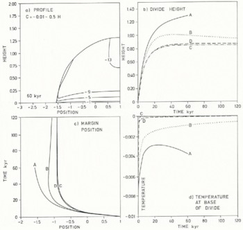
Fig. 11. Illustrating warm-bottomed divides with cases (a) C(Z) = −0.01 − 0.50Z; (b) C(Z) = −0.01 −0.25Z; (c) C(Z) = −0.01 − 0.25Z, model 2 latent-heat representation; and (d) C(Z) = −0.01 − 0.50Z, high geothermal heat case; Figure 11(a) case A after 60 ka; Figure 11(b) divide heights against time; Figure 11(c) margin position against time; Figure 11(d) temperature at the base of the divide against time. Note the similarity between cases (c) and (d), and how (a) adopts a cooling mode after 20 ka.
The ice sheets displayed no evidence of a propensity to collapse as a result of having a warm-based divide, because the warming of the divide is driven by conduction, the slowest acting of all the processes. This means that the ice sheet has more than enough time always to adjust kinematically to the new temperature distribution.
Since the warming was conduction-driven, we investigated the effects of changing the thermal inertia by (i) setting L = −0.25 but changing the pseudo-latent heat representation to model 2 (Fig. 3, graph B) (case C); and (ii) setting L = −0.5 and increasing the geothermal heat gradient by a factor of 20 (case D). The results of these calculations are nearly the same (Fig. 11); this is quite remarkable in view of the differences between cases A and B. The reason appears to be the nearly identical heating histories of the divide base, which arises from the low thermal inertias of the system. The ice sheet is prevented from becoming over-thickened because the warm base of the divide permits greater deformation, and shows monotone relaxation into steady state.
We have also carried out calculations with an undulating topography and ones with isostatic deflection included. These made no difference to the modes of operation of the system as described above. Calculations which included a temperature-field warming as X decreased also had no effect upon the mode of operation, though in this context we mention that it is extremely difficult to cause an ice sheet to advance over a soft bed.
7. Discussion
We summarize the results:
-
(i) The temperature field just in from the margin is dissipation-driven. The heat production in most cases is sufficient to bring the zone just inside the margin to the melting point. Conduction is more efficient over these small thicknesses and advection of cold into the area is not important.
-
(ii) The temperature field at the base of the divide area can adopt two modes. One is a cold-based mode, where the ice sheet is thicker and the low temperatures are due to the advection in cold ice from altitude. The other mode is warm-based and is associated with thin ice sheets and warm conditions. This is not a bifurcation in the strict sense (cf. Reference Veen van der and Oerlemansvan der Veen and Oerlemans, 1984), but there is a sensitive range of parameter values which stimulates a bifurcation.
We have not demonstrated a multiple steady-state solution and, if there were one, then the fastest agent of heat transfer to produce a change from cold-based to warm-based is conduction, which operates upon a far slower time-scale than the kinematical processes of adjustment at the divide, meaning that a collapse is extremely unlikely (cf. the initiation waves of Fowler (1987) which operate on time-scales of hours and days to start valley-glacier surges).
Ice sheets will grow until they have sufficient area in the ablation zone to balance the accumulation zone. The much higher velocities and the fact that ablation is an order of magnitude greater than accumulation means the areal extent of the accumulation is usually an order of magnitude greater than the ablation zone (see e.g. Fig. 2). The total ablation is, in consequence, quite sensitively dependent upon the geometry of the marginal areas, and this effect is amplified by the fact that ablation is greatest at the very margin.
The equilibrium margin slope is dependent upon bed roughness and marginal ablation (e.g. Hutter, 1983; Morland and Smith, 1984), while the margin-slope evolution is dependent upon spatial derivatives of these quantities. In our model, the marginal temperature is defined by a Dirichlet condition. In cases where the bed roughness is temperature-dependent, this therefore defines the marginal roughness (see the great variation caused by temperature on margin slope in Figure 9, for example).
There is a very large amount of evidence which indicates that processes of basal motion in marginal areas are rather different from those in core areas. We believe that the principal difference is the existence of large amounts of debris underneath the ice sheet (Reference Boulton and HindmarshBoulton and Hindmarsh, 1987) which can deform. There is evidence from many areas (Reference BoultonBoulton, 1987) that this was a significant process underneath at least the marginal areas of the Quaternary mid-latitude ice sheets. There is also evidence of foreland pushing by these ice sheets. We believe that this could only have occurred when the sediment was unfrozen; furthermore, the fact of foreland pushing implies that the stress distribution in the coupled ice-sheet/substrate system is not simply that of the shear-stress gradient balancing the pressure gradient; stresses are also being transmitted longitudinally.
The transmission of these stresses and the consequent strain-rates are dependent on the temperature of the foreland and in particular whether it is frozen or unfrozen. Geological evidence suggests that the foreland areas were permafrost areas. Exactly what this implies about the temperature of the ice at the margin is not clear as, according to our model, warm ice would be advected from the zones of high dissipation. (The fact that the ice cools down in our model is really a consequence of applying a forced boundary condition to a hyperbolic outlet.) The exact distribution of marginal temperature then becomes a very complex problem. Furthermore, the mid-latitude ice sheets were often flanked by very large pro-glacial lakes. These would have insulated the margins from the annual temperature variations and kept the area at the melting point.
The thrust of these arguments is that the processes of enhanced basal deformation at the margin is dependent, perhaps quite significantly in view of the differing strengths of frozen and unfrozen sediments, upon details of the margin stress and temperature fields. The governing equations for ice-sheet-profile evolution (Equation (13)) at the margin incorporate no diffusion, and are in principle sensitive to very small perturbations. The kinematical sensitivity of the margin is capable of amplifying these perturbations. It is likely that a more sophisticated model of margin mechanics would include diffusive or dispersive terms (as in Hutter, 1981) which might damp out sensitivity. We suggest that a more detailed model of the margin, including coupling with the bed, is necessary.
Fowler’s (1980) conjecture that only the base of an ice sheet will ever reach the melting point seems to be correct when vertical velocities are directed downwards. The bulging associated with compression will, however, advect warm ice upwards, meaning that the margins may become temperate. There is ample evidence to suggest that ice sheets do compress at the margin (Reference BoultonBoulton, 1987). This means that some kind of representation of temperate ice will be necessary in an ice-sheet model (see also the computations of Hutter and others (1986)). In dissipation-driven areas, it does not seem that the details of our enthalpy formulation of the model are important, but are rather more so in the divide area.
Comparison of our results of basal temperature with those of Oerlemans and van der Veen (1984, fig. 5.8) show that our computed warm patches lie somewhat closer to the margin than do those of Oerlemans and van der Veen. It is simple to explain this observation in terms of the different basal sliding laws used. In the cases where the basal slip is not temperature-dependent, using the Morland and others sliding law (relation (8)) predicts basal power generation (relation (17)) to vary as H(∂H/∂X)2, while Oerlemans and van der Veen, who use a Weertman functional form (relation (22)), have the basal power generation varying as (H∂H/∂X)m, where m ≥ 2. The geometry of ice sheets dictates that the Oerlemans and van der Veen position of maximum basal power generation must lie further in than ours. Since the margin is kinematically very sensitive, this implies that not only the magnitudes of the coefficients inserted into sliding laws are important but also the functional form, since if a Weertman form implies cold margins we should expect steeper ice-sheet surface gradients and larger ice sheets.
A further inference that may be made from the basal temperature profiles is that regional refreezing is likely to be limited to a marginal zone. These show that a moving basal particle of ice is warmed nearly as far as the margin. It is only when heat is being removed from the ice that it can use the latent heat available in water. This is not a statement that regelation will not occur but that zones of refreezing should be limited. This statement must be qualified in a number of ways. First, in our model we have taken no account of the fact that the rheology of ice is implicitly pressure-dependent, as the correct temperature to chose (Reference RigsbyRigsby, 1958) in the constitutive relation is the homologous temperature. Wet ice being moved into a region of lower pressure at a constant absolute temperature is having its homologous temperature lowered, and will therefore become stiffer, and susceptible to refreezing. Owing to the dissipation-dominated thermal behaviour near the margin, we doubt that the ice could cool down, but it may be that depressurizing in areas of thick ice from ice being forced upwards by topography could occur faster than heating by conduction, and refreezing would occur here. This may be the case at Byrd Station. However, if the marginal zone of refreezing is larger than our model suggests, the implication is that the marginal model needs improvement. We doubt that adopting a Weertman sliding law is sufficient.
The difference in profiles obtained by the prescribed temperature fields of Reference Morland, Smith and BoultonMorland and Smith (1984) and of Hutter and others (1986) may be explained in terms of the self-regulatory structures of ice-sheet temperature profiles. Morland and Smith produced very flat profiles when they had cold margins and warm divides. As we have shown, this temperature structure does not appear to be admissible because of the nature of the processes which determine the structure of temperature fields within ice sheets.
These results have several implications for geological interpretations:
-
(i) The sensitivity of the marginal area increases the importance of the evidence from this area. The tectonic deformation of soft sediments beneath the ice sheet and the structures thereby formed contain information which is amplified by the kinematics of the margin to have implications on the scale of the ice sheet itself.
-
(ii) Zones of refreezing are predicted to be limited except when topographic effects occur. If refreezing is important, this contains information about the functional form of the ice-sheet profile. The areal extent of warm ice, interpretable by geological evidence, is dependent quite sensitively upon the lapse rate, which may therefore be constrained by geological evidence.
Finally, we have an alternative position on whether there is a shear-heating instability in ice sheets (see, for example, Reference Clarke, Nitsan and PatersonClarke and others, 1977; Reference FowlerFowler, 1980; Reference Yuen, Saari and SchubertYuen and others, 1986). Since the marginal areas reach the melting point, there is always an approach to high temperature fueled by dissipation, i.e. the phenomenology of a shear-heating instability. However, because these high temperatures are attained very early, they are part of the ice sheet. We have shown that ice sheets can, nonetheless, grow with very warm margins. The divide areas produce very low shear heat and we have shown that kinematical adjustment is at least as fast as any warming process. Thus, the thermal phenomenology of a shear-heating instability will usually (always?) exist, but this ever-presence implies no spectacular kinematical consequences.
8. Conclusions
-
(i) Continental ice-sheet temperature fields evolve according to processes occurring at three time-scales: a dissipative time-scale of the order of thousands of years, an advective time-scale of the order of tens of thousands of years, and a conductive time-scale of the order of 100 000 years. Dissipation is the most important process in the marginal areas, advection in the upper regions of the divide area, and conduction in the basal divide area.
-
(ii) Ice-sheet kinematics have two time-scales: an advective one of thousands of years and a diffusive one of tens of thousands of years. They are most dominant in the marginal and central areas, respectively.
-
(iii) Dissipation drives marginal temperatures up to the melting point very rapidly; however, the form of the sliding law we use probably exaggerates this effect.
-
(iv) Temperatures at the base of the divide are able to adopt two modes: a cooling one, associated with thickening of the ice sheet and a warming mode associated with low ice sheets. The latter is produced by low lapse rates and low thermal inertia, but we have not conducted a full search of the possible parameter variations. We do not believe that the warming mode leads to an instability, as the warming is due to conduction which operates on a very much slower time-scale than does mechanical adjustment.
-
(v) The marginal area shows extreme kinematical sensitivity and, with the model we use, acts to amplify the effects of the marginal mechanics. This fact is also true of other one-dimensional models. Longitudinal gradients are not negligible at the margin, and this problem is made more acute by the existence of deformable materials underneath these areas of ice sheets. The thermal regime at the marginal area could be of extreme importance, and blanketing by pro-glacial lakes could even be of importance in determining marginal motion. The kinematical sensitivity of the margin increases the importance of the deforming-bed problem.
-
(vi) The small-aspect ratio of the bed-temperature interference problem means that horizontal conduction of heat is not likely to occur except in marginal areas. The thermal inertia of the bed is important and may alter the geothermal heat gradient significantly. We do not believe that this will alter the modes of operation of ice sheets, because conduction is the slowest process operating and the ice sheet can therefore adjust to these changes.
-
(vii) Continental ice sheets may have had temperate margins.
-
(viii) The shear-heated approach to melting of the margins always seems to be present and seems to rule out the possibility of a shear-heated collapse of large ice sheets.
-
(ix) The study has highlighted the inadequacies of numerical and mechanical models of the marginal areas. A more refined model of the mechanics and the coupled bed/ice-sheet thermal problem is needed and will dictate the numerical strategy needed.
Acknowledgements
This work was carried out as part of U.K. Natural Environment Research Council grant GR3/6737, “The temporal and spatial dynamics in relation to their geological products”. We had useful conversations with A. Fowler about approximate representations of the effects of phase transitions and with L. Morland about the reduced model.


