ANTARCTIC ICEBERG OBSERVATIONS: TECHNIQUES AND RESULTS

Available information on the distribution of small and medium-sized icebergs in the Southern Ocean comes primarily from two major sources: satellite-data-based estimates and in situ ship-based observations. Both approaches and corresponding datasets have their own advantages and weaknesses.

The high spatial resolution and all-weather capability of satellite-based SAR make these observations attractive for monitoring Antarctic icebergs. Examples of applications of SAR data to estimate the iceberg concentration and iceberg drift patterns over the Weddell Sea and over the Indian Ocean Sector of Antarctica have been presented correspondingly by Gladstone and Bigg (Reference Gladstone and Bigg2002) and Young and others (Reference Young, Turner, Hyland and Williams1998). Wesche and Dierking (Reference Wesche and Dierking2015) identified icebergs in the SAR-based mosaic over Antarctica and found considerable regional variations in the iceberg size distribution. Speckles affecting SAR imagery present a serious issue complicating both automated and manual identification of small icebergs with a size of less than several SAR pixels (or below ~100 m). Until the recently rare availability of the imagery over the Southern Ocean and its high-cost limited iceberg monitoring with SAR data. This situation is expected to improve with the recent launch of Sentinel-1 satellites providing free high spatial resolution radar imagery to the public.

Satellite altimeter data present another source of information on Antarctic icebergs. Retrieval technique and first results of iceberg identification with altimeter data are presented by Tournadre and others (Reference Tournadre, Whitmer and Girard-Ardhuin2008, Reference Tournadre, Girard-Arghuin and Legresy2012). A more comprehensive processing of altimeter observations since 1994 resulted in an extensive iceberg dataset and a corresponding spatially-detailed map of iceberg concentration in the Southern Ocean (Tournadre and others, Reference Tournadre, Bouhier, Girard-Ardhuin and Remy2016). Similar to SAR, radar altimeter observations are weather independent; however, iceberg identification with altimeter data requires ice-free water conditions and relies on the assumed iceberg freeboard elevation and reflectivity. Furthermore, due to specifics of radar altimeter data retrievals are limited to icebergs with a height of <15 m and with a size between 0.3 and 8.0 km².

Ship observations, providing information on the concentration and the size of icebergs, have been used to characterize the Antarctic iceberg distribution since the early 1960s. Nazarov (Reference Nazarov1962) compiled a map summarizing Antarctic iceberg sightings since the late 18th century to the middle of the 20th century. According to this chart, icebergs were seen as far north as 40° S in the Atlantic and Indian sectors and up to 50° S in the Pacific sector of the Southern Ocean. One of the first charts of iceberg drift in Antarctica was presented by Shilnikov (Reference Shilnikov and Tolstikov1969). Buinitskii (Reference Buinitskii1973) produced a map of the mean iceberg concentration in the Indian Ocean sector of the Southern Ocean. Burrows (Reference Burrows1976) compiled information on the largest distance from the coast of Antarctica where icebergs were sighted. According to his study icebergs can travel as far north as 30°–34° S within 90° W to 90° E longitudes and up to 40°–42° S within 90° E–90° W. Later studies however never confirmed iceberg sightings at such low latitudes (e.g., Orheim, Reference Orheim1990). Gradual accumulation of in situ iceberg observation data in the last three decades has allowed for a progressively more detailed characterization of the spatial distribution of Antarctic icebergs in various regions of the Southern Ocean (Wadhams and others, Reference Wadhams1988; Koshlyakov and others, Reference Koshlyakov, Belkin, Radikevich and Romanov1993; Romanov, Reference Romanov, Popov and Voevodin1996a, Reference Romanovb; Jacka and Giles, Reference Jacka and Giles2007; Romanov and others, Reference Romanov, Romanova and Romanov2008; Orheim, Reference Orheim2015) as well as their seasonal changes (e.g., Romanov and Korotkov, Reference Romanov and Korotkov2001; Romanov and Romanova, Reference Romanov and Romanova2003, Reference Romanov and Romanova2005).

There is a substantial interest in estimating area-integrated characteristics of icebergs, particularly their number, surface area and volume. This information presents an important input to studies and estimates of the iceberg calving rates, freshwater flux provided by icebergs, global sea-level change, mass balance of the Antarctic ice sheet and the iceberg impact on the Antarctic ecosystem dynamics. Silva and others (Reference Silva, Bigg and Nicholls2006) used satellite-based information on the size of giant icebergs calving off Antarctic ice shelves and found that the mass of these icebergs can reach ~6000 Gt a⁻¹. The annual mass of calving icebergs averaged over the time period from 1979 to 2003 however was noticeably smaller and amounted to 1089 ± 300 Gt. Given an assumed ice density of 850 kg m⁻³ (Jacobs and others, Reference Jacobs, Helmer, Doake, Jenkins and Frolich1992) this equates to a freshwater volume of 1281 ± 353 km³. Considerably larger estimates of the total iceberg volume, of 22 000 km³ in 2002 and 9000 km³ in 2012, are given by Tournadre and others (Reference Tournadre, Bouhier, Girard-Ardhuin and Remi2015), who used NIC and Brigham Young University data on large icebergs. Wesche and Dierking (Reference Wesche and Dierking2015) placed the estimated instantaneous mass of Antarctic icebergs to within 5167–7440 Gt (or 6079–8753 km³); however, this estimate included only icebergs in the near coastal zone. Tournadre and others (Reference Tournadre, Girard-Arghuin and Legresy2012) examined smaller icebergs with a size of 100–2800 m in the area north of 66° S and estimated their weight equal to 400 Gt. Expanding the analysis to Antarctic coastal waters these authors obtained an estimated total weight of icebergs of ~600 Gt, which is equivalent to the volume of 706 km³ (Tournadre and others, Reference Tournadre, Bouhier, Girard-Ardhuin and Remy2016).

Similar to the satellite-based remote-sensing retrievals, estimates of the total mass and volume of Antarctic icebergs derived from ship observations also vary substantially. The range of reported estimates of the total volume of icebergs simultaneously floating or grounded in the Southern Ocean (or instantaneous iceberg volume) spans from 4700 km³ (Romanov, Reference Romanov, Popov and Voevodin1996a) to 17 900 km³ (Shilnikov, Reference Shilnikov1960). Other estimates of the total iceberg volume amounting to 5600, 8200, 12 000 and 12 500 km³ have been provided correspondingly by Buinitskii (Reference Buinitskii1973), Schell (Reference Schell1974), Losev (Reference Losev1982) and Orheim (Reference Orheim1985).

A wide spread in the estimated values of the iceberg volume is due to high spatio-temporal variations of the Antarctic icebergs distribution and to a relatively small number of available iceberg observations. Most estimates of the total iceberg count and iceberg volume in Antarctica have been made using observations over a limited area and extrapolating the results to the entire Southern Ocean (e.g., Buinitskii (Reference Buinitskii1973), Shilnikov (Reference Shilnikov1960), Losev (Reference Losev1982)). Another reason for the large scatter in the estimated total volume of icebergs is uncertainty with respect to geometrical characteristics of icebergs, particularly to their size and shape. Assumptions on the iceberg geometrical properties, particularly on the relationship between the iceberg length, width and height and on their shape varied from one study to another and often were based on very limited statistics. Generating more accurate and more physically justified estimates of the iceberg volume and mass requires utilizing more spatially extensive and detailed information on the iceberg concentration and improved statistics of the iceberg morphometric properties.

IN SITU ICEBERG OBSERVATIONS DATASET

The Antarctic iceberg dataset collected and maintained jointly by Shirshov Institute of Oceanology of the Russian Academy of Sciences and AARI incorporates information obtained through iceberg observations from ships traveling in the Southern Ocean. The dataset is routinely updated with recent observations and newly recovered historical data. The core of the dataset comprises ~45 000 iceberg observation reports delivered since the middle of the 1950s from the research vessels of AARI. These data were rescued and recovered from the original ship ice and weather log journals archived at AARI. Most reports provide only the number count of icebergs sighted by the observer. The dataset also incorporates the results of ~4000 ship observations of icebergs performed according to the guidelines of the Norwegian Polar Institute, NPI (Orheim, Reference Orheim1980) over the period from 1978 to 1987. Within this program observers were requested to report the iceberg amount within five size range categories, 10–50, 50–200, 200–500, 500–1000 and 1000 m. The results of ~7000 observations conducted under the auspices of the Australian Antarctic Program (AAP) during the period from 1978 to 2001, were acquired from the dataset compiled by Dr T. Jacka (https://data.aad.gov.au/metadata/records/climate_iceberg). Similarly to NPI, AAP iceberg reports included both the total number of icebergs and the iceberg quantity in a number of size categories. The AAP size categories however were different from those of NPI and covered a wider range from 25 to 3200 m. Finally, over 4000 iceberg records made in Antarctica from Russian whaling ships in 1947–59 were recovered from various reports on these cruises. The majority of observations incorporated in the dataset (~90%) were performed during the warm season from December to April (see Table 1).

Table 1.

Distribution of observation records of the iceberg concentration by the month of the year

In about three-quarters of observation records comprising the dataset, icebergs have been identified and counted using the ship radar. The remainder of reports, mostly dating back to the 1940s–1960s, are based on visual observations. In the reports, information on the iceberg concentration is provided as the number count of icebergs within a circle of a certain radius. Both the size of the circle and the time interval between consecutive observations may vary. At AARI the radius of the circle is set to 15 nm (27.8 km), whereas observations are typically performed every 1.5–3 h. The time interval varies depending on the ship speed to avoid overlapping of the observing circles and double-counting of the icebergs. When examining and processing the data we did not specifically check for possible multiple recording of the same icebergs by two or more ships traveling in the same region at the same time since these instances are very rare.

The NPI guidelines instruct to report the number of icebergs within a circle of 12 nm radius and to perform observations every 6 h. Within the AAP iceberg counts were performed every 3 h within a smaller, 6 nm range. In both latter cases, the ship velocity of 4 knots or higher ensures no overlap of consecutive observations. Within all three major iceberg observation programs (NPI, AAP and AARI) observers report cases when no icebergs were seen. These observations are recorded as ‘no iceberg sightings’, to distinguish between cases where there were no icebergs and where no observations were made.

Routine iceberg observation and reporting typically starts with the sighting of the first iceberg on the ship route and ends when on several consecutive observation times no icebergs were observed. The lack of explicit ‘zero’ iceberg number reporting immediately north of the location of the first and of the last iceberg sighted presents a considerable problem since it causes an overestimate of the mean concentration in the area of intermittent iceberg occurrence. To ensure adequate characterization of the iceberg distribution across the Antarctic region, in this study the AARI iceberg records were complemented with synthesized ‘no iceberg sighting’ reports. These reports were generated for the time and location of each meteorological observation taken at 3 h time interval along the ship route south of 46° S preceding the first and following the last iceberg sighting.

When processing the iceberg observation data we consider iceberg counts obtained from visual and from radar observations comparable. This approach is justified by the results of Dowdeswell and others (Reference Dowdeswell, Whittington and Hodgkins1992) who reported only a small, within 5%, the difference between the iceberg amounts estimated visually and with the radar-based technique. Reported iceberg quantities are also corrected to account for a gradually decreasing success rate of radar-based iceberg detection with distance from the radar. Following Wadhams (Reference Wadhams1988) we assume a linear decrease of the detection success rate from 100% at 8 nm to 0% at 22 nm. To achieve consistency between observations made over different areas we adopted the 15 nm range as a standard and adjusted all reported iceberg quantities to this range. For convenience in this paper, the iceberg quantity within the standard 15 nm distance range is further referred to as the iceberg concentration. Simple geometrical considerations allow for converting this value to the number of icebergs within a certain area, e.g., the iceberg concentration of 100 corresponds to approximately four icebergs per 10 km × 10 km square box.

Aside from the iceberg number counts more detailed iceberg observations that specifically focused on the iceberg shape characterization were conducted during several cruises of r/v ‘Professor Wiese’ in 1973–90. During these cruises the iceberg concentration observations were complemented with counts of the number of icebergs of different shapes. The reports included both the overall amount of iceberg sighted and the number count of icebergs of each of five basic shapes, tabular, dome-shaped, sloping, pinnacle and weathered. The dataset includes 1777 such ‘iceberg number count by shape’ observations incorporating information on more than 21 000 individual icebergs.

In a number of AARI cruises, observations of the iceberg concentration were accompanied by measurements of the morphometric characteristics of selected individual icebergs. The iceberg shape was determined visually whereas the iceberg length and freeboard elevation were measured with a sextant and a rangefinder. Our dataset contains information on geometrical parameters of 4130 icebergs of different shapes collected since 1957. Table 2 presents the distribution of the number of iceberg observations of the two latter types (iceberg number count by shape and iceberg geometry by shape) by the month of the year. Similar to the iceberg concentration, most these observations were performed during the warm season of the year.

Table 2.

Number of available detailed observations of iceberg shape and size by the month of the year

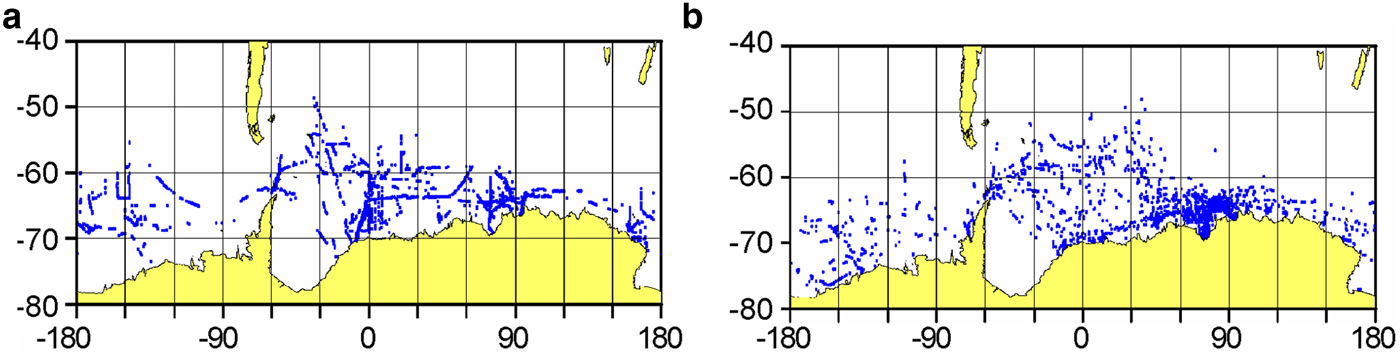
Figure 1 shows the geographic distribution of collected iceberg number count records including synthesized zero iceberg concentration reports. This distribution is highly uneven: no records are available in the south-west of the Weddell Sea, in the southeast of the Pacific sector and in a number of coastal regions of the Indian Ocean sector of the Southern Ocean. At the same time, there is a large density in the coastal area within 60° E to 120° E next to the location of most Russian and Australian Antarctic stations and within 60° W to 50° E longitude away from the coast. These areas are most frequently traveled through by Antarctic supply ships. Similar to the iceberg concentration measurements, most detailed observations of the iceberg shapes and geometrical characteristics have been conducted in the Atlantic sector of the Southern Ocean (see Fig. 2).

Fig. 1.

Location of ship observations of the iceberg concentration in the Southern Ocean performed during the time period from 1958 to 2014. Eastern longitudes are positive and western longitudes are negative.

Fig. 2.

Location of detailed observations of iceberg properties. (a) Observations of number count by shape made from the r/v ‘Professor Wiese’ in 1980–1988. (b) Observations of iceberg geometry by shape made in 1957–2014. Eastern longitudes are positive and western longitudes are negative.

ICEBERG CONCENTRATION AND GEOGRAPHICAL DISTRIBUTION

Figure 3a presents a map of the mean iceberg concentration in the Southern Ocean derived from the iceberg concentration reports contained in the collected dataset. The map was generated by aggregating all available iceberg observation records within 1° latitude and 2° longitude grid cells, bringing the reported iceberg number count to the standard 15 nm range and averaging this number within each grid cell. As such the map is meant to represent the average (or the most typical instantaneous) distribution of the iceberg concentration in the Southern Ocean over the 60+ years period covered by the dataset.

Fig. 3.

(a) Map of the mean iceberg concentration in grid cells of 1° latitude by 2° longitude. Iceberg concentration is expressed as the number of icebergs sighted within 15 nm range from the ship). Grid cells with no observations are left blank. The blue line shows the location of the polar ocean front; the black line shows the southern boundary of the ACC according to Orsi and Ryan (Reference Orsi and Ryan2001). (b) Mean atmospheric pressure at sea level (hPa) from October to March over the 60-year period from 1950 to 2010 calculated using monthly mean sea surface pressure data of Hadley Centre (http://hadobs.metoffice.com/hadslp2/data).

The map in Fig. 3a distinctly shows three known clusters of elevated iceberg concentration in Antarctica located in the Atlantic Ocean within 0°–60° W, in the Indian Ocean within 40°–120° E and in the Southern Pacific within 90°–170° W (e.g., Schodlok and others, Reference Schodlok, Hellmer, Rohardt and Fahrbach2006, Jacka and Giles, Reference Jacka and Giles2007, Romanov and others, Reference Romanov, Romanova and Romanov2008, Orheim, Reference Orheim2015, Tournadre and others, Reference Tournadre, Bouhier, Girard-Ardhuin and Remy2016). The area in the Atlantic Ocean corresponding to the Weddell Sea has the maximum northward extension with large numbers of icebergs north of 50° S. At the same time the largest iceberg concentrations, often exceeding 30 icebergs within a 15 nm range, occur in the other two areas in the Indian and Pacific Sectors of the Southern Ocean.

In the coastal zone, the iceberg concentration depends on the productivity of nearby glaciers, their structure (Rignot and others, Reference Rignot, Jackobs, Mouginot and Scheuchl2013; Wesche and others, Reference Wesche, Jansen and Dierking2013), the prevailing ocean currents and peculiarities of the bottom topography. In particular smaller iceberg concentrations are observed at 20°–35° E next to the Princess Ragnhild Coast where there are no productive glaciers (Williams and Ferrigno, Reference Williams and Ferrigno1988; Rignot and others, Reference Rignot, Jackobs, Mouginot and Scheuchl2013). Iceberg drifting to this region with the coastal eastward-ward current is hampered by a sharp cape at ~34° E and the area of shallow waters extending northwards of this cape. Larger iceberg concentrations are seen at the location of Amery (~70° E–75° E), Shackleton (~95° E–100° E), West (80° E–90° E) and Getz (~120° W–140° W) ice shelves.

Away from the shore the spatial distribution of the iceberg concentration is determined to a large extent by peculiarities of the atmospheric circulation. In summer, from October to March, three stable cyclonic pressure systems develop in the Southern Ocean with centers at ~120° W, 30° E and 110° E (see Fig. 3b). Southerly winds at the western periphery of these pressure systems transfer a large number of icebergs to the north into the open ocean and thus cause the increase of their concentration. Northerly winds at the eastern periphery of atmospheric cyclones cause icebergs to drift closer to the coast creating large areas of small iceberg concentrations in the open ocean to the east, and sometimes in the center of these cyclones. The stability of the pattern of the atmospheric circulation throughout the year ensures the stability of this iceberg distribution pattern.

An interesting feature in the iceberg distribution is their relatively small concentration in the Ross Sea region (160° E to 150° W) both along the coast and further out in the open ocean, which may seem inconsistent with the presence of the large Ross Ice Shelf. A feasible physical explanation of small concentrations of icebergs in the Ross Sea is that southerly winds prevailing in this region (Nigro and Cossano, Reference Nigro and Cossano2014) may be sufficiently stable and strong to ensure a rapid removal of icebergs along with the sea ice away from the coast. An overall small number of icebergs may also be due to the fact that the Ross Ice Shelf tends to generate predominantly large icebergs. Support for this latter hypothesis is provided in particular by Wesche and others (Reference Wesche, Jansen and Dierking2013) who observed a specific structure of cracks in the Ross Ice Shelf.

The eastern periphery of one of the low-pressure regions in Antarctica is steadily located over the west of the Weddell Sea, west of 40°–50° W (see Fig. 3). Therefore winds of northerly directions should dominate here throughout the whole year. These winds are generally expected to prevent the removal of icebergs from this region to the north and northeast. The fact that a large number of icebergs is observed in the northwestern Weddell Sea, west of 30° W, indicates that iceberg drift patterns in the Weddell Sea are mostly determined by ocean currents.

As seen in Fig. 3, the northern boundary of the iceberg occurrence (NBIO) essentially coincides with the position of the oceanic Polar Front (PF). This can be explained by a so-called zone of oceanic convergence associated with the PF, where southerly and northerly flows at the ocean surface converge and thus prevent icebergs from drifting into lower latitudes. The PF is also associated with a large temperature contrast of sea-surface waters. When examining temperatures in the 0–200 m top ocean layer in the Drake Passage, Sprintall and others (Reference Sprintall, Chereskin and Sweency2012) found a substantial temperature change from 3 to 5 °C north of the PF down to −1 °C immediately to the south. It is obvious that icebergs would be more sustainable in colder waters south of the PF than in warmer waters north of it.

In some areas, however, the NBIO clearly deviates from the PF. This happens in particular, at 50°–80° E where it is located considerably south of the PF. We attribute this to the fact that at these longitudes there is no iceberg removal from coastal areas to the north whereas icebergs carried out of the Weddell Sea and drifting eastward along with the Antarctic Circumpolar Current (ACC) decay before reaching these longitudes. An opposite situation is seen at 0°–30° E longitude where NBIO extends northwards past the PF and reaches 44°–46° S parallel. Penetration of icebergs to such low latitudes may be facilitated by frequent oceanic eddies that develop at the borders of the ACC and Agulhas current (e.g., Dencausse and others, Reference Dencausse, Arhan and Speich1989). Another region where Antarctic icebergs are frequently seen beyond the PF is located at ~100°–120° E. The band of larger iceberg concentration extending north-east past 50° S and crossing the PF in this region is created by a strong northward ocean current component at ~85° E, east of Kerguelen Plateau (McCartney and Donohue, Reference McCartney and Donohue2007). It causes icebergs to escape from the coastal current and drift northward. Some of these icebergs occasionally reach the coast of New Zealand (Burrow, Reference Burrow2005).

Although the number of available iceberg reports is relatively large, they are distributed across the Antarctic region unevenly leaving some areas of Antarctica with no records at all. As seen in Fig. 4a, the coverage of the Atlantic and Indian sector of the Southern Ocean with iceberg observation data is clearly better than the coverage of the Pacific sector. Variability of the iceberg occurrence (Fig. 4b) exhibits a spatial pattern similar to the one seen in the distribution of the mean values. The RMS deviation of the iceberg concentration averaged over all ocean grid cells covered with observations amounted to 8.0, which is almost equal to the grid cell mean value of the iceberg concentration of 8.4. Further analysis of the iceberg observation statistics shows that cases with no icebergs in sight occur quite often. Non-zero minimum iceberg concentration is found only in ~15% of all grid cells. Figure 4c shows that in the Eastern Hemisphere these grid cells are located mostly within a narrow coastal zone whereas in the Western Hemisphere such locations are found both in the coastal area and in the open ocean. The spatial distribution of the maximum iceberg concentration (Fig. 4d), iceberg-free occurrence (Fig. 4e) and the frequency of occurrence of iceberg concentration of over 10 icebergs per circle of 15 nm radius (Fig. 4f) generally follows the spatial distribution of the mean iceberg concentration. The maximum iceberg concentration along with the smallest values of the iceberg-free occurrence corresponds to the Weddell Sea and the area north of it within 0°–60° W, the coastal zone next to Amery, West and Shackleton glaciers, within 60°–120° E, and to the Ross and Amundsen Sea region within 120°–160° W.

Fig. 4.

Iceberg statistics. (a) The number of iceberg number count reports in grid cells of 1° latitude by 2° longitude. (b) Standard deviation of the observed iceberg concentration. (c) Minimum observed iceberg concentration. (d) Maximum observed iceberg concentration. (e) Frequency of occurrence of iceberg-free waters (in percent). (f) Frequency of occurrence of the iceberg concentration exceeding ten icebergs within the circle of 15 nm radius (in percent) Iceberg concentration is expressed as the number of within a circle of 15 nm radius.

The amount of available iceberg observations presents a factor affecting the derived statistics of the iceberg concentration. This concerns primarily the minimum and maximum values of the iceberg concentration, which tends correspondingly to decrease and increase with increasing size of the sample. Therefore estimates of extreme values of the iceberg concentration made for grid cells with few observations may not be reliable and should be used with care. This applies in particular to the Pacific sector of the Southern Ocean and to the central part of the Weddell Sea where most grid cells are covered with fewer than ten reports of the iceberg concentration. Estimates of the mean iceberg concentration may also be affected by the limited number of observations. As was shown earlier there is good correspondence between the derived iceberg concentration and major physical factors controlling the iceberg distribution (i.e. glacier productivity, wind and ocean current patterns). This may be considered as evidence that despite a small number of observations in some areas the derived map of the iceberg concentration realistically characterizes the iceberg distribution in Antarctica.

TOTAL ICEBERG COUNT

An estimate of the total instantaneous number of icebergs in Antarctica has been obtained through integration of the derived spatial distribution of the iceberg concentration over the surface of the Southern Ocean. Discontinuities in the iceberg concentration map caused by unavailability of iceberg observations were eliminated with two different techniques. A simple bilinear interpolation has been applied to fill in gaps in the area coverage of the available iceberg concentration map in the open ocean. In the coastal areas, characterized by potentially large spatial gradients of the iceberg concentration, we have used a more sophisticated approach, which accounts for the proximity of iceberg-generating glaciers and their productivity.

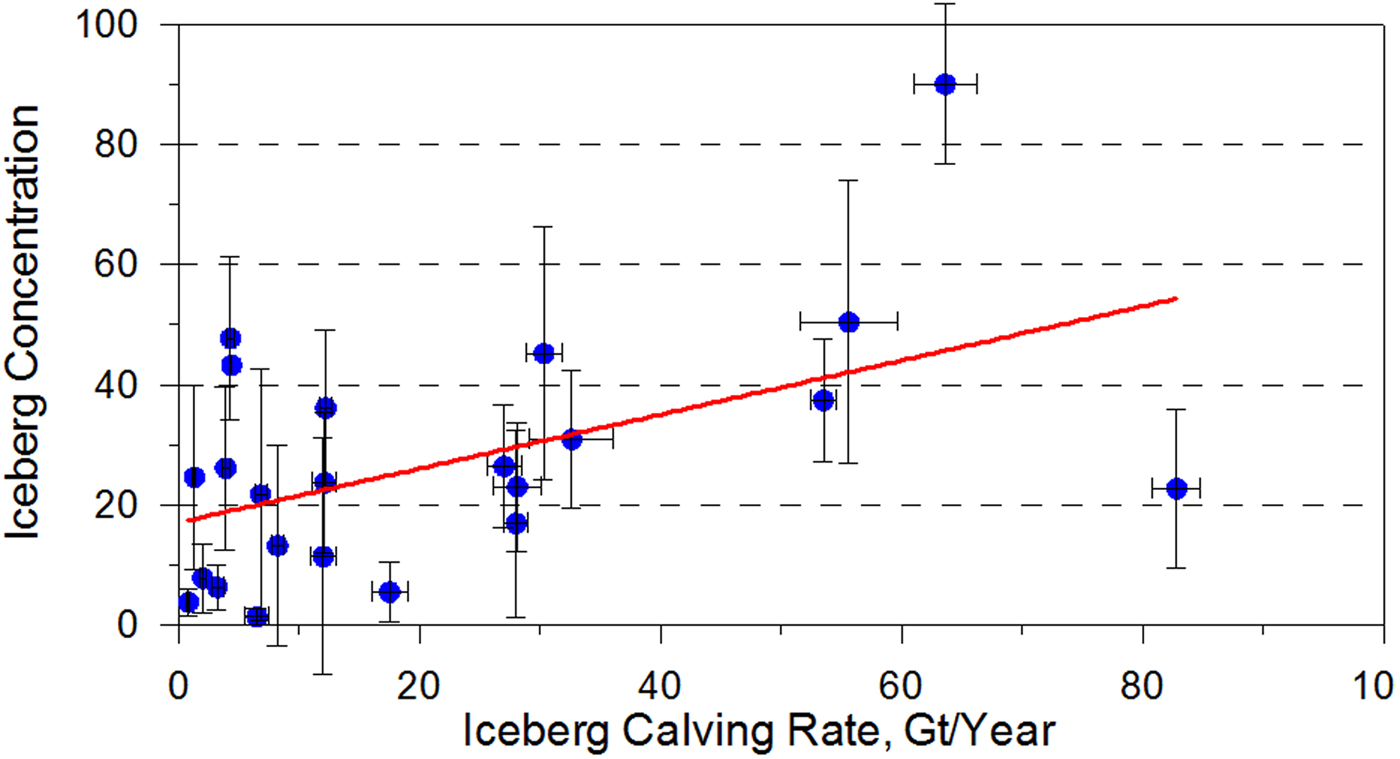
In this latter approach, the relationship between the glacier characteristics and the iceberg concentration in adjacent coastal zones was established using estimates by Rignot and others (Reference Rignot, Jackobs, Mouginot and Scheuchl2013) of the Antarctic glaciers ice front flux, which is the proxy for the calving flux or glacier productivity. These data were matched with the mean iceberg concentration calculated for grid cells of 2° latitude by 5° longitude adjacent to the glacier location. Only grid cells with over 30 iceberg observation records were used. From more than 60 glaciers surveyed by Rignot and others (Reference Rignot, Jackobs, Mouginot and Scheuchl2013) sufficient matching iceberg concentration data were found for 23 glaciers. A certain weakness of this approach consists in the fact that information on the glacier productivity rates and iceberg concentration does not quite match in time: Rignot and others (Reference Rignot, Jackobs, Mouginot and Scheuchl2013) estimates generally represent the calving flux in the first decade of the 21st century whereas collected iceberg concentration data refer to the last 60+ years time period. Still the correlation statistics presented in Table 3 and a corresponding plot in Fig. 5 demonstrate a well-pronounced positive correlation between the iceberg concentration and the glacier productivity (R = 0.49, R ² = 0.26, statistically significant at the 0.01 level). The relationship between the two parameters was approximated with a linear function (Y = 0.45X + 17.00) and was further applied to estimate the iceberg concentration in the coastal grid cells adjacent to glaciers where in situ iceberg observations were lacking.

Fig. 5.

The relationship between the productivity of 23 Antarctic glaciers (see Table 3), and the iceberg concentration in grid cells adjacent to the glacier location. Iceberg concentration is expressed as the number of icebergs within a circle with a radius of 15 mm. Linear regression equation (red line in the graph) is Y  = 0.45 X  + 17.00, R  = 0.49, R ² = 0.26.

Table 3.

Antarctic glaciers ice front flux (proxy for calving or productivity) in Gt a⁻¹ according to Rignot and others (Reference Rignot, Jackobs, Mouginot and Scheuchl2013), mean iceberg concentration (expressed as the number of icebergs within a circle of 15 nm radius) and the number of iceberg observation reports within grid cells of 2° latitude by 5° longitude adjacent to the glacier. Productivity estimates for closely located glaciers are combined

Figure 6a presents a map of the iceberg concentration where all discontinuities in the area coverage were removed either through interpolation or by filling in values predicted from the glacier productivity data. The map has been produced on a coarser resolution grid with 2° latitude and 5° longitude grid cell size. Grid cells where the interpolation procedure was applied are shown in Fig. 6b. The total number of icebergs in the Southern Ocean was then estimated by converting the estimated mean iceberg number count within 15 nm range to the iceberg quantity per unit area in individual grid cells and aggregating the results over all ocean grid cells. In the coastal areas the total number of icebergs in the grid cell was adjusted with respect to the actual area fraction of the ocean surface in the grid cell.

Fig. 6.

(a) Estimated iceberg concentration in grid cells of 2° latitude by 5° longitude. (b) The location of grid cells where gaps in the observation-based iceberg concentration map were filled in through interpolation, or using the relationship between the iceberg concentration and the glacier productivity. Iceberg concentration is expressed as the number of icebergs within a circle with a radius of 15 mm.

The estimated number of icebergs in the entire Southern Ocean amounted to 132 269. This value is larger than 100 000 given by Romanov (Reference Romanov, Popov and Voevodin1996a, Reference Romanovb) but noticeably smaller than the estimate of Orheim (Reference Orheim1980) who put it to 200 000–300 000. The uncertainty in the estimated total number of icebergs was calculated using information on the variability of the iceberg concentration in individual map grid cells and amounted to ± 9341 or ~7% of the magnitude. Estimates of the total iceberg amount within different latitude bands and different sectors of the Southern Ocean are shown in Table S1 in the Supplementary Materials section. The majority of icebergs are found in the Pacific Ocean, somewhat fewer icebergs in the Atlantic and even fewer in the Indian Ocean sector. The latter is not surprising, given that the coast of Antarctica passes much farther north in the Indian Ocean Sector than in other sectors of the Southern Ocean.

TOTAL AREA AND VOLUME OF ANTARCTIC ICEBERGS

Estimating other area-integrated characteristics of Antarctic icebergs, namely their total area and volume, requires information on the iceberg geometrical characteristics, length, width, height, shape and their distribution across the Southern Ocean. Available direct measurements of the iceberg geometrical parameters are sparse and are hardly sufficient to adequately characterize the iceberg sizes everywhere in Antarctica. Therefore in this study, we implemented a different approach where estimates of the iceberg area and volume were derived from spatially-distributed estimates of the iceberg concentration (presented earlier in the paper), statistics of the iceberg occurrence by shape and information on geometrical parameters of icebergs of different shapes.

The cumulative area of all icebergs within each grid cell was estimated as the sum of mean areas of icebergs of five major shapes (table, dome, pinnacle, sloping and weathered) weighted by the fraction of icebergs of each shape and multiplied by the number of icebergs of all shapes in the grid cell. The same algorithm but with the mean iceberg area extent replaced by the mean volume was applied to estimate the total ice volume in icebergs within a grid cell. The total area ( A ) and the total volume of icebergs ( V ) in the Southern Ocean were then calculated by summing correspondingly estimates of the area and the volume of icebergs in individual grid cells:

$$A = \sum\limits_i {\sum\limits_j {C_i F_{ij} A_{ij}}} $$

$$V = \sum\limits_i {\sum\limits_j {C_i F_{ij} V_{ij}}} $$

where C _i is the number of icebergs in grid cell i, F _ij is the mean fraction of icebergs of shape j in grid cell i, A _ij and V _ij are the mean area extent and the mean volume of icebergs of shape j in grid cell i . Summing is performed across all grid cells ( i ) and all five iceberg shapes ( j = 1…5).

To calculate the iceberg area and volume within each grid cell we have used estimates of the percent fraction of icebergs of each type and information on the mean size of icebergs of different shapes in the Southern Ocean provided in Romanov and others (Reference Romanov, Romanova and Romanov2012). These location-dependent estimates were derived from ~3000 AARI ship observations made in 1957–2009. In the current study, the statistics of geometrical characteristics of the iceberg of different shapes was complemented by over 1000 observation records made in the last 5 years, from 2009 to 2014. The updated statistics of the frequency of occurrence of icebergs of various shapes in the Southern Ocean along with estimates of the mean freeboard height, length, area and volume of Antarctic icebergs of different shapes are presented correspondingly in Tables S2 and S3 in the Supplemental Materials section. Even with the added data, the available statistical information on the iceberg shape and size was insufficient to reliably characterize these parameters within each individual grid cell. Therefore spatial averaging of the data has been applied. To establish the percent fraction of icebergs of each shape ( F _i,j ) all reported iceberg number distributions by shape were aggregated and averaged within 4° latitude intervals in the Western and in the Eastern Hemisphere (see Supplementary Table S2). Data on the length and the freeboard of individual icebergs of different shapes contained in the iceberg geometry dataset were aggregated and averaged within two latitude zones, north and south of 66° S (Supplementary Table S3).

The area of each individual iceberg in the iceberg geometry dataset was calculated as the product of its length and width multiplied by a corrective factor accounting for a non-rectangular shape of the iceberg. The width of the iceberg was estimated from its length using a length to width ration of 1.56 proposed by Dmitrash (Reference Dmitrash1973) and Shilnikov (Reference Shilnikov1960). A similar ratio of 1.50–1.62 were reported by Bigg and others (Reference Bigg, Wadley, Stevens and Johnson1997) and Dowdeswell and others (Reference Dowdeswell, Whittington and Hodgkins1992), whereas somewhat smaller values of 1.35–1.47 were given by Young and others (Reference Young, Turner, Hyland and Williams1998). The value of the corrective factor accounting for a non-rectangular shape of the iceberg was set equal to 0.755, which is the mean of the corresponding estimates of Dmitrash (Reference Dmitrash1973) of 0.91 and Shilnikov (Reference Shilnikov1960) of 0.6. The corrective factor value of 0.755 we adopted in this study is close to 0.785 proposed by Jacobs and others (Reference Jacobs, Helmer, Doake, Jenkins and Frolich1992). The latter value corresponds to the ratio of the area to the product of the length and the width of an ellipse.

The volume of each iceberg was calculated as the product of the iceberg area and thickness. The iceberg thickness was determined from its freeboard following Shilnikov (Reference Shilnikov and Tolstikov1969) who found the freeboard to thickness ratio of 1 : 7 for tabular, domed and pinnacle icebergs and 1 : 4 for sloping and weathered icebergs. This approach applied to all icebergs in our iceberg geometry dataset yielded the iceberg mean thickness of 292 m. The latter value is close to 250 m established for Antarctic icebergs by Jacobs and others (Reference Jacobs, Helmer, Doake, Jenkins and Frolich1992).

Using the approach described above we estimate of the instantaneous total area of Antarctic icebergs (with sizes <10 nm) equal to 57 805 km² (see Table 4). This corresponds to the area of one square iceberg with the length of ~240 km and is 6.5 times larger than the area of the largest iceberg B-15 calved from the Ross Ice Shelf in 2000 (Fricker and others, Reference Fricker, Young, Allison and Coleman2002). The uncertainty associated with the estimated total area of icebergs is determined by the uncertainty in the iceberg concentration within each map grid cell and the uncertainty of the mean area of icebergs of each shape. For the total area extent of icebergs in Antarctica the associated uncertainty was equal to ±18 410 km² or ~32% of the value. The total volume of all icebergs amounted to 16 893 km³ with an uncertainty of ±5609 km³ or ~33% of the value. Similar to the iceberg area, the uncertainty in the estimated iceberg volume results from the uncertainty in the iceberg concentration within each map grid cell and uncertainty in the volume of icebergs of each shape.

Table 4.

Total area (in km²) and total volume (in km³) of icebergs of different shapes in the Southern Ocean by sector and latitude zone

The largest amount of icebergs and therefore their largest area extent and volume are found in the Pacific sector of the Southern Ocean (see Table 4). There is a somewhat larger number of icebergs in the Atlantic sector than in the Indian Ocean (43 655 vs. 35 655); however owing to a more frequent occurrence of large tabular and dome-shaped icebergs, the area and the volume of icebergs in the Indian Ocean sector are slightly larger. It is important to note that although large tabular and dome icebergs represent only ~24% of all icebergs (23.3% in the Western Hemisphere sector and 24.9% in the Eastern Hemisphere sector), they contribute 95.1% to the area and 96.6% to the volume of all Antarctic icebergs. Decaying or weathered icebergs comprising ~65% of all icebergs in the Antarctic account for only 3.0% of the total iceberg area and 1.8% of the volume.

Our estimates of the total area extent and volume of Antarctic icebergs of 16 893 km³ is within the range of values reported in other iceberg studies but generally larger than the majority of these estimates. The latter concerns in particular Wesche and Dierking (Reference Wesche and Dierking2015) who reported the instantaneous total weight of Antarctic icebergs within 5167–7440 Gt (or 6079–8753 km³ iceberg volume) and Tournadre and others (Reference Tournadre, Bouhier, Girard-Ardhuin and Remy2016) who estimated the total weight of small and medium-sized icebergs in the Southern Ocean equal to ~600 Gt (or ~706 km³⁾. About two times smaller estimates of the iceberg volume by Wesche and Dierking (Reference Wesche and Dierking2015) as compared with our study may be explained by the fact that this research accounted for icebergs located only within 20–300 km off the coastal line. In Tournadre and others (Reference Tournadre, Bouhier, Girard-Ardhuin and Remy2016) underestimation of the iceberg volume may have occurred due to the application of a satellite altimeter-based technique, which provides reliable icеberg identification only over ice-free water. Our estimate of the total volume of icebergs also exceeds the estimate of Romanov (Reference Romanov, Popov and Voevodin1996a, Reference Romanovb) of 4700 and 12 000 km³ given by Orheim (Reference Orheim1985) but is somewhat smaller than the total iceberg volume of 17 900 km³ reported by Shilnikov (Reference Shilnikov1960). The two latter values, 17 900 km³ of Shilnikov (Reference Shilnikov1960) and 12 000 km³ of Orheim (Reference Orheim1985) fall within the uncertainty range of our estimate of the total iceberg volume.

Our estimate of the total volume of Antarctic icebergs of ~16.9 km³ (corresponding to the ice mass of ~15 000 Gt) may seem excessively large when compared with typical estimates of the yearly production of Antarctic glaciers ranging within 1000–2000 Gt a⁻¹ (e.g., Houghton and others, Reference Houghton, Meira Filho, Callander, Harris, Kattenberg and Maskell1996; Silva and others, Reference Silva, Bigg and Nicholls2006; Depoorter and others, Reference Depoorter2013). It is important however that the estimate of the iceberg volume is associated with large, ~30%, uncertainty. Similar if not larger uncertainty levels may be inherent in available productivity estimates (e.g., Silva and others, Reference Silva, Bigg and Nicholls2006). In particular, estimates of productivity of individual Antarctic glaciers and ice fields reported by Rignot and others (Reference Rignot, Jackobs, Mouginot and Scheuchl2013) and Gladstone and others (Reference Gladstone, Bigg and Nicholls2001) differ in some cases by up to 5 times. Furthermore, the overall productivity varies substantially in time: it may reach 5000 Gt a⁻¹ in a case of a giant iceberg calving event (Silva and others, Reference Silva, Bigg and Nicholls2006). Lastly, there is a substantial uncertainty in the estimate of another component of the equation, the iceberg decay rate. Earlier estimates of the iceberg lifetime in the Southern Ocean ranged within 1–2 years (e.g., Orheim, Reference Orheim1980; Jacka and Giles, Reference Houghton, Meira Filho, Callander, Harris, Kattenberg and Maskell2007); however recent studies show that it may be much larger, reaching 5–10 years (e.g., Rackow and others, Reference Rackow2017). Simple calculations show that for 2000 Gt a⁻¹ total iceberg productivity, 7 years iceberg lifetime and assumed exponential iceberg mass decay, the total mass of icebergs would noticeably exceed 13 000 Gt and therefore would agree within the quoted uncertainty level with our estimate of the total iceberg mass and volume.

Large, over 30%, uncertainties in the estimated values of the area and volume of Antarctic icebergs during the warm period of the year (December–April) may be attributed not only to relatively short-term spatial variability of the iceberg concentration and sizes caused mostly by processes of stochastic nature but partially to longer-term seasonal variations of the iceberg concentration. Shilnikov (Reference Shilnikov and Tolstikov1969) hypothesized that due to iceberg trapping in the sea ice the iceberg amount in the Southern Ocean should reach its maximum in September and October along with the extent of ice cover in Antarctica. As a result, a gradual decrease in the iceberg concentration should be expected in the course of the summer period. Evidence for the seasonal variability is provided in particular by Romanov and Korotkov (Reference Romanov and Korotkov2001) who observed a more than the twofold reduction of the iceberg concentration in the open ocean part of the Indian sector of the Southern Ocean during the December to April time period. A noticeable decrease of the iceberg concentration during the warm period of the year has also been reported by Tournadre and others (Reference Tournadre, Girard-Arghuin and Legresy2012, Reference Tournadre, Bouhier, Girard-Ardhuin and Remy2016) and Romanov and Romanova (Reference Romanov and Romanova2003, Reference Romanov and Romanova2005).