


1. Introduction
Fluids supplemented by polymer chains exhibit a viscoelastic behaviour, expressed by the appearance of internal elastic stresses. The elastic stress field is coupled to the fluid's motion due to polymer stretching by the velocity gradients (Larson Reference Larson1999; Liu & Steinberg Reference Liu and Steinberg1999; Smith, Babcock & Chu Reference Smith, Babcock and Chu1999), which is characterized by the Weissenberg number  ${Wi}\equiv ({U}/{L})\lambda$ (where $U$,
$U$,  $L$ and $\lambda$ are the characteristic velocity, length scale and longest polymer relaxation time, respectively). As a result, flow instabilities and elastic turbulence might occur in viscoelastic fluid flows at ${Wi}\gg 1$, even at vanishingly small Reynolds numbers, ${Re}\ll 1$ ( ${Re}\equiv {UL}/{\nu }$, where $\nu$ is the fluid's kinematic viscosity) (Larson Reference Larson1992; Pakdel & McKinley Reference Pakdel and McKinley1996; Shaqfeh Reference Shaqfeh1996; Datta et al. Reference Datta2021; Steinberg Reference Steinberg2021). Despite several decades of research and the prevalence of viscoelastic fluids in industrial and biological processes, the understanding of instability mechanisms in the high-elasticity regime ( ${Re}\ll 1$ and ${Wi}\gg 1$) is still lacking in several fundamental cases, such as in channel flow, also known as plane Poiseuille flow (Morozov & van Saarloos Reference Morozov and van Saarloos2007; Steinberg Reference Steinberg2021), which is discussed here.
According to the theory of hydrodynamic instability, reviewed by Drazin & Reid (Reference Drazin and Reid2004), infinitely small perturbations to the viscoelastic plane Poiseuille flow should decay exponentially (Morozov & van Saarloos Reference Morozov and van Saarloos2007). However, two different theories have predicted that these flows might be unstable due to other mechanisms. The first, presented by Meulenbroek et al. (Reference Meulenbroek, Storm, Morozov and van Saarloos2004) and Morozov & van Saarloos (Reference Morozov and van Saarloos2005), predicted a subcritical normal-mode instability; and the second, by Schmid (Reference Schmid2007) and Jovanović & Kumar (Reference Jovanović and Kumar2010, Reference Jovanović and Kumar2011), predicted that there is a non-modal instability, which leads to an algebraic transient growth of finite perturbations. Therefore, it is challenging to analyse the transition in these flows because finite perturbations are needed to provoke their instability. Accordingly, Bonn et al. (Reference Bonn, Ingremeau, Amarouchene and Kellay2011), Pan et al. (Reference Pan, Morozov, Wagner and Arratia2013), Qin & Arratia (Reference Qin and Arratia2017) and Qin et al. (Reference Qin, Salipante, Hudson and Arratia2017) showed experimentally that strong flow perturbations above the instability lead to a chaotic mixing-flow regime downstream of the perturbation location instead of a single fastest exponentially growing mode in the normal-mode instability. More recently, experiments from our group (Jha & Steinberg Reference Jha and Steinberg2020, Reference Jha and Steinberg2021) have characterized the transition to chaotic flow regimes and the structure of the flow following the transition. The transition was seen to agree with the non-modal instability scenario, and the instability was energized at low frequencies by elastic waves through an elastic analogue of the Kelvin–Helmholtz instability (Jha & Steinberg Reference Jha and Steinberg2021). Furthermore, the present authors have shown that the elastic instability can develop even due to very weak perturbations to the flow (Shnapp & Steinberg Reference Shnapp and Steinberg2021). Nevertheless, how the critical amplitude for the transition depends on  ${Wi}$ in the ${Re}\ll 1$ regime was not examined in experiments previously.
In the experimental studies mentioned above (Bonn et al. Reference Bonn, Ingremeau, Amarouchene and Kellay2011; Pan et al. Reference Pan, Morozov, Wagner and Arratia2013; Qin & Arratia Reference Qin and Arratia2017; Qin et al. Reference Qin, Salipante, Hudson and Arratia2017; Jha & Steinberg Reference Jha and Steinberg2020, Reference Jha and Steinberg2021; Shnapp & Steinberg Reference Shnapp and Steinberg2021), the disturbance to the flow was achieved by altering the boundary conditions either at the inlet or at the centre of the channel while characterizing the random flow that develops downstream from these locations. This approach of characterizing the instability and transition may be termed the constant perturbation method (Barkley Reference Barkley2016) since the disturbance is always present in the apparatus. In contrast, an alternative method for studying flow instabilities is by producing a localized disturbance and tracking the perturbed fluid packet to observe whether it decays or grows with time. This approach, which may be termed the localized perturbation method (Barkley Reference Barkley2016), was used successfully to characterize the transition to inertial turbulence in the revolutionary works of Wygnanski & Champagne (Reference Wygnanski and Champagne1973), Darbyshire & Mullin (Reference Darbyshire and Mullin1995), Hof, Juel & Mullin (Reference Hof, Juel and Mullin2003), Faisst & Eckhardt (Reference Faisst and Eckhardt2004) and Avila et al. (Reference Avila, Moxey, de Lozar, Avila, Barkley and Hof2011) (see figure 2 in Barkley (Reference Barkley2016) for an illustration of the two methods). The localized perturbation method was never attempted in low-Reynolds-number viscoelastic shear flows in the past, despite its virtues in studying systems with a non-modal instability (Faisst & Eckhardt Reference Faisst and Eckhardt2004), such as the flow examined here. Furthermore, the localized perturbation method is advantageous for studying the dependence of the critical value of the transition on the amplitude of the perturbations, since the latter can be changed throughout the experiment (i.e. as performed by Hof et al. (Reference Hof, Juel and Mullin2003) for inertial turbulence).
This work presents the first analysis of the viscoelastic channel flow instability in the high-elasticity regime through the localized perturbation method. We conduct an experiment in which we produce a local, single-pulse perturbation to the channel flow. Our results demonstrate that there is a transition to a pulse-splitting regime for sufficiently high  ${Wi}$ and perturbation strength. Specifically, we show that for low Weissenberg numbers, ${Wi}<{Wi}_c$, initial pulse perturbations persist for very long times (up to several $\lambda$), and that the response to perturbations remains the same for different repetitions. However, for higher ${Wi}$, the response becomes stochastic, where we observe a random number of pulses following each perturbation, which is suggestive of a pulse-splitting instability. The average number of pulses observed above the transition increases with ${Wi}$, and the critical value for the transition reduces with the strength of the perturbations. These results suggest a new research direction by showing a plausible scenario for the growth of perturbations through the localized perturbation approach.
2. Experimental methods
We study the pulse response of the viscoelastic channel flow experimentally by utilizing a long and narrow channel, with dimensions  $750~{\rm mm} \times 3.5~{\rm mm} \times 0.5~{\rm mm}$ in length, width and height, as shown in figure 1(a). The channel's inlet was carefully smoothed and tapered to reduce unwanted perturbations that might trigger an instability (Shnapp & Steinberg Reference Shnapp and Steinberg2021). As a working fluid, we used a viscous solvent, an aqueous solution made with 44 % sucrose, 22 % D-sorbitol and 1 % sodium chloride (Sigma Aldrich), to which we added long polymers, polyacrylamide (PAAm; $Mw=18\times 10^6$ Da; Polysciences Inc.), at a concentration of $c=230$ p.p.m. (parts per million). The solution properties are $\rho = 1320~\mathrm {kg}~\mathrm {m}^{-3}$, $\eta _s=0.093~\mathrm {Pa}~\mathrm {s}$ and $\eta = \eta _p + \eta _s = 0.125~\mathrm {Pa}~\mathrm {s}$, which are the solution density, the solvent's and the total solution's viscosity, respectively. The longest polymer solution relaxation time is $\lambda =12.1~\mathrm {s}$ based on the measurements of Liu, Jun & Steinberg (Reference Liu, Jun and Steinberg2003). The viscous fluid was driven through the channel by using a pressurized nitrogen tank, reaching up to roughly 80 p.s.i. (pounds per square inch). The highest Reynolds number for the channel flow, ${Re}=UH\rho /\eta _s$, was 0.087, and the elasticity number in our experiment is $El\equiv {{Wi}}/{{Re}} = 4583$, putting our experiment in the inertialess and high-elasticity-number regime.
(a) A schematic sketch of the experimental set-up used. (b) Streamwise velocity time series taken at the centre of the channel,  $z=0$, that demonstrate the flow response to perturbation at Weissenberg number lower than the critical value for growth of perturbations. Black lines show eight individual velocity time series after a perturbation event, and the red line shows their corresponding ensemble average; the inset focuses on the time of the injection. The flow parameters are ${Wi}=166$ and ${De}=2.92$, taken at $S=486H$.

We used a balance (BPS-1000-C2-V2, MRC) to measure the mass discharge rate  $\Delta m/\Delta t$, so the mean flow velocity is calculated as $U=({\Delta m}/{\Delta t})/ (\rho H W)$, and the Weissenberg number in the channel is defined as ${Wi}=({U}/{H})\lambda$. Furthermore, we used the particle image velocimetry (PIV) method to measure the flow velocity field over sections of the channel's central plane, $y=0$. The PIV measurements used a high-speed digital camera (Photron FASTCAM Mini UX100), fitted with a 4 $\times$ microscope objective (Nikon), an external function generator to trigger the camera, and 3.2 $\mathrm {\mu }{\rm m}$ fluorescent tracer particles. This set-up provided measurement windows covering the full channel width ( $W=7H$) and streamwise segments of up to $8.75H$ in length. Notably, the mean velocity profile was flat in the measurement region due to the high aspect ratio of the channel.
We perturbed the flow in localized events by executing fast injection and suction of fluid into and out of the channel. Perturbations were conducted through a small hole,  $d_{{p}} = 0.5$ mm in diameter, located at the centre of one of the channel's horizontal walls. We connected the small hole to a flexible tube to produce each injection–suction event. The tube, completely filled with fluid, was briefly squeezed and released using a PC-controlled stepper motor, producing the desired injection–suction perturbations. Each perturbation event used a fixed volume of fluid, $V_{{p}}$, corresponding to a 0.75 mm long channel section: $V_{{p}} = H \times W \times 0.75$ mm $^3$. Notably, the perturbation events did not alter the time-averaged ${Wi}$ or ${Re}$ numbers because the same amount of fluid injected was immediately extracted through suction. To control the amplitude of the perturbations, we changed the rate of injection, $t_{{p}}$, which determines the velocity of the injected fluid. Thus, we characterize the perturbation amplitude by the dimensionless number ${Wi}_{{p}} = {u_p \lambda }/{d_p}$, where $u_p = {V_{{p}}}/({{\rm \pi} \tfrac {1}{4} d_{{p}}^2 t_{{p}}})$ is the injection velocity, which highlights polymer stretching in the perturbed fluid. Also, the perturbation Reynolds number in our experiment, ${Re}_{{p}} = {u_p H \rho }/{\eta _s}$, was always lower than 0.175. Furthermore, we conducted PIV measurements at several locations downstream from the injection hole to investigate the perturbed fluid's evolution. Denoting by $S$ the downstream distance from the hole, we conducted measurements at various distances in the range $S \in (110H, 582H)$. The time it takes the perturbed fluid packet to reach the measurement location, the transit time due to advection by $U$, is denoted $\tau _s=S/U$. Using $\tau _s$ we define the inverse Deborah number as ${De}^{-1} = {\tau _s}/{\lambda }$. Overall, our results span the three-dimensional phase space ${Wi}$– ${Wi}_{{p}}$– ${De}^{-1}$.
3. Results
In figure 1(b), we demonstrate how the perturbation and the flow's response are detected through our measurements by plotting time series of the streamwise velocity fluctuations ( $u'_x=u_x-\overline {u_x}$) at the centre of the channel, $z=y=0$. The measurement was made at $S=486 H$, far from the injection location, and for ${Wi}=166$, which was not sufficiently high for pulse splitting to be observed. The injection is seen as a sharp ‘spike’ at $t=0$, and the suction as a negative velocity excursion right after. These events cause the fluid in the channel to accelerate, decelerate and accelerate back to its averaged value ( $u'_x=0$). In addition, two distinct features can be recognized: two localized negative-velocity pulses. There is a weaker pulse at $t\approx 0.75\tau _s$ and a much stronger pulse at $0.95\tau _s$. These localized features are the signature that we detected when the injected perturbed fluid had reached the measurement location (since $t\approx \tau _s=S/U$). Figure 1(b) demonstrates that this signature of the perturbed fluid was repeatable at this low ${Wi}$ value since it shows eight repetitions of the measurements as black lines that are overlaid almost perfectly (up to experimental noise) by their ensemble average shown in red. Indeed, this signature signal, showing a single weak upstream pulse and a stronger downstream pulse, was repeatable in our measurements for sufficiently small ${Wi}$. Furthermore, the pulses were observed for the full length of our channel and up to travelling times of $\tau _s=4.4\lambda$. Thus, these localized pulses constitute a stable state of the perturbed fluid after the perturbations. Notably, the same experiment was conducted with the Newtonian solvent at similar ${Re}$ values, and no pulses were detected.
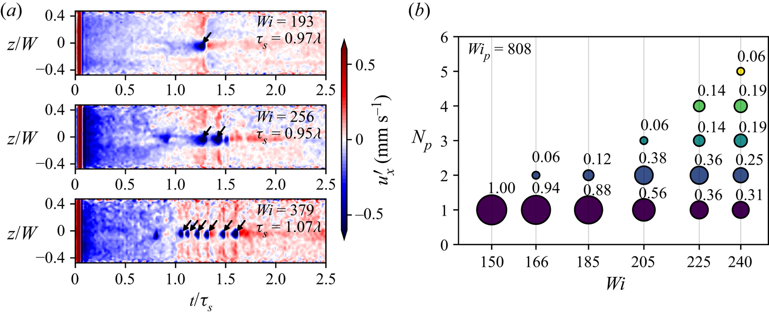
At higher  ${Wi}$, the response to perturbations changed since we observed groups of several pulses instead of the single downstream pulse. Examples for observations with multiple pulses are shown in figure 2(a) through space–time plots of the streamwise velocity fluctuations above the mean velocity profile, $u'_x$, for a roughly fixed value of ${De}^{-1}\approx 1$ and for three Weissenberg number values, ${Wi}=193$, $256$ and $379$; the pulses are highlighted with small arrows. For the ${Wi}=193$ case, a single downstream pulse, similar to that in figure 1(b), is observed at $t\approx 1.25\tau _s$. The pulse is localized at the centre of the channel, $z=0$, directly downstream to the injection hole. For the ${Wi}=256$ case, at least two downstream pulses are identified, and a third weaker one may be just evolving. Moreover, six pulses can be identified for the ${Wi}=379$ case. Therefore, we associate the observation that for a single-pulse constant perturbation there are multiple pulses downstream as a transition to a new state that can support pulse splitting.
(a) Space–time diagrams that demonstrate the streamwise velocity fluctuations about the mean velocity following localized perturbations at Weissenberg numbers close to and above the onset of pulse splitting. The flow is represented through contour plots of streamwise velocity fluctuations. The flow is perturbed at  $t=0$, and at approximately $t\approx \tau _s$ numerous pulses (one, two or six, depending on ${Wi}$) can be identified as localized low-velocity regions. Data are shown from three cases of roughly constant ${De}^{-1}$ and three ${Wi}$ values, with $S=188H$, $242H$ and $406H$, respectively. (b) A series of probability distributions for the number of downstream pulses counted in repetitions of the experiment, $N_p$. Each column of circles corresponds to a fixed ${Wi}$ case with a total of six cases, where ${Wi}_{{p}}=808$ is fixed. The area of each circle and the numbers printed correspond to the probability for observing $N_p$ for each ${Wi}$ value.
To investigate the transition to the new pulse-splitting state, we conducted measurements at various values of  ${Wi}$ and ${Wi}_{p}$ with numerous repetitions for each case. The results revealed that the response to our perturbations in the pulse-splitting regime was stochastic. Specifically, the number of downstream pulses observed varied seemingly at random from one experimental repetition to another even at fixed ${Wi}$, ${De}^{-1}$ and ${Wi}_{{p}}$. Therefore, we denote the number of pulses observed after an injection event as $N_p$ and estimate the dependence of its statistics on the control parameters at a fixed location in the channel, $S=483H$, while varying ${Wi}$ and ${Wi}_{{p}}$. For each value of the parameters, we used between 15 and 20 repetitions and gathered statistics of $N_p$. As an example, we show distributions of $N_p$ measurements for six values of ${Wi}$ in figure 2(b) for a fixed perturbation strength ${Wi}_{p} = 808$. While for ${Wi}=150$ only $N_p=1$ is observed in all repetitions, for ${Wi}=240$ the observed pulse count varied in the range $N_p \in ( 1 , 5 )$. This observation demonstrates that the pulse-splitting regime in our experiment was associated with a stochastic response to our perturbations.
Owing to the observed stochasticity, we characterize the transition to the pulse-splitting state through the ensemble average  $\langle N_p \rangle$. The dependence of $\langle N_p \rangle$ on ${Wi}$ is shown in figure 3(a) for six values of the perturbation strength, spanning slightly more than an order of magnitude of ${Wi}_{{p}}$. For fixed ${Wi}_{{p}}$ values, the average pulse count, $\langle N_p \rangle$, grows with ${Wi}$ above some critical value. Furthermore, for weaker perturbation strengths, $\langle N_p \rangle$ grows more slowly, and the transition seems to occur at higher values of ${Wi}$. Thus, using an empirical threshold of $\langle N_p \rangle _{Th} = 1.2$ to mark the transition to the pulse-splitting regime (shown as a dashed line in figure 3a), we denote the critical Weissenberg number for this crossing as ${Wi}_c$. As seen in figure 3(a), ${Wi}_c$ changes with the strength of the perturbation. Therefore, in the inset of figure 3(a) we plot $\langle N_p \rangle$ against the reduced Weissenberg number $({{Wi}}/{{Wi}_c}-1)$ for all values of perturbation strength, ${Wi}_p$. A least-squares fit to the data gives a scaling for the transition of $\langle N_p \rangle - \langle N_p \rangle _{Th} \propto ({{Wi}}/{{Wi}_c}-1)^\alpha$ with a scaling exponent of $\alpha = 1.33\pm 0.35$. Furthermore, we plot ${Wi}_c$ versus ${Wi}_{p}$ in linear scales in figure 3(b), showing the same data in log–log scales in the inset. Indeed, the perturbation strength value needed for the pulse-splitting transition decreases quickly with ${Wi}$; roughly an order of magnitude reduction in ${Wi}_{p}$ leads to a relatively modest change, only approximately 50 %, in ${Wi} _c$. Owing to the experimental uncertainty, a clear scaling is hard to obtain from the current data.
(a) The average number of pulses,  $\langle N_p \rangle$, observed at a distance of $S=486H$ downstream of the pulse injection location, shown as a function of the Weissenberg number. Data are shown for six levels of the pulse strength ${Wi}_{{p}}=60$, 121, 202, 404, 606 and 808. The inset shows the same data plotted against the reduced Weissenberg number, and a least-squares fit to the data gives a scaling exponent of $\alpha =1.33\pm 0.35$. (b) The pulse strength, ${Wi}_{{p}}$, required to obtain the critical Weissenberg number ${Wi}_c$, essentially showing the relation between the critical value for the transition and the perturbation strength. The inset shows the same data in log–log coordinates. The data and the error bars were calculated based on a linear interpolation of the data in panel (a).

4. Discussion and conclusions
In this work, we report the first experimental analysis of the viscoelastic channel flow response to localized perturbation for  ${Re}\ll 1$ and ${Wi}\gg 1$. Specifically, we perform an experiment in which we perturb the fluid in the channel with a single velocity pulse and observe the perturbed fluid downstream of the perturbation location. Our analysis shows a transition in the flow's response as ${Wi}$ is increased: for low ${Wi}$ we detect a single pulse that arrives at the downstream station; however, for higher ${Wi}$ we observe additional pulses and their numbers become random. Indeed, we observe a random number of pulses even though the same single perturbation event is produced; this indicates a transition to a pulse-splitting regime at sufficiently high ${Wi}$ and perturbation strengths. Importantly, such velocity pulses were not detected using a Newtonian fluid, which shows that this process is intrinsically related to the elasticity of the fluid.
An important observation is that the average number of pulses increases with  ${Wi}$. It is well known that polymer stretching and the elastic stress in viscoelastic channel flows grow with ${Wi}$ (for example, the base elastic stress grows as ${Wi}^2$ for the Oldroyd-B polymer model (Morozov & van Saarloos Reference Morozov and van Saarloos2007)). This suggests that the probability for pulse splitting to occur depends on the level of elastic stress in the fluid. This is also consistent with the observation that the critical value for the transition, ${Wi}_c$, decreases with the perturbation strength due to the stress related to the injection process.
The pulse-splitting regime in our experiment was stochastic since the number of pulses observed was random at fixed parameter values. A plausible explanation for the observed stochasticity may be that the base elastic stress in the channel fluctuates in time due to seemingly minor imperfections in the experimental apparatus. In particular, the presence of the injection cavity was seen to generate an elastic instability in the region close to the cavity, up to approximately  $S=200H$ (Shnapp & Steinberg Reference Shnapp and Steinberg2021). Then, a pulse-splitting event might occur when the elastic stress fluctuations become sufficiently strong. Notably, the current observations of the pulse-splitting regime were intentionally conducted very far downstream from the hole (e.g. $S=483H$ in figures 2b and 3a,b) at locations out of the direct influence of the hole-related instability. In any case, an elaborate modelling effort is required to fully resolve the details of the observed transition.
Our results indicate a new possible scenario for the growth of perturbations through an intrinsically elastic process. This observation is important since it suggests a plausible new route for the elastic instability and elastic turbulence to develop in viscoelastic channel flows. In addition, our new approach to the problem opens a new direction for continued research on this topic.
Acknowledgements
We are grateful to G. Han, R. Baron and G. Elazar for their assistance with the experimental set-up.
Funding
This work was partially supported by grants from the Israel Science Foundation (ISF; grant no. 882/15 and grant no. 784/19) and the Binational USA–Israel Foundation (BSF; grant no. 2016145). R.S. is grateful for the financial support provided by the Clore Israel Foundation.
Declaration of interests
The authors report no conflict of interest.


 Open access