Introduction

Glacier mass-balance modelling can be divided into accumulation and melt modelling. Both of these require accurate meteorological input data (e.g. precipitation and temperature). An essential problem in mass-balance modelling is the lack of available and accurate meteorological data. Small-scale meteorological conditions affecting snowfall in mountainous areas tend to vary significantly in both space and time, and point measurements on rocks or stations near glaciers may not be suitable for extrapolation to the glacier surface of interest. Air temperature, which is an important input variable for modelling, is easier to extrapolate over glacierized areas. By using assumptions concerning lapse rates and extrapolation techniques (e.g. Reference Gardner and SharpGardner and Sharp, 2009) it is possible to determine temperature fields to a higher degree of accuracy than precipitation.

Snow-depth observations and melt modelling have been used successfully to determine the snow water equivalent accumulation in previous studies in mountain areas (Reference Rango and MartinecRango and Martinec, 1982; Reference BagchiBagchi, 1983; Reference ClineCline, 1997; Reference Raleigh and LundquistRaleigh and Lundquist, 2009, Reference Raleigh and Lundquist2010). Others have used the snow depletion as validation of different mass-balance models (Reference Blöschl, Kirnbauer and GutknechtBlöschl and others, 1991; Reference Farinotti, Magnusson, Huss and BauderFarinotti and others, 2010). In this paper we explore a method that establishes an indirect relationship between temperature and peak accumulation (winter mass balance). We show that it is possible to estimate the winter accumulation from observed snow depletion data within the same accuracy range as for modelled summer melt. The input data needed are information on the snow-cover extent for one or multiple time-steps during the following melt season and air temperature. A required model parameter in the temperature-index melt model is a calibrated melt factor of snow. Calibration of the melt factor requires ablation stakes and snow density measurements. Transient snowlines can be used to improve the spatial distribution of the accumulation. Snowlines are readily detected in satellite images and aerial photographs and can be digitized with high precision (Reference Williams, Hall and BensonWilliams and others, 1991; Reference Turpin, Ferguson and ClarkTurpin and others, 1997) or they can be measured on the glacier.

The method of backward melt modelling, referred to here as ‘accumulation modelling’, is applied to an extensive meteorological and mass-balance dataset from Storglaciären, Sweden, for the year 2004. In this year transient snowlines were measured in the field using GPS on several occasions (Reference KootstraaKootstraa, 2005; Reference Hock, Kootstraa and ReijmerHock and others, 2007) and extensive probing and stake measurements were also carried out. Such data are only available for the year 2004. In addition, we have chosen this glacier for a number of other significant reasons: (1) there is an extensive mass-balance dataset for the glacier (Reference Holmlund and JanssonHolmlund and Jansson, 1999; Reference Holmlund, Jansson and PetterssonHolmlund and others, 2005; Reference ZempZemp and others, 2010); (2) hourly temperature and precipitation data are available from the nearby Tarfala Research Station (Reference Grudd and SchneiderGrudd and Schneider, 1996); (3) temperature-index modelling of the glacier has been conducted previously (Reference HockHock, 1999); and (4) the accumulation is highly influenced by the topography (Reference HulthHulth, 2006).

The relation between air temperature and glacier melt (Reference OhmuraOhmura, 2001; Reference Sicart, Wagnon and RibsteinSicart and others, 2005) has been used successfully to develop melt models based on a simple parameterization. Topographic features and solar geometry have been included to further enhance the classical temperature-index methods (e.g. Reference HockHock, 1999; Reference Pellicciotti, Brock, Strasser, Burlando, Funk and CorripioPellicciotti and others, 2005). Hock’s well-established temperature-index model is applied in this study.

Regression analysis, usually least-squares fitting of linear models, is also commonly used in mass-balance models to determine accumulation and it is of interest to determine whether the backwards melt modelling approach used here improves the results. A linear least-squares regression analysis on measured snow accumulation with elevation (87 mass-balance stakes) is conducted here and the results from both the accumulation model and the linear regression model are compared. Both methods are compared with the measured snow accumulation derived from kriging on 266 snow-probing points, measured independently of the 87 mass-balance stakes.

Accumulation Model

The accumulation model is based on the principle that it is easier to model melt spatially during the summer than to determine accumulation during the winter. Ablation is strongly related to positive air temperature and potential incoming solar radiation. Melt has been modelled previously on Storglaciären with an enhanced temperature-index model with good results (Reference HockHock, 1999). Accumulation on the other hand is highly influenced by the local meteorology and the topography since the snow is redistributed by wind after snowfall. Therefore it is difficult to model accumulation with a simple parameterization and it requires dense meteorology observations as input.

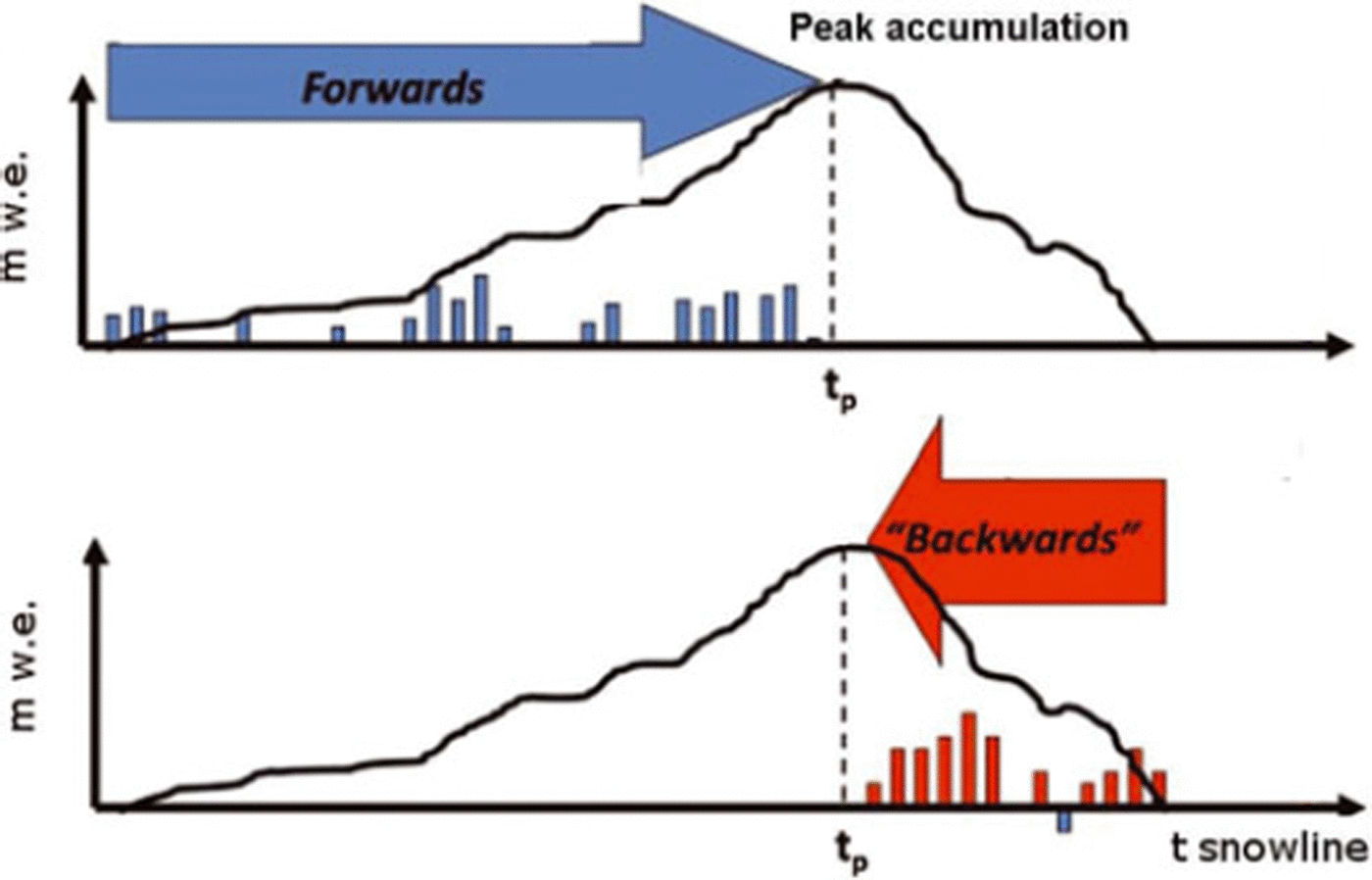
The accumulation is estimated using backwards calculations of the melt, applying a temperature-index model (Fig. 1). At the snowline location all snow from the previous winter has melted, while the ice melt has not yet started. If superimposed ice is insignificant, the snowline therefore corresponds to zero net mass balance. The total melt at a snowline from the beginning of the melt season to the snowline observation is calculated using the temperature-index model, and the result represents the peak winter accumulation along the snowline.

Fig. 1.

Illustration of the accumulation model. Vertical axis is calculated melt or accumulation (m w.e.). Horizontal axis is time, with peak accumulation at t_p and the timing of the snowline, t_snowline, marked. Blue bars illustrate precipitation events and red bars show melt events. Positive bars indicate addition in the direction of integration (forwards or backwards). Adapted from Reference Raleigh and LundquistRaleigh and Lundquist (2009).

The melt for the accumulation model is calculated applying a temperature-index model. Traditional models rely on a linear relation between melt and positive air temperature and are a good measure of average glacier melt. However, these models are restricted both spatially and temporally. Topographic effects such as surface slope, aspect and topographic shading introduce variation in melt rates. Therefore, we have chosen a temperature-index model that includes potential clear-sky radiation, which can be calculated without any additional meteorological input data, while introducing a spatial and temporal distribution of the melt rate considering topographic effects (Reference HockHock, 1999). This model was developed for Storglaciären but is generally applicable to glaciers of different sizes and located in a wide range of climatic conditions (Reference Hock, Johansson, Jansson and BarringHock and others, 2002; Reference Schuler, Melvold, Hagen and HockSchuler and others, 2005, Reference Schuler, Loe, Taurisano, Eiken, Hagen and Kohler2007; Reference Huss, Bauder, Werder, Funk and HockHuss and others, 2007).

A complete description of the melt model is provided by Reference HockHock (1999). However, we provide some information here. Melt M (mm h⁻¹) is calculated as

(1)

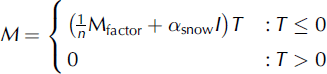
where n is the number of time-steps per day, Mf_actor (called MF in Reference HockHock, 1999) is a melt factor (mm d⁻¹ (°C)⁻¹), ä_{s n ow} (m² W⁻¹ mm h⁻¹ (°C)⁻¹) is a radiation coefficient for snow surfaces, I(Wm⁻²) is potential clear-sky direct solar radiation at the snow surface and T (°C) is air temperature. The calculation of the potential clear-sky radiation is described in Reference HockHock (1999), and through this term topographic effects such as slope, aspect and effective horizon and daily cycles of melt rates are included.

Data

Storglaciären (Fig. 2) is a polythermal glacier in northern Sweden at 67°54′10′′N, 18°34′0′′E. The glacier is about 3.5 km long and covers an area of 3.1 km² in the elevation range 1700–1150 m a.s.l.

Fig. 2.

Data for Storglaciären, 2004. Coloured lines indicate observed snowlines at the four different dates, and black dotted lines are elevation contours. Black dots show the 266 snow-probing points and grey squares the 87 ablation stakes.

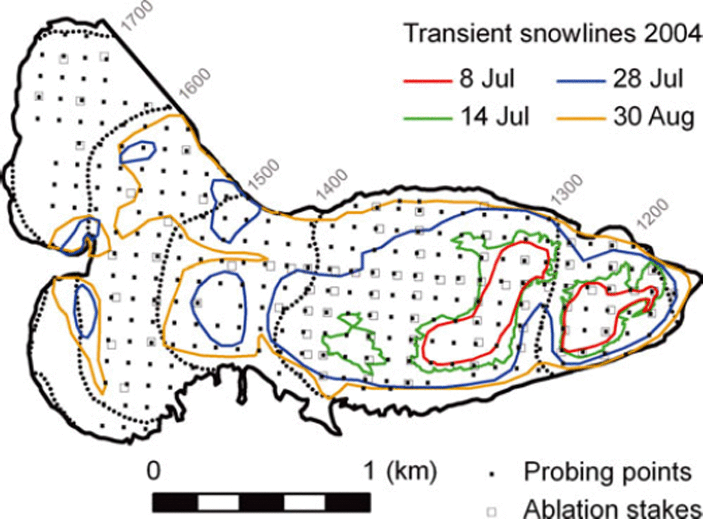
Snowlines were tracked by walking along the line of transition of snow to ice on seven occasions between 8 July and 30 August 2004 (Table 1; Fig. 2). Measurements were conducted with a handheld GPS unit with a horizontal accuracy of about 10m (Reference KootstraaKootstra, 2005).

Table 1.

Measurement dates of snowlines, snow depth and ablation on Storglaciären, 2004

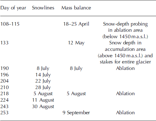
The winter snow accumulation was determined from 266 snow-probing points and snow density measurements at four pits conducted during two periods in spring 2004 (Reference KootstraaKootstraa, 2005). The ablation area, below 1450 m a.s.l., was measured from 18 to 25 April and the accumulation area, above 1450 m a.s.l., on 12 May (Table 1). The 266 snow-probing points were interpolated with regular kriging routines into a 30 m grid representing the snow accumulation of Storglaciären. The measured mean snow accumulation was 0.94 ± 0.10 mw.e.

The heights above the glacier surface of 87 stakes for the whole glacier were also measured on 12 May, 8 July and 5 August to determine melt (see Table 1). Melt is thus determined for three periods in the summer.

We use a digital elevation model (DEM) of Storglaciären from 1990 (Reference HolmlundHolmlund, 1996) with a 30 m × 30 m grid spacing.

Application

Calibration of the melt model

Melt was measured at 87 ablation stakes several times during the melt season (Table 1), and the net mass balances are calculated for three periods of the ablation season to provide input data for calibration of the temperature-index melt model (Fig. 2). Assumptions concerning summer snow density evolution are taken from a previous study on Storglaciären by Reference KootstraaKootstraa (2005). Snow density was assumed to vary with time according to the snow density curve measured on Storglaciären by Reference SchyttSchytt (1973), and this curve was used to assign snow densities to the dates when the stake measurements were carried out.

The model includes snow precipitation whenever the meteorological station records precipitation and the air temperature is below a threshold value of 0.5°C. A transition from solid to liquid precipitation mixture is used for the temperature interval 0.5–2.5°C, following Reference Hock and HolmgrenHock and Holmgren (2005). Air temperatures recorded at Tarfala Research Station (1130 m a.s.l.; Reference Grudd and SchneiderGrudd and Schneider, 1996) were extrapolated using a lapse rate of 0.58°C(100m)⁻¹ which drives the model. Snow is distributed evenly over the glacier surface, taking into account the extrapolated air temperature.

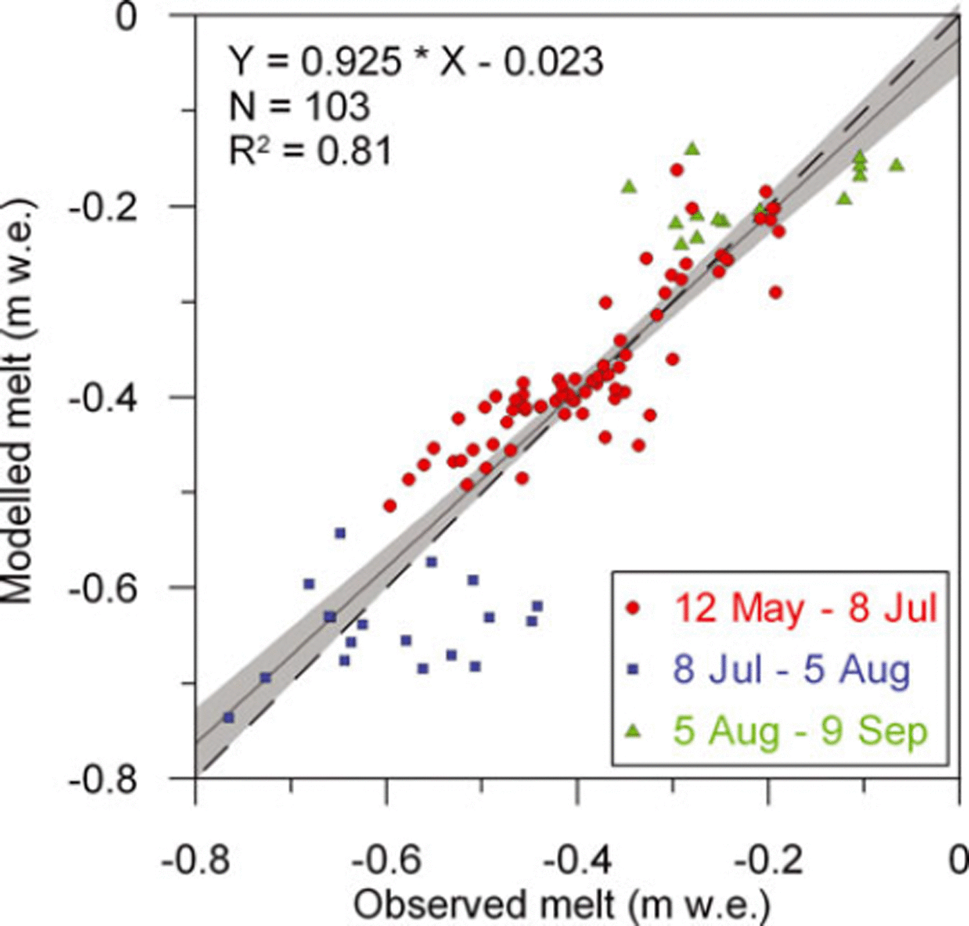
Calibration of the temperature-index model was achieved by optimizing the efficiency criterion, as described in Reference Nash and SutcliffeNash and Sutcliffe (1970), between observed and simulated cumulative snowmelt during three sub-periods between 12 May and 9 September (Table 1; Fig. 3). Optimal agreement was achieved by varying the melt factor, the radiation factor for snow and the lapse rate (Reference HockHock, 1999). A melt factor of Mf_actor = 1.48 (mm d⁻¹ (°C)⁻¹), a radiation factor of α_snow = 0.30 × 10⁻³ (m² W⁻¹ mm h⁻¹ (°C)⁻¹) and a lapse rate of 0.58°C(100m)⁻¹ gave the best agreement between observed and modelled cumulative melt for the entire period 12 May to 9 September. These optimal values are similar to those derived by Reference HockHock (1999) on the same glacier but for the year 1994. Figure 4 shows the sensitivity of the efficiency criteria, which is analogous to the coefficient of determination (R²), to variation in these parameters.

Fig. 3.

Calibration of melt model: 87 mass-balance stakes of observed and modelled melt for calibration in three periods (blue: winter to 8 July; red: 8 July to 5 August; green: 5 August to 17 September). Not all stakes were visited in every measurement period. The dashed black line indicates the 1 : 1 line. The thin solid black line with associated grey area indicates a linear regression fit to these data points and its uncertainty.

Fig. 4.

Sensitivity of the efficiency criteria (coefficient of determination, R²) to the three model parameters used for the melt model calibration: lapse rate, radiation factor and melt factor. Optimal values are centred in the plot, indicated by the vertical grey bar.

Snow accumulation linear regression model

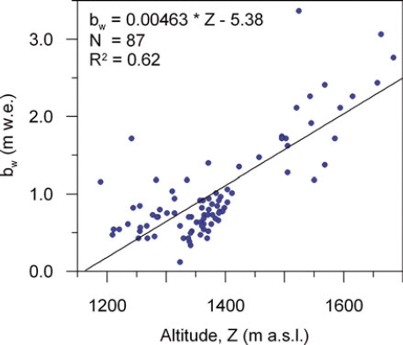
A snow accumulation gradient with elevation is derived using linear regression of observed accumulation with altitude at 87 mass-balance stakes (Fig. 5), independent of the 266 snow-probing points. The inclusion of surface slope, curvature and/or aspect did not improve the regression analysis.

Fig. 5.

Linear regression analysis of observed snow accumulation with elevation. The resulting fit is used to determine the linear regression accumulation model indicated in the figure. Measurements were carried out at 87 stakes on 12 May 2004.

Results: Modelled Accumulation

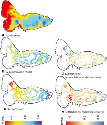
Observed and modelled accumulation along tracked snowlines is shown in Figure 6. Some measured snowlines have not been used for the assessment (at ∼1600 m) as they lay outside the probing and stake network. As seen in Figure 6d and e, the accumulation model reproduces the spatial distribution of snow better than the regression model. The regression model tends to over-predict the accumulation above 1400m while the accumulation model both under- and over-predicts in this area. The comparison with the observed winter accumulation also shows that the accumulation model reproduces the typical inhomogeneous snow distribution pattern of Storglaciären observed by Reference HulthHulth (2006).

Fig. 6.

Winter accumulations along tracked snowlines, modelled and observed, and differences (m w.e.). Grey lines are elevation contours. (a) Observed accumulation grid derived from kriging on 266 measured snow-probing points. (b) Results from the accumulation model. (c) Results from the linear regression model. (d) Difference between the accumulation model and observed winter accumulation. (e) Difference between the regression model and observed winter accumulation.

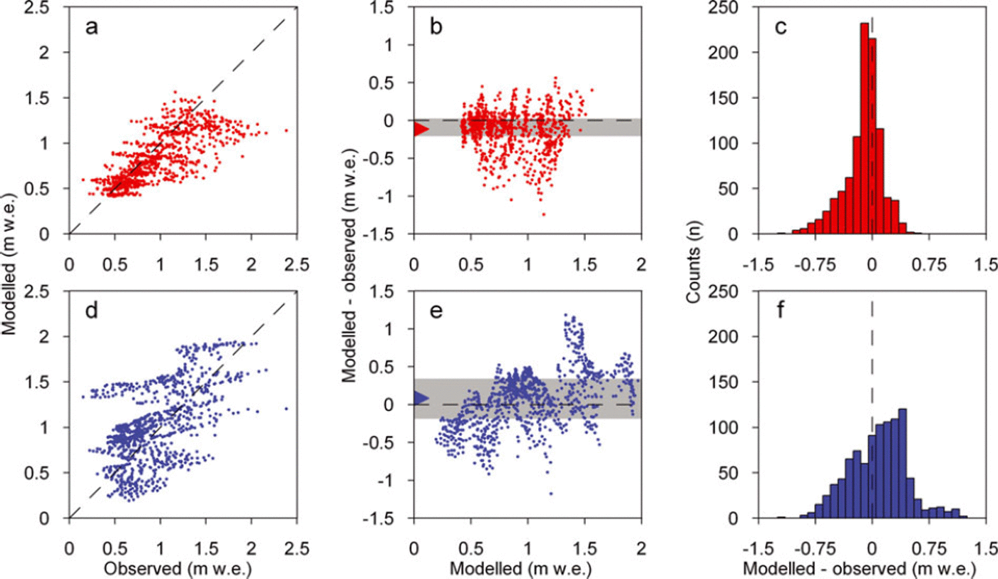
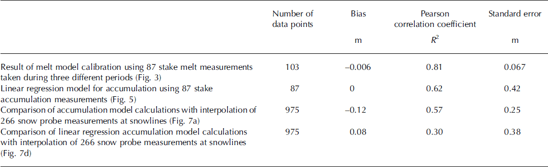
The accumulation model slightly underestimates the mean snowline accumulation by 10 cmw.e., and the regression analysis overestimates by 8 cm w.e. Standard deviation of the model residuals is significantly lower for the accumulation model than for the regression model, at 25 and 38 cmw.e., respectively. This is clear in the frequency distributions of the residuals (Fig. 7c and f).

Fig. 7.

Comparison of observed and modelled accumulation (mw.e.) using the accumulation and regression models at the gridcells along the tracked snowlines. Accumulation model: (a) observed versus modelled; (b) modelled versus difference (modelled – observed); (c) distribution of difference (modelled – observed) versus counts of gridcells (n). Regression model: (d) observed versus modelled; (e) modelled versus difference (modelled –observed); (f) distribution of difference (modelled – observed) versus counts of gridcells (n). In (b) and (e) the grey regions indicate the interquartile range and the triangles the mean of the model residuals.

Discussion

The uncertainties in the mean modelled winter accumulation relate primarily to the simplification of the physics in the temperature-index melt model; therefore, the modelled accumulation presented here will be at least as inaccurate as the results from the applied melt model. Uncertainties in snowline positions, presence of summer snowfalls and deviations from the assumption that the snowlines represent zero net balance also contribute to the total uncertainty in modelled winter accumulation. The contribution from the sum of these uncertainties in the snow accumulation modelling is assessed by comparison with observed data in this study.

In cases of summer snowfalls, the snowline position would move to a lower altitude on a subsequent date and the modelling concept would not be as applicable. Calculated melt would then be in periods of exposed ice instead of snow, which would lead to an incorrect calculation of accumulation. The presence of summer snowfall has to be considered through field observations or meteorological data when applying the method. For Storglaciären in summer 2004, when an extensive field campaign was conducted, the first snowfalls were reported on 17 September 2004 (Reference KootstraaKootstraa, 2005), which is after our calculation period.

The calculated accumulation is compared with observed accumulation derived from the interpolation of 266 snow-probing points; however, there is an uncertainty connected to these snow accumulation grid values. The observed values are based on point measurements of snow depth converted to mw.e. using density measurements, thereafter distributed by interpolation and extrapolation to cover the entire glacier surface. Mean snowline accumulation error is expected to be about 10 cm w.e., but specific point values are likely to exceed the mean error by several times. This is primarily due to errors related to unprobed areas and inhomogeneous areas (e.g. crevassed areas) and, to some extent, variations not registered by the relatively sparse observations of snow density (Reference JanssonJansson, 1999). The comparison of the calculated mean snowline accumulations deviates from the observed by –0.12mw.e. for the accumulation model and 0.08 mw.e. for the regression model. This is within the range of the estimated uncertainty.

Reference HulthHulth (2006) observed that the winter accumulation is highly influenced by topography. The linear regression analysis of the snow accumulation with elevation (Fig. 5) based on 87 mass-balance stakes yields a Pearson correlation coefficient of R ² = 0.62, which is lower than the correlation of the melt model (R ² = 0.81) using the same set of stakes during the melt season. This shows that the accumulation pattern is not only a function of elevation, but may be dependent on other factors such as local topography and wind. As a result, the spatial distribution of snow accumulation cannot be estimated very well using linear regression, as shown by the regression results in Figure 6e. Including snowlines and melt modelling improves the spatial pattern of the modelled snow accumulation, as shown in Figure 6d. The standard deviation of the comparison of modelled versus observed is also reduced from 0.38 m w.e. to 0.25m w.e. when applying the accumulation model at snowlines compared with the regression model, which shows that the spatial pattern of accumulation is better represented. The statistical results of the calibration and assessment of the model results are summarized in Table 2.

Table 2.

Summary of the statistical assessments presented in the text and figures

A limitation of the snow accumulation model is that it only provides estimates of the peak accumulation for the gridcells where we have observations of the transient snowline. However, snowlines are readily accessible from aerial photographs and satellite images for many glaciers around the globe. The recent trend of using time-lapse photography in glaciological studies makes this method even more useful when attempting to retrieve highly detailed snow accumulation estimates of specific glaciers. Even so, interpolation and extrapolation of the accumulation determined at snowlines is required for complete coverage of an accumulation area. Interannual variability of the accuracy of an interpolated accumulation grid is expected, since it will be dependent on the degree of melt and the spatial distribution and altitude of the snowlines for the specific season. There will also be varying results between glaciers, depending on the hypsometry of the glacier.

Conclusions

Snow accumulation data of glaciers are sparse. Field data are expensive and difficult to collect during winter seasons in remote areas, and the spatial distribution of snow accumulation varies locally. The purpose of this study is to develop and assess a method that can represent the spatial snow accumulation distribution and that requires minimum input data. In particular, the method can be applied without any available accumulation measurements. A temperature-index melt model is applied backwards (accumulation model), in combination with data on transient snowlines, to determine the winter snow accumulation along the snowlines. The following points have been addressed in this study:

1. 1. On-glacier observations of snowlines during the melt season have been used as a reference point for the accumulation modelling.

2. 2. Observed mean snow accumulation has been derived by interpolating 266 snow-probing points to the snowlines. The interpolated mean snowline accumulation was found to be 0.94 ±0.10mw.e. at observed snowlines.

3. 3. A temperature-index melt model has been calibrated using melt measurements from 87 independent stake measurements during the melt season, with a Pearson correlation coefficient of R² = 0.81.

4. 4. The accumulation model, using backward temperature-index melt modelling, has been applied at the snowlines, yielding an average modelled snowline accumulation of 0.82 ± 0.25 m w.e.

5. 5. A linear regression accumulation model based on altitude has been derived using 87 independent accumulation stake measurements, with a Pearson correlation coefficient of R ² = 0.62. Application of the regression model at the snowlines yields an average snowline accumulation of 1.02 ± 0.38 m w.e.

6. 6. The mean deviations between the observed and the modelled snowline accumulation lie within the range of the uncertainty of the measured data but the standard deviation is lower for the accumulation model than for the regression model. This, combined with the higher Pearson correlation coefficient of the accumulation model, indicates that the accumulation modelling method improves the spatial representation of the complex accumulation pattern of Storglaciären.

7. 7. The results also show that information on transient snowline locations can be usefully applied for the determination of the winter snow accumulation.