


1. Introduction
Flow-induced vibration (FIV), arising from the coupled interaction between a fluid and a structure (often termed fluid–structure interaction), is an important phenomenon prevalent in a great variety of engineering areas. Often observed as the swaying of large structures, such as bridges and high-rise buildings in strong winds as well as offshore platforms and oil risers in ocean currents, FIV is both detrimental in applications where structural failure or long-term fatigue is undesirable, and advantageous as a potential source of renewable energy (e.g. Wang et al. Reference Wang, Du, Zhao and Sun2017; Soti et al. Reference Soti, Zhao, Thompson, Sheridan and Bhardwaj2018; Lv et al. Reference Lv, Sun, Bernitsas and Sun2021). As such, the importance of FIV has motivated ongoing extensive research with the intention to characterise, predict and control FIV (e.g. Khalak & Williamson Reference Khalak and Williamson1996; Govardhan & Williamson Reference Govardhan and Williamson2000; Morse & Williamson Reference Morse and Williamson2009; Wong et al. Reference Wong, Zhao, Jacono, Thompson and Sheridan2017).
The FIV response of an elastically mounted bluff body in a cross-flow can typically be characterised by two distinct phenomena: vortex-induced vibration (VIV) and galloping. The VIV occurs as a result of the periodic shedding of vortices from an elastic or elastically mounted body in a pattern known as a vortex street, which in turn exerts unsteady fluid forces to cause the structural vibration. In general, VIV is characterised by its self-limited amplitudes due to the process of vortex shedding alternately from both sides of the body. On the other hand, galloping is driven by a movement-induced aerodynamic instability arising from the asymmetric pressure distribution caused by the changes in the instantaneous flow incidence angle as the body translates in the fluid (see Parkinson & Smith Reference Parkinson and Smith1964; Naudascher & Rockwell Reference Naudascher and Rockwell2005; Zhao et al. Reference Zhao, Leontini, Lo Jacono and Sheridan2014b, Reference Zhao, Nemes, Lo Jacono and Sheridan2018c). As both manifestations of FIV are dependent on the properties of the flow and the cylinder (e.g. flow velocity, Reynolds number, geometry, mass ratio, applied damping and structural stiffness), many past studies have chosen parameters such that VIV and galloping occur separately and can be individually investigated (Brooks Reference Brooks1960). However, more recent studies (see Nemes et al. Reference Nemes, Zhao, Jacono and Sheridan2012; Zhao, Hourigan & Thompson Reference Zhao, Hourigan and Thompson2018a) have shown that profound and complex fluid–structure interactions can also be observed when both VIV and galloping occur concurrently in an FIV system.
To date, while extensive investigations have been conducted on VIV of a circular cylinder (see Bearman Reference Bearman1984; Sarpkaya Reference Sarpkaya2004; Williamson & Govardhan Reference Williamson and Govardhan2004), much less attention has been given to FIV of elliptical cylinders. Herein, the cross-sectional profile of an elliptical cylinder is described by the elliptical ratio  $\varepsilon = b/a$, where $a$ and $b$ are the streamwise and cross-flow (transverse) dimensions, respectively. The circular cylinder, which is considered a special case of the elliptical geometry (with $\varepsilon = 1$), exhibits a pure VIV response in free stream flow due to the axial symmetry of the system; however, when the axial symmetry is broken, i.e. when $\varepsilon$ deviates from unity, the cylindrical body may become potentially susceptible to a movement-induced instability like galloping (see Naudascher & Rockwell Reference Naudascher and Rockwell2005). Few studies have been conducted on FIV of elliptical cylinders and even fewer on geometries with high $\varepsilon$. Leontini et al. (Reference Leontini, Griffith, Jacono and Sheridan2018) numerically investigated the influence of the angle of attack on both the FIV response and wake modes of an $\varepsilon = 1.5$ elliptical cylinder at a low Reynolds number of $\textit {Re} =100$. Here, the Reynolds number is defined by $\textit {Re} = U b/\nu$, where $U$ is the free stream velocity, and $\nu$ is the kinematic viscosity of the fluid. Hall (Reference Hall1984) demonstrated that the flow induced by a transversely oscillating elliptical cylinder is most unstable when $b>a$, in line with the numerical study of Navrose, Sen & Mittal (Reference Navrose, Sen and Mittal2014) which showed maximum vibration amplitude increases with $\varepsilon$ for a mass ratio of ${{m^{*}}} = 10.00$, and a Reynolds number and elliptical ratio range of $60\leq Re\leq 140$ and $0.7 \leq \varepsilon \leq 1.43$, respectively. This also concurred with the results obtained by Zhao, Hourigan & Thompson (Reference Zhao, Hourigan and Thompson2019a) who investigated the VIV of elliptical cylinders with mass ratio of ${{m^{*}}} = 6.00$ for an elliptical ratio range of $0.67\leq \varepsilon \leq 1.50$ at moderate Reynolds numbers ( $860 \leq {\textit {Re}} \leq 8050$). They found that the body vibration was enhanced, rather than attenuated, as the elliptical ratio was increased to $\varepsilon =1.50$; i.e. the afterbody was reduced for an elliptical cylinder. Note that the afterbody is defined as the structural part of a bluff body downstream of the flow separation points (see Brooks Reference Brooks1960; Bearman Reference Bearman1984; Zhao et al. Reference Zhao, Hourigan and Thompson2018a).
More recently, Vijay et al. (Reference Vijay, Srinil, Zhu, Bao, Zhou and Han2020) conducted a numerical study into the effect of the elliptical ratio, over the range  $1 \leq \varepsilon \leq 10$, as well as mass ratio, on the FIV response at low Reynolds number ( ${\textit {Re}} = 100$). In agreement with the results of Zhao et al. (Reference Zhao, Hourigan and Thompson2019a), the largest elliptical ratio was found to incite the highest amplitude response, approximately twice the amplitude observed for the case of the circular cylinder under identical conditions.
In summary, studies in the literature have shown that the FIV behaviour of a bluff body is strongly dependent on the geometric properties and flow conditions, such as geometric shape, afterbody, structural damping ratio, reduced flow velocity and Reynolds number. However, the effect of structural damping on the FIV response of large-elliptical-ratio geometries at moderate Reynolds numbers that can sustain the very large amplitude oscillations remains poorly understood. Filling this gap in the literature could have profound implications in the field of renewable energy generation, where the maximum amount of power extracted by the system can be considered as an optimisation problem between two negatively correlated parameters: structural damping and oscillation amplitude. A recent example is the VIVACE (VIV aquatic clean energy) converter, pioneered by Bernitsas et al. (Reference Bernitsas, Raghavan, Ben-Simon and Garcia2008), which demonstrated that VIV of a circular cylinder is a viable method of extracting renewable energy from bodies vibrating naturally in flowing fluids. However, as a result of the circular cylinder VIV being self-limited to one body diameter and within discrete ranges of flow speeds, many studies have investigated optimal experimental parameters (e.g. surface modifications (Ding et al. Reference Ding, Zhang, Bernitsas and Chang2016), geometries that undergo galloping (Tamimi et al. Reference Tamimi, Seif, Shahvaghar-Asl, Naeeni and Zeinoddini2019) and structural properties (Lee & Bernitsas Reference Lee and Bernitsas2011; Soti et al. Reference Soti, Zhao, Thompson, Sheridan and Bhardwaj2018)) to maximise the energy harvesting performance. Whilst the current progress on applying FIV for hydrodynamic energy generation has been aptly reviewed by Lv et al. (Reference Lv, Sun, Bernitsas and Sun2021), no study on the utilisation of elliptical cylinders for power extraction to date has addressed flow conditions and geometric parameters conducive to very high oscillation amplitudes. As such, a further understanding of the impact of damping on the FIV of elliptical geometries, especially one with unprecedented amplitudes at relatively low reduced velocities, could pave the way for more efficient methods of energy generation based on this approach.
This study presents a comprehensive investigation into the influence of structural damping on FIV of a thin elliptical cylinder with an elliptical ratio of  $\varepsilon = 5$. The study aims to experimentally elucidate the FIV response of a thin elliptical cylinder as a function of reduced velocity over a wide range of structural damping ratios ( $3.62\times 10^{-3}\leq \zeta \leq 1.87\times 10^{-1}$) at moderate Reynolds numbers.
The article proceeds by outlining the experimental method in § 2. The amplitude response as well as frequency contours of the displacement and fluid forces are presented in § 3.1. Section 3.2 describes the fluid forces and their phases relative to the body displacement, followed by an analysis of the observed wake modes in § 3.3 to understand the complex fluid–structure interaction that causes these substantially large oscillations. Finally, the conclusions are drawn in § 4, highlighting the important findings and the significance of the current study.
2. Experimental method
2.1. Fluid–structure system modelling
Figure 1 depicts the schematic of an elliptical cylinder undergoing FIV, which is constrained with one degree of freedom to oscillate transversely to the free stream flow. The system dynamics can be described by a simplified second-order governing equation for a linear mass–spring–damper oscillator,
 \begin{equation} m\ddot{y}(t)+c\dot{y}(t)+ky(t) = F_{y}(t), \end{equation}
where  $m$ is the total oscillating mass, $c$ is the structural damping, $k$ is the spring constant, $y$ is the cylinder displacement and $F_{y}$ is the transverse fluid forcing term, noting that the over-dot symbols represent derivatives with respect to time ( $t$). Table 1 shows the relevant non-dimensional parameters for the study.
(a) A schematic defining the problem of interest: an elastically mounted elliptical cylinder model constrained to oscillated transverse ( $y$) to the free stream flow of velocity $U$, which is in the positive $x$ direction. Here, the geometry is characterised by the elliptical ratio $\varepsilon = b/a$, where $a$ and $b$ are the streamwise and cross-flow dimensions, respectively. Additionally, $m$ is the oscillating mass, $k$ denotes the spring constant, $c$ is the adjustable structural damping and ${{F_{x}}}$ and ${{F_{y}}}$ represent the drag and the transverse (lift) fluid forces acting on the body, respectively. (b) A photograph showing the experimental set-up used in the present study.

Relevant non-dimensional parameters. Here,  $A$ is the vibration amplitude in the $y$ direction, ${{m_{d}}}$ is the displaced mass of the fluid, ${{m_{A}}}$ is the added mass, $\nu$ is the kinematic viscosity of the fluid, ${{f_{{nw}}}}$ is the natural frequency of the system in quiescent water, $\,{f_{{St}}}$ is the fixed-body vortex shedding frequency, $L$ is the immersed length, $\rho$ is the fluid density and $f_y$ is the body oscillating frequency. Here $F_y, F_v$ and $F_x$ are the transverse lift, vortex and streamwise drag forces, respectively, with the corresponding frequency for each term being $f_{C_y}, f_{C_v}$ and $f_{C_x}$.

The present experiments were undertaken in the free-surface recirculating water channel of the Fluids Laboratory for Aeronautical and Industrial Research (FLAIR) at Monash University. The water channel has a test section of 4000 mm in length, 600 mm in width and 800 mm in depth. The mass–spring–damper system was modelled based on a low-friction air-bearing rig, which was placed atop the water channel working section and transverse to the free stream flow direction. Further details on the platform and the air-bearing rig used in the current study can be found in Zhao et al. (Reference Zhao, Hourigan and Thompson2018a,Reference Zhao, Jacono, Sheridan, Hourigan and Thompsonb). The test elliptical cylinder was manufactured from aluminium and had streamwise and cross-flow (transverse) dimensions of  $a = 5\pm 0.10\ {\rm mm}$ and $b = {25 \pm 0.10}\ {\rm mm}$, respectively, resulting in an elliptical ratio of $\varepsilon = 5$. The immersed length of the cylinder was ${614\pm 0.50}\ {\rm mm}$ with an aspect ratio of $AR = L/b = 24.6$. To promote parallel vortex shedding through the attenuation of end effects, an end-conditioning platform was positioned approximately 1 mm ( $4$ % of $b$) below the free end of the cylinder (see Khalak & Williamson Reference Khalak and Williamson1996). The use of the platform to reduce end effects has been validated and utilised extensively by Zhao et al. (Reference Zhao, Leontini, Lo Jacono and Sheridan2014b, Reference Zhao, Jacono, Sheridan, Hourigan and Thompson2018b), Wong et al. (Reference Wong, Zhao, Jacono, Thompson and Sheridan2017) and Soti et al. (Reference Soti, Zhao, Thompson, Sheridan and Bhardwaj2018).
The total oscillating system mass was  $m = {1046.4}\ {\rm g}$ and the mass of the displaced water was $m_d = \rho {\rm \pi}abL/4 = {60.0}\ {\rm g}$, giving a mass ratio of ${{m^{*}}} = m/m_d = 17.4$. The spring constant was provided by a pair of precision extension springs. The structural damping was controlled using an eddy-current magnetic damper mechanism developed by Soti et al. (Reference Soti, Zhao, Thompson, Sheridan and Bhardwaj2018). The desired damping was achieved by adjusting the gap ( $G$) between the magnet and copper plate, via a microdrive stage with a resolution of 0.01 mm.
Free-decay tests were conducted individually in both air and quiescent water to determine the natural frequency of the system and structural damping ratios. The system characteristics were described using the structural damping ratio with added mass in potential flow ( ${{m_{A}}}$) considerations, which is defined as $\zeta = c/(2\sqrt {k (m + {{m_{A}}})})$. In practice, this can be determined experimentally through the relationship ${{m_{A}}} = ({({{f_{{na}}}}/{{f_{{nw}}}})}^2-1)m$, which in turn is dependent on the natural frequencies in both air ( ${{f_{{na}}}}$) and water ( ${{f_{{nw}}}}$). As the damping force exerted by the damper mechanism is controlled by the gap, $G$, figure 2 shows the variations in $\zeta$, ${{f_{{na}}}}$ and ${{f_{{nw}}}}$ with the gap distance.
(a) Structural damping  $\zeta$ and (b) natural frequencies as a function of the gap ( $G$) between the magnet and copper plating of the electromagnetic damper system developed by Soti et al. (Reference Soti, Zhao, Thompson, Sheridan and Bhardwaj2018). Panels (bi) and (bii) denote the respective natural frequencies in both air, ${{f_{{na}}}}$, and water ${{f_{{nw}}}}$.

It should be noted that in the present study, streamwise drag and the transverse lift are described in dimensionless forms defined by  $C_{x} = F_{x}/(\rho U^2bL/2)$ and $C_{y} = F_{y}/(\rho U^2bL/2)$, respectively, where $\rho$ is the fluid density, and $L$ is the immersed length of the cylinder. In addition, the dimensionless form of the vortex force is given by $C_{v} = F_{v}/(\rho U^2bL/2)$, which was computed through a decomposition of the total transverse force into a vortex force component ( $F_v$) and a potential force component ( $F_P$), namely $F_y = F_v + F_P$. Note that the potential force (in an inviscid fluid) is given by $F_{P} =-m_{A}\ddot {y}$, with $m_A$ being the added mass (see Govardhan & Williamson Reference Govardhan and Williamson2000; Morse & Williamson Reference Morse and Williamson2009; Zhao et al. Reference Zhao, Leontini, Jacono and Sheridan2014a,Reference Zhao, Leontini, Lo Jacono and Sheridanb).
2.2. Data acquisition and processing
The control of the free stream velocity as well as data acquisition (DAQ) were automated through customised LabVIEW (National Instruments, USA) software with measurements taken using a USB DAQ device (model USB6218-BNC; National Instruments, US) sampling at 100 Hz for 300 s. Transverse displacement was measured using a non-contact digital optical linear encoder (model RGH24; Renishaw, UK) with a range of  $\pm {200}\ {\rm mm}$ at a resolution of ${1}\ {\mathrm {\mu }}{\rm m}$, whilst the transverse force ( ${{F_{y}}}$) was obtained based on (2.1) where the first- and second-order derivatives were determined through numerical differentiation of the displacement signal (see e.g. Sareen et al. Reference Sareen, Zhao, Lo Jacono, Sheridan, Hourigan and Thompson2018). The drag force ( ${{F_{x}}}$) was directly measured using a two-component force balance based on semiconductor strain gauges arranged in a Wheatstone bridge configuration.
The fluid–structure interaction between the fluid flow and elliptical cylinder was investigated over the structural damping ratio range  $3.62 \times 10^{-3} \leq \zeta \leq 1.87\times 10^{-1}$, encompassing a variation by a factor of $\sim 50$, for reduced velocities of $2.3 \leq U^* = U/({{f_{{nw}}}} b) \leq 10$. The free stream velocity range tested was $40 \leq U \leq {180}\ {\rm mm}\ {\rm s}^{-1}$, corresponding to the Reynolds number range $980 \leq \textit {Re} \leq 4410$, where $\textit {Re} = Ub/\nu$ with $\nu$ being the kinematic viscosity of the fluid. The free stream turbulence level was less than 1 % over the flow velocities of interest. To further test the mechanism of movement-induced vibration as well as the hysteresis effect in transitions between different FIV response regimes, experiments of both increasing and decreasing reduced velocities were conducted.
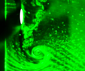
To visualise the wake structures responsible for the oscillations of the elliptical bluff body, particle image velocimetry (PIV) was employed to image through the cross-sectional plane of the cylinder. After seeding the flow with hollow microspheres (model Sphericel 110P8; Potters Industries Inc.) of normal diameter  ${13}\ {\mathrm {\mu }}{\rm m}$ and specific weight ${1.10}\ {\rm g}\ {\rm cm}^{-3}$, the images were captured with a high-speed camera (Dimax S4; PCO AG, Germany) with resolution $2016 \times 2016\ {\rm pixel}^2$ and equipped with a 50 mm lens (Nikon Corporation, Japan). The optical magnification factor was approximately ${6.23}\ {\rm pixel} \ {\rm mm}^{-1}$. Illumination was provided by a 3 mm thick laser sheet from a 5 W continuous laser (model MLL-N-532 nm-5W; CNI). For each trial, a set of 3100 image pairs was recorded at a sampling rate of 10 Hz. Validated in-house software, originally developed by Fouras, Jacono & Hourigan (Reference Fouras, Jacono and Hourigan2008), was then used to correlate $32 \times 32$ pixel2 interrogation windows with 50 % window overlap to obtain the time-dependent vector fields of the wake flow. Finally, the resultant fields were phase averaged by dividing them into 48 phases based on the cylinder displacement and velocity, and averaging over each bin (see Zhao et al. Reference Zhao, Jacono, Sheridan, Hourigan and Thompson2018b).
3. Results and discussion
3.1. Structural vibration response
Figure 3 shows the normalised amplitude response of the elliptical cylinder of  $\varepsilon = 5$ as a function of reduced velocity for a range of structural damping ratios. Note that the normalised amplitude is defined by $A^{*} = A/b$, with $A$ being the dimensional vibration amplitude for a given reduced velocity, and ${{A^{*}_{{10}}}}$ represents the mean of the top 10 % of amplitude peaks (see Nemes et al. Reference Nemes, Zhao, Jacono and Sheridan2012; Zhao et al. Reference Zhao, Leontini, Lo Jacono and Sheridan2014b, Reference Zhao, Hourigan and Thompson2019a). In this study, measurements with increasing and decreasing $U^*$ are displayed by unfilled and solid markers, and denoted by $U^* \! \uparrow$ and $U^* \! \downarrow$, respectively. In this figure, the amplitude responses are plotted in two subplots: figure 3(a) for responses displaying a hyper branch (i.e. $\zeta \leq 1.88 \times 10^{-2}$) and figure 3(b) for responses without the appearance of a hyper branch.
Normalised amplitude response ( ${{A^{*}_{{10}}}}$) for the elliptical cylinder of $\varepsilon = 5$ as a function of reduced velocity for various structural damping ratios ( $\zeta$). The cases with the presence of hyper branch are plotted in (a), whilst the other cases with the absence of hyper branch are shown in (b). Note the difference in the ranges of ${{A^{*}_{{10}}}}$ for the two subfigures.

It should also be noted that the vibration amplitude would exceed the limit of the air-bearing rig ( $A^* \approx 8$) for $\zeta \leq 1.88 \times 10^{-2}$ when $U^*$ was increased beyond $8$. To prevent the growing amplitude cylinder from hitting the physical limit of the air-bearing rig, the flow was set to zero velocity when the vibration amplitude was close to the limit (at $U^* \approx 7.6$) via the LabVIEW data acquisition program. After this temporary stop, the flow velocity was resumed from rest to sweep through the rest of the programmed $U^*$ values (in an increment of 0.05 or 0.1). This procedure could prevent the occurrence of ‘hard’ movement-induced FIV response (one that requires a ‘hard’ trigger, as discussed in Zhao et al. (Reference Zhao, Hourigan and Thompson2018a)), and thus the FIV responses in figure 3(a) fall onto a lower branch for $U^* \gtrsim 7.6$. Thus, it is not clear how much further the hyper branch response would continue beyond this water-channel based $U^*$ limit.
3.1.1. The FIV response regimes
For increasing and decreasing  $U^*$ trends, figures 4 and 5, respectively, present the normalised power spectral density (PSD) contours of the body vibration frequency ( $\,{f^{*}_y}$) and transverse lift frequency ( $\,{f^*_{C_y}}$) as a function of $U^*$ for selected $\zeta$ values. Note that the frequency components are normalised by ${{f_{{nw}}}}$; i.e. $\,{f^{*}_y} = f_y /{{f_{{nw}}}}$ and $\,{f^*_{C_y}} = f_{C_y} / {{f_{{nw}}}}$. Further details of the construction method for the PSD contours can be found in Zhao et al. (Reference Zhao, Leontini, Lo Jacono and Sheridan2014b). Whilst the vortex-force frequency responses appeared identical to those of $\,{f^*_{C_y}}$ in the present experiments, their PSD contours are not provided in our current study.
(ai–aii) The normalised amplitude response (increasing  $U^*$) and logarithmic-scale PSD contours of the (bi–gi) normalised vibration ( $\,{f^{*}_y}$), and (bii–gii) transverse fluid force ( $\,{f^*_{C_y}}$) frequencies as a function of $U^*$ for selected $\zeta$ values from figure 3. In (b–g), the horizontal dashed line highlights the frequencies at $\,{f^{*}} \in \{1,2,3\}$; the vertical dashed lines represent the boundaries of different response regimes (i.e. I, II, hyper branch (H), III and desynchronisation (D)); and the dot–dashed line represents the Strouhal frequency measured for a stationary cylinder.

(ai–aii) The normalised amplitude response (decreasing  $U^*$) and logarithmic-scale PSD contours of the (bi–gi) normalised vibration ( $\,{f^{*}_y}$) and (bii–gii) transverse fluid force ( $\,{f^*_{C_y}}$) frequencies as a function of $U^*$ for selected $\zeta$ values from figure 3. More details can be found in the caption of figure 4.

As shown in figures 4 and 5, the FIV response can be categorised by four distinct synchronisation (or ‘lock-in’) regimes and a desynchronised region. These domains were classified based on an overall evaluation of the amplitude and frequency responses, as well as the fluid forces and their phases relative to the body displacement. The lock-in regions are labelled I, II, H (hyper branch) and III, according to the characteristics of the response at low damping. As discussed in detail below, these labels are drawn from commonality in both the amplitude response, and the displacement and lift coefficient frequency response across damping ratios. Sample time traces of the body displacement ( $y^*$), the fluid forces (represented by their coefficients $C_x$ and $C_y$), and the total phase ( $\phi _t$) selected from each synchronisation regime are also shown in figure 6 to illustrate the periodic dynamics.
Sample time traces of the cylinder vibration for the minimum damping ratio tested ( $\zeta = 3.62\times 10^{-3}$) at different reduced velocities selected from the four synchronisation regimes: (a) $U^* = 3.0$ (I); (b) $U^* = 4.0$ (II); (c) $U^* = 6.0$ (hyper branch); and (d) $U^* = 8.0$ (III). Note that the total phase $\phi _{t}$ (the relative phase of $C_y$ with respect to $y^*$) is shown in degrees, and the time is normalised ${{f_{{nw}}}}$, namely $\tau = t{{f_{{nw}}}}$.

To quantify the effect that hysteresis and damping have on the FIV of the elliptical cylinder, the response at the minimal damping ratio tested ( $\zeta = 3.62 \times 10^{-3}$) for increasing $U^*$ will be described in detail here and used as a baseline in later parts of the section to highlight the effects of $U^*$ direction and increased $\zeta$ values on the resultant dynamic responses.
In the present study for the baseline case (figure 4b), the first regime (regime I) occurs over a reduced velocity range of  $U^* \lesssim 3.2$, where a wake–body synchronisation (represented by the matching of the dominant frequencies of $\,{f^{*}_y}$ and $\,{f^*_{C_y}}$) is clearly present, occurring at ${{f_{{nw}}}}$. It should be noted that the fluid forcing frequency also sees a weak second harmonic component (i.e. $\,{f^*_{C_y}} \simeq 2$). In this regime, the amplitude response ${{A^{*}_{{10}}}}$ exhibits an almost linear growth with increasing $U^*$. In regime II (over $3.2 \lesssim U^* \lesssim 4.8$), the ${{A^{*}_{{10}}}}$ response continues the linear growth trend as in regime I. However, in addition to a second harmonic in $\,{f^*_{C_y}}$, a third harmonic also develops as shown in figure 4(bii).
As  $U^*$ is further increased to regime H (the hyper branch regime over $4.8 \lesssim U^* \lesssim 7.05$), the beginning of the hyper branch is marked by a sudden jump in ${{A^{*}_{{10}}}}$ but with a small step-like decrease in the third harmonic of $\,{f^*_{C_y}}$. Similar to the upper branch of the VIV response for a circular cylinder, the hyper branch regime is featured by the largest-scale body oscillation amplitudes for this damping case ( ${{A^{*}_{{10}}}}$ up to $7.7$ at $U^* = 7.05$ prior to a temporary reset of the flow velocity to zero). It is important to highlight that the upper limit of this regime is artificial since the flow velocity was deliberately reset to zero when the body vibration approached the limit of the experimental rig, as discussed above. Due to the largest-scale amplitudes in this regime being driven by the ‘hard’ movement-induced instability, allowing the cylinder to return to rest before the flow was restarted causes the premature onset of regime III (lower branch). This sees its ${{A^{*}_{{10}}}}$ value decreasing to 0.967, $12.6\,\%$ of the peak value of hyper branch (figure 3a). As such, the onset of ‘true’ transition from hyper branch to lower branch, which is solely dependent on the ‘natural’ response of the FIV system alone, will occur at higher $U^*$.
Occurring over  $7.05 \lesssim U^* \lesssim 8.10$ with a maximum amplitude of ${{A^{*}_{{10}}}} \simeq 0.967$, regime III is analogous to the lower branch in VIV of the circular cylinder response and corresponds to a monotonically decreasing ${{A^{*}_{{10}}}}$ trend with increasing $U^*$. The fall in body vibration amplitude also coincides with an increase in the body and transverse fluid force frequencies to $1.06{{f_{{nw}}}}$ (figure 4b). Meanwhile, the contribution of the second and third harmonics to the frequency response of the $y$-direction fluid force becomes negligible in this regime. Unlike the frequency response in the hyper branch, the harmonic frequency in regime III gradually increases with $U^*$.
Outside the four synchronisation regimes, the fluid–structure interaction becomes desynchronised as the frequency response of the transverse lift becomes a broadband centred about a main signal at the Strouhal vortex shedding frequency,  $\,{f_{{St}}}$ (figure 4b). The same contribution was also observed in the body vibration PSD contours, as well as an additional broadband signal close to the natural frequency of the system in water. Note that the Strouhal number was experimentally measured to be ${\textit {St}} = {f_{{St}}} b/U = 0.169$ for the stationary cylinder case.
3.1.2. Hysteresis effects in the amplitude response
We will now address the effect of changing the direction of the  $U^*$ increments on the amplitudes and lock-in response regimes (see figure 5 for PSD contours). In relation to the baseline case ( $U^*$ is increased, $\zeta = 3.62 \times 10^{-3}$), the hysteretic nature of the observed FIV phenomena can be investigated through comparisons with data obtained for the same damping ratio but with decreasing $U^*$ increments. Whilst the peak amplitude over the tested $U^*$ range for both increment directions follows a typical three-branch response, the reduced velocity ranges in which these regions occupy differ. This is most apparent in the transition between the hyper branch and regime III, which occurs at a lower value of $U^* = 6.15$ for decreasing increments as compared with $7.05$ for the baseline case. As such, the reduced $U^*$ value results in a smaller maximum hyper branch response ( ${{A^{*}_{{10}}}}\simeq 5.99$) and an increased maximum lower branch-like (regime III) response ( ${{A^{*}_{{10}}}}\simeq 2.42$) relative to the baseline. Therefore, the hysteretic behaviour indicates that the hyper branch regime is dependent on the initial state of the elliptical cylinder system (i.e. the oscillation amplitude), and explains why the direction of the $U^*$ increment will determine the manifestation of either regime III or the hyper branch for intermediate reduced velocities ( $U^* = 6.2$– $7.05$). The movement-induced nature of the hyper branch, which is the cause of this hysteresis, will be further discussed in § 3.3. Furthermore, the presence of a weak second-harmonic component, undetected when $U^*$ was increased and the strength of which increases as the transition to the hyper branch is approached, was also observed in the transverse fluid forces of regime III (figure 5bii).
Aside from the aforementioned aerodynamic instability regime, hysteresis was also present in the boundary between the desynchronisation and third regimes, with the onset of the former region occurring for a lower reduced velocity of  $U^* = 7.8$. Regime III can be considered predominantly VIV in nature due to its similarities to the lower branch of the circular cylinder amplitude response, as well as an absence of higher harmonic contributions to the ${{C_{y}}}$ frequency contours in this region (refer to § 3.2 for further justification). As such, the observed hysteresis phenomenon can be attributed to the effect of transverse cylinder oscillations on the after-body wake structure (Blevins Reference Blevins1990). In the case when $U^*$ was increased, the amplitude response of regime III likely prolonged the synchronisation of the wake and body to the natural frequency and hence delayed the desynchronisation to higher reduced velocities as compared with the reverse $U^*$ direction.
3.1.3. Impact of structural damping on the overall dynamic response
The question now arises as to how increasing  $\zeta$ from the minimum value tested (baseline case) affects the FIV characteristics of the elastically mounted elliptical cylinder. Figure 7, a two-dimensional contour plot of figure 3, indicates the variation of the synchronisation regimes in the $U^*$– ${A^{*}}$ parameter space as a function of $\zeta$. This effect can be categorised into two $\zeta$ domains: $\zeta \leq 1.88\times 10^{-2}$ where the hyper branch regime is present (figure 3a); and $\zeta \geq 1.92\times 10^{-2}$ with the absence of the hyper branch response (figure 3b). Though not the focus of this study, the boundaries of the FIV response regimes shown in figure 7 can also be affected by the value of the Reynolds number.
The normalised amplitude contours plotted in  $U^*$– $\zeta$ space. Based on an overall examination of the vibration amplitude and frequency responses as well as fluid forcing phases, the FIV response is characterised by five different regimes: regime I; regime II; hyper branch; regime III; and the desynchronised region. The approximate boundaries of each region are marked by the dashed lines. The overlaid crosses denote the damping and reduced velocity values at which spot PIV measurements were taken, with the red crosses representing the locations of the PIV contours as further discussed in § 3.3. Panel (a) corresponds to $U^*$ increasing, and panel (b) to $U^*$ decreasing.

As indicated by figure 3(a), increasing the structural damping of the system results in an overall delay in the onset of all four lock-in regimes to higher  $U^*$ values. An additional desynchronisation region for which the $U^*$ range expands with $\zeta$, emerged on the left of regime I. Hysteresis, due to the same reasoning applied to the VIV-dominated regime III, also occurs to the transition between the desynchronisation region and regime I. As such, the $U^*$ value for which the transition occurs increases with $\zeta$ for both $U^*$ increment directions.
Whilst the damping-induced delaying effect is especially noticeable in the onset of regimes I and II as well as in the hyper branch, the same retardation in  $U^*$ with increased $\zeta$ is minimal for regime III as evidenced by the general concurrence in amplitude across all damping ratios below $\zeta = 1.88\times 10^{-2}$ (figure 3a). The main source of deviation was observed near the boundary between regime III and the hyper branch for decreasing $U^*$, with higher $\zeta$ resulting in the curvature of the lower branch-like amplitude response being less pronounced. Along with the delay in the onset of the hyper branch regime, the increase in damping ratio for decreasing $U^*$ increments also leads to a reduction of the maximum amplitude in the regime.
For the third harmonic components in the transverse fluid forces observed for regime II of the baseline case, increasing the damping ratio caused an overall decrease in both the strength of the harmonics (see figures 4b, 4c, 5b and 5c) as well as the overall  $U^*$ range of the lock-in region (figure 7). As this decrease in higher-order frequency components also corresponds to the delay of the amplitude response of the four lock-in regions (i.e. a higher $U^*$ value required to attain a given ${{A^{*}_{{10}}}}$), the presence of the harmonic components may be important in the development of large transverse oscillations in the system. This conclusion concurs with the suggestions made by Zhao et al. (Reference Zhao, Leontini, Lo Jacono and Sheridan2014b) and Wang et al. (Reference Wang, Du, Zhao and Sun2017) for transverse FIV, and Zhao et al. (Reference Zhao, Jacono, Sheridan, Hourigan and Thompson2018b) for in-line FIV, where large-scale body vibrations were attributed to the harmonic synchronisations in the fluid forces. However, an exception to the above generalisations was observed during the transition from regime III to the hyper branch for decreasing $U^*$, where the $\,{f^{*}} =3$ contribution to $\,{f^*_{C_y}}$ and $\,{f^*_{C_{{v}}}}$ both increases with damping. The effect of wake modes and flow structures downstream of the cylinder on higher-order frequencies will be discussed in § 3.3.
3.1.4. Hyper branch suppression for  $\zeta \geq 1.92 \times 10^{-2}$

After examining low-damping cases where the hyper branch is present, we will now consider  $\zeta \geq 1.92 \times 10^{-2}$. With this degree of damping, regime II and the hyper branch are completely suppressed, and non-negligible amplitudes are only observed in regimes I and III. As such, the amplitude response changes drastically from the cases detailed in § 3.1.1 and can be considered a predominantly one-branch response (figure 3b). The transition between regimes I and III can be defined by the value of $U^*$ at which the wake–body synchronisation deviates from the $\,{f^{*}_y} = 1$ natural frequency. Since this divergence away from ${{f_{{nw}}}}$ occurs with no noticeable jump, the point of deviation stated in this study can only be taken to be an approximate location. Nonetheless, a clear trend is observed where increasing $\zeta$ both delays the onset and restricts the domain of regime II. Correspondingly, the deferment of the lock-in region leads to an expansion of the initial desynchronisation region to higher reduced velocities.
For  $\zeta = 4.98\times 10^{-2}$, the amplitude curve begins to split from a mainly one-branch response into multiple distinct branches as categorised by the sudden drop in ${{A^{*}_{{10}}}}$ at $U^* = 6.60$ in figure 3(b). Regime II becomes completely suppressed when structural damping is increased to $\zeta = 6.30 \times 10^{-2}$ (figures 4f and 5f), and the third region (regime III) becomes the only region of synchronisation. The reduced velocity range of the latter lock-in region will shrink with further increases in damping, resulting in the gradient of the vibration and transverse fluid force frequencies as a function of $U^*$ becoming steeper. The multibranched amplitude response collapses back into a single branch when the applied damping reaches $\zeta = 1.40\times 10^{-1}$, with complete desynchronisation observed for $\zeta = 1.87 \times 10^{-1}$. The FIV response for the latter damping ratio is characterised by the suppression of all four lock-in regimes, resulting in the main frequency contribution now following the Strouhal frequency across the reduced velocity range of interest (figures 4f and 5f). It should be noted that there was significantly less contribution by the second and third harmonics to the frequency response of the transverse fluid forces ( $\,{f^*_{C_y}}, {f^*_{C_{{v}}}}$) after the suppression of the hyper branch oscillation, further supporting the conclusion that harmonic synchronisation plays an important part in the development of large oscillation amplitudes. An exception to this generalisation is the strengthening of the third harmonic on the right-hand side of the transition between regime I and III (see figures 4eii, 5dii and 5eii), which is only suppressed when $\zeta \geq 2.16\times 10^{-2}$. With the hyper branch response being absent in the response, hysteresis effects were mainly observed in the transition between the lock-in (either regime II or III) and the desynchronisation regions. In general, decreasing $U^*$ increments will reduce the range of the initial desynchronised regime and cause the onset of the final desynchronisation regime to occur at lower reduced velocities when compared with the increasing $U^*$ case. However, this does not apply to the cases where $\zeta = 6.30 \times 10^{-2}$ (figure 5f) and $8.10\times 10^{-2}$ since vibrations in regime III can be excited for higher reduced velocity compared with other damping values (see figure 3b) when $U^*$ was decreased.
Interestingly, when plotting the maximum amplitude for both increasing and decreasing  $U^*$ directions as a function of the applied structural damping (figure 8), the curve was found to be well approximated by an inverse fit. However, a similar relationship could not be found when the hyper branch was present in the amplitude response.
Maximum amplitude, as a function of damping, observed for FIV responses where the hyper branch is suppressed ( $\zeta \geq 1.92 \times 10^{-2}$). Mean of the data collected for both increasing and decreasing $U^*$ increments was utilised in the plot. The red dotted line denotes the inverse function (with the equation shown in the legends) fitted over the data points, resulting in a fit with $R$-squared value of 0.987.

3.2. Damping effects on fluid forcing and phase angles
An important component of the fluid–structure interaction is the transverse fluid force exerted by the flow on the elastically mounted elliptical cylinder, as well as the relative phase to the body displacement. Shown in figure 9, the r.m.s. of the fluid force coefficient in the  $y$ direction is highest in the hyper branch regime, exceeding values of ${{C_{y}}}^{{rms}} \approx 1$. Whilst ${{C_{y}}}^{{rms}}$ generally decreases with increased structural damping over the tested reduced velocity range, the general shape of the plotted curves within each subplot of figure 9 remains relatively consistent. Exceptions to this trend, however, were observed in regime III for $6.30\times 10^{-2} \lesssim \zeta \lesssim 1.40\times 10^{-1}$. Instead of the bell-shaped trend of lower damping values in figure 9(b), ${{C_{y}}}^{{rms}}$ increases with $U^*$ before decreasing in a discontinuous step-like manner until the onset of desynchronisation. This deviation could explain why the initially single-branch amplitude response of the figure breaks up into multiple branches with increasing damping. For all lock-in regions as shown in figure 6, the transverse fluid forces were strongly periodic, with deviation away from a pure sinusoid for regime II and the hyper branch alluding to the presence of harmonic components observed in the frequency contours of figures 4 and 5.
The root mean square (r.m.s.) value of the total transverse fluid force ( ${{C_{y}}}^{{rms}}$) as a function of $U^*$ for a range of fixed $\zeta$ values. The structural damping values where the hyper branch is present and absent are separately shown in (a,b), respectively.

In terms of the phase response, figure 10 shows the phase difference ( $\phi _{t}$) between the total transverse fluid force and the body displacement for the various structural damping ratios tested. The mean phase and its variant were calculated following the method used in McQueen et al. (Reference McQueen, Zhao, Sheridan and Thompson2021) and Zhao, Thompson & Hourigan (Reference Zhao, Thompson and Hourigan2022). Taken as the average of the instantaneous phases ( $\phi _{{total,\,j}}$) over the recording period consisting of $N$ samples, the circular nature of this quantity means that the arithmetic mean cannot be used. Instead, $\phi _{t}$ is found by first calculating the mean vector of the total phase distribution, expressed as
 \begin{equation} \bar{\boldsymbol{\varPhi}} = \frac{1}{N}\sum_{j=1}^{n}\mathrm{e}^{{\rm i}\phi_{{total,\, j}}}. \end{equation}
The resultant vector can then be used to obtain both a mean and variation of the phase angles,
 $$\begin{gather} \phi_{t} = \mathrm{Arg}(\boldsymbol{\bar{\varPhi}}), \end{gather}$$
 $$\begin{gather}\mathrm{Var}(\phi_{t}) = 1-|\boldsymbol{\bar{\varPhi}}| \in [0,1]. \end{gather}$$
The variant value  $\mathrm {Var}(\phi _{t})$ can be used as the index of phase synchronisation: the minimum possible value $0$ indicates that all phase angles are equal (i.e. perfect phase synchronisation), whereas the maximum possible value $1$ indicates that phase angles are spread uniformly over the circular space (i.e. no phase synchronisation or uncorrelated phase differences) (Zhao et al. Reference Zhao, Thompson and Hourigan2022).
The relative phase between the total transverse fluid force and body displacement ( $\phi _{t}$) as a function of $U^*$ for a range of fixed $\zeta$ values. Here the phase values are reported in degrees. The structural damping values where the hyper branch is present and absent are separately shown in (a,b), respectively, whilst increasing and decreasing $U^*$ increments are presented in (i) and (ii), respectively.

As shown in figure 10, for the minimum damping case ( $\zeta = 3.62\times 10^{-3}$) with increasing $U^*$ increments, the total phase ${{\phi _{t}}}$ in both regimes I and II peaks at $\zeta \approx 17.8^{\circ }$ approximately $U^* = 3.9$, whilst the onset of the hyper branch corresponds to a discontinuous drop in ${{\phi _{t}}}$. The hyper branch regime can be categorised as an asymptotic curve plateauing towards an almost constant value of $\phi _{t} \approx 7.5^{\circ }$ at $U^* \approx 7$. Moreover, the total phase in the hyper branch being close to $0^{\circ }$ is indicative of the cylinder oscillation being mostly in-phase with the fluid forcing, potentially leading to positive feedback between the two quantities (i.e. a self-reinforcing process where a positive increase in displacement leads to an increase in transverse fluid force, which in turn amplifies the displacement). Whilst this in-phase relationship extends to regimes I and II as well, the fluid forcing in regime III is nearly in constant antiphase to the cylinder motion ( ${{\phi _{t}}} \approx 177^{\circ }$).
Furthermore, the effect of increasing  $\zeta$ on the phase response in figure 10 can be characterised by the respective increases and decreases of the lower (regimes I, II and hyper branch) and upper (regime III) phase plateaus towards $\phi _t \approx 90^{\circ }$. In figures 10(aii), 10(bi) and 10(bii), the transition between the two plateaus becomes increasingly less abrupt and follows a more continuous curve over a range of intermediate phase values. The presence of a phase jump between the two phase plateaus coincides with third harmonic frequency components in $\,{f^*_{C_y}}$ and $\,{f^*_{C_{{v}}}}$ at the regime III to hyper branch transition (as previously discussed in § 3.1). As such, the disappearance of the harmonics for damping ratios $\zeta \geq 2.16\times 10^{-2}$ could be linked to the phase response becoming completely continuous.
Outside of the synchronisation regimes, the desynchronisation region is also clearly observed in the phase responses by the large spread in variance values shown in figure 11. While desynchronisation is present at high  $U^*$ values and at low $U^*$ for the damping ratios above the minimum value tested, the phase response between these two scenarios differs. For $\zeta = 1.87 \times 10^{-1}$, where all synchronisation regimes are not present, the phase smoothly transitions from $\phi _t \approx 11^{\circ }$ to $\phi _t \approx 158^{\circ }$, and reaches $90^{\circ }$ at approximately $U^* = 1/{\textit {St}} \approx 6$.
The circular variance of total phase between the total transverse fluid force and body displacement ( $\phi _{t}$) as a function of $U^*$ for a range of fixed $\zeta$ values. The organisation of subplots follow figure 10.

Whilst not presented here, the vortex phase ( $\phi _v$), defined as the phase angle between the vortex force and the cylinder movement (see Govardhan & Williamson Reference Govardhan and Williamson2000), generally behaves in a manner similar to the total phase, albeit with a larger magnitude. As such, the above arguments are equally valid for both phases.
3.3. Wake modes
To extend the description of the FIV response for the elliptical cylinder, the dynamics can be further characterised through PIV measurements to visualise the wake structures in different regimes. The measurement locations in the  $U^*$– $\zeta$ parameter space are marked on the contour plot (figure 7). Figures 12–15 show the phase-averaged vorticity contours at $U^* \in \{3.0,4.8,5.2,7.0\}$, respectively, for $\zeta \simeq 1.49\times 10^{-2}$ to illustrate the wake patterns for the four synchronisation regimes. Not shown are the wake–body interactions in the desynchronisation region, with no discernible regular wake structure observed.
Evolution of phase-averaged vorticity contours for structural damping of  $\zeta = 1.49\times 10^{-2}$ at $U^* = 3.0$ (regime I), with the flow moving from left to right. The normalised vorticity field is $\omega _{z}^{*} =\omega _{z} b /U$ , where $\omega _{z}$ is the vorticity out of the $x$–
$x$– $y$ plane. The blue and red contours represent clockwise and anticlockwise vorticity, respectively. The black dot at the far left denotes the body centre position of the cylinder and the black vertical line between two horizontal bars indicates the peak-to-peak vibration amplitude. A single vortex is shed every half-cycle as part of the observed 2S wake mode.

Evolution of phase-averaged vorticity contours for structural damping of  $\zeta = 1.49\times 10^{-2}$ at $U^* = 5.2$ (regime II). More details can be found in the caption of figure 12. Along with the 2S wake mode that was previously found in regime I, additional vorticity was also observed in the region between the counter-rotating vortex pair forming a zigzag pattern.

Evolution of phase-averaged vorticity contours for structural damping of  $\zeta = 1.49\times 10^{-2}$ at $U^* = 5.6$ (hyper branch). More details can be found in the caption of figure 12. With the exception of the zigzag pattern being more well-defined, the wake structure is almost identical to that found in regime II.

Evolution of phase-averaged vorticity contours for structural damping of  $\zeta = 1.49\times 10^{-2}$ at $U^* = 7.0$ (regime III). More details can be found in the caption of figure 12. Whilst still predominantly a 2S wake mode, the zigzag pattern of regime II and the hyper branch are replaced by a quickly dissipating tail-like shear layer that connects the shed vortex to the elliptical cylinder.

The major wake structure encountered in all the synchronisation regimes is the 2S mode (Williamson & Roshko Reference Williamson and Roshko1988), which consists of two large counter-rotating vortices shed per body oscillation cycle. These large vortices are responsible for the dominant frequency component of both the vortex shedding process and the body vibration (see the PSD contours of  $\,{f^*_{C_y}}$ and $\,{f^{*}_y}$). However, the second and third harmonic components of $\,{f^*_{C_y}}$ observed for all synchronisation regimes aside from regime I (figure 12) can be attributed to additional vortical structures, which appear as elongated shear layers between the two major opposite-signed single vortices shed from either side of the cylinder (see figure 13). As shown in the cases of regime II (figure 13) and the hyper branch (figure 14), the elongated shear layers form a zigzag-like structure in the near-wake (i.e. $x/b < 4$), whose strength and definition are found to increase with the body vibration amplitude. However, the ‘zigzag’ structure dissipates into an inner much weaker vortex street travelling downstream. Corresponding to a weak harmonic component in $\,{f^*_{C_y}}$, the ancillary wake structure in regime III (figure 15) consists of a thin shear layer that forms a tail that connects the major vortices to the elliptical cylinder. This feature is short-lived and is quickly dissipated by the free stream flow.
While previous studies of VIV of circular cylinders (e.g. Govardhan & Williamson Reference Govardhan and Williamson2000; Zhao et al. Reference Zhao, Leontini, Jacono and Sheridan2014a) have shown that changes in wake modes could be associated with jumps in the total and vortex phases from  $0^{\circ }$ to $180^{\circ }$, it is observed in the present study that the major 2S wake pattern in all synchronisation regimes is independent of the jumps from $0^{\circ }$ to $180^{\circ }$ in $\phi _{t}$ or $\phi _{v}$. This behaviour is similar to that observed by Zhao et al. (Reference Zhao, Hourigan and Thompson2018a) for a reverse D-section cylinder (orientated with its flat surface facing downstream), where a strong 2S wake mode was also consistently observed through all synchronisation regimes. The results from the present study and Zhao et al. (Reference Zhao, Hourigan and Thompson2018a) suggest that the relation of wake mode changes to the fluid forcing phases (i.e. $\phi _{t}$ and $\phi _{v}$) may depend on the presence of an appreciable afterbody, such as for circular or ‘diamond-shaped’ (a square cylinder oriented at $45^{\circ }$ incident angle) geometries (Zhao et al. Reference Zhao, Leontini, Lo Jacono and Sheridan2014b).
It is interesting to note that, relative to the free stream, the angle of the zigzag-like wake structure is equivalent to the maximum angle of the relative flow  $\boldsymbol {U_\mathit {rel}} = U\boldsymbol {i} + \dot {y}\boldsymbol {j}$ (where $\boldsymbol {i}$ and $\boldsymbol {j}$ are unit vectors in the $x$ and $y$ directions, respectively) experienced by the elliptical cylinder during its oscillation cycle. The angle was calculated by fitting linear functions over the contour plots as illustrated in figure 16. As the peak in the angle of attack occurs at $y^* = 0$, an accurate comparison can be achieved by only measuring the angle of the zigzag-like wake structure over the domain $y^* \in [-1,1]$. Care was taken to choose a PIV contour frame just after the ellipse crosses the zero-displacement line and when the zigzag-like structure was clearly visible. For instance, the averaged angle with respect to the two fitted lines was found to be approximately $\theta _{c} = 81.14^{\circ }$, a difference of $3.1\,\%$ compared with the maximum relative flow angle (with respect to the free stream velocity) of $78.67^{\circ }$ for $\zeta = 1.49\times 10^{-2}$ at $U^* = 6.20$.
The phase-averaged vorticity contour for structural damping of  $\zeta = 1.49\times 10^{-2}$ at $U^* = 6.2$ (hyper branch). The black dotted lines are the linear fits used to approximate the angle of the secondary vortex street (SVS) relative to the free stream velocity over the domain $y^* \in [-1,1]$ for a single oscillation cycle, which was found to be $\theta _{c} \approx 81.14^{\circ }$. More details about the contour can be found in the caption of figure 12.

The equivalence of the two angles can be explained by using hydrogen-bubble-based flow visualisations taken for the hyper branch at  $U^* = 5.60$, as shown in figure 17 with the corresponding video also provided in supplementary movie 1. As can be seen, the zigzag-like structure consists of a coalescence of vortices that resemble a von Kármán vortex street (or SVS). As a result of the high elliptical ratio (i.e. resulting in a thin elliptical shape) as well as the large instantaneous relative flow angle (with respect to the free stream velocity) experienced by the cylinder, the body essentially acts as an airfoil with a small angle of attack (relative to the semimajor axis of the cylinder in motion). Due to the conservation of vorticity, changes in the circulation around the elliptical cylinder, resulting from changes in the body velocity or the relative angle of attack during an oscillation cycle, must be offset by the shed SVS. As the cylinder accelerates in the cross-flow direction, the SVS grows in length as the cylinder moves forward whilst being transported by the free stream flow $U$, and thus the resultant angle (relative to the free stream velocity) appears to be approximately equal to $\theta _{c}$. Furthermore, the placement of vortices within the elongated shear layers indicates that the zigzag structure is a drag-inducing vortical signature (Freymuth Reference Freymuth1988). During the upwards movement of the elliptical cylinder (figures 14iv–14vi and 16), it is found that the vortices on the left and right of the cylinder are anticlockwise and clockwise, respectively, thereby inducing upon each other a jet-like flow with a velocity component in the upwards direction (Biot–Savart law, which is used in aerodynamic theory to calculate the velocity induced by a vortex filament) as well. Through conservation of momentum, the coalescence of vortices within the shear layers is indicative of a ‘drag’-like force that impedes the motion of the cylinder along the $y$-axis.
Temporal evolution of the wake, visualised using hydrogen bubbles, for  $U^* =5.6$ and $\zeta = 3.64 \times 10^{-3}$. The cylinder travels from the bottom to the top of the image frame with the free stream flowing from left to right. The single main vortex (part of the 2S wake structure) located at the bottom of the frame grows and advects downstream. Additional vortex shedding from the back (relative to the cylinder motion) of the elliptical cylinder resembles a von Kármán vortex street (or SVS), and forms the zigzag structure observed in the PIV contours of figure 14. The dashed line indicates the $y=0$ position of the cylinder, with the time elapsed since the first frame (when the cylinder is at the peak negative displacement or $\tau = 3T/4$) scaled by the natural system frequency such that $\Delta \tau = \Delta t{{f_{{nw}}}}$. For the video of the hydrogen bubble visualisation, see supplementary movie 1 available at https://doi.org/10.1017/jfm.2023.776.

Furthermore, it is also interesting to note that the SVS is similar to the alternating vortex-pair shedding mode observed in the numerical study by Kurtulus (Reference Kurtulus2016) for NACA0002 and NACA0012 airfoils over angles of attack from  $0^{\circ }$ to $180^{\circ }$ at $\textit {Re} = 1000$, and Gupta et al. (Reference Gupta, Zhao, Sharma, Agrawal, Hourigan and Thompson2023) for a NACA0012 airfoil over angles-of-attack from $0^{\circ }$ to $20^{\circ }$ and $500\leq \textit {Re} \leq 5000$. For a clear comparison between our results and that of the literature on airfoils, we will be characterising the flow in the following discussion based on the angle of attack $\alpha = \tan ^{-1}(\mathrm {abs}(U/\dot {y}))$, which is equivalent to the angle of attack for an airfoil and defined as the acute angle between the relative flow ( $\boldsymbol {U_{rel}}$) and the semimajor axis, and $\textit {Re}_{rel}=\textit {Re}(U_{rel}/U) = \textit {Re}(\sqrt {1+(\dot {y}/U)^2})$, the Reynolds number with respect to the relative flow (analogous to the Reynolds number in the airfoil literature).
A side-by-side comparison between the SVS visualised in the present study and the most alike wake pattern observed by Gupta et al. (Reference Gupta, Zhao, Sharma, Agrawal, Hourigan and Thompson2023) is presented in figure 18. The similarity between these cases is perhaps unsurprising given the thin elliptical shape of the cylinder and the small relative angle of attack  $\alpha$. However, whilst there are differences in both the geometric and flow conditions (i.e. angle of attack and Reynolds number for Kurtulus (Reference Kurtulus2016) and Gupta et al. (Reference Gupta, Zhao, Sharma, Agrawal, Hourigan and Thompson2023) whereas both analogous parameters, $\alpha$ and $Re_{rel}$, are constantly varying in our study), the similarity between the cases means a qualitative analysis appears warranted given that, as far as the authors are aware, there are no studies on the wake structure of elliptical airfoils undergoing FIV over identical experimental conditions.
A side-by-side comparison between (a) the secondary vortex street of figure 17 and (b) the time-averaged wake pattern observed by Gupta et al. (Reference Gupta, Zhao, Sharma, Agrawal, Hourigan and Thompson2023) for a NACA0012 airfoil with an angle of attack of  $8.0^\circ$ and a Reynolds number of $2000$. Note that the free stream is moving downwards in the right image. More details about the flow conditions and structural damping of (a) can be found in figure 17.

Figure 19 shows the time variation of the relative Reynolds number ( $Re_{rel}$) and $\alpha$ under the same experimental conditions as in figure 17. As expected, $\alpha = 90^\circ$ occurs every $\tau = T/4$ and $3T/4$ (where $T = 1/{{f_{{nw}}}}$ is an oscillation period) and corresponds to the cylinder reaching its peak displacement with zero body movement velocity ( $\dot {y} = 0$) and a minimum relative Reynolds number of $Re_{rel} \approx 2500$. Similarly, the lowest $\alpha \approx 10.5^\circ$ and highest $Re_{rel} \approx 13\,400$ values similarly occur every $\tau = T/2$ and $T$ when the cylinder has zero displacement and maximum movement velocity. Although Gupta et al. (Reference Gupta, Zhao, Sharma, Agrawal, Hourigan and Thompson2023) were able to further distinguish between the different subtypes of the vortex-pair shedding mode, the aforementioned time-varying nature of both $Re_{rel}$ and $\alpha$ means that the exact configuration of the vortex pairs within the SVS will evolve over an oscillation period as well.
Time trace of the relative Reynolds number and the  $\alpha$ angle (presented in degrees) experienced by the cylinder under the same experimental conditions as in the flow visualisation experiment of figures 17 and 18. The time axis is scaled by the natural system frequency such that $\tau = t{{f_{{nw}}}}$.

Noting that the range of  $\textit {Re}_{rel} = 11\,000$– $13\,500$ and $\alpha =13^\circ$– $10.5^\circ$ values corresponding to the stable formation of vortex pairs in the SVS occupy the top side of the wake regime map presented by Gupta et al. (Reference Gupta, Zhao, Sharma, Agrawal, Hourigan and Thompson2023), it agrees well with the conclusion that the SVS in the present study is primarily a non-chaotic vortex-pair shedding mode. The stability of the vortex formation is due to the narrow range of $\alpha$ and $\textit {Re}_{rel}$ values caused by the vortex shedding occurring over the turning point of the two time-dependent parameters. Since the experimental parameters do not vary much over this turning point region, the vortex pairs are similar in nature as evidenced by the standard deviation of the vortex pairs being only 5.5 % of the mean spacing of 0.48 $b$ for the experimental conditions in figure 17.
Whilst vortex formation outside of the above ranges (i.e.  $\textit {Re}_{rel} < 11\,000$ and $\alpha > 13^\circ$) does occur, the vortices are shed irregularly and become much smaller and difficult to detect ( $\Delta \tau = 0.167$ in figure 17) due to the chaotic nature of the shedding where both unpaired and paired vortices were being generated. Gupta et al. (Reference Gupta, Zhao, Sharma, Agrawal, Hourigan and Thompson2023) also observed chaotic alternating vortex pair formation as well over similar flow conditions as this study (i.e. the upper right-hand side of the wake regime map in figure 7a of their study), thereby further indicating that the wake dynamics of the cylinder in motion bears a marked resemblance to that of an airfoil.
Building upon these observations, the presence of this secondary vortex street (and in turn, the harmonics in  $\,{f^*_{C_y}}$) indicates the existence of flow attachment around the elliptical cylinder as it moves in the $y$ direction. This flow attachment is an important feature that allows the elliptical cylinder to reach vibrational amplitudes unattainable for other common geometries in FIV research (e.g. circular, D-section, square, etc.). For example, the hyper branch was not observed by Zhao, Hourigan & Thompson (Reference Zhao, Hourigan and Thompson2019b) for a rectangular cross-section with side-ratio $\sigma = h/b = 5$ (where $h$ and $b$ are the respective cross-flow and streamwise side widths) even though the dimensions when projected to the $x$ and $y$ axes are identical to the $\varepsilon = 5$ elliptical geometry of interest. As the lowest angle of attack for oscillations in the hyper branch regime is near $0^{\circ }$ for the elliptical cylinder, it indicates the importance of the cross-flow profile of the cylinder, especially for large-scale oscillations that are ‘fast’ (i.e. vibrating at near the natural frequency). As the flat rectangular geometry in the cross-flow direction provides greater drag to transverse movements than an elliptical cross-section, this resistive force scaling with the second power of body speed $\dot {y}^2$ could explain why the galloping response of the $\sigma = 5$ rectangular cylinder cannot reach the transverse velocities and oscillation amplitudes observed by the elliptical cylinder when undergoing oscillations in the hyper branch regime.
To further investigate the aerodynamic properties of the  $\varepsilon =5$ elliptical cylinder, figure 20 schematically describes the forces that act on the elliptical cylinder for two $\alpha$ values as the cylinder travels between the points of peak displacement. The following discussion will first ignore the contribution made by the main 2S wake mode to the vibrational dynamics and instead focus on the forces produced by the cylinder movement only.
Schematics showing the flow around the elliptical cylinder for two different  $\alpha$ angles: (a) with a large $\alpha$ (i.e. $45^{\circ }$) and hence substantial flow separation; and (b) with a small $\alpha$ (i.e. $10.5^{\circ }$) and flow attachment. The cylinder is not at its peak displacement, where it is assumed that the contributions of the 2S wake to the flow around the body are negligible. The cylinder induces a lift ( $C_{L, {rel}}$) and drag force ( $C_{D, {rel}}$) with respect to the relative flow ( $U_{{rel}}$), where the net fluid force acting in the y direction denoted by $F_y$. The shading represents regions of vorticity, with the secondary vortex street shown in (b). Note that the vectors are not drawn to scale.

In figure 20(a), the case for a large  $\alpha$ value (corresponding to a small $\dot {y}$ with relative to the free stream velocity) is shown and it is representative of regimes I and III where large elongated shear layers do not appear in the wake. This absence indicates that the dynamics for the above regimes are dominated by the separated flow and the elliptical cylinder can hence be treated as a bluff body. As illustrated in figure 20(a), when the ellipse is equivalent to an airfoil stalling due to flow separation at a large angle of attack ( $\alpha$), the corresponding lift ( $C_{L, {rel}}$) and drag ( $C_{D, {rel}}$) with respect to the relative flow will be small and large, respectively. This resultant force experienced by the cylinder in the $y$ direction (i.e. the axis of motion) will be opposite to the motion and hence resists the body oscillations. However, at a low $\alpha$ value (see figure 20b due to a large $\dot {y}$ relative to the free stream velocity), as is the case for parts of the oscillation cycle in regime II and the hyper branch regime (figure 19), $\alpha$ will be small enough so that the ellipse acts like an airfoil with the flow largely attached. Although the ellipse does experience drag with respect to the relative flow (which includes contributions by the SVS that make up the zigzag flow structure), the increased relative lift results in either a reduction in the resistant force or in some cases, a thrust in the $y$ direction. This would explain why the elliptical geometry can oscillate at the natural frequency with amplitudes significantly greater than the body diameter, a phenomenon unseen for the other geometries.
The above conclusion is further supported by analysing the contribution that the 2S wake mode makes to the total fluid forces experienced by the elliptical cylinder. As a result of the inherent symmetry of the problem, the following discussion will focus on the structural motion as a major vortex is being shed at the bottom shown in figure 14 and the body is moving upwards from its maximum negative displacement. Note that the same arguments are equally applicable when the cylinder is moving downwards from its maximum positive displacement. Since the system is similar/equivalent to an airfoil accelerating from rest, the main vortex is analogous to a starting vortex with circulation that is equal in magnitude but opposite in sign to that enveloping the airfoil. To measure the contribution to this ‘bound’ vorticity and hence the fluid forcing that is attributed to the shedding of the main vortex, the Kutta–Joukowski theorem is employed to approximate the fluid forces based on the circulation around the elliptical cylinder that is explained by the main vortex.
From figure 21, which is a frame selected from the PIV measurements in figure 14, the circulation of the main near-body anticlockwise vortex (positive) is extracted from the area enclosed by a rectangle box. From Stokes’ theorem, the magnitude of the ‘bound’ vorticity about the cylinder attributed to the circulation of the shed vortex is hence  $\varGamma \approx 9.85\times 10^{-3} \ {\rm m}^2\ {\rm s}^{-1}$. Note that the dimensionless circulation is given by $\varGamma ^* = \varGamma /(b U_{{rel}}) = C_{L, {rel}}/2$. As such, the coefficients of lift and drag with respect to the relative flow direction are found to be $C_{L, {rel}} = \rho U_{{rel}} \varGamma /(\frac {1}{2}\rho U_{{rel}}^2 b) \approx 2.81$ and $C_{D, {rel}} = \rho (\dot {y}\sin {(\alpha )}) \varGamma /(\frac {1}{2}\rho U_{{rel}}^2 b) \approx 0.94$, respectively. As $\alpha \approx 21^{\circ }$ at the instant the main vortex is completely detached from the cylinder, the transverse lift coefficient is found to be ${{C_{y}}} = (U_{{rel}}/U)^2({{C_{L}}}\sin {(\alpha )}-{{C_{D}}}\cos {(\alpha )}) \approx 1.01$. Comparing this value with the total peak value of ${{C_{y}}} = 2.26$ experienced by the cylinder, the maximum force accounted for by the main vortex alone only contributed to 44 % of the total transverse lift. This result agrees well with the study by Chang, Hsiau & Chu (Reference Chang, Hsiau and Chu1993), where it was shown that the starting vortex was not the only source of lift for a NACA0012 airfoil that was impulsively started from rest to a constant speed, and that the other regions of vorticity attached to the airfoil must also be accounted for. Since the generation of vorticity occurs at the cylinder surface due to adverse pressure gradients and the acceleration of the bluff body, the main contribution of the large main vortices (i.e. 2S wake mode) to the transverse fluid forces occurs when the cylinder is near the point of peak displacement and the flow is largely unattached due to the large $\alpha$ angle. As such, it can be concluded that the 2S wake mode does not fully explain the transverse fluid force acting on the cylinder, with the remaining dynamics arising from a movement-induced instability that is characterised by additional transverse fluid forces due to the body motion promoting attached flow over both lateral sides of the elliptical cylinder.
Phase-averaged vorticity contours from the PIV measurements in figure 14 when the bottom anticlockwise vortex (bounded by the black dashed rectangle box) of interest is detached from the cylinder and has been shed into the free stream.

A more holistic understanding of the structural dynamics can now be reached by considering both the contributions of VIV and movement-induced instability (i.e. galloping) to the body motion in the hyper branch and regime II. When the cylinder approaches its maximum positions, the  $\alpha$ angle becomes large enough (i.e. when $\dot {y}$ is small relative to the free stream velocity) to cause large flow separations. This yields a strong 2S wake mode, where each main vortex generates an impulse that propels the body in the opposite direction to its motion. As the cylinder accelerates away from its maximum displacements, the decreased $\alpha$ angle promotes flow attachment, generating a relative lift ( $C_{L, {rel}}$) that reduces the resistant force or even provides a thrust in the $y$ axis. By minimising the fluid forcing that impedes the body motion during an oscillation cycle, the additional contribution of the movement-induced instability to the structural vibration allows the strong 2S wake pattern to be sustained at large-scale oscillations (i.e. ${A^{*}} > 4$) previously unseen for other geometries. An absence of this contribution, as in VIV of a circular cylinder, results in the same 2S pattern only existing for self-limiting amplitudes (e.g. ${A^{*}} \approx 0.8$ in Blevins (Reference Blevins1990)). As such, the above arguments support our conclusion that the FIV behaviour of the elliptical cylinder in the hyper branch can be attributed to the combined effect of VIV and movement-induced instability.
4. Conclusions
The transverse FIV of an elastically mounted elliptical cylinder with an elliptical ratio of  $\varepsilon =5$ and a mass ratio of ${{m^{*}}} = 17.4$ has been experimentally investigated over a wide parameter space across the structural damping ratio range of $3.62 \times 10^{-3} \leq \zeta \leq 1.87\times 10^{-1}$ and reduced velocity range of $2.30 \leq U^* \leq 10.00$. The FIV response was extensively characterised through a detailed examination of the vibration amplitude and frequency responses, the fluid forces and their phases, as well as the wake structures.
Four synchronisation regimes (I, II, hyper branch, and III) were observed for low structural damping ratios,  $\zeta \leq 1.88 \times 10^{-2}$. Generally, increasing $\zeta$ reduces the amplitude for a given reduced velocity, resulting in the delayed onset of the synchronisation regimes. Of particular interest, the hyper branch was found to be a result of the combined effect of VIV and movement-induced instability. The results also showed that the hyper branch and regime II were suppressed for $\zeta \geq 1.92\times 10^{-2}$. Moreover, for $1.92\times 10^{-2} \leq \zeta \leq 1.40\times 10^{-1}$, the amplitude response was found to be typically a single branch, with the peak value following an approximately inverse relationship with $\zeta$ (figure 8). The highest structural damping ratio where regime I was still present in the FIV response was $\zeta = 4.98 \times 10^{-2}$, and beyond $\zeta = 1.87 \times 10^{-1}$ the fluid–structure interaction becomes completely desynchronised (with vortex shedding frequency following the Strouhal frequency of a fixed body).
Furthermore, the major wake structure was found to be a predominately 2S mode for all the synchronisation regimes regardless of the structural damping ratio tested. The 2S mode was found to be responsible for the dominant component in both  $\,{f^{*}_y}$ and $\,{f^*_{C_y}}$ in all synchronisation regimes. Of particular interest, a secondary vortex street in a zigzag configuration was detected for the hyper branch regime as well as regime II, where the SVS was found to be associated with the second and third harmonic components of the fluid forcing (i.e. $\,{f^*_{C_y}}$ and $\,{f^*_{C_{{v}}}}$) in these regimes. The presence of the SVS indicates that the flow remains attached as the elliptical cylinder translates in the $y$ direction, which arises due to the small induced angle of attack $\alpha$ when $\dot {y}$ is large relative to the free stream flow. The role of the attached flow in maximising the net transverse fluid force acting on the cylinder explains why the elliptical geometry can oscillate at the natural frequency with amplitudes significantly greater than the body diameter, whilst the dependence of flow attachment on the body velocity elucidates the movement-induced nature of the substantially large body vibration in the hyper branch.
The present study has demonstrated that structural damping does have a profound effect on the synchronisation regimes in FIV of an elliptical cylinder of  $\varepsilon = 5$. Future work is warranted to understand how other parameters of the system (such as mass ratio, angle of attack, elliptical ratio, etc.) can impact the transverse FIV response regimes and mechanisms of fluid–structure interaction of elliptical cylinders.
Supplementary movie
Supplementary movie is available at https://doi.org/10.1017/jfm.2023.776.
Funding
This work was supported by the Australian Research Council (J.Z., Discovery Early Career Researcher Award DE200101650; and K.H. and J.Z., Discovery Project DP210100990).
Declaration of interests
The authors report no conflict of interest.


 Open access