


1. Background and motivation
1.1. Generalised description of the surface layer: aims
Consider the general case of fully developed high Reynolds number wall-bounded turbulent flows over solid surfaces. In such flows, there exists a turbulence-filled region near the surface where turbulence structure is directly modified by the interactions between the turbulence eddies within the region and the impermeable surface. This ‘surface-modified layer’ (SML) has a characteristic thickness, $\delta _{SML}$
, that will depend on the scale, structure and source of the turbulence. Within the surface-modified turbulence region there exist sub-layers with definable characteristics. Directly adjacent to hydrodynamically smooth surfaces, for example, a frictional layer is created characterised by high viscous stresses and frictional impacts on the turbulence dynamics. Similarly, over hydrodynamically rough surfaces a roughness layer is created by the amalgamation of the local separated flows over the roughness elements. The turbulence within this ‘surface-adjacent sub-layer’ (SAS) of thickness
$\delta _{SML}$
, that will depend on the scale, structure and source of the turbulence. Within the surface-modified turbulence region there exist sub-layers with definable characteristics. Directly adjacent to hydrodynamically smooth surfaces, for example, a frictional layer is created characterised by high viscous stresses and frictional impacts on the turbulence dynamics. Similarly, over hydrodynamically rough surfaces a roughness layer is created by the amalgamation of the local separated flows over the roughness elements. The turbulence within this ‘surface-adjacent sub-layer’ (SAS) of thickness $\delta _{SAS}$
is characterised by a viscous scale
$\delta _{SAS}$
is characterised by a viscous scale $\delta _\nu$
over smooth surfaces, or by a roughness scale
$\delta _\nu$
over smooth surfaces, or by a roughness scale $z_0$
over rough surfaces. We consider high Reynolds numbers and small roughness elements where the turbulence scales within the SAS are confined to a thin layer adjacent to the surface (
$z_0$
over rough surfaces. We consider high Reynolds numbers and small roughness elements where the turbulence scales within the SAS are confined to a thin layer adjacent to the surface ( $\delta _{SAS}\lt \lt \delta _{SML}$
). On the other extreme, the largest surface-modulated turbulence eddies have coherence lengths of order
$\delta _{SAS}\lt \lt \delta _{SML}$
). On the other extreme, the largest surface-modulated turbulence eddies have coherence lengths of order $\delta _{SML}$
.
$\delta _{SML}$
.
However, there exists the potential for an inertia-dominated near-surface sub-layer to exist just outside the SAS with turbulence eddies that are strongly impacted by the surface. If this inertial sub-layer is sufficiently thin relative to $\delta _{SML}$
, and if aspects that impact coherence of the inertia-dominant turbulence motions are not significantly influenced by either
$\delta _{SML}$
, and if aspects that impact coherence of the inertia-dominant turbulence motions are not significantly influenced by either $\delta _{SML}$
-scale motions or the SAS below, we anticipate that specific coherence lengths related to these inertia-dominated aspects of turbulence motions will scale on the distance from the surface. This could occur only in the absence of external forcing sufficiently strong to interfere with linear scaling, such as strong horizontal pressure gradients induced by flow over non-planar surfaces. We use the term ‘surface layer’ to refer to an inertia-dominated sub-layer as described above which displays linear increases in specific integral scales with distance
$\delta _{SML}$
-scale motions or the SAS below, we anticipate that specific coherence lengths related to these inertia-dominated aspects of turbulence motions will scale on the distance from the surface. This could occur only in the absence of external forcing sufficiently strong to interfere with linear scaling, such as strong horizontal pressure gradients induced by flow over non-planar surfaces. We use the term ‘surface layer’ to refer to an inertia-dominated sub-layer as described above which displays linear increases in specific integral scales with distance $z$
from the surface. Whereas it is not a priori obvious that surface layers so defined exist, this concept of surface layer originated with the law-of-the-wall phenomenology for the canonical shear-driven smooth-wall turbulent boundary layer (Tennekes & Lumley Reference Tennekes and Lumley1972), and was generalised by Monin & Obukhov (Reference Monin and Obukhov1954) to the canonical daytime rough-surface atmospheric boundary layer driven by both shear and buoyancy, further discussed in § 1.1.1. The current study aims to give substance to this concept on the basis of experimental evidence and considers how generally applicable it may be.
$z$
from the surface. Whereas it is not a priori obvious that surface layers so defined exist, this concept of surface layer originated with the law-of-the-wall phenomenology for the canonical shear-driven smooth-wall turbulent boundary layer (Tennekes & Lumley Reference Tennekes and Lumley1972), and was generalised by Monin & Obukhov (Reference Monin and Obukhov1954) to the canonical daytime rough-surface atmospheric boundary layer driven by both shear and buoyancy, further discussed in § 1.1.1. The current study aims to give substance to this concept on the basis of experimental evidence and considers how generally applicable it may be.
In context with our experimental study, consider figure 1, which contrasts the concept of the surface layer in two classes of high Reynolds number wall-bounded turbulent flows. Figure 1(a) illustrates the classical surface layer in a high Reynolds number turbulent boundary layer (TBL) that contains a surface layer. In this case, turbulence generated very near the surface in the buffer layer spreads from the surface to fill the TBL. As a result, the TBL is, itself, the ‘SML’ since it is the region of turbulence that has been directly modified by the solid surface. The SAS, in this case, is the viscous sub-layer with thickness $\delta _{SAS}$
that scales on
$\delta _{SAS}$
that scales on $\delta _\nu = \nu /u_\tau$
when the surface is hydrodynamically smooth, or a roughness layer with thickness
$\delta _\nu = \nu /u_\tau$
when the surface is hydrodynamically smooth, or a roughness layer with thickness $\delta _{SAS}$
that scales on
$\delta _{SAS}$
that scales on $z_0\lt \lt \delta _{TBL}$
when the surface is hydrodynamically rough (
$z_0\lt \lt \delta _{TBL}$
when the surface is hydrodynamically rough ( $\nu$
is kinematic viscosity and
$\nu$
is kinematic viscosity and $u_\tau$
is friction velocity). The lower boundary of the surface layer,
$u_\tau$
is friction velocity). The lower boundary of the surface layer, $\delta _L$
, is outside the buffer or roughness layers, while the upper margin typically extends to
$\delta _L$
, is outside the buffer or roughness layers, while the upper margin typically extends to $\delta _U\sim 0.15\delta _{TBL}$
.
$\delta _U\sim 0.15\delta _{TBL}$
.
Two examples of wall-bounded turbulent flows: (a) a high Reynolds number turbulent boundary layer over a solid surface within an irrotational external flow; (b) the transport of externally generated turbulence over an impermeable surface. In both flows, horizontal dimensions of surface curvature are large relative to the thickness of the surface-modified layer.

In contrast, figure 1(b) illustrates a SML within a region of turbulence that is in a fully developed state of interaction with the surface as turbulence eddies are transported over within a roughly uniform mean flow. A fundamental distinction between the flows illustrated in figure 1(a) versus figure 1(b) is that, whereas in the TBL of figure 1(a) the SML is created by turbulence that was generated at the surface and is subsequently modified by the surface as it advects downstream and away from the surface, the SML in figure 1(b) is created from turbulence that originates upstream and is subsequently modified as it passes over and interacts with the impermeable surface outside a SAS. In this case the SAS is partly generated by friction or roughness with an upper boundary that confines turbulence fluctuations that are generated adjacent to the surface by strong shear; the SAS is effectively a non-canonical highly turbulent boundary layer. We consider cases where $\delta _{SAS} \lt \lt \delta _{SML}$
and hypothesise that the externally generated turbulence interacts with the impermeable surface through a SAS that is sufficiently thin to have negligible impact on the surface-modified turbulence above. Thus, like the classical law-of-the-wall layers in the TBL (§ 1.1.1), there might exist a near-surface inertia-dominated turbulence layer that is strongly modified by interactions with the impermeable surface without being significantly impacted by the much larger
$\delta _{SAS} \lt \lt \delta _{SML}$
and hypothesise that the externally generated turbulence interacts with the impermeable surface through a SAS that is sufficiently thin to have negligible impact on the surface-modified turbulence above. Thus, like the classical law-of-the-wall layers in the TBL (§ 1.1.1), there might exist a near-surface inertia-dominated turbulence layer that is strongly modified by interactions with the impermeable surface without being significantly impacted by the much larger $\delta _{SML}$
eddies or much smaller
$\delta _{SML}$
eddies or much smaller $\delta _{SAS}$
eddies within the SAS. If that is the case, and if the mechanisms that cause linear scaling between some integral scales and the distance from the surface within the surface layer of the TBL are the same, we anticipate the potential development of a surface layer in the flow of figure 1(b). This surface layer would extend from a lower bound
$\delta _{SAS}$
eddies within the SAS. If that is the case, and if the mechanisms that cause linear scaling between some integral scales and the distance from the surface within the surface layer of the TBL are the same, we anticipate the potential development of a surface layer in the flow of figure 1(b). This surface layer would extend from a lower bound $\delta _L$
outside the SAS to an upper bound
$\delta _L$
outside the SAS to an upper bound $\delta _U$
that is sufficiently far below the upper boundary of the SML,
$\delta _U$
that is sufficiently far below the upper boundary of the SML, $\delta _{SML}$
, that the eddies of order
$\delta _{SML}$
, that the eddies of order $\delta _{SML}$
in scale do not significantly impact the turbulence within, as illustrated in figure 1(b).
$\delta _{SML}$
in scale do not significantly impact the turbulence within, as illustrated in figure 1(b).
1.1.1. The classical descriptions of the surface layer.
The classical descriptions of the surface layer originate in the engineering community with law-of-the-wall phenomenology developed for the canonical shear-driven stationary zero-pressure-gradient smooth-wall flat-plate TBL at high Reynolds numbers (Schlichting Reference Schlichting1968; Tennekes & Lumley Reference Tennekes and Lumley1972; Pope Reference Pope2000; Jiménez Reference Jiménez2013). Law-of-the-wall has been generalised by the geophysical community for application to the canonical shear- and buoyancy-driven stationary rough-surface atmospheric boundary layer (Monin & Obukhov Reference Monin and Obukhov1954; Kaimal & Wyngaard Reference Kaimal and Wyngaard1990; Wyngaard Reference Wyngaard2010). Here, we summarise these phenomenologies as background to the current study.
In the stationary smooth-wall TBL, the length and velocity scales of the fluctuations that underlie wall-normal turbulent momentum flux are, in principle, functions of both inner frictional and outer boundary layer flow scales. Law-of-the-wall (LOTW) postulates the existence of a surface-adjacent region within the TBL in which the outer scales do not contribute significantly to the statistical structure of the turbulence motions. This surface-adjacent layer contains inner and outer sub-layers. The inner sub-layer is directly adjacent to the surface with turbulent motions characterised by a viscous length scale. The outer sub-layer is inertia dominated and sufficiently distant from the viscous sub-layer that the inner viscous scales have negligible impact. LOTW phenomenology argues that, in this outer inertia-dominated sub-layer, the only relevant length scale that characterises turbulence statistics is the distance from the surface, $z$
(Tennekes & Lumley Reference Tennekes and Lumley1972). This, then, implies that, in the inertia-dominated sub-layer, the energy-containing turbulence motions are characterised by coherence lengths that scale linearly on
$z$
(Tennekes & Lumley Reference Tennekes and Lumley1972). This, then, implies that, in the inertia-dominated sub-layer, the energy-containing turbulence motions are characterised by coherence lengths that scale linearly on $z$
. Although this length scale has been described in relation to Prandtl’s ‘mixing length’ (e.g. Schlichting Reference Schlichting1968), more precisely, the statistical length scales of the energy-containing eddies are integral scales (Pope Reference Pope2000). It is this inertia-dominated sub-layer with specific integral scales that increase linearly with distance from the surface that we define as the ‘surface layer’ in the current study.
$z$
. Although this length scale has been described in relation to Prandtl’s ‘mixing length’ (e.g. Schlichting Reference Schlichting1968), more precisely, the statistical length scales of the energy-containing eddies are integral scales (Pope Reference Pope2000). It is this inertia-dominated sub-layer with specific integral scales that increase linearly with distance from the surface that we define as the ‘surface layer’ in the current study.
LOTW phenomenology for the canonical smooth-surface TBL requires that, not only are there no externally imposed length scales to compete with the variable length scale $z$
in the surface layer, the inertia-dominated surface-layer fluctuations are statistically characterised by a single fixed velocity scale given by the friction velocity
$z$
in the surface layer, the inertia-dominated surface-layer fluctuations are statistically characterised by a single fixed velocity scale given by the friction velocity $u_\tau$
, where
$u_\tau$
, where $u_\tau ^2$
is the surface momentum flux per unit mass (Prandtl Reference Prandtl1925; Schlichting Reference Schlichting1968). LOTW argues that the momentum flux at the surface characterises the turbulent flux of momentum through the inertia-dominated surface layer (Horst Reference Horst1999; Wyngaard Reference Wyngaard2010). Dimensional analysis in the surface layer then leads to
$u_\tau ^2$
is the surface momentum flux per unit mass (Prandtl Reference Prandtl1925; Schlichting Reference Schlichting1968). LOTW argues that the momentum flux at the surface characterises the turbulent flux of momentum through the inertia-dominated surface layer (Horst Reference Horst1999; Wyngaard Reference Wyngaard2010). Dimensional analysis in the surface layer then leads to $\partial U/\partial z\sim u_\tau /z$
, where
$\partial U/\partial z\sim u_\tau /z$
, where $U(z)$
is mean velocity magnitude, which integrates to a log profile,
$U(z)$
is mean velocity magnitude, which integrates to a log profile, $U(z) \sim u_\tau \log z$
(von Kármán Reference von Kármán1930; Schlichting Reference Schlichting1968). The universality of the mean velocity log profile (in appropriate limits) has been extensively studied in the literature, with a proportionality constant (von Kármán constant) that may depend on the flow (Pope Reference Pope2000; Nagib & Chauhan Reference Nagib and Chauhan2008). Consequently, the surface layer in the canonical flat-plate TBL is commonly referred to as the ‘log layer.’
$U(z) \sim u_\tau \log z$
(von Kármán Reference von Kármán1930; Schlichting Reference Schlichting1968). The universality of the mean velocity log profile (in appropriate limits) has been extensively studied in the literature, with a proportionality constant (von Kármán constant) that may depend on the flow (Pope Reference Pope2000; Nagib & Chauhan Reference Nagib and Chauhan2008). Consequently, the surface layer in the canonical flat-plate TBL is commonly referred to as the ‘log layer.’
However, a unifying element of the inertial surface layer is the requirement that specific coherence lengths of the energy-dominant eddies scale on the distance from the impermeable surface. This is made clear when classical LOTW for the shear-driven smooth-wall TBL is generalised to the rough-surface atmospheric boundary layer (ABL), where LOTW is called ‘Monin–Obukhov similarity theory’ (Monin & Obukhov Reference Monin and Obukhov1954) with the acronym MOST. In the ABL the surface-adjacent viscous layer is replaced by an inertia-dominated roughness layer and MOST applies to a fully inertial surface layer at some distance above the roughness elements in which both shear and buoyancy production of turbulence can exist. The level of shear vs. buoyancy production is represented by an additional ‘Obukhov’ length scale, $L$
, where
$L$
, where $|L|$
characterises the height in the boundary layer below which shear production dominates and above which buoyancy production dominates. MOST retains the requirement that specific integral scales of inertia-dominated turbulence motions scale on distance from the surface. The dimensional analysis includes the influence of
$|L|$
characterises the height in the boundary layer below which shear production dominates and above which buoyancy production dominates. MOST retains the requirement that specific integral scales of inertia-dominated turbulence motions scale on distance from the surface. The dimensional analysis includes the influence of $L$
by requiring that MOST-normalised variables depend on the ratio
$L$
by requiring that MOST-normalised variables depend on the ratio $z/L$
, with a functional form that must be determined empirically. Field campaigns developed to validate MOST and to develop the empirical forms for
$z/L$
, with a functional form that must be determined empirically. Field campaigns developed to validate MOST and to develop the empirical forms for $ (\partial U/\partial z )/ (u_\tau /z )$
used in the micro-meteorology community are summarised in Kaimal & Wyngaard (Reference Kaimal and Wyngaard1990) and Wyngaard (Reference Wyngaard2010). A combined large eddy simulation (LES) and field study suggests the existence of a weak secondary dependence of the outer scale in the atmospheric surface layer (Khanna & Brasseur Reference Khanna and Brasseur1997; Johansson et al. Reference Johansson, Smedman, Högström, Brasseur and Khanna2001).
$ (\partial U/\partial z )/ (u_\tau /z )$
used in the micro-meteorology community are summarised in Kaimal & Wyngaard (Reference Kaimal and Wyngaard1990) and Wyngaard (Reference Wyngaard2010). A combined large eddy simulation (LES) and field study suggests the existence of a weak secondary dependence of the outer scale in the atmospheric surface layer (Khanna & Brasseur Reference Khanna and Brasseur1997; Johansson et al. Reference Johansson, Smedman, Högström, Brasseur and Khanna2001).
MOST retains the LOTW phenomenology that the mechanisms that cause specific integral scales to increase linearly with $z$
in the surface layer of the flat-plate TBL also exist in the atmospheric surface layer, even as shear-production dominance near the surface transitions to buoyancy-production dominance above
$z$
in the surface layer of the flat-plate TBL also exist in the atmospheric surface layer, even as shear-production dominance near the surface transitions to buoyancy-production dominance above $z \sim |L|$
. The influence of the additional length scale
$z \sim |L|$
. The influence of the additional length scale $L$
, however, leads to the generalised scaling
$L$
, however, leads to the generalised scaling $\partial U/\partial z\sim (u_\tau /z )f(z/L)$
with consequent departures from a logarithmic profile for mean velocity. Even with non-logarithmic velocity profiles, however, the LOTW-MOST phenomenologies imply the existence of a sub-layer with linear growth in specific integral scales. Using the term ‘surface layer’ to define this sub-layer, the current study explores the generalisation of the surface layer to other wall-bounded turbulent flows where the mechanisms underlying linear growth are not impacted by other confounding influences.
$\partial U/\partial z\sim (u_\tau /z )f(z/L)$
with consequent departures from a logarithmic profile for mean velocity. Even with non-logarithmic velocity profiles, however, the LOTW-MOST phenomenologies imply the existence of a sub-layer with linear growth in specific integral scales. Using the term ‘surface layer’ to define this sub-layer, the current study explores the generalisation of the surface layer to other wall-bounded turbulent flows where the mechanisms underlying linear growth are not impacted by other confounding influences.
1.1.2. Aims and organisation
The current study explores the concept that the surface layer defined by a linear increase in one or more specific integral scales with wall-normal distance $z$
from the surface is generalisable to wall-bounded turbulent flows that meet the criteria for linear scaling. To explore this hypothesis, we contrast the two classes of experimentally generated wall-bounded turbulent flows illustrated in figure 1, both with smooth surfaces. We shall refer to a surface layer within the TBL (figure 1
a) as a ‘shear-dominated surface layer’ (SDSL) and a surface layer within turbulence passing over a surface embedded within a uniform mean flow (figure 1
b) as a ‘shear-free surface layer’ (SFSL). We hypothesise that the existence of linear scaling in integral scales with distance from the surface in the surface layer is directly a consequence of blockage of vertical motions at the impermeable surface and that linear scaling will occur both in the presence of, and in the absence of, mean shear rate. If the presence of a surface layer is caused by wall blocking and nothing else, then we may further hypothesise that a surface layer exists in all wall-bounded turbulent flows at sufficiently high Reynolds numbers in the absence of confounding influences such as external forcing at surface-layer scales. Of potential importance to modelling, the existence of linear growth of integral scales from the surface implies the existence of coherence through the surface layer with consequent correlation in the wall-normal direction that is established by the interactions between the turbulence eddies and the impermeable surface. This study is an investigation of a fundamental mechanism underlying surface-layer behaviour, its measurement in shear-free wall-bounded turbulent flows and, by extension, its generalisation to other wall-bounded turbulent flows.
$z$
from the surface is generalisable to wall-bounded turbulent flows that meet the criteria for linear scaling. To explore this hypothesis, we contrast the two classes of experimentally generated wall-bounded turbulent flows illustrated in figure 1, both with smooth surfaces. We shall refer to a surface layer within the TBL (figure 1
a) as a ‘shear-dominated surface layer’ (SDSL) and a surface layer within turbulence passing over a surface embedded within a uniform mean flow (figure 1
b) as a ‘shear-free surface layer’ (SFSL). We hypothesise that the existence of linear scaling in integral scales with distance from the surface in the surface layer is directly a consequence of blockage of vertical motions at the impermeable surface and that linear scaling will occur both in the presence of, and in the absence of, mean shear rate. If the presence of a surface layer is caused by wall blocking and nothing else, then we may further hypothesise that a surface layer exists in all wall-bounded turbulent flows at sufficiently high Reynolds numbers in the absence of confounding influences such as external forcing at surface-layer scales. Of potential importance to modelling, the existence of linear growth of integral scales from the surface implies the existence of coherence through the surface layer with consequent correlation in the wall-normal direction that is established by the interactions between the turbulence eddies and the impermeable surface. This study is an investigation of a fundamental mechanism underlying surface-layer behaviour, its measurement in shear-free wall-bounded turbulent flows and, by extension, its generalisation to other wall-bounded turbulent flows.
In the next section (§ 1.2) we review key literature relevant to the current study, followed by § 2 in which the design of the experimental campaign with underlying methods is presented. Quantitative descriptions of the surface layers through variations in integral length scale with distance from the surface are given in § 3, followed by extensive comparisons in § 4 between shear-dominated and shear-free surface-layer characteristics and the impacts of turbulence production. We summarise the analysis and take-away conclusions in § 5. Note that we use the terms ‘vertical’ and ‘horizontal’ as synonymous with ‘wall normal’ ( $z$
) and ‘wall parallel’ (
$z$
) and ‘wall parallel’ ( $x,y$
).
$x,y$
).
1.2. Previous studies: the shear-free surface layer
Prior works have examined shear-free turbulence–surface interactions within what is sometimes described as a ‘shear-free TBL.’ Hunt & Graham (Reference Hunt and Graham1978) developed a theory to characterise the interaction between initially homogeneous and isotropic turbulence within a uniform flow and a flat surface with the surface velocity equal to the mean flow velocity. The theory applies as the turbulence initiates distortion near the leading edge of the flat plate where linearisation akin to ‘rapid distortion theory’ (RDT) is applicable. Three distinct regions in the flow were developed within the linearisation: (i) a very thin wall-adjacent viscous laminar sub-layer where no slip is applied, (ii) an inertia-dominated ‘source layer’ (using the terminology of Hunt & Graham (Reference Hunt and Graham1978)) where the RDT-like model predicts an irrotational modification to the flow from blockage and (iii) an outer region where the flow returns to the free-stream state. A lower boundary condition that enforces blockage of vertical motions at the flat plate defines the source of fluctuations that drive the ‘source layer.’ This is the vertical velocity within the isotropic free-stream turbulence at the location of the surface. In effect, the turbulence flowing over the flat plate is blocked at the lower boundary and turbulence structure within the source region is adjusted through an irrotational response to blockage. It was shown that the model predicts linear growth in integral scales in the limit $z\rightarrow 0$
(i.e. to the thin viscous layer), but the relationship to surface layer was not analysed. An important element in the theoretical model is that the viscous layer is so thin that that blockage directly modulates the turbulence in their source layer, similar to an extended surface layer.
$z\rightarrow 0$
(i.e. to the thin viscous layer), but the relationship to surface layer was not analysed. An important element in the theoretical model is that the viscous layer is so thin that that blockage directly modulates the turbulence in their source layer, similar to an extended surface layer.
Perot & Moin (Reference Perot and Moin1995) note that the Hunt & Graham (Reference Hunt and Graham1978) model of turbulence response to a moving wall is mathematically equivalent to an RDT model of a wall instantaneously placed within a field of isotropic turbulence. Using this approach, Hunt & Carlotti (Reference Hunt and Carlotti2001) extended the Hunt & Graham analysis to show that $l_{ww,x}\sim z$
in the limit
$l_{ww,x}\sim z$
in the limit $z\rightarrow 0$
(with a thin viscous layer) when the wavenumber spectrum contains a high Reynolds number
$z\rightarrow 0$
(with a thin viscous layer) when the wavenumber spectrum contains a high Reynolds number $k^{-5/3}$
inertial sub-range. However, with more rapid spectral roll-off consistent with lower Reynolds numbers, the integral scale has a nonlinear dependence on
$k^{-5/3}$
inertial sub-range. However, with more rapid spectral roll-off consistent with lower Reynolds numbers, the integral scale has a nonlinear dependence on $z$
in the limit, suggesting that linear scaling requires inertia dominance. In the TBL, where both shear production and blockage are active, Hunt & Carlotti (Reference Hunt and Carlotti2001) represent vertical velocity variances as the sum of ‘shear’ and ‘blocking’ terms that are treated separately. Hunt (Reference Hunt1984) used the Hunt & Graham (Reference Hunt and Graham1978) concepts to develop a heuristic model of a fully convection-driven turbulent ABL that they found agrees well with measurements. They show that blockage in the near-surface region leads to linear growth in the streamwise integral length scale of vertical velocity fluctuations,
$z$
in the limit, suggesting that linear scaling requires inertia dominance. In the TBL, where both shear production and blockage are active, Hunt & Carlotti (Reference Hunt and Carlotti2001) represent vertical velocity variances as the sum of ‘shear’ and ‘blocking’ terms that are treated separately. Hunt (Reference Hunt1984) used the Hunt & Graham (Reference Hunt and Graham1978) concepts to develop a heuristic model of a fully convection-driven turbulent ABL that they found agrees well with measurements. They show that blockage in the near-surface region leads to linear growth in the streamwise integral length scale of vertical velocity fluctuations, $l_{ww,x}$
, in the limit
$l_{ww,x}$
, in the limit $z\rightarrow 0$
. These studies suggest that both blockage and strong inertia dominance underlie the linear growth in integral scale that identifies the surface layer. However, linear scaling appears only in the limit. Furthermore, RDT restricts the dynamics to a short-time response with no turbulence–turbulence interactions. Magnaudet (Reference Magnaudet2003) argued that the RDT theory represents the leading-order terms for longer-time expansions in the limit of high Reynolds numbers, potentially extending applicability to longer times.
$z\rightarrow 0$
. These studies suggest that both blockage and strong inertia dominance underlie the linear growth in integral scale that identifies the surface layer. However, linear scaling appears only in the limit. Furthermore, RDT restricts the dynamics to a short-time response with no turbulence–turbulence interactions. Magnaudet (Reference Magnaudet2003) argued that the RDT theory represents the leading-order terms for longer-time expansions in the limit of high Reynolds numbers, potentially extending applicability to longer times.
Early experimental measurements by Uzkan & Reynolds (Reference Uzkan and Reynolds1967) of grid-generated turbulence passed over a moving belt in a water channel facility, concluded that surface blockage acted to attenuate turbulence intensity near the surface in the absence of mean velocity gradients. Thomas & Hancock (Reference Thomas and Hancock1977) improved on these experiments with similar wind tunnel measurements of grid turbulence over a moving belt designed to compare with the theory of Hunt & Graham (Reference Hunt and Graham1978). These experiments agreed overall with the Hunt & Graham (Reference Hunt and Graham1978) predictions. Specifically, they found that vertical velocity variance decreases towards the (moving) surface like $\langle {w'}^2\rangle \sim z^{2/3}$
in the limit
$\langle {w'}^2\rangle \sim z^{2/3}$
in the limit $z\rightarrow 0$
. Consistent with arguments from continuity (§ 4.3), they find that horizontal variances,
$z\rightarrow 0$
. Consistent with arguments from continuity (§ 4.3), they find that horizontal variances, $\langle {u'}^2\rangle$
and
$\langle {u'}^2\rangle$
and $\langle {v'}^2\rangle$
, increase towards the surface.
$\langle {v'}^2\rangle$
, increase towards the surface.
McCorquodale & Munro (Reference McCorquodale and Munro2017, Reference McCorquodale and Munro2018) studied experimentally shear-free turbulence–surface interactions with oscillating grid turbulence to analyse pressure–strain-rate correlations and intercomponent energy transfer. They concluded that the ‘splat–antisplat disequilibrium’ mechanism proposed by Perot & Moin (Reference Perot and Moin1995) is a viscous effect in the thin wall-adjacent sub-layer and that inter-component energy transfer acts as a ‘return-to-isotropy’ mechanism outside the viscous sub-layer, as originally proposed by Walker et al. (Reference Walker, Leighton and Garza-Rios1996). Measured increases in horizontal integral length scale of vertical velocity fluctuations were found to agree qualitatively with Thomas & Hancock (Reference Thomas and Hancock1977), but assessment of linearity is not possible due to significant scatter in the data points.
1.2.1. Related studies
An overall aim of the current study is to compare and generalise the classical surface layer within the canonical TBL (figure 1 a) to that which forms within turbulence generated by an external source passing over a solid surface and modified outside a SAS. We note that the SAS in this case is, in effect, a highly non-canonical TBL (figure 1 b) and that many studies have been carried out on the impacts of free-stream turbulence on underlying boundary layers (Hancock & Bradshaw Reference Hancock and Bradshaw1983; Dogan et al. Reference Dogan, Hanson and Ganapathisubramani2016, Reference Dogan, Hearst and Ganapathisubramani2017; Esteban et al. Reference Esteban, Dogan, Rodríguez-López and Ganapathisubramani2017; Hearst et al. Reference Hearst, Dogan and Ganapathisubramani2018; Dogan et al. Reference Dogan, Hearst, Hanson and Ganapathisubramani2019; Kozul et al. Reference Kozul, Hearst, Monty, Ganapathisubramani and Chung2020; Hearst et al. Reference Hearst, De Silva, Dogan and Ganapathisubramani2021; Jooss et al. Reference Jooss, Li, Bracchi and Hearst2021). These studies, while impactful, are not directly relevant to the current focus on the modification of the turbulence structure outside a thin SAS by a solid surface. Another related issue is the extent to which the statistically developed linear scaling of integral scale with distance from the surface is reflected in the local structure of the individual eddies that underlie the statistics. An ‘attached eddy’ framework has been developed in recent years primarily in context with streamwise turbulent velocity fluctuations in the near-surface canonical TBL through collections of three-dimensional vortical structures parameterised to produce a log mean velocity profile (Marusic & Monty Reference Marusic and Monty2019). The attached eddy concept originated with Townsend (Reference Townsend1976), who postulated a mathematical form for local eddy velocity distributions that scale locally on the distance from the surface. There is a difference between Townsend’s linear growth of eddy structure and the linear growth of a particular integral length scale, as one does not necessarily imply the other, but the mechanisms underlying linear growth in eddy structure or integral scale are not addressed in these works. Additionally, their quantification of the underlying eddy structure is not within the scope of this paper.
2. Methodology
The present work experimentally explores the presence and structure of the surface layer within two classes of wall-bounded turbulent flow. The first is of turbulence, generated by a passive grid, advected over a flat plate whose leading edge is positioned far downstream of the grid within the region of homogeneous turbulence and uniform mean flow. In this flow the turbulence eddies, generated far upstream of the flat plate and outside of the surface-adjacent sub-layer or TBL, are modified by the presence of the impermeable surface rather than generated by it. The second flow is the canonical flat-plate TBL where the surface layer forms within a region where there is both turbulence production and modification due to the presence of the impermeable, no-slip surface. Note that the use of a smooth flat plate in both experiments ensures that there are no additional scales influencing the turbulence structure imposed by topography, pressure gradient or other means. The experimental database produced by these experiments is used throughout this paper to contrast the characteristics of the SDSL in the classical flat-plate TBL with the formation of a SFSL generated by the interaction of grid turbulence with a flat plate external to the surface-adjacent sub-layer.
2.1. Shear-free surface layer: grid turbulence cases (UCB facility)
Schematic of UCB wind tunnel experiment of grid turbulence advected over a flat plate and stereoscopic particle image velocimetry (PIV) measurement system: (a) top-down view of flat plate and illustrative perpendicular PIV measurement planes, (b) side view of flat plate.
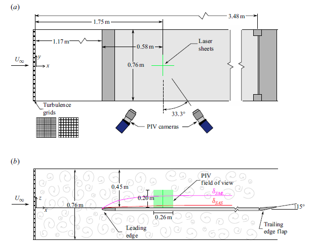
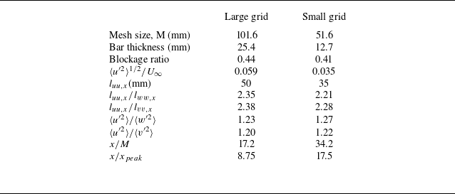
The experimental data examining the interaction of free-stream turbulence with an impermeable surface were collected in the University of Colorado Boulder (UCB) Low-Speed Unsteady Wind Tunnel facility. A schematic of the UCB experiment is presented in figure 2. This facility is an open-return wind tunnel with a test section that is 0.76 m wide, by 0.76 m tall and 3.58 m long. A detailed description of this facility and its capabilities is given in Farnsworth et al. (Reference Farnsworth, Sinner, Gloutak, Droste and Bateman2020). A flat-plate assembly was mounted within the wind tunnel test section, and tailored turbulence eddies were advected over the plate’s surface by passing the initially low-turbulence free-stream flow through a specifically designed passive, rectangular turbulence grid. Two different grids were used with different mesh scales which are documented in table 1. The grids were manufactured from 3.2 mm thick aluminium sheets with the precise pattern cut by water jet. The grids were positioned in a groove between the wind tunnel contraction and test section such that all four edges were clamped. The classical rectangular grid geometry was selected as it creates a well-understood eddy structure that has been extensively used in wind tunnel turbulence research for decades (Roach Reference Roach1987). As the size of the turbulence structures is directly dependent on the mesh geometry the two mesh sizes were intentionally chosen to create turbulence that had characteristic length scales that differed by approximately a factor of two. For each grid and PIV measurement configuration, a data set was collected without the flat plate installed to characterise the turbulence produced by each grid without alteration by the impermeable flat plate. The resulting turbulence parameters for both grids, measured using PIV at a consistent distance of $x = 1.75\,\rm m$
downstream from the grids and a free-stream velocity of
$x = 1.75\,\rm m$
downstream from the grids and a free-stream velocity of $15\,\rm ms^{-1}$
, are presented table 1. By decreasing the mesh size between the two grids, the streamwise turbulence intensity,
$15\,\rm ms^{-1}$
, are presented table 1. By decreasing the mesh size between the two grids, the streamwise turbulence intensity, $\langle u'^2\rangle ^{1/2}/U_\infty$
, and integral length scales both decrease, where
$\langle u'^2\rangle ^{1/2}/U_\infty$
, and integral length scales both decrease, where $u'$
is the fluctuating streamwise velocity component and
$u'$
is the fluctuating streamwise velocity component and $U_\infty$
is the mean free-stream velocity. Note that the ratios of velocity variances,
$U_\infty$
is the mean free-stream velocity. Note that the ratios of velocity variances, $\langle u'^2\rangle /\langle w'^2\rangle$
and
$\langle u'^2\rangle /\langle w'^2\rangle$
and $\langle u'^2\rangle /\langle v'^2\rangle$
, for the turbulence grids tested are between 1.2 and 1.3, indicating a deviation from isotropic turbulence in the test section; which is consistent with the prior characterisation of classical turbulence grids (Roach Reference Roach1987).
$\langle u'^2\rangle /\langle v'^2\rangle$
, for the turbulence grids tested are between 1.2 and 1.3, indicating a deviation from isotropic turbulence in the test section; which is consistent with the prior characterisation of classical turbulence grids (Roach Reference Roach1987).
Turbulence grid geometry and resulting free-stream turbulence characteristics measured $1.75$
m from the grids without the plate installed. Here,
$1.75$
m from the grids without the plate installed. Here, $x$
indicates the downstream location of the measurement from the grid and
$x$
indicates the downstream location of the measurement from the grid and $x_{peak}$
the location of maximum turbulence intensity behind the grid.
$x_{peak}$
the location of maximum turbulence intensity behind the grid.
The flat-plate assembly was installed in the test section $1.17\,\rm m$
downstream of the turbulence grids to provide sufficient downstream distance for the wakes created by the individual bars of the grids to fully develop and equilibrate before interacting with the flat plate. From prior hot-wire anemometry characterisation of the large grid in the UCB facility, the location of the peak turbulence intensity was found to be
$1.17\,\rm m$
downstream of the turbulence grids to provide sufficient downstream distance for the wakes created by the individual bars of the grids to fully develop and equilibrate before interacting with the flat plate. From prior hot-wire anemometry characterisation of the large grid in the UCB facility, the location of the peak turbulence intensity was found to be $x_{peak}=0.2\,\rm m$
, which aligns with the predicted value from the ‘wake interaction distance’ method developed by Mazellier & Vassilicos (Reference Mazellier and Vassilicos2010). Additionally, vertical hot-wire profiles of the large grid showed that the cross-tunnel variability of the mean velocity is less than 1 % at a distance
$x_{peak}=0.2\,\rm m$
, which aligns with the predicted value from the ‘wake interaction distance’ method developed by Mazellier & Vassilicos (Reference Mazellier and Vassilicos2010). Additionally, vertical hot-wire profiles of the large grid showed that the cross-tunnel variability of the mean velocity is less than 1 % at a distance $1$
m from the grids. Corresponding measurements of the small grid were not collected, but as the size of the mesh is smaller, the wake interaction distance is less than that of the large grid, and
$1$
m from the grids. Corresponding measurements of the small grid were not collected, but as the size of the mesh is smaller, the wake interaction distance is less than that of the large grid, and $x_{peak}$
is estimated to be 0.1 m from the method of Mazellier & Vassilicos (Reference Mazellier and Vassilicos2010). The plate leading edge was positioned downstream of the point where the large grid turbulence is considered fully homogeneous across the test section of the wind tunnel. The leading edge of the flat plate had a modified super-elliptical shape with an aspect ratio of eight and a geometric cross-sectional blockage of 4.75 %. An adjustable trailing edge flap was used to set the stagnation point at the leading edge, using a leading edge pressure port and a Scanivalve DSA 3217 pressure scanner. This ensured that the flow remained attached along the upper surface of the leading edge and minimised the streamwise pressure gradient along the length of the plate surface. The resulting trailing edge flap angle was
$x_{peak}$
is estimated to be 0.1 m from the method of Mazellier & Vassilicos (Reference Mazellier and Vassilicos2010). The plate leading edge was positioned downstream of the point where the large grid turbulence is considered fully homogeneous across the test section of the wind tunnel. The leading edge of the flat plate had a modified super-elliptical shape with an aspect ratio of eight and a geometric cross-sectional blockage of 4.75 %. An adjustable trailing edge flap was used to set the stagnation point at the leading edge, using a leading edge pressure port and a Scanivalve DSA 3217 pressure scanner. This ensured that the flow remained attached along the upper surface of the leading edge and minimised the streamwise pressure gradient along the length of the plate surface. The resulting trailing edge flap angle was $15^\circ$
for the specific configuration of this experiment. A complete description of the flat-plate assembly design can be found in Straccia (Reference Straccia2022).
$15^\circ$
for the specific configuration of this experiment. A complete description of the flat-plate assembly design can be found in Straccia (Reference Straccia2022).
A series of preliminary measurements were conducted at multiple streamwise locations along the plate and for a selection of free-stream velocities. From these measurements, a location of $x = 0.58$
m downstream of the plate leading edge was selected in order to (i) minimise the thickness of the near-wall viscous boundary layer or surface-adjacent sub-layer and (ii) provide the turbulence eddies sufficient fetch and advection time to be modified by the surface, creating a relatively thick SML. The cross-stream PIV field of view was located at this distance,
$x = 0.58$
m downstream of the plate leading edge was selected in order to (i) minimise the thickness of the near-wall viscous boundary layer or surface-adjacent sub-layer and (ii) provide the turbulence eddies sufficient fetch and advection time to be modified by the surface, creating a relatively thick SML. The cross-stream PIV field of view was located at this distance, $x = 0.58$
m downstream of the plate leading edge, and the streamwise PIV field of view was centred at this distance. A single free-stream velocity of
$x = 0.58$
m downstream of the plate leading edge, and the streamwise PIV field of view was centred at this distance. A single free-stream velocity of $15\,\mathrm {m\,s^{-1}}$
was also selected to reduce, as much as possible, the thickness of the wall-adjacent viscous boundary layer or surface-adjacent sub-layer.
$15\,\mathrm {m\,s^{-1}}$
was also selected to reduce, as much as possible, the thickness of the wall-adjacent viscous boundary layer or surface-adjacent sub-layer.
Stereoscopic PIV measurements were collected for two different measurement configurations within the UCB facility, namely: (i) a cross-stream $y{-}z$
plane and (ii) a streamwise
$y{-}z$
plane and (ii) a streamwise $x{-}z$
plane, as shown in figure 2. Two
$x{-}z$
plane, as shown in figure 2. Two $2560 \times 2160$
pixel 16-bit dynamic range sCMOS cameras equipped with 50 mm Nikkor lenses, anti-peak locking filters and Scheimpflug adapters were positioned in a stereoscopic configuration with a separation angle of
$2560 \times 2160$
pixel 16-bit dynamic range sCMOS cameras equipped with 50 mm Nikkor lenses, anti-peak locking filters and Scheimpflug adapters were positioned in a stereoscopic configuration with a separation angle of $67^\circ$
between them on one side of the wind tunnel. Illumination was provided by a Quantel Evergreen 200 dual-pulsed 532 nm Nd:YAG laser which was expanded into a sheet with a cylindrical lens with a focal length of −10 mm before entering the tunnel through the test-section ceiling. To transition from the streamwise to cross-stream stereoscopic PIV data collection orientation, the laser sheet was rotated
$67^\circ$
between them on one side of the wind tunnel. Illumination was provided by a Quantel Evergreen 200 dual-pulsed 532 nm Nd:YAG laser which was expanded into a sheet with a cylindrical lens with a focal length of −10 mm before entering the tunnel through the test-section ceiling. To transition from the streamwise to cross-stream stereoscopic PIV data collection orientation, the laser sheet was rotated $90^\circ$
and thickened from 1 to 2 mm. The wind tunnel was seeded with di-ethyl-hexyl-sebacic-acid-ester aerosol particles with a mean diameter of the order of
$90^\circ$
and thickened from 1 to 2 mm. The wind tunnel was seeded with di-ethyl-hexyl-sebacic-acid-ester aerosol particles with a mean diameter of the order of $1\, {\unicode{x03BC}}$
m using a LaVision aerosol generator. The field of view of the stereoscopic PIV measurement planes was large enough to resolve multiple free-stream turbulence structures while also capturing the top edge of the viscous boundary layer, adjacent to the plate surface as depicted in the schematic in figure 2. Note that the camera field of view does not include the inner region of the TBL, or surface-adjacent sub-layer, since this is not the focus of the current study. Table 2 presents the detailed stereoscopic PIV measurement parameters for each of the two configurations.
$1\, {\unicode{x03BC}}$
m using a LaVision aerosol generator. The field of view of the stereoscopic PIV measurement planes was large enough to resolve multiple free-stream turbulence structures while also capturing the top edge of the viscous boundary layer, adjacent to the plate surface as depicted in the schematic in figure 2. Note that the camera field of view does not include the inner region of the TBL, or surface-adjacent sub-layer, since this is not the focus of the current study. Table 2 presents the detailed stereoscopic PIV measurement parameters for each of the two configurations.
PIV parameters for grid-turbulence experiment at UCB and TBL experiment at LMFL.

The stereoscopic PIV images were recorded with the LaVision DaVis 10 software package with the timing between the hardware managed using an internal LaVision PTU programmable timing unit. Thirty ensemble sets were collected for each measurement case at a frequency of 10 Hz over periods of 100 s. At this low sampling frequency the samples within an ensemble set are not time resolved and are considered independent. This sample size was determined from the preliminary measurement campaigns to be a sufficient sample size to provide converged turbulence statistics, most notably for the integral length scale calculations. Vector fields were calculated in DaVis 10 using a multipass processing method with four passes and a 50 % interrogation window overlap starting at an interrogation window size of $96 \times 96$
pixels, and decreasing to a final interrogation window size of
$96 \times 96$
pixels, and decreasing to a final interrogation window size of $24 \times 24$
pixels with a Gaussian weighting function applied on the final pass. This provided a final velocity vector resolution of 0.833 vectors/mm in both directions and for both data collection orientations. The measurement uncertainties in the three velocity components,
$24 \times 24$
pixels with a Gaussian weighting function applied on the final pass. This provided a final velocity vector resolution of 0.833 vectors/mm in both directions and for both data collection orientations. The measurement uncertainties in the three velocity components, $\sigma _u$
,
$\sigma _u$
, $\sigma _v$
and
$\sigma _v$
and $\sigma _w$
, were calculated using the correlation statistics method in DaVis 10 (details are given in Wieneke Reference Wieneke2015). The root mean square of the uncertainty normalised by the mean streamwise velocity magnitude is calculated across frames and spatial dimensions to summarise the quantity and presented in table 2 as
$\sigma _w$
, were calculated using the correlation statistics method in DaVis 10 (details are given in Wieneke Reference Wieneke2015). The root mean square of the uncertainty normalised by the mean streamwise velocity magnitude is calculated across frames and spatial dimensions to summarise the quantity and presented in table 2 as $(\sigma _u/U)^{rms}$
. The uncertainty in all three velocity components is below 1 % of the mean free-stream velocity for the streamwise configuration, while uncertainty in the cross-stream plane is as high as 1.5 % for the out-of-plane component.
$(\sigma _u/U)^{rms}$
. The uncertainty in all three velocity components is below 1 % of the mean free-stream velocity for the streamwise configuration, while uncertainty in the cross-stream plane is as high as 1.5 % for the out-of-plane component.
2.2. Shear-dominated surface layer: turbulent boundary layer case (LMFL facility)
The experimental data sets applied to the analysis of the surface layer within the canonical flat-plate TBL were collected within the High Reynolds Number Turbulent Boundary Layer Wind Tunnel Facility at the Laboratoire de Mécanique des Fluides de Lille (LMFL). This facility is a closed return wind tunnel with a test section that is 2 m wide, 1 m tall and 20.6 m long. A single set of flow conditions was explored for the canonical TBL, namely: a nominal inlet velocity of $3\,\mathrm {m\,s^{-1}}$
with free-stream velocity of
$3\,\mathrm {m\,s^{-1}}$
with free-stream velocity of $3.36\,\mathrm {m\,s^{-1}}$
at the measurement location which was
$3.36\,\mathrm {m\,s^{-1}}$
at the measurement location which was $19.35\,\mathrm {m}$
downstream from the entrance to the wind tunnel test section. This location was selected to maximise the boundary layer thickness. The Reynolds number of the resulting boundary layer was
$19.35\,\mathrm {m}$
downstream from the entrance to the wind tunnel test section. This location was selected to maximise the boundary layer thickness. The Reynolds number of the resulting boundary layer was $Re_\theta = 7680\,(Re_\tau =2260)$
with a boundary layer thickness of
$Re_\theta = 7680\,(Re_\tau =2260)$
with a boundary layer thickness of $\delta _{99}=0.278$
m; additional parameters for the TBL are given in table 3. To calculate the viscous length scale,
$\delta _{99}=0.278$
m; additional parameters for the TBL are given in table 3. To calculate the viscous length scale, $\delta _\nu$
, and the wall units (e.g.
$\delta _\nu$
, and the wall units (e.g. $z^+$
), the friction velocity was approximated by comparing these data with a prior detailed characterisation of the boundary layer facility which resolved the near-wall viscous sub-layer at similar operating conditions, as documented by Foucaut et al. (2018). In this prior study, the friction velocity,
$z^+$
), the friction velocity was approximated by comparing these data with a prior detailed characterisation of the boundary layer facility which resolved the near-wall viscous sub-layer at similar operating conditions, as documented by Foucaut et al. (2018). In this prior study, the friction velocity, $u_\tau ,$
was determined by fitting the linear region of the mean velocity profile within the viscous sub-layer using highly resolved near-wall planar PIV measurements. By comparing the mean velocity profiles of the current data and the reference data set the friction velocity can be adjusted to match the mean velocity profiles where there is overlap. With this method we find that the friction velocity that collapses the current data set to the reference data set is only 0.7 % greater than that of the reference case.
$u_\tau ,$
was determined by fitting the linear region of the mean velocity profile within the viscous sub-layer using highly resolved near-wall planar PIV measurements. By comparing the mean velocity profiles of the current data and the reference data set the friction velocity can be adjusted to match the mean velocity profiles where there is overlap. With this method we find that the friction velocity that collapses the current data set to the reference data set is only 0.7 % greater than that of the reference case.
The canonical TBL parameters from the LMFL experiment; free-stream velocity, $U_\infty$
, momentum thickness Reynolds number,
$U_\infty$
, momentum thickness Reynolds number, $Re_\theta$
, friction Reynolds number,
$Re_\theta$
, friction Reynolds number, $Re_\tau$
, boundary layer thickness,
$Re_\tau$
, boundary layer thickness, $\delta _{99}$
, momentum thickness,
$\delta _{99}$
, momentum thickness, $\theta$
, displacement thickness,
$\theta$
, displacement thickness, $\delta ^*$
, and viscous length scale,
$\delta ^*$
, and viscous length scale, $\delta _\nu$
.
$\delta _\nu$
.

The turbulence generated within the TBL is strongly anisotropic, whereas the turbulence generated by the grids is approximately isotropic prior to interactions with the flat plate. Furthermore, the turbulence within the TBL is strongly influenced by shear and production which are both absent in the grid-turbulence experiment external to the surface-adjacent sub-layer. To compare the relative strength of the turbulence across these experiments, the turbulent Reynolds numbers based on the streamwise and surface-normal velocity fluctuations, $\langle u'^2\rangle ^{1/2}$
and
$\langle u'^2\rangle ^{1/2}$
and $\langle w'^2\rangle ^{1/2}$
, and the streamwise turbulence length scales of these velocity components,
$\langle w'^2\rangle ^{1/2}$
, and the streamwise turbulence length scales of these velocity components, $l_{uu,x}$
and
$l_{uu,x}$
and $l_{ww,x}$
, are defined by
$l_{ww,x}$
, are defined by
 \begin{equation} Re_{l_u} = \frac {\left\langle u'^2\right\rangle ^{1/2} l_{uu,x}}{\nu }, \end{equation}
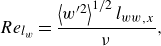 \begin{equation} Re_{l_w} = \frac {\left\langle w'^2\right\rangle ^{1/2} l_{ww,x}}{\nu }, \end{equation}
and are presented for reference in table 4. In the grid-turbulence experiment, the Reynolds number velocity and length scales are defined in the free stream while for the TBL the Reynolds numbers are defined at the upper bound of the surface-layer region, $\delta _U$
, as defined in § 3. From table 4 it can be observed that the Reynolds number based upon the surface-normal velocity component,
$\delta _U$
, as defined in § 3. From table 4 it can be observed that the Reynolds number based upon the surface-normal velocity component, $Re_{l_w}$
, for the TBL is much less than that of the grid-turbulence cases, whereas the Reynolds number based upon the streamwise velocity component,
$Re_{l_w}$
, for the TBL is much less than that of the grid-turbulence cases, whereas the Reynolds number based upon the streamwise velocity component, $Re_{l_u}$
, is between that of the two grid-turbulence cases.
$Re_{l_u}$
, is between that of the two grid-turbulence cases.


Schematic of LMFL TBL wind tunnel experiment and stereoscopic PIV measurement system depicting both the streamwise and cross-stream measurement configurations.

Three-component velocity fields were measured for two-dimensional planes using high-speed stereoscopic PIV. Three different measurement configurations were used: (i) a cross-stream $y{-}z$
plane, (ii) a streamwise
$y{-}z$
plane, (ii) a streamwise $x{-}z$
plane and (iii) an expanded field-of-view streamwise
$x{-}z$
plane and (iii) an expanded field-of-view streamwise $x{-}z$
plane. A schematic of this experimental set-up is presented in figure 3. Two Phantom Miro M340 cameras, equipped with 60 mm Micro Nikkor lenses and Scheimpflug lens adapters, were positioned beneath the glass floor of the wind tunnel looking obliquely upwards at the floor (as depicted in figure 3). Illumination was provided by a Quantronix Darwin Duo laser which was expanded into a sheet with a cylindrical lens with a focal length of −60 mm or −80 mm, for configuration 1 or configurations 2 and 3, respectively, before entering the tunnel through the ceiling. To transition from the cross-stream to the streamwise orientation, the cameras and laser sheet were rotated horizontally by
$x{-}z$
plane. A schematic of this experimental set-up is presented in figure 3. Two Phantom Miro M340 cameras, equipped with 60 mm Micro Nikkor lenses and Scheimpflug lens adapters, were positioned beneath the glass floor of the wind tunnel looking obliquely upwards at the floor (as depicted in figure 3). Illumination was provided by a Quantronix Darwin Duo laser which was expanded into a sheet with a cylindrical lens with a focal length of −60 mm or −80 mm, for configuration 1 or configurations 2 and 3, respectively, before entering the tunnel through the ceiling. To transition from the cross-stream to the streamwise orientation, the cameras and laser sheet were rotated horizontally by $90^\circ$
. The width of the laser sheet was approximately 1.2 mm at its waist. For the data taken in the cross-stream
$90^\circ$
. The width of the laser sheet was approximately 1.2 mm at its waist. For the data taken in the cross-stream $y{-}z$
plane, the two laser pulses were offset from one another in the streamwise direction to increase the cross-stream particle displacements and maximise the number of consistent particles illuminated in the time-separated fields of view for both pulses. The streamwise offset was 0.48 mm between the first and second laser pulses, resulting in an estimated 68 % retention of the particles between the two frames. The flow was seeded with poly-ethylene glycol particles within the return leg of the wind tunnel resulting in particle sizes of the order of
$y{-}z$
plane, the two laser pulses were offset from one another in the streamwise direction to increase the cross-stream particle displacements and maximise the number of consistent particles illuminated in the time-separated fields of view for both pulses. The streamwise offset was 0.48 mm between the first and second laser pulses, resulting in an estimated 68 % retention of the particles between the two frames. The flow was seeded with poly-ethylene glycol particles within the return leg of the wind tunnel resulting in particle sizes of the order of $1\, {\unicode{x03BC}}$
m in diameter. The two primary configurations, (i) the cross-stream
$1\, {\unicode{x03BC}}$
m in diameter. The two primary configurations, (i) the cross-stream $y{-}z$
and (ii) streamwise
$y{-}z$
and (ii) streamwise $x{-}z$
planes, had a wall-normal field of view that captured approximately
$x{-}z$
planes, had a wall-normal field of view that captured approximately $0.3\delta _{99}$
to maximise the vector resolution in the near-wall inertial surface-layer region. The third configuration, (iii) the streamwise expanded
$0.3\delta _{99}$
to maximise the vector resolution in the near-wall inertial surface-layer region. The third configuration, (iii) the streamwise expanded $x{-}z$
plane, extended to approximately
$x{-}z$
plane, extended to approximately $1.25\delta _{99}$
to measure the total boundary layer thickness and free-stream velocity. Table 2 presents the PIV parameters for each of the three configurations.
$1.25\delta _{99}$
to measure the total boundary layer thickness and free-stream velocity. Table 2 presents the PIV parameters for each of the three configurations.
The stereoscopic PIV image sets were recorded with the LaVision DaVis 10 software package and the timing between the hardware was managed using an external LaVision PTU-X programmable timing unit. At the high sampling rate of configurations (i) and (ii) the data are considered time resolved or correlated between snapshots. Because of this, a larger number of ensemble sets were required to achieve similar statistical convergence to the grid-turbulence experiments. The time resolution of the LMFL data is used for calculation of two-point correlations in the streamwise direction, as will be discussed in the next subsection, but is not used for analysis of structures through time in the present work. Therefore, the difference in sampling frequency between the UCB and LMFL data sets does not impact the analysis of the turbulence statistical structure. Vector fields were calculated within MATLAB using a multipass cross-correlation method adapted from MATLAB’s matpiv library. The processing consisted of four passes each using a 64 % average interrogation window overlap where the interrogation window started with a size of $64 \times 64$
pixels and was decreased to
$64 \times 64$
pixels and was decreased to $22 \times 16$
pixels for the final pass. This provided a velocity vector resolution of 1.54 vectors/mm in both directions for configurations (i) and (ii), and 1.33 vectors/mm in both directions for configuration (iii). The measurement uncertainty was calculated from the final vector fields by calculating the root mean square difference between adjacent vectors, which is the method for calculating random error in Adrian & Westerweel (Reference Adrian and Westerweel2011). This method is effectively the same as that implemented in Herpin et al. (2008), but uses adjacent vectors rather than overlapping PIV systems. The uncertainty calculated with this approach was found to agree with that calculated for a single set of 3231 images using the correlation statistics method in the DaVis software used with the UCB data (Wieneke Reference Wieneke2015).
$22 \times 16$
pixels for the final pass. This provided a velocity vector resolution of 1.54 vectors/mm in both directions for configurations (i) and (ii), and 1.33 vectors/mm in both directions for configuration (iii). The measurement uncertainty was calculated from the final vector fields by calculating the root mean square difference between adjacent vectors, which is the method for calculating random error in Adrian & Westerweel (Reference Adrian and Westerweel2011). This method is effectively the same as that implemented in Herpin et al. (2008), but uses adjacent vectors rather than overlapping PIV systems. The uncertainty calculated with this approach was found to agree with that calculated for a single set of 3231 images using the correlation statistics method in the DaVis software used with the UCB data (Wieneke Reference Wieneke2015).
2.3. Estimation of integral length scales
A central aspect of our work is to examine how integral length scales vary with distance from the surface. The process for calculating the integral length scale has been refined to minimise the experimental variability in the results while also providing a consistent method for each component direction. Note that the integral length scale is a correlation length that characterises the inertial energy-containing motions within the turbulent velocity field. The quantification of the integral scale for a particular pair of velocity fluctuations in a specified direction requires integrating the two-point correlation coefficient from zero to infinity. For a three component flow field $u_\alpha$
(
$u_\alpha$
( $\alpha =1,2,3$
) in three-dimensional space measured with Cartesian coordinates
$\alpha =1,2,3$
) in three-dimensional space measured with Cartesian coordinates $x_\beta$
(
$x_\beta$
( $\beta = 1,2,3$
), nine integral length scales can be defined. To account for non-homogeneity in the wall-normal direction, we apply the following form of the two-point the correlation coefficient:
$\beta = 1,2,3$
), nine integral length scales can be defined. To account for non-homogeneity in the wall-normal direction, we apply the following form of the two-point the correlation coefficient:
 \begin{equation} R_{u_\alpha u_\alpha ,x_\beta }\left (\mathbf {x}, r_{x_\beta }\right ) = \frac {\left\langle u_\alpha '\left (\mathbf {x}\right )u_\alpha '\left (\mathbf {x}+r_{x_\beta }\hat {e}_{x_\beta }\right )\right\rangle }{\left\langle u_\alpha '^2\left (\mathbf {x}\right )\right\rangle ^{1/2} \left\langle u_\alpha '^2\left (\mathbf {x}+r_{x_\beta }\hat {e}_{x_\beta }\right )\right\rangle ^{1/2}}. \end{equation}
This method for normalisation has been implemented previously by Ganapathisubramani et al. (Reference Ganapathisubramani, Hutchins, Hambleton, Longmire and Marusic2005) and Christensen & Adrian (Reference Christensen and Adrian2001), and is used in this work for the calculation of all correlation coefficients. Whereas local normalisation of fluctuating velocity in the inhomogeneous wall-normal direction is particularly important, we also account for small levels of inhomogeneity in the streamwise direction in both the grid turbulence and TBL analyses.
Ideally, the normalised correlation coefficient would be integrated with respect to $r_{x_\beta }$
to infinity or the first zero crossing if oscillatory. A difficulty with PIV data is that the spatial range of the correlation is limited by the limited field of view of the measurement domain. Additionally, significant variability in the tails of the correlation curve is encountered as the correlation curve approaches zero due to the measurement noise in the PIV system. This variability induces considerable variation in the zero-crossing point of the correlation curves. To minimise these issues, the limit of the integral is defined to be the distance where the normalised correlation reaches a consistently specified
$r_{x_\beta }$
to infinity or the first zero crossing if oscillatory. A difficulty with PIV data is that the spatial range of the correlation is limited by the limited field of view of the measurement domain. Additionally, significant variability in the tails of the correlation curve is encountered as the correlation curve approaches zero due to the measurement noise in the PIV system. This variability induces considerable variation in the zero-crossing point of the correlation curves. To minimise these issues, the limit of the integral is defined to be the distance where the normalised correlation reaches a consistently specified $R_{cut}$
value close to, but above, zero as defined by
$R_{cut}$
value close to, but above, zero as defined by
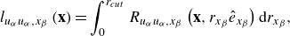 \begin{equation} l_{u_\alpha u_\alpha ,x_\beta }\left (\mathbf {x}\right ) = \int _0^{r_{cut}}R_{u_\alpha u_\alpha ,x_\beta }\left (\mathbf {x}, r_{x_\beta }\hat {e}_{x_\beta }\right ){\rm d}r_{x_\beta } ,\end{equation}
where $r_{cut}$
is the correlation distance at which the correlation function crosses the cutoff value
$r_{cut}$
is the correlation distance at which the correlation function crosses the cutoff value $R_{cut} = 0.03$
. The value of
$R_{cut} = 0.03$
. The value of $R_{cut} = 0.03$
was selected to minimise the amount of the correlation curve discarded while staying above the point where there is considerable noise in the correlation curve. Assuming an exponential form of the correlation curve the threshold value of
$R_{cut} = 0.03$
was selected to minimise the amount of the correlation curve discarded while staying above the point where there is considerable noise in the correlation curve. Assuming an exponential form of the correlation curve the threshold value of $R_{cut} = 0.03$
will systematically under calculate the integral length scale by 3 %, but preserves the underlying trends in the integral length scales while avoiding noise in the calculation due to variability in the tails near zero. Further details on the integral length scale calculation are provided in Appendix A.
$R_{cut} = 0.03$
will systematically under calculate the integral length scale by 3 %, but preserves the underlying trends in the integral length scales while avoiding noise in the calculation due to variability in the tails near zero. Further details on the integral length scale calculation are provided in Appendix A.
For the SDSL data within the TBL, the streamwise extent of the spatial field of view was not sufficient to calculate the tails of the correlation curve. For these length scales the correlation was calculated in time and then converted to space using a classical application of Taylor’s frozen turbulence hypothesis with the local mean velocity used as the convective velocity as defined by
 \begin{equation} R_{u_\alpha u_\alpha ,x}\left (\mathbf {x}, [\delta {t}*U]\hat {e}_{x}\right ) = R_{u_\alpha u_\alpha ,t}\left (\mathbf {x}, \delta {t}\right ). \end{equation}
Taylor’s hypothesis has been widely applied in TBLs with hot-wire measurements and the applicability has been extensively explored. Geng et al. (Reference Geng, He, Wang, Xu, Lozano-Durán and Wallace2015) determined that the appropriate convective velocity above $z+$
of 20 is the mean velocity, while Dennis & Nickels (Reference Dennis and Nickels2008) demonstrated the accuracy of Taylor’s hypothesis in reconstructing large structures over distances of up to
$z+$
of 20 is the mean velocity, while Dennis & Nickels (Reference Dennis and Nickels2008) demonstrated the accuracy of Taylor’s hypothesis in reconstructing large structures over distances of up to $6\delta$
. The correlation curves calculated using the temporal resolution were directly compared with the portion of the correlation curve that could be calculated from the spatial resolution to validate this approach. The two methods were found to align very well across the extent of the correlation available, therefore it was determined that this approach could accurately quantify the spatial correlation and was assumed to be more accurate than fitting an exponential curve to the data for extrapolating the tail of the correlation curve.
$6\delta$
. The correlation curves calculated using the temporal resolution were directly compared with the portion of the correlation curve that could be calculated from the spatial resolution to validate this approach. The two methods were found to align very well across the extent of the correlation available, therefore it was determined that this approach could accurately quantify the spatial correlation and was assumed to be more accurate than fitting an exponential curve to the data for extrapolating the tail of the correlation curve.
3. The surface layers
As discussed in § 1 and illustrated in figure 1(a), a primary aim of this study is to establish the existence of a surface layer in the two experimentally generated flows described in § 2, where the ‘surface layer’ is defined as an inertia-dominated near-surface region outside a SAS with linear growth in one or more integral scales. In this section the variations with $z$
of different integral scales are quantified to determine which, if any, scale on
$z$
of different integral scales are quantified to determine which, if any, scale on $z$
versus those that do not, above a SAS. Of particular interest are the differences and similarities between canonical shear-dominated and non-canonical shear-free surface layers.
$z$
versus those that do not, above a SAS. Of particular interest are the differences and similarities between canonical shear-dominated and non-canonical shear-free surface layers.
3.1. The existence of the shear-free surface layer
Wall-normal profile of the horizontal integral length scales of vertical velocity fluctuations in the streamwise direction ( $l_{ww,x}(z)$
) for (a) the large grid and (b) the small grid. Using similar notation as in figure 1, the green dashed lines define the upper (
$l_{ww,x}(z)$
) for (a) the large grid and (b) the small grid. Using similar notation as in figure 1, the green dashed lines define the upper ( $\delta _U$
) and lower (
$\delta _U$
) and lower ( $\delta _L$
) margins of the linear region, the magenta dashed line is the upper margin of the SML (
$\delta _L$
) margins of the linear region, the magenta dashed line is the upper margin of the SML ( $\delta _{SML}$
) and the red dashed line is the upper margin of the SAS (
$\delta _{SML}$
) and the red dashed line is the upper margin of the SAS ( $\delta _{SAS}$
) estimated as
$\delta _{SAS}$
) estimated as $\delta _{99}$
.
$\delta _{99}$
.

Wall-normal profiles of integral length scales of (a,c) streamwise velocity fluctuations in the streamwise direction ( $l_{uu,x}(z)$
) and (b,d) cross-stream velocity fluctuations in the streamwise direction (
$l_{uu,x}(z)$
) and (b,d) cross-stream velocity fluctuations in the streamwise direction ( $l_{vv,x}(z)$
). The top row (a,b) is for the large grid and the bottom (c,d) for the small. Using similar notation as in figure 4, the green dashed lines define the upper (
$l_{vv,x}(z)$
). The top row (a,b) is for the large grid and the bottom (c,d) for the small. Using similar notation as in figure 4, the green dashed lines define the upper ( $\delta _U$
) and lower (
$\delta _U$
) and lower ( $\delta _L$
) margins of the linear region, the magenta dashed line is the upper margin of the SML (
$\delta _L$
) margins of the linear region, the magenta dashed line is the upper margin of the SML ( $\delta _{SML}$
) and the red dashed line is the upper margin of the SAS (
$\delta _{SML}$
) and the red dashed line is the upper margin of the SAS ( $\delta _{SAS}$
) estimated using
$\delta _{SAS}$
) estimated using $\delta _{99}$
.
$\delta _{99}$
.

In figure 4, $l_{ww,x}$
is plotted against the distance from the plate,
$l_{ww,x}$
is plotted against the distance from the plate, $z$
, for the grid-turbulence experiments with both grids, where integral scales are quantified according to § 2.3. In this figure the black solid line is
$z$
, for the grid-turbulence experiments with both grids, where integral scales are quantified according to § 2.3. In this figure the black solid line is $l_{ww,x}(z)$
with the plate installed in the test section and the dotted line is without the plate. The SML is the region within the grid-generated turbulence where the integral length scale,
$l_{ww,x}(z)$
with the plate installed in the test section and the dotted line is without the plate. The SML is the region within the grid-generated turbulence where the integral length scale, $l_{ww,x}$
, is significantly modified by the interactions between the grid turbulence and the flat plate. Therefore,
$l_{ww,x}$
, is significantly modified by the interactions between the grid turbulence and the flat plate. Therefore, $\delta _{SML}$
is defined as the height below which
$\delta _{SML}$
is defined as the height below which $l_{ww,x}$
differs significantly from
$l_{ww,x}$
differs significantly from $l_{ww,x}$
at the measurement location without the plate installed, where ‘significantly’ is defined as within one standard deviation of the variation of
$l_{ww,x}$
at the measurement location without the plate installed, where ‘significantly’ is defined as within one standard deviation of the variation of $l_{ww,x}(z)$
over the test section without the plate. The value of
$l_{ww,x}(z)$
over the test section without the plate. The value of $\delta _{SML}$
is shown with the magenta dashed line in figure 4. As will be discussed below, two internal layers within the SML are objectively quantified: (i) the SAS (red dashed line), and (ii) the inertial SFSL (green dashed lines).
$\delta _{SML}$
is shown with the magenta dashed line in figure 4. As will be discussed below, two internal layers within the SML are objectively quantified: (i) the SAS (red dashed line), and (ii) the inertial SFSL (green dashed lines).
The SAS was discussed in § 1 in context with figure 1(b). It forms as the grid turbulence embedded within a quasi-uniform mean flow passes over the flat plate, creating a sub-layer adjacent to the surface with a mix of highly non-steady frictional stresses and turbulence production very close to the surface from the distortion of turbulence by a high mean shear rate. The surface-adjacent shear-generated turbulence and strong frictional stresses fill a region akin to a highly non-canonical TBL. We define the thickness of this SAS as the height at which the mean velocity profile is $99\%$
of the free-stream value,
$99\%$
of the free-stream value, $U(\delta _{SAS}) = 0.99U_\infty$
, where
$U(\delta _{SAS}) = 0.99U_\infty$
, where $U_\infty$
is the mean velocity in the free stream (outside the surface-modified region). The SAS region, indicated by a dashed horizontal red line in figure 4, is discussed in more detail in § 4.
$U_\infty$
is the mean velocity in the free stream (outside the surface-modified region). The SAS region, indicated by a dashed horizontal red line in figure 4, is discussed in more detail in § 4.
In figure 5 we plot the streamwise integral scales of the two horizontal components of fluctuating velocity over $z$
for the two grids. From figures 4 and 5 it is apparent that only the vertical velocity generates a horizontal integral scale that clearly increases with distance from the surface through the inertia-dominated region above, and separated from, the SAS (the red-dashed line). The SFSL is therefore defined from the regions of clear linear increase in
$z$
for the two grids. From figures 4 and 5 it is apparent that only the vertical velocity generates a horizontal integral scale that clearly increases with distance from the surface through the inertia-dominated region above, and separated from, the SAS (the red-dashed line). The SFSL is therefore defined from the regions of clear linear increase in $l_{ww,x}$
with
$l_{ww,x}$
with $z$
in figure 4 for both grids. The upper and lower margins of the linear regions are objectively defined as described in Appendix B using an iterative procedure to identify the portion of the curve that is ‘most’ linear. This approach limits bias in quantifying
$z$
in figure 4 for both grids. The upper and lower margins of the linear regions are objectively defined as described in Appendix B using an iterative procedure to identify the portion of the curve that is ‘most’ linear. This approach limits bias in quantifying $\delta _U$
and
$\delta _U$
and $\delta _L$
, the upper and lower margins of the SFSL shown with green horizontal dashed lines. The coefficient of determination of the linear fit over the SFSL is 0.997 and 0.992 for the large and small grids, respectively. As will be discussed in § 4, the mean shear rate is zero within and above this ‘shear-free’ surface-layer region.
$\delta _L$
, the upper and lower margins of the SFSL shown with green horizontal dashed lines. The coefficient of determination of the linear fit over the SFSL is 0.997 and 0.992 for the large and small grids, respectively. As will be discussed in § 4, the mean shear rate is zero within and above this ‘shear-free’ surface-layer region.
Normalised thicknesses of the SAS, SFSL and SML for both grid cases are given in table 5. The upper boundary of the surface-modified region for the small and large grids is found to extend to approximately two free-stream streamwise integral length scales, $l_{uu,x\infty }$
, from the surface:
$l_{uu,x\infty }$
, from the surface: $\delta _{SML}\approx 2l_{uu,x\infty }$
. Because the longitudinal integral length scale quantifies the coherence length of the energy-dominant eddies in the quasi-isotropic free-stream turbulence, it is not surprising that the thickness of the SML scales on the coherence length of the energy-containing turbulence motions that interact with the surface. This result is consistent with TH77, who measured the influence of the surface to extend to roughly twice the free-stream streamwise integral scale in their moving wall experiment, as well as with the theoretical predictions of HG78, where we use the acronyms HG78 for Hunt & Graham (Reference Hunt and Graham1978) and TH77 for Thomas & Hancock (Reference Thomas and Hancock1977).
$\delta _{SML}\approx 2l_{uu,x\infty }$
. Because the longitudinal integral length scale quantifies the coherence length of the energy-dominant eddies in the quasi-isotropic free-stream turbulence, it is not surprising that the thickness of the SML scales on the coherence length of the energy-containing turbulence motions that interact with the surface. This result is consistent with TH77, who measured the influence of the surface to extend to roughly twice the free-stream streamwise integral scale in their moving wall experiment, as well as with the theoretical predictions of HG78, where we use the acronyms HG78 for Hunt & Graham (Reference Hunt and Graham1978) and TH77 for Thomas & Hancock (Reference Thomas and Hancock1977).
Surface-layer parameters for the grid-turbulence SDSL and TBL SDSL.

The consistencies with the HG78 theory and TH77 experiments are particularly significant because these were developed with a moving wall to minimise the thickness of the SAS. Specifically, the theory was developed in the limit $\delta _{visc}/l_{uu,x\infty }\lt \lt 1$
, while TH77 estimated this ratio to be approximately 0.05 in their experiments, with
$\delta _{visc}/l_{uu,x\infty }\lt \lt 1$
, while TH77 estimated this ratio to be approximately 0.05 in their experiments, with $\delta _{visc}$
defined as a viscous scale in a laminar SAS. As shown in table 5, in our fixed-wall grid-turbulence experiments
$\delta _{visc}$
defined as a viscous scale in a laminar SAS. As shown in table 5, in our fixed-wall grid-turbulence experiments $\delta _{SAS}/\delta _{SML}\approx 0.15$
, where
$\delta _{SAS}/\delta _{SML}\approx 0.15$
, where $\delta _{SML}\approx 2l_{uu,x\infty }$
and
$\delta _{SML}\approx 2l_{uu,x\infty }$
and $\delta _{SAS}$
is defined as
$\delta _{SAS}$
is defined as $\delta _{99}$
, much thicker than the wall-adjacent viscous layer. Given the well-defined structure of the surface layers in figure 4, we conclude that the SASs in our fixed-wall experiments are sufficiently thin to maintain the nature of the turbulence-surface interactions that were modelled in the HG78 theory and measured in the TH77 experiments.
$\delta _{99}$
, much thicker than the wall-adjacent viscous layer. Given the well-defined structure of the surface layers in figure 4, we conclude that the SASs in our fixed-wall experiments are sufficiently thin to maintain the nature of the turbulence-surface interactions that were modelled in the HG78 theory and measured in the TH77 experiments.
Interestingly, the upper margin of the surface layer is approximately one free-stream streamwise integral length scale from the surface ( $\delta _U \approx l_{uu,x\infty }$
), and the thickness of the SFSL,
$\delta _U \approx l_{uu,x\infty }$
), and the thickness of the SFSL, $\Delta _{SL}=\delta _U-\delta _L$
, is approximately two thirds of the longitudinal integral scale in the free stream. These results are consistent between the two grids which create free-stream correlation lengths a factor of two different. As shown in figure 4, there exists a gap between the lower margin of the surface layer defined by linear growth in
$\Delta _{SL}=\delta _U-\delta _L$
, is approximately two thirds of the longitudinal integral scale in the free stream. These results are consistent between the two grids which create free-stream correlation lengths a factor of two different. As shown in figure 4, there exists a gap between the lower margin of the surface layer defined by linear growth in $l_{ww,x}$
, and the upper margin of the SAS as defined by
$l_{ww,x}$
, and the upper margin of the SAS as defined by $\delta _{99}$
. If the mechanism that creates linear growth in the integral length scale with
$\delta _{99}$
. If the mechanism that creates linear growth in the integral length scale with $z$
is associated with blockage at the impermeable plate and the inertia dominance of the free-stream eddies that are modified, the linear SFSL region will not initiate until some distance above the SAS where length scales associated with frictional stresses and turbulence production dominate. Table 5 indicates that the gap between
$z$
is associated with blockage at the impermeable plate and the inertia dominance of the free-stream eddies that are modified, the linear SFSL region will not initiate until some distance above the SAS where length scales associated with frictional stresses and turbulence production dominate. Table 5 indicates that the gap between $\delta _{SAS}$
and
$\delta _{SAS}$
and $\delta _L$
is approximately 30
$\delta _L$
is approximately 30 $\%$
of
$\%$
of $\delta _L$
. This transition will be further discussed in § 4.
$\delta _L$
. This transition will be further discussed in § 4.
The streamwise integral length scales of the horizontal velocity components $l_{uu,x}$
and
$l_{uu,x}$
and $l_{vv,x}$
plotted in figure 5 show consistency between the large and small grids. Importantly, none of these profiles increase with distance from the surface in the surface layer, much less linearly as is the case for
$l_{vv,x}$
plotted in figure 5 show consistency between the large and small grids. Importantly, none of these profiles increase with distance from the surface in the surface layer, much less linearly as is the case for $l_{ww,x}(z)$
. This significant result supports the hypothesis that the ‘special’ integral scales that display linear scaling with distance from the surface are those associated with vertical fluctuating velocity which feels directly the impacts of blockage at the impermeable surface. Contrasting figures 5(a), 5(b) (large grid) with figures 5(b), 5(c) (small grid), the variations in the streamwise integral scales of horizontal velocity fluctuations are consistent, in that for both grids all these integral scales increase from the upper margin towards the lower margin of the SFSL. With the exception of
$l_{ww,x}(z)$
. This significant result supports the hypothesis that the ‘special’ integral scales that display linear scaling with distance from the surface are those associated with vertical fluctuating velocity which feels directly the impacts of blockage at the impermeable surface. Contrasting figures 5(a), 5(b) (large grid) with figures 5(b), 5(c) (small grid), the variations in the streamwise integral scales of horizontal velocity fluctuations are consistent, in that for both grids all these integral scales increase from the upper margin towards the lower margin of the SFSL. With the exception of $l_{vv,x}$
for the large grid, all integral scales decrease from the lower margin of the surface layer into the SAS, although the
$l_{vv,x}$
for the large grid, all integral scales decrease from the lower margin of the surface layer into the SAS, although the $z$
-location where the decrease initiates varies in relation to the lower margin of the surface layer. Overall, one anticipates increasing measurement inaccuracy approaching the surface in the SAS. It is not clear if the increase in
$z$
-location where the decrease initiates varies in relation to the lower margin of the surface layer. Overall, one anticipates increasing measurement inaccuracy approaching the surface in the SAS. It is not clear if the increase in $l_{vv,x}$
at the lowest measurement location adjacent to the plate is physical, and the PIV field of view does not extend sufficiently close to the plate to capture the peak, or if the increase in
$l_{vv,x}$
at the lowest measurement location adjacent to the plate is physical, and the PIV field of view does not extend sufficiently close to the plate to capture the peak, or if the increase in $l_{vv,x}$
at the lowest measured point reflects measurement error.
$l_{vv,x}$
at the lowest measured point reflects measurement error.
3.2. The shear-dominated surface layer
(a) Profile of $l_{ww,x}$
in the wall-normal direction
$l_{ww,x}$
in the wall-normal direction $z$
in the TBL, where
$z$
in the TBL, where $z$
and
$z$
and $l_{ww,x}$
are normalised with the boundary layer thickness (
$l_{ww,x}$
are normalised with the boundary layer thickness ( $\delta _{99})$
. The green dashed lines identify the upper (
$\delta _{99})$
. The green dashed lines identify the upper ( $\delta _U$
) and lower (
$\delta _U$
) and lower ( $\delta _L$
) margins of the linear region and the red dashed line is 40 viscous units from the surface, an estimate for the upper margin of the SAS; (b) mean velocity magnitude plotted against distance from the surface, both non-dimensionalised with wall units, plotted log linear to display the region with logarithmic dependence. The dashed green lines are the upper and lower margins of the linear region in (a).
$\delta _L$
) margins of the linear region and the red dashed line is 40 viscous units from the surface, an estimate for the upper margin of the SAS; (b) mean velocity magnitude plotted against distance from the surface, both non-dimensionalised with wall units, plotted log linear to display the region with logarithmic dependence. The dashed green lines are the upper and lower margins of the linear region in (a).

Profiles of (a) $l_{uu,x}$
and (b)
$l_{uu,x}$
and (b) $l_{vv,x}$
in the wall-normal direction
$l_{vv,x}$
in the wall-normal direction $z$
in the TBL, where
$z$
in the TBL, where $z$
is normalised with the boundary layer thickness (
$z$
is normalised with the boundary layer thickness ( $\delta _{99}$
). The green dashed lines define the upper (
$\delta _{99}$
). The green dashed lines define the upper ( $\delta _U$
) and lower (
$\delta _U$
) and lower ( $\delta _L$
) margins of the linear region and the red dashed line is 40 viscous units from the wall, an estimate for the upper margin of the SAS.
$\delta _L$
) margins of the linear region and the red dashed line is 40 viscous units from the wall, an estimate for the upper margin of the SAS.

A similar analysis of surface-layer statistics from the TBL experiment is presented in this section, where the variations with distance from the surface of the streamwise integral scales of the fluctuating vertical velocity, $l_{ww,x}$
, are plotted in figure 6(a), and of the horizontal fluctuating velocity components,
$l_{ww,x}$
, are plotted in figure 6(a), and of the horizontal fluctuating velocity components, $l_{uu,x}$
and
$l_{uu,x}$
and $l_{vv,x}$
, in figure 7. Like the grid-turbulence experiments, only the vertical velocity integral scale displays clear linear increase over a region that we identify as the surface layer. As discussed in § 3.1, unlike grid-turbulence interactions where
$l_{vv,x}$
, in figure 7. Like the grid-turbulence experiments, only the vertical velocity integral scale displays clear linear increase over a region that we identify as the surface layer. As discussed in § 3.1, unlike grid-turbulence interactions where $l_{uu,x}$
and
$l_{uu,x}$
and $l_{vv,x}$
decrease or remain roughly constant with increasing
$l_{vv,x}$
decrease or remain roughly constant with increasing $z$
over the surface layer, in the TBL these integral scales increase with
$z$
over the surface layer, in the TBL these integral scales increase with $z$
over the surface layer due to the existence of non-zero mean shear rate, with consequent turbulence production. It is for this reason that we refer to the surface layer in the TBL as ‘shear dominated’ (SDSL) in contrast with the ‘shear-free’ surface layer created by the interaction between grid turbulence and the surface where mean shear and production rates are zero over the SFSL (§ 4.1).
$z$
over the surface layer due to the existence of non-zero mean shear rate, with consequent turbulence production. It is for this reason that we refer to the surface layer in the TBL as ‘shear dominated’ (SDSL) in contrast with the ‘shear-free’ surface layer created by the interaction between grid turbulence and the surface where mean shear and production rates are zero over the SFSL (§ 4.1).
The linear region of $l_{ww,x}(z)$
is identified using the same procedure discussed above and in Appendix B. The coefficient of determination of the linear fit over the SDSL is 0.997. In figure 6(a) the objectively deduced boundaries of the surface layer are shown with green dashed lines, extending between
$l_{ww,x}(z)$
is identified using the same procedure discussed above and in Appendix B. The coefficient of determination of the linear fit over the SDSL is 0.997. In figure 6(a) the objectively deduced boundaries of the surface layer are shown with green dashed lines, extending between $\delta _L=83\delta _\nu$
and
$\delta _L=83\delta _\nu$
and $\delta _U=0.1\delta _{99}$
. As previously discussed, the inertial surface layer of the TBL is associated with the log region of the mean velocity profile
$\delta _U=0.1\delta _{99}$
. As previously discussed, the inertial surface layer of the TBL is associated with the log region of the mean velocity profile
 \begin{equation} U^+=\kappa ^{-1} log(z^+)+B. \end{equation}
Equation 3.1 is plotted alongside the measured mean velocity profile in figure 6(b) as a red dotted line with $\kappa =0.41$
. The region where the measured mean velocity profile matches the log profile coincides with the surface layer determined from the linear region of
$\kappa =0.41$
. The region where the measured mean velocity profile matches the log profile coincides with the surface layer determined from the linear region of $l_{ww,x}$
, shown with the green dashed lines. As discussed in § 1, the SML in this flow is the region filled by turbulence that was generated below the surface layer and transported to the upper boundary layer with thickness
$l_{ww,x}$
, shown with the green dashed lines. As discussed in § 1, the SML in this flow is the region filled by turbulence that was generated below the surface layer and transported to the upper boundary layer with thickness $\delta _{SML}=\delta _{99}$
in the mean.
$\delta _{SML}=\delta _{99}$
in the mean.
In the TBL, the SDSL resides above a SAS with thickness that scales on the surface viscous scale $\delta _\nu$
, and which is dominated by high viscous stress adjacent to the surface and turbulence production that peaks at
$\delta _\nu$
, and which is dominated by high viscous stress adjacent to the surface and turbulence production that peaks at $z^+ \approx 11$
(Kim et al. Reference Kim, Moin and Moser1987; Spalart Reference Spalart1988). The turbulence production rate plotted with LMFL data from a TBL with the same flow variables as the current TBL (Foucaut et al. Reference Foucaut, Cuvier, Willert and Soria2018) is consistent with plots from the literature (Spalart Reference Spalart1988), all indicating a change in slope in the turbulence production curve variation when
$z^+ \approx 11$
(Kim et al. Reference Kim, Moin and Moser1987; Spalart Reference Spalart1988). The turbulence production rate plotted with LMFL data from a TBL with the same flow variables as the current TBL (Foucaut et al. Reference Foucaut, Cuvier, Willert and Soria2018) is consistent with plots from the literature (Spalart Reference Spalart1988), all indicating a change in slope in the turbulence production curve variation when $z^+$
is near 40. At
$z^+$
is near 40. At $z^+=40$
production rate is approximately 21 % of the peak value at
$z^+=40$
production rate is approximately 21 % of the peak value at $z^+ \approx 11$
followed by a slow decrease through the SDSL to the upper boundary layer. We use this approximate elbow as a sensible estimate of the upper margin of the SAS (i.e.
$z^+ \approx 11$
followed by a slow decrease through the SDSL to the upper boundary layer. We use this approximate elbow as a sensible estimate of the upper margin of the SAS (i.e. $\delta _{SAS}^+=40$
) as indicated by the horizontal dashed red lines in figures 6 and 7.
$\delta _{SAS}^+=40$
) as indicated by the horizontal dashed red lines in figures 6 and 7.
As in the SFSL, these figures show a transition region between the top of the SAS and the bottom of the SDSL where mixed scaling transitions to purely surface-layer scaling, $l_{ww,x}\sim z$
. Using
$l_{ww,x}\sim z$
. Using $z^+=40$
as an estimate of
$z^+=40$
as an estimate of $\delta _{SAS}$
, table 5 indicates that the transition occupies approximately 50
$\delta _{SAS}$
, table 5 indicates that the transition occupies approximately 50 $\%$
of the distance to the lower margin of the SDSL,
$\%$
of the distance to the lower margin of the SDSL, $\delta _L$
, in comparison with 30
$\delta _L$
, in comparison with 30 $\%$
for the transition to the SFSL in the grid-turbulence experiment. This difference likely reflects the transition of turbulence production from below to within the SDSL in the TBL, in contrast to the SFSL within the grid turbulence where turbulence produced adjacent to the surface is confined to the SAS (§ 4).
$\%$
for the transition to the SFSL in the grid-turbulence experiment. This difference likely reflects the transition of turbulence production from below to within the SDSL in the TBL, in contrast to the SFSL within the grid turbulence where turbulence produced adjacent to the surface is confined to the SAS (§ 4).
3.3. Comparisons of integralscale variations in the shear-free and shear-dominated surface layers
Variations of $x{-}z$
integral length scales
$x{-}z$
integral length scales $\hat {l}$
, defined and normalised by (3.3), for each of the three measured velocity components and for the two grid turbulence–surface interaction and TBL flows. The normalised wall-normal direction
$\hat {l}$
, defined and normalised by (3.3), for each of the three measured velocity components and for the two grid turbulence–surface interaction and TBL flows. The normalised wall-normal direction $\hat {z}$
is defined by (3.2) so as to centre the variations around the surface-layer regions. The three cases are plotted with these line types: —–, large grid;
$\hat {z}$
is defined by (3.2) so as to centre the variations around the surface-layer regions. The three cases are plotted with these line types: —–, large grid; $\cdots \cdots$
, small grid; -
$\cdots \cdots$
, small grid; - $\cdot$
-
$\cdot$
- $\cdot$
-, TBL. As in figure 4, the green lines indicate the upper (
$\cdot$
-, TBL. As in figure 4, the green lines indicate the upper ( $\delta _U$
) and lower (
$\delta _U$
) and lower ( $\delta _L$
) margins of the linear regions, the magenta lines indicate the upper margins of the SMLs (
$\delta _L$
) margins of the linear regions, the magenta lines indicate the upper margins of the SMLs ( $\delta _{SML}$
), and the red lines indicate the upper margins of the SASs (
$\delta _{SML}$
), and the red lines indicate the upper margins of the SASs ( $\delta _{SAS}$
). Note that the TBL SML is well beyond the upper bounds of the figure at approximately
$\delta _{SAS}$
). Note that the TBL SML is well beyond the upper bounds of the figure at approximately $\hat {z} = 16$
.
$\hat {z} = 16$
.
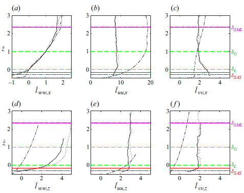
We aim to identify characteristics of the shear-free and shear-dominated surface layers that are similar and dissimilar. To this end, in figure 8 we define a vertical axis $\hat {z}$
that centres on the surface layer and nearby regions to compare integral-scale variations in and near the surface layer in the two very different wall-bounded turbulent flows created in the grid turbulence and TBL experiments
$\hat {z}$
that centres on the surface layer and nearby regions to compare integral-scale variations in and near the surface layer in the two very different wall-bounded turbulent flows created in the grid turbulence and TBL experiments
 \begin{equation} \hat {z} = \frac {z-\delta _L}{\delta _U-\delta _L}. \end{equation}
This normalisation places the lower and upper bounds of the surface layer at $\hat {z} = 0$
and
$\hat {z} = 0$
and $1$
, respectively, for both flows. All integral scales are plotted as a function of
$1$
, respectively, for both flows. All integral scales are plotted as a function of $\hat {z}$
relative to the horizontal integral scales of vertical velocity fluctuation as follows:
$\hat {z}$
relative to the horizontal integral scales of vertical velocity fluctuation as follows:
 \begin{equation} \hat {l}_{\alpha \alpha ,\beta }=\frac {l_{\alpha \alpha ,\beta }-l_{ww,x}(\delta _L)}{l_{ww,x}(\delta _U)-l_{ww,x}(\delta _L)}. \end{equation}
Therefore, in figure 8 all horizontal integral scales of vertical velocity fluctuation, $\hat {l}_{ww,x}$
, pass through
$\hat {l}_{ww,x}$
, pass through $0$
and
$0$
and $1$
at the lower and upper margins of the surface layer by construction. For vertical velocity fluctuations, the horizontal integral scales of the grid and TBL flows overlap at
$1$
at the lower and upper margins of the surface layer by construction. For vertical velocity fluctuations, the horizontal integral scales of the grid and TBL flows overlap at $\hat {z}=0$
and
$\hat {z}=0$
and $1$
and throughout the surface layer due to linear scaling.
$1$
and throughout the surface layer due to linear scaling.
This is not the case, however, with the other integral scales. Figure 8 shows that the two grid-turbulence SFSL cases agree well for normalised streamwise length scales, while the correlations in the vertical direction show larger differences while still trending together. In the vertical what is plotted is the correlation length as a function of starting $z$
location. The vertical correlation of the vertical fluctuating velocity,
$z$
location. The vertical correlation of the vertical fluctuating velocity, $l_{ww,z}$
, in particular, appears to suggest overall larger vertical correlation lengths relative to the thickness of the surface layers with the smaller grid. Whether this difference reflects a different turbulence structure, a Reynolds number effect or is related to the measure used to quantify coherence in inhomogeneous directions (2.3), is unclear.
$l_{ww,z}$
, in particular, appears to suggest overall larger vertical correlation lengths relative to the thickness of the surface layers with the smaller grid. Whether this difference reflects a different turbulence structure, a Reynolds number effect or is related to the measure used to quantify coherence in inhomogeneous directions (2.3), is unclear.
In context with the previous observation, note from figure 4 and table 5 that, while the thicknesses of the SML and SFSL are smaller with the smaller grid, the ratio of SFSL to SML thickness is the same. Interestingly, figure 8 shows that, while the $\hat {z}$
normalisation on the SFSL thickness collapses both the height of the surface-modulated layers for the large and small grids (SML, magenta lines), it also collapses the thickness of the surface-adjacent layer (SAS, red lines), suggesting a relative gap between
$\hat {z}$
normalisation on the SFSL thickness collapses both the height of the surface-modulated layers for the large and small grids (SML, magenta lines), it also collapses the thickness of the surface-adjacent layer (SAS, red lines), suggesting a relative gap between $\delta _{SAS}$
and
$\delta _{SAS}$
and $\delta _L$
set by the largest surface-layer eddies in the vertical. Based on the definition
$\delta _L$
set by the largest surface-layer eddies in the vertical. Based on the definition $\delta _{SAS}^+=40$
, designed to capture most (but not all) of the turbulence production rate, the relative gap between the SAS and the SDSL in the TBL is wider than between the SAS and SFSL in the grid-turbulence flows, as previously discussed (§ 3.2). The separation between
$\delta _{SAS}^+=40$
, designed to capture most (but not all) of the turbulence production rate, the relative gap between the SAS and the SDSL in the TBL is wider than between the SAS and SFSL in the grid-turbulence flows, as previously discussed (§ 3.2). The separation between $\delta _{SML}$
and
$\delta _{SML}$
and $\delta _U$
is much greater for the TBL than for the grid-turbulence cases, so that the surface-layer scaling does not collapse the SML as in the grid-turbulence cases.
$\delta _U$
is much greater for the TBL than for the grid-turbulence cases, so that the surface-layer scaling does not collapse the SML as in the grid-turbulence cases.
As previously observed, figures 8(a)–8(f) as a group show clearly that only coherence lengths of vertical fluctuating velocity in the streamwise direction increase linearly with wall-normal distance from the surface in all flows. The only other coherence length that increases with distance from the surface in all three datasets is the correlation of vertical velocity fluctuations in the vertical. This observation is consistent with the hypothesis that the essential coherence character of the surface layer is associated with blockage over wall-normal fluctuations by the impermeable surface. As mentioned above, the lack of linearity in $l_{ww,z}(z)$
may reflect, in part, the impact of inhomogeniety in the vertical on the coherence measure (2.3).
$l_{ww,z}(z)$
may reflect, in part, the impact of inhomogeniety in the vertical on the coherence measure (2.3).
The other global observation that is apparent from the group of figures is that, whereas for the SFSL flows some integral scales may increase, decrease, or remain constant with distance from the surface, in the TBL SDSL flow all integral scales increase with distance from the surface, with linearity in $l_{ww,x}(z)$
as a special case. As will be discussed in coming sections, this universal behaviour likely reflects the existence of turbulence production above the SAS and throughout the surface layer as a consequence of shear in the SDSL in comparison with the SFSL. Although the integral length scale of vertical velocity in the cross-stream direction,
$l_{ww,x}(z)$
as a special case. As will be discussed in coming sections, this universal behaviour likely reflects the existence of turbulence production above the SAS and throughout the surface layer as a consequence of shear in the SDSL in comparison with the SFSL. Although the integral length scale of vertical velocity in the cross-stream direction, $l_{ww,y}$
, is not available in the present datasets, the RDT analysis of Hunt & Carlotti (Reference Hunt and Carlotti2001) suggests that
$l_{ww,y}$
, is not available in the present datasets, the RDT analysis of Hunt & Carlotti (Reference Hunt and Carlotti2001) suggests that $l_{ww,y}$
displays linear scaling with distance from the surface similar to that observed in
$l_{ww,y}$
displays linear scaling with distance from the surface similar to that observed in $l_{ww,x}(z)$
.
$l_{ww,x}(z)$
.
In the grid-turbulence SFSL, the integral length scale of the streamwise velocity component in the streamwise direction, $l_{uu,x}$
, is relatively constant with
$l_{uu,x}$
, is relatively constant with $z$
in the SFSL, while the integral scale of the cross-stream velocity in the streamwise direction,
$z$
in the SFSL, while the integral scale of the cross-stream velocity in the streamwise direction, $l_{vv,x}$
, shows a clear increase towards the surface. In figure 8 from TH77, predictions from the HG78 RDT theory are compared with their grid-turbulence experimental results for
$l_{vv,x}$
, shows a clear increase towards the surface. In figure 8 from TH77, predictions from the HG78 RDT theory are compared with their grid-turbulence experimental results for $l_{uu,x}(z)$
. Whereas our grid-turbulence experiments in figure 8 show roughly uniform
$l_{uu,x}(z)$
. Whereas our grid-turbulence experiments in figure 8 show roughly uniform $l_{uu,x}$
through the SFSL, there is an indication, with both grids, that
$l_{uu,x}$
through the SFSL, there is an indication, with both grids, that $l_{uu,x}(z)$
decreases towards the surface beginning in the lower SFSL and into the SAS. The RDT theory also predicts a reduction, but it is a somewhat greater and more gradual reduction that initiates near the upper margin of a linear variation in
$l_{uu,x}(z)$
decreases towards the surface beginning in the lower SFSL and into the SAS. The RDT theory also predicts a reduction, but it is a somewhat greater and more gradual reduction that initiates near the upper margin of a linear variation in $l_{ww,x}$
observed in the overlaid TH77 experimental data. However, the reduction in
$l_{ww,x}$
observed in the overlaid TH77 experimental data. However, the reduction in $l_{uu,x}$
towards the surface shown in TH77 data initiates in the lower margin of the linear region more consistent with our figure 8.
$l_{uu,x}$
towards the surface shown in TH77 data initiates in the lower margin of the linear region more consistent with our figure 8.
One might suspect that in the SFSL the reduction towards the surface in $l_{ww,x}$
together with increasing
$l_{ww,x}$
together with increasing $l_{vv,x}$
may indirectly reflect continuity (§ 4.3). On the other hand, it is curious that, whereas we later show in figure 11 that the normalised variances of the streamwise and transverse velocity fluctuations increase equivalently towards the surface in the lower SFSL consistent with the HG78 theory for isotropic turbulence, the streamwise integral scale of transverse velocity in figure 8 clearly increases towards the surface in the lower SFSL while the integral scale of streamwise velocity clearly does not. The same is true in the TH77 data.
$l_{vv,x}$
may indirectly reflect continuity (§ 4.3). On the other hand, it is curious that, whereas we later show in figure 11 that the normalised variances of the streamwise and transverse velocity fluctuations increase equivalently towards the surface in the lower SFSL consistent with the HG78 theory for isotropic turbulence, the streamwise integral scale of transverse velocity in figure 8 clearly increases towards the surface in the lower SFSL while the integral scale of streamwise velocity clearly does not. The same is true in the TH77 data.
In stark contrast with the SFSL grid-turbulence variations just discussed, in the TBL $l_{uu,x}(z)$
increases strongly and consistently from the surface and through the SDSL, reaching a peak near the upper margin of the SDSL. This, we argue, is a consequence of the existence of mean shear rate and turbulence production, which peaks at
$l_{uu,x}(z)$
increases strongly and consistently from the surface and through the SDSL, reaching a peak near the upper margin of the SDSL. This, we argue, is a consequence of the existence of mean shear rate and turbulence production, which peaks at $z^+\approx 11$
, within the SAS and well below the SDSL. Turbulence eddies created below the SDSL are distorted both by interactions with the impermeable surface and by mean shear as they move through the surface layer and into the upper regions of the TBL. It is well understood that mean shear rate causes coherent structure in the fluctuating streamwise velocity to elongate in the streamwise direction (Lee et al. Reference Lee, Kim and Moin1990) so that the
$z^+\approx 11$
, within the SAS and well below the SDSL. Turbulence eddies created below the SDSL are distorted both by interactions with the impermeable surface and by mean shear as they move through the surface layer and into the upper regions of the TBL. It is well understood that mean shear rate causes coherent structure in the fluctuating streamwise velocity to elongate in the streamwise direction (Lee et al. Reference Lee, Kim and Moin1990) so that the $u'$
eddies elongate and the streamwise coherence length increases from the lower to upper SDSL where mean shear rate decreases like
$u'$
eddies elongate and the streamwise coherence length increases from the lower to upper SDSL where mean shear rate decreases like $1/z$
. Whereas
$1/z$
. Whereas $l_{uu,x}(z)$
increases strongly through the SDSL,
$l_{uu,x}(z)$
increases strongly through the SDSL, $l_{vv,x}$
increases only gradually, through the SDSL and into the upper TBL.
$l_{vv,x}$
increases only gradually, through the SDSL and into the upper TBL.
What is particularly interesting in the observations above is that, independent of the existence of mean shear with corresponding turbulence production and the distortion/elongation of turbulence eddies, and independent of the increase or not of other integral scales, only the integral scales of vertical fluctuating velocity increase with distance from the surface in all three experiments. Furthermore, only the horizontal integral scales of vertical fluctuating velocity increase linearly with $z$
in a region we define as a surface layer. Whereas in the current experiments it was not possible to measure transverse correlations, linear growth of the integral length scales of vertical fluctuating velocity in both horizontal directions was identified by Apostolidis et al. (Reference Apostolidis, Laval and Vassilicos2022) in direct numeric simulation channel flow data. The observation that only the vertical fluctuating velocity has correlation lengths that scale on wall-normal distance strongly supports the hypothesis that the general mechanisms that create a surface layer are associated with blockage of vertical velocity at an impermeable surface.
$z$
in a region we define as a surface layer. Whereas in the current experiments it was not possible to measure transverse correlations, linear growth of the integral length scales of vertical fluctuating velocity in both horizontal directions was identified by Apostolidis et al. (Reference Apostolidis, Laval and Vassilicos2022) in direct numeric simulation channel flow data. The observation that only the vertical fluctuating velocity has correlation lengths that scale on wall-normal distance strongly supports the hypothesis that the general mechanisms that create a surface layer are associated with blockage of vertical velocity at an impermeable surface.
4. Differences between the shear-free and shear-dominated surface layers
In this section we continue the comparison of surface layers in a shear-free vs. shear-dominated environment to elucidate common, potentially generalisable, characteristics in contrast with fundamental differences. Because a fundamental difference between these flows is the existence, or not, of finite mean shear rate through the surface layer, we compare turbulence production rates in the next section, followed by comparisons of velocity variances in context with blockage and theory. We close with an analysis of the central role of continuity in the relationship between linear variation of integral scale $z$
and the vertical velocity variance.
$z$
and the vertical velocity variance.
For the two SFSL grid cases, the wall-normal profiles of (a) normalised mean velocity, (b) mean shear rate, (c) Reynolds shear stress and (d) turbulence production rate against $\hat {z}$
. —–, large grid;
$\hat {z}$
. —–, large grid; $\cdots \cdots$
, small grid. The horizontal lines indicate
$\cdots \cdots$
, small grid. The horizontal lines indicate $\delta _U$
,
$\delta _U$
, $\delta _L$
,
$\delta _L$
, $\delta _{SML}$
and
$\delta _{SML}$
and $\delta _{SAS}$
as labelled in the figure.
$\delta _{SAS}$
as labelled in the figure.
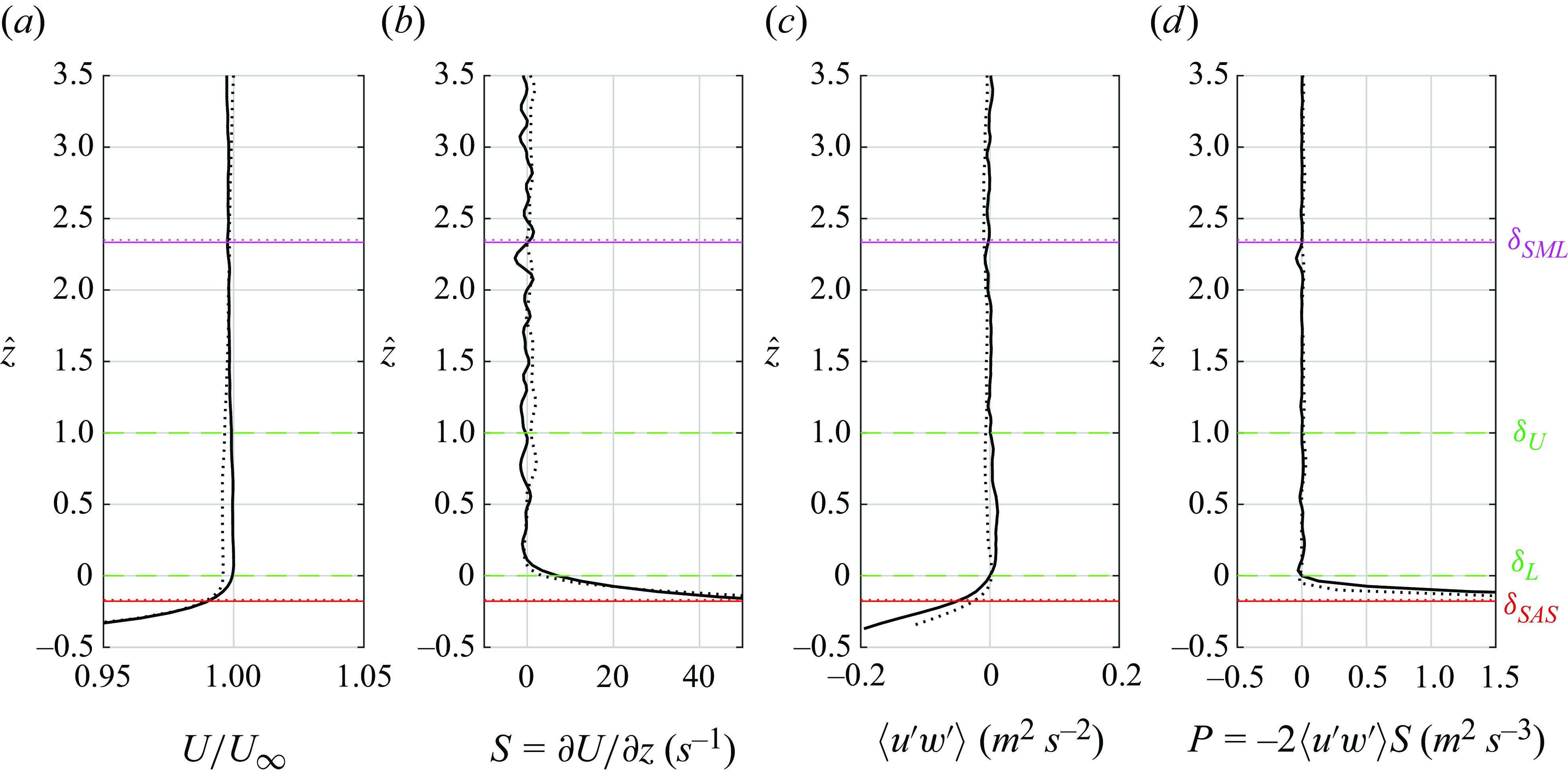
For the SDSL TBL case, the wall-normal profiles of (a) normalised mean velocity, (b) mean shear rate, (c) Reynolds shear stress and (d) turbulence production rate. The horizontal lines indicate $\delta _U$
,
$\delta _U$
, $\delta _L$
and
$\delta _L$
and $\delta _{SAS}$
, as labelled in the figure.
$\delta _{SAS}$
, as labelled in the figure.

4.1. Turbulence production rate
The two classes of wall-bounded turbulent flow considered here have fundamentally different mean shear rate and shear-generated turbulence production-rate characteristics as shown in figures 9 and 10, where normalised mean velocity, mean shear rate, Reynolds shear stress and turbulent production rate are plotted against the normalised wall-normal distance, $\hat {z}$
(3.2). In the grid-turbulence flows, mean shear, Reynolds shear stress and turbulence production are confined to the SAS, which in this case is a highly non-canonical boundary layer in which the turbulence fluctuations generated very near the surface are confined. The HG78 model predicts that if the SAS is sufficiently thin, it does not impact the suppression of vertical velocity by surface impermeability, which we argued in § 3.1 is also the case in both the TH77 and the current experiments.
$\hat {z}$
(3.2). In the grid-turbulence flows, mean shear, Reynolds shear stress and turbulence production are confined to the SAS, which in this case is a highly non-canonical boundary layer in which the turbulence fluctuations generated very near the surface are confined. The HG78 model predicts that if the SAS is sufficiently thin, it does not impact the suppression of vertical velocity by surface impermeability, which we argued in § 3.1 is also the case in both the TH77 and the current experiments.
Interestingly, figure 9 shows that mean shear rate, Reynolds shear stress and turbulence production rate all decrease in the vertical direction from the upper margin of the SAS to reach zero precisely at the lower margin of the SFSL, where $l_{ww,x}$
initiates a linear increase with
$l_{ww,x}$
initiates a linear increase with $z$
. The SFSL, as indicated by dashed green lines, exists in the region of zero shear-induced turbulence production rate. The observation that the two grid flow profiles and the locations of
$z$
. The SFSL, as indicated by dashed green lines, exists in the region of zero shear-induced turbulence production rate. The observation that the two grid flow profiles and the locations of $\delta _{SAS}$
and
$\delta _{SAS}$
and $\delta _{SML}$
collapse when scaled on the depth of the SFSL suggests that the initiation of a SFSL outside a SAS that confines near-wall turbulence production and Reynolds shear stress is a generalisable result for the influence of a surface on turbulence eddies that originated away from the surface. However, the fact that the canonical TBL contains a surface layer within a region in which mean shear rate, turbulence production rate and Reynolds shear stress are non-zero, as shown in figure 10, implies that the lack of mean shear and turbulence production is not a general requirement for the existence of a surface layer. This leads to the question of what is the fundamental mechanism that allows the surface layer to exist both in the presence of turbulence production in the TBL SDSL and in the absence of turbulence production in the grid-turbulence SFSL.
$\delta _{SML}$
collapse when scaled on the depth of the SFSL suggests that the initiation of a SFSL outside a SAS that confines near-wall turbulence production and Reynolds shear stress is a generalisable result for the influence of a surface on turbulence eddies that originated away from the surface. However, the fact that the canonical TBL contains a surface layer within a region in which mean shear rate, turbulence production rate and Reynolds shear stress are non-zero, as shown in figure 10, implies that the lack of mean shear and turbulence production is not a general requirement for the existence of a surface layer. This leads to the question of what is the fundamental mechanism that allows the surface layer to exist both in the presence of turbulence production in the TBL SDSL and in the absence of turbulence production in the grid-turbulence SFSL.
The fundamental difference between the two classes of flow is in the origin of the turbulence that is subsequently distorted in a similar manner in both flows so as to produce linear growth in $l_{ww,x}(z)$
in an inertia-dominated surface layer. In the grid-turbulence experiments the SFSL is created within turbulence eddies that were generated away from the surface and interact with the impermeable surface through a SAS. This SAS must be sufficiently thin, relative to the free-stream integral scale, that the eddies outside the SAS in the SFSL can respond directly to blockage at the surface (note that
$l_{ww,x}(z)$
in an inertia-dominated surface layer. In the grid-turbulence experiments the SFSL is created within turbulence eddies that were generated away from the surface and interact with the impermeable surface through a SAS. This SAS must be sufficiently thin, relative to the free-stream integral scale, that the eddies outside the SAS in the SFSL can respond directly to blockage at the surface (note that $\delta _L\approx 1.4\delta _{SAS}$
, table 5). This blockage impacts turbulence eddy structure over a sufficiently extended distance from the surface to create measurable linear growth in the horizontal integral scale of vertical fluctuations over a distance that scales on free-stream turbulence eddy size. In the TBL, however, the turbulence eddies that are modulated by the surface to create the SDSL originate very close to the surface below the lower margin of the SDSL in the vicinity of peak production rate at
$\delta _L\approx 1.4\delta _{SAS}$
, table 5). This blockage impacts turbulence eddy structure over a sufficiently extended distance from the surface to create measurable linear growth in the horizontal integral scale of vertical fluctuations over a distance that scales on free-stream turbulence eddy size. In the TBL, however, the turbulence eddies that are modulated by the surface to create the SDSL originate very close to the surface below the lower margin of the SDSL in the vicinity of peak production rate at $z^+\approx 11$
. In the
$z^+\approx 11$
. In the $\hat {z}$
coordinates of figure 10, peak production rate occurs at
$\hat {z}$
coordinates of figure 10, peak production rate occurs at $\hat {z}\approx -0.51$
, well below
$\hat {z}\approx -0.51$
, well below $\delta _{SAS}$
and, especially,
$\delta _{SAS}$
and, especially, $\delta _L$
. Furthermore, we estimate the shear production-rate value at
$\delta _L$
. Furthermore, we estimate the shear production-rate value at $\delta _{SAS}$
to be approximately one fifth of the peak value and note that
$\delta _{SAS}$
to be approximately one fifth of the peak value and note that $\delta _L\approx 2\delta _{SAS}$
(table 5). As the turbulence eddies that were generated very near the surface fill the boundary layer downstream, they pass through the surface layer where mean shear rate in the surface layer (figure 10
b) elongates the eddies to produce the continual increase in
$\delta _L\approx 2\delta _{SAS}$
(table 5). As the turbulence eddies that were generated very near the surface fill the boundary layer downstream, they pass through the surface layer where mean shear rate in the surface layer (figure 10
b) elongates the eddies to produce the continual increase in $l_{uu,x}$
with
$l_{uu,x}$
with $z$
through the SDSL, as observed in figure 8(b) (and previously discussed in § 3.3).
$z$
through the SDSL, as observed in figure 8(b) (and previously discussed in § 3.3).
Wall-normal variations in normalised component velocity variances in the grid-turbulence–surface experiments for (a) the large grid and (b) the small grid, plotted against $\hat {z}$
to centre on the SFSL. Also plotted are the normalised sum of the horizontal variances,
$\hat {z}$
to centre on the SFSL. Also plotted are the normalised sum of the horizontal variances, $\langle u_h'^2 \rangle$
, and the normalised sum of the three variances,
$\langle u_h'^2 \rangle$
, and the normalised sum of the three variances, $\langle q^2 \rangle$
. All variances are normalised by their values in the free stream (see table 1 for relative variances). The horizontal lines indicate
$\langle q^2 \rangle$
. All variances are normalised by their values in the free stream (see table 1 for relative variances). The horizontal lines indicate $\delta _U$
,
$\delta _U$
, $\delta _L$
,
$\delta _L$
, $\delta _{SML}$
and
$\delta _{SML}$
and $\delta _{SAS}$
, as labelled in the figure. The location of the surface is: (a)
$\delta _{SAS}$
, as labelled in the figure. The location of the surface is: (a) $\hat {z} = -0.59$
and (b)
$\hat {z} = -0.59$
and (b) $\hat {z} = -0.64$
.
$\hat {z} = -0.64$
.

Wall-normal variations in velocity variances in the TBL normalised by the corresponding component variances at the upper margin of the SDSL, $\delta _U$
, plotted against
$\delta _U$
, plotted against $\hat {z}$
to centre on the SDSL. Like figure 11, also plotted are the sum of the horizontal fluctuations,
$\hat {z}$
to centre on the SDSL. Like figure 11, also plotted are the sum of the horizontal fluctuations, $\langle u_h'^2\rangle$
and the sum of all three variances,
$\langle u_h'^2\rangle$
and the sum of all three variances, $\langle q^2\rangle$
. The horizontal lines indicate
$\langle q^2\rangle$
. The horizontal lines indicate $\delta _U$
,
$\delta _U$
, $\delta _L$
and
$\delta _L$
and $\delta _{SAS}$
. At
$\delta _{SAS}$
. At $\delta _U$
,
$\delta _U$
, $\langle u'^2\rangle /\langle w'^2\rangle = 3.39$
and
$\langle u'^2\rangle /\langle w'^2\rangle = 3.39$
and $\langle u'^2\rangle /\langle v'^2\rangle = 2.28$
. The location of the surface is
$\langle u'^2\rangle /\langle v'^2\rangle = 2.28$
. The location of the surface is $\hat {z} = -0.58$
.
$\hat {z} = -0.58$
.
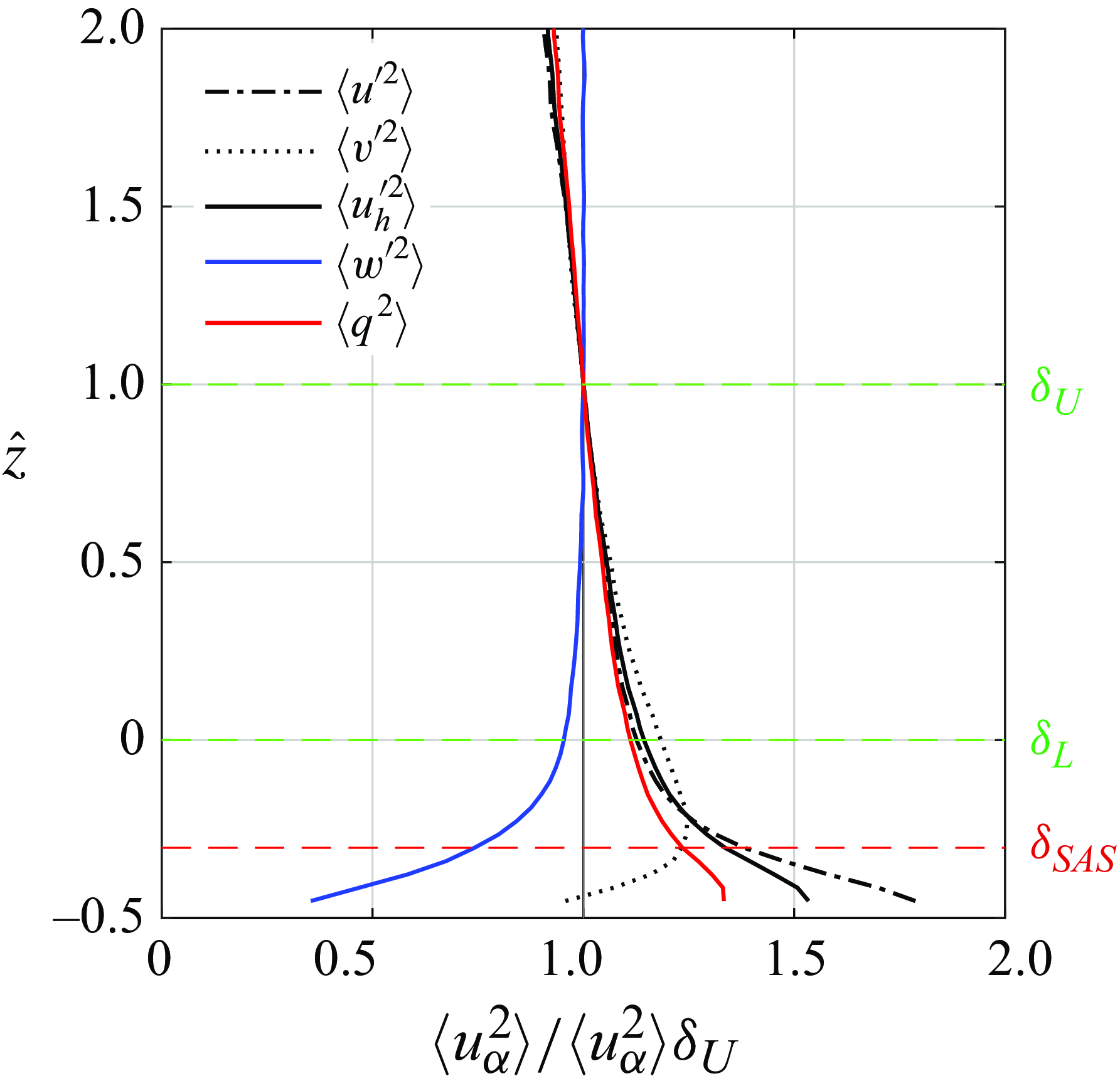
4.2. Impacts of the surface on the variations in velocity variances
The relative variations in the variances of the fluctuating velocity components through the SFSL and SDSL are presented in figures 11 and 12. Specifically, we compare the wall-normal variations of normalised velocity variances, $\langle u'^2\rangle$
,
$\langle u'^2\rangle$
, $\langle w'^2\rangle$
and
$\langle w'^2\rangle$
and $\langle v'^2\rangle$
, centred on the surface layer using the normalised vertical height,
$\langle v'^2\rangle$
, centred on the surface layer using the normalised vertical height, $\hat {z}$
in (3.2). Also plotted are the normalised variances of the ‘horizontal’ velocity vector in the plane parallel to the surface,
$\hat {z}$
in (3.2). Also plotted are the normalised variances of the ‘horizontal’ velocity vector in the plane parallel to the surface, $\langle u'^2_h\rangle =\langle u'^2\rangle +\langle v'^2\rangle$
, and twice the turbulent kinetic energy,
$\langle u'^2_h\rangle =\langle u'^2\rangle +\langle v'^2\rangle$
, and twice the turbulent kinetic energy, $\langle q^2\rangle =\langle u'^2\rangle +\langle v'^2\rangle +\langle w'^2\rangle$
. Each variance is plotted normalised. For the grid-turbulence cases we normalise with values in the free stream, while in the TBL experiments we normalise with the values at the upper margin of the SDSL,
$\langle q^2\rangle =\langle u'^2\rangle +\langle v'^2\rangle +\langle w'^2\rangle$
. Each variance is plotted normalised. For the grid-turbulence cases we normalise with values in the free stream, while in the TBL experiments we normalise with the values at the upper margin of the SDSL, $\delta _U$
.
$\delta _U$
.
In and surrounding the SFSL created by grid-turbulence–surface interactions, there is consistency in the $z$
variations of the normalised component variances between the large and small grids shown in figure 11. There is also consistency between the current results above
$z$
variations of the normalised component variances between the large and small grids shown in figure 11. There is also consistency between the current results above $\delta _{SAS}$
, the experimental results obtained by TH77 and the theory of HG78, where the latter two are compared in figure 5 of HG78. As analysed in detail in § 4.3, data and theory all demonstrate a trade-off between the vertical and horizontal velocity variances in the SFSL. Whereas
$\delta _{SAS}$
, the experimental results obtained by TH77 and the theory of HG78, where the latter two are compared in figure 5 of HG78. As analysed in detail in § 4.3, data and theory all demonstrate a trade-off between the vertical and horizontal velocity variances in the SFSL. Whereas $\langle w'^2 \rangle$
decreases through the entire surface-modified region towards zero at the surface, it decreases more rapidly from the upper to lower margins of the SFSL. The more rapid decrease towards the lower margin of the SFSL coincides with an increase in horizontal velocity variance that continues into the SAS, a trade-off also clear in the HG78 theory and TH77 data.
$\langle w'^2 \rangle$
decreases through the entire surface-modified region towards zero at the surface, it decreases more rapidly from the upper to lower margins of the SFSL. The more rapid decrease towards the lower margin of the SFSL coincides with an increase in horizontal velocity variance that continues into the SAS, a trade-off also clear in the HG78 theory and TH77 data.
Qualitatively consistent with the HG78 theory, figure 11 shows a decrease in turbulent kinetic energy ( $\langle q^2\rangle /2$
) followed by an increase from the lower margins of the SFSL towards
$\langle q^2\rangle /2$
) followed by an increase from the lower margins of the SFSL towards $\delta _{SAS}$
. However, because the HG78 theory applies in the limit of an infinitesimally thin SAS, the vertical velocity variance approaches zero due to surface impermeability at the upper margin of their viscous SAS. By contrast, in the current SFSL grid-turbulence experiments the SAS is relatively thick, 26 %–32
$\delta _{SAS}$
. However, because the HG78 theory applies in the limit of an infinitesimally thin SAS, the vertical velocity variance approaches zero due to surface impermeability at the upper margin of their viscous SAS. By contrast, in the current SFSL grid-turbulence experiments the SAS is relatively thick, 26 %–32 $\%$
of
$\%$
of $l_{uu,x_\infty }$
(table 5). Consequently, the vertical velocity variance at the lower boundary of the SFSL is relatively large, approximately
$l_{uu,x_\infty }$
(table 5). Consequently, the vertical velocity variance at the lower boundary of the SFSL is relatively large, approximately $50\%$
of the free-stream value. Figure 11 shows that, when normalised by the free-stream values, the streamwise, cross-stream and horizontal velocity variances coincide throughout the SML. These horizontal variances decrease from the upper margin of the SML to a minor minimum slightly below the free-stream values near the upper margin of the surface layer, consistent with the HG78 theory, before transitioning to increasing
$50\%$
of the free-stream value. Figure 11 shows that, when normalised by the free-stream values, the streamwise, cross-stream and horizontal velocity variances coincide throughout the SML. These horizontal variances decrease from the upper margin of the SML to a minor minimum slightly below the free-stream values near the upper margin of the surface layer, consistent with the HG78 theory, before transitioning to increasing $\langle u'^2_h \rangle$
towards and below the lower margin of the SFSL.
$\langle u'^2_h \rangle$
towards and below the lower margin of the SFSL.
In comparison with figure 11 for the SFSL, figure 12 shows both similarities and differences in the variations of the normalised variances surrounding the SDSL of the TBL, differences that can be understood in context with the discussions surrounding turbulence production in § 4.1 above. The vertical velocity variance, in blue, decreases relatively slowly in the surface-layer region compared with the transitional layer approaching the SAS below, where the variance decreases sharply towards zero at the impermeable surface. In contrast with the SFSL, vertical velocity variance decreases from the upper to lower margins of the SDSL (figure 12) much more slowly than through the SFSL (figure 11), while the streamwise and cross-stream velocity variances (in black) increase towards the surface within the SDSL more rapidly than within the SFSL. In the grid-turbulence flows, the two normalised horizontal variances vary similarly through the SFSL. In the TBL, whereas the horizontal velocity variance is dominated by the streamwise velocity fluctuations, the transverse variance has a somewhat different variation than the streamwise component, especially in the SAS region.
In comparison with the SFSL we attribute the more rapid increase in streamwise velocity variance from the upper to lower margins of the SDSL to turbulence production in this region (§ 4.1). Shear-driven turbulence production enters the streamwise fluctuating velocity directly before being transferred into the cross-stream and vertical components through pressure–strain-rate inter-component energy transfer. However, because both peak production rate of streamwise variance and streamwise velocity variance occur well below $\delta _L$
(
$\delta _L$
( $z+\approx 11$
and
$z+\approx 11$
and $15$
, respectively), the variations in transverse and vertical velocity variances through the SDSL are likely driven both by inter-component energy transfer and the vertical transport of turbulence eddies into the SDSL region from below. In the SFSL where turbulence production does not exist, however, the increase in the horizontal velocity variance from the upper to lower boundary of the surface layer is likely associated with incompressibility, as discussed in the following section (§ 4.3). Also similar to the SFSL results in figure 11, whereas the HG78 theory predicts a decrease in
$15$
, respectively), the variations in transverse and vertical velocity variances through the SDSL are likely driven both by inter-component energy transfer and the vertical transport of turbulence eddies into the SDSL region from below. In the SFSL where turbulence production does not exist, however, the increase in the horizontal velocity variance from the upper to lower boundary of the surface layer is likely associated with incompressibility, as discussed in the following section (§ 4.3). Also similar to the SFSL results in figure 11, whereas the HG78 theory predicts a decrease in $\langle w'^2\rangle$
towards zero together with an increase in
$\langle w'^2\rangle$
towards zero together with an increase in $\langle u'^2\rangle$
without turbulence production, normalised
$\langle u'^2\rangle$
without turbulence production, normalised $\langle w'^2\rangle$
in the TBL approaches a value at the upper margin of the SAS that is even larger than that for the fixed-wall SFSL of figure 11. This suggests that wall blockage of vertical velocity at the SAS of the TBL is partially masked by production and inter-component energy transfer from streamwise to vertical turbulence fluctuations in the region below the SDSL, where
$\langle w'^2\rangle$
in the TBL approaches a value at the upper margin of the SAS that is even larger than that for the fixed-wall SFSL of figure 11. This suggests that wall blockage of vertical velocity at the SAS of the TBL is partially masked by production and inter-component energy transfer from streamwise to vertical turbulence fluctuations in the region below the SDSL, where $\langle u'^2\rangle$
is most strongly produced by mean shear rate.
$\langle u'^2\rangle$
is most strongly produced by mean shear rate.
Related to these observations, we note that whereas vertical velocity variance decreases from the upper to lower margins of the surface layer in both the SFSL and SDSL, turbulent kinetic energy decreases in the SFSL but increases in the SDSL due to the existence of turbulence production. What is particularly interesting is that even with the generation of streamwise velocity fluctuations by shear production and the transfer of variance into vertical and transverse velocity fluctuations through correlations between pressure and strain-rate fluctuations, surface layers with linear increases with $z$
in the horizontal coherence length of vertical fluctuations are created in both flows.
$z$
in the horizontal coherence length of vertical fluctuations are created in both flows.
An attempt to account for these observations may follow from a simple spectral model in a horizontally homogeneous channel flow. Perry et al. (Reference Perry, Henbest and Chong1986) argued that, because of blocking at the surface, primarily only eddies of size $O(z)$
contribute to
$O(z)$
contribute to $w'$
motions whereas eddies of size larger than
$w'$
motions whereas eddies of size larger than $O(z)$
contribute primarily to
$O(z)$
contribute primarily to $u'$
and
$u'$
and $v'$
motions but not significantly to
$v'$
motions but not significantly to $w'$
motions for
$w'$
motions for $z\ll \delta$
. The one-dimensional streamwise energy spectrum
$z\ll \delta$
. The one-dimensional streamwise energy spectrum $E_w (k_{x}, z)$
of fluctuating vertical velocities
$E_w (k_{x}, z)$
of fluctuating vertical velocities $w'$
at distance
$w'$
at distance $z$
from the wall is therefore modelled as approximately constant up to
$z$
from the wall is therefore modelled as approximately constant up to $k_{x}\sim 1/z$
, hence equal to
$k_{x}\sim 1/z$
, hence equal to $E_w (k_{x}=0 , z)$
for
$E_w (k_{x}=0 , z)$
for $k_{x} \lt O(1/z)$
. Assuming, following Perry et al. (Reference Perry, Henbest and Chong1986), that eddies of size smaller than distance
$k_{x} \lt O(1/z)$
. Assuming, following Perry et al. (Reference Perry, Henbest and Chong1986), that eddies of size smaller than distance $z$
from the wall are in approximate Kolmogorov 1941 (K41) equilibrium, we may write
$z$
from the wall are in approximate Kolmogorov 1941 (K41) equilibrium, we may write $E_w (k_{x},z) \sim \epsilon ^{2/3}k_{x}^{-5/3}$
for some range of wavenumbers
$E_w (k_{x},z) \sim \epsilon ^{2/3}k_{x}^{-5/3}$
for some range of wavenumbers $k_{x}$
larger than
$k_{x}$
larger than $O(1/z)$
. Matching at
$O(1/z)$
. Matching at $k_{x} = O(1/z)$
gives
$k_{x} = O(1/z)$
gives $E_w(k_{x}=0 , z) \sim \epsilon ^{2/3} z^{5/3}$
. Integrating
$E_w(k_{x}=0 , z) \sim \epsilon ^{2/3} z^{5/3}$
. Integrating $E_w (k_{x},z)$
over all
$E_w (k_{x},z)$
over all $k_x$
yields a contribution
$k_x$
yields a contribution $\sim (\epsilon z)^{2/3}$
to
$\sim (\epsilon z)^{2/3}$
to $\langle w'^{2} \rangle$
from
$\langle w'^{2} \rangle$
from $k_{x}=0$
to
$k_{x}=0$
to $k_{x} \sim 1/z$
and a contribution to
$k_{x} \sim 1/z$
and a contribution to $\langle w'^{2} \rangle$
from larger
$\langle w'^{2} \rangle$
from larger $k_x$
which is bounded from above by a term
$k_x$
which is bounded from above by a term $\sim (\epsilon z)^{2/3}$
and is in fact proportional to
$\sim (\epsilon z)^{2/3}$
and is in fact proportional to $(\epsilon z)^{2/3}$
rather than just bounded by it if the Reynolds number is high enough to support a significant K41 inertial range. We can therefore consider
$(\epsilon z)^{2/3}$
rather than just bounded by it if the Reynolds number is high enough to support a significant K41 inertial range. We can therefore consider $\langle w'^{2} \rangle \sim (\epsilon z)^{2/3}$
to be a good approximation even at Reynolds numbers that are not so high. In the SDSL of the TBL, which coincides with the log layer (figure 6), we may expect
$\langle w'^{2} \rangle \sim (\epsilon z)^{2/3}$
to be a good approximation even at Reynolds numbers that are not so high. In the SDSL of the TBL, which coincides with the log layer (figure 6), we may expect $\epsilon$
to approximately balance production and therefore scale approximately as
$\epsilon$
to approximately balance production and therefore scale approximately as $u_{\tau }^{3}/z$
. Hence,
$u_{\tau }^{3}/z$
. Hence, $\langle w'^{2} \rangle$
is roughly constant with
$\langle w'^{2} \rangle$
is roughly constant with $z$
in the high Reynolds number TBL (more so at the upper part of the SDSL where Kolmogorov spectra will be better defined than at the lower part). In the SFSL,
$z$
in the high Reynolds number TBL (more so at the upper part of the SDSL where Kolmogorov spectra will be better defined than at the lower part). In the SFSL, $\epsilon$
may be assumed approximately homogeneous, hence independent of
$\epsilon$
may be assumed approximately homogeneous, hence independent of $z$
, and therefore
$z$
, and therefore $\langle w'^{2} \rangle \sim z^{2/3}$
. The overall shape of
$\langle w'^{2} \rangle \sim z^{2/3}$
. The overall shape of $E_w (k_{x}, z)$
assumed by Perry et al. (Reference Perry, Henbest and Chong1986) can therefore imply, in agreement with our observations, that
$E_w (k_{x}, z)$
assumed by Perry et al. (Reference Perry, Henbest and Chong1986) can therefore imply, in agreement with our observations, that $\langle w'^{2}\rangle$
decreases from the upper to the lower margins of the surface layer much more slowly for the SDSL than for the SFSL. We note (Tennekes & Lumley Reference Tennekes and Lumley1972) that the
$\langle w'^{2}\rangle$
decreases from the upper to the lower margins of the surface layer much more slowly for the SDSL than for the SFSL. We note (Tennekes & Lumley Reference Tennekes and Lumley1972) that the $k_{x}=0$
limit of
$k_{x}=0$
limit of $\pi E_w (k_{x},z)$
is the integral of the non-normalised two-point correlation of
$\pi E_w (k_{x},z)$
is the integral of the non-normalised two-point correlation of $w'$
, that is,
$w'$
, that is, $C_{ww,x}(z)\equiv l_{ww,x} (z) \langle w'^{2} \rangle$
. The model above for
$C_{ww,x}(z)\equiv l_{ww,x} (z) \langle w'^{2} \rangle$
. The model above for $E_w (k_{x}=0,z)$
and
$E_w (k_{x}=0,z)$
and $\langle w'^{2} \rangle$
therefore also implies that
$\langle w'^{2} \rangle$
therefore also implies that $l_{ww,x} (z)$
scales linearly with z for both the SFSL and the SDSL identically, as observed. Additionally, for the SFSL this model leads to
$l_{ww,x} (z)$
scales linearly with z for both the SFSL and the SDSL identically, as observed. Additionally, for the SFSL this model leads to ${d \langle w'^{2} \rangle / {\rm d} z}\sim \epsilon ^{2/3}z^{-1/3}$
where
${d \langle w'^{2} \rangle / {\rm d} z}\sim \epsilon ^{2/3}z^{-1/3}$
where $\epsilon ^{2/3}$
estimated as
$\epsilon ^{2/3}$
estimated as $\langle u'^{2} \rangle /l_{uu,x}^{2/3}$
from table 1 is approximately 2.3 times larger for the large mesh grid than for the small mesh grid. This difference is consistent with the observation in figure 13 that
$\langle u'^{2} \rangle /l_{uu,x}^{2/3}$
from table 1 is approximately 2.3 times larger for the large mesh grid than for the small mesh grid. This difference is consistent with the observation in figure 13 that $d \langle w'^{2}\rangle / {\rm d} z$
takes 2–2.5 times higher values, on average, in the SFSL with the large mesh grid than with the small mesh grid.
$d \langle w'^{2}\rangle / {\rm d} z$
takes 2–2.5 times higher values, on average, in the SFSL with the large mesh grid than with the small mesh grid.
Wall-normal variations of the terms in (4.3) for (a) the large grid and (b) the small grid, plotted against $\hat {z}$
to centre on the SFSL. The dotted black line is the sum of the calculated terms on the right-hand side of (4.3). The horizontal lines indicate
$\hat {z}$
to centre on the SFSL. The dotted black line is the sum of the calculated terms on the right-hand side of (4.3). The horizontal lines indicate $\delta _U$
,
$\delta _U$
, $\delta _L$
,
$\delta _L$
, $\delta _{SML}$
and
$\delta _{SML}$
and $\delta _{SAS}$
as labelled in the figure.
$\delta _{SAS}$
as labelled in the figure.

4.3. The interplay between vertical and horizontal velocity variances in the surface layer
The theory at the end of the previous section makes clear that linear growth in $l_{ww,x} = C_{ww,x}/\langle w'^2 \rangle$
implies coordinated variation between the vertical gradient
$l_{ww,x} = C_{ww,x}/\langle w'^2 \rangle$
implies coordinated variation between the vertical gradient ${\rm d}C_{ww,x}/{\rm d}z$
of the integral of the non-normalised two-point correlation function,
${\rm d}C_{ww,x}/{\rm d}z$
of the integral of the non-normalised two-point correlation function, $C_{ww,x}$
, and the vertical gradient
$C_{ww,x}$
, and the vertical gradient $d\langle w'^2 \rangle /{\rm d}z$
of vertical velocity variance,
$d\langle w'^2 \rangle /{\rm d}z$
of vertical velocity variance, $\langle w'^2 \rangle$
. As discussed earlier in § 4.2, our results in figure 11, the results of TH77 and the theory of HG78 all demonstrate the existence of a trade-off between a reduction in vertical velocity variance towards the surface that results from blockage of vertical velocity at the surface, and an increase in horizontal velocity variance towards the lower margin of the SFSL and into the SAS. Figures 11 vs. 12 show that the variation of vertical velocity variance with
$\langle w'^2 \rangle$
. As discussed earlier in § 4.2, our results in figure 11, the results of TH77 and the theory of HG78 all demonstrate the existence of a trade-off between a reduction in vertical velocity variance towards the surface that results from blockage of vertical velocity at the surface, and an increase in horizontal velocity variance towards the lower margin of the SFSL and into the SAS. Figures 11 vs. 12 show that the variation of vertical velocity variance with $z$
and the trade-off between vertical and horizontal velocity variances are different in the TBL and grid-turbulence flows. We speculate that this trade-off may be associated with continuity. Therefore, to interpret the blockage-induced vertical derivative of vertical velocity variance in relationship to horizontal velocity variance, and to compare the contributions with the gradient in vertical variance between the shear-free and shear-dominated surface layers, consider the incompressibility constraint
$z$
and the trade-off between vertical and horizontal velocity variances are different in the TBL and grid-turbulence flows. We speculate that this trade-off may be associated with continuity. Therefore, to interpret the blockage-induced vertical derivative of vertical velocity variance in relationship to horizontal velocity variance, and to compare the contributions with the gradient in vertical variance between the shear-free and shear-dominated surface layers, consider the incompressibility constraint
 \begin{equation} \frac {\partial w'}{\partial z}=-\left (\frac {\partial u'}{\partial x}+\frac {\partial v'}{\partial y}\right )=-\boldsymbol {\nabla }_h\cdot \boldsymbol {u}^{\prime}_h, \end{equation}
where $\boldsymbol {u}^{\prime}_h$
is wall-parallel fluctuating velocity vector and
$\boldsymbol {u}^{\prime}_h$
is wall-parallel fluctuating velocity vector and $\nabla _h$
is the wall-parallel gradient operator. This leads to
$\nabla _h$
is the wall-parallel gradient operator. This leads to
 \begin{equation} \frac {d\left \langle w'^{2}\right \rangle }{d z}=\left \langle \frac {\partial w'^{2}}{\partial z}\right \rangle =\left \langle 2w'\frac {\partial w'}{\partial z}\right \rangle =-2\left (\left \langle w'\frac {\partial u'}{\partial x}\right \rangle +\left \langle w'\frac {\partial v'}{\partial y}\right \rangle \right ), \end{equation}
which can be written equivalently as
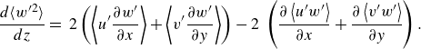 \begin{equation} \frac {d\langle w'^2\rangle }{d z}=\ 2\left (\left \langle u'\frac {\partial w'}{\partial x}\right \rangle +\left \langle v'\frac {\partial w'}{\partial y}\right \rangle \right )-2\ \left (\frac {\partial \left \langle u' w'\right \rangle }{\partial x}+\frac {\partial \left \langle v' w'\right \rangle }{\partial y}\right ). \end{equation}
If the turbulence is quasi-homogeneous in the horizontal, (4.3) is well approximated by
 \begin{equation} \frac {d\langle w'^2\rangle }{d z}\approx \ 2\left (\left \langle u'\frac {\partial w'}{\partial x}\right \rangle +\left \langle v'\frac {\partial w'}{\partial y}\right \rangle \right ) = 2\langle {\boldsymbol {u}^\prime}_h\cdot \nabla _hw'\rangle , \end{equation}
which implies that the vertical gradient of vertical velocity variance is largely driven by the horizontal advection of vertical velocity fluctuations. Therefore, the rate of decrease in vertical velocity variance that results from the blockage of vertical velocity fluctuations at an impermeable surface is expected to be accompanied by an overall increase in horizontal velocity fluctuations due to incompressibility. It is largely for this reason, we argue, that the more rapid decrease in vertical velocity variance toward the surface in the SFSL is associated with increasing horizontal velocity variance as observed in figure 11 and as predicted by the HG78 theory.
Here, we compare experimentally the individual contributions to $\partial \langle w'^2\rangle /\partial z$
in (4.3) between the SFSL and SDSL. To calculate the local derivatives in (4.3), we apply central finite differences to the PIV velocity vectors. Due to the vector resolution of the PIV being larger than the smallest scales of turbulence motion, the derivative calculations are likely underestimates of the true values (Adrian & Westerweel Reference Adrian and Westerweel2011).
$\partial \langle w'^2\rangle /\partial z$
in (4.3) between the SFSL and SDSL. To calculate the local derivatives in (4.3), we apply central finite differences to the PIV velocity vectors. Due to the vector resolution of the PIV being larger than the smallest scales of turbulence motion, the derivative calculations are likely underestimates of the true values (Adrian & Westerweel Reference Adrian and Westerweel2011).
In figure 13 the terms on the right-hand side of (4.3) are plotted against distance from the surface ( $z$
) with data from the grid experiments. The sums of the calculated terms on the right-hand side of (4.3) are plotted with the dotted black lines in figure 13. These agree well with the derivatives of the vertical velocity variances plotted with solid black lines. Outside the SML, all terms fluctuate near zero. As discussed in the previous section, the vertical derivative of vertical velocity variance is shown in figure 13 to be significantly larger in the SFSL region than within the surface-modified region above and it grows from the upper to the lower margin of the SFSL, below which it decreases rapidly. We also note that the dominant terms in (4.3) are, as anticipated, those given by (4.4) since the Reynolds stress divergence terms (the green and cyan curves in figure 13) oscillate around zero. The deviation from zero is most dramatic in the SFSL regions. In the SFSL, the advection terms in the streamwise direction (the red curves) and cross-stream direction (the blue curves) are roughly the same with the small grid as anticipated, but appear to differ in the lower SFSL with the large grid. We anticipate that the differences are likely due to higher error in the local derivatives in the cross-stream direction.
$z$
) with data from the grid experiments. The sums of the calculated terms on the right-hand side of (4.3) are plotted with the dotted black lines in figure 13. These agree well with the derivatives of the vertical velocity variances plotted with solid black lines. Outside the SML, all terms fluctuate near zero. As discussed in the previous section, the vertical derivative of vertical velocity variance is shown in figure 13 to be significantly larger in the SFSL region than within the surface-modified region above and it grows from the upper to the lower margin of the SFSL, below which it decreases rapidly. We also note that the dominant terms in (4.3) are, as anticipated, those given by (4.4) since the Reynolds stress divergence terms (the green and cyan curves in figure 13) oscillate around zero. The deviation from zero is most dramatic in the SFSL regions. In the SFSL, the advection terms in the streamwise direction (the red curves) and cross-stream direction (the blue curves) are roughly the same with the small grid as anticipated, but appear to differ in the lower SFSL with the large grid. We anticipate that the differences are likely due to higher error in the local derivatives in the cross-stream direction.
Wall-normal variations of the terms in (4.3) for the TBL plotted against $\hat {z}$
to centre on the SDSL. The dotted black line is the sum of the calculated terms on the right-hand side of (4.3). The horizontal lines indicate
$\hat {z}$
to centre on the SDSL. The dotted black line is the sum of the calculated terms on the right-hand side of (4.3). The horizontal lines indicate $\delta _U$
,
$\delta _U$
, $\delta _L$
and
$\delta _L$
and $\delta _{SAS}$
as labelled in the figure.
$\delta _{SAS}$
as labelled in the figure.

Our analysis indicates that the correlation between a more rapid reduction of $\langle w'^2\rangle$
and a rapid increase in
$\langle w'^2\rangle$
and a rapid increase in $\langle u'^2\rangle$
towards the surface in the SFSL, observed experimentally and within the HG78 theory, is consistent with (4.4) – in the sense that (4.4) suggests that an increased level of horizontal advection of
$\langle u'^2\rangle$
towards the surface in the SFSL, observed experimentally and within the HG78 theory, is consistent with (4.4) – in the sense that (4.4) suggests that an increased level of horizontal advection of $w'$
is required to reduce vertical velocity variance at the necessary rate in the SFSL. Within this relationship is embedded the solenoidal requirement for incompressibility that relates vertical derivatives of
$w'$
is required to reduce vertical velocity variance at the necessary rate in the SFSL. Within this relationship is embedded the solenoidal requirement for incompressibility that relates vertical derivatives of $w'$
to horizontal derivatives of
$w'$
to horizontal derivatives of $\boldsymbol {u_h}^{\prime}$
. Dynamical considerations suggest a potential role for pressure–strain-rate correlations in the exchange of component energy between horizontal and vertical variances near the surface (e.g. McCorquodale & Munro Reference McCorquodale and Munro2017).
$\boldsymbol {u_h}^{\prime}$
. Dynamical considerations suggest a potential role for pressure–strain-rate correlations in the exchange of component energy between horizontal and vertical variances near the surface (e.g. McCorquodale & Munro Reference McCorquodale and Munro2017).
To compare with figure 13 for the SFSL, we present in figure 14 the variations in the terms in (4.3) in the SDSL of the TBL. As previously observed, the sum of the right-hand side terms in the dotted black line agrees well with the derivative of the vertical velocity variance in the solid black line. Like the SFSL, $|\partial \langle w'^2\rangle /\partial z|$
increases from the upper to lower margins of the SDSL, albeit more slowly in the upper half of the SL and more rapidly in the lower half (in agreement with figure 12). Furthermore, because the stress divergence terms are close to zero, in both the shear-free and shear-dominated surface layers, the vertical gradient in
$|\partial \langle w'^2\rangle /\partial z|$
increases from the upper to lower margins of the SDSL, albeit more slowly in the upper half of the SL and more rapidly in the lower half (in agreement with figure 12). Furthermore, because the stress divergence terms are close to zero, in both the shear-free and shear-dominated surface layers, the vertical gradient in $\langle w'^2\rangle$
corresponds to the horizontal advection of vertical velocity fluctuations (4.4).
$\langle w'^2\rangle$
corresponds to the horizontal advection of vertical velocity fluctuations (4.4).
However, an interesting difference is observed when comparing figure 14 for the SDSL with figure 13 for the SFSL. Whereas in the SFSL (figure 13) the streamwise and transverse advective derivative terms, the red and blue curves, respectively, are of the same sign, in the SDSL (figure 14) the streamwise component is positive while the transverse component is negative. The sum of the two components increases in magnitude from the upper to lower surface layer consistent with (4.4) and the $z$
variation in
$z$
variation in $d\langle w'^2\rangle /d z$
. The implication is that, whereas in the SFSL vertical velocity fluctuations are advected in the same direction in
$d\langle w'^2\rangle /d z$
. The implication is that, whereas in the SFSL vertical velocity fluctuations are advected in the same direction in $x$
and
$x$
and $y$
, in the SDSL advection in
$y$
, in the SDSL advection in $x$
and
$x$
and $y$
are in opposite directions and the dominance of advection in
$y$
are in opposite directions and the dominance of advection in $x$
over that in
$x$
over that in $y$
is responsible for the magnitude of the vertical gradient of
$y$
is responsible for the magnitude of the vertical gradient of $\langle w'^2\rangle$
on the right-hand side of (4.4). Whereas the shear-free grid-turbulence flow and the shear-dominated TBL flow are fundamentally different in structure with corresponding differences in the balance between the streamwise and transverse directions of horizontal advection of vertical velocity fluctuations in (4.4), a surface layer is nevertheless generated in each.
$\langle w'^2\rangle$
on the right-hand side of (4.4). Whereas the shear-free grid-turbulence flow and the shear-dominated TBL flow are fundamentally different in structure with corresponding differences in the balance between the streamwise and transverse directions of horizontal advection of vertical velocity fluctuations in (4.4), a surface layer is nevertheless generated in each.
5. Discussion
In the current study two fundamentally different classes of wall-bounded turbulence were purposefully generated experimentally with the aims to identify, contrast and generalise the ‘surface layer’ – defined here as a region of high Reynolds number turbulence outside a surface-adjacent layer in which horizontal integral scales of wall-normal velocity fluctuations scale on the distance from the surface. Here, we summarise key elements that underlie the formation of a surface layer within the SML and outside the SAS. In § 5.2 we extend the discussion to consider the characteristics of surface-adjacent sub-layers that likely interfere with surface-layer formation (i.e. ‘thinness’). We end in § 5.3 with suggestions for continued analysis.
5.1. Mechanisms underlying surface-layer formation
The fundamental difference between the two classes of flow analysed here is in the source of the turbulence that is subsequently modified by its interaction with a flat plate in the creation of a surface layer. In the grid-turbulence experiments the turbulence eddies in the surface layer were created independently of the surface, while in the TBL experiment the surface-layer eddies originate upstream in the shear layer adjacent to surface. Thus there is a fundamental difference in the structure of the SAS through which surface-layer eddies interact with the impermeable surface, as well as in the existence (or not) of mean shear and shear deformation in the surface layer. It is in comparing the differences that we aim to arrive at some understanding of mechanisms that generalise the formation of the surface layer.
In the grid-turbulence experiments the SAS originates in the viscous stresses that force the velocity to zero at the surface under the energy-containing eddies that interact with the plate through the SAS. Thus, the SAS region is coupled to the externally generated eddies in the SML above. In this class of flow, the SAS region confines the additional turbulence motions that are generated by high mean shear rate very near the surface to within a highly non-canonical turbulent-boundary-layer-like region. We find that the surface layer initiates at the point above the SAS where mean shear and production rates become zero and extends into an inertia-dominated region of zero mean shear rate. Consequently, the SFSL is formed by the modification of grid-turbulence eddy structure from direct interaction with the flat plate in the absence of any deformation from mean velocity gradients. This interaction takes place through a SAS that grows spatially along the plate in the direction of the flow. As discussed in the next section, the data were collected close enough to the leading edge of the flat plate for the SAS to be sufficiently thin to allow for the creation of a SFSL, but far enough downstream for the grid turbulence to have been sufficiently modified to generate a well-defined SFSL. Consistent with other studies, we find that the thickness of the SFSL is determined by the size of the energy-dominant grid-turbulence eddies in the SML above the SFSL (§ 3.1).
The SAS that exists below the surface layer of the TBL is fundamentally different from that in the grid-turbulence flow. In the TBL the SML is the boundary layer itself, a region filled with turbulence eddies that were generated upstream within a SAS below the surface layer where turbulence production rate and turbulent kinetic energy peak. Although mean shear rate and turbulence production rate are statistically non-zero in the surface-layer region, the turbulence eddies that fill the SDSL are largely generated below the surface layer and are subsequently modulated by blockage as they interact with the impermeable surface while being transported downstream and away from the surface. Directly above the SAS the inertia-driven modulation of the energy-containing eddies is sufficiently strong to create a region in which $l_{ww,x}$
scales linearly on
$l_{ww,x}$
scales linearly on $z$
, the surface layer. However, this takes place where mean shear rate is finite and decreasing rapidly with distance from the surface, creating distortion of the surface-layer eddies that does not occur in the grid-turbulence flow.
$z$
, the surface layer. However, this takes place where mean shear rate is finite and decreasing rapidly with distance from the surface, creating distortion of the surface-layer eddies that does not occur in the grid-turbulence flow.
A key mean-shear-induced distortion of turbulence eddies in the TBL is the elongation of coherent eddies in which horizontal velocity fluctuations are concentrated and form ‘low-speed streaks.’ Specifically, while turbulence production-rate and streamwise velocity variance peak in the buffer region near $z^+\approx 11-15$
, the horizontal integral scale of streamwise velocity fluctuations,
$z^+\approx 11-15$
, the horizontal integral scale of streamwise velocity fluctuations, $l_{uu,x}$
, grows with distance from the surface through the surface layer in response to elongation of the turbulence eddies in the SDSL by mean shear rate. The results in figure 7 from our TBL experiments in the LMFL wind tunnel show a continual increase in
$l_{uu,x}$
, grows with distance from the surface through the surface layer in response to elongation of the turbulence eddies in the SDSL by mean shear rate. The results in figure 7 from our TBL experiments in the LMFL wind tunnel show a continual increase in $l_{uu,x}$
with
$l_{uu,x}$
with $z$
from below through the SDSL, reaching a broad peak in the range
$z$
from below through the SDSL, reaching a broad peak in the range $z/\delta _{99}\sim 0.1-0.2$
. Using a separate dataset from the LMFL boundary layer wind tunnel facility used in the study by Srinath et al. (Reference Srinath, Vassilicos, Cuvier, Laval, Stanislas and Foucaut2018) at a slightly higher Reynolds number than the current study, we applied the method described in § 2.3 to determine
$z/\delta _{99}\sim 0.1-0.2$
. Using a separate dataset from the LMFL boundary layer wind tunnel facility used in the study by Srinath et al. (Reference Srinath, Vassilicos, Cuvier, Laval, Stanislas and Foucaut2018) at a slightly higher Reynolds number than the current study, we applied the method described in § 2.3 to determine $l_{uu,x}$
vs.
$l_{uu,x}$
vs. $z$
. The result is very similar to figure 7, but extended vertically, with a peak in the integral scale near
$z$
. The result is very similar to figure 7, but extended vertically, with a peak in the integral scale near $z/\delta _{99}\sim 0.18-0.2$
and a reduction to approximately 70 % of its peak value in the upper boundary layer. Our TBL data display well-defined linear growth in
$z/\delta _{99}\sim 0.18-0.2$
and a reduction to approximately 70 % of its peak value in the upper boundary layer. Our TBL data display well-defined linear growth in $l_{ww,x}$
up to
$l_{ww,x}$
up to $z/\delta _{99}\approx 0.1$
, suggesting that maximum elongation occurs above the SDSL.
$z/\delta _{99}\approx 0.1$
, suggesting that maximum elongation occurs above the SDSL.
In comparison with the grid-turbulence experiments, although the turbulence in the TBL was generated below the surface layer, it remains the case that the linear growth of streamwise integral scales of vertical velocity fluctuations in the SDSL is well defined. This occurs even in the presence of elongation by mean shear, in comparison with the SFSL which forms in the absence of mean shear distortion as the grid turbulence interacts with the impermeable surface (figure 8). Our observation that $l_{ww,x}$
grows linearly with
$l_{ww,x}$
grows linearly with $z$
from a well-defined
$z$
from a well-defined $\delta _L$
to a well-defined
$\delta _L$
to a well-defined $\delta _U$
indicates that the SAS is sufficiently thin to not interfere with the inertia-driven surface modulation of the structure of the energy-containing turbulence eddies above the SAS so as to directly modify horizontal coherence of the turbulence velocity component directly blocked by the surface. We conclude, therefore, that in both flow classes the key mechanism that creates the particular distortion of turbulence eddy structure in which the horizontal coherence length of vertical velocity fluctuations scales on the distance from a solid surface is the blockage of turbulence eddy motions normal to the surface. An implication of this conclusion is that direct inertia-dominated interactions of turbulence eddies with a solid surface creates different ‘eddy structure’ associated with different velocity components relative to the surface, and that only ‘eddy structure’ associated with wall-normal velocity fluctuations, blocked by surface impermeability, underlies the ‘surface layer’ as defined by linear increase in correlation length with wall-normal distance.
$\delta _U$
indicates that the SAS is sufficiently thin to not interfere with the inertia-driven surface modulation of the structure of the energy-containing turbulence eddies above the SAS so as to directly modify horizontal coherence of the turbulence velocity component directly blocked by the surface. We conclude, therefore, that in both flow classes the key mechanism that creates the particular distortion of turbulence eddy structure in which the horizontal coherence length of vertical velocity fluctuations scales on the distance from a solid surface is the blockage of turbulence eddy motions normal to the surface. An implication of this conclusion is that direct inertia-dominated interactions of turbulence eddies with a solid surface creates different ‘eddy structure’ associated with different velocity components relative to the surface, and that only ‘eddy structure’ associated with wall-normal velocity fluctuations, blocked by surface impermeability, underlies the ‘surface layer’ as defined by linear increase in correlation length with wall-normal distance.
5.2. Conditions for surface layer formation
A central element in the classical description of surface-layer formation in the TBL (§ 1.1) is a separation of scales in the vertical between the turbulence eddies in the surface layer, the viscous layer adjacent to the surface and the largest eddies at the outer boundary layer scale. The implication is that if the three scales of motion in the three layers are sufficiently well separated, in both scale and vertical location, key coherence lengths of key eddy motions in the intermediate layer should scale on distance from the surface – in the absence of any sufficiently strong confounding influences at turbulence scales commensurate with those in the surface layer. We find that these arguments also apply to the formation of the SFSL if the outer scale determined by the scale of the energy-dominant motions in the free-stream turbulence, and the inner scale resulting from the creation of the SAS, are sufficiently disparate in size.
However, we have also concluded that the turbulence motions underlying surface-layer creation are those directly blocked by surface impermeability – that is, the wall-normal turbulence fluctuations within the turbulence eddies that are directly blocked by the impermeable surface. This observation is consistent with the separation in scales being limited to wall-normal velocity fluctuations in the wall-normal direction, as well as with the observation that wall-parallel fluctuations are susceptible to distortion by mean shear without interfering with surface-layer formation. It is also consistent with the observation from other studies that the correlation lengths of vertical velocity fluctuations in the transverse direction also scale on the wall-normal direction in the surface layer (Apostolidis et al. Reference Apostolidis, Laval and Vassilicos2022, § 3.3). What remains unclear is if vertical coherence lengths of vertical velocity fluctuations also respond to blockage with linear growth in the vertical direction, in part because the interpretation of correlation length is less clear in directions with strong statistical inhomogeneity.
The central role of blockage in the creation of a surface layer implies that mechanisms that interfere with blockage will also interfere with surface-layer formation. An example is the impact of an insufficiently thin SAS on the response of the turbulence eddies above the SAS to surface impermeability. The notion is that eddies above the SAS that are not sufficiently large relative to the thickness of the SAS will not sufficiently penetrate the SAS and respond to blockage at the impermeable surface below. A consequence of this weakened response to surface blockage is a lack of dominance of turbulence motions with coherence lengths that scale on $z$
in the layer above the SAS. In table 5 we quantify SAS thickness relative to the thicknesses of the SML and surface layers. We find that the thickness of the SAS relative to the thickness of the surface-modulated layer (
$z$
in the layer above the SAS. In table 5 we quantify SAS thickness relative to the thicknesses of the SML and surface layers. We find that the thickness of the SAS relative to the thickness of the surface-modulated layer ( $\delta _{SAS}/\delta _{SML}$
) is an order of magnitude smaller in the TBL (
$\delta _{SAS}/\delta _{SML}$
) is an order of magnitude smaller in the TBL ( $\approx 0.018$
) than in the grid-turbulence flow (
$\approx 0.018$
) than in the grid-turbulence flow ( $\approx 0.15$
). By contrast, the SAS thickness relative to the upper margin of the surface layer (
$\approx 0.15$
). By contrast, the SAS thickness relative to the upper margin of the surface layer ( $\delta _{SAS}/\delta _U$
) is not that different,
$\delta _{SAS}/\delta _U$
) is not that different, $\approx 0.18$
in the TBL and
$\approx 0.18$
in the TBL and $\approx 0.27$
in the grid-turbulence flow. It is perhaps surprising that scale separation between the SAS and SML and surface-layer eddies in the formation of a well-defined SFSL is not an order of magnitude or more.
$\approx 0.27$
in the grid-turbulence flow. It is perhaps surprising that scale separation between the SAS and SML and surface-layer eddies in the formation of a well-defined SFSL is not an order of magnitude or more.
The grid-turbulence results suggest that the separation in scales required to create a surface layer need not be as large as suggested by the canonical TBL (Tennekes & Lumley Reference Tennekes and Lumley1972). However, as grid turbulence passes along the plate, both the integral scale in the free stream ( ${l_{uu,x}}_\infty$
) and the thickness of the surface adjacent layer (
${l_{uu,x}}_\infty$
) and the thickness of the surface adjacent layer ( $\delta _{SAS}=\delta _{99}$
) grow with distance from the leading edge of the flat plate, but not at the same rate. As previously discussed in § 2.1, to determine the location along the flat plate to collect the data analysed here (
$\delta _{SAS}=\delta _{99}$
) grow with distance from the leading edge of the flat plate, but not at the same rate. As previously discussed in § 2.1, to determine the location along the flat plate to collect the data analysed here ( $x = 0.58\,\rm m$
), we collected preliminary data at four locations with the larger grid, the most distant being at
$x = 0.58\,\rm m$
), we collected preliminary data at four locations with the larger grid, the most distant being at $x = 1.99\,\rm m$
. With these preliminary data we determined that
$x = 1.99\,\rm m$
. With these preliminary data we determined that $\delta _{SAS}$
grows more rapidly than
$\delta _{SAS}$
grows more rapidly than $\delta _{SML}$
, so that the relative thickness of the SAS increases along the plate. We therefore chose an
$\delta _{SML}$
, so that the relative thickness of the SAS increases along the plate. We therefore chose an $x$
location as close to the leading edge as possible to minimise SAS thickness while providing sufficient fetch to create a SFSL. A particularly interesting observation from these preliminary data, however, resulted from our fitting of the linear regions in
$x$
location as close to the leading edge as possible to minimise SAS thickness while providing sufficient fetch to create a SFSL. A particularly interesting observation from these preliminary data, however, resulted from our fitting of the linear regions in $l_{ww,x}$
(by eye) at each of the four locations along the plate using an earlier version of the integral-scale algorithm described in § 2.3. Estimating the upper and lower margins of the SFSL, we observed a clear continuous decrease in the apparent thickness of the SFSL with distance along the plate. At the furthest measurement location,
$l_{ww,x}$
(by eye) at each of the four locations along the plate using an earlier version of the integral-scale algorithm described in § 2.3. Estimating the upper and lower margins of the SFSL, we observed a clear continuous decrease in the apparent thickness of the SFSL with distance along the plate. At the furthest measurement location, $x = 1.99\,\rm m$
, the SAS completely eclipses the SFSL leaving only a surface-modulated layer with no region of linear growth in
$x = 1.99\,\rm m$
, the SAS completely eclipses the SFSL leaving only a surface-modulated layer with no region of linear growth in $l_{ww,x}$
.
$l_{ww,x}$
.
The previous observation suggests that as the thickness of the SAS increases along the plate, the turbulence eddies above the SAS are less and less able to penetrate the SAS due to increasingly larger SAS eddies relative to the surface-modulated eddies, suppressing the impact of surface blockage and reducing the range in $z$
over which a surface layer could form. Consequently, the vertical fluctuations that underlie a linear increase in horizontal coherence will become progressively more strongly influenced by turbulence motions that are not influenced by surface blockage, causing the linearity and extent of the surface layer to degrade. We further hypothesise that when the SAS becomes sufficiently thick relative to the SML that eddy motions cannot penetrate to the surface below the SAS, any vestiges of a SFSL will disappear. There remains the potential for a SDSL to exist within the underlying SAS, a non-canonical TBL externally subjected to grid turbulence with integral scales of order or larger than the boundary layer thickness. These conditions are similar to the experiments by Dogan et al. (Reference Dogan, Hanson and Ganapathisubramani2016), who subjected a flat-plate TBL to active-grid-generated turbulence and measured a logarithmic mean velocity region, implying the existence of a surface layer within. We therefore hypothesise the existence of a local SDSL with linear growth in
$z$
over which a surface layer could form. Consequently, the vertical fluctuations that underlie a linear increase in horizontal coherence will become progressively more strongly influenced by turbulence motions that are not influenced by surface blockage, causing the linearity and extent of the surface layer to degrade. We further hypothesise that when the SAS becomes sufficiently thick relative to the SML that eddy motions cannot penetrate to the surface below the SAS, any vestiges of a SFSL will disappear. There remains the potential for a SDSL to exist within the underlying SAS, a non-canonical TBL externally subjected to grid turbulence with integral scales of order or larger than the boundary layer thickness. These conditions are similar to the experiments by Dogan et al. (Reference Dogan, Hanson and Ganapathisubramani2016), who subjected a flat-plate TBL to active-grid-generated turbulence and measured a logarithmic mean velocity region, implying the existence of a surface layer within. We therefore hypothesise the existence of a local SDSL with linear growth in $l_{ww,x}$
within the SAS of our grid-turbulence experiments.
$l_{ww,x}$
within the SAS of our grid-turbulence experiments.
Also relevant to this discussion is the direct numerical simulation experiment of Kozul et al. (Reference Kozul, Hearst, Monty, Ganapathisubramani and Chung2020), where isotropic turbulence was added to the free stream of a temporally evolving horizontally homogeneous TBL. Particularly interesting is that the relative length scales and turbulence intensities between the turbulence in the free stream and in the boundary layer were varied at the initiation of the computational experiment. Relevant to the discussion above, they found that as the length scale of the outer isotropic turbulence increased well above the thickness of the TBL below, with turbulence intensity fixed, the impact of the free-stream turbulence on the TBL penetrated deeper towards the surface, suggesting stronger influence of the surface on the turbulence external to the boundary layer.
The above discussion suggests that a surface layer will form when the SAS under the inertia-dominated eddies is sufficiently thin to directly block these eddies at the surface. However, external forcing at the surface-layer scales can interfere with this process. Specifically, if topological variations in surface geometry generate near-surface motions with scales and strength that complete with the surface-layer scales, the forced eddies will interfere with surface-layer formation. However, if the topologically forced motions are at scales much larger than surface-layer thickness, as illustrated in figure 1, one anticipates surface-layer generation.
5.3. The need for future studies
Whereas the current study has lead to a number of interesting conclusions with generalisations that may apply over wide ranges of wall-bounded turbulent flows, it has also lead to a number of scientific issues and specific questions that should be addressed in future studies. For example, as pointed out in the previous section, whereas the current and other studies have shown linear growth of horizontal coherence lengths of vertical velocity fluctuations normal to the surface, it is not clear if the same is true for vertical coherence lengths of vertical velocity fluctuation. It would also be of interest to quantify the relationship between the structure of the energy-containing eddies that interact with the impermeable surface to form the surface layer, and the characteristics of the surface layer itself, specifically the upper and lower bounds of the surface layer and the rates of increase in integral scale and vertical velocity variance with z. Whereas the current study compares very different surface-layer turbulence structures in the shear-free vs. shear-dominated surface layers, systematic quantification of the SFSL for different grid-turbulence structures would add to our understanding of surface-layer formation.
Underlying the previous discussion, one asks what are the essential characteristics of the localised space–time coherent structures that underlie linear growth in the statistical correlation measures that are used to quantify coherence and coherence length. Townsend (Reference Townsend1976) provided a mathematical framework for a kinematic representation of localised eddy structure that assumes linear increase in the size of the individual ‘eddies’ with distance from the surface. The Townsend (Reference Townsend1976) framework, typically applied to all three fluctuating velocity components, has evolved into kinematic ‘attached eddy’ representations as collections of hairpin-like near-wall vortices (Perry & Chong Reference Perry and Chong1982; Marusic & Monty Reference Marusic and Monty2019). The focus of attached eddy modelling is generally on streamwise fluctuating velocity and its spectral prediction, but not always (Perry et al. Reference Perry, Henbest and Chong1986). By contrast, the current study identifies the impacts of blockage on the space–time concentrations of vertical velocity fluctuation as underlying the linear scaling that defines the surface layer. We argue, therefore, that the modelling of surface-layer generation should focus on kinematic structure and dynamic evolution of vertical velocity fluctuations.
In context with the many discussions above regarding SAS formation and ‘thinness,’ research is needed to understand much better the relationship between the formation and evolution of the SAS in context with the turbulence in the surface-modified layer above. This is especially true of the relationship between the characteristics of the turbulence that has been modulated by the surface, the thickness of the SAS, and the initiation of the surface layer above the SAS. Perhaps the most useful characteristic of the surface layer is coherence in the vertical underlying the establishment of strong correlations within this inertia-dominated near-surface region of turbulence fluctuations. These correlations are potentially useful in the modelling and estimation of surface momentum flux from the velocity field above.
In a broader sense, LOTW is the backbone concept underlying TBL scaling applications and the modelling of wall-bounded turbulent flows, both in the engineering and in the geosciences communities (where LOTW is Monin–Obukhov similarity theory). LOTW is used widely to test codes that treat turbulence bounded by surfaces, and it is common that LOTW relationships are used within statistical models and simulations of wall-bounded turbulent flows, from Reynolds-averaged Navier-Stokes (RANS) to LES. For these reasons, generalisations of the key statistical properties that underlie LOTW scaling beyond the simplified canonical flows for which they were developed to wider ranges of wall-bounded turbulent flows are broadly valuable to modelling and prediction. Clearer understandings of the structural and dynamical implications of the surface-layer correlations underlying LOTW allow for broader applicability and higher accuracy in modelling of more realistic wall-bounded turbulent flows. The current study is in these directions.
Acknowledgements.
The authors would like to thank C. Cuvier and P. Braganca for facilitating the experiments conducted in the Lille High Reynolds Number Turbulent Boundary Layer Wind Tunnel facility during the Lille Turbulence Programs of 2022 and 2023.
Funding.
This work was supported by J.C.V.’s Chair of Excellence CoPreFlo funded by I-SITE-ULNE (grant number R-TALENT-19-001-VASSILICOS), MEL (grant number CONVENTION 219 ESR 06) and Region Hauts de France (grant number 20003862) and also funded by the European Union (ERC, NoStaHo, 101054117). Views and opinions expressed are, however, those of the author(s) only and do not necessarily reflect those of the European Union or the European Research Council. Neither the European Union nor the granting authority can be held responsible for them. Additional funding was provided by the National Defense Science and Engineering Graduate Fellowship, the Smead Scholars Program, and the Beverly Sears Graduate Student Grant.
Declaration of interests.
The authors report no conflict of interest.
Data availability statement.
Data are available through communication with the corresponding author.
Appendix A. Integral Length Scale Calculation Expanded
As briefly discussed in § 2.3, the process for calculating the integral length scale has been refined to minimise the experimental variability in the results while also providing a consistent method for each component direction. In this section we further discuss our method of calculating the integral length scale by integrating the two-point correlation coefficient to a non-zero cutoff value to elaborate upon the systematic errors that are imposed by using such a method.
In figure 15(a) the normalised correlation coefficient, $R_{ww,x}$
, is plotted with correlation distance,
$R_{ww,x}$
, is plotted with correlation distance, $r_x$
, for increasing wall-normal locations for the large grid case. In theory, the correlation coefficient would be integrated, with respect to
$r_x$
, for increasing wall-normal locations for the large grid case. In theory, the correlation coefficient would be integrated, with respect to $r_x$
, to infinity or the first zero crossing if oscillatory. In this figure, we see that there is significant variability in the tails of the correlation curves as they approach zero. The variability is believed to result from noise in the PIV measurements and the limited sample size used. This variability induces considerable point to point variation in the zero crossing of the correlation curves and the resulting integral length scales. To minimise these issues, the limit of the integral is defined to be the distance where the normalised correlation curve reaches a consistently specified
$r_x$
, to infinity or the first zero crossing if oscillatory. In this figure, we see that there is significant variability in the tails of the correlation curves as they approach zero. The variability is believed to result from noise in the PIV measurements and the limited sample size used. This variability induces considerable point to point variation in the zero crossing of the correlation curves and the resulting integral length scales. To minimise these issues, the limit of the integral is defined to be the distance where the normalised correlation curve reaches a consistently specified $R_{cut}$
value close to, but above, zero as defined by
$R_{cut}$
value close to, but above, zero as defined by
 \begin{equation} l_{u_\alpha u_\alpha ,x_\beta }\left (\mathbf {x}\right ) = \int _0^{r_{cut}}R_{u_\alpha u_\alpha ,x_\beta }\left (\mathbf {x}, r_{x_\beta }\hat {e}_{x_\beta }\right ){\rm d}r_{x_\beta } ,\end{equation}
where $r_{cut}$
is the correlation distance at which the correlation function crosses the cutoff value which was set to be
$r_{cut}$
is the correlation distance at which the correlation function crosses the cutoff value which was set to be $R_{cut} = 0.03$
for the data presented in this paper. In figure 15(c) the streamwise velocity correlations are plotted with correlation distance,
$R_{cut} = 0.03$
for the data presented in this paper. In figure 15(c) the streamwise velocity correlations are plotted with correlation distance, $r_x$
. In this case the correlation coefficient does not cross zero for all
$r_x$
. In this case the correlation coefficient does not cross zero for all $z$
heights, but they do all cross the cutoff value
$z$
heights, but they do all cross the cutoff value $R_{cut} = 0.03$
.
$R_{cut} = 0.03$
.
For the large rectangular grid, correlation coefficient of the vertical velocity (a) and streamwise velocity (c) in the streamwise direction are plotted for increasing wall-normal positions. The horizontal black solid line represents the value of $R = 0$
, while the horizontal dotted line is drawn at
$R = 0$
, while the horizontal dotted line is drawn at $R = 0.03$
. In (b,d) , the cumulative integration of the correlation coefficient, for the vertical and streamwise velocities, respectively, is plotted at the same z locations with xs representing the integration to the first zero crossing, while circles represent the integration to the
$R = 0.03$
. In (b,d) , the cumulative integration of the correlation coefficient, for the vertical and streamwise velocities, respectively, is plotted at the same z locations with xs representing the integration to the first zero crossing, while circles represent the integration to the $R_{ww,x} = 0.03$
cutoff value.
$R_{ww,x} = 0.03$
cutoff value.

In figure 15(b) it is clear that the location of the zero crossing, indicated by the xs, does not vary systematically with $z$
position and in fact the noise or scatter appears to grow at smaller
$z$
position and in fact the noise or scatter appears to grow at smaller $z$
positions. In contrast, when the cutoff value of
$z$
positions. In contrast, when the cutoff value of $R_{cut} = 0.03$
is used a clear systematic variation in the cutoff location becomes apparent as indicated by the circles. This demonstrates how the non-zero cutoff method can by used to minimise the impact of the noise in the data by calculating the integration over a limited region where the curve is more well behaved.
$R_{cut} = 0.03$
is used a clear systematic variation in the cutoff location becomes apparent as indicated by the circles. This demonstrates how the non-zero cutoff method can by used to minimise the impact of the noise in the data by calculating the integration over a limited region where the curve is more well behaved.
The value of $R_{cut} = 0.03$
was selected in this study to minimise the amount of the correlation curve discarded while staying above the point were there is considerable noise in the correlation curve, for all component directions. The integral length scale,
$R_{cut} = 0.03$
was selected in this study to minimise the amount of the correlation curve discarded while staying above the point were there is considerable noise in the correlation curve, for all component directions. The integral length scale, $l_{ww,x}$
, is plotted with z in the top row of figure 16, for all three cases considered in this paper for a range of integration cutoff values, while the bottom row is
$l_{ww,x}$
, is plotted with z in the top row of figure 16, for all three cases considered in this paper for a range of integration cutoff values, while the bottom row is $l_{uu,x}$
. As the cutoff value is increased the integral length scale profile decreases consistently in magnitude, as is expected from integrating less of the correlation curve. The selected cutoff of
$l_{uu,x}$
. As the cutoff value is increased the integral length scale profile decreases consistently in magnitude, as is expected from integrating less of the correlation curve. The selected cutoff of $R_{cut} = 0.03$
is highlighted in red in the figure to enable a direct comparison. For the turbulence grid cases, this curve very closely follows the curve calculated with the zero crossing, however, a small deviation, or bump, is observable at the boundary with the SAS. This bump, observable in the
$R_{cut} = 0.03$
is highlighted in red in the figure to enable a direct comparison. For the turbulence grid cases, this curve very closely follows the curve calculated with the zero crossing, however, a small deviation, or bump, is observable at the boundary with the SAS. This bump, observable in the $R_{cut} = 0$
case, is attributed to the variability in the zero crossing observed in figure 15(a) for the lowest z positions and is thus not considered a physical result. Use of a cutoff value of
$R_{cut} = 0$
case, is attributed to the variability in the zero crossing observed in figure 15(a) for the lowest z positions and is thus not considered a physical result. Use of a cutoff value of $R_{cut} = 0.03$
removes this bump in the profile and also smooths the point to point variability, while maintaining the shape of the zero-crossing profile. The value of
$R_{cut} = 0.03$
removes this bump in the profile and also smooths the point to point variability, while maintaining the shape of the zero-crossing profile. The value of $R_{cut} = 0.03$
was found to be the lowest value that completely removed this non-physical bump. In addition to reducing the error from noise, using the non-zero cutoff value of
$R_{cut} = 0.03$
was found to be the lowest value that completely removed this non-physical bump. In addition to reducing the error from noise, using the non-zero cutoff value of $R_{cut} = 0.03$
also assists in calculating other integral length scales that may not fully cross zero at every location. This is particularly important for the integral length scale of the streamwise velocity in the streamwise direction,
$R_{cut} = 0.03$
also assists in calculating other integral length scales that may not fully cross zero at every location. This is particularly important for the integral length scale of the streamwise velocity in the streamwise direction, $l_{uu,x}$
, where the limited field of view of the PIV measurements do not allow for the resolution of the oscillatory behaviour of the correlation curve about the zero threshold. In figure 16(d),
$l_{uu,x}$
, where the limited field of view of the PIV measurements do not allow for the resolution of the oscillatory behaviour of the correlation curve about the zero threshold. In figure 16(d), $l_{uu,x}$
for the large grid is plotted. Breaks in the lines indicate the points that don’t cross the
$l_{uu,x}$
for the large grid is plotted. Breaks in the lines indicate the points that don’t cross the $R_{cut}$
value. The red line, indicating the selected
$R_{cut}$
value. The red line, indicating the selected $R_{cut}$
value of
$R_{cut}$
value of $0.03$
, is the first value where all
$0.03$
, is the first value where all $z$
heights cross this cut-off. In the TBL case, the cutoff value of
$z$
heights cross this cut-off. In the TBL case, the cutoff value of $R_{ww,x} = 0.03$
more noticeably reduced the the integral length scale from the zero-crossing case, but it was found to still preserve the shape of the distribution (figure 16
c). Since this under-prediction is systematically applied, the slope of the linear region is likely impacted, but not the bounds.
$R_{ww,x} = 0.03$
more noticeably reduced the the integral length scale from the zero-crossing case, but it was found to still preserve the shape of the distribution (figure 16
c). Since this under-prediction is systematically applied, the slope of the linear region is likely impacted, but not the bounds.
Integral length scales, $l_{ww,x}$
(a–c) and
$l_{ww,x}$
(a–c) and $l_{uu,x}$
(d–f), calculated with increasing integration cutoff level versus wall-normal position for: (a,d) the large grid case, (b,e) the small grid case and (c,f) the TBL case. Horizontal dashed green lines indicate the bounds of the surface-layer region as defined in § 3.
$l_{uu,x}$
(d–f), calculated with increasing integration cutoff level versus wall-normal position for: (a,d) the large grid case, (b,e) the small grid case and (c,f) the TBL case. Horizontal dashed green lines indicate the bounds of the surface-layer region as defined in § 3.
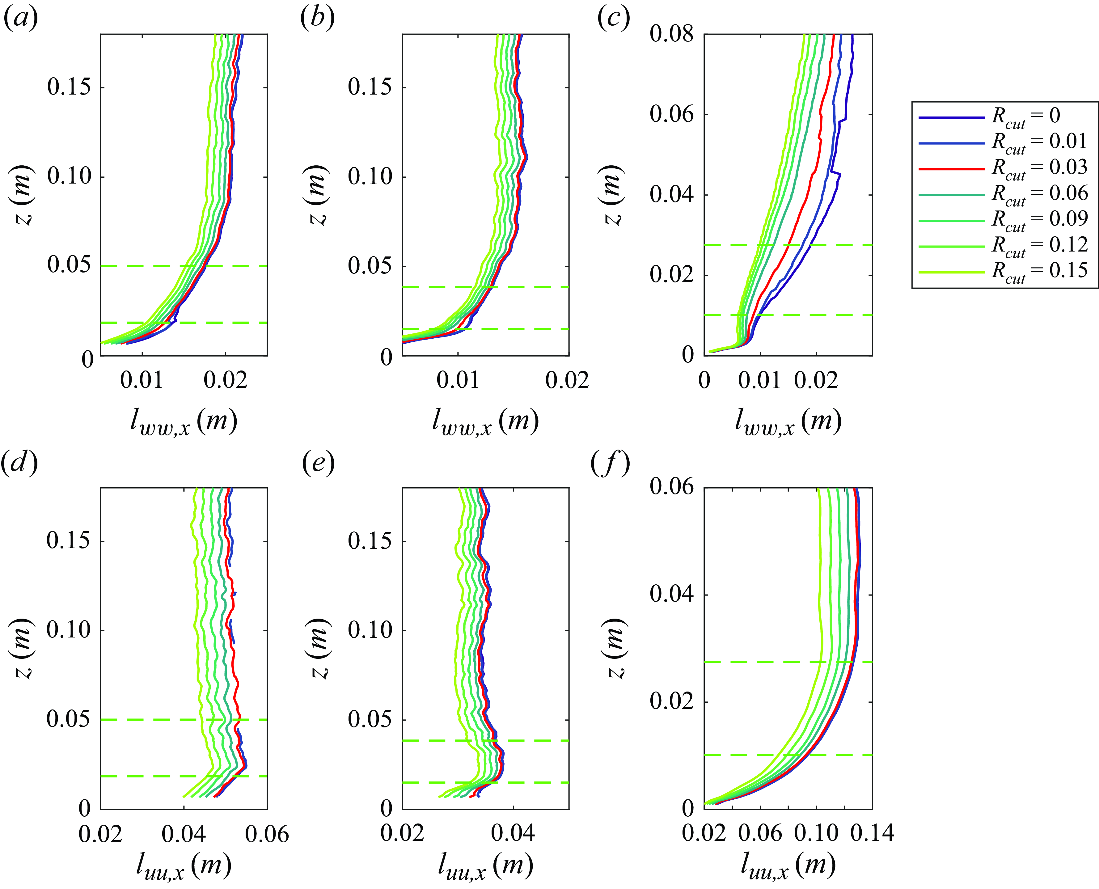
Appendix B. Determination of the Surface-Layer Boundaries
This section describes the process implemented to define the upper and lower bounds of the surface-layer region, $\delta _U$
and
$\delta _U$
and $\delta _L$
respectively, from the linear portion of the
$\delta _L$
respectively, from the linear portion of the $l_{ww,x}(z)$
profile. An iterative procedure is implemented to systematically determine the most linear region of the integral length scale profile and the upper and lower bounds of the surface layer as described below.
$l_{ww,x}(z)$
profile. An iterative procedure is implemented to systematically determine the most linear region of the integral length scale profile and the upper and lower bounds of the surface layer as described below.
-
Step 1 An initial guess of the bounds of linear region are set. For the lower boundary the height of the SAS was used and the second point was selected as a point within the linear region of the plot.
-
Step 2 The line of best fit of the data between these bounds is calculated using least squares linear regression. The resulting linear fit is plotted with the original profile in figure 17(a).
-
Step 3 The relative error between the data and the line of best fit is calculated as
(B1)where \begin{equation} \epsilon = -\frac {l(z) -l_{fit}(z)}{l_{fit}(z)}, \end{equation}
$l(z)$
is the experimentally calculated integral length scale profile and
$l_{fit}(z)$
is the line of best fit calculated in step 2. The resulting relative error is plotted in figure 17(b).
\begin{equation} \epsilon = -\frac {l(z) -l_{fit}(z)}{l_{fit}(z)}, \end{equation}
$l(z)$
is the experimentally calculated integral length scale profile and
$l_{fit}(z)$
is the line of best fit calculated in step 2. The resulting relative error is plotted in figure 17(b).
-
Step 4 New bounds for the linear region are selected at the points where the error becomes greater than 1 %,
$\epsilon \gt 0.01$
. These points are identified in figure 17 with blue circles. Vertical dashed lines indicate 1% error. -
Step 5 Steps 2–4 are repeated until the upper and lower bounds become stationary. The second iteration of the procedure is presented in in figure 17(c).


Surface-layer determination procedure consists of (a) $l_{ww,x}(z)$
profile in black with initial guess boundaries and least squares linear regression in red, (b) normalised error,
$l_{ww,x}(z)$
profile in black with initial guess boundaries and least squares linear regression in red, (b) normalised error, $\epsilon$
, between linear fit and experimental data where the dashed vertical lines indicate ±1 % error where the new boundary points are selected (blue symbols) and (c)
$\epsilon$
, between linear fit and experimental data where the dashed vertical lines indicate ±1 % error where the new boundary points are selected (blue symbols) and (c) $l_{ww,x}(z)$
profile with revised boundaries and least squares linear regression in blue and initial guess of the boundary points shown by the red symbols.
$l_{ww,x}(z)$
profile with revised boundaries and least squares linear regression in blue and initial guess of the boundary points shown by the red symbols.
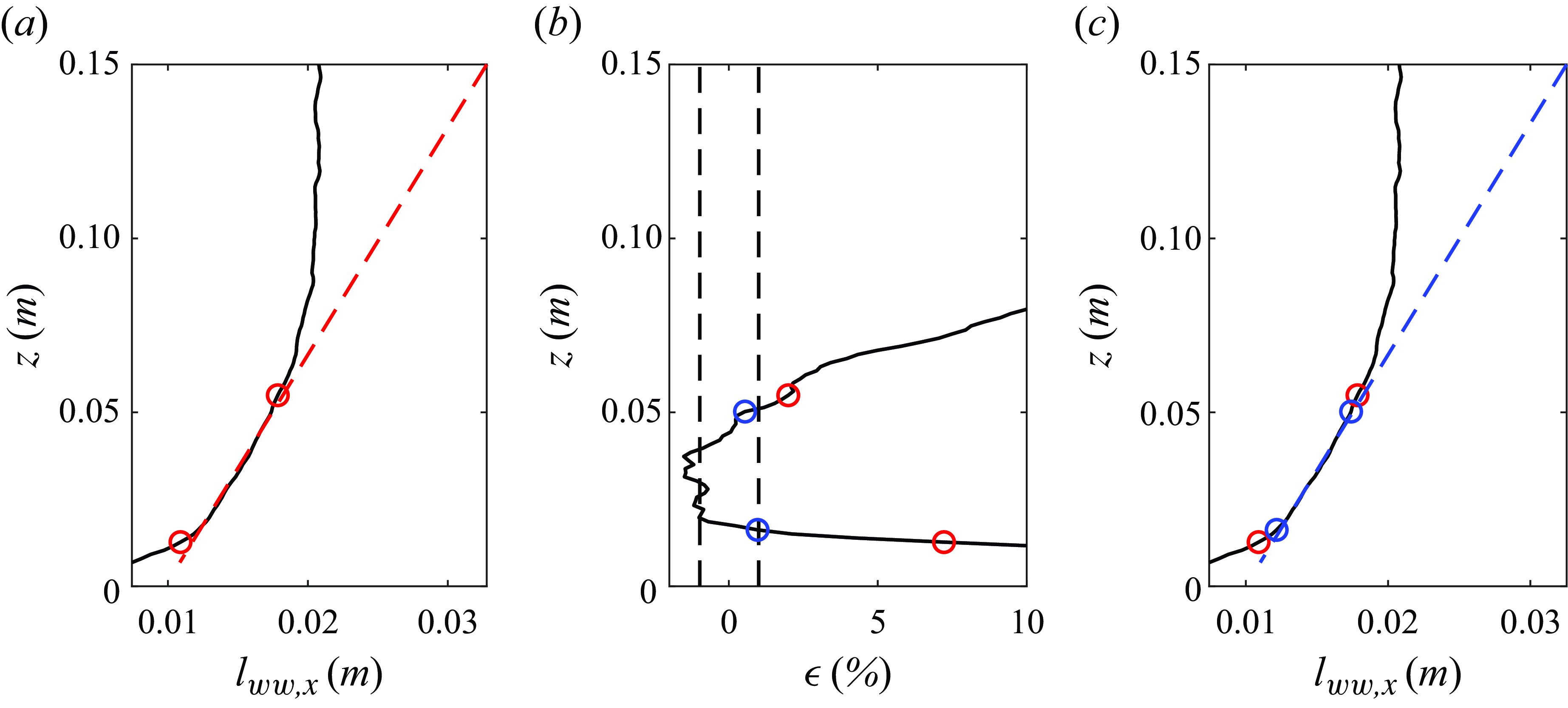


 Open access