Proof. The proof consists in verifying that for $\mu^{\pm}_{M,A}$ -a.e. $(s,x,n)\in\mathbb{R}^{+} \times \mathbb{R}^{d} \times \mathbb{S}^{d-1}$ ,

(3.9) \begin{equation}\int_{s}^{t}g(z,s,x,n) \,{{\mathrm{d}}} z = G(t, \mathbf{e}_{j} \otimes \mathbf {e}_{i}u_{M},s,x,n), \end{equation}

and that the stochastic Fubini theorem can be applied. From (4.33) in Section 4.4 below, we have that for $\mu^{\pm}_{M,A}$ -a.e. $(s,x,n)\in\mathbb{R}^{+}\times\mathbb{R}^{d}\times\mathbb{S}^{d-1}$ with $0<s<t$ and $h_{M}(n)>0$ , it holds that

(3.10) \begin{equation}G(t,\mathbf{e}_{j} \otimes \mathbf{e}_{i}u_{M},s,x,n) = (n\cdot\mathbf{e}_{i}) \mathbf{e}_{j}^{\prime} F(p_{0},x)\mathcal{H}^{d-1}(\mathfrak{D} \cap \mathfrak{H}(h_{M}(n)s/t , n)). \end{equation}

In what follows, we fix such (s, x, n). Using $h_M(n)=\lVert T^{\prime}n\rVert$ , it follows easily that

\[\mathfrak{D}\cap\mathfrak{H}(h_{M}(n)s/t,n)=T(D_{1}\cap\mathfrak{H}(s/t,\upsilon(n))).\]

Since $D_{1}\cap\mathfrak{H}(s/t,\upsilon(n))$ is a $(d-1)$ -dimensional open disk with radius $\sqrt{1-(s/t)^{2}}$ lying in $\mathfrak{H}(s/t,\upsilon(n))$ , it can be parametrised as

\[\varpi(z)=\sqrt{1-(s/t)^{2}}Tz+\dfrac{s}{t}\upsilon(n),\quad z\in\mathbb{S}^{d-1}\cap\upsilon(n)^{\perp}.\]

Furthermore, given that $\mathbb{S}^{d-1}\cap\upsilon(n)^{\perp}$ is a $(d-2)$ -dimensional sphere embedded in $\upsilon(n)^{\perp}$ , we can apply the Area Formula (see e.g. Section 3.3 in [Reference Evans and Gariepy9]) to deduce that

(3.11) \begin{equation}\mathcal{H}^{d-1} (\mathfrak{D}\cap\mathfrak{H}(h_{M}(n)s/t,n)) = \varphi(s/t)\mathcal{H}^{d-1}\big(T\big(D_{1}\cap\upsilon(n)^{\perp}\big)\big). \end{equation}

Equation (3.9) now follows easily from (3.10) and (3.11). Note that the former implies that for all $t>0$ , almost surely

(3.12) \begin{equation}Y_{t}^{\alpha}=\int_{(0,t]\times N(A)}\int_{s}^{t}g(z,s,x,n)\,{{\mathrm{d}}} z\cdot \big[\Lambda_{\alpha}^{+}({{\mathrm{d}}} s\,{{\mathrm{d}}} (x,n))-\Lambda_{\alpha}^{-}({{\mathrm{d}}} s\,{{\mathrm{d}}} (x,n))\big].\end{equation}

Therefore, in order to finish the proof, we need to verify that the stochastic Fubini theorem can be applied for all $1<\alpha<2$ , and for $\alpha=2$ if $d\geq3$ . To do so, we aim to apply Theorem 3.1 in [Reference Barndorff-Nielsen and Basse-O’Connor2]. Such a result, adjusted to our situation, reads as follows. For $1<\alpha\leq2$ , let $\Upsilon$ be a separable one-dimensional strictly $\alpha$ -stable Lévy basis on $\mathcal{S}\subseteq {\mathbb{R}}^K$ with $\sigma$ -finite control measure $\mu$ as described in Section 2.1. In this circumstance, the function $\phi(y,s)$ defined in page 925 in [Reference Barndorff-Nielsen and Basse-O’Connor2] does not depend on s and equals $c_\alpha\rvert y\rvert^\alpha$ , for some constant $c_\alpha>0$ . In particular,

\[\rVert g \rVert_\alpha=\inf\biggl\{w>0\,\colon \int_{\mathcal{S}} \phi (g(q)/w)\mu({{\mathrm{d}}} q)\leq1 \biggr\}=c^{1/\alpha}_{\alpha}\biggl(\int_{\mathcal{S}}\rvert g(q)\rvert^{\alpha}\mu({{\mathrm{d}}} q)\biggr)^{1/\alpha},\]

where g is an arbitrary measurable function. Therefore, according to Theorem 3.1 in [Reference Barndorff-Nielsen and Basse-O’Connor2], if $f\,\colon {\mathbb{R}}^+\times\mathcal{S}\to{\mathbb{R}}$ is a measurable function such that

(3.13) \begin{equation}\begin{split} & \textrm{(i)} \quad \int_{\mathcal{S}}\rvert f(z,q)\rvert^{\alpha}\mu({{\mathrm{d}}} q)<\infty\quad\text{for every $z\geq0$}, \\ & \text{(ii)}\quad \int_0^\infty\biggl(\int_{\mathcal{S}}\rvert f(z,q)\rvert^{\alpha}\mu({{\mathrm{d}}} q)\biggr)^{1/\alpha}\,{{\mathrm{d}}} z<\infty,\end{split}\end{equation}

then

\[\int_0^\infty\biggl[\int_{\mathcal{S}}f(z,q)\Upsilon({{\mathrm{d}}} q)\biggr]\,{{\mathrm{d}}} z=\int_{\mathcal{S}}\biggl[\int_0^\infty f(z,q)\,{{\mathrm{d}}} z\biggr]\Upsilon({{\mathrm{d}}} q),\]

in the sense that both integrals exist and are equal almost surely. Returning to our proof, note that by the Lévy–Khintchine representation, each entry of $\Lambda_{\alpha}^{\pm}$ is a separable one-dimensional strictly $\alpha$ -stable Lévy basis with control measure $\mu^{\pm}_{M,A}$ . As a consequence of this, (2.6), and (3.13), we can swap the order of integration in (3.12) whenever

(3.14) \begin{align} &\int_{(0,z] \times N(A)}\| g(z,s,x,n) \|^{\alpha}\mu^{\pm}_{M,A}({{\mathrm{d}}} s \,{{\mathrm{d}}} (x,n))<\infty \quad \text{for all $ z\geq0$,} \\[-9pt] \nonumber \end{align}

(3.15) \begin{align} &\int_{0}^{t} \biggl(\int_{(0,z] \times N(A)}\| g(z,s,x,n) \|^{\alpha}\mu^{\pm}_{M,A}({{\mathrm{d}}} s \,{{\mathrm{d}}} (x,n)) \biggr)^{1/\alpha} \,{{\mathrm{d}}} z<\infty. \\[9pt] \nonumber \end{align}

This is easily obtained by noting that the integral in (3.14) equals

\[C\times z^{1-\alpha}\int_{0}^{1}|\varphi^{\prime}(y)y|^{\alpha}\,{{\mathrm{d}}} y,\]

where, due to the continuity of F and the compactness of the sphere, the constant C is given by

\[\int_{\partial A}\|(n_{A}(x)\cdot\mathbf{e}_{i})\,\mathbf{e}_{j}^{\prime}F(p_{0},x)\mathcal{H}^{d-1}\big(T\big(D_{1}\cap\upsilon(n_{A}(x))^{\perp}\big)\big)\|^{\alpha}\lVert T^{\prime}n_{A}(x)\rVert\mathcal{H}^{d-1}({{\mathrm{d}}} x)<\infty.\]

Thus (3.14) and (3.15) hold if and only if either $1<\alpha<2$ and $d\geq2$ or $\alpha=2$ and $d\geq 3$ .

Proof. Fix $p_{0}\in\mathbb{R}^{d}$ and put $H(p,q)\,:\!=\, F(p,q)\mathbf{1}_{A}(q-p)$ . From (4.2), it is enough to show that

(4.5) \begin{equation}\| X^{(4)}(p_{0}+r\,t\,y)\| \leq C\xi_{t,r},\end{equation}

for some positive (finite a.s.) random variable $\xi_{t,r}$ , and that for all $\beta\geq0$ ,

(4.6) \begin{equation}m_\beta=\mathbb{E} \big(\| X^{(i)}(p_{0}+r\,t\,y)\| ^{\beta}\big)\leq C,\quad i=1,2,3,\end{equation}

uniformly on $y\in M$ . For simplicity and notational convenience, we set $p_{0}=0$ for the remainder of the proof. Thus, by letting $g(q,x)\,:\!=\, \mathbf{1}_{A_{\oplus rt}}(q)\| x\| \mathbf{1}_{D_{1}^{c}}(x)$ , we see that (4.5) holds if we set

\[\xi_{t,r}\,:\!=\, \int_{A_{\oplus rt}}\int_{\mathbb{R}^{m}}g(q,x)N({{\mathrm{d}}} q\,{{\mathrm{d}}} x),\]

because F is continuous and $A+r\,t\,y\subseteq A\oplus rtM\subseteq A_{\oplus rt}$ . The $\mathbb{P}$ -a.s. finiteness of $\xi_{t,r}$ follows from the fact that $\int1\land\| g\| \,{{\mathrm{d}}} \varrho<\infty$ and Lemma 12.13 in [Reference Kallenberg19]. On the other hand, since F is continuous and A compact, it is clear that (4.6) holds for $i=1,2$ . Now, given that $H(p,\cdot)$ has compact support, $X^{(3)}$ has finite moments of all orders and from Corollary 1.2.6 in [Reference Turner44], for every $\theta\geq2$ ,

\[m_{\theta}\leq C\int_{A+p}\int_{D_{1}}\big(\| F(p_{0}+r\,t\,y,q)x\| ^{2}\lor\| F(p_{0}+r\,t\,y,q)x\| ^{\theta} \big)\nu({{\mathrm{d}}} x)\,{{\mathrm{d}}} q\leq C,\]

once again by the continuity of F. This easily implies that (4.6) is also valid for $i=3$ .

Proof of (4.9). Let

(4.11) \begin{equation}H(p,q)\,:\!=\, F(p,q)\mathbf{1}_{A}(q-p). \end{equation}

The main step consists in showing that the stochastic Fubini theorem can be applied. Suppose for a moment that this is the case. Then, by means of this and (3.3), we have that for every $t\geq 0 $ and $f\in L^{2}(\mathcal{H}^{d-1}\downharpoonright_{M})$ ,

(4.12) \begin{align}Y_{r}(t,f)&=\sum_{j=1}^{m}\sum_{i=1}^{d}\int_{\mathbb{R}^{d}}\int_{M} \big[H^{(i,j)}(r\,t\,y,q)-H^{(i,j)}(0,q) \big]f^{(i)}(y)\mathcal{H}^{d-1}({{\mathrm{d}}} y)L^{(j)}({{\mathrm{d}}} q)\notag \\&=\int_{\mathbb{R}^{d}}\int_{M}f(y)^{\prime}[H(r\,t\,y,q)-H(0,q)]\mathcal{H}^{d-1}({{\mathrm{d}}} y)L({{\mathrm{d}}} q)\quad \text{$\mathbb{P}$-a.s.}\end{align}

Furthermore, we have the following:

1. (i) If $q\in (A\oplus rtM)^c $ , then $\mathbf{1}_A(q-r\,t\,y)=0$ for all $y\in M$ . Indeed, if this were not the case, we would have that $q-r\,t\,y\in A$ , implying that $q=(q-r\,t\,y)+r\,t\,y\in A\oplus rtM$ , which is absurd.

2. (ii) In contrast, by definition, if $q\in (A\ominus rtM) $ , then $\mathbf{1}_A(q-r\,t\,y)=1$ for all $y\in M$ .

All the above observations result in

\begin{align*}\sum_{l=1}^{n}\theta_{l}Y_{r}(t_{l},f)&=\sum_{l=1}^{n}\theta_{l}\int_{A}\int_{M}f(y)^{\prime}[H(rt_{l}y,q)-F(0,q)]\mathcal{H}^{d-1}({{\mathrm{d}}} y)L({{\mathrm{d}}} q)\\&\quad +\sum_{l=1}^{n}\theta_{l}\int_{A^{c}}\int_{M}f(y)^{\prime}H(rt_{l}y,q)\mathcal{H}^{d-1}({{\mathrm{d}}} y)L({{\mathrm{d}}} q)\\&=\sum_{l=1}^{n}\theta_{l}\int_{A\cap(\cap_{k=1}^{n}A\ominus rt_{k}M)}\int_{M}f(y)^{\prime}[F(rt_{l}y,q)-F(0,q)]\mathcal{H}^{d-1}({{\mathrm{d}}} y)L({{\mathrm{d}}} q)\\&\quad +\sum_{l=1}^{n}\theta_{l}\int_{A\cap(\cap_{k=1}^{n}A\ominus rt_{k}M)^{c}}\int_{M}f(y)^{\prime}[H(rt_{l}y,q)-F(0,q)]\mathcal{H}^{d-1}({{\mathrm{d}}} y)L({{\mathrm{d}}} q)\\&\quad +\sum_{l=1}^{n}\theta_{l}\int_{A^{c}\cap(\cup_{k=1}^{n}A\oplus rt_{k}M)}\int_{M}f(y)^{\prime}H(rt_{l}y,q)\mathcal{H}^{d-1}({{\mathrm{d}}} y)L({{\mathrm{d}}} q),\end{align*}

which is exactly (4.9).

To complete our argument, it remains to justify the use of the stochastic Fubini theorem in (4.12). First, by the Lévy–Khintchine representation (2.2) (see Proposition 11.10 in [Reference Sato39]), $L^{(j)}$ , the jth component of L, is a univariate homogeneous Lévy basis with characteristic triplet

\begin{align*}\gamma_{j}&=\gamma^{(j)}+\int_{\mathbb{R}^{m}}x^{(j)} \big(\mathbf{1}_{\rvert x^{(j)}\rvert\leq1}-\mathbf{1}_{\rVert x\rVert\leq1}\big)\nu({{\mathrm{d}}} x)=\gamma^{(j)}+\int_{\rVert x\rVert>1}x^{(j)}\mathbf{1}_{\rvert x^{(j)}\rvert\leq1}\nu({{\mathrm{d}}} x),\\\sigma_{j}^{2}&=\Sigma^{(\,j,\,j)}, \\\eta_{j}(B)&=\int_{\mathbb{R}}\mathbf{1}_{B}(x_{j})\nu({{\mathrm{d}}} x),\quad B\in\mathcal{B}(\mathbb{R}^{m}).\end{align*}

Therefore, by replacing $\int_K, f(\varphi(u),q)$ , and $\rvert D(u)\rvert \,{{\mathrm{d}}} u$ with $\int_M, g^{(j)}(y,q)$ , and $\mathcal{H}^{d-1}({{\mathrm{d}}} y)$ , respectively, in the proof of Lemma 3 in [Reference Sauri41], we conclude that if $g\,\colon {\mathbb{R}}^d\times{\mathbb{R}}^d\to{\mathbb{R}}^m$ is a measurable function satisfying

1. (i) $\displaystyle\int_{M}\biggl[\int_{\mathbb{R}^{d}}\big(\rVert\gamma\rVert\rVert g(y,q)\rVert+\mathrm{trace}(\Sigma)\rVert g(y,q)\rVert^{2}\big)\,{{\mathrm{d}}} q\biggr]\mathcal{H}^{d-1}({{\mathrm{d}}} y)<\infty$ ,

2. (ii) $\displaystyle\int_{M}\biggl[\int_{\mathbb{R}^{d}}\int_{\rVert x\rVert\leq1}\big(\rVert x\rVert\rVert g(y,q)\rVert\land\rVert x\rVert^{2}\rVert g(y,q)\rVert^{2}\big)\nu({{\mathrm{d}}} x)\,{{\mathrm{d}}} q\biggr]\mathcal{H}^{d-1}({{\mathrm{d}}} y)<\infty$ ,

3. (iii) $\displaystyle\int_{\mathbb{R}^{d}}\int_{\rVert x\rVert>1}(\rVert x\rVert\rVert\chi(q)\rVert\land1)\nu({{\mathrm{d}}} x)\,{{\mathrm{d}}} q<\infty$ ,

where $\chi(q)=\int_Mg(y,q)\mathcal{H}^{d-1}({{\mathrm{d}}} y)$ , then the integrals below exist and almost surely

\[\int_M\biggl[\int_{{\mathbb{R}}^d}g(y,q)L({{\mathrm{d}}} q)\biggr]\mathcal{H}^{d-1}({{\mathrm{d}}} y)=\int_{{\mathbb{R}}^d}\biggl[\int_Mg(y,q)\mathcal{H}^{d-1}({{\mathrm{d}}} y)\biggr]L({{\mathrm{d}}} q).\]

Consequently, to ensure the validity of (4.12), we must check that for every $i=1,\ldots,d$ the function $g^{(j)}(y,q)=[H^{(i,j)}(r\,t\,y,q)-H^{(i,j)}(0,q)]f^{(i)}(y)$ satisfies the above three conditions. As demonstrated above, the support of g must lie in the bounded set $M\times (A\cup A\oplus rtM)$ and, in particular, $\chi$ as above vanishes outside of $A\cup A\oplus rtM$ . Furthermore, by the continuity of F, we also have that $\rVert g\rVert\leq C\rVert f\rVert$ on $M\times (A\cup A\oplus rtM)$ . Condition (i) now follows from these observations and the fact that $f\in L^{2}(\mathcal{H}^{d-1}\downharpoonright_{M})$ and $\mathcal{H}^{d-1}(M)<\infty$ . Similarly, we deduce that the inner integral appearing in (ii) is bounded up to a constant by

\[\rVert f(y)\rVert^2\int_{\rVert x\rVert\leq1}\rVert x\rVert^{2}\nu({{\mathrm{d}}} x)\mathrm{Leb}(A\cup A\oplus rtM),\]

while the integral in (iii) equals

\[\int_{A\cup A\oplus rtM}\int_{\rVert x\rVert>1}(\rVert x\rVert\rVert\chi(q)\rVert\land1)\nu({{\mathrm{d}}} x)\,{{\mathrm{d}}} q\leq\nu(\{\rVert x\rVert>1\})\mathrm{Leb}(A\cup A\oplus rtM)<\infty.\]

This completes our proof.

Proof. For $i=1,\ldots,d,j=1,\ldots,m$ , let

\[R_{F}^{(i,j)}(t,q,y)\,:\!=\, \dfrac{1}{r}\big(F^{(i,j)}(r\,t\,y,q)-F^{(i,j)}(0,q)\big)-t\sum_{k=1}^{d}\partial_{k}F^{(i,j)}(0,q)y^{(k)}.\]

By the Mean Value Theorem and the $C^{1}$ property of F, we have that

(4.13) \begin{equation}\biggl|\int_{M}f(y)^{(i)}R_{F}^{(i,j)}(t,q,y)\mathcal{H}^{d-1}({{\mathrm{d}}} y)\biggr|\leq C\int_{M}\| f(y)\| \| y\| \mathcal{H}^{d-1}({{\mathrm{d}}} y)<\infty,\end{equation}

and, as $r\downarrow0$ ,

\[\int_{M}f(y)^{(i)}R_{F}^{(i,j)}(t,q,y)\mathcal{H}^{d-1}({{\mathrm{d}}} y)\rightarrow0,\]

due to the Dominated Convergence Theorem. Applying this to (4.1) implies that, for all $t\in\mathbb{R}$ ,

\[\dfrac{1}{r}\int_{A}\int_{M}f(y)^{\prime}[F(r\,t\,y,q)-F(0,q)]\mathcal{H}^{d-1}({{\mathrm{d}}} y)L({{\mathrm{d}}} q)\overset{\mathbb{P}}{\rightarrow}t\int_{M}f(y)^{\prime}DX(0)y\mathcal{H}^{d-1}({{\mathrm{d}}} y).\]

Hence it is left to show that, for all $t\in\mathbb{R}$ ,

\[\int_{A\backslash(\cap_{k=0}^{n}A\ominus rt_{k}M)}\int_{M}f(y)^{\prime}\biggl[\dfrac{F(r\,t\,y,q)-F(0,q)}{r}\biggr]\mathcal{H}^{d-1}({{\mathrm{d}}} y)L({{\mathrm{d}}} q)\overset{\mathbb{P}}{\rightarrow}0.\]

This is easily obtained by noticing that, by virtue of (4.1), the characteristic exponent of the latter integral equals

\[\int_{A\backslash(\cap_{k=0}^{n}A\ominus rt_{k}M)}\psi\biggl[z\int_{M}f(y)^{\prime}\biggl[\dfrac{F(r\,t\,y,q)-F(0,q)}{r}\biggr]\mathcal{H}^{d-1}({{\mathrm{d}}} y)\biggr]\,{{\mathrm{d}}} q,\quad z\in\mathbb{R},\]

and, due to (4.13) and the continuity of $\psi$ , it is bounded up to a constant by

\[\sum_{k=1}^{n}\mathrm{Leb}(A\backslash A\ominus rt_{k}M)\rightarrow0\quad \text{as $r\downarrow0$,}\]

thanks to Theorem 1 in [Reference Kiderlen and Rataj20].

Proof of Theorem 3.1.First, recall from our discussion above (see (4.8)) that we only need to concentrate on the case when $\phi(x)=x$ . Furthermore, from (4.9), the above theorem and our assumptions,

\begin{equation*}\dfrac{1}{r^{1/\alpha}}\sum_{l=1}^{n}\theta_{l}Y^{r}(t_{l},f) =\dfrac{1}{r^{1/\alpha}}\Phi_{r}(\mathbf{T},f)+\dfrac{1}{r^{1/\alpha}}\Xi_{r}(\mathbf{T},f)+\mathrm{o}_{\mathbb{P}}(1), \end{equation*}

for every $1<\alpha\leq2$ . Hence it is enough to study the limit behaviour of the functionals $\Xi_{r}(\mathbf{T},f)$ and $\Phi_{r}(\mathbf{T},f)$ defined in (4.10). More specifically, we will show that under our assumptions it holds that

(4.14) \begin{equation}\dfrac{1}{r^{1/\alpha}}\Phi_{r}(\mathbf{T},f) \overset{\mathcal{F}\text{-}d}{\rightarrow}\sum_{l=1}^{n}\theta_{l}Y^{\alpha,+}(t_{l},f),\quad\dfrac{1}{r^{1/\alpha}}\Xi_{r}(\mathbf{T},f)\overset{\mathcal{F}\text{-}d}{\rightarrow}\sum_{l=1}^{n}\theta_{l}Y^{\alpha,-}(t_{l},f),\end{equation}

where (recall the definition of $\Lambda_{\alpha}^{\pm}$ introduced in Section 3.1)

\[Y^{\alpha,\pm}(t,f)\,:\!=\, \pm\int_{(0,t]\times N(A)}G(t,f,s,x,n)\cdot\Lambda_{\alpha}^{\pm}({{\mathrm{d}}} s\,{{\mathrm{d}}} (x,n)),\quad 1<\alpha\leq2,\]

The proof will then be completed by observing that:

1. (i) $\Xi_{r}(\mathbf{T},f)$ and $\Phi_{r}(\mathbf{T},f)$ are independent,

2. (ii) $Y^{\alpha}=Y^{\alpha,+}+Y^{\alpha,-}$ .

For the rest of the proof we restrict our attention to $\Xi_{r}(\mathbf{T},f)$ since the arguments used in this case can be easily extrapolated to $\Phi_{r}(\mathbf{T},f)$ . Let us now verify that (4.14) is satisfied if Assumption ${\mathbf{A}}_\alpha$ holds for some $1<\alpha\leq2$ and A is a compact gentle set. Let $\mathcal{F}_L\,:\!=\, \sigma\{L(B)\,\colon B\in \mathcal{B}^{\mathrm{Leb}}_{b}(\mathbb{R}^{d})\}$ . Since $\Xi_{r}(\mathbf{T},f)$ is $\mathcal{F}_L$ -measurable, and thanks to Proposition 3.5 in [Reference Häusler and Luschgy13], it is sufficient to check that the convergence in (4.14) holds only weakly. To see that this is the case, fix $r_0>0$ , and observe that for any $r\leq r_0$

\begin{align*} \dfrac{\Xi_{r_0}(\mathbf{T},f)}{r_0^{1/\alpha}}&=r_0^{-1/\alpha}\int_{\mathbf{B}_{r_0}\setminus\mathbf{B}_{r}}\sum_{l=1}^{n}\theta_{l}k_{l}^{(2)}(r_0,q)L({{\mathrm{d}}} q)+r_0^{-1/\alpha}\int_{\mathbf{B}_{r_0}\cap\mathbf{B}_{r}} \sum_{l=1}^{n}\theta_{l}k_{l}^{(2)}(r_0,q)L({{\mathrm{d}}} q)\\& \,=\!:\, \tilde{\Xi}_{0}^{r,1}+\tilde{\Xi}_{0}^{r,2},\end{align*}

where $\mathbf{B}_r=A\backslash(\cap_{k=1}^{n}A\ominus rt_{k}M)$ . By construction, $\tilde{\Xi}_{0}^{r,1}$ is independent of $ \Xi_{r}(\mathbf{T},f)$ and $\tilde{\Xi}_{0}^{r,2}$ for every $r\leq r_0$ . Furthermore, given that

\[\mathrm{Leb}(\mathbf{B}_r\cap\mathbf{B}_{r_0})\leq\sum_{k=1}^{n}\mathrm{Leb}(A\backslash A\ominus rt_{k}M)\rightarrow0\quad \text{as $r\downarrow0$,}\]

and F is continuous, we also have that $\tilde{\Xi}_{0}^{r,2}\overset{\mathbb{P}}{\rightarrow}0$ and $\tilde{\Xi}_{0}^{r,1}\overset{\mathbb{P}}{\rightarrow}\Xi_{r_0}(\mathbf{T},f)$ . Hence, if (4.14) holds only weakly, the above properties, along with Slutsky’s theorem, yield

\[ \biggl(\dfrac{\Xi_{r}(\mathbf{T},f)}{r^{1/\alpha}},\dfrac{\Xi_{r_0}(\mathbf{T},f)}{r_0^{1/\alpha}}\biggr)\overset{d}{\rightarrow}\Biggl(\sum_{l=1}^{n}\theta_{l}Y^{\alpha,+}(t_{l},f),\dfrac{\Xi_{r_0}(\mathbf{T},f)}{r_0^{1/\alpha}}\Biggr),\]

which, according to part (iii) of Exercise 3.9 in [Reference Häusler and Luschgy13], results in the sought-after $\mathcal{F}$ -stable convergence.

Let $\psi_{\alpha}$ be as in (2.4) but with $\lambda$ replaced by $\bar{\lambda}({{\mathrm{d}}} u)=\alpha K(u)\lambda({{\mathrm{d}}} u)$ when $1<\alpha<2$ ; otherwise we set $\psi_{\alpha}(w)=-\tfrac{1}{2}w^{\prime}\Sigma w $ . From Lemma 4.3 and Remark 4.2 below, for all $z\in\mathbb{R}$ , it holds that

(4.15) \begin{equation}\mathcal{C}\biggl(z\ddagger\dfrac{1}{r^{1/\alpha}}\Xi_{r}(\mathbf{T},f)\biggr)=\dfrac{1}{r}\int_{A\backslash(\cap_{k=1}^{n}A\ominus rt_{k}M)}\psi_{\alpha}\big(zI_{\mathbf{T},f}^{r}(q)\big)\,{{\mathrm{d}}} q+\mathrm{o}(1),\end{equation}

where

(4.16) \begin{equation}I_{\mathbf{T},f}^{r}(q)\,:\!=\, \sum_{l=1}^{n}\theta_{l}\int_{M}f(y)^{\prime}[H(rt_{l}y,q)-F(0,q)]\mathcal{H}^{d-1}({{\mathrm{d}}} y).\end{equation}

Now set (see Section 2) $u\equiv n_{A}(x)$ , $\delta_{+}=\delta(x,u)$ , and $\delta_{-}=\delta(x,-u)$ . By the continuity of F and $\psi_{\alpha}$ , $\psi_{\alpha}(zI_{\mathbf{T},f}^{r}({\cdot}))$ is locally bounded. Therefore we can apply Proposition 4 (Steiner’s formula for gentle sets) along with the arguments of Theorem 1 in [Reference Kiderlen and Rataj20] (cf. [Reference Hug, Last and Weil15]) to conclude that

\[\dfrac{1}{r}\int_{A\backslash(\cap_{k=1}^{n}A\ominus rt_{k}M)}\psi_{\alpha}\bigl(zI_{\mathbf{T},f}^{r}(q)\bigr)\,{{\mathrm{d}}} q=\dfrac{1}{r}\int_{\partial A}g_{r}(x,z)\mathcal{H}^{d-1}({{\mathrm{d}}} x)+\mathrm{o}(1),\]

in which we have let

\[g_{r}(x,z)\,:\!=\, \int_{-\delta_{-}}^{0}\psi_{\alpha}\bigl(zI_{\mathbf{T},f}^{r}(x+su)\bigr)\mathbf{1}_{(\cap_{k=1}^{n}A\ominus rt_{k}M)^{c}}(x+su)\,{{\mathrm{d}}} s.\]

Next we focus on showing that for ${\mathcal H}^{d-1}$ -a.e. $x\in\partial A$ ,

(4.17) \begin{equation}\dfrac{1}{r}g_{r}(x,z)\rightarrow\int_{0}^{t_{n}}\psi_{\alpha}\Biggl({-}z\sum_{l=1}^{n}\theta_{l}G(t_{l},f,s,x,-u)\Biggr)\,{{\mathrm{d}}} sh_{M}({-}u)^{+},\quad r\downarrow0.\end{equation}

To do this, we first note that since A is gentle, for ${\mathcal H}^{d-1}$ -a.e. $x\in\partial A$ , $\delta_{+},\delta_{-}>0$ and

(4.18) \begin{equation}{B}_{+}\,:\!=\, {B}_{\delta_{+}}(x+\delta_{+}u)\subset A^{c},\quad B_{-}\,:\!=\, B_{\delta_{-}}(x-\delta_{-}u)\subseteq A,\end{equation}

where $B_{R}(p)$ is a ball of radius $R>0$ and centre p. Using this and the relation $(A\ominus rtM)^{c}=A^{c}\oplus rtM$ , we deduce that for every $t>0$ it holds that

(4.19) \begin{equation}\mathbf{1}_{(A\ominus rtM)^{c}}(q)=\begin{cases}1 & \text{if $ q\in{B}_{+}+rtp$,}\\0 & \text{if $ q-rtM\subseteq B_{-}$,}\end{cases}\end{equation}

for some $p\in M$ . Fix $x\in\partial A$ satisfying (4.18) and choose $p_{-}(x)\in M$ such that $-p_{-}\cdot u=h_{M}({-}u)$ . From (4.19), we infer that for r small enough and $\delta_{+}>s>-\delta_{-}$ ,

(4.20) \begin{equation}\mathbf{1}_{(\cap_{k=1}^{n}A\ominus rt_{k}M)^{c}}(q)=\begin{cases}1 & \text{if $ s>\mathrm{o}_{+}(rt_{n})-rt_{n}h_{M}({-}u)$,}\\0 & \text{if $ s<-\max_{k} \{rt_{k}h_{M} ({-}u) + \mathrm{o}_{-} (rt_{k})$}\},\end{cases}\end{equation}

where $q=x+su$ and $\mathrm{o}_{\pm}(r)=(\delta_{\pm}-\sqrt{\delta_{\pm}^{2}-r^{2}})=\mathrm{o}(r)$ . Hence

(4.21) \begin{align}\dfrac{1}{r}g_{r}(x,z)= & \int_{-t_{n}h_{M}({-}u)}^{0}\psi_{\alpha}\big(zI_{\mathbf{T},f}^{r}(x+rsu)\big)\,{{\mathrm{d}}} s\mathbf{1}_{h_{M}({-}u)>0}+\mathrm{o}(1),\end{align}

where we further used that $\psi_{\alpha}(zI_{\mathbf{T},f}^{r}({\cdot}))$ is locally bounded and made a change of variables. Let us now compute the limit of $I_{\mathbf{T},f}^{r}(x+rsu)$ . To do this, thanks to Theorem 10.10 in [Reference Mattila25], we may and do assume that

(4.22) \begin{equation}\mathcal{H}^{d-1}(M\cap\{y\,\colon ty\cdot u=s\})=0.\end{equation}

Reasoning as in (4.19) and (4.20), we conclude that, for all $t\geq0$ and $q_{r}(t)=x+sru-r\,t\,y$ ,

\[\mathbf{1}_{A}(q_{r}(t))=\begin{cases}1 & \text{if $ ty\cdot u > s+\mathrm{o}_{-}(tr)/r$,}\\0 & \text{if $ ty\cdot u < s-\mathrm{o}_{+}(tr)/r$.}\end{cases}\]

Thus

\begin{align*}I_{\mathbf{T},f}^{r}(q)& =- \sum_{l=1}^{n}\theta_{l}\int_{M}f(y)^{\prime}\mathbf{1}_{t_{l}y\cdot u < s-\mathrm{o}_{+}(rt_{l})/r}\mathcal{H}^{d-1}({{\mathrm{d}}} y)F(0,q_{r}(t_l))+\mathrm{o}(1)\\& \rightarrow -\sum_{l=1}^{n}\theta_{l}\int_{M}f(y)^{\prime}\mathbf{1}_{({-}\infty,s]}(t_{l}y\cdot u)\mathcal{H}^{d-1}({{\mathrm{d}}} y)F(0,x),\end{align*}

where we also used (4.22) and the fact that ${\mathrm{o}_{\pm}(r)}{r} \downarrow0$ as $r \downarrow0$ . The convergence in (4.17) follows now by applying this to (4.21) and a simple change of variables. Finally, since

\[| g_{r}(x,z)|\leq C\sum_{k=1}^{n}\int_{-\delta_{+}}^{0}\mathbf{1}_{A_{\oplus rt_{k}}^{*}}(x+sn_{A}(x))\,{{\mathrm{d}}} s\leq Cr,\]

the limits in (4.14) can now be easily obtained by the Dominated Convergence Theorem, (4.17), and the fact that $\mathbf{1}_{[sh_{M}(u),+\infty)}(ty\cdot u)=0$ for $s>t.$

Proof of Theorem 3.2.Observe first that in this situation

\begin{align*} \dfrac{1}{r}\sum_{l=1}^{n}\theta_{l}Y^{r}(t_{l},f)= & \sum_{l=1}^{n}\theta_{l}t_{l}\int_{M}f(y)^{\prime}\nabla X(p_{0})y\mathcal{H}^{d-1}({{\mathrm{d}}} y)+\mathrm{o}_{\mathbb{P}}(1)\notag \\& +\dfrac{1}{r}\Psi_{r}(\mathbf{T},f)+\dfrac{1}{r}\Xi_{r}(\mathbf{T},f),\end{align*}

due to Theorem 4.1. Note also that thanks to Lemma 4.3, (4.15) also holds if we replace $\psi_{\alpha}$ with $\tilde{\psi}(w)=\mathbf{i}\gamma_{0}\cdot w$ . Therefore, by setting

\[Y^{1,\pm}(t,f)\,:\!=\, \pm\int_{(0,t]\times N(A)}G(t,f,s,x,n)\cdot\gamma_{0}\mu^{\pm}_{M,A}({{\mathrm{d}}} s\,{{\mathrm{d}}} (x,n)),\]

and arguing exactly as in the proof of Theorem 3.1, we deduce that

\[ \dfrac{1}{r}\Xi_{r}(\mathbf{T},f)\overset{\mathbb{P}}{\rightarrow} \sum_{l=1}^{n} \theta_{l}Y^{1,-}(t_{l},f).\]

Similarly, we obtain

\[ \dfrac{1}{r}\Psi_{r}(\mathbf{T},f)\overset{\mathbb{P}}{\rightarrow} \sum_{l=1}^{n} \theta_{l}Y^{1,+}(t_{l},f).\]

Therefore, in order to finish the proof, we only need to check that the sum of $Y^{1,+}(t,f)$ and $Y^{1,-}(t,f)$ equals

\[t\sum_{i,k,m} \int_{M}\int_{A+p_{0}}f(y)^{(i)} \partial_{k+d}F^{(i,j)} (p_{0},x) \gamma_{0}^{(i)}y^{(k)} \,{{\mathrm{d}}} q \mathcal{H}^{d-1}({{\mathrm{d}}} y).\]

This relation is obtained easily by applying Fubini’s theorem, using the identity

\[\int_{0}^{t}G(t,f,s,x,\pm u)\,{{\mathrm{d}}} s=\dfrac{t}{h_{M}(u)}\int_{M}f(y)^{\prime}(\pm y\cdot u)^{+}\mathcal{H}^{d-1}({{\mathrm{d}}} y)F(p_{0},x),\quad h_{M}(\pm u)>0,\]

and by the classical Divergence Theorem.

Proof. By the Lévy–Khintchine representation, $\Upsilon^{(j)}$ , the jth component of $\Upsilon$ , is a univariate homogeneous Lévy basis with Lévy measure

\[\eta_{j}(A)=\int_{{\mathbb{R}}^m}\mathbf{1}_{A}(x_j)\nu({{\mathrm{d}}} x).\]

Thus, if $F\,\colon {\mathbb{R}}^d\rightarrow{\mathbb{R}}^{d\times m}$ is bounded with compact support, Proposition 2.6 and Theorem 2.7 in [Reference Rajput and Rosiński33] imply that the ID random variable $Y^{(i,j)}=\int_{{\mathbb{R}}^d}F^{(i,j)}(q)\Upsilon^{(j)}({{\mathrm{d}}} q)$ is centred, does not have Gaussian component, and its Lévy measure is given by

\[\lambda_j(B)=\int_{\mathbb{R}^d}\int_{{\mathbb{R}}^m}\mathbf{1}_{B}\big(x_jF^{(i,j)}(q)\big)\nu({{\mathrm{d}}} x)\,{{\mathrm{d}}} q.\]

Our assumptions now yield that for some $p\geq2$ ,

\[\int_{{\mathbb{R}}}\rvert y\rvert^p\mathbf{1}_{\rvert y\rvert>1}\lambda_j({{\mathrm{d}}} y)\leq \int_{\mathbb{R}^d}\int_{{\mathbb{R}}^m}\rVert x\rVert^p \big\rvert F^{(i,j)}(q)\big\rvert^p\nu({{\mathrm{d}}} x)\,{{\mathrm{d}}} q<\infty.\]

Thus, according to Theorem 25.3 in [Reference Sato40] and Corollary 1.2.7 in [Reference Turner44], we have ${\mathbb{E}}(\rvert Y^{(i,j)}\rvert^p)<\infty$ and

\[{\mathbb{E}}\big(\rvert Y^{(i,j)}\rvert^p \big)\leq C_p\max\bigl\{\big(K^{(i,j)}_p \big)^{p/2},K^{(i,j)}_p\bigr\},\]

where

\[K^{(i,j)}_p=\int_{\mathbb{R}^d}\int_{{\mathbb{R}}^m}\big(\big\rvert x_jF^{(i,j)}(q)\big\rvert^2 \vee \big\rvert x_jF^{(i,j)}(q)\big\rvert^p \big)\nu({{\mathrm{d}}} x)\,{{\mathrm{d}}} q.\]

Using $\tfrac{1}{2}(x+y)\leq\max\{x,y\}\leq x+y$ for $x,y\geq0$ and the fact that $\int_{{\mathbb{R}}^m}\rVert x\rVert^p\nu({{\mathrm{d}}} x)<\infty$ , we further obtain

\[K^{(i,j)}_p\leq C_{p,\nu}\max \big\{(\kappa_p)^{p/2},\kappa_p \big\}.\]

The estimate in (4.24) now follows from this inequality and the definition of $\int_{{\mathbb{R}}^d}F(q)\Upsilon({{\mathrm{d}}} q)$ .

Proof of Lemma 4.1.Without loss of generality, we may and do assume that $0 < r\leq r_0$ for some fixed $r_0>0$ . By the Mean Value Theorem, for all $\phi\in C_{\beta}^{2}$ , it holds that

\[\| \phi(x)-\phi(y)-D\phi(y)(x-y)\| \leq C \big(1+\| y\| ^{\beta-2} \big)\big(\lVert x-y\| ^{2}\lor\| x-y\| ^{\beta} \big),\,x,y\in\mathbb{R}^{d}.\]

As a result of this, the norm of

\[\phi(X(p_{0}+r\,t\,y))-\phi(X(p_{0}))-D\phi(X(p_{0}))[X(p_{0}+r\,t\,y)-X(p_{0})]\]

is bounded up to a random constant (that only depends on $X(p_0)$ ) by

\[\| X(p_{0}+r\,t\,y)-X(p_{0})\| ^{2}\lor\| X(p_{0}+r\,t\,y)-X(p_{0})\| ^{\beta}.\]

In consequence, it is enough to show that, for all $i=1,2,3,4$ (remember the decomposition (4.2)), as $r\downarrow0$ ,

(4.25) \begin{equation}\dfrac{1}{r^{1/\alpha}}\int_{M}\| f(y)\| \big\| X^{(i)}(p_{0}+r\,t\,y)-X^{(i)}(p_{0}) \big\| ^{\beta_{0}}\mathcal{H}^{d-1}({{\mathrm{d}}} y)\overset{\mathbb{P}}{\rightarrow}0, \quad \beta_{0}\,:\!=\, 2\lor\beta.\end{equation}

For simplicity and notational convenience, we set $p_{0}=0$ for the remainder of the proof. Now, for $i=1,\ldots,4$ , we write

(4.26) \begin{align}X^{(i)}(r\,t\,y)-X^{(i)}(0) & =\int_{A\cap A\ominus\{r\,t\,y\}}(F(r\,t\,y,q)-F(0,q))L_{i}({{\mathrm{d}}} q)\notag \\&\quad +\int_{A\oplus\{r\,t\,y\}\backslash A}F(r\,t\,y,q)L_{i}({{\mathrm{d}}} q)\notag \\&\quad +\int_{A\backslash A\ominus\{r\,t\,y\}}(H(r\,t\,y,q)-F(0,q))L_{i}({{\mathrm{d}}} q)\end{align}

where $L_{i}$ is the Lévy basis associated to $X^{(i)}$ via (4.2) and H as in (4.11). Using the fact that $A\oplus rtM\subseteq A_{\oplus rt}$ and $(A\ominus rtM)^{c}\subseteq A^{c}\oplus rtD_{1}$ , as well as the $C^{1}$ property of F, we deduce that for any $l\geq1$ there is a constant $C>0$ depending only on $F,A,M,r_0$ , and t, such that

(4.27) \begin{equation} \begin{aligned}\int_{A\cap A\ominus\{r\,t\,y\}}\rVert F(r\,t\,y,q)-F(0,q)\rVert^l\,{{\mathrm{d}}} q & \leq Cr^l,\\\int_{A\oplus\{r\,t\,y\}\backslash A}\rVert F(r\,t\,y,q)\rVert^l\,{{\mathrm{d}}} q&\leq C \mathrm{Leb}(A_{\oplus rt}\backslash A),\\\int_{A\backslash A\ominus\{r\,t\,y\}}\rVert H(r\,t\,y,q)-F(0,q)\rVert^l\,{{\mathrm{d}}} q& \leq C\mathrm{Leb}(A\backslash A\ominus rtD_{1}).\end{aligned} \end{equation}

This immediately gives

\[ \big\| X^{(1)}(r\,t\,y)-X^{(1)}(0)\big\| \leq C(r+\mathrm{Leb}(A_{\oplus rt}\backslash A)+\mathrm{Leb}(A\backslash A\ominus rtD_{1})).\]

Now, since $L_{2}$ is a purely Gaussian homogeneous Lévy measure, the discussion in Remark 4.1 along with (4.27) asserts that

\[\mathbb{E}\big( \big\| X^{(2)}(r\,t\,y)-X^{(2)}(0)\big\| ^{\beta_{0}}\big)\leq C\big(r^{2}+\mathrm{Leb}(A_{\oplus rt}\backslash A)+\mathrm{Leb}(A\backslash A\ominus rtD_{1})\big){}^{\beta_{0}/2}.\]

Continuing with the case $i=3$ , note first that by construction, $L_3$ has characteristic triplet $(0, 0, \nu\downharpoonright_{D_{1}}) $ , with $\nu\downharpoonright_{D_{1}}$ denoting the restriction of $\nu$ to the unit disk $D_1$ . As a result, Lemma 4.1 applies to each of the stochastic integrals appearing in the decomposition (4.26). Utilising this and (4.27), we deduce that for r small enough,

\[\mathbb{E} \big(\| X^{(3)}(r\,t\,y)-X^{(3)}(0)\| ^{\beta_{0}}\big)\leq C(r^{\beta_{0}}+\mathrm{Leb}(A_{\oplus rt}\backslash A)+\mathrm{Leb}(A\backslash A\ominus rtD_{1})).\]

An application of the above estimates and Theorem 1 in [Reference Kiderlen and Rataj20] shows that (4.25) is valid for $i=1,2,3$ . On the other hand, using (4.3), (4.26), the $C^1$ property of F, and arguing as in the proof of Proposition 3.1, we infer that uniformly on $y\in M$ , $\mathbb{P}$ -a.s.

(4.28) \begin{equation}\big\| X^{(4)}(r\,t\,y)-X^{(4)}(0)\big\| ^{\beta_{0}} \leq C(r\chi+\xi_{r})^{\beta_{0}},\end{equation}

where

\[\chi\,:\!=\, \int_{A}\int_{\mathbb{R}^{m}}\| x\| \mathbf{1}_{D_{1}^{c}}(x)N({{\mathrm{d}}} q\,{{\mathrm{d}}} x)\]

and

\[\xi_{r}\,:\!=\, \int_{(A_{\oplus rt}\backslash A)\cup(A\backslash A\ominus rtD_{1})}\int_{\mathbb{R}^{m}}\| x\| \mathbf{1}_{D_{1}^{c}}(x)N({{\mathrm{d}}} q\,{{\mathrm{d}}} x).\]

Therefore, in order to see that (4.25) is also satisfied for $i=4$ , we only need to check that

(4.29) \begin{equation}r^{-1/\alpha\beta_{0}}\xi_{r}\overset{\mathbb{P}}{\rightarrow}0.\end{equation}

The above relation is easily obtained by noting that $r^{-1/\alpha\beta_{0}}\xi_{r}$ is infinitely divisible with characteristic exponent

\[\mathrm{Leb}((A_{\oplus rt}\backslash A)\cup(A\backslash A\ominus rtD_{1}))\int_{\| x\| >1}\bigl({{\mathrm{e}}}^{\mathbf{i}zr^{-1/\alpha\beta_{0}}\| x\| }-1\bigr)\nu({{\mathrm{d}}} x),\quad z\in\mathbb{R},\]

which is bounded up to a constant by r, once again, due to Theorem 1 in [Reference Kiderlen and Rataj20].

Now suppose that $\Sigma=0$ and $\int_{\mathbb{R}^{m}}(1\land\| x\| )\nu({{\mathrm{d}}} x)<\infty$ , in such a way that (4.4) takes the form

\[X(p)=\tilde{X}^{(1)}(p)+X^{(5)}(p)=\int_{A+p}F(p,q)\gamma_{0}\,{{\mathrm{d}}} q+\int_{\mathbb{R}^{d}}\int_{\mathbb{R}^{m}}H(p,q)xN({{\mathrm{d}}} q\,{{\mathrm{d}}} x).\]

Exactly as above, we deduce that

\[\dfrac{1}{r}\int_{M}\| f(y)\| \big\| \tilde{X}^{(1)}(r\,t\,y)-\tilde{X}^{(1)}(0)\big\| ^{\beta_{0}}\mathcal{H}^{d-1}({{\mathrm{d}}} y)\rightarrow0.\]

Moreover, (4.28) remains valid for $X^{(5)}$ if we replace $\mathbf{1}_{D_{1}^{c}}$ with 1 in the definition of $\chi$ and $\xi_{r}$ . Therefore, in order to finish the proof, we need to verify that (4.29) holds for $\alpha=1$ under this new definition of $\xi_{r}$ . To see that this is the case, first note that the characteristic exponent $r^{-1/\beta_{0}}\xi_{r}$ now equals

\[\mathrm{Leb}((A_{\oplus rt}\backslash A)\cup(A\backslash A\ominus rtD_{1}))\int_{\mathbb{R}^{m}}\bigl({{\mathrm{e}}}^{\mathbf{i}zr^{-1/\beta_{0}}\| x\| }-1\bigr)\nu({{\mathrm{d}}} x).\]

Again invoking Theorem 1 in [Reference Kiderlen and Rataj20], we infer that the above quantity is bounded up to a constant by

\[r\int_{\mathbb{R}^{m}}\big(1\land r^{-1/\beta_{0}}\| zx\| \big)\nu({{\mathrm{d}}} x)\leq Cr\big(1\lor r^{-1/\beta_{0}}| z|\big)\rightarrow0\quad \text{as $r\downarrow0$,}\]

because $\beta_{0}\geq2$ . This concludes the proof.

Proof. We will only concentrate on the case where Assumption ${\mathbf{A}}_\alpha$ is satisfied for some $1<\alpha<2$ (the other cases are well known). In this situation, we can write, for $\tau(x)=\mathbf{1}_{\| x\| \leq1}+(1/\| x\| )\mathbf{1}_{\| x\| >1}$ ,

\[r\psi\big(r^{-1/\alpha}w \big)=\mathbf{i}\gamma_{r}\cdot w+\int_{\mathbb{R}^{m}\backslash\{0\}}\big({{\mathrm{e}}}^{\mathbf{i}w\cdot x}-1-\mathbf{i}w\cdot x\tau(x)\big)\nu_{r}({{\mathrm{d}}} x),\]

where

\[\gamma_{r}=r^{1-1/\alpha}\gamma+\int_{1<\|x\|\leq r^{-1/\alpha}}\dfrac{x}{\|x\|}(1-\|x\|)\nu_{r}({{\mathrm{d}}} x)+\int_{\|x\|>r^{-1/\alpha}}\dfrac{x}{\|x\|}\nu_{r}({{\mathrm{d}}} x), \]

and $\nu_{r}({{\mathrm{d}}} x) = r\nu(r^{1/\alpha}\,{{\mathrm{d}}} x)$ . According to Theorem 8.7 in [Reference Sato39], we are left to check that

(4.30) \begin{align}\int_{\mathbb{R}^{m}}f(x)\nu_{r}({{\mathrm{d}}} x) & =r\int_{\mathbb{S}^{m-1}}\int_{0}^{\infty}f\big(r^{-1/\alpha}su\big)\rho_{u}({{\mathrm{d}}} s)\lambda({{\mathrm{d}}} u)\notag \\& \rightarrow\int_{\mathbb{S}^{m-1}}\int_{0}^{\infty}f(su)\dfrac{{{\mathrm{d}}} s}{s^{1+\alpha}}\bar{\lambda}({{\mathrm{d}}} u),\end{align}

for every continuous and bounded function f vanishing on a neighbourhood of $0\in\mathbb{R}^{m}$ , and that

(4.31) \begin{equation}\gamma_{r}\rightarrow\dfrac{\int_{\mathbb{S}^{m-1}}u\bar{\lambda}({{\mathrm{d}}} u)}{(1-\alpha)},\quad \lim_{\epsilon\downarrow0}\limsup_{r\downarrow0}\int_{\|x\|\leq\epsilon}(z\cdot x)^{2}\nu_{r}({{\mathrm{d}}} x)=0.\end{equation}

Set $\rho_{u,r}({{\mathrm{d}}} s)\,:\!=\, r\rho_{u}(r^{1/\alpha}\,{{\mathrm{d}}} s)$ and let $\zeta_{r,u}$ be a sequence of one-dimensional ID distributions with characteristic triplet $(0,0,\rho_{u,r})$ . Equation (3.4) and Theorem 2 in [Reference Ivanovs17] imply that $\zeta_{r,u}$ converges to a one-dimensional strictly $\alpha$ -stable random variable with Lévy measure

\[\alpha K(u)\frac{{{\mathrm{d}}} s}{s^{1+\alpha}}\mathbf{1}_{s>0}.\]

Hence, for any function $g\,\colon \mathbb{R}\rightarrow\mathbb{R}$ continuous and bounded vanishing on a neighbourhood of $0\in\mathbb{R}$ , it holds that for $\lambda$ -a.e. $u\in\mathbb{S}^{m-1}$

(4.32) \begin{equation}\int_{0}^{\infty}g(s)\rho_{u,r}({{\mathrm{d}}} s)\rightarrow\int_{0}^{\infty}g(s)\dfrac{{{\mathrm{d}}} s}{s^{1+\alpha}}\alpha K(u),\end{equation}

thanks to the one-dimensional version of Theorem 8.7 in [Reference Sato39]. The convergence in (4.30) now follows by applying (4.32) to the function $g(s)=f(su)$ along with (3.5) and the Dominated Convergence Theorem. On the other hand, from (3.5) and Tonelli’s theorem, we deduce that, for all $\epsilon>0$ ,

\[\int_{\| x\| \leq\epsilon}(z\cdot x)^{2}\nu_{r}({{\mathrm{d}}} x)\leq C\int_{0}^{\epsilon}\int_{\mathbb{S}^{m-1}}r\rho_{u}\big(r^{1/\alpha}y,+\infty \big)\lambda({{\mathrm{d}}} u)y\,{{\mathrm{d}}} y\leq C\int_{0}^{\epsilon}y^{1-\alpha}\,{{\mathrm{d}}} y,\]

from which the second part of (4.31) follows trivially. Similar arguments give us that

\begin{align*}\gamma_{r}&=-\int_{\mathbb{S}^{m-1}}u\biggl( \int_{1}^{r^{-1/\alpha}}r\rho_{u}\big((r^{1/\alpha}y,1]\big)\,{{\mathrm{d}}} y\biggr) \lambda({{\mathrm{d}}} u)+\mathrm{o}(1)\\&\rightarrow-\int_{\mathbb{S}^{m-1}}u\alpha K(u)\int_{1}^{\infty}\dfrac{{{\mathrm{d}}} y}{y^{\alpha}}\lambda({{\mathrm{d}}} u),\end{align*}

as required.

Proof. Set

\begin{align*}N & = \{(s,x,n)\,\colon \mathcal{H}^{d-2} (M\cap\mathfrak{H}(h_{M}(n)s/t,n))=+\infty,s\geq0\}\\& =\{(s,x,n)\,\colon \mathcal{H}^{d-2}(M\cap\mathfrak{H}(h_{M}(n)s/t,n))=+\infty,0\leq s\leq t\},\end{align*}

where the second identity follows by the definition of the support function. By Tonelli’s theorem and Theorem 10.10 in [Reference Mattila25], N is a $\mu^{\pm}_{M,A}$ -null set. Let us now verify that (4.33) is valid for every $(s,x,n)\in N^{c}$ such that $h_{M}(n)>0$ and $t>s>0$ . For such a triplet (s, x, n), we have $h_{M}(n)>\ell\,:\!=\, h_{M}(n)s/t>0$ and

(4.34) \begin{equation}\mathcal{H}^{d-1}(M\cap\mathfrak{H}(\ell,n))=0.\end{equation}

Now put $\mathscr{H}^{\;\,+}\,:\!=\, \{y\in\mathbb{R}^{d}\,\colon y\cdot n>\ell\}$ and define $\mathfrak{D}_{\ell,n}=\mathfrak{D}\cap\mathscr{H}^{\;\,+}$ . $\mathfrak{D}_{\ell,n}$ is an open bounded convex set. Since the boundary of a convex set is locally the graph of a convex function, it follows that $\mathfrak{D}_{\ell,n}$ is a Lipschitz domain. Therefore, by the Divergence Theorem for Lipschitz domains (see Theorem 5.8.1 in [Reference Evans and Gariepy9] and its succeeding remark), along with Proposition 4.1.2 in [Reference Pfeffer30], we deduce that

(4.35) \begin{equation}\mathbf{0}=\int_{\partial\mathfrak{D}_{\ell,n}}u_{\mathfrak{D}_{\ell,n}}(y)\mathcal{H}^{d-1}({{\mathrm{d}}} y),\end{equation}

where $u_{\mathfrak{D}_{\ell,n}}$ is the unit outward vector of $\mathfrak{D}_{\ell,n}$ . Next, we claim that the set

\[\mathfrak{V}\,:\!=\, (M\cap\mathscr{H}^{\;\,+})\cup(\mathfrak{D}\cap\mathfrak{H}(\ell,n))\]

belongs to $\partial\mathfrak{D}_{\ell,n}$ , and

(4.36) \begin{equation}\mathcal{H}^{d-1}(\partial\mathfrak{D}_{\ell,n}\setminus\mathfrak{V})=0.\end{equation}

If this were true, we would have from (4.34) and (4.35)

(4.37) \begin{equation}\int_{M}u_{\mathfrak{D}_{\ell,n}}(y)\mathbf{1}_{[\ell,+\infty)}(y\cdot n)\mathcal{H}^{d-1}({{\mathrm{d}}} y)=-\int_{\mathfrak{D}\cap\mathfrak{H}(\ell,n)}u_{\mathfrak{D}_{\ell,n}}(y)\mathcal{H}^{d-1}({{\mathrm{d}}} y).\end{equation}

Figure 1.

Graphical representation of the set $\mathfrak{D}_{\ell,n}$ . The dotted and dashed curves, respectively, depict the region of integration 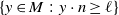$\{y\in M\,\colon y\cdot n\geq\ell\}$ and the set $\mathfrak{D}\cap\mathfrak{H}(\ell,n)$ .

But, by construction and convexity (see Figure 1),

\[u_{\mathfrak{D}_{\ell,n}}(y)=\begin{cases}u_{M}(y)& \text{if $ y\in M\cap\mathscr{H}^{\;\,+}$,}\\ -n & \text{if $ y\in \mathfrak{D}\cap\mathfrak{H}(\ell,n)$.}\end{cases}\]

Relation (4.33) would be obtained by plugging the above identity into (4.37). Now, using the fact that $\mathscr{H}^{\;\,+}$ and $\mathfrak{D}$ are open, one easily deduces that $\mathfrak{V}$ is contained on $\partial\mathfrak{D}_{\ell,n}$ . Finally, to see that (4.36) is satisfied, let us first recall that for any sets $E,F\subset\mathbb{R}^d$ it holds that (i) $d_{E}(q)=d_{\bar{E}}(q)$ , (ii) $d_{E}(q)=0$ if and only if $q\in\bar{E}$ , (iii) $d_{E\cap F}(q)\geq\max\{d_{E}(q),d_{F}(q)\}$ . Using these properties and the fact that $\mathfrak{D}_{\ell,n}$ is open, we conclude that the set $\mathcal{O}=(\bar{\mathscr{H}^{\;\,+}})^c\cup(\bar{\mathscr{H}^{\;\,+}}\cap\bar{\mathfrak{D}}^c)\cup\mathfrak{D}_{\ell,n}$ cannot belong to the boundary of $\mathfrak{D}_{\ell,n}$ . Furthermore,

\[\mathcal{O}^c=\mathfrak{V}\cup(M\cap\mathfrak{H}(\ell,n)) \quad\text{and}\quad \mathfrak{V}\cap(M\cap\mathfrak{H}(\ell,n))=\emptyset.\]

Hence

\[\partial\mathfrak{D}_{\ell,n}=\mathfrak{V}\cup(\partial\mathfrak{D}_{\ell,n}\cap(M\cap\mathfrak{H}(\ell,n))),\]

from which (4.36) readily follows.