


In memory of Phil Scott, 1947–2023
1. Introduction
A trace on a symmetric monoidal category $({\mathbf{C}},\oplus )$
is an operation that assigns to each map
$({\mathbf{C}},\oplus )$
is an operation that assigns to each map $f \colon {A\oplus X \rightarrow B\oplus X}$
another map
$f \colon {A\oplus X \rightarrow B\oplus X}$
another map ${\operatorname {Tr}}^{X} f \colon {A \rightarrow B}$
, satisfying some well-known axioms (Joyal et al., Reference Joyal, Street and Verity1996; Selinger, Reference Selinger and Coecke2011). In string diagrams, traces are represented by looping an output of
${\operatorname {Tr}}^{X} f \colon {A \rightarrow B}$
, satisfying some well-known axioms (Joyal et al., Reference Joyal, Street and Verity1996; Selinger, Reference Selinger and Coecke2011). In string diagrams, traces are represented by looping an output of $f$
back to the corresponding input, as in the following diagram.
$f$
back to the corresponding input, as in the following diagram.

In categories of vector spaces, there are two relevant monoidal structures: the “multiplicative” tensor $\otimes$
and the “additive” tensor
$\otimes$
and the “additive” tensor $\oplus$
, also known as biproduct or direct sum. The multiplicative tensor on finite-dimensional vector spaces has a well-known trace (induced by the compact closed structure). But in this paper, we are interested in the additive tensor.
$\oplus$
, also known as biproduct or direct sum. The multiplicative tensor on finite-dimensional vector spaces has a well-known trace (induced by the compact closed structure). But in this paper, we are interested in the additive tensor.
Linear maps between direct sums amount to block matrices: to specify a linear map $f \colon {A_1 \oplus \cdots \oplus A_n \rightarrow B_1 \oplus \cdots \oplus B_m}$
is to specify all of the components
$f \colon {A_1 \oplus \cdots \oplus A_n \rightarrow B_1 \oplus \cdots \oplus B_m}$
is to specify all of the components $f_{j i} \colon {A_i \rightarrow B_j}$
. We may organize this data either in a rectangular array as usual or in a string diagram (see Selinger (Reference Selinger and Coecke2011)), which will be illustrative.
$f_{j i} \colon {A_i \rightarrow B_j}$
. We may organize this data either in a rectangular array as usual or in a string diagram (see Selinger (Reference Selinger and Coecke2011)), which will be illustrative.

Composition, i.e., matrix multiplication, is given by summing over all paths from each input to each output.

Hence, a natural way to try to define an additive trace on a category of vector spaces is by the following sum-over-paths formula, motivated by the accompanying string diagram.

That is, we sum over all paths from the exposed input to the exposed output, as usual. However, the sum may not converge (supposing there is even any notion of convergence), and so the formula does not define a total operation. Indeed, there is no totally defined trace with respect to $\oplus$
on any category of finite (or infinite) dimensional vector spaces (Hoshino, Reference Hoshino2018).
$\oplus$
on any category of finite (or infinite) dimensional vector spaces (Hoshino, Reference Hoshino2018).
Therefore, it came as a surprise when Bartha (Reference Bartha2014) showed that the category of finite-dimensional Hilbert spaces and isometries has a well-defined additive trace. In particular, not only does Bartha’s trace of an isometry always exist, but it is again an isometry. By duality, Bartha’s trace also works for coisometries and therefore also for unitary maps. Moreover, Andrés-Martínez pointed out that Bartha’s trace further generalizes to all contractions (Andrés-Martínez, Reference Andrés-Martínez2022). These results suggest that there might be some physical interpretation of loops in quantum systems, but we do not know what it is.
In this paper, we show that Bartha’s result is not specifically tied to Hilbert spaces, but works in any dagger additive category with suitable additional structure. The specific additional structure that we need to assume is the existence of Moore–Penrose pseudoinverses.
In a nutshell, a pseudoinverse of an arrow $f \colon {A \rightarrow B}$
is an arrow
$f \colon {A \rightarrow B}$
is an arrow ${{f}^\circ } \colon {B \rightarrow A}$
such that both
${{f}^\circ } \colon {B \rightarrow A}$
such that both $f\circ {{f}^\circ }$
and
$f\circ {{f}^\circ }$
and ${{f}^\circ }\circ f$
are self-adjoint and
${{f}^\circ }\circ f$
are self-adjoint and ${{f}\circ f^\circ } \circ {f}=f$
and
${{f}\circ f^\circ } \circ {f}=f$
and ${{{f}^\circ }}\circ f\circ {{f}^\circ }={{f}^\circ }$
. Pseudoinverses are unique when they exist, and they generalize inverses. Moreover, the definition of pseudoinverse is purely algebraic and makes sense in any dagger category (Cockett and Lemay, Reference Cockett and Lemay2023).
${{{f}^\circ }}\circ f\circ {{f}^\circ }={{f}^\circ }$
. Pseudoinverses are unique when they exist, and they generalize inverses. Moreover, the definition of pseudoinverse is purely algebraic and makes sense in any dagger category (Cockett and Lemay, Reference Cockett and Lemay2023).
The reader may be wondering why pseudoinverses should appear in this context. Disregarding convergence issues, the sum-over-paths formula above is calculated by way of a geometric series:
 \begin{equation*}{\operatorname {Tr}}^{X}f = f_{B A}+{f_{B X}}\circ \left (\sum _{i = 0}^\infty {f_{X X}}^i \right )\circ f_{X A} = f_{B A} +{f_{B X}}\circ ({1}_{X} - f_{X X})^{-1}\circ f_{X A}.\end{equation*}
Bartha’s trace can be defined by simply changing the inverse in this formula, which may or may not exist, to a pseudoinverse. See Section 6 for more details.
Our main result is the following:
Theorem 1. Given any dagger additive category with pseudoinverses, there is a totally defined trace on each of the following monoidal subcategories:
-
• the unitaries,
-
• the isometries,
-
• the coisometries, and
-
• the contractions.
Moreover, in the cases of unitaries and contractions, which are dagger monoidal subcategories, the trace is a dagger trace.
After reviewing some background material in Section 2, we introduce contractions in Section 3 and pseudoinverses in Section 4 and prove some of their required properties. Section 5 is devoted to the proof of the main theorem.
The remaining sections contain additional observations that are not required for our main result, but are of independent interest. In Section 6, we discuss further properties of Bartha’s trace formula. In Section 7, we muse about the possibility of physical interpretations. Section 8 contains more results about pseudoinverses in dagger categories. Finally, in Section 9, we have collected various counterexamples.
2. Background
2.1 Dagger categories
We recall some basic definitions and properties of dagger categories to fix the notation for the rest of the paper. For a more detailed treatment, see Selinger (Reference Selinger2007), Heunen and Vicary (Reference Heunen and Vicary2019), Karvonen (Reference Karvonen2019).
Definition 2.1 (Dagger category). A dagger category is a category equipped with an identity-on-objects involutive contravariant functor, denoted $({\mathord {\text{-}}})^\dagger$
. In other words, for
$({\mathord {\text{-}}})^\dagger$
. In other words, for $f \colon {A \rightarrow B}$
, we have
$f \colon {A \rightarrow B}$
, we have $f^\dagger \colon {B \rightarrow A}$
, and we have the following properties:
$f^\dagger \colon {B \rightarrow A}$
, and we have the following properties:
-
• $f^{\dagger \dagger } = f$
,
$f^{\dagger \dagger } = f$
, -
•
$({1}_{A})^\dagger = {1}_{A}$
, and -
•
$(g\circ f)^\dagger = f^\dagger \circ g^\dagger$
.


For example, the category $\mathbf{Hilb}$
of Hilbert spaces and bounded linear maps is a dagger category. Its full subcategory
$\mathbf{Hilb}$
of Hilbert spaces and bounded linear maps is a dagger category. Its full subcategory $\mathbf{FdHilb}$
of finite-dimensional Hilbert spaces is also a dagger category.
$\mathbf{FdHilb}$
of finite-dimensional Hilbert spaces is also a dagger category.
Definition 2.2 (Properties of arrows). An arrow $f \colon {A \rightarrow B}$
in a dagger category is called an isometry if
$f \colon {A \rightarrow B}$
in a dagger category is called an isometry if $f^\dagger \circ f = {1}_{A}$
, a coisometry if
$f^\dagger \circ f = {1}_{A}$
, a coisometry if $f\circ f^\dagger = {1}_{B}$
, and unitary if it is an isometry and a coisometry. Equivalently,
$f\circ f^\dagger = {1}_{B}$
, and unitary if it is an isometry and a coisometry. Equivalently, $f$
is unitary if it is invertible and
$f$
is unitary if it is invertible and $f^{-1} = f^\dagger$
. An arrow
$f^{-1} = f^\dagger$
. An arrow $f \colon {A \rightarrow A}$
is self-adjoint (or hermitian) if
$f \colon {A \rightarrow A}$
is self-adjoint (or hermitian) if $f=f^\dagger$
.
$f=f^\dagger$
.
In this paper, we use the symbol $\oplus$
to denote the monoidal product, because we are mainly interested in monoidal structures that are induced by biproducts.
$\oplus$
to denote the monoidal product, because we are mainly interested in monoidal structures that are induced by biproducts.
Definition 2.3 (Dagger monoidal category). A dagger monoidal category is a dagger category that is also monoidal, such that $({\mathord {\text{-}}})^\dagger$
is a strict monoidal functor. More explicitly, this means that the monoidal structure isomorphisms (i.e., associators and unitors) are unitary, and for all arrows
$({\mathord {\text{-}}})^\dagger$
is a strict monoidal functor. More explicitly, this means that the monoidal structure isomorphisms (i.e., associators and unitors) are unitary, and for all arrows $f$
and
$f$
and $g$
, we have
$g$
, we have
 \begin{equation*} (f \oplus g)^\dagger = f^\dagger \oplus g^\dagger . \end{equation*}
In a dagger (monoidal) category, the isometries, the coisometries, and the unitary maps each form a (monoidal) subcategory, that is they are closed under compositions (and monoidal products).
Definition 2.4 (Dagger finite biproduct category). A dagger finite biproduct category is a dagger category that also has finite biproducts such that the projection maps $\pi _i \colon {A_1\oplus A_2 \rightarrow A_i}$
and the inclusion maps
$\pi _i \colon {A_1\oplus A_2 \rightarrow A_i}$
and the inclusion maps $\iota _i \colon {A_i \rightarrow A_1\oplus A_2}$
satisfy
$\iota _i \colon {A_i \rightarrow A_1\oplus A_2}$
satisfy $\pi _i = \iota _i^\dagger$
.
$\pi _i = \iota _i^\dagger$
.
As usual in any category with finite biproducts, there is a zero object $0$
, and we can define the addition of arrows
$0$
, and we can define the addition of arrows $f,g \colon {A \rightarrow B}$
in the usual way by
$f,g \colon {A \rightarrow B}$
in the usual way by $f+g = {A \rightarrow {A\oplus A \xrightarrow {f\oplus g} {B\oplus B \rightarrow B}}}$
. There are also zero maps
$f+g = {A \rightarrow {A\oplus A \xrightarrow {f\oplus g} {B\oplus B \rightarrow B}}}$
. There are also zero maps $0 \colon {A \rightarrow {0 \rightarrow B}}$
. Indeed, every finite biproduct category is enriched over commutative monoids. In the case of a dagger finite biproduct category, the dagger respects the commutative monoid structure. Not all categories enriched in commutative monoids have finite biproducts, and occasionally we will prefer not to assume the existence of biproducts in order to state results in the appropriate generality.
$0 \colon {A \rightarrow {0 \rightarrow B}}$
. Indeed, every finite biproduct category is enriched over commutative monoids. In the case of a dagger finite biproduct category, the dagger respects the commutative monoid structure. Not all categories enriched in commutative monoids have finite biproducts, and occasionally we will prefer not to assume the existence of biproducts in order to state results in the appropriate generality.
Definition 2.5 (Finite addition category). A finite addition category (or rigoid) is a category enriched in commutative monoids. Explicitly, a finite addition category is a category where every hom-set is equipped with the structure of a commutative monoid, subject to the distributive laws
 \begin{equation*}g\circ (f_1 + f_2) = g\circ f_1 + g\circ f_2, \quad (g_1 + g_2)\circ f = g_1\circ f + g_2\circ f, \quad \text{and} \quad 0\circ f = 0 = f\circ 0\end{equation*}
for all such arrows with appropriate domain and codomain.
A dagger finite addition category is a category that is both a dagger category and a finite addition category such that for all arrows $f \colon {A \rightarrow B}$
and
$f \colon {A \rightarrow B}$
and $g \colon {A \rightarrow B}$
we have
$g \colon {A \rightarrow B}$
we have
 \begin{equation*}(f + g)^\dagger = f^\dagger + g^\dagger .\end{equation*}
(Note $0^\dagger = 0$
by functoriality regardless.)
$0^\dagger = 0$
by functoriality regardless.)
Most important to us is the case where we also have subtraction.
Definition 2.6 (Negatives, additive category). We say that a finite addition category has negatives if for every $f \colon {A \rightarrow B}$
, there exists
$f \colon {A \rightarrow B}$
, there exists $-f \colon {A \rightarrow B}$
such that
$-f \colon {A \rightarrow B}$
such that $f + (-f) = 0$
. Note that this is the same as being enriched in abelian groups. A (dagger) finite biproduct category with negatives is called a (dagger) additive category.
$f + (-f) = 0$
. Note that this is the same as being enriched in abelian groups. A (dagger) finite biproduct category with negatives is called a (dagger) additive category.
We will also need the concept of positive map.
Definition 2.7 (Positive map). A map $a \colon {A \rightarrow A}$
in a dagger category is positive if there exists
$a \colon {A \rightarrow A}$
in a dagger category is positive if there exists $f \colon {A \rightarrow B}$
with
$f \colon {A \rightarrow B}$
with $a = f^\dagger \circ f$
.
$a = f^\dagger \circ f$
.
Positive maps in $\mathbf{Hilb}$
are positive operators in the usual sense. Every positive map is self-adjoint, and the sum of positive maps is positive if we have dagger biproducts. Given two maps
$\mathbf{Hilb}$
are positive operators in the usual sense. Every positive map is self-adjoint, and the sum of positive maps is positive if we have dagger biproducts. Given two maps $f,g \colon {A \rightarrow A}$
in a dagger finite biproduct category, we say that
$f,g \colon {A \rightarrow A}$
in a dagger finite biproduct category, we say that $f\leq g$
if there exists some positive
$f\leq g$
if there exists some positive $a$
such that
$a$
such that $g=f+a$
. The dagger biproducts ensure that
$g=f+a$
. The dagger biproducts ensure that $\leq$
is a partial order.
$\leq$
is a partial order.
Lemma 2.8.
Let $f,g \colon {A \rightarrow A}$
be arrows in a dagger finite biproduct category and assume
$f,g \colon {A \rightarrow A}$
be arrows in a dagger finite biproduct category and assume $f\leq g$
.
$f\leq g$
.
-
(a) For all
$h \colon {A \rightarrow B}$
, we have
$ h\circ f \circ {h}^\dagger \leq h \circ g\circ {h}^\dagger$
. -
(b) For all
$f',g' \colon {A' \rightarrow A'}$
with
$f'\leq g'$
, we have
$f\oplus f'\leq g\oplus g'$
.


Proof.
Since $g=f+a$
and
$g=f+a$
and $g' = f'+a'$
for some positive
$g' = f'+a'$
for some positive $a$
and
$a$
and $a'$
, we have
$a'$
, we have
 \begin{equation*}h\circ g\circ {h}^\dagger =h\circ f\circ {h}^\dagger +h\circ a\circ {h}^\dagger \quad \text{and} \quad g \oplus g' = (f + a) \oplus (f'+ a') = (f \oplus f') + (a \oplus a').\end{equation*}
It is easy to see $h \circ a\circ {h}^\dagger$
and
$h \circ a\circ {h}^\dagger$
and $a \oplus a'$
are positive, which implies both claims.
$a \oplus a'$
are positive, which implies both claims.
2.2 Matrices
It is well-known that maps $f \colon {A_1 \oplus \cdots \oplus A_m \rightarrow B_1 \oplus \cdots \oplus B_n}$
in a finite biproduct category are in one-to-one correspondence with matrices
$f \colon {A_1 \oplus \cdots \oplus A_m \rightarrow B_1 \oplus \cdots \oplus B_n}$
in a finite biproduct category are in one-to-one correspondence with matrices $(f_{j i})$
, where
$(f_{j i})$
, where $f_{j i} \colon {A_i \rightarrow B_j}$
. Here we describe this correspondence in more detail.
$f_{j i} \colon {A_i \rightarrow B_j}$
. Here we describe this correspondence in more detail.
Let $\mathbf{C}$
be a finite addition category, and let
$\mathbf{C}$
be a finite addition category, and let
 \begin{equation*}\mathbf{A} = \{A_i\}_{i \in I} \qquad \text{and} \qquad \mathbf{B} = \{B_j\}_{j \in J}\end{equation*}
be finite families of objects in $\mathbf{C}$
.
$\mathbf{C}$
.
Definition 2.9 (Matrices). A matrix $f \colon {\mathbf{A} \rightarrow \mathbf{B}}$
consists of an arrow
$f \colon {\mathbf{A} \rightarrow \mathbf{B}}$
consists of an arrow $f_{_{j i}} \colon {A_i \rightarrow B_j}$
in
$f_{_{j i}} \colon {A_i \rightarrow B_j}$
in $\mathbf{C}$
for each
$\mathbf{C}$
for each $i \in I$
and
$i \in I$
and $j \in J$
.
$j \in J$
.
If $f \colon {\{A_i\}_{i \in I} \rightarrow \{B_j\}_{j \in J}}$
and
$f \colon {\{A_i\}_{i \in I} \rightarrow \{B_j\}_{j \in J}}$
and $g \colon {\{B_j\}_{j \in J} \rightarrow \{C_k\}_{k \in K}}$
are matrices, their composition (or product)
$g \colon {\{B_j\}_{j \in J} \rightarrow \{C_k\}_{k \in K}}$
are matrices, their composition (or product) $g\circ f \colon {\{A_i\}_{i \in I} \rightarrow \{C_k\}_{k \in K}}$
is given by the usual matrix multiplication formula
$g\circ f \colon {\{A_i\}_{i \in I} \rightarrow \{C_k\}_{k \in K}}$
is given by the usual matrix multiplication formula
 \begin{equation*}(g\circ f)_{_{k i}} = \sum _{j \in J}g_{_{k j}}\circ f_{_{j i}}\end{equation*}
(where the summation notation refers to addition via $+$
).
$+$
).
We denote the category of finite families of objects in $\mathbf{C}$
and matrices by
$\mathbf{C}$
and matrices by $\mathbf{Mat}({\mathbf{C}})$
. Note that
$\mathbf{Mat}({\mathbf{C}})$
. Note that $\mathbf{Mat}({\mathbf{C}})$
is a finite biproduct category. Moreover, if
$\mathbf{Mat}({\mathbf{C}})$
is a finite biproduct category. Moreover, if $\mathbf{C}$
is a dagger finite addition category, then
$\mathbf{C}$
is a dagger finite addition category, then $\mathbf{Mat}({\mathbf{C}})$
is a dagger finite biproduct category, where for each matrix
$\mathbf{Mat}({\mathbf{C}})$
is a dagger finite biproduct category, where for each matrix $f \colon {\{A_i\}_{i \in I} \rightarrow \{B_j\}_{j \in J}}$
we take
$f \colon {\{A_i\}_{i \in I} \rightarrow \{B_j\}_{j \in J}}$
we take $(f^\dagger )_{_{j i}} = (f_{_{i j}})^\dagger$
for all
$(f^\dagger )_{_{j i}} = (f_{_{i j}})^\dagger$
for all $i\in I$
,
$i\in I$
, $j \in J$
.
$j \in J$
.
When $\mathbf{C}$
is already a (dagger) finite biproduct category,
$\mathbf{C}$
is already a (dagger) finite biproduct category, $\mathbf{Mat}({\mathbf{C}})$
is (dagger) equivalent to
$\mathbf{Mat}({\mathbf{C}})$
is (dagger) equivalent to $\mathbf{C}$
. Indeed,
$\mathbf{C}$
. Indeed, $\mathbf{C}$
fully and faithfully embeds in
$\mathbf{C}$
fully and faithfully embeds in $\mathbf{Mat}({\mathbf{C}})$
as matrices between single objects, and moreover, this embedding is essentially surjective: given an arbitrary finite family
$\mathbf{Mat}({\mathbf{C}})$
as matrices between single objects, and moreover, this embedding is essentially surjective: given an arbitrary finite family $\{A_i\}_{i \in I}$
with biproduct
$\{A_i\}_{i \in I}$
with biproduct $A$
in
$A$
in $\mathbf{C}$
, the canonical matrix
$\mathbf{C}$
, the canonical matrix $\{A\} \rightarrow \{A_i\}_{i \in I}$
whose entries are product projection maps is (unitarily) invertible.
$\{A\} \rightarrow \{A_i\}_{i \in I}$
whose entries are product projection maps is (unitarily) invertible.
Hence, arrows $A_1 \oplus \cdots \oplus A_m \rightarrow B_1 \oplus \cdots \oplus B_n$
are in canonical correspondence with matrices
$A_1 \oplus \cdots \oplus A_m \rightarrow B_1 \oplus \cdots \oplus B_n$
are in canonical correspondence with matrices $\{A_i\}_{i=1}^m \rightarrow \{B_j\}_{j=1}^n$
. For
$\{A_i\}_{i=1}^m \rightarrow \{B_j\}_{j=1}^n$
. For $f \colon {A_1 \oplus \cdots \oplus A_m \rightarrow B_1 \oplus \cdots \oplus B_n}$
, we write
$f \colon {A_1 \oplus \cdots \oplus A_m \rightarrow B_1 \oplus \cdots \oplus B_n}$
, we write
 \begin{equation*} \renewcommand{\arraystretch}{1.1} f\; = \;\;\; \begin{array}[b]{cc} & \begin{array}{ccccc} {\scriptstyle A_1} & {\scriptstyle \oplus } & {\scriptstyle \cdots } & {\scriptstyle \oplus } & {\scriptstyle A_m} \end{array} \\ \begin{array}{c} {\scriptstyle B_1}\\[-2.5pt] {\scriptstyle \oplus}\\[-2.5pt] {{\scriptstyle \vdots }}\\[-2.5pt] {\scriptstyle \oplus }\\[-2.5pt] {\scriptstyle B_n}\\[4pt] \end{array}& \begin{pmatrix} f_{1 1} && \cdots && f_{1 m} \\[-4pt] && && \\[-4pt] \vdots && \ddots && \vdots \\[-4pt] && && \\[-4pt] f_{n 1} && \cdots && f_{n m} \\[4pt] \end{pmatrix} \end{array}. \end{equation*}
where $f_{_{j i}}$
is the canonical arrow
$f_{_{j i}}$
is the canonical arrow
 \begin{equation*}{A_i \rightarrow {(A_1 \oplus \cdots \oplus A_m) \xrightarrow {f} {(B_1 \oplus \cdots \oplus B_n) \rightarrow B_j}}}.\end{equation*}
We also frequently abuse notation and write $f_{_{B_j A_i}}$
to mean
$f_{_{B_j A_i}}$
to mean $f_{_{j i}}$
. Given a matrix
$f_{_{j i}}$
. Given a matrix
 \begin{equation*} f = \begin{pmatrix}f_{1 1}\;\; &f_{1 2}\\f_{2 1}\;\; &f_{2 2}\end{pmatrix} \colon {A_1\oplus A_2 \rightarrow B_1\oplus B_2}, \end{equation*}
we call each $f_{j i} \colon {A_i \rightarrow B_j}$
a component of
$f_{j i} \colon {A_i \rightarrow B_j}$
a component of $f$
, we call
$f$
, we call $\left (\begin{smallmatrix}f_{1 i}\\f_{2 i}\end{smallmatrix}\right ) \colon {A_i \rightarrow B_1\oplus B_2}$
a column of
$\left (\begin{smallmatrix}f_{1 i}\\f_{2 i}\end{smallmatrix}\right ) \colon {A_i \rightarrow B_1\oplus B_2}$
a column of $f$
, and we call
$f$
, and we call $\left (\begin{smallmatrix}f_{j 1}\,f_{j 2}\end{smallmatrix}\right ) \colon {A_1\oplus A_2 \rightarrow B_j}$
a row of
$\left (\begin{smallmatrix}f_{j 1}\,f_{j 2}\end{smallmatrix}\right ) \colon {A_1\oplus A_2 \rightarrow B_j}$
a row of $f$
. We use analogous terminology for larger matrices.
$f$
. We use analogous terminology for larger matrices.
Remark 2.10. In a dagger finite biproduct category, an arrow of the form
 \begin{equation*} \begin{array}{cc}& \begin{array}{ccccc} {\scriptstyle A_1} & {\scriptstyle \oplus } & {\scriptstyle \cdots } & {\scriptstyle \oplus } & {\scriptstyle A_m} \end{array}\\[-2pt] {\scriptstyle B}\;\;&\begin{pmatrix} f_1 &\;\;& \cdots &\;\;& f_m \\ \end{pmatrix} \end{array} \end{equation*}
is an isometry if and only if $f_i^\dagger \circ f_i = {1}_{A_i}$
for all
$f_i^\dagger \circ f_i = {1}_{A_i}$
for all $i$
and
$i$
and $f_j^\dagger \circ f_i = 0$
for
$f_j^\dagger \circ f_i = 0$
for $i\neq j$
.
$i\neq j$
.
Remark 2.11. In a dagger additive category, every isometry is a component of a unitary. Indeed, suppose $f \colon {A \rightarrow B}$
is an isometry. Then the following arrow is unitary.
$f \colon {A \rightarrow B}$
is an isometry. Then the following arrow is unitary.
 \begin{equation*} \begin{array}{cc}&\begin{array}{ccccccccc} {\scriptstyle A} & \;\quad{\scriptstyle \oplus}\; & \quad{\scriptstyle B}\quad\;\;\; \\\end{array}\\ \begin{array}{cc}{\scriptstyle A} \\[-0.5ex]{\scriptstyle \oplus} \\[-0.5ex]{\scriptstyle B} \\\end{array} & \begin{pmatrix} \,\,0 && \quad f^\dagger \\[-0.5ex] &&\\[-0.5ex] \,\,f && \quad {1}_{B} - f\circ f^\dagger \\ \end{pmatrix}\end{array} \end{equation*}
2.3 Dagger idempotents
Definition 2.12 (Dagger idempotents). A arrow $p \colon {A \rightarrow A}$
is called a dagger idempotent (or projection) if
$p \colon {A \rightarrow A}$
is called a dagger idempotent (or projection) if $p = p\circ p=p^{\dagger }$
.
$p = p\circ p=p^{\dagger }$
.
Whenever $f \colon {B \rightarrow A}$
is an isometry, then
$f \colon {B \rightarrow A}$
is an isometry, then $p = f\circ f^\dagger$
is a dagger idempotent. If
$p = f\circ f^\dagger$
is a dagger idempotent. If $p$
is of this form, we say that
$p$
is of this form, we say that $p$
is dagger split. When dagger splittings exist, they are unique up to unitary isomorphism. Moreover, unlike ordinary idempotents, dagger idempotents are uniquely determined by their image (see Selinger (Reference Selinger2008)).
$p$
is dagger split. When dagger splittings exist, they are unique up to unitary isomorphism. Moreover, unlike ordinary idempotents, dagger idempotents are uniquely determined by their image (see Selinger (Reference Selinger2008)).
The idempotent completion of a category is a staple of ordinary category theory; the dagger idempotent completion, from Selinger (Reference Selinger2008), is the analogue for dagger categories.
Definition 2.13 (Dagger idempotent completion). A morphism of idempotents from an idempotent $p \colon {A \rightarrow A}$
to an idempotent
$p \colon {A \rightarrow A}$
to an idempotent $q \colon {B \rightarrow B}$
in a category
$q \colon {B \rightarrow B}$
in a category $\mathbf{C}$
is an arrow
$\mathbf{C}$
is an arrow $f \colon {A \rightarrow B}$
in
$f \colon {A \rightarrow B}$
in $\mathbf{C}$
such that
$\mathbf{C}$
such that $f = {q} \circ f\circ p$
(equivalently,
$f = {q} \circ f\circ p$
(equivalently, $f\circ p = f = q\circ f$
).
$f\circ p = f = q\circ f$
).
The category consisting of idempotents in $\mathbf{C}$
and morphisms of idempotents between them is called the idempotent completion (or Karoubi envelope or Cauchy completion) of
$\mathbf{C}$
and morphisms of idempotents between them is called the idempotent completion (or Karoubi envelope or Cauchy completion) of $\mathbf{C}$
, denoted
$\mathbf{C}$
, denoted $\mathbf{Split}({\mathbf{C}})$
. Note this is indeed a category, with
$\mathbf{Split}({\mathbf{C}})$
. Note this is indeed a category, with $p \colon {p \rightarrow p}$
acting as
$p \colon {p \rightarrow p}$
acting as $1_{p}$
.
$1_{p}$
.
When $\mathbf{C}$
is moreover a dagger category, the full subcategory of
$\mathbf{C}$
is moreover a dagger category, the full subcategory of $\mathbf{Split}({\mathbf{C}})$
spanned by dagger idempotents is called the dagger idempotent completion (or the dagger Karoubi envelope) of
$\mathbf{Split}({\mathbf{C}})$
spanned by dagger idempotents is called the dagger idempotent completion (or the dagger Karoubi envelope) of $\mathbf{C}$
, denoted
$\mathbf{C}$
, denoted $\mathbf{Split}_{\dagger }({\mathbf{C}})$
. Note this is indeed a dagger category, with the dagger taken as in
$\mathbf{Split}_{\dagger }({\mathbf{C}})$
. Note this is indeed a dagger category, with the dagger taken as in $\mathbf{C}$
.
$\mathbf{C}$
.
Moreover, all structure of interest (e.g., monoidal structure, biproducts, addition, negatives, and, as we will later introduce, pseudoinverses (Cockett and Lemay, Reference Cockett and Lemay2023)) on a dagger category transports to its dagger idempotent completion.
Next, we discuss the relationship between idempotents and additive structure.
Definition 2.14 (Complementary idempotents). Two idempotents $p,q \colon {A \rightarrow A}$
in a finite addition category are complementary if
$p,q \colon {A \rightarrow A}$
in a finite addition category are complementary if $p + q = {1}_{A}$
and
$p + q = {1}_{A}$
and $q\circ p = 0 = p\circ q$
.
$q\circ p = 0 = p\circ q$
.
If the category has negatives, complements always exist, because whenever $p$
is an idempotent, so is
$p$
is an idempotent, so is $1-p$
. It is obvious that the complement is unique in that case. Interestingly, uniqueness even holds without assuming negatives.
$1-p$
. It is obvious that the complement is unique in that case. Interestingly, uniqueness even holds without assuming negatives.
Lemma 2.15 (Uniqueness of complementary idempotent). Let $p \colon {A \rightarrow A}$
be an idempotent in a finite addition category. If each of
$p \colon {A \rightarrow A}$
be an idempotent in a finite addition category. If each of $q_1,q_2 \colon {A \rightarrow A}$
is a complementary idempotent of
$q_1,q_2 \colon {A \rightarrow A}$
is a complementary idempotent of $p$
, then
$p$
, then $q_1 = q_2$
.
$q_1 = q_2$
.
Proof. We have
 \begin{equation*}q_1 = (p + q_2)\circ q_1 = q_2\circ q_1 = q_2\circ (p + q_1) = q_2. \end{equation*}
Lemma 2.16 (Complementary dagger idempotents). Let $p, q \colon {A \rightarrow A}$
be complementary idempotents in a dagger finite addition category. Then
$p, q \colon {A \rightarrow A}$
be complementary idempotents in a dagger finite addition category. Then $p$
is a dagger idempotent if and only if
$p$
is a dagger idempotent if and only if $q$
is.
$q$
is.
Proof.
Suppose $p$
is a dagger idempotent. Then
$p$
is a dagger idempotent. Then
 \begin{equation*}p + q^\dagger = (p + q)^\dagger = 1_A\end{equation*}
and
 \begin{equation*}q^\dagger \circ p = (p\circ q)^\dagger = 0 = (q\circ p)^\dagger = p^\dagger \circ q.\end{equation*}
That is, $p$
and
$p$
and $q^\dagger$
are complementary. Hence
$q^\dagger$
are complementary. Hence $q = q^\dagger$
by Lemma 2.15.
$q = q^\dagger$
by Lemma 2.15.
Complementary dagger idempotents are an algebraic abstraction of orthogonal complement subspace projections.
Lemma 2.17 (Direct sum decomposition). Consider a (dagger) finite addition category in which all (dagger) idempotents (dagger) split. Given an object $A$
with complementary idempotents
$A$
with complementary idempotents $p,q \colon {A \rightarrow A}$
, there exist objects
$p,q \colon {A \rightarrow A}$
, there exist objects $A_1,A_2$
with
$A_1,A_2$
with $A = A_1 \oplus A_2$
such that
$A = A_1 \oplus A_2$
such that
 \begin{equation*} p = \; \begin{array}[b]{cc} & \begin{matrix} {\scriptstyle A_1} & {\scriptstyle \oplus } & {\scriptstyle A_2} \end{matrix}\\ \begin{matrix} {\scriptstyle A_1}\\[-1ex] {\scriptstyle \oplus }\\[-1ex] {\scriptstyle A_2} \end{matrix} & \begin{pmatrix} 1 & &\quad 0 \\[-1ex] & & \\[-1ex] 0 & &\quad 0 \end{pmatrix} \end{array} \quad and \quad q = \; \begin{array}[b]{cc} & \begin{matrix} {\scriptstyle A_1} & {\scriptstyle \oplus } & {\scriptstyle A_2} \end{matrix}\\ \begin{matrix} {\scriptstyle A_1}\\[-1ex] {\scriptstyle \oplus }\\[-1ex] {\scriptstyle A_2} \end{matrix} & \begin{pmatrix} 0 & &\quad 0 \\[-1ex] & & \\[-1ex] 0 & &\quad 1 \end{pmatrix} \end{array} \end{equation*}
Moreover, the factorization is unique up to (unitary) isomorphisms of the direct sum factors.
Axioms for a partially traced category. Here, we write ![]() for directed Kleene equality, i.e., if
for directed Kleene equality, i.e., if $x$
is defined, then so is
$x$
is defined, then so is $y$
and they are equal. Similarly,
$y$
and they are equal. Similarly, $x\rightleftharpoons y$
means
$x\rightleftharpoons y$
means $x$
and
$x$
and $y$
are either both undefined, or both defined and equal. The axioms for a total trace are obtained by replacing the symbols
$y$
are either both undefined, or both defined and equal. The axioms for a total trace are obtained by replacing the symbols ![]() and
and $\rightleftharpoons$
by equality.
$\rightleftharpoons$
by equality.

Proof idea.
Let $A_1$
be a splitting of
$A_1$
be a splitting of $p$
, and let
$p$
, and let $A_2$
be a splitting of
$A_2$
be a splitting of $q$
. The claimed properties are easy to verify.
$q$
. The claimed properties are easy to verify.
Remark 2.18. In Lemma 2.17 and elsewhere, we write $A=A_1\oplus A_2$
instead of
$A=A_1\oplus A_2$
instead of $A\cong A_1\oplus A_2$
; this is justified because (dagger) biproducts are defined up to (unitary) isomorphism in the first place.
$A\cong A_1\oplus A_2$
; this is justified because (dagger) biproducts are defined up to (unitary) isomorphism in the first place.
2.4 Trace
Recall that a trace on a symmetric monoidal category $\mathbf{C}$
is a family of operations
$\mathbf{C}$
is a family of operations ${\operatorname {Tr}}^{X} \colon {{\mathbf{C}}(A\oplus X,B\oplus X) \rightarrow {\mathbf{C}}(A,B)}$
, subject to a small number of axioms (Joyal et al., Reference Joyal, Street and Verity1996; Selinger, Reference Selinger and Coecke2011; Malherbe et al., Reference Malherbe, Scott and Selinger2012). The concept of a partial trace is defined similarly, except that
${\operatorname {Tr}}^{X} \colon {{\mathbf{C}}(A\oplus X,B\oplus X) \rightarrow {\mathbf{C}}(A,B)}$
, subject to a small number of axioms (Joyal et al., Reference Joyal, Street and Verity1996; Selinger, Reference Selinger and Coecke2011; Malherbe et al., Reference Malherbe, Scott and Selinger2012). The concept of a partial trace is defined similarly, except that ${\operatorname {Tr}}^{X}$
is a partially defined operation (Haghverdi and Scott, Reference Haghverdi and Scott2010). The axioms are shown in Figure 1. Note that a total trace is just a partial trace that happens to be totally defined. It was shown by Malherbe (Reference Malherbe2010) and Malherbe et al. (Reference Malherbe, Scott and Selinger2012) that every partially traced category can be faithfully embedded in a totally traced one, and conversely, every monoidal subcategory of a totally traced category is partially traced.
${\operatorname {Tr}}^{X}$
is a partially defined operation (Haghverdi and Scott, Reference Haghverdi and Scott2010). The axioms are shown in Figure 1. Note that a total trace is just a partial trace that happens to be totally defined. It was shown by Malherbe (Reference Malherbe2010) and Malherbe et al. (Reference Malherbe, Scott and Selinger2012) that every partially traced category can be faithfully embedded in a totally traced one, and conversely, every monoidal subcategory of a totally traced category is partially traced.
Remarkably, the sum-over-paths formula described in the introduction, ${\operatorname {Tr}}^{X}f = f_{B A} + {f_{B X}} \circ ({1}_{X} - f_{X X})^{-1}\circ f_{X A}$
, gives a partial trace on any additive category (Haghverdi and Scott, Reference Haghverdi and Scott2010; Hoshino, Reference Hoshino2018). More relevant to us is the following partial trace from Malherbe et al. (Reference Malherbe, Scott and Selinger2012), which agrees with the sum-over-paths formula when
${\operatorname {Tr}}^{X}f = f_{B A} + {f_{B X}} \circ ({1}_{X} - f_{X X})^{-1}\circ f_{X A}$
, gives a partial trace on any additive category (Haghverdi and Scott, Reference Haghverdi and Scott2010; Hoshino, Reference Hoshino2018). More relevant to us is the following partial trace from Malherbe et al. (Reference Malherbe, Scott and Selinger2012), which agrees with the sum-over-paths formula when $({1}_{X} - f_{X X})^{-1}$
exists, but which is also defined for more arrows.
$({1}_{X} - f_{X X})^{-1}$
exists, but which is also defined for more arrows.
Definition 2.19 (Kernel-image trace). Let $f \colon {A \oplus X \rightarrow B \oplus X}$
be an arrow in an additive category. The kernel-image trace
$f \colon {A \oplus X \rightarrow B \oplus X}$
be an arrow in an additive category. The kernel-image trace ${{\operatorname {Tr}}^{X}_{\text{ki}}}\ f \colon {A \rightarrow B}$
is defined if there exist arrows
${{\operatorname {Tr}}^{X}_{\text{ki}}}\ f \colon {A \rightarrow B}$
is defined if there exist arrows $i \colon {A \rightarrow X}$
and
$i \colon {A \rightarrow X}$
and $k \colon {X \rightarrow B}$
such that
$k \colon {X \rightarrow B}$
such that
 \begin{equation*} f_{X A} = ({1}_{X} - f_{X X})\circ i \qquad \text{and}\qquad k\circ ({1}_{X} - f_{X X}) = f_{B X}, \end{equation*}
as in the following commutative diagram

In this case, we define
 \begin{equation*}{{\operatorname {Tr}}^{X}_{\text{ki}}}\ f = f_{B A} +{k}\circ ({1}_{X} - f_{X X})\circ i.\end{equation*}
(Otherwise, the kernel-image trace is undefined.) Note ${\operatorname {Tr}}^{X}_{\text{ki}}$
is independent of the choice of each
${\operatorname {Tr}}^{X}_{\text{ki}}$
is independent of the choice of each $i$
and
$i$
and $k$
, since
$k$
, since
 \begin{equation*}f_{B A} + f_{B X}\circ i = {{\operatorname {Tr}}^{X}_{\text{ki}}}\ f = f_{B A} + k\circ f_{X A}.\end{equation*}
Proposition 2.20 (Malherbe et al., Reference Malherbe, Scott and Selinger2012). The kernel-image trace is a partial trace.
Remark 2.21. In a dagger category, a (partial) trace is called a dagger (partial) trace if ${\operatorname {Tr}}(f^{\dagger })=({\operatorname {Tr}} f)^\dagger$
. In a dagger additive category, the kernel-image trace is always a dagger partial trace, because its definition is self-dual.
${\operatorname {Tr}}(f^{\dagger })=({\operatorname {Tr}} f)^\dagger$
. In a dagger additive category, the kernel-image trace is always a dagger partial trace, because its definition is self-dual.
The kernel-image trace (Definition2.19) is quite central in this paper: we will prove Theorem1 by showing that the kernel-image trace is totally defined and hence gives a total trace on the desired subcategories.
3. Contractions
3.1 Basic properties
In the category of Hilbert spaces, a contraction is a map $f \colon {A \rightarrow B}$
such that for all
$f \colon {A \rightarrow B}$
such that for all $v\in A$
,
$v\in A$
, $\|f(v)\|\leq \|v\|$
. The following definition generalizes this concept to arbitrary dagger additive categories.
$\|f(v)\|\leq \|v\|$
. The following definition generalizes this concept to arbitrary dagger additive categories.
Definition 3.1 (Contraction). A contraction in a dagger additive category is an arrow $f \colon {A \rightarrow B}$
such that
$f \colon {A \rightarrow B}$
such that $f^\dagger \circ f \leq {1}_{A}$
. In other words, such that there exists an arrow
$f^\dagger \circ f \leq {1}_{A}$
. In other words, such that there exists an arrow $g \colon {A \rightarrow B'}$
with
$g \colon {A \rightarrow B'}$
with $f^\dagger \circ f + g^\dagger \circ g = {1}_{A}$
. Note that this is the case if and only if the map
$f^\dagger \circ f + g^\dagger \circ g = {1}_{A}$
. Note that this is the case if and only if the map $\left (\begin{smallmatrix}f\\g\end{smallmatrix}\right ) \colon {A \rightarrow B\oplus B'}$
is an isometry. A cocontraction is defined dually.
$\left (\begin{smallmatrix}f\\g\end{smallmatrix}\right ) \colon {A \rightarrow B\oplus B'}$
is an isometry. A cocontraction is defined dually.
In particular, every isometry, coisometry, and unitary map is a contraction. Also, biproduct projections and injections are contractions.
Note that Definition3.1 could be stated in a dagger finite addition category even without assuming negatives or biproducts, but many of the useful properties of contractions rely on the full dagger additive structure. A point in case is the next proposition, which gives several alternative characterizations of contractions, none of which would be equivalent in the absence of negatives (see Counterexamples 9.18 and 9.19).
Proposition 3.2 (Characterizations of contractions). Let $f \colon {A \rightarrow B}$
be an arrow in a dagger additive category. The following are equivalent.
$f \colon {A \rightarrow B}$
be an arrow in a dagger additive category. The following are equivalent.
-
(a)
$f$
is a component of a unitary.
-
(b)
$f$
is a contraction.
-
(c)
$f$
is a cocontraction.
-
(d)
$f$
is of the form
$e\circ m$
for some isometry
$m \colon {A \rightarrow X}$
and coisometry
$e \colon {X \rightarrow B}$
. -
(e)
$f$
is a composition of isometries and coisometries.


We delay the proof until we have established some lemmas. The following lemma tells us that contractions, like isometries, form a monoidal subcategory.
Lemma 3.3. Contractions are closed under composition and monoidal products.
Proof.
For composition, let $f \colon {A \rightarrow B}$
and
$f \colon {A \rightarrow B}$
and $g \colon {B \rightarrow C}$
be contractions. Then,
$g \colon {B \rightarrow C}$
be contractions. Then, $f^\dagger \circ f\leq {1}_{A}$
and
$f^\dagger \circ f\leq {1}_{A}$
and $g^\dagger \circ g\leq {1}_{B}$
. Using Lemma2.8 (a), we get
$g^\dagger \circ g\leq {1}_{B}$
. Using Lemma2.8 (a), we get
 \begin{equation*} (g\circ f)^\dagger \circ (g\circ f) ={f^\dagger }\circ {g^\dagger }\circ g\circ f \leq {f^\dagger } \circ {1}_{B}\circ f = f^\dagger \circ f \leq {1}_{A}. \end{equation*}
Therefore, $f\circ g$
is a contraction. For monoidal products, let
$f\circ g$
is a contraction. For monoidal products, let $f \colon {A \rightarrow B}$
and
$f \colon {A \rightarrow B}$
and $g \colon {A' \rightarrow B'}$
be contractions. Using Lemma2.8 (b), we get
$g \colon {A' \rightarrow B'}$
be contractions. Using Lemma2.8 (b), we get
 \begin{equation*} (f\oplus g)^\dagger \circ (f\oplus g) = (f^\dagger \circ f)\oplus (g^\dagger \circ g) \leq {1}_{A}\oplus {1}_{A'} = {1}_{A \oplus A'}. \end{equation*}
Therefore, $f\oplus g$
is a contraction.
$f\oplus g$
is a contraction.
Lemma 3.4 (Contractions as components of unitaries). In a dagger additive category, contractions are precisely the components of unitaries. In particular, contractions coincide with cocontractions.
Proof.
First, a component of a unitary is a composition of three contractions $u_{jk} ={\pi _j}\circ u\circ \iota _k$
and is therefore a contraction itself. Conversely, every contraction is a component of an isometry (as remarked in Definition3.1), which in turn is a component of a unitary by Remark2.11. Finally, since being a component of a unitary is a self-dual concept, so is being a contraction.
$u_{jk} ={\pi _j}\circ u\circ \iota _k$
and is therefore a contraction itself. Conversely, every contraction is a component of an isometry (as remarked in Definition3.1), which in turn is a component of a unitary by Remark2.11. Finally, since being a component of a unitary is a self-dual concept, so is being a contraction.
We can now prove Proposition3.2.
Proof of Proposition
3.2. The equivalence (a) $\iff$
(b)
$\iff$
(b) $\iff$
(c) is Lemma3.4. For (b)
$\iff$
(c) is Lemma3.4. For (b) $\implies$
(d), assume
$\implies$
(d), assume $f^\dagger \circ f+g^\dagger \circ g={1}$
. Then
$f^\dagger \circ f+g^\dagger \circ g={1}$
. Then $f=e\circ m$
, where
$f=e\circ m$
, where $e=({1}\,\,0\,)$
is a coisometry and
$e=({1}\,\,0\,)$
is a coisometry and $m=\left (\begin{smallmatrix}f\\g\end{smallmatrix}\right )$
is an isometry. The implication (d)
$m=\left (\begin{smallmatrix}f\\g\end{smallmatrix}\right )$
is an isometry. The implication (d) $\implies$
(e) is trivial, and (e)
$\implies$
(e) is trivial, and (e) $\implies$
(b) follows because contractions are closed under composition by Lemma3.3.
$\implies$
(b) follows because contractions are closed under composition by Lemma3.3.
3.2 Contractions and definiteness
Contractions have even better properties when the underlying dagger category satisfies the following condition.
Definition 3.5 (Definite). A dagger category with a zero object is definite if for all arrows $f$
, we have that
$f$
, we have that $f^\dagger \circ f = 0$
implies
$f^\dagger \circ f = 0$
implies $f = 0$
.
$f = 0$
.
In the familiar context of Hilbert spaces, the columns or rows of a contraction have norm at most $1$
. An analogue of this principle holds in any definite dagger additive category.
$1$
. An analogue of this principle holds in any definite dagger additive category.
Lemma 3.6 (Maxed-out column). In a definite dagger additive category, assume $f=\left (\begin{smallmatrix}f_1\\f_2\end{smallmatrix}\right )$
is a contraction. If
$f=\left (\begin{smallmatrix}f_1\\f_2\end{smallmatrix}\right )$
is a contraction. If $f_1$
is an isometry, then
$f_1$
is an isometry, then $f_2=0$
.
$f_2=0$
.
Proof.
It suffices to show the result when $f$
is an isometry, because every contraction is a row of an isometry. We have
$f$
is an isometry, because every contraction is a row of an isometry. We have ${1}_{A} = f^\dagger \circ f = f_1^\dagger \circ f_1 + f_2^\dagger \circ f_2 = {1}_{A} + f_2^\dagger \circ f_2$
. Subtracting
${1}_{A} = f^\dagger \circ f = f_1^\dagger \circ f_1 + f_2^\dagger \circ f_2 = {1}_{A} + f_2^\dagger \circ f_2$
. Subtracting ${1}_{A}$
from both sides, we get
${1}_{A}$
from both sides, we get $0 = f_2^\dagger \circ f_2$
. Now by definiteness,
$0 = f_2^\dagger \circ f_2$
. Now by definiteness, $f_2 = 0$
.
$f_2 = 0$
.
Corollary 3.7 (Maxed-out row and column). In a definite dagger additive category, assume
 \begin{equation*} f = \begin{pmatrix}{1}\;\;\;\; & f_{12} \\ f_{21}\;\;\;\; & f_{22}\\[4pt] \end{pmatrix} \end{equation*}
is a contraction. Then, $f_{12}=0$
and
$f_{12}=0$
and $f_{21}=0$
.
$f_{21}=0$
.
Proof. $f_{12}=0$
follows from Lemma3.6 and
$f_{12}=0$
follows from Lemma3.6 and $f_{21}=0$
follows from its dual.
$f_{21}=0$
follows from its dual.
The first part of the following is basically Corollary3.7 in more algebraic language. The second part amounts to the observation that the fixed points of a contraction $f$
are also fixed by
$f$
are also fixed by $f^\dagger$
.
$f^\dagger$
.
Corollary 3.8 (Fixed points of contraction). Suppose $f \colon {A \rightarrow A}$
is a contraction and
$f \colon {A \rightarrow A}$
is a contraction and $p \colon {A \rightarrow A}$
is a dagger idempotent in a definite dagger additive category.
$p \colon {A \rightarrow A}$
is a dagger idempotent in a definite dagger additive category.
-
(a) If
${p}\circ f\circ p= p$
, then
$f\circ p = p = p\circ f$
. -
(b)
$f\circ p = p$
if and only if
$p\circ f = p$
.


Proof.
Without loss of generality, we can assume all dagger idempotents split, because otherwise we can pass to the dagger idempotent completion. Let $A=A_1\oplus A_2$
be the decomposition of
$A=A_1\oplus A_2$
be the decomposition of $A$
obtained by splitting
$A$
obtained by splitting $p$
and its complement as in Lemma2.17. Write
$p$
and its complement as in Lemma2.17. Write
 \begin{equation*} f = \; \begin{array}[b]{cc} & \begin{matrix} {\scriptstyle A_1} & {\scriptstyle \oplus } & {\scriptstyle A_2} \end{matrix}\\ \begin{matrix} {\scriptstyle A_1}\\[-1ex] {\scriptstyle \oplus }\\[-1ex] {\scriptstyle A_2} \\[3pt] \end{matrix} & \begin{pmatrix} \,f_{11} & & \;f_{12} \\[-1ex] & & \\[-1ex] \,f_{21} & & \;f_{22} \\[3pt] \end{pmatrix} \end{array}\end{equation*}
To prove (a), note that ${p}\circ f\circ p=p$
means that
${p}\circ f\circ p=p$
means that $f_{11}=1$
, which by Corollary3.7 implies that
$f_{11}=1$
, which by Corollary3.7 implies that $f_{12}=0$
and
$f_{12}=0$
and $f_{21}=0$
, hence
$f_{21}=0$
, hence $f\circ p = p = p\circ f$
. Claim (b) follows from (a).
$f\circ p = p = p\circ f$
. Claim (b) follows from (a).
4. Pseudoinverses
4.1 Definition of pseudoinverse
Every linear map $f \colon {V \rightarrow W}$
between finite-dimensional Hilbert spaces is of the form
$f \colon {V \rightarrow W}$
between finite-dimensional Hilbert spaces is of the form
 \begin{equation*} f\; = \;\;\; \begin{array}[b]{cc} & \begin{matrix} \;\;\; {\scriptstyle (\ker f)^\perp} & \;{\scriptstyle \oplus}\; & {\scriptstyle \phantom{(}\ker f\phantom{)^\perp}} \end{matrix} \\[-2pt] \begin{array}{cc} {\scriptstyle {\operatorname{im}} f}\\[-5pt] {\scriptstyle \oplus}\\[-5pt] {\scriptstyle (\!\mathop{\operatorname{im}} f)^\perp} \end{array} & \begin{pmatrix} & &a\;\;\;\;\;\;\;\;\;\;\;\;\;\;\; &&&0 &&&\\[-5pt]\\[-5pt] & &0\;\;\;\;\;\;\;\;\;\;\;\;\;\;\; &&& 0 &&& \\ \end{pmatrix} \end{array}\end{equation*}
where $a$
is invertible. This section is about dagger additive categories in which an analogous fact holds. Observe that, given the above decomposition of
$a$
is invertible. This section is about dagger additive categories in which an analogous fact holds. Observe that, given the above decomposition of $f \colon {V \rightarrow W}$
, we automatically get a map
$f \colon {V \rightarrow W}$
, we automatically get a map ${{f}^\circ } \colon {W \rightarrow V}$
in the other direction via
${{f}^\circ } \colon {W \rightarrow V}$
in the other direction via
 \begin{equation*} f^{\circ}\; = \;\;\; \begin{array}[b]{cc} & \begin{matrix} \;\;{\scriptstyle \mathop{\operatorname{im}} f} & \;\;\;\;\;{\scriptstyle \oplus}\;\;\;\;\; & {\scriptstyle (\!\mathop{\operatorname{im}} f)^\perp} \end{matrix} \\[-2pt] \begin{array}{cc} {\scriptstyle (\ker f)^\perp} \\[-5pt] {\scriptstyle \oplus}\\[-5pt] {\scriptstyle \ker f} \end{array} & \begin{pmatrix} & &a^{-1}\;\;\;\;\;\;\;\;\;\;\;\;\;\;\; &&&0 &&&\\[-5pt]\\[-5pt] & &0\;\;\;\;\;\;\;\;\;\;\;\;\;\;\; &&& 0 &&& \\ \end{pmatrix} \end{array}\end{equation*}
We note that this “almost inverse” ${f}^\circ$
of
${f}^\circ$
of $f$
satisfies the following four properties:
$f$
satisfies the following four properties:
 \begin{equation} f = f \circ {{f}^\circ }\circ {f},\qquad {{f}^\circ } = {{{f}^\circ }}\circ f\circ {{f}^\circ }, \qquad {{f}^\circ }\circ f = ({{f}^\circ }\circ f)^\dagger ,\qquad f\circ {{f}^\circ } = (f\circ {{f}^\circ })^\dagger . \end{equation}
It so happens that these four laws uniquely determine ${f}^\circ$
given
${f}^\circ$
given $f$
.
$f$
.
Definition 4.1 (Pseudoinverse). In a dagger category, a pseudoinverse (or Moore–Penrose pseudoinverse) of a map $f \colon {A \rightarrow B}$
is an arrow
$f \colon {A \rightarrow B}$
is an arrow ${{f}^\circ } \colon {B \rightarrow A}$
such that the equations (1) hold. A pseudoinverse dagger category (in Cockett and Lemay (Reference Cockett and Lemay2023), Moore–Penrose dagger category) is a dagger category in which every arrow has a pseudoinverse.
${{f}^\circ } \colon {B \rightarrow A}$
such that the equations (1) hold. A pseudoinverse dagger category (in Cockett and Lemay (Reference Cockett and Lemay2023), Moore–Penrose dagger category) is a dagger category in which every arrow has a pseudoinverse.
Before we prove uniqueness, here is a bit of background on pseudoinverses. They were introduced by Moore (Reference Moore1920) and rediscovered by Penrose (Reference Penrose1955). For an overview, see Ben-Israel (Reference Ben-Israel2002) or Baksalary and Trenkler (Reference Baksalary and Trenkler2021). Pseudoinverses were studied in abstract dagger categories by Puystjens and Robinson (Reference Puystjens and Robinson1981, Reference Puystjens and Robinson1984, Reference Puystjens and Robinson1985, Reference Puystjens and Robinson1987, Reference Puystjens and Robinson1990) and recently by Cockett and Lemay (Reference Cockett and Lemay2023).
Example 4.2. In $\mathbf{Hilb}$
, an arrow
$\mathbf{Hilb}$
, an arrow $f \colon {A \rightarrow B}$
is pseudoinvertible if and only if the image of
$f \colon {A \rightarrow B}$
is pseudoinvertible if and only if the image of $f$
is closed. In
$f$
is closed. In $\mathbf{FdHilb}$
, every arrow is pseudoinvertible.
$\mathbf{FdHilb}$
, every arrow is pseudoinvertible.
We note the following equivalent characterization of pseudoinverses; it will simplify the proof of uniqueness in Proposition4.4 below.
Lemma 4.3 (Second definition of pseudoinverse). Pseudoinverses $f$
and
$f$
and ${f}^\circ$
in a dagger category are equivalently characterized by the equations
${f}^\circ$
in a dagger category are equivalently characterized by the equations
 \begin{equation} f = {{{f}^\circ }^\dagger }\circ f^\dagger \circ f,\qquad f = {f}\circ f^\dagger \circ {{f}^\circ }^\dagger ,\qquad {{f}^\circ } = {f^\dagger }\circ {{f}^\circ }^\dagger \circ {{f}^\circ } ,\qquad {{f}^\circ } = {{{f}^\circ }}\circ {{f}^\circ }^\dagger \circ f^\dagger . \end{equation}
Proof. From (2), we derive
 \begin{equation*} f\circ {{f}^\circ } ={{{f}^\circ }^\dagger }\circ {f^\dagger } \circ f\circ {{f}^\circ } = {{f}^\circ }^\dagger \circ f^\dagger \quad \text{and}\quad {{f}^\circ }\circ f = {f^\dagger } \circ {{{f}^\circ }^\dagger }\circ {{f}^\circ }\circ f= f^\dagger \circ {{f}^\circ }^\dagger , \end{equation*}
i.e., $f\circ {{f}^\circ } = (f\circ {{f}^\circ })^\dagger$
and
$f\circ {{f}^\circ } = (f\circ {{f}^\circ })^\dagger$
and ${{f}^\circ }\circ f = ({{f}^\circ }\circ f)^\dagger$
. Hence the two definitions are equivalent as
${{f}^\circ }\circ f = ({{f}^\circ }\circ f)^\dagger$
. Hence the two definitions are equivalent as $f$
and
$f$
and ${f}^\circ$
are permitted to slide past each other, picking up daggers.
${f}^\circ$
are permitted to slide past each other, picking up daggers.
Proposition 4.4 (Uniqueness of pseudoinverse). If ${f}^\circ$
and
${f}^\circ$
and ${f}^\bullet$
are both pseudoinverses of
${f}^\bullet$
are both pseudoinverses of $f$
, then
$f$
, then ${{f}^\circ } = {{f}^\bullet }$
.
${{f}^\circ } = {{f}^\bullet }$
.
Proof. ${{f}^\circ } = {f^\dagger } \circ {{f}^\circ }^\dagger \circ {{f}^\circ }= {{{f}^\bullet }}\circ {f}\circ {f^\dagger }\circ {{f}^\circ }^\dagger \circ {{f}^\circ } = {{{f}^\bullet }}\circ f\circ {{f}^\circ }$
. Symmetrically,
${{f}^\circ } = {f^\dagger } \circ {{f}^\circ }^\dagger \circ {{f}^\circ }= {{{f}^\bullet }}\circ {f}\circ {f^\dagger }\circ {{f}^\circ }^\dagger \circ {{f}^\circ } = {{{f}^\bullet }}\circ f\circ {{f}^\circ }$
. Symmetrically, ${{f}^\bullet } = {{{f}^\bullet }}\circ f\circ {{f}^\circ }$
.
${{f}^\bullet } = {{{f}^\bullet }}\circ f\circ {{f}^\circ }$
.
Note that the notion of pseudoinverse is self-dual and therefore respected by dagger: if $f \colon {A \rightarrow B}$
is pseudoinvertible, then so is
$f \colon {A \rightarrow B}$
is pseudoinvertible, then so is $f^\dagger$
with
$f^\dagger$
with ${{(f^\dagger )}^\circ } = ({{f}^\circ })^\dagger$
. Also note that if
${{(f^\dagger )}^\circ } = ({{f}^\circ })^\dagger$
. Also note that if $f$
is pseudoinvertible, then
$f$
is pseudoinvertible, then $f\circ {{f}^\circ }$
and
$f\circ {{f}^\circ }$
and ${{f}^\circ }\circ f$
are dagger idempotents. More specifically,
${{f}^\circ }\circ f$
are dagger idempotents. More specifically, $f\circ {{f}^\circ }$
represents projection onto the image of
$f\circ {{f}^\circ }$
represents projection onto the image of $f$
, and
$f$
, and ${{f}^\circ }\circ f$
represents projection onto the coimage of
${{f}^\circ }\circ f$
represents projection onto the coimage of $f$
(i.e., the orthogonal complement of the kernel). We hence obtain the following decomposition, which is analogous to what happens in
$f$
(i.e., the orthogonal complement of the kernel). We hence obtain the following decomposition, which is analogous to what happens in $\mathbf{FdHilb}$
.
$\mathbf{FdHilb}$
.
Proposition 4.5 (Generalized singular value decomposition (Cockett and Lemay, Reference Cockett and Lemay2023)). Let $f \colon {A \rightarrow B}$
be an arrow in a dagger additive category in which all dagger idempotents split. Then
$f \colon {A \rightarrow B}$
be an arrow in a dagger additive category in which all dagger idempotents split. Then $f$
is pseudoinvertible if and only if we can write
$f$
is pseudoinvertible if and only if we can write $A= A_1\oplus A_2$
and
$A= A_1\oplus A_2$
and $B= B_1\oplus B_2$
such that
$B= B_1\oplus B_2$
such that
 \begin{equation*} f = \; \begin{array}[b]{cc} & \begin{matrix} {\scriptstyle A_1} & {\scriptstyle \oplus } & {\scriptstyle A_2} \end{matrix}\\ \begin{matrix} {\scriptstyle B_1}\\[-1ex] {\scriptstyle \oplus }\\[-1ex] {\scriptstyle B_2} \end{matrix} & \begin{pmatrix} a & &\quad 0 \\[-1ex] & & \\[-1ex] 0 & &\quad 0 \end{pmatrix} \end{array} \qquad \textit{and}\qquad {{f}^\circ } \; = \;\;\; \begin{array}[b]{cc} & \begin{matrix} {\scriptstyle B_1} & \;{\scriptstyle \oplus }\; & {\scriptstyle B_2} \\ \end{matrix} \\ \begin{matrix} {\scriptstyle A_1}\\[-5pt] {{\scriptstyle \oplus }}\\[-5pt] {\scriptstyle A_2}\\ \end{matrix} & \begin{pmatrix} a^{-1}\;\;\; && 0\;\; \\[-5pt] \\[-5pt] 0 \;\;\; && 0\;\; \\ \end{pmatrix} \end{array} \end{equation*}
where $a \colon {A_1 \rightarrow B_1}$
is invertible. Moreover, the factorization of
$a \colon {A_1 \rightarrow B_1}$
is invertible. Moreover, the factorization of $f$
is unique up to unitary isomorphisms of the direct sum factors.
$f$
is unique up to unitary isomorphisms of the direct sum factors.
Proof.
Clearly, if $f$
can be written in the stated form, then
$f$
can be written in the stated form, then $f$
is pseudoinvertible with pseudoinverse as stated. For the left-to-right implication, assume
$f$
is pseudoinvertible with pseudoinverse as stated. For the left-to-right implication, assume $f$
is pseudoinvertible. Consider the dagger idempotents
$f$
is pseudoinvertible. Consider the dagger idempotents ${{f}^\circ }\circ f \colon {A \rightarrow A}$
and
${{f}^\circ }\circ f \colon {A \rightarrow A}$
and $f\circ {{f}^\circ } \colon {B \rightarrow B}$
. By splitting them and their complements as in Lemma2.17, we can write
$f\circ {{f}^\circ } \colon {B \rightarrow B}$
. By splitting them and their complements as in Lemma2.17, we can write $A=A_1\oplus A_2$
and
$A=A_1\oplus A_2$
and $B=B_1\oplus B_2$
, where
$B=B_1\oplus B_2$
, where ${{f}^\circ }\circ f = \iota _1^A\circ \pi _1^A$
and
${{f}^\circ }\circ f = \iota _1^A\circ \pi _1^A$
and $f\circ {{f}^\circ } = \iota _1^B\circ \pi _1^B$
. Let
$f\circ {{f}^\circ } = \iota _1^B\circ \pi _1^B$
. Let $a={\pi _1^B}\circ f\circ \iota _1^A \colon {A_1 \rightarrow B_1}$
. Then
$a={\pi _1^B}\circ f\circ \iota _1^A \colon {A_1 \rightarrow B_1}$
. Then $f = {f}\circ {{{f}^\circ }} \circ {f} \circ {{f}^\circ }\circ f = {\iota _1^B}\circ {\pi _1^B}\circ {f}\circ \iota _1^A\circ \pi _1^A = {\iota _1^B}\circ a\circ \pi _1^A$
; hence,
$f = {f}\circ {{{f}^\circ }} \circ {f} \circ {{f}^\circ }\circ f = {\iota _1^B}\circ {\pi _1^B}\circ {f}\circ \iota _1^A\circ \pi _1^A = {\iota _1^B}\circ a\circ \pi _1^A$
; hence, $f$
is of the claimed form. Moreover, it is easy to verify that
$f$
is of the claimed form. Moreover, it is easy to verify that $a^{-1} = {\pi _1^A}\circ {{f}^\circ }\circ \iota _1^B$
. Uniqueness is as in Lemma2.17.
$a^{-1} = {\pi _1^A}\circ {{f}^\circ }\circ \iota _1^B$
. Uniqueness is as in Lemma2.17.
4.2 EP maps
The generalized singular value decomposition of Proposition4.5 is especially nice if $f$
is a so-called EP-map, which we now define. This definition captures the notion of an endomorphism whose kernel and image are orthogonal complements.
$f$
is a so-called EP-map, which we now define. This definition captures the notion of an endomorphism whose kernel and image are orthogonal complements.
Definition 4.6 (EP maps). An EP map (or range hermitian map) in a dagger category is a pseudoinvertible endomorphism $f \colon {A \rightarrow A}$
such that
$f \colon {A \rightarrow A}$
such that ${{f}^\circ }\circ f = f\circ {{f}^\circ }$
.
${{f}^\circ }\circ f = f\circ {{f}^\circ }$
.
The term “EP” was introduced by Schwerdtfeger (Reference Schwerdtfeger1950), who does not explain what these letters stand for. Given that ${{f}^\circ }\circ f$
and
${{f}^\circ }\circ f$
and $f\circ {{f}^\circ }$
are projections that are equal to each other, a useful mnemonic is that EP stands for “equal projections”.
$f\circ {{f}^\circ }$
are projections that are equal to each other, a useful mnemonic is that EP stands for “equal projections”.
Remark 4.7 (Normal operators are EP). If $f$
is pseudoinvertible and
$f$
is pseudoinvertible and $f^\dagger \circ f = f\circ f^\dagger$
, then
$f^\dagger \circ f = f\circ f^\dagger$
, then $f$
is EP:
$f$
is EP:
 \begin{align*} {{f}^\circ }\circ f &= f^\dagger \circ {{f}^\circ }^\dagger = {f^\dagger }\circ {f} \circ {{f}^\circ }\circ {{f}^\circ }^\dagger= {f^\dagger } \circ f\circ {{(f^\dagger \circ f)}^\circ } = {f}\circ f^\dagger \circ {{(f\circ f^\dagger )}^\circ } = {f}\circ {f^\dagger }\circ {{f}^\circ }^\dagger \circ {{f}^\circ } \\ &= f\circ {{f}^\circ }. \end{align*}
The following proposition characterizes EP maps in the style of Proposition4.5.
Proposition 4.8.
Let $f \colon {A \rightarrow A}$
be an arrow in a dagger additive category in which all dagger idempotents split. Then
$f \colon {A \rightarrow A}$
be an arrow in a dagger additive category in which all dagger idempotents split. Then $f$
is EP if and only if we can write
$f$
is EP if and only if we can write $A= A_1\oplus A_2$
such that
$A= A_1\oplus A_2$
such that
 \begin{equation*} f = \; \begin{array}[b]{cc} & \begin{matrix} {\scriptstyle A_1} & {\scriptstyle \oplus } & {\scriptstyle A_2} \end{matrix}\\ \begin{matrix} {\scriptstyle A_1}\\[-1ex] {\scriptstyle \oplus }\\[-1ex] {\scriptstyle A_2} \end{matrix} & \begin{pmatrix} a & &\quad 0 \\[-1ex] & & \\[-1ex] 0 & &\quad 0 \end{pmatrix} \end{array} \end{equation*}
where $a \colon {A_1 \rightarrow A_1}$
is invertible.
$a \colon {A_1 \rightarrow A_1}$
is invertible.
Proof.
Like the proof of Proposition4.5, but using the fact that the idempotents $f\circ {{f}^\circ }$
and
$f\circ {{f}^\circ }$
and ${{f}^\circ }\circ f$
are equal and therefore have the same splitting.
${{f}^\circ }\circ f$
are equal and therefore have the same splitting.
Before we say more about EP maps, we need the following lemma.
Lemma 4.9.
In a dagger category with a zero object, if $f \colon {A \rightarrow B}$
is pseudoinvertible and
$f \colon {A \rightarrow B}$
is pseudoinvertible and $f^\dagger \circ f = 0$
, then
$f^\dagger \circ f = 0$
, then $f = 0$
. In particular, every pseudoinverse dagger category with a zero object is definite.
$f = 0$
. In particular, every pseudoinverse dagger category with a zero object is definite.

We saw in Corollary3.8 that the fixed points of a contraction $f$
are also fixed by
$f$
are also fixed by $f^\dagger$
. The following lemma is the same fact in different language:
$f^\dagger$
. The following lemma is the same fact in different language: $g=1-f$
being EP means that
$g=1-f$
being EP means that $1-{{g}^\circ }\circ g$
(the projection onto the fixed points of
$1-{{g}^\circ }\circ g$
(the projection onto the fixed points of $f$
) is equal to
$f$
) is equal to $1-g\circ {{g}^\circ }$
(the projection onto the fixed points of
$1-g\circ {{g}^\circ }$
(the projection onto the fixed points of $f^\dagger$
).
$f^\dagger$
).
Lemma 4.10 (Contractions and EP maps). Let $f \colon {A \rightarrow A}$
be a contraction in a pseudoinverse dagger additive category. Then
$f \colon {A \rightarrow A}$
be a contraction in a pseudoinverse dagger additive category. Then $g = {1}_{A}-f$
is EP.
$g = {1}_{A}-f$
is EP.
Proof.
Observe that $({1}_{A}-g)\circ ({1}_{A}-{{g}^\circ }\circ g) = {1}_{A}-{{g}^\circ }\circ g$
. By Lemma4.9, the category is definite, and thus, we can apply Corollary3.8 to obtain
$({1}_{A}-g)\circ ({1}_{A}-{{g}^\circ }\circ g) = {1}_{A}-{{g}^\circ }\circ g$
. By Lemma4.9, the category is definite, and thus, we can apply Corollary3.8 to obtain $({1}_{A}-{{g}^\circ }\circ g)\circ ({1}_{A}-g) = {1}_{A}-{{g}^\circ }\circ g$
. Simplifying, we get
$({1}_{A}-{{g}^\circ }\circ g)\circ ({1}_{A}-g) = {1}_{A}-{{g}^\circ }\circ g$
. Simplifying, we get ${{{g}^\circ }}\circ g\circ g=g$
. Similarly,
${{{g}^\circ }}\circ g\circ g=g$
. Similarly, ${g}\circ g\circ {{g}^\circ }=g$
, hence
${g}\circ g\circ {{g}^\circ }=g$
, hence ${{g}^\circ }\circ g = {{{g}^\circ }}\circ {g} \circ g\circ {{g}^\circ }=g\circ {{g}^\circ }$
, as claimed.
${{g}^\circ }\circ g = {{{g}^\circ }}\circ {g} \circ g\circ {{g}^\circ }=g\circ {{g}^\circ }$
, as claimed.
5. Proof of the Main Result
The purpose of this section is to prove Theorem1. That is, in a pseudoinverse dagger additive category, the monoidal subcategories of unitaries, isometries, coisometries, and contractions are traced. The proof in the case of isometries proceeds in two steps: In Lemma5.1, we show that the kernel-image trace of a contraction (and therefore, of an isometry) is always defined. This is the only part of the proof that uses pseudoinverses. In Lemma5.2, we show that the kernel-image trace of an isometry is again an isometry. These two facts imply that the kernel-image trace is totally defined on the category of isometries. Since it is already known to be a partial trace, these facts are sufficient to prove that the category of isometries is totally traced. The case of contractions is proved similarly, and the other cases are easy consequences.
Lemma 5.1 (Trace is defined for contractions). In a pseudoinverse dagger additive category, the kernel-image trace is always defined for contractions.
Proof.
Let $f \colon {A \oplus X \rightarrow B \oplus X}$
be a contraction. Then
$f \colon {A \oplus X \rightarrow B \oplus X}$
be a contraction. Then $f_{X X}$
is also a contraction, because it can be written as a composition of three contractions
$f_{X X}$
is also a contraction, because it can be written as a composition of three contractions $f_{X X} = {X \xrightarrow {\iota _X} {A\oplus X \xrightarrow {f} {B\oplus X \xrightarrow {\pi _X} X}}}$
. Then by Lemma4.10,
$f_{X X} = {X \xrightarrow {\iota _X} {A\oplus X \xrightarrow {f} {B\oplus X \xrightarrow {\pi _X} X}}}$
. Then by Lemma4.10, ${1}_{X}-f_{X X}$
is an EP map. For the rest of this proof, we assume that all idempotents split; this is without loss of generality because we can pass to the dagger idempotent completion. Note that the dagger idempotent completion still has pseudoinverses (Cockett and Lemay, Reference Cockett and Lemay2023), as is straightforward to check. Because
${1}_{X}-f_{X X}$
is an EP map. For the rest of this proof, we assume that all idempotents split; this is without loss of generality because we can pass to the dagger idempotent completion. Note that the dagger idempotent completion still has pseudoinverses (Cockett and Lemay, Reference Cockett and Lemay2023), as is straightforward to check. Because ${1}_{X}-f_{X X}$
is an EP map, by Proposition4.8, we can write
${1}_{X}-f_{X X}$
is an EP map, by Proposition4.8, we can write
 \begin{equation*} 1_{X} - f_{XX} = \; \begin{array}[b]{cc} & \begin{matrix} \;{\scriptstyle X_1} & {\scriptstyle \oplus } & {\scriptstyle X_2} \end{matrix}\\ \begin{matrix} {\scriptstyle X_1}\\[-1ex] {\scriptstyle \oplus }\\[-1ex] {\scriptstyle X_2} \end{matrix} & \begin{pmatrix} a & &\quad 0 \\[-1ex] & & \\[-1ex] 0 & &\quad 0 \end{pmatrix} \end{array}, \end{equation*}
where we have decomposed $X$
into a sum of two objects
$X$
into a sum of two objects $X_1\oplus X_2$
and
$X_1\oplus X_2$
and $a \colon {X_1 \rightarrow X_1}$
is invertible. Writing
$a \colon {X_1 \rightarrow X_1}$
is invertible. Writing $f$
in matrix form, we now have
$f$
in matrix form, we now have
 \begin{align*} f \;=\; \begin{array}[b]{cc} & \begin{matrix} {\scriptstyle A} & \;\;\,{\scriptstyle \oplus}\,\;\; & {\scriptstyle X_1} & \;\;\,{\scriptstyle\oplus}\,\;\; & {\scriptstyle X_2} \\ \end{matrix} \\ \begin{matrix} {\scriptstyle B}\\ {\scriptstyle\oplus }\\ {\scriptstyle X_1}\\ {\scriptstyle\oplus }\\ {\scriptstyle X_2}\\ \end{matrix} & \begin{pmatrix} f_{BA} & & f_{B X_1} & & f_{B X_2} \\[0.25ex] & & & & \\ f_{X_1 A} & & 1_{X_1} - a & & 0 \\[0.25ex] & & & &\\ \,f_{X_2 A} & & 0 & & \,1_{X_2}\, \\ \end{pmatrix} \end{array}. \end{align*}
Using Corollary3.7, we get $f_{X_2 A}=0$
and
$f_{X_2 A}=0$
and $f_{B X_2}=0$
. To show that the kernel-image trace of
$f_{B X_2}=0$
. To show that the kernel-image trace of $f$
is defined, we must show that there exist
$f$
is defined, we must show that there exist $i$
and
$i$
and $k$
to complete the following diagram:
$k$
to complete the following diagram:

But this can be achieved with $i=\left(\begin{smallmatrix}a^{-1}\circ f_{X_1 A}\\0\end{smallmatrix}\right)$
and
$i=\left(\begin{smallmatrix}a^{-1}\circ f_{X_1 A}\\0\end{smallmatrix}\right)$
and $k=\left(\begin{smallmatrix}f_{B X_1}\circ a^{-1}&\,\,0\end{smallmatrix}\right)$
.
$k=\left(\begin{smallmatrix}f_{B X_1}\circ a^{-1}&\,\,0\end{smallmatrix}\right)$
.
In the next lemma, we do not assume pseudoinverses, so the kernel-image trace of a given isometry may not exist. However, we show that if it does exist, it is an isometry.
Lemma 5.2 (Trace of isometry). In a dagger additive category, the kernel-image trace of an isometry, if it exists, is an isometry.
Proof.
Consider an arrow $f \colon {A \oplus X \rightarrow B \oplus X}$
with components
$f \colon {A \oplus X \rightarrow B \oplus X}$
with components
 \begin{equation*} f = \; \begin{array}[b]{cc} & \begin{matrix} {\scriptstyle A} & \;\;\;{\scriptstyle \oplus }\;\;\; & {\scriptstyle X} \end{matrix}\\ \begin{matrix} {\scriptstyle B}\\[-1ex] {\scriptstyle \oplus }\\[-1ex] {\scriptstyle X} \end{matrix} & \begin{pmatrix} f_{BA}\;\;\;\;\;\;\;\; & & f_{BX} \\[-1ex] & & \\[-1ex] f_{XA}\;\;\;\;\;\;\;\; & & f_{XX} \end{pmatrix} \end{array} \end{equation*}
Assume that $f$
is an isometry, so that we have
$f$
is an isometry, so that we have
 \begin{align} \begin{split} f_{B X}^\dagger \circ f_{B X} + f_{X X}^\dagger \circ f_{X X} &= {1}_{X},\\[3pt] f_{B A}^\dagger \circ f_{B A} + f_{X A}^\dagger \circ f_{X A} &= {1}_{A},\\[3pt] f_{B X}^\dagger \circ f_{B A} + f_{X X}^\dagger \circ f_{X A} &= 0. \end{split} \end{align}
Also assume that ${{\operatorname {Tr}}^{X}_{\text{ki}}}\ f$
exists, so in particular there exists
${{\operatorname {Tr}}^{X}_{\text{ki}}}\ f$
exists, so in particular there exists $i \colon {A \rightarrow X}$
satisfying
$i \colon {A \rightarrow X}$
satisfying
 \begin{equation} f_{X A} = ({1}_{X} - f_{X X})\circ i. \end{equation}
To show that ${{\operatorname {Tr}}^{X}_{\text{ki}}}\ f$
is an isometry, we calculate
${{\operatorname {Tr}}^{X}_{\text{ki}}}\ f$
is an isometry, we calculate
 \begin{align*} ({{\operatorname {Tr}}^{X}_{\text{ki}}}\ f)^\dagger \circ {{\operatorname {Tr}}^{X}_{\text{ki}}}\ f &= (f_{B A}^\dagger + i^\dagger \circ f_{B X}^\dagger )\circ (f_{B A} + f_{B X}\circ i)\\[3pt] &= f_{B A}^\dagger \circ f_{B A} + {f_{B A}^\dagger }\circ f_{B X}\circ i + {i^\dagger }\circ f_{B X}^\dagger \circ f_{B A} + {i^\dagger }\circ {f_{B X}^\dagger }\circ f_{B X}\circ i\\[3pt] \text{(by (3))}\quad &= f_{B A}^\dagger \circ f_{B A} - {f_{X A}^\dagger } \circ f_{X X}\circ i - {i^\dagger } \circ f_{X X}^\dagger \circ f_{X A} + {i^\dagger }\circ ({1}_{X} - f_{X X}^\dagger \circ f_{X X})\circ i\\[3pt] \text{(by (4))}\quad &= f_{B A}^\dagger \circ f_{B A} - {i^\dagger }\circ {({1}_{X}-f_{X X}^\dagger )}\circ f_{X X}\circ i - {i^\dagger }\circ {f_{X X}^\dagger }\circ ({1}_{X}-f_{X X})\circ i\\[3pt] &\quad + {i^\dagger }\circ ({1}_{X} - f_{X X}^\dagger \circ f_{X X})\circ i\\[3pt] &= f_{B A}^\dagger \circ f_{B A} + {i^\dagger }\circ (-f_{X X}+f_{X X}^\dagger \circ f_{X X})\circ i + {i^\dagger }\circ (-f_{X X}^\dagger +f_{X X}^\dagger \circ f_{X X})\circ i \\[3pt] &\quad + {i^\dagger } \circ ({1}_{X}- f_{X X}^\dagger \circ f_{X X})\circ i\\[3pt] &= f_{B A}^\dagger \circ f_{B A} + {i^\dagger } \circ ({1}_{X} - f_{X X}^\dagger - f_{X X} + f_{X X}^\dagger \circ f_{X X})\circ i\\[3pt] &= f_{B A}^\dagger \circ f_{B A} + {i^\dagger }\circ {({1}_{X} - f_{X X}^\dagger )}\circ ({1}_{X} - f_{X X}) \circ i\\[3pt] \text{(by (4))}\quad &= f_{B A}^\dagger \circ f_{B A} + f_{X A}^\dagger \circ f_{X A}\\[3pt] \text{(by (3))}\quad &= {1}_{A}. \end{align*}
Note that the proof only used the $i$
of the kernel-image trace and not the
$i$
of the kernel-image trace and not the $k$
. We use this fact to immediately obtain the following.
$k$
. We use this fact to immediately obtain the following.
Lemma 5.3 (Trace of contraction). In a dagger additive category, the kernel-image trace of a contraction, if it exists, is a contraction.
Proof.
Suppose $f \colon {A \oplus X \rightarrow B \oplus X}$
is a contraction. By the definition of contraction, there exists an object
$f \colon {A \oplus X \rightarrow B \oplus X}$
is a contraction. By the definition of contraction, there exists an object $B'$
and an arrow
$B'$
and an arrow $g \colon {A\oplus X \rightarrow B'}$
such that
$g \colon {A\oplus X \rightarrow B'}$
such that $f^\dagger \circ f + g^\dagger \circ g = {1}_{A\oplus X}$
, or in other words, such that
$f^\dagger \circ f + g^\dagger \circ g = {1}_{A\oplus X}$
, or in other words, such that
 \begin{equation*} h = \;\;\;\begin{array}[b]{c} \begin{matrix} \quad {\scriptstyle A} & \;\;\;\;{\scriptstyle \oplus }\;\;\;\; & {\scriptstyle X} \\ \end{matrix}\\ \begin{matrix} {\scriptstyle B'}\\ {\scriptstyle \oplus }\\ {\scriptstyle B}\\ {\scriptstyle \oplus }\\ {\scriptstyle X}\\ \end{matrix} \begin{pmatrix} g_{B' A}\;\;\;\;\;\;\;\; && g_{B' X} \\[0.25ex] & & \\ f_{B A}\;\;\;\;\;\;\;\; && f_{B X} \\ & & \\ f_{X A}\;\;\;\;\;\;\;\; && f_{X X} \\ \end{pmatrix} \end{array} \end{equation*}
is an isometry. Now assume that the kernel-image trace of $f$
exists. While this does not necessarily imply that the kernel-image trace of
$f$
exists. While this does not necessarily imply that the kernel-image trace of $h$
exists, we nevertheless get the existence of
$h$
exists, we nevertheless get the existence of $i \colon {A \rightarrow X}$
such that
$i \colon {A \rightarrow X}$
such that $f_{X A} = ({1}_{X} - f_{X X})\circ i$
. As seen in the proof of Lemma5.2, this is sufficient to show that
$f_{X A} = ({1}_{X} - f_{X X})\circ i$
. As seen in the proof of Lemma5.2, this is sufficient to show that
 \begin{equation*} \begin{pmatrix}g_{B' A}\\f_{B A}\end{pmatrix} + \begin{pmatrix}g_{B' X}\\f_{B X}\end{pmatrix}\circ i = \begin{pmatrix}g_{B' A} + g_{B' X}\circ i \\f_{B A} + f_{B X}\circ i\end{pmatrix} \end{equation*}
is an isometry. Thus, the kernel-image trace of $f$
, which is
$f$
, which is $f_{B A} + f_{B X}\circ i$
, is a contraction, as claimed.
$f_{B A} + f_{B X}\circ i$
, is a contraction, as claimed.
We are now ready to prove our main theorem.
Proof of Theorem 1. Lemmas5.1, 5.2, and 5.3 show that the kernel-image trace of the ambient category is total on isometries and contractions. Dually, the same holds for coisometries. Hence, the trace is also total on their intersection, the unitaries. Moreover, in the cases of unitaries and contractions, the trace is a dagger trace by Remark2.21.
6. The Pseudotrace is Not a Trace
In the proof of our main theorem, pseudoinverses play a minor, but crucial role: they are only used to prove that the kernel-image trace is total. In Bartha’s original work (Bartha, Reference Bartha2014), pseudoinverses play a larger part, because he uses them directly to define the trace on the category of finite-dimensional Hilbert spaces and isometries via the following formula:
 \begin{equation} {{\operatorname {Tr}}^{X}_{\text{ps}}}\ f = f_{B A} +{f_{B X}} \circ {{({1}_{X} - f_{X X})}^\circ }\circ f_{X A}. \end{equation}
In fact, the above formula is defined for all linear maps $f$
(not necessarily isometries), and, as we show below, it agrees with the kernel-image trace whenever the latter exists. However, Bartha’s operation is not a trace on the category of all linear maps, because it fails to satisfy the trace axioms. We call it the pseudotrace.
$f$
(not necessarily isometries), and, as we show below, it agrees with the kernel-image trace whenever the latter exists. However, Bartha’s operation is not a trace on the category of all linear maps, because it fails to satisfy the trace axioms. We call it the pseudotrace.
Definition 6.1 (Pseudotrace). In a dagger additive category, the pseudotrace of $f \colon {A \oplus X \rightarrow B \oplus X}$
is defined by (5), if the pseudoinverse of
$f \colon {A \oplus X \rightarrow B \oplus X}$
is defined by (5), if the pseudoinverse of ${1}_{X} - f_{X X}$
exists, and undefined otherwise. In particular, if the category has pseudoinverses, this is a totally defined operation.
${1}_{X} - f_{X X}$
exists, and undefined otherwise. In particular, if the category has pseudoinverses, this is a totally defined operation.
Warning 6.2. In general, the pseudotrace is not a trace. This is clear because it is totally defined on $\mathbf{FdHilb}$
, and Hoshino (Reference Hoshino2018) showed that there is no total trace on any nontrivial additive category. Nevertheless, it is interesting to consider which of the six trace axioms fail, and why. It turns out that only dinaturality and vanishing II are violated; see Counterexample 9.13.
$\mathbf{FdHilb}$
, and Hoshino (Reference Hoshino2018) showed that there is no total trace on any nontrivial additive category. Nevertheless, it is interesting to consider which of the six trace axioms fail, and why. It turns out that only dinaturality and vanishing II are violated; see Counterexample 9.13.
Proposition 6.3 (Pseudotrace and kernel-image trace). In a dagger additive category, whenever the pseudotrace and kernel-image trace are both defined, they coincide.
Proof.
Let $f \colon {A \oplus X \rightarrow B \oplus X}$
be an arrow with both
$f \colon {A \oplus X \rightarrow B \oplus X}$
be an arrow with both ${{\operatorname {Tr}}^{X}_{\text{ki}}}\ f$
and
${{\operatorname {Tr}}^{X}_{\text{ki}}}\ f$
and ${{\operatorname {Tr}}^{X}_{\text{ps}}}\ f$
defined. Taking
${{\operatorname {Tr}}^{X}_{\text{ps}}}\ f$
defined. Taking $i$
and
$i$
and $k$
as in Definition2.19, we have
$k$
as in Definition2.19, we have
 \begin{align*} {{\operatorname {Tr}}^{X}_{\text{ki}}}\ f &= f_{B A} +{k}\circ ({1}_{X} - f_{X X})\circ i\\[5pt] &= f_{B A} +{k}\circ ({1}_{X} - f_{X X})\circ {{{({1}_{X} - f_{X X})}^\circ }}\circ {({1}_{X} - f_{X X})}\circ i\\[5pt] &= f_{B A} +{f_{B X}}\circ {{({1}_{X} - f_{X X})}^\circ }\circ f_{X A}\\[5pt] \hspace {10em}&= {{\operatorname {Tr}}^{X}_{\text{ps}}}\ f. \end{align*}
7. Non-physicality of the Trace?
One may ask whether the trace operation on Hilbert spaces and unitaries (or isometries, or contractions) has a physical interpretation, for example whether there is some physical device that can perform this operation when presented with an input unitary in the form of a black box. One potential issue is that the trace is not a continuous operation, that is an infinitesimal variation in the input may cause a large variation in the output. Another potential issue is that neither the pseudotrace (Definition6.1) nor the kernel-image trace is total on infinite-dimensional Hilbert spaces, even when restricted to contractions, isometries, coisometries, or unitaries. The next two remarks make this precise.
Remark 7.1 (Non-continuity of trace). The trace on finite-dimensional Hilbert spaces with unitary maps is not a continuous operation. Take for example the $\theta$
-parameterized family of rotations
$\theta$
-parameterized family of rotations
 \begin{equation*}\begin{pmatrix} \cos (\theta )\;\;\;\; & -\sin (\theta ) \\ \sin (\theta )\;\;\;\; & \cos (\theta ) \end{pmatrix}. \end{equation*}
The trace along the second row and column is $1$
for
$1$
for $\theta = 0$
but is
$\theta = 0$
but is $-1$
for
$-1$
for $0 \lt \theta \lt 2\pi$
. On the other hand, the trace is continuous on strict contractions, because in that case the pseudoinverse in (5) is an actual inverse, which is a continuous operation.
$0 \lt \theta \lt 2\pi$
. On the other hand, the trace is continuous on strict contractions, because in that case the pseudoinverse in (5) is an actual inverse, which is a continuous operation.
Remark 7.2 (Nonexistence of trace in infinite dimensions). Let $f \colon {\ell ^2 \rightarrow \ell ^2}$
be the contraction on the Hilbert space of square-summable sequences that multiplies the
$f \colon {\ell ^2 \rightarrow \ell ^2}$
be the contraction on the Hilbert space of square-summable sequences that multiplies the $n$
th term of every sequence by
$n$
th term of every sequence by $\frac {1}{n}$
. Consider the unitary map
$\frac {1}{n}$
. Consider the unitary map $\ell ^2 \oplus \ell ^2 \rightarrow \ell ^2 \oplus \ell ^2$
defined by
$\ell ^2 \oplus \ell ^2 \rightarrow \ell ^2 \oplus \ell ^2$
defined by
 \begin{equation*} \begin{pmatrix} -({1}_{\ell ^2} - f) & \sqrt {{1}_{\ell ^2} - ({1}_{\ell ^2} - f)^2} \\[1ex] \sqrt {{1}_{\ell ^2} - ({1}_{\ell ^2} - f)^2} & {1}_{\ell ^2} - f \end{pmatrix}. \end{equation*}
The pseudotrace along the second row and column does not exist, as $f$
is not pseudoinvertible (i.e.,
$f$
is not pseudoinvertible (i.e., $f$
does not have a closed image; see Example 4.2). Indeed, if there were an induced invertible map from the coimage of
$f$
does not have a closed image; see Example 4.2). Indeed, if there were an induced invertible map from the coimage of $f$
(here the entire space) to the image of
$f$
(here the entire space) to the image of $f$
, then its inverse would have to be unbounded. Neither does the kernel-image trace exist, as
$f$
, then its inverse would have to be unbounded. Neither does the kernel-image trace exist, as $\sqrt {{1}_{\ell ^2} - ({1}_{\ell ^2} - f)^2}$
does not factor through
$\sqrt {{1}_{\ell ^2} - ({1}_{\ell ^2} - f)^2}$
does not factor through $f$
. Indeed, if there were
$f$
. Indeed, if there were $k$
with
$k$
with $\sqrt {{1}_{\ell ^2} - ({1}_{\ell ^2} - f)^2} = k\circ f$
, then
$\sqrt {{1}_{\ell ^2} - ({1}_{\ell ^2} - f)^2} = k\circ f$
, then $k$
would have to be unbounded.
$k$
would have to be unbounded.
8. More on Pseudoinverses
In this section, we collect some additional results about pseudoinverses that were not required to prove Theorem1, but are interesting in their own right.
8.1 Pseudoinverses and dagger idempotents
Pseudoinverses arise inevitably in relation to dagger idempotents. Recall that a morphism of idempotents $f \colon {p \rightarrow q}$
is an arrow
$f \colon {p \rightarrow q}$
is an arrow $f$
such that
$f$
such that ${q}\circ f\circ p = f$
. As shown in Cockett and Lemay (Reference Cockett and Lemay2023), the pseudoinvertible arrows in any dagger category
${q}\circ f\circ p = f$
. As shown in Cockett and Lemay (Reference Cockett and Lemay2023), the pseudoinvertible arrows in any dagger category $\mathbf{C}$
exactly correspond to isomorphisms of dagger idempotents (i.e.,, isomorphisms in the dagger idempotent completion of
$\mathbf{C}$
exactly correspond to isomorphisms of dagger idempotents (i.e.,, isomorphisms in the dagger idempotent completion of $\mathbf{C}$
):
$\mathbf{C}$
):
Proposition 8.1 (Pseudoinverses via dagger idempotents (Cockett and Lemay, Reference Cockett and Lemay2023)). In a dagger category, an arrow $f \colon {A \rightarrow B}$
is pseudoinvertible if and only if there are dagger idempotents
$f \colon {A \rightarrow B}$
is pseudoinvertible if and only if there are dagger idempotents $p \colon {A \rightarrow A}$
and
$p \colon {A \rightarrow A}$
and $q \colon {B \rightarrow B}$
such that
$q \colon {B \rightarrow B}$
such that $f$
is an isomorphism of dagger idempotents
$f$
is an isomorphism of dagger idempotents $f \colon {p \rightarrow q}$
. Furthermore, the inverse isomorphism of dagger idempotents
$f \colon {p \rightarrow q}$
. Furthermore, the inverse isomorphism of dagger idempotents $q \rightarrow p$
is given by
$q \rightarrow p$
is given by ${f}^\circ$
, and we have
${f}^\circ$
, and we have $p = {{f}^\circ }\circ f$
and
$p = {{f}^\circ }\circ f$
and $q = f\circ {{f}^\circ }$
.
$q = f\circ {{f}^\circ }$
.
Proof.
To say $f \colon {p \rightarrow q}$
is an isomorphism of dagger idempotents with inverse
$f \colon {p \rightarrow q}$
is an isomorphism of dagger idempotents with inverse $g \colon {q \rightarrow p}$
means
$g \colon {q \rightarrow p}$
means $f = {q} \circ f\circ p$
and
$f = {q} \circ f\circ p$
and $g = {p}\circ g\circ q$
with
$g = {p}\circ g\circ q$
with $g\circ f = p$
and
$g\circ f = p$
and $f\circ g = q$
. Since
$f\circ g = q$
. Since $p$
and
$p$
and $q$
are dagger idempotents, we have
$q$
are dagger idempotents, we have $(g\circ f)^\dagger = g\circ f$
and
$(g\circ f)^\dagger = g\circ f$
and $(f\circ g)^\dagger = f\circ g$
. Moreover
$(f\circ g)^\dagger = f\circ g$
. Moreover ${f}\circ g\circ f = f$
and
${f}\circ g\circ f = f$
and ${g}\circ f\circ g = g$
, so
${g}\circ f\circ g = g$
, so $g = {{f}^\circ }$
.
$g = {{f}^\circ }$
.
Conversely, assume $f$
is pseudoinvertible and let
$f$
is pseudoinvertible and let $p = {{f}^\circ }\circ f$
and
$p = {{f}^\circ }\circ f$
and $q = f\circ {{f}^\circ }$
. We have that
$q = f\circ {{f}^\circ }$
. We have that $f \colon {p \rightarrow q}$
and
$f \colon {p \rightarrow q}$
and ${{f}^\circ } \colon {q \rightarrow p}$
are morphisms of dagger idempotents, because
${{f}^\circ } \colon {q \rightarrow p}$
are morphisms of dagger idempotents, because $f = {f}\circ {{{f}^\circ }}\circ {f}\circ {{f}^\circ }\circ f$
and
$f = {f}\circ {{{f}^\circ }}\circ {f}\circ {{f}^\circ }\circ f$
and ${{f}^\circ } = {{{f}^\circ }}\circ {f}\circ {{{f}^\circ }}\circ f\circ {{f}^\circ }$
. The compositions
${{f}^\circ } = {{{f}^\circ }}\circ {f}\circ {{{f}^\circ }}\circ f\circ {{f}^\circ }$
. The compositions ${{f}^\circ }\circ f$
and
${{f}^\circ }\circ f$
and $f\circ {{f}^\circ }$
are respectively the identities on
$f\circ {{f}^\circ }$
are respectively the identities on $p$
and
$p$
and $q$
.
$q$
.
In a dagger additive category, we obtain four dagger idempotents of interest (written in the matrix form of Proposition4.5, assuming that the dagger splittings exist):
 \begin{align*} f\circ {{f}^\circ } &= \begin{array}[b]{c} \begin{matrix} \quad \quad\;\;\; {\scriptstyle \mathop{\operatorname {im}} f} & {\scriptstyle \;\oplus } & {\scriptstyle \;(\!\mathop{\operatorname {im}} f)^\perp \!\!\!\!} \\ \end{matrix}\\ \begin{matrix} {\scriptstyle \mathop{\operatorname{im}} f}\\[-1ex] {{\scriptstyle \oplus }}\\[-1ex] {\scriptstyle (\!\mathop{\operatorname {im}} f)^\perp } \end{matrix} \begin{pmatrix} {1}\;\;\;\;\;\;\;\;\;\;\;\;\; && 0 \\[-1ex] &&\\[-1ex] 0\;\;\;\;\;\;\;\;\;\;\;\;\; && 0 \end{pmatrix} \end{array} \; &\; {{f}^\circ }\circ f &= \begin{array}[b]{c} \begin{matrix} \quad \quad\;\;\;\; {\scriptstyle (\ker f)^\perp } & {\scriptstyle \oplus } & {\scriptstyle \;\ker f\;} \\ \end{matrix}\\ \begin{matrix} {\scriptstyle (\ker f)^\perp }\\[-1ex] {\scriptstyle \oplus }\\[-1ex] {\scriptstyle \ker f}\\ \end{matrix} \begin{pmatrix} {1}\;\;\;\;\;\;\;\;\;\;\;\;\;\;\;\;\;\;\;\; && 0 \\[-1ex] &&\\[-1ex] 0\;\;\;\;\;\;\;\;\;\;\;\;\;\;\;\;\;\;\;\; && 0 \\ \end{pmatrix} \end{array} \\[12pt] {1} - f\circ {{f}^\circ } &= \begin{array}[b]{c} \begin{matrix} \quad \quad\;\;\; {\scriptstyle \mathop{\operatorname {im}} f} & {\scriptstyle \;\;\oplus } & {\scriptstyle \;(\!\mathop{\operatorname {im}} f)^\perp \!\!\!\!} \end{matrix}\\ \begin{matrix} {\scriptstyle \mathop{\operatorname {im}} f}\\[-1ex] {\scriptstyle \oplus }\\[-1ex] {\scriptstyle (\!\mathop{\operatorname {im}} f)^\perp }\\ \end{matrix} \begin{pmatrix} 0\;\;\;\;\;\;\;\;\;\;\;\;\; && 0 \\[-1ex] & & \\[-1ex] 0\;\;\;\;\;\;\;\;\;\;\;\;\; && {1} \\ \end{pmatrix} \end{array} \; &\; {1} - {{f}^\circ }\circ f &=\begin{array}[b]{c} \begin{matrix} \quad \quad\;\;\;\; {\scriptstyle (\ker f)^\perp } & {\scriptstyle \oplus } & {\scriptstyle \;\ker f\;} \\ \end{matrix}\\ \begin{matrix} {\scriptstyle (\ker f)^\perp }\\[-1ex] {\scriptstyle \oplus }\\[-1ex] {\scriptstyle \ker f}\\ \end{matrix} \begin{pmatrix} 0\;\;\;\;\;\;\;\;\;\;\;\;\;\;\;\;\;\;\;\; & & 0 \\[-1ex] & & \\[-1ex] 0\;\;\;\;\;\;\;\;\;\;\;\;\;\;\;\;\;\;\;\; && {1} \\ \end{pmatrix} \end{array} \end{align*}
They are, respectively, the projections onto the image, the coimage, the cokernel, and the kernel of $f$
. The following propositions show that these names are justified.
$f$
. The following propositions show that these names are justified.
Proposition 8.2 (Image via pseudoinverse). Let $f \colon {A \rightarrow B}$
be a pseudoinvertible arrow in a dagger category such that
$f \colon {A \rightarrow B}$
be a pseudoinvertible arrow in a dagger category such that $f\circ {{f}^\circ }$
splits via the mono
$f\circ {{f}^\circ }$
splits via the mono $m \colon {X \rightarrow B}$
. Then
$m \colon {X \rightarrow B}$
. Then $m$
is the image of
$m$
is the image of $f$
(i.e., the universal subobject through which
$f$
(i.e., the universal subobject through which $f$
factors).
$f$
factors).
Proof.
We have $m = {f}\circ {{f}^\circ }\circ m$
, so
$m = {f}\circ {{f}^\circ }\circ m$
, so $m$
factors through every arrow that
$m$
factors through every arrow that $f$
factors through.
$f$
factors through.
Note that ${f}^\circ$
and
${f}^\circ$
and $f^\dagger$
have the same image projection, namely
$f^\dagger$
have the same image projection, namely ${{f}^\circ }\circ f = f^\dagger \circ f^{\dagger \circ }$
. This is also the coimage projection of
${{f}^\circ }\circ f = f^\dagger \circ f^{\dagger \circ }$
. This is also the coimage projection of $f$
(and of
$f$
(and of $f^{\dagger \circ }$
). Dually,
$f^{\dagger \circ }$
). Dually, ${f}^\circ$
and
${f}^\circ$
and $f^\dagger$
have the same coimage projection, namely
$f^\dagger$
have the same coimage projection, namely $f\circ {{f}^\circ } = f^{\dagger \circ }\circ f^\dagger$
, which is also the image projection of
$f\circ {{f}^\circ } = f^{\dagger \circ }\circ f^\dagger$
, which is also the image projection of $f$
(and of
$f$
(and of $f^{\dagger \circ }$
).
$f^{\dagger \circ }$
).
Proposition 8.3 (Kernel via pseudoinverse). Let $f \colon {A \rightarrow B}$
be a pseudoinvertible arrow in a dagger finite addition category, with
$f \colon {A \rightarrow B}$
be a pseudoinvertible arrow in a dagger finite addition category, with $p$
and
$p$
and ${{f}^\circ }\circ f$
complementary dagger idempotents. Then
${{f}^\circ }\circ f$
complementary dagger idempotents. Then $f$
has a (dagger) kernel (in the standard sense of Heunen and Karvonen (Reference Heunen and Karvonen2019)) if and only if
$f$
has a (dagger) kernel (in the standard sense of Heunen and Karvonen (Reference Heunen and Karvonen2019)) if and only if $p$
(dagger) splits. The splitting is given by the inclusion map of the kernel.
$p$
(dagger) splits. The splitting is given by the inclusion map of the kernel.
Proof.
Observe that for all arrows $m \colon {X \rightarrow A}$
, we have
$m \colon {X \rightarrow A}$
, we have $f\circ m=0$
if and only if
$f\circ m=0$
if and only if $m = p\circ m$
. Indeed, if
$m = p\circ m$
. Indeed, if $f\circ m=0$
, then
$f\circ m=0$
, then $m = ({{f}^\circ }\circ f + p)\circ m = p\circ m$
. Conversely, if
$m = ({{f}^\circ }\circ f + p)\circ m = p\circ m$
. Conversely, if $m = p\circ m$
then
$m = p\circ m$
then $f\circ m = {f}\circ {{{f}^\circ }}\circ {f}\circ p\circ m = 0$
. A universal such arrow
$f\circ m = {f}\circ {{{f}^\circ }}\circ {f}\circ p\circ m = 0$
. A universal such arrow $m$
is equivalently characterized as a kernel of
$m$
is equivalently characterized as a kernel of $f$
or as an equalizer of
$f$
or as an equalizer of $p$
and
$p$
and ${1}_{A}$
. But an equalizer of an idempotent and an identity is the same as a mono splitting the idempotent, as desired. Moreover, a dagger kernel is by definition a kernel that is an isometry. It suffices to observe that every splitting of a dagger idempotent by an isometry
${1}_{A}$
. But an equalizer of an idempotent and an identity is the same as a mono splitting the idempotent, as desired. Moreover, a dagger kernel is by definition a kernel that is an isometry. It suffices to observe that every splitting of a dagger idempotent by an isometry $m$
is a dagger splitting:
$m$
is a dagger splitting:
 \begin{equation*} e = {e} \circ m^\dagger \circ m= {m^\dagger } \circ e^\dagger \circ m^\dagger = m^\dagger . \end{equation*}
We saw in Proposition4.5 that in a dagger additive category with dagger splittings of dagger idempotents, pseudoinvertible arrows have a simple matrix decomposition. In fact, an analogous result holds more generally:
Proposition 8.4 (Generalized compact singular value decomposition (Cockett and Lemay, Reference Cockett and Lemay2023)). Let $f \colon {A \rightarrow B}$
be an arrow in a dagger category. Then
$f \colon {A \rightarrow B}$
be an arrow in a dagger category. Then $f$
is pseudoinvertible with
$f$
is pseudoinvertible with ${{f}^\circ }\circ f$
and
${{f}^\circ }\circ f$
and $f\circ {{f}^\circ }$
dagger split if and only if we can write
$f\circ {{f}^\circ }$
dagger split if and only if we can write $f = {m} \circ a\circ e$
where
$f = {m} \circ a\circ e$
where $e \colon {A \rightarrow A'}$
is a coisometry,
$e \colon {A \rightarrow A'}$
is a coisometry, $a \colon {A' \rightarrow B'}$
is an isomorphism, and
$a \colon {A' \rightarrow B'}$
is an isomorphism, and $m \colon {B' \rightarrow B}$
is an isometry. In this case,
$m \colon {B' \rightarrow B}$
is an isometry. In this case, ${{f}^\circ } = {e^\dagger }\circ a^{-1}\circ m^\dagger$
. Moreover, the decomposition is unique up to unitary isomorphisms.
${{f}^\circ } = {e^\dagger }\circ a^{-1}\circ m^\dagger$
. Moreover, the decomposition is unique up to unitary isomorphisms.
Proof idea.
This follows from Proposition8.1, since $e$
,
$e$
, $a$
, and
$a$
, and $m$
correspond directly to an isomorphism of dagger split dagger idempotents.
$m$
correspond directly to an isomorphism of dagger split dagger idempotents.
We also obtain the following generalization of Proposition4.8.
Corollary 8.5.
Let $f \colon {A \rightarrow A}$
be an arrow in a dagger category. Then
$f \colon {A \rightarrow A}$
be an arrow in a dagger category. Then $f$
is EP with
$f$
is EP with ${{f}^\circ }\circ f = f\circ {{f}^\circ }$
dagger split if and only if we can write
${{f}^\circ }\circ f = f\circ {{f}^\circ }$
dagger split if and only if we can write $f ={m}\circ a\circ m^\dagger$
where
$f ={m}\circ a\circ m^\dagger$
where $a \colon {A' \rightarrow A'}$
is an isomorphism and
$a \colon {A' \rightarrow A'}$
is an isomorphism and $m \colon {A' \rightarrow A}$
is an isometry. In this case,
$m \colon {A' \rightarrow A}$
is an isometry. In this case, ${{f}^\circ } = {m}\circ a^{-1}\circ m^\dagger$
. Moreover, the decomposition is unique up to unitary isomorphism.
${{f}^\circ } = {m}\circ a^{-1}\circ m^\dagger$
. Moreover, the decomposition is unique up to unitary isomorphism.
The following simple lemma is often useful.
Lemma 8.6 (Pseudoinvertible monos split). In a dagger category, every pseudoinvertible mono (dually, epi) is split by its pseudoinverse.
Proof.
Suppose $m \colon {A \rightarrow B}$
is a pseudoinvertible mono. We have
$m \colon {A \rightarrow B}$
is a pseudoinvertible mono. We have $m = {m}\circ {{m}^\circ }\circ m$
. Thus by cancellation
$m = {m}\circ {{m}^\circ }\circ m$
. Thus by cancellation ${{m}^\circ }\circ m = {1}_{A}$
.
${{m}^\circ }\circ m = {1}_{A}$
.
We also have the following characterization of pseudoinvertible monos.
Definition 8.7 (Closed mono (Di Meglio, Reference Di Meglio2024)). A mono $m \colon {A \rightarrow B}$
is closed if
$m \colon {A \rightarrow B}$
is closed if $m^{\dagger }\circ m$
is invertible. Closed epis are defined dually.
$m^{\dagger }\circ m$
is invertible. Closed epis are defined dually.
Lemma 8.8 (Closed is pseudoinvertible). In a dagger category, a mono $m \colon {A \rightarrow B}$
is pseudoinvertible if and only if it is closed. In this case,
$m \colon {A \rightarrow B}$
is pseudoinvertible if and only if it is closed. In this case, ${{m}^\circ }=(m^\dagger \circ m)^{-1}\circ m^\dagger$
.
${{m}^\circ }=(m^\dagger \circ m)^{-1}\circ m^\dagger$
.
Proof.
If $m^\dagger \circ m$
is invertible, it is straightforward to see that
$m^\dagger \circ m$
is invertible, it is straightforward to see that $(m^\dagger \circ m)^{-1}\circ m^\dagger$
is a pseudoinverse of
$(m^\dagger \circ m)^{-1}\circ m^\dagger$
is a pseudoinverse of $m$
. Conversely, suppose
$m$
. Conversely, suppose $m$
is a pseudoinvertible mono. Then
$m$
is a pseudoinvertible mono. Then ${{m}^\circ }\circ m={1}_{B}$
by Lemma8.6. Using this and (2) from Lemma4.3, we can check that
${{m}^\circ }\circ m={1}_{B}$
by Lemma8.6. Using this and (2) from Lemma4.3, we can check that ${{m}^\circ }\circ {{m}^\circ }^\dagger$
is an inverse of
${{m}^\circ }\circ {{m}^\circ }^\dagger$
is an inverse of $m^\dagger \circ m$
, hence
$m^\dagger \circ m$
, hence $m$
is closed.
$m$
is closed.
The following proposition is an interesting consequence of Lemma8.6.
Proposition 8.9. Every pseudoinverse dagger additive category in which all dagger idempotents split is an abelian category (in the standard sense of Mac Lane (Reference Mac Lane1998)).


8.2 Some formulas for pseudoinverses
Unlike inverses, pseudoinverses do not in general compose (see Counterexample 9.5). It is therefore of interest when there exist formulas for the pseudoinverse of a composition of arrows. In this section, we discuss various such formulas. Most of these are well-known in the literature on pseudoinverses of matrices (see e.g., Campbell and Meyer (Reference Campbell and Meyer2009)), but here we generalize them to an abstract dagger category. However, the general composition formula of Proposition8.13 does not appear in the literature as far as we know.
We begin with some cases where pseudoinverses actually do compose.
Proposition 8.10 (Composition of pseudoinverses). In a dagger category, if $f \colon {A \rightarrow B}$
and
$f \colon {A \rightarrow B}$
and $g \colon {B \rightarrow C}$
are pseudoinvertible with
$g \colon {B \rightarrow C}$
are pseudoinvertible with $f\circ {{f}^\circ } = {{g}^\circ }\circ g$
, then
$f\circ {{f}^\circ } = {{g}^\circ }\circ g$
, then $g\circ f$
is pseudoinvertible with
$g\circ f$
is pseudoinvertible with ${{(g\circ f)}^\circ } = {{f}^\circ }\circ {{g}^\circ }$
. Moreover,
${{(g\circ f)}^\circ } = {{f}^\circ }\circ {{g}^\circ }$
. Moreover, ${g}\circ {f}\circ {{f}^\circ }\circ {{g}^\circ } = g\circ {{g}^\circ }$
and
${g}\circ {f}\circ {{f}^\circ }\circ {{g}^\circ } = g\circ {{g}^\circ }$
and ${{{f}^\circ }}\circ {{{g}^\circ }}\circ g\circ f = {{f}^\circ }\circ f$
.
${{{f}^\circ }}\circ {{{g}^\circ }}\circ g\circ f = {{f}^\circ }\circ f$
.
Proof. This follows from Proposition8.1, as a composition of isomorphisms of idempotents is an isomorphism of idempotents.
Proposition 8.11 (Pseudoinverse via epi-mono factorization (Puystjens and Robinson, Reference Puystjens and Robinson1981)). Let $e \colon {A \rightarrow B}$
be an epi and
$e \colon {A \rightarrow B}$
be an epi and $m \colon {B \rightarrow C}$
be a mono in a dagger category. Then
$m \colon {B \rightarrow C}$
be a mono in a dagger category. Then $m\circ e$
is pseudoinvertible if and only if
$m\circ e$
is pseudoinvertible if and only if $e$
and
$e$
and $m$
are closed, that is
$m$
are closed, that is $(e\circ e^{\dagger })^{-1}$
and
$(e\circ e^{\dagger })^{-1}$
and $(m^\dagger \circ m)^{-1}$
exist. In this case,
$(m^\dagger \circ m)^{-1}$
exist. In this case,
 \begin{equation*} {{(m\circ e)}^\circ } = {e^\dagger }\circ {(e\circ e^\dagger )^{-1}}\circ (m^\dagger \circ m)^{-1}\circ m^\dagger . \end{equation*}
Proof.
Suppose $m\circ e$
is pseudoinvertible. By checking the pseudoinverse equations (1), we will show that
$m\circ e$
is pseudoinvertible. By checking the pseudoinverse equations (1), we will show that ${{(m\circ e)}^\circ }\circ m$
is a pseudoinverse of
${{(m\circ e)}^\circ }\circ m$
is a pseudoinverse of $e$
, which means that
$e$
, which means that $e$
is closed by Lemma8.8. First of all,
$e$
is closed by Lemma8.8. First of all, ${{{(m\circ e)}^\circ }}\circ m\circ e$
is self-adjoint. Next, cancelling the epi
${{{(m\circ e)}^\circ }}\circ m\circ e$
is self-adjoint. Next, cancelling the epi $e$
and the mono
$e$
and the mono $m$
from the equation
$m$
from the equation $m\circ e\circ {{{(m\circ e)}^\circ }}\circ {m}\circ {e} = m\circ e$
, we obtain
$m\circ e\circ {{{(m\circ e)}^\circ }}\circ {m}\circ {e} = m\circ e$
, we obtain ${e}\circ {{(m\circ e)}^\circ }\circ m = {1}_{B}$
, which is also self-adjoint. The remaining pseudoinverse equations follow immediately. Dually,
${e}\circ {{(m\circ e)}^\circ }\circ m = {1}_{B}$
, which is also self-adjoint. The remaining pseudoinverse equations follow immediately. Dually, $m$
is also closed. Conversely, suppose
$m$
is also closed. Conversely, suppose $e$
is a closed epi and
$e$
is a closed epi and $m$
is a closed mono. By Lemma8.8,
$m$
is a closed mono. By Lemma8.8, $e$
and
$e$
and $m$
are pseudoinvertible with
$m$
are pseudoinvertible with ${{e}^\circ } = e^\dagger \circ (e\circ e^\dagger )^{-1}$
and
${{e}^\circ } = e^\dagger \circ (e\circ e^\dagger )^{-1}$
and ${{m}^\circ } = (m^\dagger \circ m)^{-1}\circ m^\dagger$
. Then
${{m}^\circ } = (m^\dagger \circ m)^{-1}\circ m^\dagger$
. Then $e\circ {{e}^\circ } = {1}_{B} = {{m}^\circ }\circ m$
by Lemma8.6, and hence
$e\circ {{e}^\circ } = {1}_{B} = {{m}^\circ }\circ m$
by Lemma8.6, and hence ${{(m\circ e)}^\circ } = {{e}^\circ }\circ {{m}^\circ }$
by Proposition8.10, as desired.
${{(m\circ e)}^\circ } = {{e}^\circ }\circ {{m}^\circ }$
by Proposition8.10, as desired.
In contrast to the previous two propositions, the next one gives a formula for ${(g\circ f)}^\circ$
that does not assume any special properties of
${(g\circ f)}^\circ$
that does not assume any special properties of $f$
and
$f$
and $g$
. It says that the pseudoinverse of
$g$
. It says that the pseudoinverse of $g\circ f$
is given by the pseudoinverse of “
$g\circ f$
is given by the pseudoinverse of “ $g$
restricted to the image of
$g$
restricted to the image of $f$
” followed by the pseudoinverse of “
$f$
” followed by the pseudoinverse of “ $f$
restricted to the coimage of
$f$
restricted to the coimage of $g$
,” when these are defined.
$g$
,” when these are defined.
Proposition 8.12 (Binary composition formula for pseudoinverses). We have
 \begin{equation*}{{(g\circ f)}^\circ } = {{({{{g}^\circ }}\circ g\circ f)}^\circ }\circ {{({g}\circ f\circ {{f}^\circ })}^\circ }\end{equation*}
whenever the right side of this equation is defined.
Instead of proving Proposition8.12 directly, we prove the following more general result.
Proposition 8.13 (General composition formula for pseudoinverses). Consider morphisms $f_{1},\ldots ,f_{n}$
such that the composite
$f_{1},\ldots ,f_{n}$
such that the composite ${f_{1}}\circ \cdots \circ f_{n}$
is defined. Let
${f_{1}}\circ \cdots \circ f_{n}$
is defined. Let
 \begin{equation*} a_{i} = {{({f_{1}}\circ \cdots \circ {f_{i-1}})}^\circ }\circ {f_{1}}\circ {\cdots } \circ f_{n}\circ {{{(f_{i+1}\circ \cdots \circ f_{n})}^\circ }}. \end{equation*}
Provided that $a_1,\ldots ,a_n$
are defined and pseudoinvertible, we have
$a_1,\ldots ,a_n$
are defined and pseudoinvertible, we have
 \begin{equation*} {{({f_{1}}\circ \cdots \circ f_{n})}^\circ } = {{{a_{n}}^\circ }\circ \cdots \circ {{a_{1}}^\circ }}. \end{equation*}
Note that the domain and codomain of $a_i$
are respectively the codomain and domain of
$a_i$
are respectively the codomain and domain of $f_i$
, so we have expressed the pseudoinverse of the composition as a composition of corresponding arrows in the opposite direction (although each of these arrows is arguably no simpler than what we started with).
$f_i$
, so we have expressed the pseudoinverse of the composition as a composition of corresponding arrows in the opposite direction (although each of these arrows is arguably no simpler than what we started with).
Proof.
We will show that ${f_{1}}\circ \cdots \circ f_{n}$
and
${f_{1}}\circ \cdots \circ f_{n}$
and ${{{a_{n}}^\circ }}\circ \cdots \circ {{a_{1}}^\circ }$
satisfy the pseudoinverse equations (1). It is convenient to define
${{{a_{n}}^\circ }}\circ \cdots \circ {{a_{1}}^\circ }$
satisfy the pseudoinverse equations (1). It is convenient to define $\lambda _{i} ={f_{1}}\circ \cdots \circ f_{i-1}$
and
$\lambda _{i} ={f_{1}}\circ \cdots \circ f_{i-1}$
and $\rho _{i} ={f_{i+1}}\circ \cdots \circ f_{n}$
. Note that with these definitions,
$\rho _{i} ={f_{i+1}}\circ \cdots \circ f_{n}$
. Note that with these definitions, $a_{i} = {{{\lambda _{i}}^\circ }}\circ {\lambda _{i}}\circ {f_{i}}\circ \rho _{i}\circ {{\rho _{i}}^\circ }$
. The key step in our proof will be to show that
$a_{i} = {{{\lambda _{i}}^\circ }}\circ {\lambda _{i}}\circ {f_{i}}\circ \rho _{i}\circ {{\rho _{i}}^\circ }$
. The key step in our proof will be to show that
 \begin{equation} {\lambda _{i+1}}\circ {{a_{i}}^\circ }\circ \rho _{i-1} = {f_{1}}\circ \cdots \circ f_{n} \end{equation}
for all $i$
, from which each of the pseudoinverse equations follows relatively quickly, as we will see. First, we observe
$i$
, from which each of the pseudoinverse equations follows relatively quickly, as we will see. First, we observe
 \begin{equation} {\rho _{i}}\circ {{\rho _{i}}^\circ }\circ {{a_{i}}^\circ } = {{a_{i}}^\circ } ={{{a_{i}}^\circ }}\circ {{\lambda _{i}}^\circ }\circ \lambda _{i}. \end{equation}
Indeed, note that the dagger idempotent ${{a_{i}}^\circ }\circ a_{i}$
factors through the dagger idempotent
${{a_{i}}^\circ }\circ a_{i}$
factors through the dagger idempotent $\rho _{i}\circ {{\rho _{i}}^\circ }$
on the right. Therefore, it also does so on the left, i.e.,
$\rho _{i}\circ {{\rho _{i}}^\circ }$
on the right. Therefore, it also does so on the left, i.e., ${\rho _{i}}\circ {{{\rho _{i}}^\circ }}\circ {{a_{i}}^\circ }\circ a_{i} = {{a_{i}}^\circ }\circ a_{i}$
. Multiplying by
${\rho _{i}}\circ {{{\rho _{i}}^\circ }}\circ {{a_{i}}^\circ }\circ a_{i} = {{a_{i}}^\circ }\circ a_{i}$
. Multiplying by ${a_{i}}^\circ$
, we obtain the first equality of (7); the second one is dual.
${a_{i}}^\circ$
, we obtain the first equality of (7); the second one is dual.
Now we can prove (6):
 \begin{align*} &{\lambda _{i+1}}\circ {{a_{i}}^\circ }\circ \rho _{i-1}\\ \mbox{(by (7))}\quad &= {\lambda _{i+1}}\circ {\rho _{i}}\circ {{{\rho _{i}}^\circ }}\circ {{{a_{i}}^\circ }}\circ {{{\lambda _{i}}^\circ }}\circ \lambda _{i}\circ \rho _{i-1}\\ \mbox{(refactoring)}\quad &= {\lambda _{i}}\circ {f_{i}}\circ {\rho _{i}}\circ {{{\rho _{i}}^\circ }}\circ {{{a_{i}}^\circ }}\circ {{{\lambda _{i}}^\circ }}\circ {\lambda _{i}}\circ f_{i}\circ \rho _{i}\\ \mbox{(by (1))}\quad &= {\lambda _{i}}\circ {{{\lambda _{i}}^\circ }}\circ {\lambda _{i}}\circ {f_{i}}\circ {\rho _{i}}\circ {{{\rho _{i}}^\circ }}\circ {{{a_{i}}^\circ }}\circ {{{\lambda _{i}}^\circ }}\circ {\lambda _{i}}\circ {f_{i}} \circ {\rho _{i}}\circ {{\rho _{i}}^\circ }\circ \rho _{i}\\ \mbox{(definition of $a_{i}$)}\quad &= {\lambda _{i}}\circ {a_{i}}\circ {{{a_{i}}^\circ }}\circ a_{i}\circ \rho _{i}\\ \mbox{(by (1))}\quad &={\lambda _{i}}\circ a_{i}\circ \rho _{i}\\ \mbox{(definition of $a_{i}$)}\quad &= {\lambda _{i}}\circ {{{\lambda _{i}}^\circ }}\circ {\lambda _{i}}\circ {f_{i}}\circ {\rho _{i}}\circ {{\rho _{i}}^\circ }\circ \rho _{i}\\ \mbox{(by (1))}\quad &= {\lambda _{i}}\circ f_{i}\circ \rho _{i}\\ &= {f_{1}}\circ \cdots \circ f_{n}. \end{align*}
On to the pseudoinverse equations. We first show that ${f_{1}}\circ {\cdots }\circ {f_{n}}\circ {{{a_{n}}^\circ }}\circ \cdots \circ {{a_{1}}^\circ }$
is self-adjoint; in particular, we have that
${f_{1}}\circ {\cdots }\circ {f_{n}}\circ {{{a_{n}}^\circ }}\circ \cdots \circ {{a_{1}}^\circ }$
is self-adjoint; in particular, we have that
 \begin{equation} {f_{1}}\circ {\cdots }\circ {f_{n}}\circ {{{a_{n}}^\circ }}\circ \cdots \circ {{a_{1}}^\circ } = f_{1}\circ {{a_{1}}^\circ } = a_{1}\circ {{a_{1}}^\circ }, \end{equation}
which is a dagger idempotent. Indeed, we obtain the first equality of (8) by applying (6) and (7) repeatedly:
 \begin{align*} {f_{1}}\circ {\cdots }\circ {f_{i}}\circ {{{a_{i}}^\circ }}\circ \cdots \circ {{a_{1}}^\circ } &= {\lambda _{i+1}}\circ {{{a_{i}}^\circ }}\circ {{{a_{i-1}}^\circ }}\circ \cdots \circ {{a_{1}}^\circ }\\ \mbox{(by (7))}\quad &= {\lambda _{i+1}}\circ {{{a_{i}}^\circ }}\circ {\rho _{i-1}}\circ {{{\rho _{i-1}}^\circ }}\circ {{{a_{i-1}}^\circ }}\circ \cdots \circ {{a_{1}}^\circ }\\ \mbox{(by (6))}\quad &= {f_{1}}\circ {\cdots }\circ {f_{n}} \circ {{{\rho _{i-1}}^\circ }}\circ {{{a_{i-1}}^\circ }}\circ \cdots \circ {{a_{1}}^\circ }\\ &= {f_{1}}\circ {\cdots }\circ {f_{i-1}} \circ {\rho _{i-1}}\circ {{{\rho _{i-1}}^\circ }}\circ {{{a_{i-1}}^\circ }}\circ \cdots \circ {{a_{1}}^\circ }\\ \mbox{(by (7))}\quad &= {f_{1}}\circ {\cdots }\circ {f_{i-1}} \circ {{{a_{i-1}}^\circ }}\circ \cdots \circ {{a_{1}}^\circ }\\ \end{align*}
and we have the second equality of (8) because $f_{1}\circ {{a_{1}}^\circ } ={f_{1}} \circ {\rho _{1}} \circ {{\rho _{1}}^\circ }\circ {{a_{1}}^\circ } = a_{1}\circ {{a_{1}}^\circ }$
, using (7). The self-adjointness of
$f_{1}\circ {{a_{1}}^\circ } ={f_{1}} \circ {\rho _{1}} \circ {{\rho _{1}}^\circ }\circ {{a_{1}}^\circ } = a_{1}\circ {{a_{1}}^\circ }$
, using (7). The self-adjointness of ${{{a_{n}}^\circ }}\circ {\cdots } \circ {{{a_{1}}^\circ }} \circ {f_{1}} \circ \cdots \circ f_{n}$
is dual. Also by (8), we have
${{{a_{n}}^\circ }}\circ {\cdots } \circ {{{a_{1}}^\circ }} \circ {f_{1}} \circ \cdots \circ f_{n}$
is dual. Also by (8), we have ${{{a_{n}}^\circ }}\circ {\cdots }\circ {{{a_{1}}^\circ }}\circ {f_{1}}\circ {\cdots }\circ {f_{n}} \circ {{{a_{n}}^\circ }} \circ \cdots \circ {{a_{1}}^\circ } ={{{a_{n}}^\circ }} \circ {\cdots }\circ {{{a_{1}}^\circ }}\circ a_{1}\circ {{a_{1}}^\circ } ={{{a_{n}}^\circ }} \circ \cdots \circ {{a_{1}}^\circ }$
. Finally, again by (8), we have
${{{a_{n}}^\circ }}\circ {\cdots }\circ {{{a_{1}}^\circ }}\circ {f_{1}}\circ {\cdots }\circ {f_{n}} \circ {{{a_{n}}^\circ }} \circ \cdots \circ {{a_{1}}^\circ } ={{{a_{n}}^\circ }} \circ {\cdots }\circ {{{a_{1}}^\circ }}\circ a_{1}\circ {{a_{1}}^\circ } ={{{a_{n}}^\circ }} \circ \cdots \circ {{a_{1}}^\circ }$
. Finally, again by (8), we have ${f_{1}} \circ {\cdots }\circ {f_{n}}\circ {a_{n}}\circ {\cdots }\circ {{{a_{1}}^\circ }}\circ {f_{1}}\circ \cdots \circ f_{n} = {f_{1}}\circ {{{a_{1}}^\circ }} \circ {f_{1}} \circ \cdots \circ f_{n}$
, but the latter is equal to
${f_{1}} \circ {\cdots }\circ {f_{n}}\circ {a_{n}}\circ {\cdots }\circ {{{a_{1}}^\circ }}\circ {f_{1}}\circ \cdots \circ f_{n} = {f_{1}}\circ {{{a_{1}}^\circ }} \circ {f_{1}} \circ \cdots \circ f_{n}$
, but the latter is equal to ${f_{1}}\circ \cdots \circ f_{n}$
by (6) with
${f_{1}}\circ \cdots \circ f_{n}$
by (6) with $i=n$
. Thus,
$i=n$
. Thus, ${{{a_{n}}^\circ }}\circ \cdots \circ {{a_{1}}^\circ }$
satisfies all the properties of a pseudoinverse of
${{{a_{n}}^\circ }}\circ \cdots \circ {{a_{1}}^\circ }$
satisfies all the properties of a pseudoinverse of ${f_{1}}\circ \cdots \circ f_{n}$
.
${f_{1}}\circ \cdots \circ f_{n}$
.
8.3 Examples of pseudoinverse dagger additive categories
Although this paper is about pseudoinverse dagger additive categories, so far we have not given many examples of them. In this section, we discuss some constructions that yield examples, as well as some restrictions on possible examples.
Of course, the most canonical pseudoinverse dagger additive category is the category of complex matrices; this is the setting in which pseudoinverses were first developed (Moore, Reference Moore1920). The following proposition precisely characterizes which dagger categories admit pseudoinverses, provided that they already admit splittings of idempotents. We will use this to obtain further examples below.
Proposition 8.14.
Let $\mathbf{C}$
be a dagger category in which all dagger idempotents split. Then
$\mathbf{C}$
be a dagger category in which all dagger idempotents split. Then $\mathbf{C}$
has pseudoinverses if and only if (a) every morphism has an epi-mono factorization and (b) all monos are closed (Definition
8.7
).
$\mathbf{C}$
has pseudoinverses if and only if (a) every morphism has an epi-mono factorization and (b) all monos are closed (Definition
8.7
).
Here we merely assume all dagger idempotents split, not that all dagger idempotents dagger split. In fact, there are natural examples where not all dagger idempotents dagger split; see Counterexample 9.10.
Proof.
We start with the right-to-left implication. Note that in a dagger category, if all monos are closed, then so are all epis by self-duality. By Proposition8.11, it is clear that (a) and (b) imply the existence of pseudoinverses. Conversely, for the left-to-right implication, assume pseudoinverses exist. To prove (a), consider any $f \colon {A \rightarrow B}$
. Split the idempotent
$f \colon {A \rightarrow B}$
. Split the idempotent ${{f}^\circ }\circ f$
via mono
${{f}^\circ }\circ f$
via mono $m$
and epi
$m$
and epi $e$
. Then
$e$
. Then $f = {f}\circ {{f}^\circ }\circ f = {f}\circ m\circ e$
. Note that
$f = {f}\circ {{f}^\circ }\circ f = {f}\circ m\circ e$
. Note that $f\circ m$
is a split mono via
$f\circ m$
is a split mono via ${e}\circ {{{f}^\circ }}\circ f\circ m = {e}\circ {m}\circ $ $e\circ m={1}$
. Therefore
$e\circ m={1}$
. Therefore $e$
and
$e$
and $f\circ m$
give the desired epi-mono factorization of
$f\circ m$
give the desired epi-mono factorization of $f$
. To prove (b), we just need that pseudoinvertible monos are closed, which is Lemma8.8.
$f$
. To prove (b), we just need that pseudoinvertible monos are closed, which is Lemma8.8.
Example 8.15. Let $\mathbb{F}$
be any dagger subfield of
$\mathbb{F}$
be any dagger subfield of $\mathbb{C}$
(i.e., a subfield closed under conjugation). Then
$\mathbb{C}$
(i.e., a subfield closed under conjugation). Then $\mathbf{Mat}({\mathbb{F}})$
is a pseudoinverse dagger additive category. This follows from Proposition 8.14. Note that the category of matrices over any field has split idempotents and epi-mono factorizations. The fact that monos are closed holds over the complex numbers, and therefore over every dagger subfield, since inverses are computed using the field operations.
$\mathbf{Mat}({\mathbb{F}})$
is a pseudoinverse dagger additive category. This follows from Proposition 8.14. Note that the category of matrices over any field has split idempotents and epi-mono factorizations. The fact that monos are closed holds over the complex numbers, and therefore over every dagger subfield, since inverses are computed using the field operations.
Remark 8.16. Note that the formula of Proposition 8.11 gives a practical method for computing pseudoinverses in $\mathbf{Mat}({\mathbb{F}})$
, because the relevant epi-mono factorizations and inverses are calculated using the dagger field operations.
$\mathbf{Mat}({\mathbb{F}})$
, because the relevant epi-mono factorizations and inverses are calculated using the dagger field operations.
One might ask under what conditions pseudoinverses exist in $\mathbf{Mat}({\mathbb{F}})$
, when
$\mathbf{Mat}({\mathbb{F}})$
, when $\mathbb{F}$
is an arbitrary dagger field (not necessarily a subfield of the complex numbers). Pearl (Reference Pearl1968) observed that the pseudoinverse of a matrix
$\mathbb{F}$
is an arbitrary dagger field (not necessarily a subfield of the complex numbers). Pearl (Reference Pearl1968) observed that the pseudoinverse of a matrix $f$
over a dagger field exists if and only if
$f$
over a dagger field exists if and only if ${\operatorname {rank}}(f) = {\operatorname {rank}}(f^\dagger \circ f) = {\operatorname {rank}}(f\circ f^\dagger )$
. This follows from Proposition8.11. However, as the following lemma shows, if
${\operatorname {rank}}(f) = {\operatorname {rank}}(f^\dagger \circ f) = {\operatorname {rank}}(f\circ f^\dagger )$
. This follows from Proposition8.11. However, as the following lemma shows, if $\mathbf{Mat}({\mathbb{F}})$
has all pseudoinverses, then
$\mathbf{Mat}({\mathbb{F}})$
has all pseudoinverses, then $\mathbb{F}$
must have characteristic 0.
$\mathbb{F}$
must have characteristic 0.
Lemma 8.17.
In a pseudoinverse dagger additive category, $\mathbb{Q}$
embeds into the endomorphism ring at each non-zero object.
$\mathbb{Q}$
embeds into the endomorphism ring at each non-zero object.
Proof.
Let $n \in \mathbb{N}_{\geq 1}$
, and let
$n \in \mathbb{N}_{\geq 1}$
, and let $\delta \colon {A \rightarrow A^n}$
be the canonical
$\delta \colon {A \rightarrow A^n}$
be the canonical $n$
-ary diagonal map. By symmetry, we have
$n$
-ary diagonal map. By symmetry, we have ${{\delta }^\circ } = (d \, \cdots \, d)$
for some
${{\delta }^\circ } = (d \, \cdots \, d)$
for some $d \colon {A \rightarrow A}$
. Since
$d \colon {A \rightarrow A}$
. Since $\delta$
is mono, by Lemma8.6, we have
$\delta$
is mono, by Lemma8.6, we have ${{\delta }^\circ }\circ \delta = {1}_{A}$
, hence
${{\delta }^\circ }\circ \delta = {1}_{A}$
, hence $n \cdot d = {1}_{A}$
. Thus,
$n \cdot d = {1}_{A}$
. Thus, $n\cdot {1}_{A}$
has a multiplicative inverse. As
$n\cdot {1}_{A}$
has a multiplicative inverse. As $\mathbb{Q}$
is the universal ring in which every natural number has a multiplicative inverse, and
$\mathbb{Q}$
is the universal ring in which every natural number has a multiplicative inverse, and $\mathbb{Q}$
has no proper quotients, the result follows.
$\mathbb{Q}$
has no proper quotients, the result follows.
Example 8.18 (Finite-dimensional rational Hilbert spaces). Given any pseudoinverse dagger additive category, its dagger idempotent completion is also a pseudoinverse dagger additive category. In particular, consider the dagger idempotent completion of $\mathbf{Mat}(\mathbb{Q})$
. Although this equivalent to
$\mathbf{Mat}(\mathbb{Q})$
. Although this equivalent to $\mathbf{Mat}(\mathbb{Q})$
as a category, it is distinct from
$\mathbf{Mat}(\mathbb{Q})$
as a category, it is distinct from $\mathbf{Mat}(\mathbb{Q})$
as a dagger category, since not all dagger idempotents split in
$\mathbf{Mat}(\mathbb{Q})$
as a dagger category, since not all dagger idempotents split in $\mathbf{Mat}(\mathbb{Q})$
(see Counterexample 9.10). More explicitly, this is the dagger category of finite-dimensional rational vector spaces equipped with rational-valued inner products (e.g.,
$\mathbf{Mat}(\mathbb{Q})$
(see Counterexample 9.10). More explicitly, this is the dagger category of finite-dimensional rational vector spaces equipped with rational-valued inner products (e.g., $\mathbb{Q}$
equipped with
$\mathbb{Q}$
equipped with $\langle x, y \rangle = 2xy$
).
$\langle x, y \rangle = 2xy$
).
Example 8.19 (Free pseudoinverse dagger additive categories). Since pseudoinverse dagger additive categories are essentially algebraic, we can consider freely generated structures. It follows from Lemma 8.17 that the free pseudoinverse dagger additive category on an object is equivalent to $\mathbf{Mat}(\mathbb{Q})$
. But more exotic examples exist, such as the free pseudoinverse dagger category on an object with an endomorphism; see Counterexample 9.2.
$\mathbf{Mat}(\mathbb{Q})$
. But more exotic examples exist, such as the free pseudoinverse dagger category on an object with an endomorphism; see Counterexample 9.2.
Finally, since pseudoinverse dagger additive categories are essentially algebraic, one can trivially construct more examples by taking products or limits of existing examples.
9. Counterexamples
This section consists of several counterexamples, which preclude various strengthenings of results in the paper. Our main theorem gives a sufficient condition for the monoidal subcategory of contractions in a dagger additive category to be traced: the existence of pseudoinverses. However, this is not a necessary condition.
Counterexample 9.1 (Trace without pseudoinverses). The kernel-image trace on the dagger additive category $\mathbf{Mat}(\mathbb{Z})$
of integer-valued matrices is totally defined on contractions. Indeed, since contractions are equivalently submatrices of unitaries, they are the matrices with entries in
$\mathbf{Mat}(\mathbb{Z})$
of integer-valued matrices is totally defined on contractions. Indeed, since contractions are equivalently submatrices of unitaries, they are the matrices with entries in $\{-1,0,1\}$
with at most one nonzero entry per row and per column, and one may check that all kernel-image traces of such matrices exist. However, not all arrows (even those of the form
$\{-1,0,1\}$
with at most one nonzero entry per row and per column, and one may check that all kernel-image traces of such matrices exist. However, not all arrows (even those of the form ${1} - f$
with
${1} - f$
with $f$
a contraction) are pseudoinvertible, for example the matrix
$f$
a contraction) are pseudoinvertible, for example the matrix $(2)$
.
$(2)$
.
Given the examples we have seen so far, it is reasonable to ask whether all pseudoinverse dagger additive categories are dagger additive subcategories of matrices over the complex numbers. However, this is not the case.
Counterexample 9.2 (Non-complex-matrix pseudoinverse dagger additive category). The free pseudoinverse dagger additive category on an object $*$
and an arrow
$*$
and an arrow $f \colon {* \rightarrow *}$
does not embed into any dagger additive category of matrices over a field. Indeed, given an endomorphism
$f \colon {* \rightarrow *}$
does not embed into any dagger additive category of matrices over a field. Indeed, given an endomorphism $f$
of a finite-dimensional vector space, the image eventually stabilizes with repeated application, that is (assuming relevant pseudoinverses exist),
$f$
of a finite-dimensional vector space, the image eventually stabilizes with repeated application, that is (assuming relevant pseudoinverses exist), $f^n\circ {{(f^n)}^\circ } = f^{n+1}\circ {{(f^{n+1})}^\circ }$
for some
$f^n\circ {{(f^n)}^\circ } = f^{n+1}\circ {{(f^{n+1})}^\circ }$
for some $n$
. But such
$n$
. But such $n$
can be arbitrarily high, so in the free instance this cannot happen for any particular
$n$
can be arbitrarily high, so in the free instance this cannot happen for any particular $n$
.
$n$
.
We saw in Remark2.11 that in a dagger additive category, every isometry is a component of a unitary. If moreover all dagger idempotents dagger split, then every isometry is a column of a unitary, using Lemma2.17. We note that this stronger statement does not hold without the assumption of dagger splittings.
Counterexample 9.3 (Non-unitary-column isometry). Consider the full dagger finite biproduct subcategory of $\mathbf{FdHilb}$
of spaces with dimension not equal to
$\mathbf{FdHilb}$
of spaces with dimension not equal to $1$
. The inclusion of a
$1$
. The inclusion of a $2$
-dimensional subspace into a
$2$
-dimensional subspace into a $3$
-dimensional space is then not a column of a unitary.
$3$
-dimensional space is then not a column of a unitary.
We saw in Corollary3.7 that for a contraction in a definite dagger additive category, any row or column with a $1$
has all other entries
$1$
has all other entries $0$
. This does not hold without assuming definiteness.
$0$
. This does not hold without assuming definiteness.
Counterexample 9.4 (Non-maxed-out row). In $\mathbf{Mat}({\mathbb{F}}_2)$
, the matrix
$\mathbf{Mat}({\mathbb{F}}_2)$
, the matrix $(1 \, 1 \, 1)$
is a coisometry.
$(1 \, 1 \, 1)$
is a coisometry.
Next, we give some more counterexamples relating to pseudoinverses. Pseudoinverses do not compose: in general we do not have ${{(g\circ f)}^\circ } = {{f}^\circ }\circ {{g}^\circ }$
. However, this does hold when the image projection of
${{(g\circ f)}^\circ } = {{f}^\circ }\circ {{g}^\circ }$
. However, this does hold when the image projection of $f$
and the coimage projection of
$f$
and the coimage projection of $g$
coincide, as in Proposition8.10. We observe that it is not sufficient to merely assume that the image projection of
$g$
coincide, as in Proposition8.10. We observe that it is not sufficient to merely assume that the image projection of $f$
factors through the coimage projection of
$f$
factors through the coimage projection of $g$
.
$g$
.
Counterexample 9.5 (Non-composition of pseudoinverses). Consider the dagger idempotent $p = \left (\begin{smallmatrix}1 & 0 \\ 0 & 0\end{smallmatrix}\right )$
and the invertible matrix
$p = \left (\begin{smallmatrix}1 & 0 \\ 0 & 0\end{smallmatrix}\right )$
and the invertible matrix $a = \left (\begin{smallmatrix}1 & 1 \\ 0 & 1\end{smallmatrix}\right )$
in
$a = \left (\begin{smallmatrix}1 & 1 \\ 0 & 1\end{smallmatrix}\right )$
in $\mathbf{FdHilb}$
. We have
$\mathbf{FdHilb}$
. We have $a\circ p = p$
, and thus,
$a\circ p = p$
, and thus, ${{(a\circ p)}^\circ } = {{p}^\circ } = p$
, whereas
${{(a\circ p)}^\circ } = {{p}^\circ } = p$
, whereas ${{p}^\circ }\circ {{a}^\circ } = p\circ a^{-1} = \left (\begin{smallmatrix}1 & -1 \\ 0 & 0\end{smallmatrix}\right )$
.
${{p}^\circ }\circ {{a}^\circ } = p\circ a^{-1} = \left (\begin{smallmatrix}1 & -1 \\ 0 & 0\end{smallmatrix}\right )$
.
It may even happen that $f$
and
$f$
and $g$
are pseudoinvertible but
$g$
are pseudoinvertible but $g\circ f$
is not:
$g\circ f$
is not:
Counterexample 9.6 (Nonexistence of pseudoinverse of composite). Consider $\mathbf{Mat}({\mathbb{C}})$
equipped with transpose rather than conjugate transpose as dagger. The matrix
$\mathbf{Mat}({\mathbb{C}})$
equipped with transpose rather than conjugate transpose as dagger. The matrix $p = \left (\begin{smallmatrix}1 & 0 \\ 0 & 0\end{smallmatrix}\right )$
is a dagger idempotent (hence pseudoinvertible), and the matrix
$p = \left (\begin{smallmatrix}1 & 0 \\ 0 & 0\end{smallmatrix}\right )$
is a dagger idempotent (hence pseudoinvertible), and the matrix $a = \left (\begin{smallmatrix}1 & 0 \\ i & 1\end{smallmatrix}\right )$
is invertible, but their composite
$a = \left (\begin{smallmatrix}1 & 0 \\ i & 1\end{smallmatrix}\right )$
is invertible, but their composite $a\circ p = \left (\begin{smallmatrix}1 & 0 \\ i & 0\end{smallmatrix}\right )$
is not pseudoinvertible.
$a\circ p = \left (\begin{smallmatrix}1 & 0 \\ i & 0\end{smallmatrix}\right )$
is not pseudoinvertible.
On the other hand, the next example shows that it is still possible to have ${{(g\circ f)}^\circ } = {{f}^\circ }\circ {{g}^\circ }$
in cases where the image projection of
${{(g\circ f)}^\circ } = {{f}^\circ }\circ {{g}^\circ }$
in cases where the image projection of $f$
and coimage projection of
$f$
and coimage projection of $g$
are incompatible (do not even commute); in particular, the sufficient condition given in Proposition8.10 is not necessary. (See Cockett and Lemay (Reference Cockett and Lemay2023) for a necessary and sufficient condition for pseudoinverses to compose.)
$g$
are incompatible (do not even commute); in particular, the sufficient condition given in Proposition8.10 is not necessary. (See Cockett and Lemay (Reference Cockett and Lemay2023) for a necessary and sufficient condition for pseudoinverses to compose.)
Counterexample 9.7 (Composition of pseudoinverses). In the dagger category of finite sets and relations (i.e., Boolean-valued matrices), the pseudoinverse of the idempotent $p = \left (\begin{smallmatrix}1 & 0 \\ 1 & 0\end{smallmatrix}\right )$
is the idempotent
$p = \left (\begin{smallmatrix}1 & 0 \\ 1 & 0\end{smallmatrix}\right )$
is the idempotent ${{p}^\circ } = \left (\begin{smallmatrix}1 & 1 \\ 0 & 0\end{smallmatrix}\right )$
. Hence
${{p}^\circ } = \left (\begin{smallmatrix}1 & 1 \\ 0 & 0\end{smallmatrix}\right )$
. Hence ${{({p} \circ {p})}^\circ }= {{p}^\circ }\circ {{p}^\circ }$
. However, the image projection
${{({p} \circ {p})}^\circ }= {{p}^\circ }\circ {{p}^\circ }$
. However, the image projection $p\circ {{p}^\circ } = \left (\begin{smallmatrix}1 & 1 \\ 1 & 1\end{smallmatrix}\right )$
does not commute with the coimage projection
$p\circ {{p}^\circ } = \left (\begin{smallmatrix}1 & 1 \\ 1 & 1\end{smallmatrix}\right )$
does not commute with the coimage projection ${{p}^\circ }\circ p = \left (\begin{smallmatrix}1 & 0 \\ 0 & 0\end{smallmatrix}\right )$
.
${{p}^\circ }\circ p = \left (\begin{smallmatrix}1 & 0 \\ 0 & 0\end{smallmatrix}\right )$
.
In Proposition8.12, we saw that ${{(g\circ f)}^\circ } = {{({{{g}^\circ }} \circ g\circ f)}^\circ }\circ {{({g}\circ f\circ {{f}^\circ })}^\circ }$
whenever the right side is defined. Then in Proposition8.13, we gave a more general formula for longer compositions. The general formula is perhaps not the most obvious generalization of the binary formula; one might alternatively expect for example
${{(g\circ f)}^\circ } = {{({{{g}^\circ }} \circ g\circ f)}^\circ }\circ {{({g}\circ f\circ {{f}^\circ })}^\circ }$
whenever the right side is defined. Then in Proposition8.13, we gave a more general formula for longer compositions. The general formula is perhaps not the most obvious generalization of the binary formula; one might alternatively expect for example ${{({h}\circ g\circ f)}^\circ } ={{{({{{g}^\circ }}\circ g\circ f)}^\circ }} \circ {{({{{h}^\circ }}\circ {h} \circ {g} \circ f\circ {{f}^\circ })}^\circ }\circ {{({h}\circ g\circ {{g}^\circ })}^\circ }$
. But that formula does not hold in general.
${{({h}\circ g\circ f)}^\circ } ={{{({{{g}^\circ }}\circ g\circ f)}^\circ }} \circ {{({{{h}^\circ }}\circ {h} \circ {g} \circ f\circ {{f}^\circ })}^\circ }\circ {{({h}\circ g\circ {{g}^\circ })}^\circ }$
. But that formula does not hold in general.
Counterexample 9.8 (Failure of alternative pseudoinverse composition formula). When $g$
is an identity, the supposed formula
$g$
is an identity, the supposed formula ${{({h}\circ g\circ f)}^\circ } = {{{({{{g}^\circ }}\circ g\circ f)}^\circ }}\circ {{({{{h}^\circ }}\circ {h}\circ {g}\circ f\circ {{f}^\circ })}^\circ }\circ {{({h}\circ g\circ {{g}^\circ })}^\circ }$
becomes
${{({h}\circ g\circ f)}^\circ } = {{{({{{g}^\circ }}\circ g\circ f)}^\circ }}\circ {{({{{h}^\circ }}\circ {h}\circ {g}\circ f\circ {{f}^\circ })}^\circ }\circ {{({h}\circ g\circ {{g}^\circ })}^\circ }$
becomes ${{(h\circ f)}^\circ } ={{{f}^\circ }}\circ {{({{{h}^\circ }}\circ {h}\circ f\circ {{f}^\circ })}^\circ }\circ {{h}^\circ }$
. Now take
${{(h\circ f)}^\circ } ={{{f}^\circ }}\circ {{({{{h}^\circ }}\circ {h}\circ f\circ {{f}^\circ })}^\circ }\circ {{h}^\circ }$
. Now take $f = p = \left (\begin{smallmatrix}1 & 0 \\ 0 & 0\end{smallmatrix}\right )$
, and
$f = p = \left (\begin{smallmatrix}1 & 0 \\ 0 & 0\end{smallmatrix}\right )$
, and $h = a = \left (\begin{smallmatrix}1 & 1 \\ 0 & 1\end{smallmatrix}\right )$
, as in Counterexample 9.5. Then
$h = a = \left (\begin{smallmatrix}1 & 1 \\ 0 & 1\end{smallmatrix}\right )$
, as in Counterexample 9.5. Then ${{(h\circ f)}^\circ } = {{(a\circ p)}^\circ } = p = \left (\begin{smallmatrix}1&0\\0&0\end{smallmatrix}\right )$
and
${{(h\circ f)}^\circ } = {{(a\circ p)}^\circ } = p = \left (\begin{smallmatrix}1&0\\0&0\end{smallmatrix}\right )$
and ${{{f}^\circ }}\circ {{({{{h}^\circ }}\circ {h}\circ f\circ {{f}^\circ })}^\circ }\circ {{h}^\circ } = p\circ a^{-1}=\left (\begin{smallmatrix}1&-1\\0&0\end{smallmatrix}\right )$
.
${{{f}^\circ }}\circ {{({{{h}^\circ }}\circ {h}\circ f\circ {{f}^\circ })}^\circ }\circ {{h}^\circ } = p\circ a^{-1}=\left (\begin{smallmatrix}1&-1\\0&0\end{smallmatrix}\right )$
.
We saw in Lemma8.6 that every pseudoinvertible mono is a split mono. However, the converse does not hold in general.
Counterexample 9.9 (Non-pseudoinvertible split mono). In $\mathbf{Mat}(\mathbb{Z})$
,
$\mathbf{Mat}(\mathbb{Z})$
, $m = \left (\begin{smallmatrix}1 \\ 1\end{smallmatrix}\right )$
is a split mono. If its pseudoinverse existed, it would also be the pseudoinverse in
$m = \left (\begin{smallmatrix}1 \\ 1\end{smallmatrix}\right )$
is a split mono. If its pseudoinverse existed, it would also be the pseudoinverse in $\mathbf{Mat}(\mathbb{Q})$
. However, the pseudoinverse in
$\mathbf{Mat}(\mathbb{Q})$
. However, the pseudoinverse in $\mathbf{Mat}(\mathbb{Q})$
is
$\mathbf{Mat}(\mathbb{Q})$
is $(\frac {1}{2}\,\frac {1}{2})$
, which is not in
$(\frac {1}{2}\,\frac {1}{2})$
, which is not in $\mathbf{Mat}(\mathbb{Z})$
.
$\mathbf{Mat}(\mathbb{Z})$
.
Proposition8.14 gave a simple characterization of pseudoinverse dagger categories in which all idempotents split. The following counterexample shows that in such cases, not all dagger idempotents need to be dagger split.
Counterexample 9.10 (Non-dagger-split split dagger idempotent). In $\mathbf{Mat}(\mathbb{Q})$
, the dagger idempotent
$\mathbf{Mat}(\mathbb{Q})$
, the dagger idempotent $\frac {1}{2}\left (\begin{smallmatrix}1 & 1 \\ 1 & 1\end{smallmatrix}\right )$
splits (say, as
$\frac {1}{2}\left (\begin{smallmatrix}1 & 1 \\ 1 & 1\end{smallmatrix}\right )$
splits (say, as $\left (\begin{smallmatrix}1 \\ 1\end{smallmatrix}\right )\circ (\frac {1}{2} \, \frac {1}{2})$
), but it does not dagger split, since in
$\left (\begin{smallmatrix}1 \\ 1\end{smallmatrix}\right )\circ (\frac {1}{2} \, \frac {1}{2})$
), but it does not dagger split, since in $\mathbf{Mat}({\mathbb{R}})$
this idempotent only dagger splits via either the mono
$\mathbf{Mat}({\mathbb{R}})$
this idempotent only dagger splits via either the mono $\frac {1}{\sqrt {2}}\left (\begin{smallmatrix}1 \\ 1\end{smallmatrix}\right )$
or its negation.
$\frac {1}{\sqrt {2}}\left (\begin{smallmatrix}1 \\ 1\end{smallmatrix}\right )$
or its negation.
The following counterexamples show that when we do not assume the existence of all pseudoinverses, the pseudotrace (Definition6.1) may be defined in cases where the kernel-image trace is undefined or vice versa (even restricting to unitaries).
Counterexample 9.11 (Non-pseudotrace kernel-image trace). In $\mathbf{Mat}(\mathbb{Z})$
, the unitary
$\mathbf{Mat}(\mathbb{Z})$
, the unitary $\left (\begin{smallmatrix}1 & 0 \\ 0 & -1\end{smallmatrix}\right )$
does not have a pseudotrace along the second row and column, as
$\left (\begin{smallmatrix}1 & 0 \\ 0 & -1\end{smallmatrix}\right )$
does not have a pseudotrace along the second row and column, as $1 - (-1) = 2$
is not pseudoinvertible. It does have a kernel-image trace equal to
$1 - (-1) = 2$
is not pseudoinvertible. It does have a kernel-image trace equal to $1 + 0(2)0 = 1$
.
$1 + 0(2)0 = 1$
.
Counterexample 9.12 (Non-kernel-image-trace pseudotrace). In $\mathbf{Mat}(\mathbb{Z}[x]/\langle x^2 \rangle )$
, the unitary
$\mathbf{Mat}(\mathbb{Z}[x]/\langle x^2 \rangle )$
, the unitary $\left (\begin{smallmatrix}-1 & x \\ x & 1\end{smallmatrix}\right )$
has pseudotrace along the second row and column, as
$\left (\begin{smallmatrix}-1 & x \\ x & 1\end{smallmatrix}\right )$
has pseudotrace along the second row and column, as $1 - 1 = 0$
is pseudoinvertible. It does not have a kernel-image trace, as
$1 - 1 = 0$
is pseudoinvertible. It does not have a kernel-image trace, as $x$
is not of the form
$x$
is not of the form $0\circ i$
for any
$0\circ i$
for any $i$
.
$i$
.
The next counterexample shows that in a pseudoinverse dagger additive category, the pseudotrace does not behave as a trace on the maps that are not contractions.
Counterexample 9.13 (Pseudotrace not trace). In $\mathbf{FdHilb}$
, the pseudotrace is not a trace. In fact, exactly two of the six axioms fail, namely dinaturality and vanishing II. To see dinaturality fail, let
$\mathbf{FdHilb}$
, the pseudotrace is not a trace. In fact, exactly two of the six axioms fail, namely dinaturality and vanishing II. To see dinaturality fail, let $X={\mathbb{C}}^2$
and
$X={\mathbb{C}}^2$
and $A={\mathbb{C}}$
, and consider
$A={\mathbb{C}}$
, and consider $f \colon {A \oplus X \rightarrow A \oplus X}$
and
$f \colon {A \oplus X \rightarrow A \oplus X}$
and $g \colon {X \rightarrow X}$
defined by
$g \colon {X \rightarrow X}$
defined by
 \begin{equation*} f \; = \; \left (\begin{array}{c@{\quad}c|c@{\quad}c@{\quad}c@{\quad}c} 0 &&& 1 && 0 \\\hline 1 &&& 1 && 0\\ 0 &&& 0 && 1\end{array}\right ) \qquad \text{and} \qquad g \; = \; \begin{pmatrix}1 \;&\; -1 \\ 0 \;&\; 1\end{pmatrix}. \end{equation*}
Then we find
 \begin{equation*} {{\operatorname {Tr}}^{X}_{\text{ps}}}(({1}_{A} \oplus g)\circ f) = 0 \qquad \text{and} \qquad {{\operatorname {Tr}}^{X}_{\text{ps}}}(f\circ ({1}_{A} \oplus g)) = -1, \end{equation*}
violating dinaturality. To see vanishing II fail, let $A=X=Y={\mathbb{C}}$
and consider
$A=X=Y={\mathbb{C}}$
and consider $f \colon {A\oplus X\oplus Y \rightarrow A\oplus X\oplus Y}$
defined by
$f \colon {A\oplus X\oplus Y \rightarrow A\oplus X\oplus Y}$
defined by
 \begin{equation*} f \; = \; \left (\begin{array}{c@{\quad}c|c@{\quad}c@{\quad}c@{\quad}c} 0 &&& 1 && 0 \\\hline 1 &&& 0 && 1\\ 0 &&& 1 && 0\end{array}\right ). \end{equation*}
Then ${{\operatorname {Tr}}^{X\oplus Y}_{\text{ps}}}(f) = \frac {1}{4}$
and
${{\operatorname {Tr}}^{X\oplus Y}_{\text{ps}}}(f) = \frac {1}{4}$
and ${{\operatorname {Tr}}^{X}_{\text{ps}}}({{\operatorname {Tr}}^{Y}_{\text{ps}}}(f)) = 0$
, violating vanishing II.
${{\operatorname {Tr}}^{X}_{\text{ps}}}({{\operatorname {Tr}}^{Y}_{\text{ps}}}(f)) = 0$
, violating vanishing II.
Finally, we give several counterexamples that show certain results about dagger additive categories do not hold in the absence of negatives. It follows from Proposition8.3 that any isometry $m$
in a dagger additive category is the dagger kernel of
$m$
in a dagger additive category is the dagger kernel of $1 - m\circ m^\dagger$
. However, isometries need not be kernels if we do not assume the existence of negatives.
$1 - m\circ m^\dagger$
. However, isometries need not be kernels if we do not assume the existence of negatives.
Counterexample 9.14 (Non-kernel isometry). In the dagger finite biproduct category of finite sets and relations (i.e., Boolean-valued matrices), the isometry $\left (\begin{smallmatrix}1 \\ 1\end{smallmatrix}\right )$
is not a kernel.
$\left (\begin{smallmatrix}1 \\ 1\end{smallmatrix}\right )$
is not a kernel.
We saw in Lemma2.17 that complementary split idempotents are tantamount to direct sum decompositions. In an additive category, idempotents $p$
and
$p$
and $q$
are complementary if and only if
$q$
are complementary if and only if $p + q = 1$
, which does not hold in the absence of negatives.
$p + q = 1$
, which does not hold in the absence of negatives.
Counterexample 9.15 (Not-quite-complementary idempotents). Consider the (dagger) finite biproduct category of finite sets and relations. Letting $p = q = {1}_{\{*\}}$
, we have
$p = q = {1}_{\{*\}}$
, we have $p + q = {1}_{\{*\}}$
, but
$p + q = {1}_{\{*\}}$
, but ${q}\circ {p}\neq 0$
. Thus,
${q}\circ {p}\neq 0$
. Thus, $p$
and
$p$
and $q$
are not complementary. Also, both
$q$
are not complementary. Also, both $p$
and
$p$
and $q$
are split via
$q$
are split via $\{*\}$
, but
$\{*\}$
, but $\{*\}$
is not isomorphic to
$\{*\}$
is not isomorphic to $\{*\} \oplus \{*\}$
.
$\{*\} \oplus \{*\}$
.
Complementary split idempotents are split by (co)kernels of one another, by an argument similar to the proof of Proposition8.3. Thus, each idempotent can be recovered from the other as the (necessarily unique) idempotent split by its kernel and cokernel. Hence, in the absence of negatives, it is reasonable to ask whether idempotents that are split by (co)kernels of one another are necessarily complementary. However, this is not the case.
Counterexample 9.16 (Non-complementary mutual (co)kernels). In the finite biproduct category of bounded semilattices (equivalently, modules over the Booleans), consider the following semilattice, with evident “projection-like” idempotents onto the shown sublattices:

These idempotents are split by (co)kernels of one another, but they are not complementary.
The kernel-image trace is a partial trace on any additive category. It is reasonable to ask whether the same formula works in an arbitrary finite biproduct category, simply leaving the trace undefined where the relevant subtraction is not defined. However, this does not give a partial trace in general.
Counterexample 9.17 (Kernel-image non-trace). Consider $\mathbf{Mat}(\mathbb{N}[x, y] /\langle x y \rangle )$
. The matrix
$\mathbf{Mat}(\mathbb{N}[x, y] /\langle x y \rangle )$
. The matrix $(x y) = 0$
has a negative, so the kernel-image trace formula (tracing out the entire input and output)
$(x y) = 0$
has a negative, so the kernel-image trace formula (tracing out the entire input and output) $0 + 0(1 - 0)0$
is defined. On the other hand, the matrix
$0 + 0(1 - 0)0$
is defined. On the other hand, the matrix $(y x)$
does not have a negative, so the kernel-image trace formula is undefined. This violates the dinaturality law for partial traces.
$(y x)$
does not have a negative, so the kernel-image trace formula is undefined. This violates the dinaturality law for partial traces.
In Proposition3.2, we saw five equivalent characterizations of contractions in a dagger additive category. However, these conditions are not equivalent in a mere dagger finite biproduct category (i.e., without assuming negatives). In fact, they are all distinct, with implications between them as follows:

To distinguish them, it suffices to see that (b) is distinct from (c) and that (d) is distinct from (e); it is then clear that the self-dual definitions are distinct from the non-self-dual definitions. To say (c) is distinct from (d) means that contractions are not the same as cocontractions.
Counterexample 9.18 (Non-cocontraction contraction). Consider the dagger finite biproduct category of finite sets and relations (i.e., Boolean-valued matrices). The isometries are the matrices featuring at least one $1$
per column and at most one
$1$
per column and at most one $1$
per row. The matrix
$1$
per row. The matrix $\left (\begin{smallmatrix}1 \\ 1\end{smallmatrix}\right )$
is an isometry, thus a contraction, but not a component of a coisometry, thus not a cocontraction.
$\left (\begin{smallmatrix}1 \\ 1\end{smallmatrix}\right )$
is an isometry, thus a contraction, but not a component of a coisometry, thus not a cocontraction.
To say (d) is distinct from (e) means that not every coisometry followed by an isometry is equal to an isometry followed by a coisometry.
Counterexample 9.19 (Non-isometry-then-coisometry coisometry-then-isometry). Consider the free dagger rig on an isometry $x$
, that is
$x$
, that is $\mathbb{N}[x, x^\dagger ]\langle x^\dagger x = 1 \rangle$
. Its elements have explicit normal forms, as finite expressions
$\mathbb{N}[x, x^\dagger ]\langle x^\dagger x = 1 \rangle$
. Its elements have explicit normal forms, as finite expressions $\sum _{i,j \geq 0} n_{i,j}x^j (x^\dagger )^i$
. In the corresponding dagger finite biproduct category of matrices, the isometries are the matrices having entries in
$\sum _{i,j \geq 0} n_{i,j}x^j (x^\dagger )^i$
. In the corresponding dagger finite biproduct category of matrices, the isometries are the matrices having entries in $\{0, 1, x, x^2, \ldots \}$
with one nonzero entry per column and at most one nonzero entry per row. Clearly the matrix
$\{0, 1, x, x^2, \ldots \}$
with one nonzero entry per column and at most one nonzero entry per row. Clearly the matrix $(x x^\dagger )$
cannot be expressed as an isometry followed by a coisometry.
$(x x^\dagger )$
cannot be expressed as an isometry followed by a coisometry.
10. Conclusion and Future Work
We showed that in every pseudoinverse dagger additive category, each of the subcategories of isometries, coisometries, unitary maps, and contractions forms a totally traced category. This generalizes a result by Bartha in the case of finite-dimensional Hilbert spaces. One of the main ingredients of this construction is the notion of pseudoinverse, which was originally studied for matrices by Moore and Penrose, but makes sense in any dagger category. Contractions can also be defined in any dagger category (as compositions of isometries and coisometries), but they only behave as expected if one assumes additive structure and definiteness. The latter follows from the existence of pseudoinverses.
The study of pseudoinverses in dagger categories is also worthwhile in its own right, and we included some results that we think are interesting. In Propositions8.2 and 8.3, we showed how to work with images and kernels of arrows in terms of pseudoinverses, without explicitly assuming the existence of any limit structure. In Proposition8.13, we gave a general formula for the pseudoinverse of a composition of $n$
arrows, which we have not seen elsewhere. We would also like to highlight Proposition8.14, which yields a convenient way to check whether a given dagger category has pseudoinverses, provided that idempotents are already known to split.
$n$
arrows, which we have not seen elsewhere. We would also like to highlight Proposition8.14, which yields a convenient way to check whether a given dagger category has pseudoinverses, provided that idempotents are already known to split.
As for future work, one might ask whether Bartha’s trace has a physical interpretation. As we mentioned in Section 7, we do not know the answer, but some potential evidence to the contrary is that the trace on contractions is not a continuous operation, and that it does not exist in infinite-dimensional spaces.
It would also be interesting to investigate whether the assumptions under which contractions are traced could be further reduced. Indeed, as we have seen in Counterexample 9.1, there are examples of dagger additive categories in which the contractions are totally traced but not all pseudoinverses exist. But on the other hand, Remark7.2 shows that it is not sufficient to merely assume, say, the existence of dagger kernels.
Acknowledgements
We thank JS Lemay and Priyaa Varshinee Srinivasan for helpful discussions. An extended abstract of this work has appeared in Fairbanks and Selinger (Reference Fairbanks and Selinger2025). This work was supported by the Natural Sciences and Engineering Research Council of Canada and by the U.S. Air Force Office of Scientific Research under Award No. FA9550-21-1-0041.
Competing interests
The authors declare no competing interests.

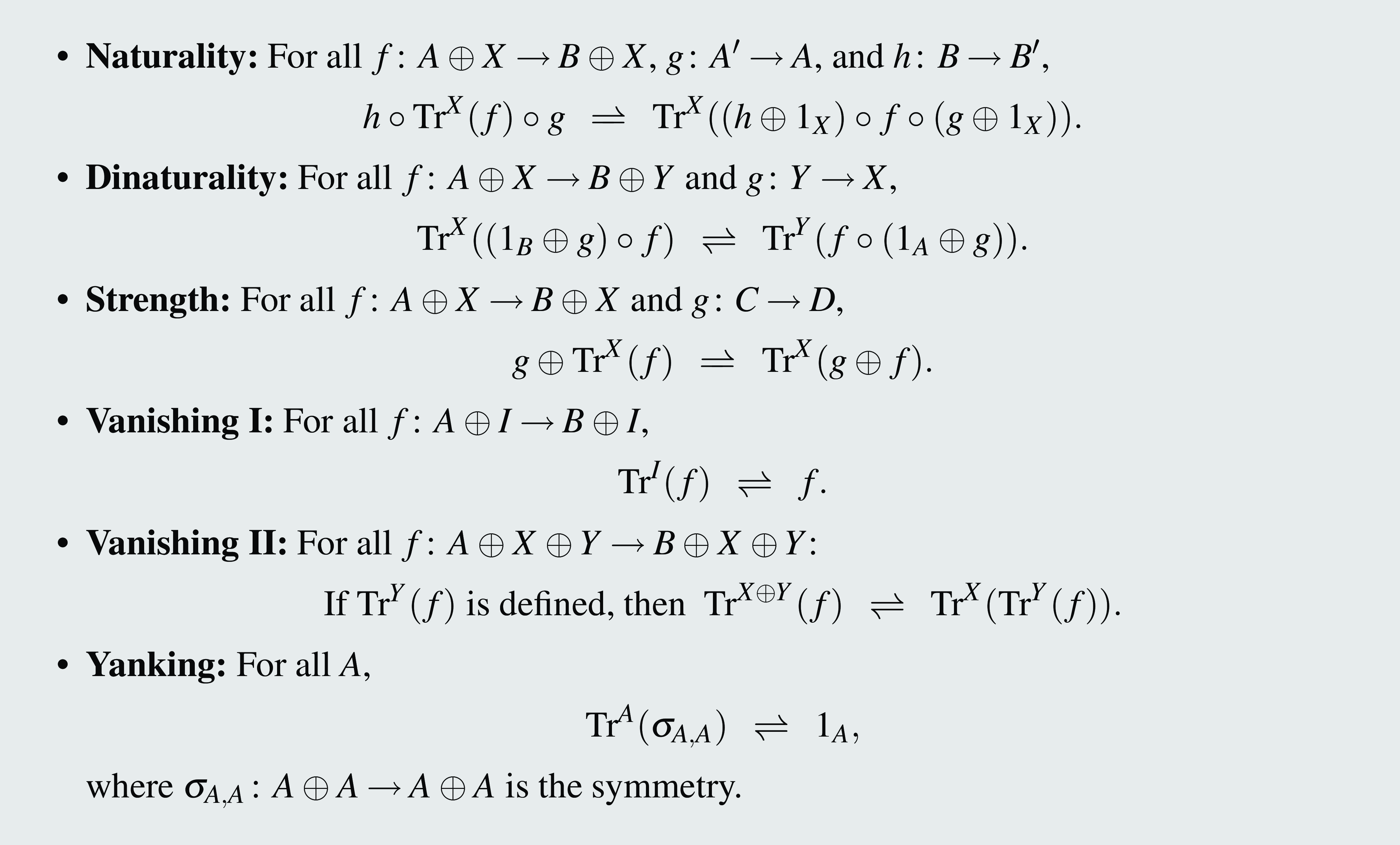


 Open access