


I. INTRODUCTION
With the advent of virtual and augmented reality comes the birth of a new medium: live captured three-dimensional (3D) content that can be experienced from any point of view. Such content ranges from static scans of compact 3D objects to dynamic captures of non-rigid objects such as people, to captures of rooms including furniture, public spaces swarming with people, and whole cities in motion. For such content to be captured at one place and delivered to another for consumption by a virtual or augmented reality device (or by more conventional means), the content needs to be represented and compressed for transmission or storage. Applications include gaming, tele-immersive communication, free navigation of highly produced entertainment as well as live events, historical artifact and site preservation, acquisition for special effects, and so forth. This paper presents a novel means of representing and compressing the visual part of such content.
Until this point, two of the more promising approaches to representing both static and time-varying 3D scenes have been polygonal meshes and point clouds, along with their associated color information. However, both approaches have drawbacks. Polygonal meshes represent surfaces very well, but they are not robust to noise and other structures typically found in live captures, such as lines, points, and ragged boundaries that violate the assumptions of a smooth surface manifold. Point clouds, on the other hand, have a hard time modeling surfaces as compactly as meshes.
We propose a hybrid between polygonal meshes and point clouds: polygon clouds. Polygon clouds are sets of polygons, often called a polygon soup. The polygons in a polygon cloud are not required to represent a coherent surface. Like the points in a point cloud, the polygons in a polygon cloud can represent noisy, real-world geometry captures without any assumption of a smooth 2D manifold. In fact, any polygon in a polygon cloud can be collapsed into a point or line as a special case. The polygons may also overlap. On the other hand, the polygons in the cloud can also be stitched together into a watertight mesh if desired to represent a smooth surface. Thus polygon clouds generalize both point clouds and polygonal meshes.
For concreteness, we focus on triangles instead of arbitrary polygons, and we develop an encoder and decoder for sequences of triangle clouds. We assume a simple group of frames (GOF) model, where each GOF begins with an Intra (I) frame, also called a reference frame or a key frame, which is followed by a sequence of Predicted (P) frames, also called inter frames. The triangles are assumed to be consistent across frames. That is, the triangles' vertices are assumed to be tracked from one frame to the next. The trajectories of the vertices are not constrained. Thus the triangles may change from frame to frame in location, orientation, and proportion.
For geometry encoding, redundancy in the vertex trajectories is removed by a spatial orthogonal transform followed by temporal prediction, allowing low latency. For color encoding, the triangles in each frame are projected back to the coordinate system of the reference frame. In the reference frame the triangles are voxelized in order to ensure that their color textures are sampled uniformly in space regardless of the sizes of the triangles, and in order to construct a common vector space in which to describe the color textures and their evolution from frame to frame. Redundancy of the color vectors is removed by a spatial orthogonal transform followed by temporal prediction, similar to redundancy removal for geometry. Uniform scalar quantization and entropy coding matched to the spatial transform are employed for both color and geometry.
We compare triangle clouds to both triangle meshes and point clouds in terms of compression, for live captured dynamic colored geometry. We find that triangle clouds can be compressed nearly as well as triangle meshes while being far more flexible in representing live captured content. We also find that triangle clouds can be used to compress point clouds with significantly better performance than previously demonstrated point cloud compression methods. Since we are motivated by virtual and augmented reality (VR/AR) applications, for which encoding and decoding have to have low latency, we focus on an approach that can be implemented at low computational complexity. A preliminary part of this work with more limited experimental evaluation was published in [Reference Pavez and Chou1].
The paper is organized as follows as follows. After a summary of related work in Section II, preliminary material is presented in Section III. Components of our compression system are described in Section IV, while the core of our system is given in Section V. Experimental results are presented in Section VI. The conclusion is in Section VII.
II. RELATED WORK
A) Mesh compression
3D mesh compression has a rich history, particularly from the 1990s forward. Overviews may be found in [Reference Alliez, Gotsman, Dodgson, Floater and Sabin2–Reference Peng, Kim and Jay Kuo4]. Fundamental is the need to code mesh topology, or connectivity, such as in [Reference Mamou, Zaharia and Prêteux5,Reference Rossignac6]. Beyond coding connectivity, coding the geometry, i.e., the positions of the vertices is also important. Many approaches have been taken, but one significant and practical approach to geometry coding is based on “geometry images” [Reference Gu, Gortler and Hoppe7] and their temporal extension, “geometry videos” [Reference Briceño, Sander, McMillan, Gortler and Hoppe8,Reference Collet9]. In these approaches, the mesh is partitioned into patches, the patches are projected onto a 2D plane as charts, non-overlapping charts are laid out in a rectangular atlas, and the atlas is compressed using a standard image or video coder, compressing both the geometry and the texture (i.e., color) data. For dynamic geometry, the meshes are assumed to be temporally consistent (i.e., connectivity is constant frame-to-frame) and the patches are likewise temporally consistent. Geometry videos have been used for representing and compressing free-viewpoint video of human actors [Reference Collet9]. Key papers on mesh compression of human actors in the context of tele-immersion include [Reference Doumanoglou, Alexiadis, Zarpalas and Daras10,Reference Mekuria, Sanna, Izquierdo, Bulterman and Cesar11].
B) Motion estimation
A critical part of dynamic mesh compression is the ability to track points over time. If a mesh is defined for a keyframe, and the vertices are tracked over subsequent frames, then the mesh becomes a temporally consistent dynamic mesh. There is a huge body of literature in the 3D tracking, 3D motion estimation or scene flow, 3D interest point detection and matching, 3D correspondence, non-rigid registration, and the like. We are particularly influenced by [Reference Dou12–Reference Newcombe, Fox and Seitz14], all of which produce in real time, given data from one or more RGBD sensors for every frame t, a parameterized mapping  $f_{\theta _t}:{\open R}^3\rightarrow {\open R}^3$ that maps points in frame t to points in frame t+1. Though corrections may need to be made at each frame, chaining the mappings together over time yields trajectories for any given set of points. Compressing these trajectories is similar to compressing motion capture (mocap) trajectories, which has been well studied. [Reference Hou, Chau, Magnenat-Thalmann and He15] is a recent example with many references. Compression typically involves an intra-frame transform to remove spatial redundancy and either temporal prediction (if low latency is required) or a temporal transform (if the entire clip or GOF is available) to remove temporal redundancy, as in [Reference Hou, Chau, Magnenat-Thalmann and He16].
C) Graph signal processing
Graph Signal Processing (GSP) has emerged as an extension of the theory of linear shift invariant signal processing to the processing of signals on discrete graphs, where the shift operator is taken to be the adjacency matrix of the graph, or alternatively the Laplacian matrix of the graph [Reference Sandryhaila and Moura17,Reference Shuman, Narang, Frossard, Ortega and Vandergheynst18]. Critically sampled perfect reconstruction wavelet filter banks on graphs were proposed in [Reference Narang and Ortega19,Reference Narang and Ortega20]. These constructions were used for dynamic mesh compression in [Reference Anis, Chou and Ortega21,Reference Nguyen, Chou and Chen22]. In particular [Reference Anis, Chou and Ortega21], simultaneously modifies the point cloud and fits triangular meshes. These meshes are time consistent, and come at different levels of resolution, which are used for multi-resolution transform coding of motion trajectories and color.
D) Point cloud compression using octrees
Sparse Voxel Octrees (SVOs) were developed in the 1980s to represent the geometry of 3D objects [Reference Jackins and Tanimoto23,Reference Meagher24]. Recently SVOs have been shown to have highly efficient implementations suitable for encoding at video frame rates [Reference Loop, Zhang and Zhang25]. In the guise of occupancy grids, they have also had significant use in robotics [Reference Elfes26–Reference Pathak, Birk, Poppinga and Schwertfeger28]. Octrees were first used for point cloud compression in [Reference Schnabel and Klein29]. They were further developed for progressive point cloud coding, including color attribute compression, in [Reference Huang, Peng, Kuo and Gopi30]. Octrees were extended to the coding of dynamic point clouds (i.e., point cloud sequences) in [Reference Kammerl, Blodow, Rusu, Gedikli, Beetz and Steinbach31]. The focus of [Reference Kammerl, Blodow, Rusu, Gedikli, Beetz and Steinbach31] was geometry coding; their color attribute coding remained rudimentary. Their method of inter-frame geometry coding was to take the exclusive-OR (XOR) between frames and code the XOR using an octree. Their method was implemented in the Point Cloud Library [Reference Rusu and Cousins32].
E) Color attribute compression for static point clouds
To better compress the color attributes in static voxelized point clouds, Zhang et al. used transform coding based on the Graph Fourier Transform (GFT), recently proposed in the context of GSP [Reference Zhang, Florêncio and Loop33]. While transform coding based on the GFT has good compression performance, it requires eigen-decompositions for each coded block, and hence may not be computationally attractive. To improve the computational efficiency, while not sacrificing compression performance, Queiroz and Chou developed an orthogonal Region-Adaptive Hierarchical Transform (RAHT) along with an entropy coder [Reference de Queiroz and Chou34]. RAHT is essentially a Haar transform with the coefficients appropriately weighted to take the non-uniform shape of the domain (or region) into account. As its structure matches the SVO, it is extremely fast to compute. Other approaches to non-uniform regions include the shape-adaptive discrete cosine transform [Reference Cohen, Tian and Vetro35] and color palette coding [Reference Dado, Kol, Bauszat, Thiery and Eisemann36]. Further approaches based on a non-uniform sampling of an underlying stationary process can be found in [Reference de Queiroz and Chou37], which uses the Karhunen–Loève transform matched to the sample, and in [Reference Hou, Chau, He and Chou38], which uses sparse representation and orthogonal matching pursuit.
F) Dynamic point cloud compression
Thanou et al. [Reference Thanou, Chou and Frossard39,Reference Thanou, Chou and Frossard40] were the first to deal fully with dynamic voxelized points clouds, by finding matches between points in adjacent frames, warping the previous frame to the current frame, predicting the color attributes of the current frame from the quantized colors of the previous frame, and coding the residual using the GFT-based method of [Reference Zhang, Florêncio and Loop33]. Thanou et al. used the XOR-based method of Kammerl et al. [Reference Kammerl, Blodow, Rusu, Gedikli, Beetz and Steinbach31] for inter-frame geometry compression. However, the method of [Reference Kammerl, Blodow, Rusu, Gedikli, Beetz and Steinbach31] proved to be inefficient, in a rate-distortion sense, for anything except slowly moving subjects, for two reasons. First, the method “predicts” the current frame from the previous frame, without any motion compensation. Second, the method codes the geometry losslessly, and so has no ability to perform a rate-distortion trade-off. To address these shortcomings, Queiroz and Chou [Reference de Queiroz and Chou41] used block-based motion compensation and rate-distortion optimization to select between coding modes (intra or motion-compensated coding) for each block. Further, they applied RAHT to coding the color attributes (in intra-frame mode), color prediction residuals (in inter-frame mode), and the motion vectors (in inter-frame mode). They also used in-loop deblocking filters. Mekuria et al. [Reference Mekuria, Blom and Cesar42] independently proposed block-based motion compensation for dynamic point cloud sequences. Although they did not use rate-distortion optimization, they used affine transformations for each motion-compensated block, rather than just translations. Unfortunately, it appears that block-based motion compensation of dynamic point cloud geometry tends to produce gaps between blocks, which are perceptually more damaging than indicated by objective metrics such as the Haussdorf-based metrics commonly used in geometry compression [Reference Mekuria, Li, Tulvan and Chou43].
G) Key learnings
Some of the key learnings from the previous work, taken as a whole, are that
• Point clouds are preferable to meshes for resilience to noise and non-manifold signals measured in real-world signals, especially for real-time capture where the computational cost of heavy duty pre-processing (e.g., surface reconstruction, topological denoising, charting) can be prohibitive.
• For geometry coding in static scenes, point clouds appear to be more compressible than meshes, even though the performance of point cloud geometry coding seems to be limited by the lossless nature of the current octree methods. In addition, octree processing for geometry coding is extremely fast.
• For color attribute coding in static scenes, both point clouds and meshes appear to be well compressible. If charting is possible, compressing the color as an image may win out due to the maturity of image compression algorithms today. However, direct octree processing for color attribute coding is extremely fast, as it is for geometry coding.
• For both geometry and color attribute coding in dynamic scenes (or inter-frame coding), temporally consistent dynamic meshes are highly compressible. However, finding a temporally consistent mesh can be challenging from a topological point of view as well as from a computational point of view.
In this work, we aim to achieve the high compression efficiency possible with the intra-frame point cloud compression and inter-frame dynamic mesh compression, while simultaneously achieving the high computational efficiency possible with octree-based processing, as well as its robustness to real-world noise and non-manifold data. We attain higher computational efficiency for temporal coding, by first exploiting available motion information for inter-frame prediction, instead of performing motion estimation at the encoder side as in [Reference Anis, Chou and Ortega21,Reference Thanou, Chou and Frossard39,Reference Thanou, Chou and Frossard40]. In practice, motion trajectories can be obtained in real time using several existing approaches [Reference Dou12–Reference Newcombe, Fox and Seitz14]. Second, for efficient and low complexity transform coding, we follow [Reference de Queiroz and Chou34].
H) Contributions and main results
Our contributions, which are summarized in more detail in Section VII, include
(i) Introduction of triangle clouds, a representation intermediate between triangle meshes and point clouds, for efficient compression as well as robustness to real-world data.
(ii) A comprehensive algorithm for triangle cloud compression, employing novel geometry, color, and temporal coding.
(iii) Reduction of inter- and intra-coding of color and geometry to compression of point clouds with different attributes.
(iv) Implementation of a low complexity point cloud transform coding system suitable for real time applications, including a new fast implementation of the transform from [Reference de Queiroz and Chou34].
We demonstrate the advantages of polygon clouds for compression throughout the extensive coding experiments evaluated using a variety of distortion measures. Our main findings are summarized as follows:
• Our intra-frame geometry coding is more efficient than previous intra-frame geometry coding based on point clouds by 5–10x or more in geometry bitrate,
• Our inter-frame geometry coding is better than our intra-frame geometry coding by 3x or more in geometry bitrate,
• Our inter-frame color coding is better than our/previous intra-frame color coding by up to 30% in color bitrate,
• Our temporal geometry coding is better than recent dynamic mesh compression by 6x in geometry bitrate, and
• Our temporal coding is better than recent point cloud compression by 33% in overall bitrate.
Our results also reveal the hyper-sensitivity of color distortion measures to geometry compression.
III. PRELIMINARIES

B) Dynamic triangle clouds
A dynamic triangle cloud is a numerical representation of a time changing 3D scene or object. We denote it by a sequence  $\lbrace {\cal T}^{(t)} \rbrace $ where ${\cal T}^{(t)}$ is a triangle cloud at time t. Each frame ${\cal T}^{(t)}$ is composed of a set of vertices ${\cal V}^{(t)}$, faces (polygons) ${\cal F}^{(t)}$, and color ${\cal C}^{(t)}$.
The geometry information (shape and position) consists of a list of vertices  ${\cal V}^{(t)}=\lbrace v_i^{(t)} : i=1,\,\ldots ,\, N_p\rbrace $, where each vertex $v_i^{(t)}=[x_i^{(t)},\,y_i^{(t)},\,z_i^{(t)}]$ is a point in 3D, and a list of triangles (or faces) ${\cal F}^{(t)}=\lbrace f_m^{(t)}: m=1,\,\ldots ,\,N_f \rbrace $, where each face $f_m^{(t)}=[i_m^{(t)},\,j_m^{(t)},\,k_m^{(t)}]$ is a vector of indices of vertices from ${\cal V}^{(t)}$. We denote by ${\bf V}^{(t)}$ the $N_p \times 3$ matrix whose i-th row is the point $v_i^{(t)}$, and similarly, we denote by ${\bf F}^{(t)}$ the $N_f \times 3$ matrix whose m-th row is the triangle $f_m^{(t)}$. The triangles in a triangle cloud do not have to be adjacent or form a mesh, and they can overlap. Two or more vertices of a triangle may have the same coordinates, thus collapsing into a line or point.
The color information consists of a list of colors  ${\cal C}^{(t)}=\lbrace c_n^{(t)} : n=1,\,\ldots ,\, N_c\rbrace $, where each color $c_n^{(t)}=[Y_n^{(t)},\,U_n^{(t)}$, $V_n^{(t)}]$ is a vector in YUV space (or other convenient color space). We denote by ${\bf C}^{(t)}$ the $N_c \times 3$ matrix whose n-th row is the color $c_n^{(t)}$. The list of colors represents the colors across the surfaces of the triangles. To be specific, $c_n^{(t)}$ is the color of a “refined” vertex $v_r^{(t)}(n)$, where the refined vertices are obtained by uniformly subdividing each triangle in ${\cal F}^{(t)}$ by upsampling factor U, as shown in Fig. 1(b) for U=4. We denote by ${\bf V}_r^{(t)}$ the $N_c \times 3$ matrix whose n-th row is the refined vertex $v_r^{(t)}(n)$. ${\bf V}_r^{(t)}$ can be computed from ${\cal V}^{(t)}$ and ${\cal F}^{(t)}$, so we do not need to encode it, but we will use it to compress the color information. Thus frame t of the triangle cloud can be represented by the triple ${\cal T}^{(t)}=({\bf V}^{(t)},{\bf F}^{(t)},{\bf C}^{(t)})$.
Triangle cloud geometry information. (b) A triangle in a dynamic triangle cloud is depicted. The vertices of the triangle at time t are denoted by 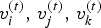 $v_i^{(t)},\,v_j^{(t)},\,v_k^{(t)}$. Colored dots represent “refined” vertices, whose coordinates can be computed from the triangle's coordinates using Alg. 5. Each refined vertex has a color attribute. (a) Man mesh. (b) Correspondences between two consecutive frames.
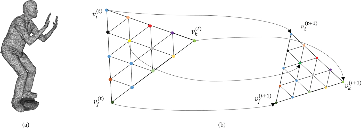
Note that a triangle cloud can be equivalently represented by a point cloud given by the refined vertices and the color attributes  $({\bf V}_r^{(t)}$, ${\bf C}^{(t)})$. For each triangle in the triangle cloud, there are $(U+1)(U+2)/2$ color values distributed uniformly on the triangle surface, with coordinates given by the refined vertices (see Fig. 1(b)). Hence the equivalent point cloud has $N_c = N_f(U+1)(U+2)/2$ points. We will make use of this point cloud representation property in our compression system. The up-sampling factor U should be high enough so that it does not limit the color spatial resolution obtainable by the color cameras. In our experiments, we set U=10 or higher. Setting U higher does not typically affect the bit rate significantly, though it does affect memory and computation in the encoder and decoder. Moreover, for U=10, the number of triangles is much smaller than the number of refined vertices ( $N_f \ll N_c$), which is one of the reasons we can achieve better geometry compression using a triangle cloud representation instead of a point cloud.
C) Compression system overview
In this section, we provide an overview of our system for compressing dynamic triangle clouds. We use a GOF model, in which the sequence is partitioned into GOFs. The GOFs are processed independently. Without loss of generality, we label the frames in a GOF  $t=1\ldots ,\,N$. There are two types of frames: reference and predicted. In each GOF, the first frame (t=1) is a reference frame and all other frames ( $t=2,\,\ldots ,\,N$) are predicted. Within a GOF, all frames must have the same number of vertices, triangles, and colors: $\forall t\in [N]$, ${\bf V}^{(t)} \in {\open R}^{N_p\times 3}$, ${\bf F}^{(t)} \in [N_p]^{N_f \times 3}$ and ${\bf C}^{(t)} \in {\open R}^{N_c \times 3}$. The triangles are assumed to be consistent across frames so that there is a correspondence between colors and vertices within the GOF. In Fig. 1(b), we show an example of the correspondences between two consecutive frames in a GOF. Different GOFs may have different numbers of frames, vertices, triangles, and colors.
We compress consecutive GOFs sequentially and independently, so we focus on the system for compressing an individual GOF  $({\bf V}^{(t)},\,{\bf F}^{(t)},\,{\bf C}^{(t)})$ for $t \in [N]$. The overall system is shown in Fig. 2, where ${\bf C}^{(t)}$ is known as ${\bf C}_r^{(t)}$ for reasons to be discussed later.
Encoder (left) and decoder (right). The switches are in the t=1 position, and flip for t>1.
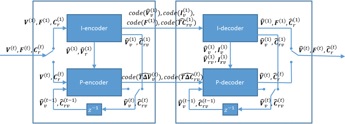
For all frames, our system first encodes geometry, i.e. vertices and faces, and then color. The color compression depends on the decoded geometry, as it uses a transform that reduces spatial redundancy.
For the reference frame at t=1, also known as the intra (I) frame, the I-encoder represents the vertices  ${\bf V}^{(1)}$ using voxels. The voxelized vertices ${\bf V}_v^{(1)}$ are encoded using an octree. The connectivity ${\bf F}^{(1)}$ is compressed without a loss using an entropy coder. The connectivity is coded only once per GOF since it is consistent across the GOF, i.e., ${\bf F}^{(t)}={\bf F}^{(1)}$ for $t\in [N]$. The decoded vertices $\hat {{\bf V}}^{(1)}$ are refined and used to construct an auxiliary point cloud $(\hat {{\bf V}}_r^{(1)},\,{\bf C}_r^{(1)})$. This point cloud is voxelized as $(\hat {{\bf V}}_{rv}^{(1)},\,{\bf C}_{rv}^{(1)})$, and its color attributes are then coded as $\widehat {{\bf TC}}_{rv}^{(1)}$ using the region adaptive hierarchical transform (RAHT) [Reference de Queiroz and Chou34], uniform scalar quantization, and adaptive Run-Length Golomb-Rice (RLGR) entropy coding [Reference Malvar44]. Here, ${\bf T}$ denotes the transform and hat denotes a quantity that has been compressed and decompressed. At the cost of additional complexity, the RAHT transform could be replaced by transforms with higher performance [Reference de Queiroz and Chou37,Reference Hou, Chau, He and Chou38].
For predicted (P) frames at t>1, the P-encoder computes prediction residuals from the previously decoded frame. Specifically, for each t>1 it computes a motion residual  $\Delta {\bf V}_v^{(t)}={\bf V}_v^{(t)}-\hat {{\bf V}}_v^{(t-1)}$ and a color residual $\Delta {\bf C}_{rv}^{(t)}={\bf C}_{rv}^{(t)}-\hat {{\bf C}}_{rv}^{(t-1)}$. These residuals are attributes of the following auxiliary point clouds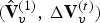 $(\hat {{\bf V}}_v^{(1)},\,\Delta {\bf V}_v^{(t)})$,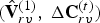 $(\hat {{\bf V}}_{rv}^{(1)},\,\Delta {\bf C}_{rv}^{(t)})$, respectively. Then transform coding is applied using again the RAHT followed by uniform scalar quantization and entropy coding.
It is important to note that we do not directly compress the list of vertices  ${\bf V}^{(t)}$ or the list of colors ${\bf C}^{(t)}$ (or their prediction residuals). Rather, we voxelize them first with respect to their corresponding vertices in the reference frame, and then compress them. This ensures that (1) if two or more vertices or colors fall into the same voxel, they receive the same representation and hence are encoded only once, and (2) the colors (on the set of refined vertices) are resampled uniformly in space regardless of the density, size or shapes of triangles.
In the next section, we detail the basic elements of the system: refinement, voxelization, octrees, and transform coding. Then, in Section V, we detail how these basic elements are put together to encode and decode a sequence of triangle clouds.
IV. REFINEMENT, VOXELIZATION, OCTREES, AND TRANSFORM CODING
In this section, we introduce the most important building blocks of our compression system. We describe their efficient implementations, with detailed pseudo code that can be found in the Appendix.
A) Refinement
A refinement refers to a procedure for dividing the triangles in a triangle cloud into smaller (equal sized) triangles. Given a list of triangles  ${\bf F}$, its corresponding list of vertices ${\bf V}$, and upsampling factor U, a list of “refined” vertices ${\bf V}_r$ can be produced using Algorithm 5. Step 1 (in Matlab notation) assembles three equal-length lists of vertices (each as an $N_f\times 3$ matrix), containing the three vertices of every face. Step 5 appends linear combinations of the faces' vertices to a growing list of refined vertices. Note that since the triangles are independent, the refinement can be implemented in parallel. We assume that the refined vertices in ${\bf V}_r$ can be colored, such that the list of colors ${\bf C}$ is in 1-1 correspondence with the list of refined vertices ${\bf V}_r$. An example with a single triangle is depicted in Fig. 1(b), where the colored dots correspond to refined vertices.
B) Morton codes and voxelization
A voxel is a volumetric element used to represent the attributes of an object in 3D over a small region of space. Analogous to 2D pixels, 3D voxels are defined on a uniform grid. We assume the geometric data live in the unit cube  $[0,\,1)^3$, and we partition the cube uniformly into voxels of size $2^{-J} \times 2^{-J} \times 2^{-J}$.
Now consider a list of points  ${\bf V}=[v_i]$ and an equal-length list of attributes ${\bf A}=[a_i]$, where $a_i$ is the real-valued attribute (or vector of attributes) of $v_i$. (These may be, for example, the list of refined vertices ${\bf V}_r$ and their associated colors ${\bf C}_r={\bf C}$ as discussed above.) In the process of voxelization, the points are partitioned into voxels, and the attributes associated with the points in a voxel are averaged. The points within each voxel are quantized to the voxel center. Each occupied voxel is then represented by the voxel center and the average of the attributes of the points in the voxel. Moreover, the occupied voxels are put into Z-scan order, also known as Morton order [Reference Morton45]. The first step in voxelization is to quantize the vertices and to produce their Morton codes. The Morton code m for a point $(x,\,y,\,z)$ is obtained simply by interleaving (or “swizzling”) the bits of x, y, and z, with x being higher order than y, and y being higher order than z. For example, if $x=x_4x_2x_1$, $y=y_4y_2y_1$, and $z=z_4z_2z_1$ (written in binary), then the Morton code for the point would be $m=x_4y_4z_4x_2y_2z_2x_1y_1z_1$. The Morton codes are sorted, duplicates are removed, and all attributes whose vertices have a particular Morton code are averaged.
Voxelization (voxelize)

The procedure is detailed in Algorithm 1.  ${\bf V}_{int}$ is the list of vertices with their coordinates, previously in $[0,\,1)$, now mapped to integers in $\{0,\,\ldots ,\,2^J-1\}$. ${\bf M}$ is the corresponding list of Morton codes. ${\bf M}_v$ is the list of Morton codes, sorted with duplicates removed, using the Matlab function unique. ${\bf I}$ and ${\bf I}_v$ are vectors of indices such that ${\bf M}_v={\bf M}({\bf I})$ and ${\bf M}={\bf M}_v({\bf I}_v)$, in Matlab notation. (That is, the $i_v$th element of ${\bf M}_v$ is the ${\bf I}(i_v)$th element of ${\bf M}$ and the ith element of ${\bf M}$ is the ${\bf I}_v(i)$th element of ${\bf M}_v$.) ${\bf A}_v=[\bar a_j]$ is the list of attribute averages
 $$\bar{a}_j = \displaystyle{1 \over {N_j}}\sum\limits_{i:{\bf M}(i) = {\bf M}_v(j)} {a_i},$$
where  $N_j$ is the number of elements in the sum. ${\bf V}_v$ is the list of voxel centers. The complexity of voxelization is dominated by sorting of the Morton codes, thus the algorithm has complexity ${\cal O}(N\log N)$, where N is the number of input points.
C) Octree encoding
Any set of voxels in the unit cube, each of size  $2^{-J} \times 2^{-J} \times 2^{-J}\!$, designated occupied voxels, can be represented with an octree of depth J [Reference Jackins and Tanimoto23,Reference Meagher24]. An octree is a recursive subdivision of a cube into smaller cubes, as illustrated in Fig. 3. Cubes are subdivided only as long as they are occupied (i.e., contain any occupied voxels). This recursive subdivision can be represented by an octree with depth $J\!$, where the root corresponds to the unit cube. The leaves of the tree correspond to the set of occupied voxels.
Cube subdivision. Blue cubes represent occupied regions of space.
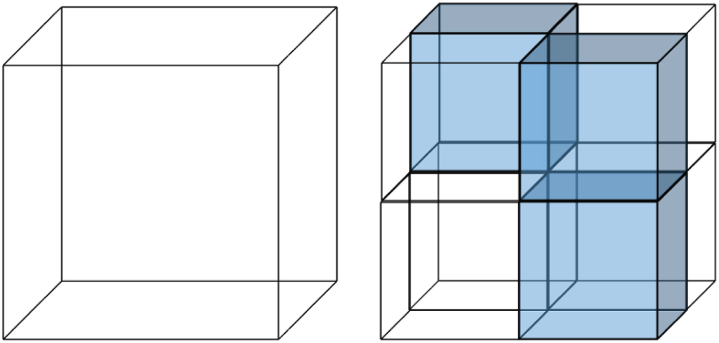
There is a close connection between octrees and Morton codes. In fact, the Morton code of a voxel, which has length  $3\,J$ bits broken into J binary triples, encodes the path in the octree from the root to the leaf containing the voxel. Moreover, the sorted list of Morton codes results from a depth-first traversal of the tree.
Each internal node of the tree can be represented by one byte, to indicate which of its eight children are occupied. If these bytes are serialized in a depth-first traversal of the tree, the serialization (which has a length in bytes equal to the number of internal nodes of the tree) can be used as a description of the octree, from which the octree can be reconstructed. Hence the description can also be used to encode the ordered list of Morton codes of the leaves. This description can be further compressed using a context adaptive arithmetic encoder. However, for simplicity, in our experiments, we use gzip instead of an arithmetic encoder.
In this way, we encode any set of occupied voxels in a canonical (Morton) order.
D) Transform coding
In this section, we describe the RAHT [Reference de Queiroz and Chou34] and its efficient implementation. RAHT is a sequence of orthonormal transforms applied to attribute data living on the leaves of an octree. For simplicity, we assume the attributes are scalars. This transform processes voxelized attributes in a bottom-up fashion, starting at the leaves of the octree. The inverse transform reverses this order.
Consider eight adjacent voxels, three of which are occupied, having the same parent in the octree, as shown in Fig. 4. The colored voxels are occupied (have an attribute) and the transparent ones are empty. Each occupied voxel is assigned a unit weight. For the forward transform, transformed attribute values and weights will be propagated up the tree.
One level of RAHT applied to a cube of eight voxels, three of which are occupied.
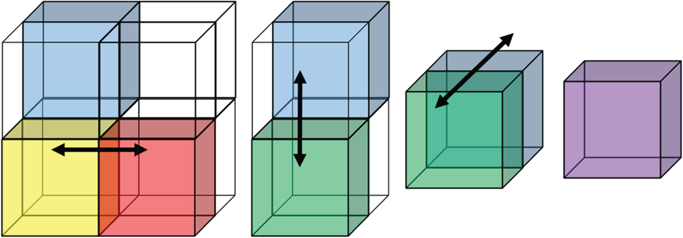
One level of the forward transform proceeds as follows. Pick a direction (x, y, or z), then check whether there are two occupied cubes that can be processed along that direction. In the leftmost part of Fig. 4 there are only three occupied cubes, red, yellow, and blue, having weights  $w_{r}$, $w_{y}$, and $w_{b}$, respectively. To process in the direction of the x-axis, since the blue cube does not have a neighbor along the horizontal direction, we copy its attribute value $a_b$ to the second stage and keep its weight $w_{b}$. The attribute values $a_y$ and $a_r$ of the yellow and red cubes can be processed together using the orthonormal transformation
 $$\left[ {\matrix{ {a_g^0 } \cr {{\rm }a_g^1 } \cr } } \right] = \displaystyle{1 \over {\sqrt {w_y + w_r} }}\left[ {\matrix{ {\sqrt {w_y} } & {\sqrt {w_r} } \cr {{\rm }-\sqrt {w_r} } & {\sqrt {w_y} } \cr } } \right]\left[ {\matrix{ {a_y} \cr {a_r} \cr } } \right],$$
where the transformed coefficients  $a_g^0$ and $a_g^1$, respectively, represent low pass and high pass coefficients appropriately weighted. Both transform coefficients now represent information from a region with weight $w_g=w_y+w_r$ (green cube). The high pass coefficient is stored for entropy coding along with its weight, while the low pass coefficient is further processed and put in the green cube. For processing along the y-axis, the green and blue cubes do not have neighbors, so their values are copied to the next level. Then we process in the z direction using the same transformation in (2) with weights $w_g$ and $w_b$.
This process is repeated for each cube of eight subcubes at each level of the octree. After J levels, there remains one low pass coefficient that corresponds to the DC component; the remainder are high pass coefficients. Since after each processing of a pair of coefficients, the weights are added and used during the next transformation, the weights can be interpreted as being inversely proportional to frequency. The DC coefficient is the one that has the largest weight, as it is processed more times and represents information from the entire cube, while the high pass coefficients, which are produced earlier, have smaller weights because they contain information from a smaller region. The weights depend only on the octree (not the coefficients themselves), and thus can provide a frequency ordering for the coefficients. We sort the transformed coefficients by decreasing the magnitude of weight.
Finally, the sorted coefficients are quantized using uniform scalar quantization, and are entropy coded using adaptive Run Length Golomb-Rice coding [Reference Malvar44]. The pipeline is illustrated in Fig. 5.
Transform coding system for voxelized point clouds.

Note that the RAHT has several properties that make it suitable for real-time compression. At each step, it applies several  $2 \times 2$ orthonormal transforms to pairs of voxels. By using the Morton ordering, the j-th step of the RAHT can be implemented with worst-case time complexity ${\cal O}({N}_{vox,j})$, where $N_{vox,j}$ is the number of occupied voxels of size $2^{-j} \times 2^{-j} \times 2^{-j}$. The overall complexity of the RAHT is ${\cal O}(J N_{vox,J})$. This can be further reduced by processing cubes in parallel. Note that within each GOF, only two different RAHTs will be applied multiple times. To encode motion residuals, a RAHT will be implemented using the voxelization with respect to the vertices of the reference frame. To encode color of the reference frame and color residuals of predicted frames, the RAHT is implemented with respect to the voxelization of the refined vertices of the reference frame.
Efficient implementations of RAHT and its inverse are detailed in Algorithms 3 and 4, respectively. Algorithm 2 is a prologue to each and needs to be run twice per GOF. For completeness we include in the Appendix our uniform scalar quantization in Algorithm 7.
Prologue to RAHT and its Inverse (IRAHT) (prologue)

Region Adaptive Hierarchical Transform

Inverse Region Adaptive Hierarchical Transform

V. ENCODING AND DECODING
In this section, we describe in detail encoding and decoding of dynamic triangle clouds. First we describe encoding and decoding of reference frames. Following that, we describe encoding and decoding of predicted frames. For both reference and predicted frames, we describe first how geometry is encoded and decoded, and then how color is encoded and decoded. The overall system is shown in Fig. 2.
A) Encoding and decoding of reference frames
For reference frames, encoding is summarized in Algorithm 8, while decoding is summarized in Algorithm 9, which can be found in the Appendix. For both reference and predicted frames, the geometry information is encoded and decoded first, since color processing depends on the decoded geometry.
1) Geometry encoding and decoding
We assume that the vertices in  ${\bf V}^{(1)}$ are in Morton order. If not, we put them into Morton order and permute the indices in ${\bf F}^{(1)}$ accordingly. The lists ${\bf V}^{(1)}$ and ${\bf F}^{(1)}$ are the geometry-related quantities in the reference frame transmitted from the encoder to the decoder. ${\bf V}^{(1)}$ will be reconstructed at the decoder with some loss as $\hat {{\bf V}}^{(1)}$, and ${\bf F}^{(1)}$ will be reconstructed losslessly. We now describe the process.
At the encoder, the vertices in  ${\bf V}^{(1)}$ are first quantized to the voxel grid, producing a list of quantized vertices $\hat {{\bf V}}^{(1)}$, the same length as ${\bf V}^{(1)}$. There may be duplicates in $\hat {{\bf V}}^{(1)}$, because some vertices may have collapsed to the same grid point. $\hat {{\bf V}}^{(1)}$ is then voxelized (without attributes), the effect of which is simply to remove the duplicates, producing a possibly slightly shorter list $\hat {{\bf V}}_v^{(1)}$ along with a list of indices ${\bf I}_v^{(1)}$ such that (in Matlab notation) $\hat {{\bf V}}^{(1)}=\hat {{\bf V}}_v^{(1)}({\bf I}_v^{(1)})$. Since $\hat {{\bf V}}_v^{(1)}$ has no duplicates, it represents a set of voxels. This set can be described by an octree. The byte sequence representing the octree can be compressed with any entropy encoder; we use gzip. The list of indices ${\bf I}_v^{(1)}$, which has the same length as $\hat {{\bf V}}^{(1)}$, indicates, essentially, how to restore the duplicates, which are missing from $\hat {{\bf V}}_v^{(1)}$. In fact, the indices in ${\bf I}_v^{(1)}$ increase in unit steps for all vertices in $\hat {{\bf V}}^{(1)}$ except the duplicates, for which there is no increase. The list of indices is thus a sequence of runs of unit increases alternating with runs of zero increases. This binary sequence of increases can be encoded with any entropy encoder; we use gzip on the run lengths. Finally, the list of faces ${\bf F}^{(1)}$ can be encoded with any entropy encoder; we again use gzip, though algorithms such as [Reference Mamou, Zaharia and Prêteux5,Reference Rossignac6] might also be used.
The decoder entropy decodes  $\hat {{\bf V}}_v^{(1)}$, ${\bf I}_v^{(1)}$, and ${\bf F}^{(1)}$, and then recovers $\hat {{\bf V}}^{(1)}=\hat {{\bf V}}_v^{(1)}({\bf I}_v^{(1)})$, which is the quantized version of ${\bf V}^{(1)}$, to obtain both $\hat {{\bf V}}^{(1)}$ and ${\bf F}^{(1)}$.
2) Color encoding and decoding
The RAHT, required for transform coding of the color signal, is constructed from an octree, or equivalently from a voxelized point cloud. We first describe how to construct such point set from the decoded geometry.
Let  ${\bf V}_r^{(1)}=refine({\bf V}^{(1)},\,{\bf F}^{(1)},\,U)$ be the list of “refined vertices” obtained by upsampling, by factor U, the faces ${\bf F}^{(1)}$ whose vertices are ${\bf V}^{(1)}$. We assume that the colors in the list ${\bf C}_r^{(1)}={\bf C}^{(1)}$ correspond to the refined vertices in ${\bf V}_r^{(1)}$. In particular, the lists have the same length. Here, we subscript the list of colors by an “r” to indicate that it corresponds to the list of refined vertices.
When the vertices  ${\bf V}^{(1)}$ are quantized to $\hat {{\bf V}}^{(1)}$, the refined vertices change to $\hat {{\bf V}}_r^{(1)}=refine(\hat {{\bf V}}^{(1)},\,{\bf F}^{(1)},\,U)$. The list of colors ${\bf C}_r^{(1)}$ can also be considered as indicating the colors on $\hat {{\bf V}}_r^{(1)}$. The list ${\bf C}_r^{(1)}$ is the color-related quantity in the reference frame transmitted from the encoder to the decoder. The decoder will reconstruct ${\bf C}_r^{(1)}$ with some loss $\hat {{\bf C}}_r^{(1)}$. We now describe the process.
At the encoder, the refined vertices  $\hat {{\bf V}}_r^{(1)}$ are obtained as described above. These vertices and the color information form a point cloud $(\hat {{\bf V}}_r^{(1)},\,{\bf C}_r^{(1)} )$, which will be voxelized and compressed as follows. The vertices $\hat {{\bf V}}_r^{(1)}$ and their associated color attributes ${\bf C}_r^{(1)}$ are voxelized using (1), to obtain a list of voxels $\hat {{\bf V}}_{rv}^{(1)}$, the list of voxel colors ${\bf C}_{rv}^{(1)}$, and the list of indices ${\bf I}_{rv}^{(1)}$ such that (in Matlab notation) $\hat {{\bf V}}_r^{(1)}=\hat {{\bf V}}_{rv}^{(1)}({\bf I}_{rv}^{(1)})$. The list of indices ${\bf I}_{rv}^{(1)}$ has the same length as $\hat {{\bf V}}_r^{(1)}$, and contains for each vertex in $\hat {{\bf V}}_r^{(1)}$ the index of its corresponding vertex in $\hat {{\bf V}}_{rv}^{(1)}$. Particularly, if the upsampling factor U is large, there may be many refined vertices falling into each voxel. Hence the list $\hat {{\bf V}}_{rv}^{(1)}$ may be significantly shorter than the list $\hat {{\bf V}}_r^{(1)}$ (and the list ${\bf I}_{rv}^{(1)}$). However, unlike the geometry case, in this case, the list ${\bf I}_{rv}^{(1)}$ need not be transmitted since it can be reconstructed from the decoded geometry.
The list of voxel colors  $\hat {{\bf C}}_{rv}^{(1)}$, each with unit weight (see Section IVD), is transformed by RAHT to an equal-length list of transformed colors ${\bf TC}_{rv}^{(1)}$ and associated weights ${\bf W}_{rv}^{(1)}$. The transformed colors are then uniformly quantized with stepsize $\Delta _{color,intra}$ to obtain $\widehat {{\bf TC}}_{rv}^{(1)}$. The quantized RAHT coefficients are entropy coded as described in Section IV using the associated weights, and are transmitted. Finally, $\widehat {{\bf TC}}_{rv}^{(1)}$ is inverse transformed by RAHT to obtain $\hat {{\bf C}}_{rv}^{(1)}$. These represent the quantized voxel colors, and will be used as a reference for subsequent predicted frames.
At the decoder, similarly, the refined vertices  $\hat {{\bf V}}_r^{(1)}$ are recovered from the decoded geometry information. First upsampling, by factor U, the faces ${\bf F}^{(1)}$ whose vertices are $\hat {{\bf V}}^{(1)}$ (both of which have been decoded already in the geometry step). $\hat {{\bf V}}_r^{(1)}$ is then voxelized (without attributes) to produce the list of voxels $\hat {{\bf V}}_{rv}^{(1)}$ and list of indices ${\bf I}_{rv}^{(1)}$ such that $\hat {{\bf V}}_r^{(1)}=\hat {{\bf V}}_{rv}^{(1)}({\bf I}_{rv}^{(1)})$. The weights ${\bf W}_{rv}^{(1)}$ are recovered by using RAHT to transform a null signal on the vertices $\hat {{\bf V}}_r^{(1)}$, each with unit weight. Then $\widehat {{\bf TC}}_{rv}^{(1)}$ is entropy decoded using the recovered weights and inverse transformed by RAHT to obtain the quantized voxel colors $\hat {{\bf C}}_{rv}^{(1)}$. Finally, the quantized refined vertex colors can be obtained as $\hat {{\bf C}}_r^{(1)}=\hat {{\bf C}}_{rv}^{(1)}({\bf I}_{rv}^{(1)})$.
B) Encoding and decoding of predicted frames
We assume that all N frames in a GOP are aligned. That is, the lists of faces,  ${\bf F}^{(1)},\,\ldots ,\,{\bf F}^{(N)}$, are all identical. Moreover, the lists of vertices, ${\bf V}^{(1)},\,\ldots ,\,{\bf V}^{(N)}$, all correspond in the sense that the ith vertex in list ${\bf V}^{(1)}$ (say, $v^{(1)}(i)=v_i^{(1)}$) corresponds to the ith vertex in list ${\bf V}^{(t)}$ (say, $v^{(t)}(i)=v_i^{(t)}$), for all $t=1,\,\ldots ,\,N$. $(v^{(1)}(i),\,\ldots ,\,v^{(N)}(i))$ is the trajectory of vertex i over the GOF, $i=1,\,\ldots ,\,N_p$, where $N_p$ is the number of vertices.
Similarly, when the faces are upsampled by factor U to create new lists of refined vertices,  ${\bf V}_r^{(1)},\,\ldots ,\,{\bf V}_r^{(N)}$ — and their colors, ${\bf C}_r^{(1)},\,\ldots ,\,{\bf C}_r^{(N)}$ — the $i_r$th elements of these lists also correspond to each other across the GOF, $i_r=1,\,\ldots ,\,N_c$, where $N_c$ is the number of refined vertices, or the number of colors.
The trajectory  $\{(v^{(1)}(i),\,\ldots ,\,v^{(N)}(i)):i=1,\,\ldots ,\,N_p\}$ can be considered an attribute of vertex $v^{(1)}(i)$, and likewise the trajectories $\{(v_r^{(1)}(i_r),\,\ldots ,\,v_r^{(N)}(i_r)):i_r=1,\,\ldots ,\,N_c\}$ and $\{(c_r^{(1)}(i_r),\,\ldots ,\,c_r^{(N)}(i_r)):i_r=1,\,\ldots ,\,N_c\}$ can be considered attributes of refined vertex $v_r^{(1)}(i_r)$. Thus the trajectories can be partitioned according to how the vertex $v^{(1)}(i)$ and the refined vertex $v_r^{(1)}(i_r)$ are voxelized. As for any attribute, the average of the trajectories in each cell of the partition is used to represent all trajectories in the cell. Our scheme codes these representative trajectories. This could be a problem if trajectories diverge from the same, or nearly the same, point, for example, when clapping hands separately. However, this situation is usually avoided by restarting the GOF by inserting a keyframe, or reference frame, whenever the topology changes, and by using a sufficiently fine voxel grid.
In this section, we show how to encode and decode the predicted frames, i.e., frames  $t=2,\,\ldots ,\,N$, in each GOF. The frames are processed one at a time, with no look-ahead, to minimize latency. The pseudo code can be found in the Appendix, the encoding is detailed in Algorithm 10, while decoding is detailed in Algorithm 11.
1) Geometry encoding and decoding
At the encoder, for frame t, as for frame 1, the vertices  ${\bf V}^{(1)}$, or equivalently the vertices $\hat {{\bf V}}^{(1)}$, are voxelized. However, for frame t>1 the voxelization occurs with attributes ${\bf V}^{(t)}$. In this sense, the vertices ${\bf V}^{(t)}$ are projected back to the reference frame, where they are voxelized like attributes. As for frame 1, this produces a possibly slightly shorter list $\hat {{\bf V}}_v^{(1)}$ along with a list of indices ${\bf I}_v^{(1)}$ such that $\hat {{\bf V}}^{(1)}=\hat {{\bf V}}_v^{(1)}({\bf I}_v^{(1)})$. In addition, it produces an equal-length list of representative attributes, ${\bf V}_v^{(t)}$. Such a list is produced every frame. Therefore, the previous frame can be used as a prediction. The prediction residual $\Delta {\bf V}_v^{(t)}={\bf V}_v^{(t)}-\hat {{\bf V}}_v^{(t-1)}$ is transformed, quantized with stepsize $\Delta _{motion}$, inverse transformed, and added to the prediction to obtain the reproduction $\hat {{\bf V}}_v^{(t)}$, which goes into the frame buffer. The quantized transform coefficients are entropy coded. We use adaptive RLGR as the entropy coder. In this process, the prediction residuals correspond to attributes of a point cloud given by the triangle's vertices at the reference frame. Note that the RAHT used to transform the prediction residual $\Delta {\bf V}_v^{(t)}$ is built using the voxelized point cloud at the reference frame $\hat {{\bf V}}_v^{(1)}$, which is different than the RAHT used for color coding.
At the decoder, the entropy code for the quantized transform coefficients of the prediction residual is received, entropy decoded, inverse transformed, inverse quantized, and added to the prediction to obtain  $\hat {{\bf V}}_v^{(t)}$, which goes into the frame buffer. Finally, $\hat {{\bf V}}^{(t)}=\hat {{\bf V}}_v^{(t)}({\bf I}_v^{(1)})$ is sent to the renderer.
2) Color encoding and decoding
At the encoder, for frame t>1, as for frame t=1, the refined vertices  $\hat {{\bf V}}_r^{(1)}$, are voxelized with attributes ${\bf C}_r^{(t)}$. In this sense, the colors ${\bf C}_r^{(t)}$ are projected back to the reference frame, where they are voxelized. As for frame t=1, this produces a significantly shorter list $\hat {{\bf V}}_{rv}^{(1)}$ along with a list of indices ${\bf I}_{rv}^{(1)}$ such that $\hat {{\bf V}}_r^{(1)}=\hat {{\bf V}}_{rv}^{(1)}({\bf I}_{rv}^{(1)})$. In addition, it produces a list of representative attributes, ${\bf C}_{rv}^{(t)}$. Such a list is produced every frame. Therefore the previous frame can be used as a prediction. The prediction residual $\Delta {\bf C}_{rv}^{(t)}={\bf C}_{rv}^{(t)}-\hat {{\bf C}}_{rv}^{(t-1)}$ is transformed, quantized with stepsize $\Delta _{color,inter}$, inverse transformed, and added to the prediction to obtain the reproduction $\hat {{\bf C}}_{rv}^{(t)}$, which goes into the frame buffer. The quantized transform coefficients are entropy coded. We use adaptive RLGR as the entropy coder.
At the decoder, the entropy code for the quantized transform coefficients of the prediction residual is received, entropy decoded, inverse transformed, inverse quantized, and added to the prediction to obtain  $\hat {{\bf C}}_{rv}^{(t)}$, which goes into the frame buffer. Finally, $\hat {{\bf C}}_r^{(t)}=\hat {{\bf C}}_{rv}^{(t)}({\bf I}_{rv}^{(1)})$ is sent to the renderer.
C) Rendering for visualization and distortion computation
The decompressed dynamic triangle cloud given by  $\lbrace \hat {{\bf V}}^{(t)},\,\hat {{\bf C}}_r^{(t)},\,{\bf F}^{(t)}\rbrace _{t=1}^N$ may have varying density across triangles resulting in some holes or transparent looking regions, which are not satisfactory for visualization. We apply the triangle refinement function on the set of vertices and faces from Algorithm 5 and produce the redundant representation $\lbrace \hat {{\bf V}}_r^{(t)},\,\hat {{\bf C}}_r^{(t)},\,{\bf F}_r^{(t)}\rbrace _{t=1}^N$. This sequence consists of a dynamic point cloud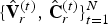 $\lbrace \hat {{\bf V}}_r^{(t)},\,\hat {{\bf C}}_r^{(t)}\rbrace _{t=1}^N$, whose colored points lie in the surfaces of triangles given by $\lbrace \hat {{\bf V}}_r^{(t)},\,{\bf F}_r^{(t)}\rbrace _{t=1}^N$. This representation is further refined using a similar method to increase the spatial resolution by adding a linear interpolation function for the color attributes as shown in Algorithm 6. The output is a denser point cloud, denoted by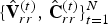 $\lbrace \hat {{\bf V}}_{rr}^{(t)},\,\hat {{\bf C}}_{rr}^{(t)}\rbrace _{t=1}^N$. We use this denser point cloud for visualization and distortion computation in the experiments described in the next section.
VI. EXPERIMENTS
In this section, we evaluate the RD performance of our system, for both intra-frame and inter-frame coding, for both color and geometry, under a variety of different error metrics. Our baseline for comparison to previous work is the intra-frame coding of colored voxels using octree coding for geometry [Reference Meagher24,Reference Schnabel and Klein29,Reference Kammerl, Blodow, Rusu, Gedikli, Beetz and Steinbach31,Reference Ochotta and Saupe46] and RAHT coding for colors [Reference de Queiroz and Chou34].
A) Dataset
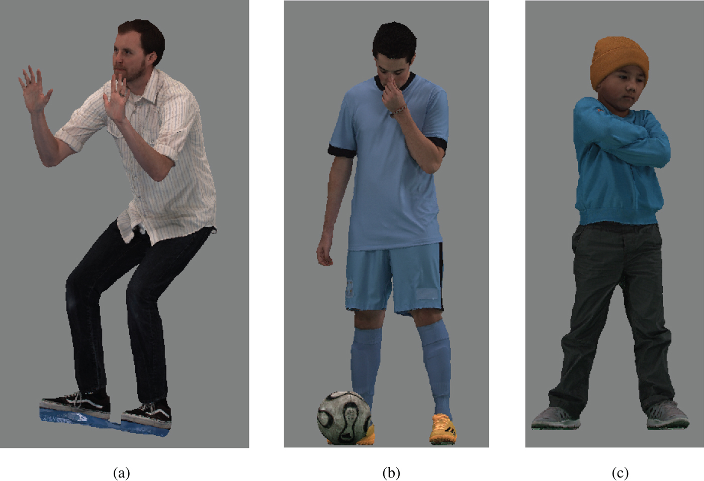
We use triangle cloud sequences derived from the Microsoft HoloLens Capture (HCap) mesh sequences Man, Soccer, and Breakers.Footnote 1 The initial frame from each sequence is shown in Figs 6a–c. In the HCap sequences, each frame is a triangular mesh. The frames are partitioned into GOFs. Within each GOF, the meshes are consistent, i.e., the connectivity is fixed but the positions of the triangle vertices evolve in time. We construct a triangle cloud from each mesh at time t as follows. For the vertex list  ${\bf V}^{(t)}$ and face list ${\bf F}^{(t)}$, we use the vertex and face lists directly from the mesh. For the color list ${\bf C}^{(t)}$, we upsample each face by factor U=10 to create a list of refined vertices, and then sample the mesh's texture map at the refined vertices. The geometric data are scaled to fit in the unit cube $[0,\,1]^3$. Our voxel size is $2^{-J}\times 2^{-J}\times 2^{-J}$, where J=10 is the maximum depth of the octree. All sequences are 30 frames per second. The overall statistics are described in Table 2.
Initial frames of datasets Man, Soccer, and Breakers. (a) Man. (b) Soccer. (c) Breakers.
Dataset statistics. Number of frames, number of GOFs (i.e., number of reference frames), and average number of vertices and faces per reference frame, in the original HCap datasets, and average number of occupied voxels per frame after voxelization with respect to reference frames. All sequences are 30 fps. For voxelization, all HCap meshes were upsampled by a factor of U=10, normalized to a  $1\times 1\times 1$ bounding cube, and then voxelized into voxels of size $2^{-J}\times 2^{-J}\times 2^{-J}$, J=10

B) Distortion metrics
Comparing algorithms for compressing colored 3D geometry poses some challenges because there is no single agreed upon metric or distortion measure for this type of data. Even if one attempts to separate the photometric and geometric aspects of distortion, there is often an interaction between the two. We consider several metrics for both color and geometry to evaluate different aspects of our compression system.
1) Projection distortion
One common approach to evaluating the distortion of compressed colored geometry relative to an original is to render both the original and compressed versions of the colored geometry from a particular point of view, and compare the rendered images using a standard image distortion measure such as peak signal-to-noise ratio (PSNR).
One question that arises with this approach is which viewpoint, or set of viewpoints, should be used. Another question is which method of rendering should be used. We choose to render from six viewpoints, by voxelizing the colored geometry of the refined and interpolated dynamic point cloud 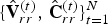 $\lbrace \hat {{\bf V}}_{rr}^{(t)},\,\hat {{\bf C}}_{rr}^{(t)}\rbrace _{t=1}^N$ described in Section VC, and projecting the voxels onto the six faces of the bounding cube, using orthogonal projection. For a cube of size $2^J\times 2^J\times 2^J$ voxels, the voxelized object is projected onto six images each of size $2^J\times 2^J$ pixels. If multiple occupied voxels project to the same pixel on a face, then the pixel takes the color of the occupied voxel closest to the face, i.e., hidden voxels are removed. If no occupied voxels project to a pixel on a face, then the pixel takes a neutral gray color. The mean squared error over the six faces and over the sequence is reported as PSNR separately for each color component: Y, U, and V. We call this the projection distortion. The projection distortion measures color distortion directly, but it also measures geometry distortion indirectly. Thus we will report the projection distortion as a function of the motion stepsize ( $\Delta _{motion}$) for a fixed color stepsize ( $\Delta _{color}$), and vice versa, to understand the independent effects of geometry and color compression on this measure of quality.
2) Matching distortion
A matching distortion is a generalization of the Hausdorff distance commonly used to measure the difference between geometric objects [Reference Mekuria, Li, Tulvan and Chou43]. Let S and T be source and target sets of points, and let  $s\in S$ and $t\in T$ denote points in the sets, with color components (here, luminances) $Y(s)$ and $Y(t)$, respectively. For each $s\in S$ let $t(s)$ be a point in T matched (or assigned) to s, and likewise for each $t\in T$ let $s(t)$ be a point in S assigned to t. The functions $t(\cdot )$ and $s(\cdot )$ need not be invertible. Commonly used functions are the nearest neighbor assignments
 $$t^{\ast}(s) = \arg\min_{t\in T} d^2(s,t)$$
 $$s^{\ast}(t) = \arg\min_{s\in S} d^2(s,t)$$
where  $d^2(s,\,t)$ is a geometric distortion measure such as the squared error $d^2(s,\,t)=\Vert s-t \Vert_2^2$. Given matching functions $t(\cdot )$ and $s(\cdot )$, the forward (one-way) mean squared matching distortion has geometric and color components
 $$d_G^2 (S\to T) = \displaystyle{1 \over {\vert S \vert}}\sum\limits_{s\in S} {{\rm \Vert }s-t(} s){\rm \Vert }_2^2 $$
 $$d_Y^2 (S\to T) = \displaystyle{1 \over {\vert S \vert}}\sum\limits_{s\in S} \vert Y(s)-Y(t(s)) \vert_2^2 $$
while the backward mean squared matching distortion has geometric and color components
 $$d_G^2 (S\leftarrow T) = \displaystyle{1 \over {\vert T \vert}}\sum\limits_{t\in T} {{\rm \Vert }t-s(} t){\rm \Vert }_2^2 $$
 $$d_Y^2 (S\leftarrow T) = \displaystyle{1 \over {\vert T \vert}}\sum\limits_{t\in T} \vert Y(t)-Y(s(t)) \vert_2^2 $$
and the symmetric mean squared matching distortion has geometric and color components
 $$d_G^2(S,T) = \max\{d_G^2(S\rightarrow T),d_G^2(S\leftarrow T)\}$$
 $$d_Y^2(S,T) = \max\{d_Y^2(S\rightarrow T),d_Y^2(S\leftarrow T)\}.$$
In the event that the sets S and T are not finite, the averages in (5)–(8) can be replaced by integrals, e.g., 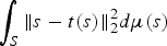 $\int _S \Vert s-t(s) \Vert_2^2 d\mu (s)$ for an appropriate measure μ on S. The forward, backward, and symmetric Hausdorff matching distortions are similarly defined, with the averages replaced by maxima (or integrals replaced by suprema).
Though there can be many variants on these measures, for example using averages in (9)–(10) instead of maxima, or using other norms or robust measures in (5)–(8), these definitions are consistent with those in [Reference Mekuria, Li, Tulvan and Chou43] when  $t^{\ast}(\cdot )$ and $s^{\ast}(\cdot )$ are used as the matching functions. Though we do not use them here, matching functions other than $t^{\ast}(\cdot )$ and $s^{\ast}(\cdot )$, which take color into account and are smoothed, such as in [Reference de Queiroz and Chou41], may yield distortion measures that are better correlated with subjective distortion. In this paper, for consistency with the literature, we use the symmetric mean squared matching distortion with matching functions $t^{\ast}(\cdot )$ and $s^{\ast}(\cdot )$.
For each frame t, we compute the matching distortion between sets  $S^{(t)}$ and $T^{(t)}$, which are obtained by the sampling the texture map of the original HCap data to obtain a high-resolution point cloud $({\bf V}_{rr}^{(t)},\,{\bf C}_{rr}^{(t)})$ with J=10 and U=40. We compare its colors and vertices to the decompressed and color interpolated high resolution point cloud $(\hat {{\bf V}}_{rr}^{(t)},\,\hat {{\bf C}}_{rr}^{(t)})$ with interpolation factor $U_{interp}=4$ described in Section VC.Footnote 2 We then voxelize both point clouds and compute the mean squared matching distortion over all frames as
 $$\bar{d}_G^2 = \displaystyle{1 \over N}\sum\limits_{t = 1}^N {d_G^2 } (S^{(t)},T^{(t)})$$
 $$\bar{d}_Y^2 = \displaystyle{1 \over N}\sum\limits_{t = 1}^N {d_Y^2 } (S^{(t)},T^{(t)})$$
and we report the geometry and color components of the matching distortion in dB as
 $$PSNR_G = -10\log _{10}\displaystyle{{\bar{d}_G^2 } \over {3W^2}}$$
 $$PSNR_Y = -10\log _{10}\displaystyle{{\bar{d}_Y^2 } \over {{255}^2}}$$
where W=1 is the width of the bounding cube.
Note that even though the geometry and color components of the distortion measure are separate, there is an interaction: The geometry affects the matching, and hence affects the color distortion. Thus we will report the color component of the matching distortion as a function of the color stepsize ( $\Delta _{color}$) for a fixed motion stepsize ( $\Delta _{motion}$), and vice versa, to understand the independent effects of geometry and color compression on color quality. We report the geometry component of the matching distortion as a function only of the motion stepsize ( $\Delta _{motion}$), since color compression does not affect the geometry under the assumed matching functions $t^{\ast}(\cdot )$ and $s^{\ast}(\cdot )$.
3) Triangle cloud distortion
In our setting, the input and output of our system are the triangle clouds  $({\bf V}^{(t)},\,{\bf F}^{(t)},\,{\bf C}^{(t)})$ and $(\hat {{\bf V}}^{(t)},\,{\bf F}^{(t)},\,\hat {{\bf C}}^{(t)})$. Thus natural measures of distortion for our system are
 $$PSNR_G = -10\log _{10}\left( {\displaystyle{1 \over N}\sum\limits_{t = 1}^N {\displaystyle{{{\rm \Vert }{\bf V}_r^{(t)} -\widehat{{\bf V}}_r^{(t)} {\rm \Vert }_2^2 } \over {3W^2N_r^{(t)} }}} } \right)$$
 $$PSNR_Y = -10\log _{10}\left( {\displaystyle{1 \over N}\sum\limits_{t = 1}^N {\displaystyle{{{\rm \Vert }{\bf Y}_r^{(t)} -\widehat{{\bf Y}}_r^{(t)} {\rm \Vert }_2^2 } \over {{255}^2N_r^{(t)} }}} } \right),$$
where  ${\bf Y}_r^{(t)}$ is the first (i.e, luminance) column of the $N_r^{(t)}\times 3$ matrix of color attributes ${\bf C}_r^{(t)}$ and W=1 is the width of the bounding cube. These represent the average geometric and luminance distortions across the faces of the triangles. $PSNR_U$ and $PSNR_V$ can be similarly defined.
However, for rendering, we use higher resolution versions of the triangles, in which both the vertices and the colors are interpolated up from  ${\bf V}_r^{(t)}$ and ${\bf C}_r^{(t)}$ using Algorithm 6 to obtain higher resolution vertices and colors ${\bf V}_{rr}^{(t)}$ and ${\bf C}_{rr}^{(t)}$. We use the following distortion measures as very close approximations of (15) and (16):
 $$PSNR_G = -10\log _{10}\left( {\displaystyle{1 \over N}\sum\limits_{t = 1}^N {\displaystyle{{{\rm \Vert }{\bf V}_{rr}^{(t)} -\widehat{{\bf V}}_{rr}^{(t)} {\rm \Vert }_2^2 } \over {3W^2N_{rr}^{(t)} }}} } \right)$$
 $$PSNR_Y = -10\log _{10}\left( {\displaystyle{1 \over N}\sum\limits_{t = 1}^N {\displaystyle{{{\rm \Vert }{\bf Y}_{rr}^{(t)} -\widehat{{\bf Y}}_{rr}^{(t)} {\rm \Vert }_2^2 } \over {{255}^2N_{rr}^{(t)} }}} } \right),$$
where  ${\bf Y}_{rr}^{(t)}$ is the first (i.e, luminance) column of the $N_{rr}^{(t)}\times 3$ matrix of color attributes ${\bf C}_{rr}^{(t)}$ and W=1 is the width of the bounding cube. $PSNR_U$ and $PSNR_V$ can be similarly defined.
4) Transform coding distortion
For the purposes of rate-distortion optimization, and other rapid distortion computations, it is more convenient to use an internal distortion measure: the distortion between the input and output of the transform coder. We call this the transform coding distortion, defined in dB as
 $$PSNR_G = -10\log _{10}\left( {\displaystyle{1 \over N}\sum\limits_{t = 1}^N {\displaystyle{{{\rm \Vert }{\bf V}_v^{(t)} -\widehat{{\bf V}}_v^{(t)} {\rm \Vert }_2^2 } \over {3W^2N_v^{(t)} }}} } \right)$$
 $$PSNR_Y = -10\log _{10}\left( {\displaystyle{1 \over N}\sum\limits_{t = 1}^N {\displaystyle{{{\rm \Vert }{\bf Y}_{rv}^{(t)} -\widehat{{\bf Y}}_{rv}^{(t)} {\rm \Vert }_2^2 } \over {{255}^2N_{rv}^{(t)} }}} } \right),$$
where  ${\bf Y}_{rv}^{(t)}$ is the first (i.e, luminance) column of the $N_{rv}^{(t)}\times 3$ matrix ${\bf C}_{rv}^{(t)}$. $PSNR_U$ and $PSNR_V$ can be similarly defined. Unlike (17)–(18), which are based on system inputs and outputs ${\bf V}^{(t)},\,{\bf C}^{(t)}$ and $\hat {{\bf V}}^{(t)},\,\hat {{\bf C}}^{(t)}$, (19)–(20) are based on the voxelized quantities ${\bf V}_v^{(t)},\,{\bf C}_{rv}^{(t)}$ and $\hat {{\bf V}}_v^{(t)},\,\hat {{\bf C}}_{rv}^{(t)}$, which are defined for reference frames in Algorithm 8 (Steps 3, 6, and 9) and for predicted frames in Algorithm 10 (Steps 2, 7, 9, and 14). The squared errors in the two cases are essentially the same, but are weighted differently: one by face and one by voxel.
C) Rate metrics
As with the distortion, we report bit rates for compression of a whole sequence, for geometry and color. We compute the bit rate averaged over a sequence, in megabits per second, as
 $$R_{Mbps} = \displaystyle{{bits} \over {{1024}^2N}}30\;[{\rm Mbps}]$$
where N is the number of frames in the sequence, and bits is the total number of bits used to encode the color or geometry information of the sequence. Also, we report the bit rate in bits per voxel as
 $$R_{bpv} = \displaystyle{{bits} \over {\sum\limits_{t = 1}^N {N_{rv}^{(t)} } }}\;[{\rm bpv}]$$
where  $N_{rv}^{(t)}$ is the number of occupied voxels in frame t and again bits is the total number of bits used to encode color or geometry for the whole sequence. The number of voxels of a given frame $N_{rv}^{(t)}$ depends on the voxelization used. For example in our triangle cloud encoder, within a GOF all frames have the same number of voxels because the voxelization of attributes is done with respect to the reference frame. For our triangle encoder in all intra-mode, each frame will have a different number of voxels.
D) Intra-frame coding
We first examine the intra-frame coding of triangle clouds, and compare it to intra-frame coding of voxelized point clouds. To obtain the voxelized point clouds, we voxelize the original mesh-based sequences Man, Soccer, and Breakers by refining each face in the original sequence by upsampling factor U=10, and voxelizing to level J=10. For each sequence, and each frame t, this produces a list of occupied voxels  ${\bf V}_{rv}^{(t)}$ and their colors ${\bf C}_{rv}$.
1) Intra-frame coding of geometry
We compare our method for coding geometry in reference frames with the previous state-of-the-art for coding geometry in single frames. The previous state-of-the art for coding the geometry of voxelized point clouds [Reference Meagher24,Reference Schnabel and Klein29,Reference Kammerl, Blodow, Rusu, Gedikli, Beetz and Steinbach31,Reference Ochotta and Saupe46] codes the set of occupied voxels  ${\bf V}_{rv}^{(t)}$ by entropy coding the octree description of the set. In contrast, our method first approximates the set of occupied voxels by a set of triangles, and then codes the triangles as a triple $({\bf V}_v^{(t)},\,{\bf F}^{(t)},\,{\bf I}_v^{(t)})$. The vertices ${\bf V}_v^{(t)}$ are coded using octrees plus gzip, the faces ${\bf F}^{(t)}$ are coded directly with gzip, and the indices ${\bf I}_v^{(t)}$ are coded using run-length encoding plus gzip as described in Section 1. When the geometry is smooth, relatively few triangles need to be used to approximate it. In such cases, our method gains because the list of vertices ${\bf V}_v^{(t)}$ is much shorter than the list of occupied voxels ${\bf V}_{rv}^{(t)}$, even though the list of triangle indices ${\bf F}^{(t)}$ and the list of repeated indices ${\bf I}_v^{(t)}$ must also be coded.
Taking all bits into account, Table 3 shows the bit rates for both methods in megabits per second (Mbps) and bits per occupied voxel (bpv) averaged over the sequences. Our method reduces the bit rate needed for intra-frame coding of geometry by a factor of 5–10, breaking through the 2.5 bpv rule-of-thumb for octree coding.
Intra-frame coding of the geometry of voxelized point clouds. “Previous” refers to our implementation of the octree coding approach described in [Reference Meagher24,Reference Schnabel and Klein29,Reference Kammerl, Blodow, Rusu, Gedikli, Beetz and Steinbach31,Reference Ochotta and Saupe46]

While it is true that approximating the geometry by triangles is generally not lossless, in this case, the process is lossless because our ground truth datasets are already described in terms of triangles.
2) Intra-frame coding of color
Our method of coding color in reference frames is identical with the state-of-the art for coding color in single frames, using transform coding based on RAHT, described in [Reference de Queiroz and Chou34]. For reference, the rate-distortion results for color intra-frame coding are shown in Fig. 12 (where we compare to color inter-frame coding).
E) Temporal coding: transform coding distortion-rate curves
We next examine temporal coding, by which we mean intra-frame coding of the first frame, and inter-frame coding of the remaining frames, in each GOF as defined by stretches of consistent connectivity in the datasets. We compare temporal coding to all-intra coding of triangle clouds using the transform coding distortion. We show that temporal coding provides substantial gains for geometry across all sequences, and significant gains for color on one of the three sequences.
1) Temporal coding of geometry
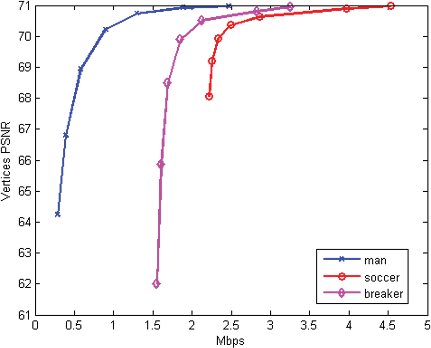
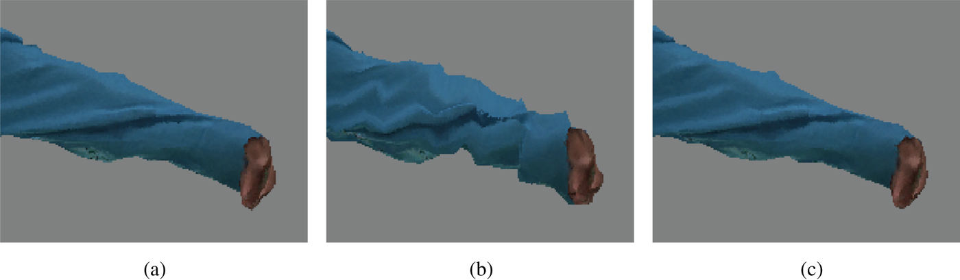
Figure 7 shows the geometry transform coding distortion  $PSNR_G$ (19) as a function of the bit rate needed for geometry information in the temporal coding of the sequences Man, Soccer, and Breakers. It can be seen that the geometry PSNR saturates, at relatively low bit rates, at the highest fidelity possible for a given voxel size $2^{-J}$, which is 71 dB for J=10. In Fig. 8, we show on the Breakers sequence that quality within $0.5\,dB$ of this limit appears to be sufficiently close to that of the original voxelization without quantization. At this quality, for Man, Soccer, and Breakers sequences, the encoder in temporal coding mode has geometry bit rates of about 1.2, 2.7, and 2.2 Mbps (corresponding to 0.07, 0.19, 0.17 bpv [Reference Pavez, Chou, de Queiroz and Ortega47]), respectively. For comparison, the encoder in all-intra coding mode has geometry bit rates of 5.24, 6.39, and 4.88 Mbps (0.33, 0.44, 0.36 bpv), respectively, as shown in Table 3. Thus temporal coding has a geometry bit rate savings of a factor of 2–5 over our intra-frame coding only, and a factor of 13–45 over previous intra-frame octree coding.
RD curves for temporal geometry compression. Rates include all geometry information.
Visual quality of geometry compression. Bit rates correspond to all geometry information. (a) original, (b) 62 dB (1.6 Mbps), (c) 70.5 dB (2.2 Mbps).
A temporal analysis is provided in Figs 9 and 10. Figure 9 shows the number of kilobits per frame needed to encode the geometry information for each frame. The number of bits for the reference frames are dominated by their octree descriptions, while the number of bits for the predicted frames depends on the quantization stepsize for motion residuals,  $\Delta _{motion}$. We observe that a significant bit reduction can be achieved by lossy coding of residuals. For $\Delta _{motion}=4$, there is more than a 3x reduction in bit rate for inter-frame coding relative to intra-frame coding.
Kilobits/frame required to code the geometry information for each frame for different values of the motion residual quantization stepsize  $\Delta _{motion} \in \lbrace 1,\,2,\,4,\,8\rbrace $. Reference frames encode ${\bf V}^{(1)}_v$ using octree coding plus gzip and encode ${\bf I}_v^{(1)}$ using run-length coding plus gzip. Predicted frames encode their motion residuals $\Delta {\bf V}^{(t)}$ using transform coding. (a) Man, (b) Soccer, (c) Breakers.

Mean squared quantization error required to code the geometry information for each frame for different values of the motion residual quantization stepsize  $\Delta _{motion} \in \lbrace 1,\,2,\,4,\,8\rbrace $. Reference frames encode ${\bf V}^{(1)}_v$ using octrees; hence the distortion is due to quantization error is $\epsilon ^2$. Predicted frames encode their motion residuals $\Delta {\bf V}^{(t)}$ using transform coding. (a) Man, (b) Soccer, (c) Breaker.

Figure 10 shows the mean squared quantization error
 $$MSE_G = \displaystyle{1 \over N}\sum\limits_{t = 1}^N {\displaystyle{{{\rm \Vert }{\bf V}_v^{(t)} -\widehat{{\bf V}}_v^{(t)} {\rm \Vert }_2^2 } \over {3W^2N_v^{(t)} }}},$$
which corresponds to the  $PSNR_G$ in (19). Note that for reference frames, the mean squared error is well approximated by
 $$\displaystyle{{{\rm \Vert }{\bf V}_v^{(1)} -\widehat{{\bf V}}_v^{(1)} {\rm \Vert }_2^2 } \over {3W^2N_v^{(t)} }}\approx \displaystyle{{2^{-2J}} \over {12}}\mathop = \limits^\Delta {\rm \epsilon }^2.$$
Thus for reference frames, the  $MSE_G$ falls to $\epsilon ^2$, while for predicted frames, the $MSE_G$ rises from $\epsilon ^2$ depending on the motion stepsize $\Delta _{motion}$.
2) Temporal coding of color
To evaluate color coding, first, we consider separate quantization stepsizes for reference and predicted frames  $\Delta _{color,intra}$ and $\Delta _{color,inter}$, respectively. Both take values in $\{1,\, 2,\, 4,\, 8,\, 16,\, 32,\, 64\}$.
Figure 11 shows the color transform coding distortion  $PSNR_Y$ (20) as a function of the bit rate needed for all (Y , U, V ) color information for temporal coding of the sequences Man, Soccer, and Breakers, for different combinations of $\Delta _{color,intra}$ and $\Delta _{color,inter}$, where each colored curve corresponds to a fixed value of $\Delta _{color,intra}$. It can be seen that the optimal RD curve is obtained by choosing $\Delta _{color,intra}=\Delta _{color,inter}$, as shown in the dashed line.
Luminance (Y) component rate-distortion performances of (top) Man, (middle) Soccer and (bottom) Breakers sequences, for different intra-frame stepsizes  $\Delta _{color,intra}$. Rate includes all (Y , U, V ) color information.

Temporal coding versus all-intra coding. The bit rate contains all (Y , U, V ) color information, although the distortion is only the luminance (Y ) PSNR.
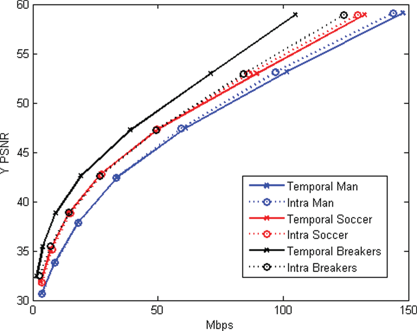
Next, we consider equal quantization stepsizes for reference and predicted frames, hereafter designated simply  $\Delta _{color}$.
Figure 12 shows the color transform coding distortion  $PSNR_Y$ (20) as a function of the bit rate needed for all (Y , U, V ) color information for temporal coding and all-intra coding on the sequences Man, Soccer, and Breakers. We observe that temporal coding outperforms all-intra coding by 2-3 dB for the Breakers sequence. However, for the Man and Soccer sequences, their RD performances are similar. Further investigation is needed on when and how gains can be achieved by the predictive coding of color.
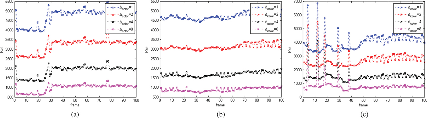
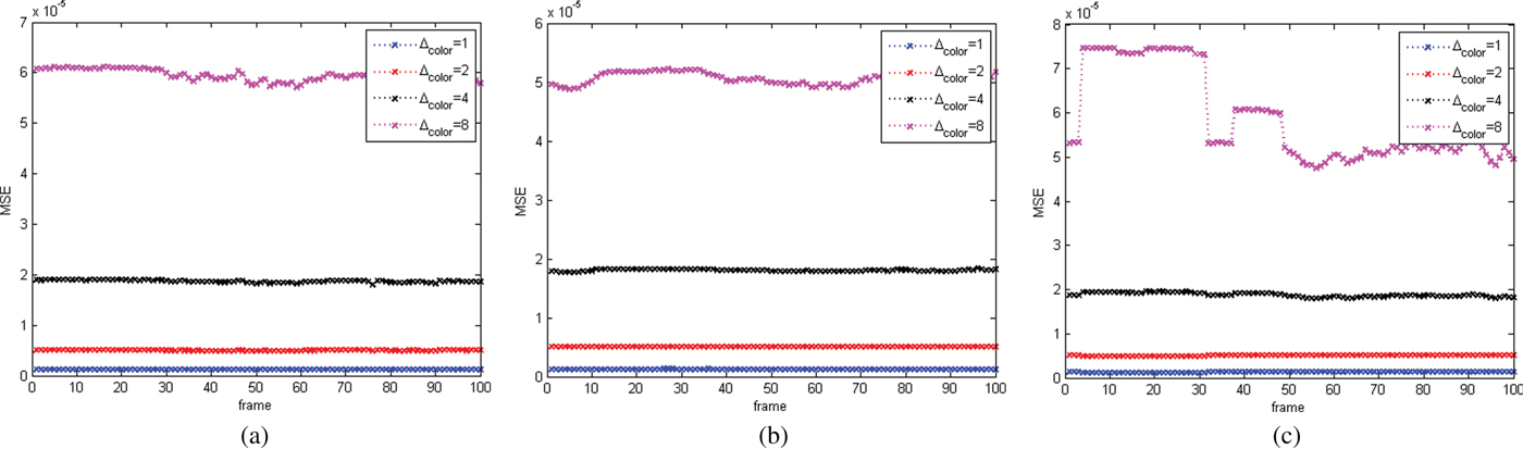
A temporal analysis is provided in Figs 13 and 14. In Fig. 13, we show the bit rates (Kbit) to compress the color information for the first 100 frames of all sequences. We observe that, as expected, for smaller values of  $\Delta _{color}$ the bit rates are higher, for all frames. For Man and Soccer sequences, we observe that the bit rates do not vary much from reference frames to predicted frames; however, in the Breakers sequence, it is clear that for all values of $\Delta _{color}$ the reference frames have much higher bit rates compared to predicted frames, which confirms the results from Fig. 12, where temporal coding provides gains with respect to all-intra coding of triangle clouds for the Breakers sequence, but not for the Man and Soccer sequences. In Fig. 14, we show the mean squared error (MSE) of the Y color component for the first 100 frames of all sequences. For $\Delta _{color} \leq 4$ the error is uniform across all frames and sequences.
Kilobits/frame required to code the color information for each frame for different values of the color residual quantization stepsize  $\Delta _{color} \in \lbrace 1,\,2,\,4,\,8\rbrace $. Reference frames encode their colors ${\bf C}_{rv}^{(1)}$ and predicted frames encode their color residuals $\Delta {\bf C}_{rv}^{(t)}$ using transform coding. (a) Man, (b) Soccer, (c) Breakers.
Mean squared quantization error required to code the color information for each frame for different values of the color residual quantization stepsize  $\Delta _{color} \in \lbrace 1,\,2,\,4,\,8\rbrace $. Reference frames encode their colors ${\bf C}_{rv}^{(1)}$ and predicted frames encode their color residuals $\Delta {\bf C}_{rv}^{(t)}$ using transform coding. (a) Man, (b) Soccer, (c) Breakers.
3) Comparison of dynamic mesh compression
We now compare our results to the dynamic mesh compression in [Reference Anis, Chou and Ortega21], which uses a distortion measure similar to the transform coding distortion measure, and reports results on a version of the Man sequence.
For geometry coding, Fig. 5 in [Reference Anis, Chou and Ortega21] shows that when their geometry distortion is 70.5 dB, their geometry bit rate is about 0.45 bpv. As shown in Fig. 7, at the same distortion, our bit rate is about 1.2 Mbps (corresponding to about 0.07 bpv [Reference Pavez, Chou, de Queiroz and Ortega47]), which is lower than their bit rate by a factor of 6x or more.
For color coding, Fig. 5 in [Reference Anis, Chou and Ortega21] shows that when their color distortion is 40 dB, their color bit rate is about 0.8 bpv. As shown in Fig. 12, at the same distortion, our bit rate is about 30 Mbps (corresponding to about 1.8 bpv [Reference Pavez, Chou, de Queiroz and Ortega47]).
Overall, their bit rate would be about 0.45+0.8=1.3 bpv, while our bit rate would be about 0.07+1.8=1.9 bpv. However, it should be cautioned that the sequence compressed in [Reference Anis, Chou and Ortega21] is not the original Man sequence used in our work but rather a smooth mesh fit to a low-resolution voxelization (J=9) of the sequence. Hence it has smoother color as well as smoother geometry, and should be easier to code. Nevertheless, it is a point of comparison.
F) Temporal coding: triangle cloud, projection, and matching distortion-rate curves
In this section, we show distortion rate curves using the triangle cloud, projection, and matching distortion measures. All distortions in this section are computed from high-resolution triangle clouds generated from the original HCap data, and from the decompressed triangle clouds. For computational complexity reasons, we show results only for the Man sequence, and consider only its first four GOFs (120 frames).
1) Geometry coding
First, we analyze the triangle cloud distortion and matching distortion of geometry as a function of geometry bit rate. The RD plots are shown in Fig. 15. We observe that both distortion measures start saturating at the same point as for the transform coding distortion: around  $\Delta _{motion}=4$. However, for these distortion measures, the saturation is not as pronounced. This suggests that these distortion measures are quite sensitive to small amounts of geometric distortion.
RD curves for geometry triangle cloud and matching distortion versus geometry bit rates (Man sequence).
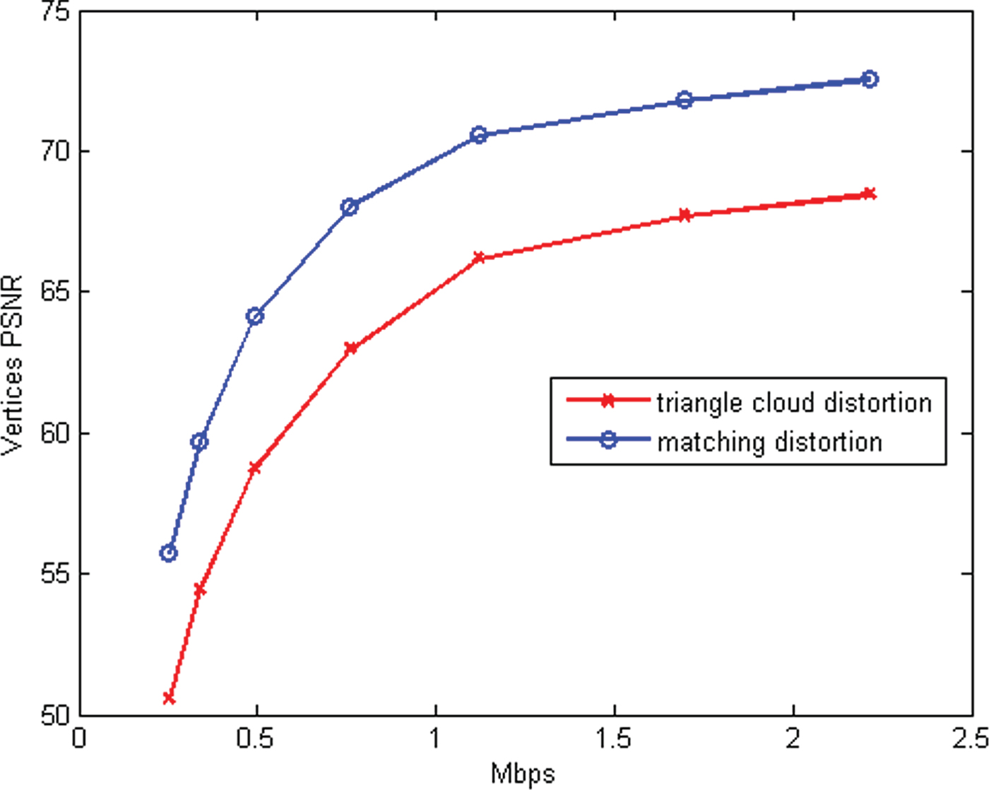
Next, we study the effect of geometry compression on color quality. In Fig. 16, we show the Y component PSNR for the projection and matching distortion measures. The color has been compressed at the highest bit rate considered, using the same quantization step for intra and inter color coding,  $\Delta _{color}=1$. Surprisingly, we observe a significant influence of the geometry compression on these color distortion measures, particular for $\Delta _{motion}>4$. This indicates very high sensitivity to geometric distortion of the projection distortion measure and the color component of the matching distortion measure. This hyper-sensitivity can be explained as follows. For the projection distortion measure, geometric distortion causes local shifts of the image. As is well known, PSNR, as well as other image distortion measures including structural similarity index, fall apart upon image shifts. For the matching metric, since the matching functions $s^{\ast}$ and $t^{\ast}$ depend only on geometry, geometric distortion causes inappropriate matches, which affect the color distortion across those matches.
RD curves for color triangle cloud and matching distortion versus geometry bit rates (Man sequence). The color stepsize is set to  $\Delta _{color}=1$.
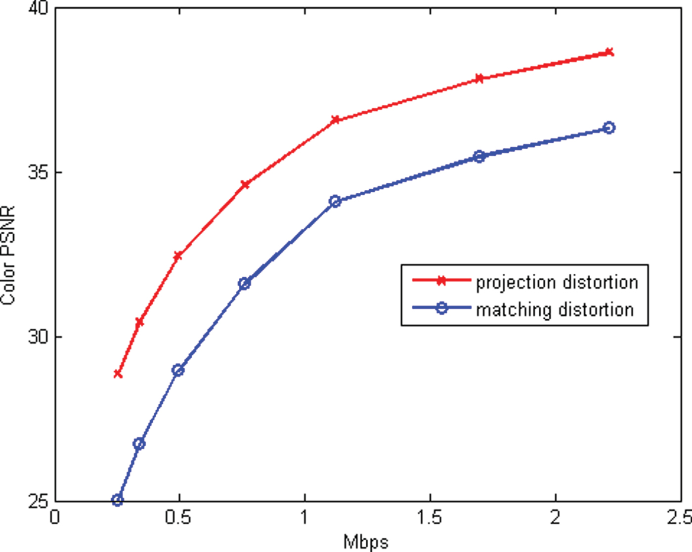
2) Color coding
Finally, we analyze the RD curve for color coding as a function of color bit rate. We plot Y component PSNR for the triangle cloud, projection, and matching distortion measures in Fig. 17. For this experiment, we consider the color quantization steps equal for intra and inter coded frames. The motion step is set to  $\Delta _{motion}=1$. For all three distortion measures, the PSNR saturates very quickly. Apparently, this is because the geometry quality severely limits the color quality under any of these three distortion measures, even when the geometry quality is high ( $\Delta _{motion}=1$). In particular, when $\Delta _{motion}=1$, for color quantization stepsizes smaller than $\Delta _{color}=8$, color quality does not improve significantly under these distortion measures, while under the transform coding distortion measure, the PSNR continues to improve, as shown in Fig. 11. Whether the hyper-sensitivity of the color projection and color matching distortion measures to geometric distortion are perceptually justified is questionable, but open to further investigation.
RD curves for color triangle cloud, projection, and matching distortion versus color bit rates (Man sequence). The motion stepsize is set to  $\Delta _{motion}=1$.
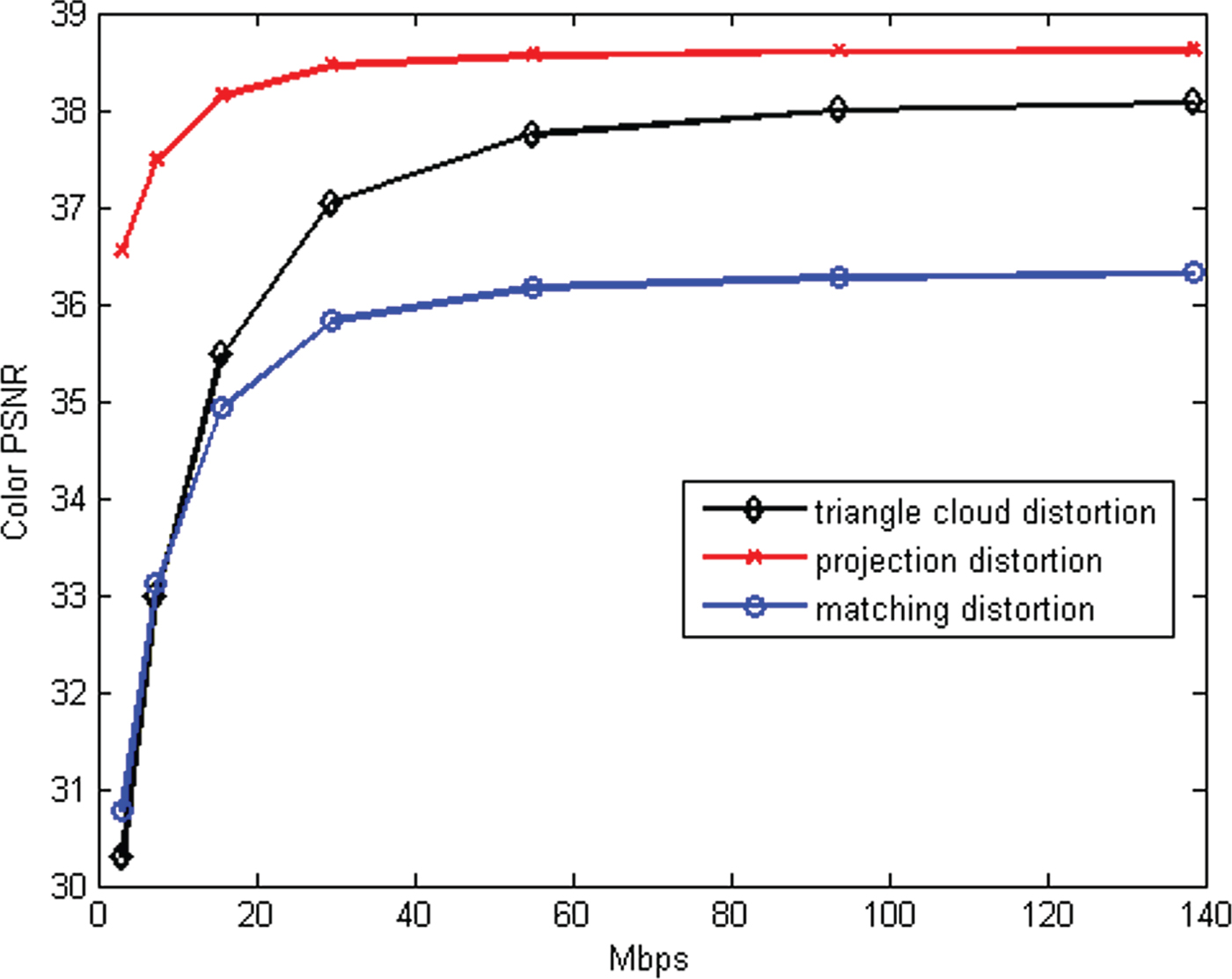
3) Comparison of dynamic point cloud compression
Notwithstanding possible issues with the color projection distortion measure, it provides an opportunity to compare our results on dynamic triangle cloud compression to the results on dynamic point cloud compression in [Reference de Queiroz and Chou41]. Like us, [Reference de Queiroz and Chou41] reports results on a version of the Man sequence, using the projection distortion measure.
Figure 17 shows that for triangle cloud compression, the projection distortion reaches 38.5 dB at around 30 Mbps (corresponding to less than 2 bpv [Reference Pavez, Chou, de Queiroz and Ortega47]). In comparison, Fig. 10a in [Reference de Queiroz and Chou41] shows that for dynamic point cloud compression, the projection distortion reaches 38.5 dB at around 3 bpv. Hence it seems that our dynamic triangle cloud compression may be more efficient than point cloud compression under the projection distortion measure. However, it should be cautioned that the sequence compressed in [Reference de Queiroz and Chou41] is a lower resolution (J=9) version of the Man sequence rather than the higher resolution version (J=10) used in our work. Moreover, Fig. 17 in our paper reports the distortion between the original signal (with uncoded color and uncoded geometry) to the coded signal (with coded color and coded geometry), while Fig. 10a in [Reference de Queiroz and Chou41] reports the distortion between the signal with uncoded color and coded geometry to the signal with coded color and identically coded geometry. In the latter case, the saturation of the color measure due to geometric coding is not apparent.
VII. CONCLUSION
When coding for video, the representation of the input to the encoder and the representation of the output of the decoder are clear: sequences of rectangular arrays of pixels. Furthermore, distortion measures between the two representations are well accepted in practice.
Two leading candidates for the codec's representation for augmented reality to this point have been dynamic meshes and dynamic point clouds. Each has its advantages and disadvantages. Dynamic meshes are more compressible but less robust to noise and non-surface topologies. Dynamic point clouds are more robust, but removing spatio-temporal redundancies is much more challenging, making them difficult to compress.
In this paper, we proposed dynamic polygon clouds, which have the advantages of both meshes and point clouds, without their disadvantages. We provided detailed algorithms on how to compress them, and we used a variety of distortion measures to evaluate their performance.
For intra-frame coding of geometry, we showed that compared to the previous state-of-the-art for intra-frame coding of the geometry of voxelized point clouds, our method reduces the bit rate by a factor of 5–10 with negligible (but non-zero) distortion, breaking through the 2.5 bpv rule-of-thumb for lossless coding of geometry in voxelized point clouds. Intuitively, these gains are achieved by reducing the representation from a dense list of points to a less dense list of vertices and faces.
For inter-frame coding of geometry, we showed that compared to our method of intra-frame coding of geometry, we can reduce the bit rate by a factor of 3 or more. For temporal coding, this results in a geometry bit rate savings of a factor of 2–5 over all-intra coding. Intuitively, these gains are achieved by coding the motion prediction residuals. Multiplied by the 5–10 x improvement of our intra-frame coding compared to previous octree-based intra-frame coding, we have demonstrated a 13–45 x reduction in bit rate over previous octree-based intra-frame coding.
For inter-frame coding of color, we showed that compared to our method of intra-frame coding of color (which is the same as the current state-of-the-art for intra-frame coding of color [Reference de Queiroz and Chou34]), our method reduces the bit rate by about 30% or alternatively increases the PSNR by about 2 dB (at the relevant level of quality) for one of our three sequences. For the other two sequences, we found little improvement in performance relative to the intra-frame coding of color. This is a matter for further investigation, but one hypothesis is that the gain is dependent upon the quality of the motion estimation. Intuitively, gains are achieved by coding the color prediction residuals, and the color prediction is accurate only if the motion estimation is accurate.
We compared our results on triangle cloud compression to recent results in dynamic mesh compression and dyanamic point cloud compression. The comparisons are imperfect due to somewhat different datasets and distortion measures, which likely favor the earlier work. However, they indicate that compared to dynamic mesh compression, our geometry coding may have a bit rate 6x lower, while our color coding may have a bit rate 2.25x higher. At the same time, compared to dynamic point cloud compression, our overall bit rate may be about 33% lower.
Our work also revealed the hyper-sensitivity of distortion measures such as the color projection and color matching distortion measures to geometry coding.
Future work includes better transforms and better entropy coders, RD optimization, better motion compensation, more perceptually relevant distortion measures and post-processing filtering.
ACKNOWLEDGMENTS
The authors would like to thank the Microsoft HoloLens Capture (HCap) team for making their data available to this research, and would also like to thank the Microsoft Research Interactive 3D (I3D) team for many discussions.
FINANCIAL SUPPORT
None.
STATEMENT OF INTEREST
None.
APPENDIX
Refinement (refine)

Refinement and Color Interpolation

Uniform scalar quantization (quantize)

Encode reference frame (I-encoder)

Decode reference frame (I-decoder)

Encode predicted frame (P-encoder)

Decode predicted frame (P-decoder)

Eduardo Pavez received his B.S. and M.Sc. degrees in Electrical Engineering from Universidad de Chile, Santiago, Chile, in 2011 and 2013, respectively.
He is currently a Ph.D. student in Electrical Engineering at the University of Southern California (USC), Los Angeles, USA. His research interests include graph signal processing, graph estimation, and multimedia compression.
Philip A. Chou received the B.S.E degree in electrical engineering and computer science from Princeton University, Princeton, NJ, and the M.S. degree in electrical engineering and computer science from the University of California, Berkeley, in 1980 and 1983, respectively, and the Ph.D. degree in electrical engineering from Stanford University in 1988. From 1988 to 1990, he was a member of Technical Staff at AT & T Bell Laboratories, Murray Hill, NJ. From 1990 to 1996, he was a member of Research Staff, Xerox Palo Alto Research Center, Palo Alto, CA. In 1997, he was a Manager of the Compression Group, VXtreme, Mountain View, CA, an Internet video startup before it was acquired by Microsoft. From 1998 to 2016, he was a Principal Researcher with Microsoft Research, Redmond, Washington, where he was managing the Communication and Collaboration Systems Research Group from 2004 to 2011. He served as Consulting Associate Professor at Stanford University from 1994 to 1995, Affiliate Associate Professor with the University of Washington from 1998 to 2009, and an Adjunct Professor with the Chinese University of Hong Kong since 2006. He was with a startup, 8i.com, where he led the effort to compress and communicate volumetric media, popularly known as holograms, for virtual and augmented reality. In September 2018, he joined the Google Daydream group as a Research Scientist.
Ricardo L. de Queiroz received the Engineer degree from Universidade de Brasilia, Brazil, in 1987, the M.Sc. degree from Universidade Estadual de Campinas, Brazil, in 1990, and the Ph.D. degree from The University of Texas at Arlington, in 1994, all in Electrical Engineering. In 1990-1991, he was with the DSP research group at Universidade de Brasilia, as a research associate. He joined Xerox Corp. in 1994, where he was a member of the research staff until 2002. In 2000–2001 he was also an Adjunct Faculty at the Rochester Institute of Technology. He joined the Electrical Engineering Department at Universidade de Brasilia in 2003. In 2010, he became a Full (Titular) Professor at the Computer Science Department at Universidade de Brasilia. During 2015 he has been a Visiting Professor at the University of Washington, in Seattle. Dr. de Queiroz has published extensively in Journals and conferences and contributed chapters to books as well. He also holds 46 issued patents. He is a past elected member of the IEEE Signal Processing Society's Multimedia Signal Processing (MMSP) and the Image, Video and Multidimensional Signal Processing (IVMSP) Technical Committees. He is an editor for IEEE Transactions on Image Processing and a past editor for the EURASIP Journal on Image and Video Processing, IEEE Signal Processing Letters, and IEEE Transactions on Circuits and Systems for Video Technology. He has been appointed an IEEE Signal Processing Society Distinguished Lecturer for the 2011–2012 term. Dr. de Queiroz has been actively involved with IEEE Signal Processing Society chapters in Brazil and in the USA. He was the General Chair of ISCAS'2011, MMSP'2009, and SBrT'2012. He was also part of the organizing committee of many SPS flagship conferences. His research interests include image and video compression, point cloud compression, multirate signal processing, and color imaging. Dr. de Queiroz is a Fellow of IEEE and a member of the Brazilian Telecommunications Society.
Antonio Ortega received the Telecommunications Engineering degree from the Universidad Politecnica de Madrid, Madrid, Spain in 1989 and the Ph.D. in Electrical Engineering from Columbia University, New York, NY in 1994. In 1994, he joined the Electrical Engineering department at the University of Southern California (USC), where he is currently a Professor and has served as Associate Chair. He is a Fellow of IEEE and EURASIP, and a member of ACM and APSIPA. He is currently a member of the Board of Governors of the IEEE Signal Processing Society. He was the inaugural Editor-in-Chief of the APSIPA Transactions on Signal and Information Processing. He has received several paper awards, including most recently the 2016 Signal Processing Magazine award and was a plenary speaker at ICIP 2013. His recent research work is focusing on graph signal processing, machine learning, multimedia compression and wireless sensor networks. Over 40 Ph.D. students have completed their Ph.D. thesis under his supervision at USC and his work has led to over 300 publications, as well as several patents.

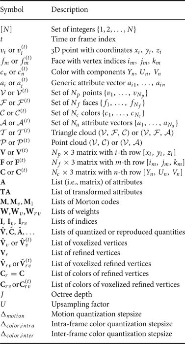


 Open access

