


Policy Significance Statement
This research shows how the latest advances in data science, which focus on identifying causal pathways and assessing the relative likelihood of those causal pathways, can be useful in policymaking across a range of policy domains. By representing the set of complex factors that impact an outcome as an easy-to-interpret network of stratified factors, policymakers can judge how a policy intervention will impact not only a single outcome but the entire network of factors. This will provide policymakers with a more comprehensive understanding of complex issues at play and enable the identification of optimal policies for specific social challenges.
1. Introduction
The policymaking landscape is inherently complex, particularly in high-stakes situations such as education, healthcare, and environmental policy, where decisions have profound and far-reaching consequences (Mueller, Reference Mueller2020). These high-stakes situations are characterised by multifaceted, interrelated factors and ambiguous futures. Accounting for complexity and the associated uncertainty is key to good policy setting and decision-making in such situations, (Cripps and Durrant-Whyte, Reference Cripps and Durrant-Whyte2023).
An example of this complexity can be seen in education, where policymakers face the challenge of improving student attendance and learning outcomes, especially in disadvantaged communities. This issue is influenced by complex, interrelated factors such as socio-economic status and access to healthcare. These factors are often difficult to disentangle using traditional data science techniques.
Traditional techniques like linear regression reduce complex policy issues to a single outcome and a limited set of inputs, often resulting in oversimplified models that overlook key interrelationships between variables. These models assume linearity and independence among variables, limiting their ability to capture the intricate dynamics of real-world policy challenges. In contrast, more advanced methods, such as random forests and neural networks, better handle complexity and nonlinear relationships. However, random forests, while robust, lack the interpretability needed in policy contexts, and neural networks, though powerful, function as “black boxes” with limited transparency. Despite their ability to model complexity, these methods often fail to deliver the causal insights and clarity essential for effective decision-making in policy.
Recent advancements in causal machine learning have provided valuable new tools for policymaking, particularly through the use of probabilistic graphical models like Bayesian networks, which offer a more nuanced understanding of complex causal relationships (Scholköpf, Reference Schölkopf2022; Lechner, Reference Lechner2023; Kaddour et al., Reference Kaddour, Lynch, Liu, Kusner and Silva2022; Moreira Reference Moreira, Chou, Velmurugan, Ouyang, Sindhgatta and Bruza2021). A Bayesian network (BN) is a graphical model that is commonly used to represent causal pathways (Schölkopf, Reference Schölkopf2022; Kaddour et al., Reference Kaddour, Lynch, Liu, Kusner and Silva2022). A BN shows the dependencies that exist between factors, whereby factors, we mean variables or features of an environment that may impact outcomes. A BN consists of nodes representing factors and directed edges, indicating dependencies between factors. Arrows are attached to edges, and the factor from which an arrow originates is called a parent of the factor to which the arrow points, known as a child. This notion of a parent leading to a child gives BNs a causal interpretation. To allow this causal interpretation, a BN is constructed so that the flow of arrows does not permit a cycle (which would imply a self-causality is challenging to interpret), and a BN is therefore also known as a Directed Acyclical Graph (DAG) (Friedman and Koller, Reference Friedman and Koller2003).
One use of DAGs in policy setting, and many other applications, is that the ancestors of a child can be separated into those which are directly linked and are therefore immediate causes, referred to as parents and those ancestors that are indirectly linked, via an intermediate factor, often referred to as root or upstream causes (Zhu et al., Reference Zhu, Marchant, Morris, Baur, Simpson and Cripps2023). This distinction between immediate and upstream causes has implications for policy setting. An intervention on an immediate cause may not have the desired impact on an outcome if upstream or root causes are not addressed. We illustrate this with a simulated example in Section 3, as well as with a real application in Section 4. An active area of research in machine learning, commonly known as causal discovery (Glymour et al., Reference Glymour, Zhang and Spirtes2019), involves learning the structure of a DAG. This process of causal discovery consists of identifying which edges exist and the direction of arrows connecting those edges, which may suggest a causal relationship.
Several methods have been proposed to learn the structure of a DAG using observational data. These methods are mostly divided into constraint-based and scoring approaches. Constraint approaches focus on statistical tests to determine causal dependencies between factors (for example, PC-algorithm (Spirtes et al., Reference Spirtes, Glymour and Scheines2000)). On the other hand, scoring approaches focus on maximising scoring metrics (for instance, the K2 algorithm (Cooper and Herskovits, Reference Cooper and Herskovits1992) and greedy hill climbing (Tsamardinos et al., Reference Tsamardinos, Brown and Aliferis2006)). The recent works of Vowels et al. (Reference Vowels, Camgoz and Bowden2022) and Kitson et al. (Reference Kitson, Constantinou, Guo, Liu and Chobtham2023) provide a comprehensive survey of causal discovery methods and their applications.
Understanding these causal relationships is crucial for accurately quantifying the outcomes of interventions, such as policy changes (Cordero et al., Reference Cordero, Cristóbal and Santín2018) or medical treatments (Matthay and Glymour, Reference Matthay and Glymour2022). This has wide-ranging implications across various fields, from improving public health strategies (Chiolero, Reference Chiolero2018; Zhu et al., Reference Zhu, Marchant, Morris, Baur, Simpson and Cripps2023) to optimising business processes (Bozorgi et al., Reference Bozorgi, Dumas, Rosa, Polyvyanyy, Shoush and Teinemaa2023) and shaping effective government policies (Brock et al., Reference Brock, Durlauf and West2007).
More recent advances in structure learning take a Bayesian approach and focus on attaching relative probabilities to multiple possible causal pathways, in contrast to the previously mentioned constraint-based and score-based approaches that focus on learning a DAG with the single most likely causal pathway. Bayesian structure learning attempts to learn the relative probabilities of all possible causal pathways and typically uses Markov Chain Monte Carlo (MCMC) methods such as structure MCMC (Madigan et al., Reference Madigan, York and Allard1995), order MCMC (Friedman and Koller, Reference Friedman and Koller2003) or partition MCMC (PMCMC) (Kuipers and Moffa, Reference Kuipers and Moffa2017), to obtain sampling-based estimates of these relative probabilities. These techniques, which consider a suite of possible causal pathways over those that focus on a single most likely causal pathway, are of particular relevance in policy settings, where the complexity of the issue inevitably results in the probability of multiple possible causal pathways.
A further advantage of Bayesian structure learning is that prior knowledge from experts or communities can be incorporated into the process (Hassall et al., Reference Hassall, Dailey, Zawadzka, Milne, Harris, Corstanje and Whitmore2019). In ecology, for example, Carriger et al. (Reference Carriger, Barron and Newman2016) suggests that the use of Bayesian structure learning improves evidence-based assessments in areas such as environmental policy by integrating prior knowledge with new evidence. The intersection of policymaking and advanced machine-learning methods has also been a focus of increasing interest in the academic community. For instance, Carriger et al. (Reference Carriger, Barron and Newman2016) emphasises the importance of a DAG in significantly improving environmental assessments for evidence-based policy by merging probabilistic calculus with causal knowledge (Pearl et al., Reference Pearl2000; Pearl and Mackenzie, Reference Pearl and Mackenzie2018).
The integration of Bayesian causal discovery methodologies together with Bayesian reasoning, specifically Bayesian adaptive learning (Cripps et al., Reference Cripps, Lopatnikova, Afshar, Gales, Marchant, Francis, Moreira and Fischer2024), into the policymaking cycle provides a coherent and logically consistent approach for policymakers wishing to make evidenced-based decisions and learn what policies work and why in an adaptive and agile fashion. Bayesian causal discovery provides a useful tool for policymakers seeking to untangle which factors impact outcomes and distinguish proximal or immediate causes from upstream and root causes to identify potential inventions. When coupled with Bayesian reasoning, the impact of an intervention, suggested by the Bayesian causal discovery, can be evaluated so that a continuous and iterative learning cycle is created (Cripps et al., Reference Cripps, Lopatnikova, Afshar, Gales, Marchant, Francis, Moreira and Fischer2024). This topic is the subject of current research in the machine-learning community (Toth et al., Reference Toth, Lorch, Knoll, Krause, Pernkopf, Peharz and von Kügelgen2022).
This paper demonstrates how Bayesian Structure learning can be used to inform policy decision-making in three specific ways.
-
1. We show how DAGs can used to quantify and represent causal pathways, in a statistically rigorous yet readily interpretable manner, making them a useful tool for policymakers to represent how factors affect outcomes in complex social phenomena. These representations stratify factors into those directly connected to an outcome and those indirectly connected to an outcome via intermediate factors. This stratification is suggestive of causal pathways, thereby providing policymakers with an understanding of how multiple factors affect multiple outcomes for targeted policy settings. We give a simple synthetic example of this representation in Section 3.
-
2. We show that estimating a DAG in a Bayesian framework allows us to attach probabilities to many possible causal pathways rather than only estimating the single most likely pathway. This is critical for policymaking in complex environments because it is likely that there are several probable causal pathways. We show, in Sections 2 and 4, that the uncertainty surrounding causal pathways needs to be taken into consideration by policymakers because near equally probable causal pathways are often different and hence would suggest different potential interventions.
-
3. We demonstrate the technique on a real application, where the goal is to find the possible casual pathways for school attendance, which occur beyond the school gate. We use the data from the Longitudinal Study of Australian Children (LSAC) (Mohal et al., Reference Mohal, Lansangan, Gasser, Taylor, Renda, Jessup and Daraganova2021) and show how financial stability affects health-related factors which ultimately drive school attendance.
2. Bayesian networks
Bayesian networks (BNs) are a useful tool for modelling complex relationships between factors. A BN, or DAG consists of a graph, $ \mathcal{G} $
, and conditional on
$ \mathcal{G} $
, and conditional on $ \mathcal{G} $
, a set of parameters,
$ \mathcal{G} $
, a set of parameters, $ \Theta $
. The graph
$ \Theta $
. The graph $ \mathcal{G} $
is defined by a set of nodes or vertices,
$ \mathcal{G} $
is defined by a set of nodes or vertices, $ \mathcal{V} $
and directed edges
$ \mathcal{V} $
and directed edges $ \mathrm{\mathcal{E}} $
, so that
$ \mathrm{\mathcal{E}} $
, so that $ \mathcal{G}=\left\{\mathcal{V},\mathrm{\mathcal{E}}\right\} $
. The parameters
$ \mathcal{G}=\left\{\mathcal{V},\mathrm{\mathcal{E}}\right\} $
. The parameters $ \Theta $
describe the conditional distributions of the nodes,
$ \Theta $
describe the conditional distributions of the nodes, $ \mathcal{V} $
in the graph, where the conditioning is w.r.t the parents of that node; see Appendix B for further details.
$ \mathcal{V} $
in the graph, where the conditioning is w.r.t the parents of that node; see Appendix B for further details.
Structure learning involves determining the optimal arrangement of nodes and edges in a BN from data. Learning the structure of a graph from data is difficult for two main reasons. First, the number of possible graph structures increases super exponentially with the number of nodes, making an exhaustive search over all possible graphs computationally infeasible, even for a modest number of nodesFootnote 1. Second, the space of graph structures is discrete, meaning that optimization methods that rely on gradients are not appropriate. In Bayesian structure learning, the problem becomes even more challenging because the goal is not only to find the optimal or most likely graph but also to attach probabilities to all possible graphs. Within this context, the term ‘prediction’ is specifically used when referring to the output of models, and ‘causation’ is used in interpreting these outputs within policy decisions.
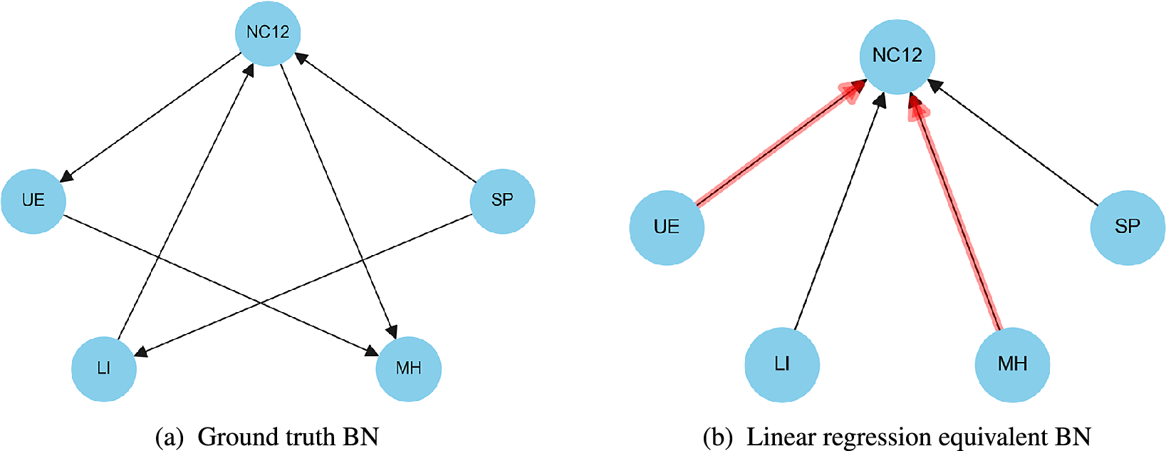
An example of a BN is given in Figure 1a with nodes depicting factors and directed edges indicating dependencies. For a given set of observations, which are a realization of factors generated from some underlying process, a BN or DAG encodes a set of conditional independencies. We note that the conditional independence structure of a set of factors does not uniquely define a causal path (Dawid, Reference Dawid, Guyon, Janzing and Schölkopf2010). However, they do provide a set of possible causal pathways, known as Markov equivalence classes, which can be causally distinguished from each other either by imposing prior knowledge or via intervention (Pearl et al., Reference Pearl2000).
(a) Bayesian network of a synthetic socioeconomic scenario. The factors of interest specify the nodes in the network, while the directed edges (arcs) indicate conditional dependence relationships between the nodes. (b) Linear regression model. The red edges indicate that the relationship between factors is found to be statistically significant using backwards variable selection.
2.1. Motivation
We motivate the use of BNs as a tool for policymakers wishing to understand the complex interaction between factors in a socioeconomic system by illustrating the limitations of linear regression, often used for the same purpose.
Figure 1a presents a hypothetical Bayesian Network representing a socioeconomic system. The variables in this network include family structure (Single Parent, $ SP $
), income levels (Low Income,
$ SP $
), income levels (Low Income, $ LI $
), educational attainment (Not Completed Year 12,
$ LI $
), educational attainment (Not Completed Year 12, $ NC12 $
), employment status (Unemployed,
$ NC12 $
), employment status (Unemployed, $ UE $
), and mental health (Mental Health,
$ UE $
), and mental health (Mental Health, $ MH $
). The network illustrates the following relationships: being a single parent (SP) influences both low-income (LI) and incomplete educational attainment (NC12). Subsequently, these factors impact employment status (UE) and mental health (MH).
$ MH $
). The network illustrates the following relationships: being a single parent (SP) influences both low-income (LI) and incomplete educational attainment (NC12). Subsequently, these factors impact employment status (UE) and mental health (MH).
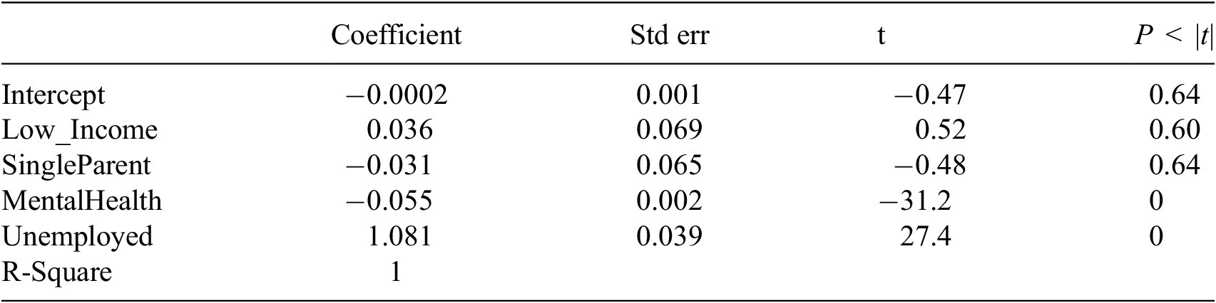
Figure 1b shows a BN representation of a linear regression model with the same factors. A linear regression model is a special case of a BN; one which has only one child and all the other factors are possible parents. In this instance, we assume that incomplete educational attainment is the response variable or child. To show the limitations of linear regression to model a network of interconnected factors, we generated data based on the relationships shown in Figure 1a and then analysed the impact of all the other factors on incomplete educational attainment, using backward variable selection for inference regarding the impact of factors on the outcome. The red lines in Figure 1b indicate relationships that were found to be statistically significant.
Figure 1b shows that linear regression fails to identify the true drivers (LI $ \to $
NC12) and (SP
$ \to $
NC12) and (SP $ \to $
NC12). This is not surprising because linear regression constrains the graph space,
$ \to $
NC12). This is not surprising because linear regression constrains the graph space, $ G $
, to those graphs where there is only one child, NC12 and all the other are possible direct parents as opposed to upstream ancestors. This constraint often results in misleading interpretations if one uses these techniques to infer dependencies between factors and perhaps explains why policies aimed at altering immediate causes, identified by regression analysis, for example, have not been successful in addressing societal issues. In contrast, BNs separate upstream dependencies from more immediate dependencies so that more nuanced and targeted interventions can be identified and implemented. In Section 3.2, Figure 3 shows how structure learning methods can recover the true data-generating process.
$ G $
, to those graphs where there is only one child, NC12 and all the other are possible direct parents as opposed to upstream ancestors. This constraint often results in misleading interpretations if one uses these techniques to infer dependencies between factors and perhaps explains why policies aimed at altering immediate causes, identified by regression analysis, for example, have not been successful in addressing societal issues. In contrast, BNs separate upstream dependencies from more immediate dependencies so that more nuanced and targeted interventions can be identified and implemented. In Section 3.2, Figure 3 shows how structure learning methods can recover the true data-generating process.
2.2. Learning the structure of a BN
Learning the structure of a BN from observational data is often referred to as causal discovery. Structure learning involves determining the optimal arrangement of nodes and edges in a BN from data. While the structure of a BN can provide valuable insights into the processes that generated that data and holds promise as a tool for policy formation, the task of learning the structure is proportionally difficult. There are two main reasons for this. First, the number of possible graph structures increases super exponentially with the number of nodes, making an exhaustive search over all possible graphs computationally infeasible, even for a modest number of nodes. Second, the space of graph structures is discrete, meaning that optimization methods that rely on gradients are not appropriate. In Bayesian structure learning, the problem becomes even more challenging because the goal is not only to find the optimal or most probable graph but also to attach probabilities to possible graphs. See Appendix B for technical details.
The structure of a graph encodes conditional independencies that exist among factors in a network, and Bayesian structure learning attaches probabilities to these conditional independence structures. However, graphs with the same conditional independence structures can have different causal interpretations, making predicting the impact of an intervention on an outcome problematic. To compute the likely impact of an intervention on an outcome, we can compute the impact of that intervention on all possible causal paths associated with an equivalence class, see Nandy et al. (Reference Nandy, Maathuis and Richardson2017).Footnote 2
3. Simulation study
This section builds upon the motivation example presented in Section 2.1, where we generated a dataset from a known DAG structure and applied a Linear Regression model to analyse the data. Synthetic data generation provides a controlled scenario where the causal structure is known, allowing us to systematically evaluate the performance of different modelling approaches. In that example, the Linear Regression failed to accurately identify the key relationships influencing the variable NotCompletedYear12, demonstrating the limitations of traditional regression models in capturing complex causal interactions and indirect effects. In this section, we are interested in understanding what factors influence the year $ 12 $
completion. To answer this question, present a simulated example to demonstrate the advantages of Bayesian structure learning over traditional optimization approaches that typically focus on identifying a single “best” DAG from observed data. By using Bayesian structure learning to represent uncertainty and multiple causally plausible models, we offer a more robust framework for policymaking that equips decision-makers with a richer set of potential causal explanations. These methods can enhance their ability to make more informed decisions in complex scenarios.
$ 12 $
completion. To answer this question, present a simulated example to demonstrate the advantages of Bayesian structure learning over traditional optimization approaches that typically focus on identifying a single “best” DAG from observed data. By using Bayesian structure learning to represent uncertainty and multiple causally plausible models, we offer a more robust framework for policymaking that equips decision-makers with a richer set of potential causal explanations. These methods can enhance their ability to make more informed decisions in complex scenarios.
3.1. Learning the best graph - PC algorithm
To understand the effectiveness of traditional optimization approaches that typically focus on identifying a single “best” DAG, we applied the PC Algorithm (Spirtes et al., Reference Spirtes, Glymour and Scheines2000) to learn the relationships among variables in the same synthetic dataset used in our Linear Regression example. The resulting graph is presented in Figure 2 together with an edge matrix that shows all the edges that the PC algorithm failed to identify when compared to the data generation DAG. Like other similar structure learning methods, the PC Algorithm demonstrated its limitations in accurately recovering the original data-generating graph. Specifically, it failed to identify four critical sets of relationships: $ LI\to NC12 $
,
$ LI\to NC12 $
, $ NC12\to UE $
,
$ NC12\to UE $
, $ SP\to NC12 $
, and
$ SP\to NC12 $
, and $ SP\to NC12 $
. This inability to capture the true causal structure highlights a fundamental challenge in structure learning models that commit to a single graph estimate.
$ SP\to NC12 $
. This inability to capture the true causal structure highlights a fundamental challenge in structure learning models that commit to a single graph estimate.
Comparison highlighting specific limitations in the PC algorithm’s ability to capture certain key relationships within the data. (left) Graph learned using the PC algorithm. (right) The difference between the edges in the predicted PC graph and the true graph.
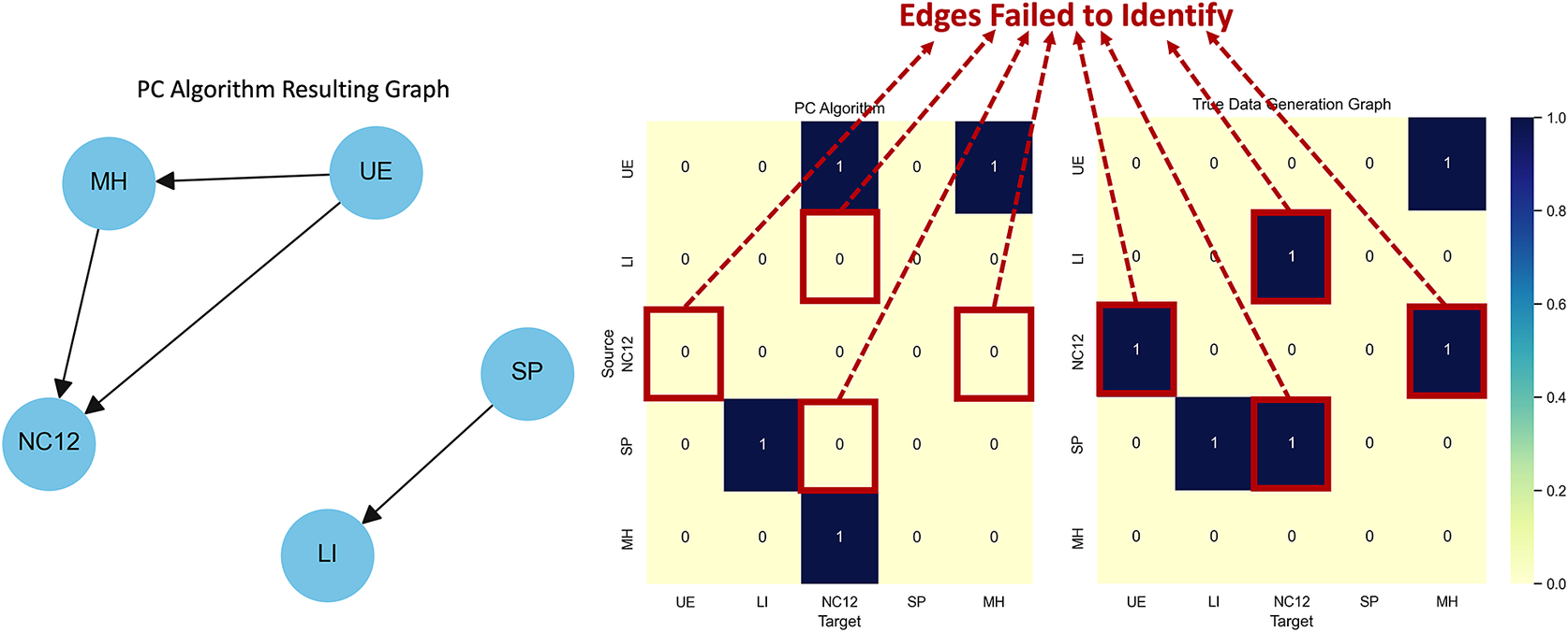
The PC Algorithm solely relies on conditional independence tests and assumes that the underlying graph is acyclic and faithful to the distribution of the data. However, its effectiveness is constrained by these assumptions and the quality of the conditional independence tests. As illustrated in our results, this often leads to incomplete or incorrect causal inferences, particularly in complex datasets where hidden variables and feedback loops may exist.
This limitation of the PC Algorithm underscores the necessity for more sophisticated inference methods that are capable of quantifying uncertainties both in the graph structure and its parameters. Such methods are important for developing robust and reliable policymaking tools that can adapt to the complexities and variabilities inherent in real-world data.
Probabilistic approaches, such as Bayesian structure learning, explore a range of possible graphs, providing a more nuanced and comprehensive understanding of potential causal connections. The reliance of the PC Algorithm on identifying a single, most likely graph overlooks other feasible—and potentially correct—outcomes, including those that more accurately reflect the true data-generating structure.
3.2. True posterior distribution analysis
Bayesian structure learning aims to quantify uncertainty by estimating the posterior probability distribution over all plausible DAGs. This posterior distribution encapsulates the degree of uncertainty regarding the various DAGs that could potentially explain the observed data. The primary objective of Bayesian structure learning is to quantify uncertainties by computing an approximate posterior distribution across all plausible DAGs rather than pinpointing a single ‘best’ graph.
An important concept in this context is that of equivalence classes. An equivalence class comprises multiple DAGs that encode the same set of conditional independencies. This means these equivalent classes cannot be distinguished from the data alone, as they represent statistically equivalent causal structures. Recognizing equivalence classes is important because different DAGs within the same class can suggest different causal interpretations, potentially leading to varying policy implications.
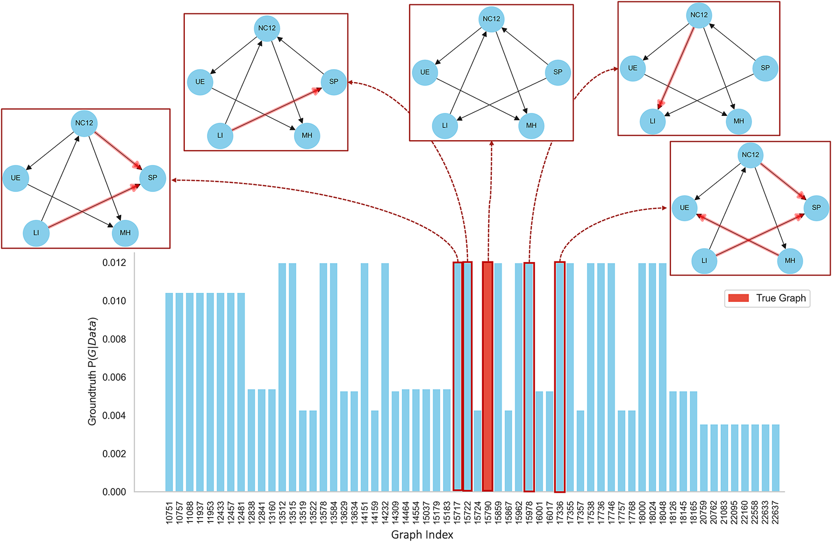
Figure 3 illustrates the posterior probability distribution for our synthetic data example. We generated this distribution by enumerating all possible DAGs for a five-node graph and evaluating each with a score function, specifically the BGe score (Heckerman et al., Reference Heckerman, Geiger and Chickering1995). The results show that while the true data-generating DAG is among those with the highest probabilities, there are 19 other DAGs with similar probabilities. These DAGs often feature reversed edges compared to the true graph, illustrating the variations in causal structures that can similarly explain the data.
This figure illustrates the probability distribution of Bayesian network structures as compared to the true graph. Among the networks analysed, there are 19 equivalent classes, each representing structures that exhibit identical conditional independencies. Four of these equivalent classes are emphasized, showcasing how their structures align with or differ from the true graph, providing insight into the robustness and variability within the network interpretations.
The main challenge lies in the vast number of possible DAGs that the algorithm needs to explore, even for relatively small datasets, which makes the computation impractical for large datasets (for a graph with only five variables, the space of DAGs is $ \mathrm{29,281} $
; for a six-node graph, this number explodes to
$ \mathrm{29,281} $
; for a six-node graph, this number explodes to $ \mathrm{3,781,503} $
). This means that we can no longer manually enumerate all possible DAGs in scenarios with more than five variables. For this, we will need advanced Bayesian structure learning algorithms, such as Partition MCMC (PMCMC), to approximate the true posterior distribution.
$ \mathrm{3,781,503} $
). This means that we can no longer manually enumerate all possible DAGs in scenarios with more than five variables. For this, we will need advanced Bayesian structure learning algorithms, such as Partition MCMC (PMCMC), to approximate the true posterior distribution.
3.3. Bayesian structure learning
In this section, we demonstrate the effectiveness of Bayesian structure learning algorithms by applying Partition MCMC (Kuipers and Moffa, Reference Kuipers and Moffa2017) for 300,000 iterations to our synthetic data example, which aligns with other works in the literature where 300,000 iterations are typically used for MCMC in similar causal discovery tasks (Cundy et al., Reference Cundy, Grover and Ermon2021). Figure 4 presents the recovered approximate posterior distribution, highlighting the graph structures most frequently visited by the algorithm. This distribution underscores the algorithm’s ability to explore a wide range of plausible graph structures, thus enhancing our understanding of the potential causal relationships within the data. Such understanding is important for making informed inferences about causal links in high-dimensional datasets, enabling researchers and policymakers to make decisions that are grounded in a detailed comprehension of the inherent uncertainties in the causal framework.
Comparative visualisation of Bayesian network structures inferred from PMCMC simulation. The bar chart displays the probability distribution of sampled networks, with the true network denoted in red, indicating the highest probability. Adjacency matrices compare edge occurrence probabilities from sampled DAGs against the true data generation graph, highlighting variances in edge predictions. Below, the predicted graphs with the highest scores are depicted, and the true graph is shown for reference.
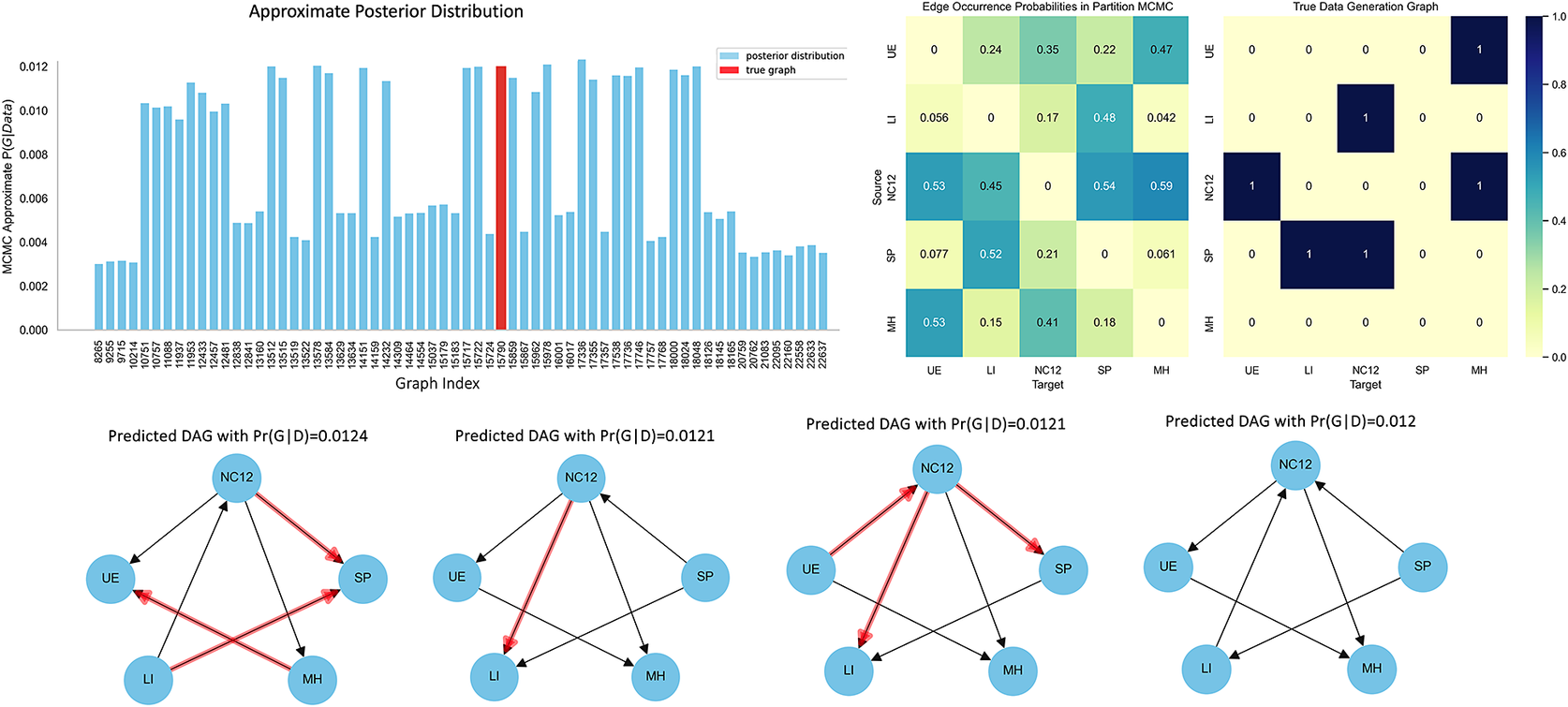
In Figure 4, the approximate posterior distribution shows a diverse set of DAGs, each suggesting different potential causal pathways within our dataset. This variety highlights the algorithm’s capability to explore the complex landscape of causal structures, suggesting that no single model dominates the posterior. This is particularly evident in the varied probabilities associated with the different DAGs shown, reflecting a significant level of uncertainty about the exact causal relationships. The edge occurrence probabilities. For example, the edge from $ UE\to NC12 $
exhibits a probability of 0.53, signifying a potential influence of unemployment on educational completion. Similarly,
$ UE\to NC12 $
exhibits a probability of 0.53, signifying a potential influence of unemployment on educational completion. Similarly, $ MH $
is shown to be influenced by
$ MH $
is shown to be influenced by $ NC12 $
with a probability of 0.59, suggesting that educational attainment might impact mental health outcomes. Note that the relationships with stronger probabilities align with those in the true data-generating DAG, indicating that the most frequently visited edges during the Bayesian learning process coincide with the actual data-generation DAG. This matrix enables us to quantify both the uncertainty and strength of each potential causal link, offering a detailed perspective on how various factors may interact within the system.
$ NC12 $
with a probability of 0.59, suggesting that educational attainment might impact mental health outcomes. Note that the relationships with stronger probabilities align with those in the true data-generating DAG, indicating that the most frequently visited edges during the Bayesian learning process coincide with the actual data-generation DAG. This matrix enables us to quantify both the uncertainty and strength of each potential causal link, offering a detailed perspective on how various factors may interact within the system.
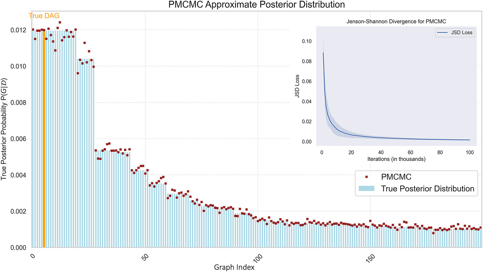
To analyse the convergence of the PMCMC algorithm, we employed the Jensen-Shannon Divergence (JSD) as a metric to measure the difference between the true posterior distribution, derived directly from the synthetic data and the PMCMC approximate distribution. The JSD is particularly useful in this context as it quantifies the similarity between two probability distributions, where a lower value indicates a closer match, thus reflecting a more accurate approximation by the algorithm (for mathematical details, refer to Appendix C). Additionally, to assess the robustness of our findings and quantify the uncertainty related to the generated dataset, we sampled five different datasets from the same true data-generating DAG and applied the PMCMC algorithm to each. This procedure allowed us to calculate the JSD across different samples for varying numbers of iterations. The consistent reduction in JSD across all samples further corroborates the efficacy of the PMCMC algorithm in diverse scenarios, enhancing our confidence in its use for exploring complex causal structures within high-dimensional datasets.
Figure 5 presents the JSD comparison between the true posterior probability distribution and the approximate posterior distribution obtained through PMCMC. In the figure, the red squares overlaying the blue bars indicate the posterior probabilities estimated by the PMCMC algorithm. These values are the algorithm’s approximation of how likely each DAG is to be the correct model based on the data. The analysis indicates that PMCMC performs well in approximating the true probabilities for the most likely DAGs. The performance appears to be particularly strong where the true probabilities are highest. As the index increases, both the true and approximated probabilities decline. This is typical in scenarios where a few models are much more likely than others, leading to a long tail of less likely models.
Comparison of True Posterior and PMCMC Approximate Posterior Distributions. This figure displays the true posterior probabilities (blue bars) and the PMCMC approximated probabilities (red squares) for a range of DAGs.
This empirical evidence reinforces the value of Bayesian structure learning, particularly using advanced algorithms like PMCMC, in uncovering the underlying causal dynamics within data. Such methods not only aid in achieving a deep understanding of the causal mechanisms but also provide a reliable foundation for making well-informed policy decisions that are crucial in dynamic and uncertain environments.
3.4. Discussion: towards policy decision-making using uncertainty quantification
Bayesian structure learning can enrich the understanding of policymakers who face the complex task of understanding and manipulating systems characterized by intricate and often conflicting causal structures by identifying and attaching probabilities to different causal pathways. This allows policymakers to better navigate the decision-making lifecycle, which typically includes agenda setting, policy formulation, adoption, implementation, and evaluation (Manski, Reference Manski2012). In addition, this process is able to adapt to new information and changing conditions so that policy decisions are both robust and timely.
3.4.1. Policy formulation
Bayesian structure learning can enable policymakers to identify the most relevant variables and their probable interconnections within a policy issue. For instance, in the context of unemployment and educational completion, understanding the strength and direction of influence can help prioritize areas that might benefit most from intervention. By presenting a range of plausible causal models, Bayesian methods allow for the definition of an agenda-setting process where multiple scenarios and their implications can be considered. The education data analysis from Section 3 illustrates this by highlighting how financial stability influences both health-related factors and school attendance. This allows policymakers to consider multiple pathways and potential interventions, such as addressing socio-economic disparities or improving health services, that can have ripple effects on educational outcomes.
3.4.2. Policy adoption and implementation
The detailed understanding of causal dynamics, provided by Bayesian structure learning, aids in the formation of policies that are most likely to achieve desired outcomes. For example, if data suggests a strong causal link between $ UE\to NC12 $
, interventions aimed at reducing unemployment can be prioritized in educational policy strategies. Furthermore, the ability to quantify uncertainty helps to identify information gaps and, therefore, can be used as an optimal real-time data acquisition strategy. In our education data analysis, for instance, quantifying the uncertainty in the relationship between
$ UE\to NC12 $
, interventions aimed at reducing unemployment can be prioritized in educational policy strategies. Furthermore, the ability to quantify uncertainty helps to identify information gaps and, therefore, can be used as an optimal real-time data acquisition strategy. In our education data analysis, for instance, quantifying the uncertainty in the relationship between $ LI $
and
$ LI $
and $ NC12 $
provides insights into areas where additional data could strengthen policy decisions, such as targeted interventions for financially vulnerable populations.
$ NC12 $
provides insights into areas where additional data could strengthen policy decisions, such as targeted interventions for financially vulnerable populations.
3.4.3. Policy evaluation
One of the main advantages of Bayesian structure learning in policymaking is its use in evaluating the effectiveness of a policy. In particular, Bayesian structure learning allows policymakers to evaluate the effect of a policy not only on a few outcomes but on the entire network of interconnected factors in a statistically rigorous manner. This is crucial for iterative policy processes, where ongoing evaluation feeds back into agenda-setting and policy formulation. In our example, we show how school attendance is influenced by education policies by factors such as mental health and financial stability. This allows for a comprehensive evaluation of how a policy, like supporting mental health services, indirectly impacts educational outcomes, helping policymakers adapt their strategies based on real-time evaluations.
3.4.4. Enhancing robustness and resilience
Utilizing Bayesian structure learning also enhances the robustness and resilience of policies by preparing policymakers to handle various potential future scenarios. The method’s ability to provide a comprehensive view of possible outcomes and their probabilities supports the development of contingency plans and adaptive strategies, ensuring policies remain effective under different future conditions. Our case study on school attendance demonstrates how interventions focused solely on educational inputs may fail if upstream factors, such as health or financial challenges, are not addressed. By considering multiple causal pathways and their associated probabilities, policymakers can develop more resilient strategies adaptable to changing conditions.
In conclusion, Bayesian structure learning enhances policymaking by providing a more data-informed and adaptive process. It empowers policymakers with a toolkit for rigorous analysis and decision-making, capable of handling the uncertainties and complexities inherent in modern policy environments. This approach can potentially enhance the effectiveness of policies and increase transparency and accountability in decision-making processes (Alzubaidi et al. Reference Alzubaidi, Al-Sabaawi, Bai, Dukhan, Alkenani, Al-Asadi, Alwzwazy, Manoufali, Fadhel and Albahri2023; Chou Reference Chou, Moreira, Bruza, Ouyang and Jorge2022; Velmurugan Reference Velmurugan, Ouyang, Moreira and Sindhgatta2021), fostering a deeper trust in public institutions.
4. Application: student school attendance
This case study shows how causal discovery for BNs can be employed to unpack complex dependencies and suggest likely causal relationships between frequent school absence and student and family characteristics. It illustrates how causal discovery stratifies the dependencies between factors that may impact school attendance into proximal and upstream causes and, by doing so, offers insights into which policies are optimal in order to address the issue. We also show how to estimate the effect of various interventions while accounting for the uncertainty over possible causal pathways, which can help inform decisions.
4.1. Dataset description
The dataset is derived from ‘Growing Up in Australia: The Longitudinal Study of Australian Children (LSAC) (Mohal et al., Reference Mohal, Lansangan, Gasser, Taylor, Renda, Jessup and Daraganova2021), a nationwide longitudinal project that examines social, economic, physical, and cultural factors influencing children’s health, learning, and overall developmental trajectories. The study tracks the growth and developmental milestones of two primary cohorts: a birth (B) cohort, which contains information on 5107 children who were aged less than 1 year in 2004, and the kindergarten (K) cohort, consisting of 4983 children who were between the ages of four and five in 2004. Spanning from 2004 through 2016, the LSAC contains data across seven biennial waves. Informed by discussions with domain experts in education, we constructed 12 binary variables based on the extensive LSAC questionnaires:
-
1. Financial Stability (FS): Families financial position covered by item fn06a from the LSAC data asset. All responses above “Reasonably comfortable” are labelled as positive in the binary setting.
-
2. Parents Not Employed (NE): When both parents are not employed for dual-parent families or when one parent is not employed for single-parent families. Based on items aemp and bemp of LSAC.
-
3. Parent 1 Alcohol Abuse (AA): Defined as having heavy daily alcohol consumption (>4 drinks for men >2 for women) or frequent binge drinking (7+ drinks in a sitting for men 5+ for women 2 to 3 times a month or more often). Based on item aalcp of LSAC.
-
4. Parent Communication (COMM): Arising from the construct of parental involvement and defined as positive when there is daily communication between the parent(s) study child. Based on item he11a1a of LSAC.
-
5. Sleep Problems (SP) Defined as having a sleep problem, such as wheezing, coughing, not sleeping alone, night-walking, or restless sleep, for 4 or more nights a week. Based on item hs20b of LSAC.
-
6. General Health (GH) Based on item hs13c of LSAC, it is a measure of global health reported by the parents and identified as positive when responses are above “Very Good.”
-
7. Watches TV (TV) A measure of the amount of time spent watching TV constructed from variable he06b2 in LSAC and considered as positive when the watching time exceeds 1 hour per day.
-
8. Ongoing Medical Condition (OMC) Depicts if the child has any ongoing health condition (no need for them to be diagnosed) that is present for some period of time or re-occur regularly. These include hearing problems, developmental delay, eczema, diarrhoea, infections and other illnesses. Based on variable hs17 from LSAC.
-
9. Learning Disability (LD) Reported by the parents and identified as a specific difficulty learning or understanding things by the child. Based on variable f17em1 of LSAC.
-
10. Physical Condition (PC) Reported by the parents as any condition restricting physical activity or work. Based on variable f17im1 in LSAC.
-
11. School Enjoyment (SE) Defined as positive when the study child reports looking forward to going to school most days and based on pc29a of LSAC.
-
12. School Absence Frequent (SAF) Reported by the child’s teacher as a binary measure of frequent school absences. Based on variable pc48t1b of LSAC.
We have selected all observations across waves and cohorts where these variables are measured to obtain a wider view of the relationships between these. A data pre-processing stage consisted of binarising originally ordinal variables and deleting records with missing data, resulting in 20,890 observations from all 10,090 unique individuals for this sample. We stress that this real example is used as a proof of concept only and note that the causal pathways which lead to school absence are likely to be heterogeneous, both with respect to time and with respect to sub-population characteristics.
4.2. Results
Similar to Section 3.3, we adopt a Bayesian approach and use Partition MCMC to infer the structure of a BN from observational data while quantifying the uncertainty over possible structures. We allowed the estimation algorithm to run for 100,000 iterations and utilised the BDe score (Heckerman and Geiger, Reference Heckerman and Geiger2013).
Figure 6 shows the Maximum A Posteriori (MAP) structure, most likely the structure given the data. A key advantage of DAGs is that they can be used to represent causal diagrams, where causal relationships among variables can be suggested and inferred. We emphasise suggested since it is well known that observational data alone cannot distinguish causality from association (Spirtes et al., Reference Spirtes, Glymour and Scheines2000). The MAP graph estimates in Figure 6 depict the relationships among many factors. This structure shows many complex relationships and interactions to analyse and reason about, which becomes the main point of collaboration and discussion between mathematicians, computer scientists and policymakers. We first start by highlighting general insights from this graph and later move into a comparison with other techniques, such as logistic regression.
The Maximum A Posteriori (MAP) DAG, based on the LSAC dataset, features the ‘School Absence Frequent’ node emphasised with a red diamond. The edge coefficients are derived from the data according to the most probable DAG obtained with Partition MCMC. Blue edges represent positive correlations, while orange edges signify negative correlations. Ancestor nodes of ‘School Absence Frequent’ are marked with orange ellipses.
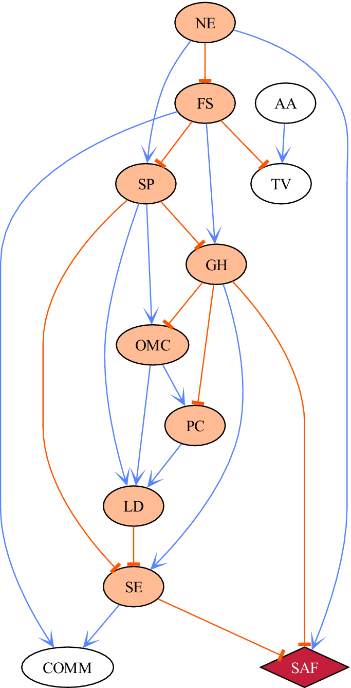
Figure 6 shows the network of factors that contribute directly or indirectly to frequent school absence (SAF), which is highlighted as a red node with a diamond shape. The nodes that are ancestors of SAF, that is, those that are connected directly or indirectly to the outcome, are coloured in orange. At the top of the hierarchy is employment, represented by the variable Not in Employment (NE), which is negatively linked with the Financial Stability (FS) of the family and positively related to Sleep Problems (SP) and SAF. Both NE and FS are the main factors that affect the child’s Sleep Problems (SP) and impact many areas, including Ongoing Medical Condition (OMC), Learning Disability (LD), School Enjoyment (SE) and General Health (GH). GH is not surprisingly negatively related to OMC. GH is also positively related to SE, which is directly connected to school absence, with an increase in SE associated with a decrease in SAF.
Following Section 3, we compare the inference regarding the factors that impact school absence obtained using a BN with that obtained using logistic regression. As noted previously, a regression model is a special case of a BN - one in which there is only one child and all other factors are potential direct parents, and this constraint can lead to different inferences. The coefficients for the resulting logistic regression model are presented in Appendix D, Table D1. There are interesting similarities between both techniques. Specifically, the two most important factors associated with school absence are GH and SE. Logistic regression also identifies the statistically significant dependencies on school absence from SP, FS and NE. However, due to the constraints implicit in regression models, inference from this logistic regression model can be very misleading. It particularly presents statistically significant relationships between school absence and AA and TV, which might co-vary if assumed independent, but our approach, which considers and explores possible interactions, deems these not part of the causal pathways towards school absence. Further evidence of the limitations of logistic regression models in this setting is exposing those relationships that are missed, such as the influence of learning disabilities (LD), which is flagged as non-statistically significant by logistic regression but that when using Bayesian inference over DAGs is recognised as an influencing factor for school enjoyment which in turn decreases school absence.
4.3. Implications for policymaking
As discussed in Section 2.1, a key advantage of BNs over other data-driven techniques used for policymaking is the ability to represent a set of complex factors as an easy-to-interpret network of stratified factors. This stratification has important implications for policymakers. In this example, one of the proximal causes of school absence is school enjoyment, which, in turn, depends upon a child’s general health and sleeping patterns. Both health and sleep, in turn, depend upon the family’s financial stability. There are many current programs with the goal of increasing school enjoyment and, therefore, increasing attendance. However, this simple example shows that while such programs may help, impacts from these programs are likely to be unsustainable if upstream causes such as financial stability, sleep, and health are not addressed. Indeed, this analysis partially explains why policies aimed at altering immediate causes alone, leaving the root causes untouched, have failed to address entrenched societal issues, such as lack of school engagement. From an education-specific perspective, this analysis shows that policies that target the “in-school” causes will not be enough if causes “outside school” are not also tackled. For example while Figure 6, shows that the proximate causes of frequent school absence are school enjoyment and general health, these are affected by the financial stability and employment of the family as well as the child’s quality of sleep. This suggests that any policy aimed at targeting school enjoyment is unlikely to have a sustained effect on school attendance if upstream causes are not also addressed.
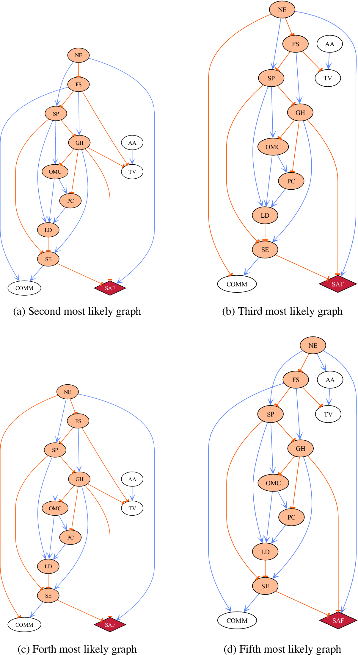
Appendix E shows the next four most probable graphs (after the MAP graph in Figure 6). These five most probable graphs account for 80% of the probability mass and are remarkably similar. All show that financial stability, parental employment and sleep are the upstream causes of frequent school absence. These upstream factors lead to adverse health outcomes which in turn effect school enjoyment and attendance. The concordance of these graphs indicates that the uncertainty surrounding the causal factors behind school attendance, for this dataset, is low.
Ensuring data privacy can be addressed through careful data management and the application of anonymisation techniques, ensuring that sensitive information is protected while still enabling the extraction of valuable insights.
5. Challenges and considerations
Several barriers may impede the adoption of Bayesian approaches in policymaking. One significant challenge is the complexity of Bayesian models, which can be difficult for non-experts to understand and implement. This complexity necessitates a level of statistical literacy and familiarity with Bayesian principles that may not be common among policymakers. Additionally, the computational demands of Bayesian structure learning, especially in large-scale applications, can be substantial. High computational costs and the need for specialized software and expertise may limit the practical implementation of these methods in policy environments with constrained resources.
Data quality and availability also pose challenges. Bayesian methods rely heavily on high-quality, comprehensive data to generate accurate models. In many policy domains, data may be incomplete, biased, or outdated, which can undermine the reliability of the resulting models, and the policy decisions based on them. Ensuring data privacy and security while integrating diverse data sources adds another layer of complexity.
An additional consideration for policymakers is the concept of equivalence classes in Bayesian structure learning. Different DAGs within the same equivalence class encode the same set of conditional independencies but have different causal interpretations. Therefore, it is crucial for policymakers to recognize that the data alone may not uniquely determine the directionality of some causal relationships. This ambiguity can potentially lead to incorrect conclusions and misguided policy decisions if not properly addressed. To mitigate this risk, policymakers need to incorporate expert knowledge or interventional data to more precisely identify the true causal structures.
Incorporating probabilistic frameworks into policymaking requires a significant shift in mindset for politicians, civil servants, and the voting public. This shift involves moving from deterministic thinking to an understanding that policy decisions should be based on the likelihood of various outcomes and their potential impacts. Embracing this probabilistic approach allows more informed and flexible decision-making, particularly in complex and uncertain environments. However, effectively interpreting and utilising probabilistic models requires technical knowledge. Policymakers and their advisors must be equipped with the necessary skills to understand and apply these models. This underscores the importance of capacity building and education in statistical concepts, probability theory, and data interpretation.
Despite these barriers, adopting Bayesian approaches in policymaking equips policymakers with powerful tools to navigate the complexities and uncertainties inherent in socioeconomic systems. Bayesian methods foster more informed, transparent, and accountable decisions by providing clear, interpretable models that incorporate uncertainty and multiple causal pathways. This leads to more effective and adaptive policies that can better meet the needs of society, even in the face of changing conditions and unforeseen challenges. Embracing Bayesian networks and causal discovery represents a significant step forward in the quest for evidence-based, resilient policymaking.
6. Conclusion
This paper presented an approach to integrate structure learning and causal discovery into policy decision-making. Through our case studies — one using synthetic data and the other applying these methodologies to educational data, we demonstrated the potential of these advanced statistical machine-learning techniques in addressing complex policy issues, particularly for education. By leveraging the power of Bayesian methods, policymakers can gain a more comprehensive understanding of the policy landscape, which is crucial for developing strategies that are both effective and adaptable to changing conditions.
Our approach integrates causal discovery within a Bayesian framework, which allows for the consideration of multiple possible causal pathways rather than focusing solely on the most likely one. This is particularly relevant in complex decision landscapes where multiple near-equally likely pathways may exist. The application of Bayesian networks in this context helps quantify uncertainty, providing policymakers with a probabilistic understanding of potential outcomes and the risks associated with different policy interventions.
Ultimately, the adoption of Bayesian approaches in policymaking equips policymakers with a powerful set of tools to navigate the complexities and uncertainties inherent in socioeconomic systems. By providing clear, interpretable models that incorporate uncertainty and multiple causal pathways, Bayesian methods foster more informed, transparent, and accountable decisions. This leads to more effective and adaptive policies that can better meet the needs of society, even in the face of changing conditions and unforeseen challenges. Embracing Bayesian networks and causal discovery represents a significant step forward in the quest for evidence-based, resilient policymaking.
Abbreviations
- BN
-
Bayesian Network
- MCMC
-
Markov Chain Monte Carlo
- DAG
-
Directed Acyclical Graph
Data availability statement
The source code and simulated data used in this project are available at https://github.com/human-technology-institute/bayesian-causal-policy. The LSAC dataset can be accessed for research purposes through the Australian Data Archive at https://dataverse.ada.edu.au/dataverse/lsac.
Acknowledgements
We acknowledge the research assistance contribution of Linduni Rodrigo by providing support for the analysis of the LSAC dataset and Rebekah Grace, Susan Collings and Daniel Waller from the University of Western Sydney for vivid discussions around the inclusion of relevant factors to understand student school attendance and the relevance of student attendance on long-lasting individual outcomes.
Author contributions
Conceptualization: all authors; Data curation: C.M., N.L.C.N. and R.M; Formal analysis: C.M., N.L.C.N. and R.M; Funding acquisition: S.C. and R.M.; Investigation: all authors; Methodology: all authors; Project administration: R.M.; Software: C.M., N.L.C.N. and R.M; Supervision: C.M., R.M. and S.C.; Validation: C.M., N.L.C.N. and R.M; Visualization: C.M., N.L.C.N. and R.M; Writing—original draft: C.M., N.L.C.N. and R.M.; Writing—review and editing: all authors.
Funding statement
This research was supported by the Paul Ramsay Foundation (PRF) under the Thrive: Finishing School Well program. The funders had no role in study design, data collection and analysis, decision to publish, or manuscript preparation.
Competing interest
The authors declare no competing interests.
A. Linear regression output
OLS summarised results
B. Bayesian structure learning
This appendix section outlines the fundamental concepts of structure learning. It begins with an introduction to Bayesian networks, covering the foundational theory and their advantages for decision-making over other machine learning algorithms. It then explores the structure learning process within these networks, detailing the mathematical methods used to estimate network structures from data.
B.1. Bayesian networks
Bayesian Networks (BNs), also known as Bayes nets, belief networks, or decision networks, are probabilistic graphical models that provide an effective framework for multivariate statistical modelling, allowing for better representation and understanding of complex relationships amongst variables of interest. A BN is defined by a graph $ \mathcal{G} $
, which is a tuple of
$ \mathcal{G} $
, which is a tuple of $ \left\{\mathcal{V},\mathrm{\mathcal{E}}\right\} $
, where
$ \left\{\mathcal{V},\mathrm{\mathcal{E}}\right\} $
, where $ \mathcal{V} $
is a set of
$ \mathcal{V} $
is a set of $ n $
nodes, where node
$ n $
nodes, where node $ i $
in the graph represents a random variable
$ i $
in the graph represents a random variable $ {X}_i $
; and where
$ {X}_i $
; and where $ \mathrm{\mathcal{E}} $
is the set of edges that connect two nodes, indicating a causal relationship between these two nodes with the strength of this relationship characterised by a parameter for each edge.
$ \mathrm{\mathcal{E}} $
is the set of edges that connect two nodes, indicating a causal relationship between these two nodes with the strength of this relationship characterised by a parameter for each edge. $ \mathcal{G} $
is a DAG, where all edges have directions, and no cycles are present. The directional property in edges allows us to define a hierarchical relationship between nodes, e.g., an edge from a node
$ \mathcal{G} $
is a DAG, where all edges have directions, and no cycles are present. The directional property in edges allows us to define a hierarchical relationship between nodes, e.g., an edge from a node $ i $
to node
$ i $
to node $ j $
,
$ j $
, $ {X}_i\to {X}_j $
, means that
$ {X}_i\to {X}_j $
, means that $ {X}_i $
belongs to the parent set of node
$ {X}_i $
belongs to the parent set of node $ j $
,
$ j $
, $ {\mathrm{Pa}}_j $
; and
$ {\mathrm{Pa}}_j $
; and $ {X}_j $
is a child of node
$ {X}_j $
is a child of node $ i $
.
$ i $
.
One important feature of a BN is that each variable is conditionally independent of the set of all its predecessors, given the states of its parents. Therefore, the joint probability distribution of the nodes can be written as a product of the conditional distributions, each of which only depends on its parents in the graph,
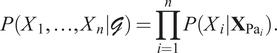 $$ P\left({X}_1,\dots, {X}_n|\mathcal{G}\right)=\prod \limits_{i=1}^nP\left({X}_i|{\mathbf{X}}_{{\mathrm{Pa}}_i}\right). $$
For discrete random variables, the dependencies can be quantified using Conditional Probability Tables (CPTs), which specify the probability of each variable value given its parents’ values and reflect the strength of the relationships between the variables in the network Koller and Friedman (Reference Koller and Friedman2009); Pearl (Reference Pearl1988).
BNs offer several advantages for decision-making compared to classical machine learning methods such as neural networks, support vector machines, regressions, and so forth They offer rich semantic meaning and can be readily comprehended by users without extensive statistical expertise. They facilitate effective learning from data to construct a model that provides a good approximation to our past experience, exploring connections between variables, and providing novel insights about a domain that can be utilised to assist informed decision-making, which can be particularly useful in areas such as educational and institutional research Fernández et al. (Reference Fernández, Morales, Rodríguez and Salmerón2011).
B.2. Structure learning
Learning a BN involves both estimating the structure $ \mathcal{G} $
(structure learning) and its associated set of parameters
$ \mathcal{G} $
(structure learning) and its associated set of parameters $ \Theta $
(parameter learning). While parameter learning is straightforward given the estimated structure since it can be treated as a standard regression problem, structure learning of BNs is challenging due to (i) the super-exponential growth of possible graph structures with the increasing number of nodes in the network and (ii) the discrete parameter space prohibiting gradient-based methods from being utilised in solving this problem.
$ \Theta $
(parameter learning). While parameter learning is straightforward given the estimated structure since it can be treated as a standard regression problem, structure learning of BNs is challenging due to (i) the super-exponential growth of possible graph structures with the increasing number of nodes in the network and (ii) the discrete parameter space prohibiting gradient-based methods from being utilised in solving this problem.
While traditional methods focus on recovering a single plausible graph or its Markov equivalence, the Bayesian approach to structure learning aims to infer a full posterior distribution over graphs, enabling effective use of Bayesian model averaging for inference in high dimensional domains with sparse data, where no single best model can be clearly identified. The posterior probability of a DAG $ \mathcal{G} $
given the data
$ \mathcal{G} $
given the data $ \mathcal{D} $
is used as its score and can be derived from Bayes’ theorem
$ \mathcal{D} $
is used as its score and can be derived from Bayes’ theorem
 $$ P\left(\mathcal{G}|\mathcal{D}\right)\propto P\left(\mathcal{D}|\mathcal{G}\right)P\left(\mathcal{G}\right), $$
where $ P\left(\mathcal{G}\right) $
denotes a prior distribution over the graph structures and
$ P\left(\mathcal{G}\right) $
denotes a prior distribution over the graph structures and $ P\left(\mathcal{D}|\mathcal{G}\right) $
refers to the marginal likelihood derived by marginalising out the parameter
$ P\left(\mathcal{D}|\mathcal{G}\right) $
refers to the marginal likelihood derived by marginalising out the parameter $ \Theta $
. This can be achieved by integrating the parameters
$ \Theta $
. This can be achieved by integrating the parameters
 $$ P\left(\mathcal{D}|\mathcal{G}\right)=\int P\left(\mathcal{D}|\Theta, \mathcal{G}\right)P\left(|\mathcal{G}\right)d, $$
where $ P\left(\Theta |\mathcal{G}\right) $
is a prior distribution for the parameter
$ P\left(\Theta |\mathcal{G}\right) $
is a prior distribution for the parameter $ \Theta $
given the graph
$ \Theta $
given the graph $ \mathcal{G} $
.
$ \mathcal{G} $
.
A general Bayesian scoring metric can be decomposed when the data is complete, and the conditions of structure modularity, parameter modularity, and parameter independence for the prior distributions are satisfied Heckerman and Geiger (Reference Heckerman and Geiger2013): $ P\left(\mathcal{D}|\mathcal{G}\right)={\prod}_i\;S\left({X}_i,{\mathbf{Pa}}_i\right) $
, with
$ P\left(\mathcal{D}|\mathcal{G}\right)={\prod}_i\;S\left({X}_i,{\mathbf{Pa}}_i\right) $
, with $ S\left(\cdot \right) $
representing the score function that depends on the node
$ S\left(\cdot \right) $
representing the score function that depends on the node $ {X}_i $
and its corresponding parents. This is essential for effective implementation, as it reduces the structure search in an iteration to only reevaluating the nodes with changes in their parents compared to the previously scored structure. Since exhaustive search is impractical even with only a modest number of nodes due to the space of all possible DAG structures as the number of variables increases, approximate solutions can be achieved via Markov chain Monte Carlo (MCMC) (Kuipers and Moffa, Reference Kuipers and Moffa2017) or variational methods.
$ {X}_i $
and its corresponding parents. This is essential for effective implementation, as it reduces the structure search in an iteration to only reevaluating the nodes with changes in their parents compared to the previously scored structure. Since exhaustive search is impractical even with only a modest number of nodes due to the space of all possible DAG structures as the number of variables increases, approximate solutions can be achieved via Markov chain Monte Carlo (MCMC) (Kuipers and Moffa, Reference Kuipers and Moffa2017) or variational methods.
C. Metrics
Understanding the strengths and limitations of MCMC and other inference tools is essential for practitioners and policymakers when interpreting results and translating them into policy. To gain insight into the performance of the MCMC algorithm, we inspect its algorithmic convergence by comparing the true posterior distribution with the approximate distribution using the Jensen-Shanon Divergence (JSD).
The JSD metric measures the similarity between two probability distributions. Mathematically, the JSD between two probability distributions $ P $
and
$ P $
and $ Q $
is defined as
$ Q $
is defined as
 $$ JSD\left(P\Big\Vert Q\right)=\frac{1}{2} KL\left(P\Big\Vert M\right)+\frac{1}{2} KL\left(Q\Big\Vert M\right)\hskip1.08em \mathrm{where}\hskip0.48em M=\frac{1}{2}\left(P+Q\right), $$
and $ KL\left(P\Big\Vert M\right) $
and
$ KL\left(P\Big\Vert M\right) $
and $ KL\left(Q\Big\Vert M\right) $
are the Kullback–Leibler (KL) divergences of
$ KL\left(Q\Big\Vert M\right) $
are the Kullback–Leibler (KL) divergences of $ P $
and
$ P $
and $ Q $
from
$ Q $
from $ M $
, respectively. The KL is given by
$ M $
, respectively. The KL is given by
 $$ KL\left(P\Big\Vert M\right)=\sum \limits_iP(i)\log \left(\frac{P(i)}{M(i)}\right), $$
with $ i $
indexes all possible DAGs for
$ i $
indexes all possible DAGs for $ n $
nodes.
$ n $
nodes.
We also measured how the entropy of the true and approximate distributions varied with the amount of generated data points. Entropy provides a measure of the uncertainty or unpredictability of the distribution. Higher entropy means the distribution is more spread out and less certain, while lower entropy means the distribution is more peaked and predictable. The entropy $ H $
of a discrete set of probabilities
$ H $
of a discrete set of probabilities $ \left\{{p}_1,{p}_2,\dots, {p}_n\right\} $
is defined as
$ \left\{{p}_1,{p}_2,\dots, {p}_n\right\} $
is defined as
 $$ H(P)=-\sum \limits_{i=1}^n\;{p}_i{\log}_2\left({p}_i\right). $$
D. Logistic regression for frequent school absence
As part of the comparison with other baseline modelling strategies, we have also estimated a logistic regression model to the LSAC data using the same variables as in Section 4. Table D1 presents a summary of the individual coefficients and their value, including the p-value associated with individual variables.
Expected value and standard deviation for coefficients of a logistic regression model which assumes independent and direct influence of all factors over School Absence
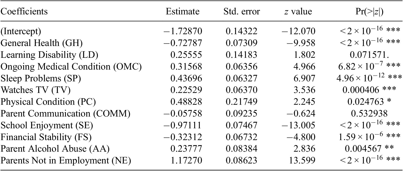
Note. The significance codes indicate the level of statistical significance: ‘***’ indicates p < 0.001, ‘**’ indicates p < 0.01, ‘*’ indicates p < 0.05, ‘.’ indicates p < 0.1, and ‘’ (blank) indicates p $ \ge $
0.1
$ \ge $
0.1
E. Uncertainty quantification over graph structures for school attendance
As explained in Section B.2, the resulting estimation of graphs is a posterior probability distribution in the space of DAGs, $ \mathcal{G} $
. The process of causal discovery using MCMC generates a Markov chain which approximates the full posterior distribution, where the number of times each graph appears in the chain is proportional to its posterior probability. The variability in the graphs part of this posterior distribution is a measure of uncertainty over the graph structures.
$ \mathcal{G} $
. The process of causal discovery using MCMC generates a Markov chain which approximates the full posterior distribution, where the number of times each graph appears in the chain is proportional to its posterior probability. The variability in the graphs part of this posterior distribution is a measure of uncertainty over the graph structures.
The results produced in Section 4.2, the 100,000 iterations result in 276 unique graph structures. The top 5 structures accumulate 80% of the full probability mass and are very similar. The next 4 most probable graph structures are shown in Figure E1.
Top graphs, following the MAP graph (Figure 6), in the posterior distribution.


 Open access
Comments
No Comments have been published for this article.