


INTRODUCTION
Crevasses are commonly observed on ice bodies and have far-reaching implications for glacier dynamics. Given temperate conditions, fracture networks in the ice route surficial meltwater to the glacier base or store it englacially (e.g., Fountain and Walder, Reference Fountain and Walder1998). At the bottom of a glacier, basal crevasses can extend the subglacial drainage system some tens of meters into the ice (Harper and others, Reference Harper, Bradford, Humphrey and Meierbachtol2010). The process of crevassing affects glacial hydrology which, in turn, is crucial for ice flow dynamics (e.g., Iken and Bindschadler, Reference Iken and Bindschadler1986; Flowers and Clarke, Reference Flowers and Clarke2002). In addition, by providing water pathways, crevasses promote cryohydraulic warming, thus softening the ice and influencing ice flow (Phillips and others, Reference Phillips, Rajaram and Steffen2010). Apart from its implications for ice flow, fracturing increases the ice damage state (Pralong and Funk, Reference Pralong and Funk2005) and may lead to structural failure of the ice. This may be observed for example, as ice avalanching (e.g., Röthlisberger, Reference Röthlisberger1977), rapid drainage of ice-dammed lakes (e.g., Das and others, Reference Das2008), or iceberg calving (Benn and others, Reference Benn, Warren and Mottram2007). Colgan and others (Reference Colgan2016) provide a comprehensive discussion on the role of crevasses.
Surface crevasses can be remotely mapped and monitored using visual imagery (Krimmel and Meier, Reference Krimmel and Meier1975) or radar imagery (Fahnestock and others, Reference Fahnestock, Bindschadler, Kwok and Jezek1993). However, coarse resolution and snow cover complicate this analysis. Additionally, limited radar penetration depth prohibits the detection of englacial fractures. To investigate the latter, various geophysical methods such as borehole analysis (e.g., Harper and others, Reference Harper, Bradford, Humphrey and Meierbachtol2010), ground penetrating radar (e.g., Jezek and Bentley, Reference Jezek and Bentley1979) and active-source seismics (e.g., Navarro and others, Reference Navarro, Macheret and Benjumea2005) have been employed. Bradford and others (Reference Bradford, Nichols, Harper and Meierbachtol2013) investigated basal crevasses by means of anisotropy in electromagnetic and seismic wave velocities caused by the preferential alignment of the crevasses. Vertical fractures in an otherwise homogeneous ice body lead to a transversely isotropic medium with a horizontal axis of symmetry (or horizontal transversely isotropic) which is subject to azimuthal anisotropy in seismic wave propagation (Crampin and others, Reference Crampin, McGonigle and Bamford1980; Bakulin and others, Reference Bakulin, Grechka and Tsvankin2000). Apart from azimuthal anisotropy, the presence of crevasses may lead to band gaps in elastic wave propagation (Freed-Brown and others, Reference Freed-Brown, Amundson, MacAyeal and Zhang2012).
Recently, passive seismology has complemented other geophysical methods in the cryospheric sciences (Podolskiy and Walter, Reference Podolskiy and Walter2016; Aster and Winberry, Reference Aster and Winberry2017). Passive seismology is mainly used to investigate processes within a medium such as englacial fracturing (Neave and Savage, Reference Neave and Savage1970; Walter and others, Reference Walter, Dreger, Clinton, Deichmann and Funk2010), subglacial water flow (Bartholomaus and others, Reference Bartholomaus2015; Gimbert and others, Reference Gimbert, Tsai, Bartholomaus, Jason and Walter2016), or stick-slip ice motion (Weaver and Malone, Reference Weaver and Malone1979; Winberry and others, Reference Winberry, Anandakrishnan, Wiens, Alley and Christianson2011) by analyzing the seismic waves emitted by these processes. Apart from source studies, passive seismology also allows to characterize the physical properties of the medium (Zhan and others, Reference Zhan, Tsai, Jackson and Helmberger2013; Diez and others, Reference Diez2016). This is also done using active-source seismics. Compared with active-source seismics, passive seismology is less laborious and allows the recording of long and continuous time series at the same time. Continuous recording modes, in turn, allow for monitoring the time evolution of seismic activity and changes in the medium properties.
In this study, we use the signal from naturally occurring icequakes on Glacier de la Plaine Morte, Switzerland (Fig. 1a), to investigate the variation of seismic wave velocity as a function of propagation direction. In particular, we study Rayleigh-wave azimuthal anisotropy in regions with preferential alignment of crevasses and establish a relationship between the two. In the following sections, we first describe our 2016 field campaign and the data collected. This is followed by our processing scheme to locate icequakes, and to determine the frequency-dependent Rayleigh-wave phase velocities using beamforming. We find significant azimuthal anisotropy and discuss their causes.
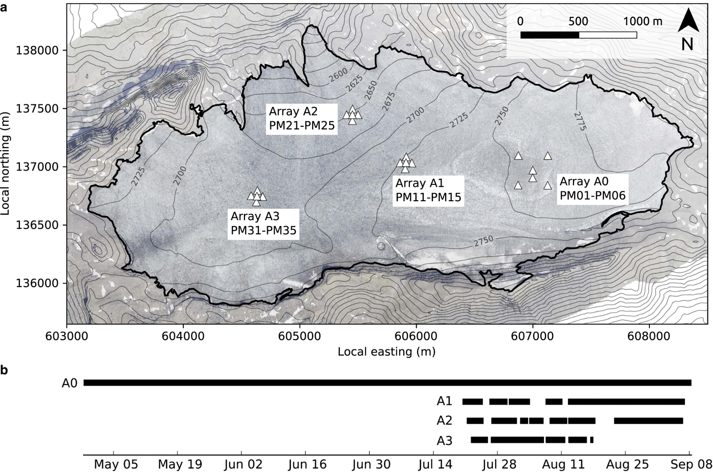
(a) Map with surface topography of Glacier de la Plaine Morte. The thick black line indicates the glacier extent and the white triangles show the locations of the seismic stations. In the background, an orthophotograph is shown. Aperture of array A0 with stations PM01-PM06 is 360 m, apertures of arrays A1 (PM11-PM15), A2 (PM21-PM25) and A3 (PM31-PM35) are 100 m. Stations are numbered for each array counterclockwise from 1 (North; Northeast for A0) to 5 (center station). Station PM06 (lower center station of A0) was added late, that is, in August. Coordinates of the Swiss Grid are shown. (b) Data availability of the stations in 2016. Black bars indicate times when all stations of an array were operational (station PM06 not considered for this illustration). Only times where at least two arrays were fully operational are considered in this study.
FIELD SITE
With an extent of ~7.5 km2, Glacier de la Plaine Morte in Switzerland (Fig. 1a) is the largest plateau glacier in the European Alps. More than 90% of its surface occupies the narrow elevation range between 2650 and 2800 m.a.s.l. (Huss and others, Reference Huss, Voinesco and Hoelzle2013). This distribution of ice surface elevation implies the following two glacier characteristics: (i) due to the weak topographic gradients, ice flow is negligible and measured summer surface velocities are smaller than 1 cm d−1. (ii) In most years, the equilibrium line altitude in the study region is either above or below the plateau elevation, that is, Glacier de la Plaine Morte is either completely snow free in summer, or completely snow covered year round. A separation in accumulation and ablation area is not applicable. For this reason, the glacier is extremely sensitive to small changes in the climatic forcing (Huss and others, Reference Huss, Voinesco and Hoelzle2013). Furthermore, the annual filling and subglacial drainage of an ice-marginal lake at the southeastern rim of the glacier was observed in recent years. This drainage increases the risk of flooding the Simme Valley to the north. In 2016, the lake reached a volume of ~2 × 10⁶ m3 which was released within 5 days at the end of August.
For this paper, the main objective is the study of crevasse-induced azimuthal anisotropy. We chose Glacier de la Plaine Morte for our study because of the following glacier characteristics. (i) Due to the insignificant ice flow, crevasses are narrow and sparse, resulting in a comparatively homogeneous ice body with minor vertical, coherent cracks, which is expected to result in uniform azimuthal anisotropy of seismic velocities. (ii) Due to the slow ice flow, ice straining is negligible. For this reason, seismic array geometries can be considered constant during the field campaign. (iii) Glacier de la Plaine Morte is easily accessible via cable car. This simplifies the logistics of regular station visits required by high-melt conditions prevalent on most glaciers in the European Alps.
2016 FIELD CAMPAIGN AND INSTRUMENTATION
Our field campaign lasted from April to early September 2016, with a total of 21 seismic stations deployed on Glacier de la Plaine Morte (Fig. 1a). Starting the campaign in late April, we deployed six Lennartz LE-3D/BH borehole seismometers (array A0, PM01 – PM06) in shallow boreholes in the ice (~1 m deep) with an aperture of ~360 m. The 1 Hz corner-frequency sensors collected data continuously for more than 4 months (PM06 for one month, only). The data were digitized and recorded by Nanometrics Centaurs (PM06 used an Omnirecs DATA-CUBE3) at 500 samples per second. Station PM06 operated at 200 samples per second, but we resampled the data from this station to 500 samples per second. Three months later, in late July, 15 stations were grouped into three 100 m-aperture arrays, arrays A1 (PM11 – PM15), A2 (PM21 – PM25), and A3 (PM31 – PM35), and deployed on different parts of the glacier. Each of these stations was equipped with a 4.5 Hz three-component geophone (PE-6/B manufactured by SENSOR Nederland), while data were logged continuously at 400 samples per second using an Omnirecs DATA-CUBE3 datalogger. These instruments operated for up to 7 weeks (Fig. 1b).
The ice thickness distribution of Glacier de la Plaine Morte is known from helicopter-borne ground-penetrating radar (GPR) surveys (Langhammer and others, Reference Langhammer2018). These investigations yielded ice thicknesses beneath arrays A0, A2 and A3 of ~150, 80 and 180 m, respectively. In the region of array A1, GPR coverage is coarse. However, GPR profiles in some few hundred meters distance suggest ice thicknesses ranging between ~105 and 120 m (L. Langhammer, pers. communication 2018). The bedrock beneath the ice is characterized by a karst environment (Finger and others, Reference Finger2013).
Arrays A1 and A2 were placed in regions where surface crevasses were identified from orthophotographs, while array A3 was placed on ice without discernible crevasses for comparison. Array A0 was deployed without considering the ice structure since it was not specifically installed for this project. At the time of the installation of arrays A1, A2 and A3, the glacier was covered with more than 2 m of snow. For this reason, we installed the geophones on granite tiles in snow pits. On these granite tiles, we placed the sensors with a base plate on tripods (see Apendix E in Walter (Reference Walter2009)), built a cavity around the sensors using metal grids covered with anti-ablation fleece, and re-filled the pits with snow. To retain GPS capability, the digitizers stayed at the surface, wrapped in plastic bags. Snow melt required us to re-dig the pits twice. Furthermore, array A3 had to be dismantled on 23 August because a thick slush layer of water-soaked snow at the site did not allow further operation of the geophones. Stations of array A2 were re-installed directly on ice (again with sensors sitting on granite tiles) on 30 August because of diminishing snow-cover.
METHODS AND THEORY
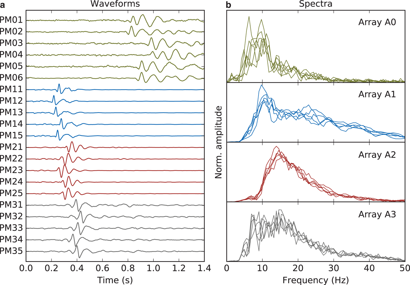
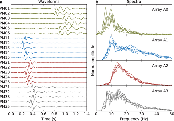
In this study, we use icequakes to investigate Rayleigh-wave azimuthal anisotropy. Rayleigh waves travel along the surface of a medium as a superposition of P-waves and vertically polarized S-waves. The resulting particle motion in a homogeneous, isotropic medium is confined to the plane spanned by the wave propagation direction and the vertical. In the presence of a velocity gradient in the subsurface, Rayleigh waves are dispersive, that is, their velocity is frequency dependent since the depth-penetration of Rayleigh waves is controlled by the wavelength. Inversion of the dispersion curve, therefore, allows the retrieval of subsurface parameters (e.g. Wathelet and others, Reference Wathelet, Jongmans and Ohrnberger2004). On glaciers, Rayleigh waves are produced by shallow ice cracking, which results in relatively small overtone/body wave arrivals. This allows for clear and unbiased surface wave dispersion measurements (e.g., Walter and others, Reference Walter2015). Since icequakes are abundant (hundreds to thousands per day, e.g. Roux and others, Reference Roux, Walter, Riesen, Sugiyama and Funk2010) and the vast majority of these events is of shallow type emitting dominant Rayleigh waves, they provide an effective passive source for the investigation of azimuthal anisotropy in crevasse fields. Figure 2a shows an example of such an icequake recorded by all 21 stations on Glacier de la Plaine Morte. For this study, we apply an array processing scheme to determine dispersion in each array, thus, our dispersion curves constrain ‘in situ’ average structure beneath each array. Azimuthal coverage of icequakes allows the study of azimuthal anisotropy and, since we are using Rayleigh waves, its variations with depth (Savage, Reference Savage1999). Surface crevasse icequakes produce signal in a broad frequency range (~10–50 Hz, Podolskiy and Walter, Reference Podolskiy and Walter2016). On Glacier de la Plaine Morte, we typically observe high signal levels between 10 and 30 Hz (Fig. 2b).
(a) Vertical-component waveforms of an icequake which occurred on 13 August 2016 and was recorded on all stations. Amplitudes are normalized. (b) Amplitude spectra associated with the waveforms shown in (a).
The first step of our processing is the detection and location of icequakes. Accurate location is crucial to later assign measured Rayleigh–wave dispersion at an array with the corresponding source back azimuth. In the following, we describe the beamforming technique which we use both to locate icequakes and to determine phase velocity dispersion curves. Subsequently, we briefly discuss azimuthal variations in Rayleigh wave phase velocities as introduced by Smith and Dahlen (Reference Smith and Dahlen1973).
Beamforming
Beamforming is a processing technique which uses the differential travel times of a seismic signal across an array of receivers to estimate its propagation direction (back azimuth) and slowness (inverse of velocity). The basic idea of beamforming is to shift the signals from all stations using a specific back azimuth-slowness combination and sum the traces. For a coherent signal, the traces will sum constructively if the true back azimuth and slowness are used (Rost and Thomas, Reference Rost and Thomas2002). For this study, we use a standard frequency-domain beamforming formulation which was previously used in several other studies (e.g. Gerstoft and Tanimoto, Reference Gerstoft and Tanimoto2007; Alvizuri and Tanimoto, Reference Alvizuri and Tanimoto2011; Diez and others, Reference Diez2016).
From the vertical ground motion recordings from N stations of an array, the Fourier transforms are computed at angular frequency ω and their (complex) values are arranged to form a column vector d(ω) of length N. Using this, the cross-spectral density matrix is computed as
 $$ \,{\bf C}(\omega) = \,{\bf d}(\omega) \,{\bf d}^{\dagger}(\omega),$$
where † denotes the complex conjugate transpose operation. Element C mn(ω) with  $m,\,n=1,\,\ldots ,\,N$ is the frequency-domain equivalent to the time-domain crosscorrelation of stations m and n, and yields the average phase delay at frequency ω between these two stations. Considering incident plane waves associated with slowness s and back azimuth Ψ, the modeled response for the same array at ω is given by
 $$\,{\tilde{\bf d}}(\omega,s,\Psi) = \exp \left(i \omega s \left(\bf\,{r} \cdot \bf\,{e}\right)\right),$$
where i is the imaginary unit, r is a N × 2 matrix containing the (x, y)-coordinates of the stations and e = (cos Ψ, sin Ψ)T (T is the transpose). Finally, the beam, or beam power, for a given frequency, slowness, and back azimuth is
 $$b(\omega, s, \Psi) =\, \mid\! \tilde{\bf {d}}^{\dagger}(\omega, s, \Psi) \,{\bf C}(\omega) \tilde{\bf d}(\omega, s, \Psi)\!\mid\!.$$
For calculating the beam, we take the norm of the cross-spectral density matrix and the modeled array response  $\tilde{\bf {d}}$. In this case, the beam power is normalized, that is, it is one in case the signal is coherent across the array and the true slowness and back azimuth are chosen and smaller otherwise. In order to stabilize the results, the beams from several successive discrete frequencies may be averaged (assuming that slowness and back azimuth are close to constant in the considered frequency band).
Azimuthal anisotropy
Weak seismic anisotropy can generally be described by a trigonometric polynomial of degree 4 in azimuth Ψ (Backus, Reference Backus1965). We follow Smith and Dahlen (Reference Smith and Dahlen1973) who derived a similar formulism for surface waves. In particular, they showed that the phase velocity of surface waves in an arbitrarily stratified and weakly anisotropic medium varies as
 $$\eqalign{c(\omega, \Psi) & = a_0(\omega) + a_1(\omega) \cos 2\Psi + a_2(\omega) \sin 2\Psi \cr & \quad + a_3(\omega) \cos 4\Psi + a_4(\omega) \sin 4\Psi,}$$
where the five coefficients a 0, a 1, a 2, a 3 and a 4 are dependent on the 21 independent elastic parameters of the elasticity tensor describing the anisotropic medium and are frequency-dependent integral functionals of depth. a 0 describes the ‘isotropic’, azimuthally averaged phase velocity, which can be different from the average phase velocity dispersion curve as determined in the next section, if azimuthal data coverage is insufficient. Forward modeling as well as observations suggest that Rayleigh wave azimuthal anisotropy in realistic physical media is dominated by 2Ψ variations (e.g., Smith and Dahlen, Reference Smith and Dahlen1973; Montagner and Nataf, Reference Montagner and Nataf1986; Montagner and Anderson, Reference Montagner and Anderson1989).
PROCESSING AND RESULTS
Icequake locations
Triangulation
To locate icequakes, we use the four arrays as ‘single summary’ stations to then triangulate to the icequake. For each array, we scan the continuous, bandpass filtered (10–20 Hz for arrays A1–A3; 7–15 Hz for array A0) data of all array stations using a classical short-term average/long-term average (STA/LTA) trigger (e.g. Allen, Reference Allen1978). As length for the STA and LTA windows, we use 150 samples (0.3 s for A0 stations and 0.375 s for A1, A2 and A3 stations) and 1800-sample windows (3.6 and 4.5 s), respectively, and set a trigger threshold for the STA/LTA ratio of 8. For the three seconds of data trailing a detected event, the trigger is disabled to avoid overlapping events. In order to consider a triggered signal an event, we require at least three stations to trigger concurrently. For each triggered event, we then automatically apply beamforming by averaging the beams obtained at discrete frequencies from 10 to 20 Hz (7 to 15 Hz for array A0 due to the larger aperture) in 0.2 Hz steps. We chose this frequency band since most shallow icequakes peak in amplitude in this range (Fig. 2b). We apply a grid search over back azimuth (in two-degree steps) and slowness. Since we are interested in Rayleigh waves, we use a coarse grid of slowness values associated with the minimum and maximum phase velocities of 1.25 and 2.25 km s−1, which covers the typical range expected for Rayleigh waves on glaciers (Walter and others, Reference Walter2015). As the final back azimuth and slowness, we chose the back azimuth-slowness combination which yields the maximum beam power. Figure 3a illustrates the results of this processing applied to the icequake shown in Fig. 2. To gain a robust result, we only use icequakes in our further analysis where the maximum beam power is larger than 0.75. This threshold effectively rejects events for which the plane wave assumption is violated or which exhibit a weak coherence across the array. In total, our processing scheme allows the detection of 71 113, 29 555, 9023 and 1052 events on arrays A0, A1, A2 and A3, respectively, of which 39 058, 28 134, 8791 and 977 events yield a beam power >0.75. The differences in events detected on different arrays indicate that many icequakes are too weak to be recorded on all arrays. In particular, array A3 encounters little seismicity compared with the other arrays (in terms of events per recording time unit).
(a) Beamforming applied to the icequake shown in Fig. 2. Shown is the beam power as a function of back azimuth (angular axis) and slowness (inverse of velocity, radial axis). The red dots indicate the maximum beam power. Its value (max) and the corresponding back azimuth (baz), slowness (slw) and phase velocity (vel) values are given in the centers of the polar plots. (b) Epicenter determination by triangulation for the icequake shown in Fig. 2. Shown are the back azimuths (colored cones) estimated for this icequake. The cone angle of ±1° accounts for the discrete grid search in 2° steps. The epicenter (black dot) is calculated as the average coordinates of all beam intersections and its error is estimated as the standard deviation thereof.
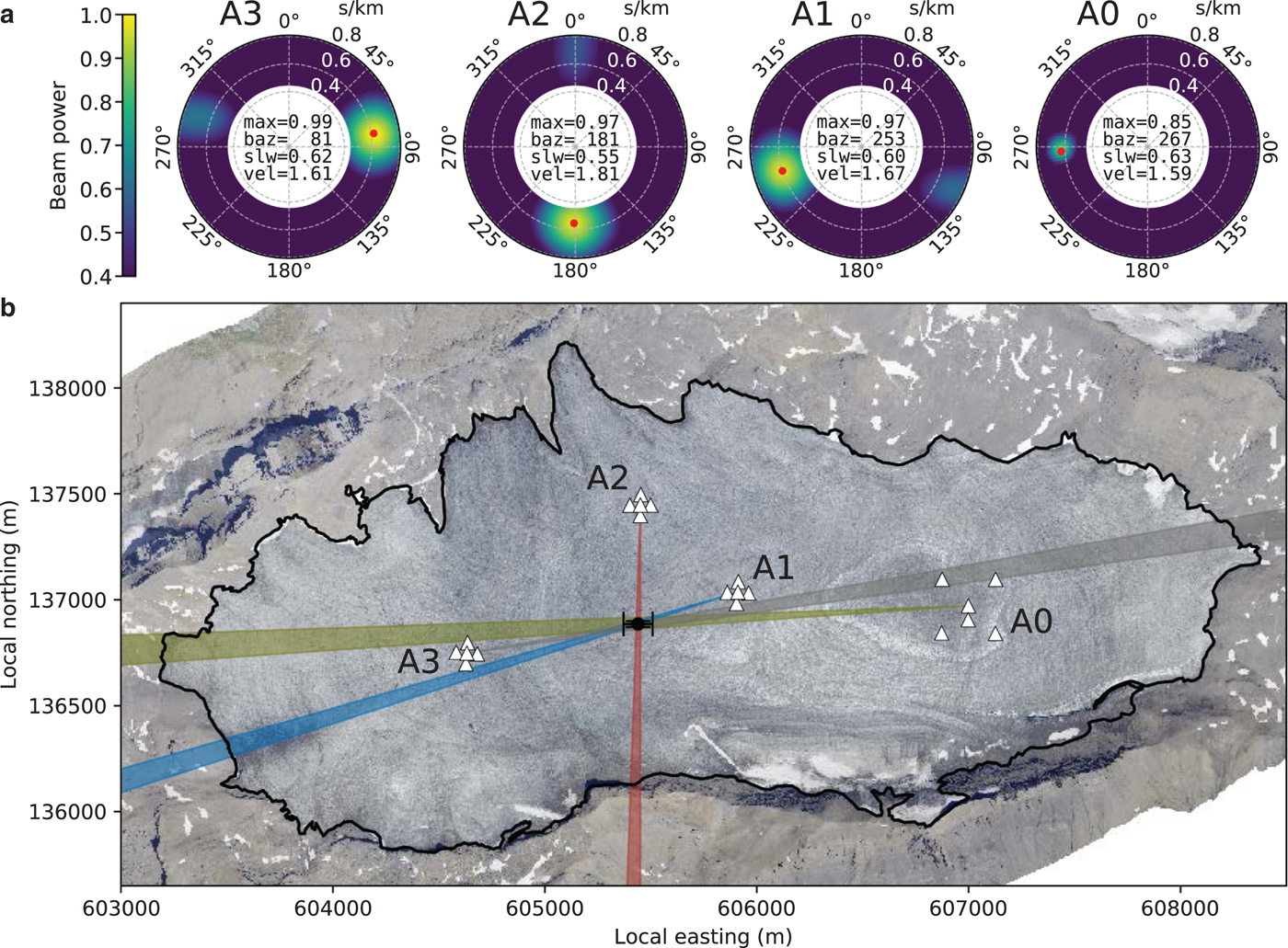
In the final step to triangulate to each icequake and thereby determine its location, we associate events triggered on different arrays. In case an event was triggered concurrently on different arrays (and accounting for the travel-time difference between different arrays), we use the back azimuth values determined in the previous step from these arrays and estimate the event epicenter by triangulation in the horizontal plane assuming a flat glacier surface. An example is shown in Fig. 3b for the icequake shown in Fig. 2. In 15 138 cases, we can associate the waveforms recorded concurrently on different arrays with the same event. However, since many icequakes were too small in magnitude to be detected on all arrays, we locate many icequakes using two, or three arrays, only. For those events which were detected on two arrays only (11 928 icequakes), we estimate the icequakes' epicenter as the point of intersection of two beams. In the case that three or four arrays detected an event concurrently (3210 icequakes), we determine its epicenter as the average of all beam pair intersections in x (East-West) and y-direction (North-South). Since accurate icequake locations are crucial for the investigation of azimuthal anisotropy (see also next section), we set the following thresholds for location uncertainty. For events located using two arrays, we require the angle of intersection of the beams to be in the range 90° ± 45°. For instance, we discard icequakes which were located by two arrays with similar back azimuth estimates since these locations are very sensitive to inaccuracies in the back azimuth measurements. In the most extreme case, two arrays might yield the same back azimuth which prohibits an epicenter determination. For events located using at least three arrays, we require the uncertainties in x- and y-direction to be smaller than 100 m. We estimate the uncertainties as the standard deviation of the beam-intersection points in x- and y-direction. Applying these criteria results in 9089 events for further analysis.
Secondary vetting of icequakes
From the 9089 events associated with the high-certainty location, we select only a subset for the investigation of azimuthal anisotropy. In particular, we only select events which fulfill the following conditions. First, we require the events to be at least 500 m away from the center of the considered array. This condition is necessary because we determine the phase velocity dispersion curves by plane-wave beamforming. Closer events would require a more complex wavefront, such as that of a spherical wave. In addition, such nearby events may be subject to near-field effects. For the lowest considered frequency of around 10 Hz and a Rayleigh wave velocity of 1.65 km s−1 (Walter and others, Reference Walter2015), the minimum distance of 500 m corresponds approximately to three times the maximum wavelength; a plane wave assumption is therefore reasonable. Second, from the events which pass this criterion, that is, are at least 500 m away from the array, we finally select only those which exhibit a dominant Rayleigh wave. By means of visual inspection, we discard all events which show strong body waves, unidentifiable phases, noisy records, or instrumental glitches. The latter was a frequent problem for records at array A3. We apply this selection procedure to the event data bases of arrays A1, A2 and A3, but not for array A0 and omit this array in the further analysis. The reasons are as follows: (i) due to the larger array aperture, array A0 has a different array response function compared with the other arrays (Fig. 3a). For the same reason, we encountered spatial aliasing for frequencies of 19 Hz and higher. Hence, the different array characteristics complicate the comparison of the arrays. (ii) Array A0 consists of borehole sensors whose azimuthal orientation is unknown. This implies that visual inspection of the particle motion in the Rayleigh polarization plane in order to identify Rayleigh phases (as done for arrays A1, A2 and A3) is not possible.
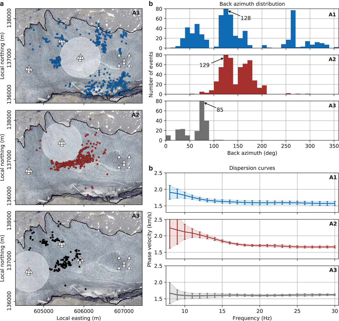
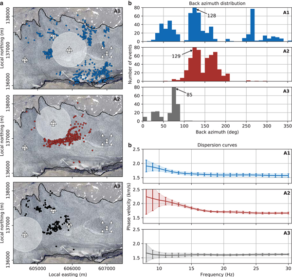
After the event vetting process, we are left with 1370 events of which 709, 570 and 211 events were recorded at arrays A1, A2 and A3, respectively. Their spatial and azimuthal distributions are shown in Figs 4a and 4b. Initially, many more events were available, however, we think that our restrictions are important to ensure robust azimuthal anisotropy results.
(a) Located icequakes selected for the investigation of azimuthal anisotropy at arrays A1 (blue), A2 (red) and A3 (black). The selected events are at least 500 m away from the array center (outside the white shaded area), their epicenters are associated with small uncertainties, and they exhibit a dominant Rayleigh wave (for details see text). (b) Azimuthal distribution of the icequakes shown in (a). The arrows with numbers indicate the height of the clipped bars. (c) Average Rayleigh wave dispersion curves (solid lines) calculated from the events shown in (a). The errorbars indicate one standard deviation.
Phase velocity measurements
Our last processing step involves the calculation of the Rayleigh wave dispersion curves. For each array and event shown in Fig. 4a, we cut a narrow window containing the Rayleigh waves of all array stations and apply plane-wave beamforming. For each event, we fix the back azimuth to the value determined previously and perform a fine grid search on phase velocities only (1–4 km s−1 in 0.005 km s−1 steps). In the initial beamforming step to locate the icequakes, we kept the slowness grid intentionally coarse in order to save computation time. For the same reason, we determined a single phase velocity value for the frequency range 10–20 Hz (7–15 Hz for array A0), only. By contrast, we now determine the phase velocity as a function of frequency, in 1 Hz steps, to obtain a dispersion curve instead of a single value. In order to obtain a smooth dispersion curve, we use a 4 Hz wide sliding window with 75% overlap resulting in phase velocity measurements at all integer frequencies from 8 to 30 Hz. Within the sliding window, we average the beams obtained at discrete frequencies in 0.2 Hz steps and associate the slowness value which maximizes the beam power with the center frequency of the 4 Hz wide window.
Overall, the final dispersion curves at each array are consistent and cluster within a few percent around the average dispersion curves, as shown in Fig. 4c. With phase velocities between ~2.2 km s−1 at 8 Hz (array A2) and 1.6 km s−1 at 30 Hz (all arrays), the dispersion curves are similar to curves observed previously on glaciers (e.g., Walter and others, Reference Walter2015). A decrease in phase velocity with increasing frequency is consistent with a seismically slower medium (such as glacial ice) over a faster bedrock medium. At low frequencies, phase velocities are lowest at array A3 which has the thickest ice cover, and highest at A2 which has the thinnest ice cover. All these observations are consistent with a two-layer ice/bedrock model that shows lateral variations as described. Note here, however, that the average dispersion is the statistical average of our measurements. In the presence of lateral heterogeneity and/or azimuthal anisotropy, this average does not necessarily reflect the true average, isotropic phase velocity a 0 in Eqn 4.
Azimuthal anisotropy
It becomes apparent, that the azimuthal distribution of the events is different for each array (Fig. 4b). Array A1 exhibits the best azimuthal distribution of events, followed by A2 which has many events distributed in the back azimuth range of 90–210°, thus populating a range well above a quadrant. By contrast, A3 has a poor azimuthal distribution. Since the majority of events is found at azimuths between 60° and 90°, the data coverage does not justify further in-depth study of azimuthal anisotropy. We, therefore, focus on arrays A1 and A2 in the following.
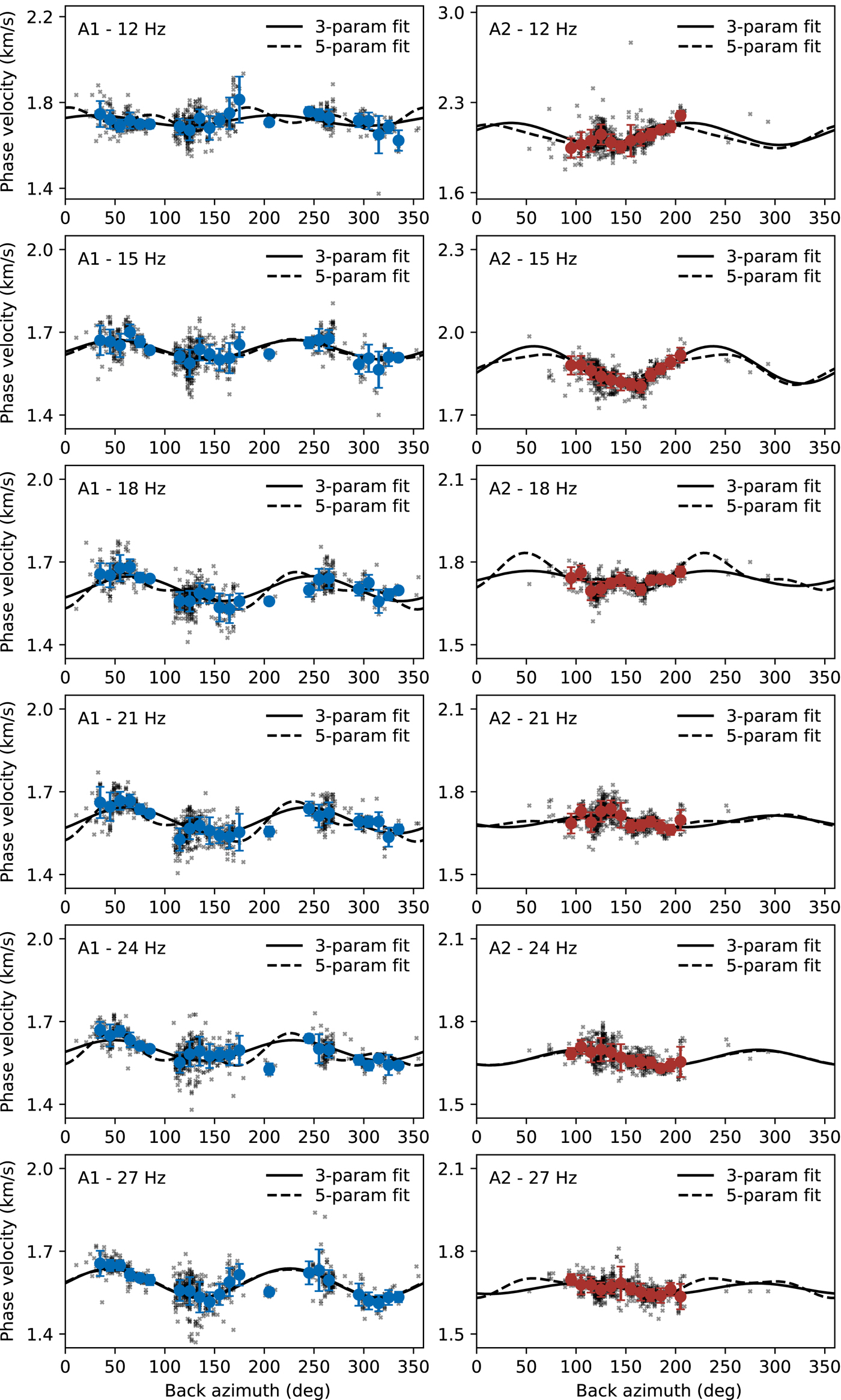
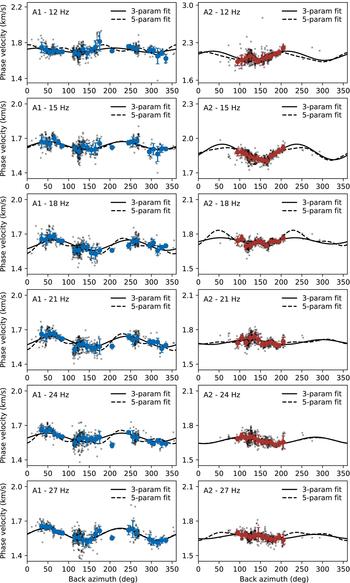
To investigate azimuthal anisotropy, at each frequency considered, we sort the measured phase velocities as a function of back azimuth Ψ. To smooth the data somewhat, we calculate the average phase velocity and its standard deviation in 10° bins where at least six measurements are available. Through these data points, we perform least-squares fits to obtain the coefficients a 0, a 1, a 2, a 3, a 4 in Eqn 4. We do not weight the data with their errors. As stated earlier, Rayleigh wave azimuthal anisotropy is dominated by 2Ψ variations (e.g., Smith and Dahlen, Reference Smith and Dahlen1973; Montagner and Nataf, Reference Montagner and Nataf1986; Montagner and Anderson, Reference Montagner and Anderson1989). We adopt this idea and perform a least-squares fit for a 0, a 1 and a 2 only to determine the final azimuthal anisotropy. Though, a fit for all 5 coefficients is an useful consistency check, as a 3 and a 4 should be negligible. We then assign the difference between the two fits as error bars to our final results. Figure 5 summarizes the results of the least-squares fits for arrays A1 and A2 at six discrete frequencies. The least-squares fits after Smith and Dahlen (Reference Smith and Dahlen1973) for all integer frequencies are shown in Figs S1 and S2 in the supplementary material.
Phase velocity measurements as a function of back azimuth for array A1 (left column, blue) and array A2 (right column, red). Gray crosses are the measurements from single icequakes, blue and red dots are bin averaged values in 10° bins containing at least six measurements (error bars are one standard deviation). The dashed line is the five-parameter model fit after Smith and Dahlen (Reference Smith and Dahlen1973) (Eqn 4) through the bin-averaged values. The solid line is the three-parameter fit omitting the 4Ψ terms.
Array A1
For array A1, the phase velocities at 12 Hz scatter and a systematic pattern is not discernible (Fig. 5). Consequently, the resulting fits for 3 and 5 coefficients lead to different predictions (solid and dashed lines). At 15 and 27 Hz, the three-parameter fit and the five-parameter fit lead to almost identical predictions, implying that the 4Ψ terms are small. For the intermediate frequencies (18, 21, 24 Hz), the five-parameter fit shows moderate deviation from the three-parameter fit (peak-to-peak amplitude of the 4Ψ contribution, that is,  $2 \sqrt {a_3^2 + a_4^2}$, is 42, 50, 46 m s−1, respectively). In the next step, we log the strength of anisotropy and the fast direction, very much in analogy to determine anisotropy-induced shear-wave splitting (Savage, Reference Savage1999) parameters. The determined strength of the frequency-dependent azimuthal anisotropy is the peak-to-peak amplitude of the 2Ψ variation divided by the estimated isotropic phase velocity a 0, that is, $2\sqrt {a_1^2 + a_2^2}/a_0$. The error is estimated as the difference between the peak-to-peak amplitude of the three-parameter fit and the peak-to-peak amplitude of the five-parameter fit divided by the isotropic phase velocity. As the second anisotropy parameter, we quantify the fast direction as the peak of the three-parameter fit (in the 0°–180° range) and its error as the deviation of the peaks of the three-parameter fit to the five-parameter fit.
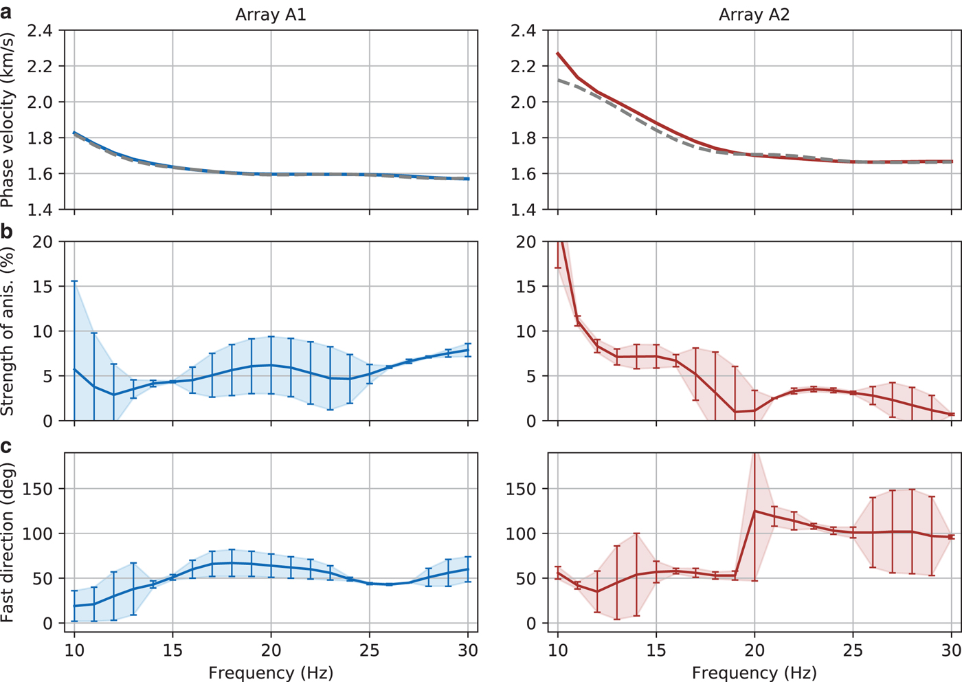
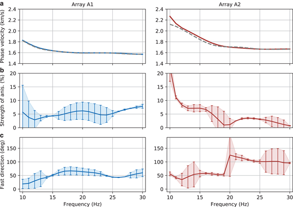
The results are shown in Figs 6b and 6c. As discussed earlier, scatter in the data is considerable for low frequencies and an anisotropy pattern does not emerge. For frequencies of 14 Hz and higher, azimuthal anisotropy is present and its strength increases from ~4% at 14 Hz to ~8% at 30 Hz, although results at intermediate frequencies (17–24 Hz) have large error bars (Fig. 6b). The fast direction changes somewhat with frequency but largely stays around 55° (Fig. 6c).
(a) Isotropic phase velocities (a 0 parameters from three-parameter fits) for array A1 (blue) and array A2 (red). The gray dashed line is the average dispersion curve obtained from beamforming shown in Fig. 4c. (b) Strength of anisotropy, that is, peak-to-peak amplitude of the three-parameter fit divided by the isotropic velocity in percent. (c) Fast direction of wave propagation determined as the maximum of the three-parameter fit in the 0° to 180° degree range. The errorbars in (b) and (c) are estimated from the deviation of the three-parameter and the five-parameter fit (see text for details).
Array A2
Azimuthal anisotropy at this array is assessed in the same way as for array A1. From Figs 5 and S2, we see that even though scatter in the phase velocity measurements is considerable, there is evidence for azimuthal anisotropy at low frequencies. At frequencies of ~15 Hz our data reveals azimuthal anisotropy with a strength of ~7% and a fast direction of ~55° (Figs 6b and 6c). At higher frequencies, azimuthal anisotropy is barely discernible. To summarize, we find azimuthal anisotropy for low frequencies (~15 Hz) but not at higher frequencies. This is indicative of an anisotropic layer at depth, and not near the top.
MODELING OF DISPERSION CURVES
Basic forward modeling and inversions described in the following allow a rough first-order estimate on the underlying ice properties with depth. For this purpose, we use the Geopsy package (geopsy.org; Wathelet and others, Reference Wathelet, Jongmans, Ohrnberger and Bonnefoy-Claudet2008). We use a two-track approach where we perform forward modeling to explore specific targets in the model space (e.g. layer thickness) but also apply a more modern approach involving a formal inversion. We start with the forward modeling because we want to gain improved insight into which parts of the model are better constrained than others, and which parts resulting from the inversion may not be required to fit the data. Another reason why we follow both tracks has to do with the sensitivity of Rayleigh wave phase velocity to structure with depth. Rayleigh waves are sensitive to both shear and compressional wave velocity, Vs and Vp, as well as density (Fig. 7). Of the three, sensitivity to Vs is greatest, but sensitivity to shallow Vp and density can be significant. Note that sensitivity to Vp is typically enhanced where sensitivity to Vs is decreased. Sensitivity to Vp and density is often ignored and inversions are performed only for Vs in order to keep an inversion well-conditioned. In our tomographic inversions for deeper Earth structure, we prefer to account for sensitivity to Vp and density by scaling the respective kernels to that of Vs, using known scaling relationships for Earth materials, and then perform inversions for Vs. To assess the impact of ignoring sensitivity to Vp and density, we scale the kernels during forward modeling but keep Vp and density fixed to a starting model in the inversions.
Sensitivity kernels for Rayleigh wave phase velocity at 10 and 30 Hz as suitable for modeling at array A1. The underlying two-layer model consists of 100 m of ice over a half-space of karstic bedrock. The parameters for this model are summarized in Table 1. The kernels were computed using the MATLAB code of Haney and Tsai (Reference Haney and Tsai2017).

Gorner-karst (GK) model used as the starting model in this study

Our starting model uses the values of Walter and others (Reference Walter2009), found for the Gorner Glacier at the nearby Monte Rosa Massif. For the basement, we use typical limestone values reported by Assefa and others (Reference Assefa, McCann and Sothcott2003), since the geology beneath Glacier de la Plaine Morte is characterized by a karst environment formed by this rock type (Finger and others, Reference Finger2013). Table 1 summarizes the model, which we subsequently call the Gorner-Karst (GK) model.
At array A1, we fix the ice-basement boundary at 100 m. The sensitivity kernels computed for this array (Fig. 7) indicate that phase velocities in the frequency range considered here (10–30 Hz) are most sensitive to the structure at a depth <100 m, with only frequencies near 10 Hz or less having a rather low sensitivity to Vs below the ice-basement boundary. Because sensitivity is high just above the boundary, our dataset is actually sensitive to the depth of the boundary. To stress this point, kernels computed for an ice thickness of 70 m, as assumed for A2 (Fig. S3), confirm that our data can indeed depend on structural changes well below a depth of 100 m. Sensitivity to these depths may be suppressed as error bars increase with decreasing frequency (Figs 4c and 6).
A first step is to model the average phase velocities at arrays A1 and A2 (Fig. 6a). We seek the simplest two-layer ice-basement model that fits the data reasonably well. Targeted forward modeling for array A1 confirms that an interface near 100 m explains a slow increase in phase velocity with declining frequency below 15 Hz (Fig. S4). The shear wave velocity in the ice has to be 4% less than in the GK model to match phase velocities at high frequencies. We cannot find a simple 2-layer model that fits phase velocities at frequencies below 13 Hz. A 3-layer model with two ice layers, where the bottom 30 m have 5% higher values than in the ice layer above slightly improves the fit to the data between 10 and 13 Hz. Our data are not sensitive to small changes (8% or less) in basement Vs and Vp. However, a deeper interface near 120 m, as suggested as a deeper limit by the helicopter-borne GPR data, is inconsistent with our observations. This is confirmed by both targeted forward modeling as well as inversions. For array A2, a shallower interface near 70 m or slightly shallower is needed to explain the increase starting at 20 Hz (Fig. S5), and ice parameters are elevated by 1% compared with the GK model. For both A1 and A2, inversions in which the interface is a free parameter (for details on the inversions see next section) tend to return slightly shallower interfaces (90 and 60 m, respectively).
MODELING OF AZIMUTHAL ANISOTROPY
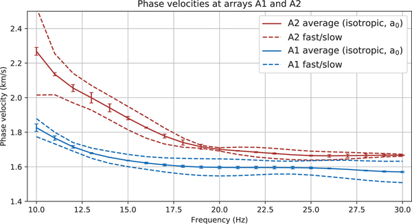
In anisotropic media, the wave speed changes with direction. In transversely isotropic media with vertical symmetry axis, the description of compressional and shear wave velocities, Vp and Vs separate into vertical and horizontal velocities, that is, Vpv, Vph, Vsv and Vsh. Here, the sensitivity of Rayleigh wave phase velocity to Vsv and density is essentially the same as in the isotropic case while sensitivity to Vsh is negligible. Sensitivity to Vp is increased at depth compared with the isotropic case but still much smaller than the sensitivity to Vs. Montagner and Nataf (Reference Montagner and Nataf1986) discuss such depth sensitivities to derive anisotropy as a function of depth. In the conceptually simplest case, Rayleigh wave azimuthal anisotropy occurs when a transversely isotropic medium is tilted. Assuming that the fast and slow phase velocities can be modeled independently, the resulting Vs models allow an initial assessment of the degree of anisotropy with depth. This assumption may not be valid for media with general anisotropy, but our approach may be an acceptable starting point, particularly for media whose main symmetry axis is horizontal. For the purpose of exploring the model space, and possible inconsistencies, we follow two different strategies in the forward modeling and in the inversions. For the latter, we attempt to fit the fast and slow dispersion curves shown in Fig. 8 independently and estimate anisotropy from the resulting Vs models. In the forward modeling, we try to fit both average phase velocities and strength of anisotropy as displayed in Fig. 6 by varying the shear wave velocity and the thickness of the anisotropic layer.
Average (isotropic) phase velocities (solid lines with error bars) and fast and slow phase velocities (dashed lines) as obtained from the 2Ψ-coefficients. The error bars of the average dispersion curve represent the difference of the a 0 coefficients between the three-parameter fit and the five-parameter fit.

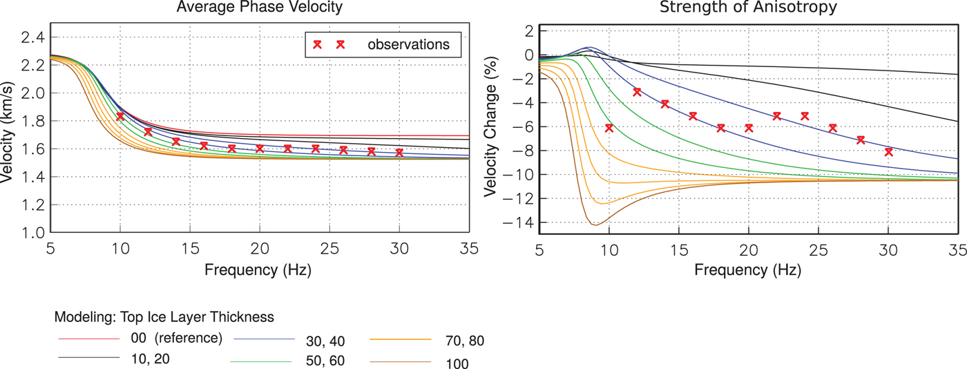
At array A1, the degree of azimuthal anisotropy increases with frequency, providing evidence for a shallow anisotropic layer rather than a deep one. We use the GK model as starting model to predict the average dispersion and mimic anisotropy by allowing an upper ice layer with reduced velocities. During iterative, targeted forward modeling, we vary Vs in the ice as well as the thickness and strength of anisotropy in the top ice layer (Fig. 9). In the final set of runs, Vs in the lower ice layer was set to 3% higher than in the GK model. The top ice layer had the same Vs in the fast direction and 10% reduced Vs in the slow direction (hence the negative velocity change in the right panel). We conclude that a 30–40 m thick upper ice layer with 10% Vs anisotropy explains both the frequency-dependent average phase velocity as well as the strength of anisotropy. The thickness of the top layer trades off with the degree of anisotropy in such a way that a 20–30 m thick layer with 15% anisotropy is also consistent with our data.
Results from the final set of targeted forward modeling at array A1. The underlying model has two ice layers with an isotropic lower layer, and an anisotropic upper layer with varying thickness (marked by different colors) and 10% anisotropy. The total ice thickness was fixed at 100 m. See text for details.
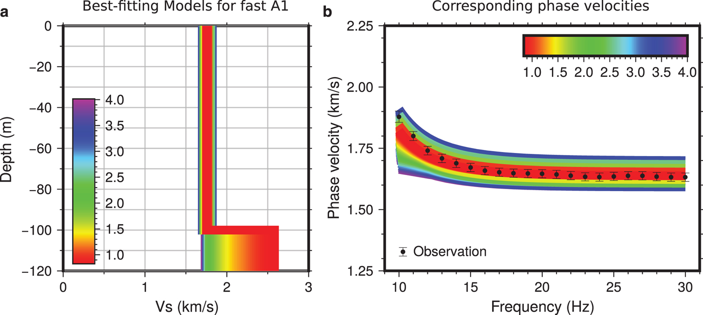
For formal inversions, we use the Dinver tool included in the Geopsy package. The embedded neighborhood algorithm (Sambridge, Reference Sambridge1999a,Reference Sambridgeb) allows the estimation of model uncertainties. To balance out the weight of the data in the inversions and to avoid the dominance of data with perhaps unrealistically small error bars, we set the minimum error threshold to 1%. We first seek a model with one ice layer that fits the fast phase velocity (Fig. 10). We then use this model as the starting model to fit the slow phase velocity but now allowing a second ice layer on top, with varying Vs and thickness. The resulting best-fitting models are summarized in Fig. 11 and Table 2. As noted in the section on forward modeling, basement Vs is not well constrained by our data but the best-fitting model has a basement Vs of 2582 m s−1 (3% higher than in the GK model). Raising the basement Vp to 4500 m s−1 as in the GK model leads to higher Vs (2711 m s−1) where the Vp/Vs ratio of 1.8 as typically found for limestone (Assefa and others, Reference Assefa, McCann and Sothcott2003) is no longer preserved. We stress once again that basement velocities at A1 are not well constrained. Shear wave velocities in the lower ice layer cluster around our best-fitting value of 1752 m s−1. As far as the top, anisotropic ice layer is concerned, the best-fitting model has a 40-m-thick ice layer with 7.8% anisotropy in Vs. A slightly thinner, more anisotropic layer fits our data nearly equally well. This is in agreement with results from our targeted forward modeling.
(a) Best-fitting models for the fast phase velocities at array A1. (b) Corresponding predictions, different colors denote the misfit. Well-fitting models should have a misfit near 1 or less.
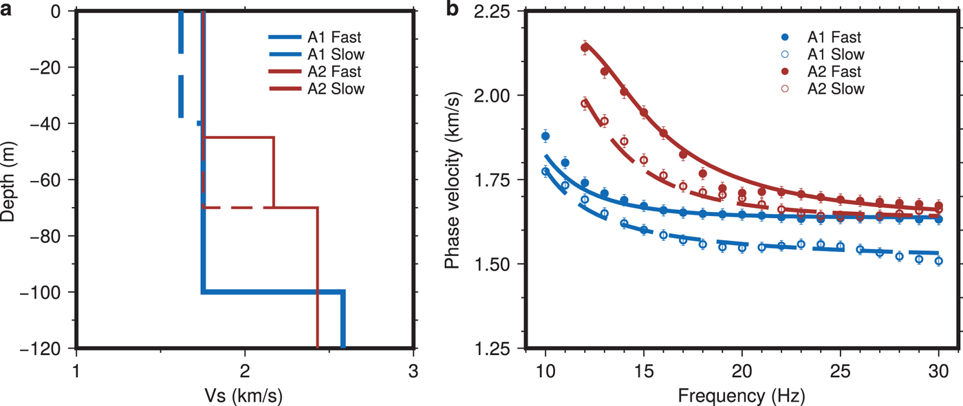
(a) Summary plot showing both the fast (solid line) and slow (dashed line) Vs models at arrays A1 (blue) and A2 (red). (b) Data (circles) and model predictions (solid and dashed lines) for the Vs models on the left.
Best-fitting models for Array A1
The situation at array A2 is different as azimuthal anisotropy is very weak at high frequencies but increases in strength with decreasing frequency (Figs 6b and 8). This is indicative of a deep anisotropic layer. Also, note that phase velocities at high frequencies match those for the fast velocities at array A1. This means that upper ice velocities likely match those at A1. In the inversion, we start with the fast A1 Vs model as slow Vs model at A2. We keep the ice thickness fixed at 70 m. After inversions, results for basement Vs cluster around 2430 m s−1 and so are slightly lower than at A1 (Table 3). Repeat inversions using 4500 m s−1 as Vp yields the same Vs, so it seems that basement Vs is well-constrained at A2. For modeling anisotropy, we allow a lower, faster ice layer to vary in Vs and thickness. The best-fitting model has a 25-m-thick lower ice layer with 23.8% anisotropy in Vs (Table 3). Realizing that this inversion yields perhaps unrealistically high Vs for the ice, we explore other options through targeted forward modeling. We notice that phase velocity undulates somewhat around an ‘average’ trend as frequency increases, with a slight dip between 17 and 21 Hz (Figs 6a and 8). We suspect internal data inconsistency because no simple 2-layer ice-basement model appears to be able to fit the data between 12 and 14 Hz and above 21 Hz on one hand and those between 15 and 20 Hz on the other equally well. Forward modeling yields a 20–30 m thick anisotropic layer at the bottom of the ice where the slow phase velocities can be matched quite well with the GK model. The fast phase velocities require a Vs in the bottom layer that is at least 10% higher. At 1936 m s−1, this higher Vs remains well below the Vs obtained in the inversion (see case 1 in Fig. S6). A thinner, 20 m layer requires a higher Vs of 2024 m s−1 in the lower ice layer or a higher basement Vs of 2625 m s−1. The elevated basement Vs has no impact on the fit to the slow phase velocities and is still a reasonable value found for limestone (Assefa and others, Reference Assefa, McCann and Sothcott2003). The option of the higher basement Vs (by 8% compared with that in Table 3) is not found in the formal inversion, possibly as a result of the internal inconsistency of the data.
Best-fitting models for Array A2
SURFACE CREVASSE DETECTION FROM IMAGERY
Forward modeling and inversion of dispersion curves reveal, that the observed anisotropy beneath array A1 is associated with the shallow ice. To test our hypothesis of crevasse-induced anisotropy, we determine the surface strike of the crevasses (direction parallel to the crevasses) at the A1 field site and compare the result with the observed fast direction of wave propagation.
To obtain the orientation of the crevasses, we apply the Canny edge detector (Canny, Reference Canny1986) to orthophotographs (by swisstopo, SWISSIMAGE) of the glacier surface taken in 2015. Because the ice flow of Glacier de la Plaine Morte is negligible, we do not expect a change in crevasse pattern from the time of image acquisition in 2015 to our field campaign in 2016. Orthophotographs from 2016 are not usable because the snow cover did not vanish completely. Nevertheless, comparison of 2015 and 2016 images confirm that major features stay unmodified. We choose a 200 m × 200 m snippet from the 2015 images centered on the central station of array A1 (Fig. 12a) and load it as grayscale image preserving the intensity information. First, we smooth the image using a two-dimensional Gaussian filter with a standard deviation of the Gaussian kernel of 3 in both directions. Second, we calculate the intensity gradients Gx and Gy of the image in x- (Fig. 12b) and y-direction (Fig. 12c) using Sobel kernels (e.g. Jähne and others, Reference Jähne, Haussecker and Geissler1999). Since the crevasses on the orthophotograph appear as dark lines on the otherwise bright ice, the differentiation with respect to intensity reveals the crevasses as shown in Figs 12a–c. Ultimately, the orientation (or back azimuth) of the crevasses is obtained by the arctangent of the intensity-derivative ratio calculated for each pixel, that is, tan Ψk = G y,k/G x,k for the k-th pixel.
Orientation of surface crevasses. (a) 200 m × 200 m orthophotograph of the glacier surface surrounding array A1 (white triangles). Some but not all crevasses are highlighted by arrows. Easting and Northing (in Swiss Grid coordinates) of the lower left corner are 605811 m and 136936 m, respectively. (b) Intensity-derivative in x-direction of a grayscale image version of (a) using Sobel kernels. (c) Same as (b) in y-direction. (d) Orientation (back azimuth) of surface structures evaluated for each pixel from intensity ratios of image in (c) and (b) (black histogram; see text for details). The blue curve is the frequency-averaged azimuthal anisotropy at array A1 for the frequency range 14–30 Hz.
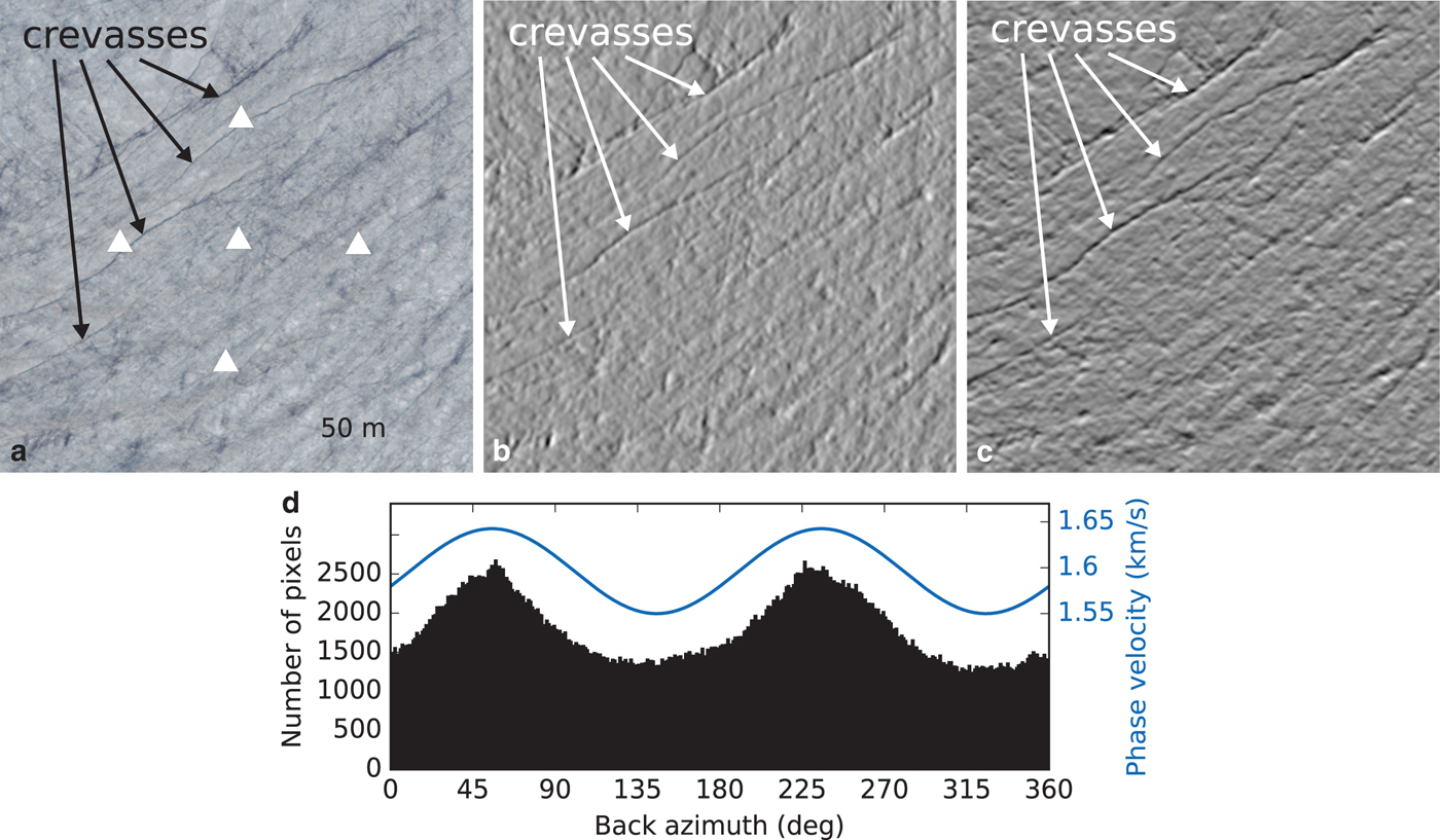
As can be seen from Figs. 12b and 12c, the crevasses are the dominant features detected by calculating the intensity gradients. In addition, a histogram calculated from all pixel orientations (Fig. 12d) yields a dominant orientation of approximately 55° (and 235°, i.e. 55° + 180°), which is in agreement with the surface strike of the crevasses as determined by visual inspection. Furthermore, comparing this with the average anisotropy fits in the frequency range 14–30 Hz (the frequency range where observed anisotropy is strongest; Fig. 6), we find that the Rayleigh waves propagate fastest in the direction of the crevasse surface strike (Fig. 12d).
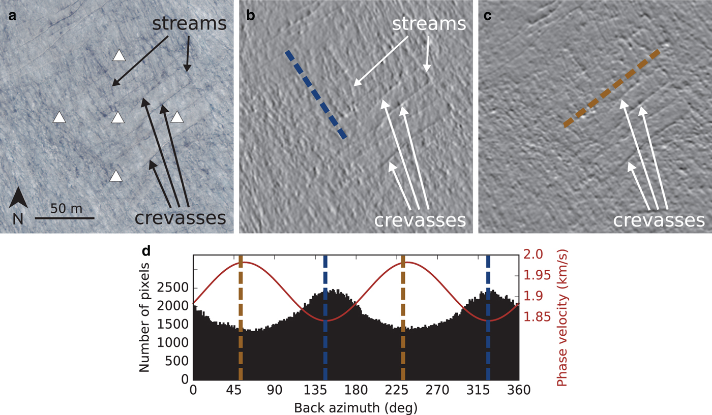
At field site A2, azimuthal anisotropy is found at depth, and we should not expect to find that surface crevasses can explain our observations. Nevertheless, we find that the fast direction of wave propagation for low frequencies is parallel to the surface crevasses. This is shown in Fig. 13d by comparing the fast direction to the surface strike of the narrow crevasses as determined by means of visual inspection (brown dashed line in Figs. 13c and 13d). In this case, our image processing does not pick up the crevasses as dominant features. Reasons for this are (i) the crevasses at this field site are narrower (centimeter to decimeter scale) compared with array A1 and (ii) several supraglacial streams following the approximate topographic gradient are present. Consistent with visual inspection, the image processing yields the dominant direction of these supraglacial streams (blue dashed line in Figs. 13b and 13d). Even though the streams are surficial, water might also flow englacially in the shallow (~2 m), porous weathering crust (Irvine-Fynn and others, Reference Irvine-Fynn, Hodson, Moorman, Vatne and Hubbard2011; Cook and others, Reference Cook, Hodson and Irvine-Fynn2016). Since the water flow is in a preferred direction, structural anisotropy might be present in this layer. However, the weathering crust is formed by solar radiative heating (Fountain and Walder, Reference Fountain and Walder1998), thereby forming in a planar fashion, allowing the water to also distribute laterally away from the streams. Additionally, meltwater also penetrates the weathering crust directly where it is produced without draining in a supraglacial river. For this reason and due to the thinness of this layer, we do not expect that the weathering crust introduces strong anisotropy for seismic wave propagation.
Same as Fig. 12 but for array A2. (a) Easting and Northing (in Swiss Grid coordinates) of the lower left corner are 605351 m and 137346 m, respectively. In (b) and (c), the approximate surface strike of supraglacial meltwater streams and crevasses are indicated by the dashed blue and brown lines, respectively. The back azimuth of these lines are also shown in (d). The red line in (d) shows the average azimuthal anisotropy found in the frequency range 12–16 Hz. Note that our image processing picks up the orientation of the streams and not the orientation of the crevasses.
DISCUSSION
In the case of crevasse-induced azimuthal anisotropy, we expect that the fast direction of Rayleigh-wave propagation is parallel to the crevasse alignment (Crampin, Reference Crampin1978). For array A1, we showed that such a correlation exists. Comparison of the fast direction at high frequencies (14–30 Hz) with the surface strike of crevasses (Fig. 12d) revealed that Rayleigh waves travel the fastest parallel to the crevasses. In addition, the estimated thickness of the crevassed, anisotropic layer of 30–40 m is within the theoretical and observed penetration depths of crevasses (Van Der Veen, Reference Van Der Veen1998). Even though a maximum penetration depth of ~30 m is often stated for air-filled crevasses (e.g. Irvine-Fynn and others, Reference Irvine-Fynn, Hodson, Moorman, Vatne and Hubbard2011), deeper crevasses of this type have been reported (Colgan and others, Reference Colgan2016, and references therein). In the presence of water, crevasses can penetrate even substantially deeper (Van Der Veen, Reference Van Der Veen1998).
Apart from preferentially aligned crevasses, crystal orientation fabric (COF) can introduce seismic anisotropy in glacial ice (e.g. Diez and others, Reference Diez2014). In particular, a (thick) girdle fabric which is characterized by c-axis orientations of the single ice crystals in a vertical plane but with various angles relative to the horizontal represents a transversely isotropic medium with horizontal symmetry axis exhibiting azimuthal anisotropy (Diez and Eisen, Reference Diez and Eisen2015). Vs, and thus the most sensitive parameter for Rayleigh waves, can vary by more than 10% in such a medium (Maurel and others, Reference Maurel, Lund and Montagnat2015). However, in most (alpine) valley glaciers and on another plateau glacier in the same mountain range, multiple-maximum fabrics which contradict azimuthal anisotropy are found (Tison and Hubbard, Reference Tison and Hubbard2000; Hudleston, Reference Hudleston2015). For this reason – and given the correlation of fast direction with crevasse surface strike together with a reasonable thickness of the anisotropic layer – we interpret the observed azimuthal anisotropy beneath array A1 as crevasse-induced.
Compared with other cases of crack-induced anisotropy, the observed strength of up to 8% is an intermediate value. Bradford and others (Reference Bradford, Nichols, Harper and Meierbachtol2013) report only slightly more than 3% variation in p-wave velocity due to basal crevasses and Crampin (Reference Crampin1994) reports 1.5–4.5% shear-wave velocity anisotropy due to cracks in the Earth's crust. For heavily cracked rocks close to the Earth's surface, 10% or more are found (Crampin, Reference Crampin1994). Two observations of anisotropy caused by crystal fabric orientation in glacial ice cover the range 3–5% shear-wave velocity (Picotti and others, Reference Picotti, Vuan, Carcione, Horgan and Anandakrishnan2015; Smith and others, Reference Smith2017). Note, however, that these values are associated with shear-wave splitting in contrast to azimuthal variations of Vsv as reported in this study. Incorporation of Vsh-velocity measurements would allow us to study shear-wave splitting and thus crack density (Hudson, Reference Hudson1981; Crampin, Reference Crampin1981) but this is beyond the scope of this work.
In contrast to array A1, inversions for array A2 suggest that azimuthal anisotropy can be best explained by a 25-m-thick anisotropic layer at the base of the glacier with a shear velocity of 2170 m s−1 along the fast direction (Table 3). Targeted forward modeling revealed that the shear velocity in the lower ice layer trades off with its thickness as well as the basement velocity. Allowing a thicker ice layer or a higher basement velocity keeps the velocity in the lower ice layer below 2000 m s−1. In the region of array A2, ice flow, even though small (smaller than 1 cm d−1 as measured during the field campaign), might provide stresses for ice crystal alignment (Cuffey and Paterson, Reference Cuffey and Paterson2010). However, recrystallization in temperate ice often counteracts the formation of COF favorable for azimuthal anisotropy (Cuffey and Paterson, Reference Cuffey and Paterson2010; Hudleston, Reference Hudleston2015). In addition, even for a single ice crystal, neither the broad Vs-range from 1750 m s−1 to 2200 m s−1, nor the high Vs of 2200 m s−1 as suggested by our inversions can be explained (Maurel and others, Reference Maurel, Lund and Montagnat2015). By contrast, slower shear velocities of 1950 m s−1 as found by our forward modeling seem more consistent with predictions for temperate ice with preferred ice crystal alignment (Kohnen, Reference Kohnen1974; Diez and Eisen, Reference Diez and Eisen2015). Basal crevasses as found on Bench Glacier (Bradford and others, Reference Bradford, Nichols, Harper and Meierbachtol2013), would require a low-velocity layer and can therefore not explain our inversion and modeling results.
Because of the aforementioned issues in data coverage and quality, we are hesitant to draw definitive conclusions on the cause of the azimuthal anisotropy at array A2. In particular, insufficient coverage of icequakes may lead to overfitting of the data set (e.g. Burnham and Anderson, Reference Burnham and Anderson2003). Additionally, our forward modeling and inversion approach of slow and fast dispersion curves might not be well-suited for this array since (i) (in contrast to array A1) only a narrow frequency band (around 15 Hz) shows clear azimuthal anisotropy and (ii) azimuthal data coverage is incomplete. Another issue at this array is the observation of surface crevasses which do not seem to induce azimuthal anisotropy at high frequencies. We, therefore, speculate that these surface cracks might be either too shallow or too narrow and sparse in order to result in measurable azimuthal anisotropy of the high-frequency Rayleigh waves. Another explanation would be that the infiltration of water into the ice along the surface streams results in a shallow anisotropic layer. In turn, since the streams strike approximately perpendicular to the crevasses, azimuthal anisotropy associated with this layer could potentially cancel the crevasses' signature at high frequencies.
At this point, it remains unclear why the measured dispersion curves at arrays A1 and A2 both suggest a thinner glacier compared with the helicopter-borne GPR survey. Regarding the latter, ice thickness values beneath the arrays are obtained by an interpolation of the values along the flight profiles. Inaccuracies introduced thereby, which are expected bigger for A1 than for A2 due to coarser data coverage, explain some though unlikely all of the disagreement. Additionally, errors in the ice thickness estimates from dispersion curve inversions might arise from 3-D-topography effects at the ice/bedrock interface which our horizontally-stratified model does not account for.
SUMMARY AND CONCLUSION
In this study, we used naturally occurring icequakes to investigate azimuthal anisotropy of Rayleigh waves on Glacier de la Plaine Morte, Switzerland. In a first step, we automated the task of locating icequakes using beamforming and triangulation from up to four arrays. Using the located events, we then examined the phase velocity of Rayleigh waves as a function of back azimuth of wave propagation and frequency. For array A1, we find azimuthal anisotropy for high frequencies (~15–30 Hz) and, by means of forward modeling as well as inversion of dispersion curves, we showed that the corresponding depth range is the shallow ice (upper 40 m). Furthermore, by analysis of the surface strike of crevasses, we conclude that the observed anisotropy is caused by the preferential alignment of (near to vertical) surface crevasses. For array A2, we find evidence for azimuthal anisotropy at low frequencies, which most likely is caused by an anisotropic ice layer at the base of the glacier. Even though we are less confident in the results of this array due to poorer data quality and azimuthal distribution of icequakes compared with array A1, we argue that COF could be the cause for azimuthal anisotropy at this field site. Observed surface crevasses at array A2, though narrower compared with those at the array A1 and potentially less deep, do not seem to introduce measurable azimuthal anisotropy. This is potentially due to shallow, aligned water flow perpendicular to the crevasse strike counteracting the crevasse signal.
As determined from the orthophotographs, the biggest crevasses are approximately half a meter wide, but typical fractures observed on the glacier are on the centimeter to decimeter scale. These crevasses and fractures are found to cause anisotropy of up to ~8%. Considering that compared with other more dynamic glaciers, crevasses on Glacier de la Plaine Morte are sparse and narrow, we expect that wave propagation at other field sites with heavily fractured ice is influenced even more in terms of anisotropy.
Our study shows that, apart from active-source methods, passive seismological measurements can be considered for the investigation of azimuthal anisotropy and the englacial fracture state of ice bodies in the future. By continuously collecting data, the passive method is especially promising for monitoring the englacial fracture state.
SUPPLEMENTARY MATERIAL
The supplementary material for this article can be found at https://doi.org/10.1017/aog.2018.25.
ACKNOWLEDGMENTS
We gratefully acknowledge support from the National Swiss Science Foundation under project Glacial Hazard Monitoring with Seismology (GlaHMSeis, PP00P2 157551). The geophones and DataCubes for 15 stations were provided by the Geophysical Instrument Pool Potsdam (GIPP) under project AnICEotropy. The field campaign was partially financed by the Cecil and Ida Green Foundation and UC San Diego grant RP074S-LASKE. The modeling of azimuthal anisotropy was supported by U.S. National Science Foundation Grant EAR-14-46978. This article is based upon work from COST Action ES1401-TIDES, supported by COST (European Cooperation in Science and Technology). We are indebted to our technicians Pascal Graf, Christian Scherrer and Thomas Wyder and to Andreas Bauder, Loris Compagno, Florent Gimbert, Stephan Kammerer, Johannes Kobel, Giulia Mazzotti, Lukas Preiswerk, Julien Seguinot and Cornelius Senn for their support in the field and for fruitful discussions. We appreciate the constructive comments and suggestions of the scientific editor Douglas MacAyeal, one anonymous reviewer and Anja Diez which helped to improve this article. We used Python and the ObsPy package (Beyreuther and others, Reference Beyreuther2010) for data processing. The figures were created using the Matplotlib plotting library for Python (Hunter, Reference Hunter2007) and the Generic Mapping Tools (Wessel and others, Reference Wessel, Smith, Scharroo, Luis and Wobbe2013).


 Open access