





1. Introduction
Compressibility is commonly neglected in surface gravity-wave theory because acoustic and gravity waves typically propagate on widely separated temporal and/or spatial scales. In the linear regime, this separation justifies treating surface gravity waves as effectively decoupled from compressional motions in the fluid interior. Nevertheless, weak nonlinearity can couple these motions, allowing surface gravity waves to transfer energy into interior acoustic–gravity modes. This mechanism has long been implicated in geophysical and hydroacoustic phenomena, most notably microseisms and low-frequency sound in the ocean. In particular, solid-Earth (elastic) response has been included in microseism generation models in both classical and modern settings (Hasselmann Reference Hasselmann1963; Ardhuin & Herbers Reference Ardhuin and Herbers2013). The present contribution is to incorporate elastic coupling into the weakly nonlinear acoustic–gravity resonant-triad framework and to identify the resulting interface term in the solvability condition and its implications for admissibility and coefficients. For brevity we occasionally refer to the triad’s compressional member as the acoustic mode; throughout, this denotes the finite-depth acoustic–gravity eigenmode of the coupled system (acoustic in the bulk, gravity coupled through the free surface).
The possibility of compressibility-driven coupling between gravity and compressional motions was articulated in seminal work by Longuet-Higgins (Reference Longuet-Higgins1950), who showed that quadratic interactions of surface gravity waves can resonantly excite compressional modes in water of finite depth. In this framework, a pair of counter-propagating surface waves generates a depth-uniform pressure oscillation that couples efficiently to an interior acoustic–gravity mode when appropriate frequency-matching conditions are met. This established compressibility as a potentially important ingredient in nonlinear surface-wave dynamics, despite its negligible role at the linear level.
Subsequent studies clarified the structure and dispersion properties of acoustic–gravity waves and placed the compressibility-driven mechanism within the broader context of nonlinear wave interactions. In particular, pure surface gravity waves cannot form exact resonant triads among themselves (Phillips Reference Phillips1960), whereas coupling to acoustic–gravity modes permits resonant or near-resonant three-wave interactions. The general theory of resonant wave interactions developed by Bretherton (Reference Bretherton1964), and later synthesised by Phillips (Reference Phillips1981) and Craik (Reference Craik1985), provides the natural framework for analysing such processes; see also Andrade et al. (Reference Andrade, Bustamante, Kadri and Stuhlmeier2025) for a recent phase-space perspective.
A systematic treatment of acoustic–gravity interactions within this framework was developed by Kadri & Stiassnie (Reference Kadri and Stiassnie2013), and later refined by Kadri & Akylas (Reference Kadri and Akylas2016), who recast the compressibility-driven mechanism explicitly in terms of resonant (or weakly detuned) wave triads. In this setting, two nearly monochromatic gravity wavetrains interact to excite a nearly monochromatic acoustic–gravity wavetrain, and the slow exchange of wave action is governed by a closed set of modulation equations obtained by a weakly nonlinear multiple-scale expansion. This ‘triad’ description is a standard narrowband reduction valid on the slow modulation time scale selected by weak nonlinearity and weak compressibility; it does not assert global spectral confinement for arbitrary times, but rather captures the leading-order dynamics of the resonant components within the stated asymptotic ordering (Bretherton Reference Bretherton1964; Craik Reference Craik1985).
A central assumption underlying existing acoustic–gravity resonant-triad frameworks is that of a rigid seabed. While this simplifies the acoustic–gravity eigenproblem through a no-penetration boundary condition, it also imposes a significant physical limitation: in shallow water the acoustic–gravity member of the triad may become evanescent or be cut off entirely, precluding resonance and severely restricting the range of depths and frequencies for which the theory applies. As a result, laboratory-scale observation of acoustic–gravity triad resonance under rigid-bottom conditions is frequently impractical. On the other hand, fluid–solid coupling over elastic substrates is known to modify acoustic–gravity propagation in a fundamental way, supporting interface-guided or leaky modes and altering dispersion relations (Biot Reference Biot1952; Achenbach Reference Achenbach1973; Eyov et al. Reference Eyov, Klar, Kadri and Stiassnie2013). These effects have not yet been incorporated into the weakly nonlinear triad-resonance theory.
The purpose of the present paper is to develop a theory of acoustic–gravity wave triad resonance for a weakly compressible fluid over an elastic half-space. The novelty is not the general observation that elasticity affects propagation, but the identification of how elastic coupling enters the triad reduction at a structural level: elasticity modifies the linear acoustic–gravity eigenproblem and, because the elastic boundary operator depends explicitly on the spectral parameters, it contributes an additional interfacial term to the solvability condition. This term modifies the acoustic–gravity mode normalisation and thus the coupling and detuning coefficients governing the triad dynamics. Importantly, elastic coupling can remove the rigid-bottom cutoff in frequency (or depth) by admitting propagating or interface-guided acoustic–gravity modes in regimes where the rigid problem supports only evanescence, thereby enlarging the admissible triad parameter space and making laboratory-scale realisations substantially more feasible.
2. Preliminaries
We consider two-dimensional irrotational motion of a weakly compressible, inviscid fluid of mean depth $h$
over an elastic half-space. The undisturbed free surface is located at
$h$
over an elastic half-space. The undisturbed free surface is located at $z=0$
, the fluid resides in the region
$z=0$
, the fluid resides in the region $-h \leqslant z \leqslant 0$
and the elastic solid occupies
$-h \leqslant z \leqslant 0$
and the elastic solid occupies $z \leqslant -h$
. Gravity acts in the negative
$z \leqslant -h$
. Gravity acts in the negative $z$
-direction.
$z$
-direction.
2.1. Fluid equations
The fluid velocity is described by a velocity potential $\phi _l(x,z,t)$
, such that
$\phi _l(x,z,t)$
, such that
 \begin{equation} \boldsymbol{u} = \boldsymbol{\nabla }\phi _l . \end{equation}
The fluid is assumed inviscid and barotropic. Compressibility effects are characterised by the dimensionless parameter
 \begin{equation} \mu = \frac {g h}{c^2} \ll 1, \end{equation}
which compares the characteristic gravity-wave speed $\sqrt {gh}$
with the sound speed
$\sqrt {gh}$
with the sound speed $c$
, which is assumed to be constant; the parameter
$c$
, which is assumed to be constant; the parameter $g$
is the acceleration due to gravity. This parameter naturally governs acoustic–gravity interactions in surface-wave problems (Longuet-Higgins Reference Longuet-Higgins1950; Kadri & Stiassnie Reference Kadri and Stiassnie2013).
$g$
is the acceleration due to gravity. This parameter naturally governs acoustic–gravity interactions in surface-wave problems (Longuet-Higgins Reference Longuet-Higgins1950; Kadri & Stiassnie Reference Kadri and Stiassnie2013).
For completeness, we present the fully nonlinear compressible potential-flow equation and the free-surface conditions that underlie the weakly nonlinear triad reduction. Combining continuity with Bernoulli yields the nonlinear interior equation (cf. Longuet-Higgins Reference Longuet-Higgins1950; Kadri & Akylas Reference Kadri and Akylas2016)
 \begin{equation} \phi _{l,tt}-c^2\boldsymbol{\nabla} ^2\phi _l-\partial _t\left (\frac 12|\boldsymbol{\nabla }\phi _l|^2\right )-\frac 12 \boldsymbol{u}\boldsymbol{\cdot }\boldsymbol{\nabla }\left (|\boldsymbol{\nabla }\phi _l|^2\right )=0, \qquad -h\leqslant z\leqslant 0. \end{equation}
In addition, the standard kinematic and dynamic boundary conditions apply at the free surface $z=\eta (x,t)$
. For the weakly nonlinear analysis that follows, it is sufficient to enforce these conditions consistently through cubic order in the perturbation expansion. Expanding the exact kinematic and dynamic conditions about the mean level
$z=\eta (x,t)$
. For the weakly nonlinear analysis that follows, it is sufficient to enforce these conditions consistently through cubic order in the perturbation expansion. Expanding the exact kinematic and dynamic conditions about the mean level $z=0$
and eliminating
$z=0$
and eliminating $\eta$
order by order yields the following combined boundary condition for
$\eta$
order by order yields the following combined boundary condition for $\phi _l$
:
$\phi _l$
:
 \begin{align} &\phi _{l,tt}+g\phi _{l,z} +\frac {1}{c^2}\partial _t \left (|\boldsymbol{\nabla }\phi _l|^2\right ) -\partial _z \Bigg [ \frac {1}{c^2}\phi _{l,t}\big (\phi _{l,tt}+g\phi _{l,z}\big ) \Bigg ] +\frac {1}{2c^2} \boldsymbol{u}\boldsymbol{\cdot }\boldsymbol{\nabla }\left (|\boldsymbol{\nabla }\phi _l|^2\right ) \notag\\&\quad -\partial _z \Bigg [ \frac {1}{c^2}\phi _{l,t} \partial _t \left (|\boldsymbol{\nabla }\phi _l|^2\right )\!\Bigg ] -\frac {1}{2}\partial _z \Bigg [\big (\phi _{l,tt}+g\phi _{l,z}\big ) \left (\frac {1}{c^2}|\boldsymbol{\nabla }\phi _l|^2-\frac {1}{c^4}\phi _{l,t}^{2}\right )\! \Bigg ] =0, \!\!\!\qquad z=0. \end{align}
In non-dimensional variables this combined condition (2.4) is given explicitly by (3.2a) of Kadri & Akylas (Reference Kadri and Akylas2016). In the present dimensional variables it can be written compactly as
 \begin{equation} \phi _{l,tt}+g\phi _{l,z} = \varepsilon \mathcal N_2[\phi _l]+\varepsilon ^2 \mathcal N_3[\phi _l] \qquad (z=0), \end{equation}
where $\varepsilon$
is the small wave-steepness/nonlinearity parameter,
$\varepsilon$
is the small wave-steepness/nonlinearity parameter, $\mathcal N_2$
and
$\mathcal N_2$
and $\mathcal N_3$
are the standard quadratic and cubic free-surface operators arising from the Taylor expansion and elimination of
$\mathcal N_3$
are the standard quadratic and cubic free-surface operators arising from the Taylor expansion and elimination of $\eta$
(Phillips Reference Phillips1960; Craik Reference Craik1985), and for the triad ordering adopted here they coincide with those used in Kadri & Akylas (Reference Kadri and Akylas2016).
$\eta$
(Phillips Reference Phillips1960; Craik Reference Craik1985), and for the triad ordering adopted here they coincide with those used in Kadri & Akylas (Reference Kadri and Akylas2016).
Under weakly compressible conditions, the compressible potential-flow equations may be expanded asymptotically in $\mu$
. To leading order in the bulk, the velocity potential satisfies the linear acoustic-wave equation
$\mu$
. To leading order in the bulk, the velocity potential satisfies the linear acoustic-wave equation
 \begin{equation} \phi _{l,tt} - c^2 \boldsymbol{\nabla} ^2 \phi _l = 0, \qquad -h \leqslant z \leqslant 0 , \end{equation}
while nonlinear compressibility effects in the interior appear at higher order (Longuet-Higgins Reference Longuet-Higgins1950; Kadri & Akylas 2016). The bulk formulation can be written with or without an added $g\phi _{l,z}$
term depending on the potential convention (see, e.g. Longuet-Higgins Reference Longuet-Higgins1950); we adopt the convention consistent with Kadri & Akylas (Reference Kadri and Akylas2016) and with the elastic-bottom eigenproblem in Eyov et al. (Reference Eyov, Klar, Kadri and Stiassnie2013).
$g\phi _{l,z}$
term depending on the potential convention (see, e.g. Longuet-Higgins Reference Longuet-Higgins1950); we adopt the convention consistent with Kadri & Akylas (Reference Kadri and Akylas2016) and with the elastic-bottom eigenproblem in Eyov et al. (Reference Eyov, Klar, Kadri and Stiassnie2013).
At the free surface $z=\eta (x,t)$
, the exact kinematic and dynamic boundary conditions apply. Linearisation yields the combined free-surface condition
$z=\eta (x,t)$
, the exact kinematic and dynamic boundary conditions apply. Linearisation yields the combined free-surface condition
 \begin{equation} \phi _{l,tt} + g\phi _{l,z} = 0, \qquad z=0 . \end{equation}
In the weakly nonlinear derivation in § 5, the full kinematic and dynamic free-surface conditions at $z=\eta (x,t)$
are expanded consistently through
$z=\eta (x,t)$
are expanded consistently through $O(\varepsilon ^3)$
following standard procedures (Phillips Reference Phillips1960; Craik Reference Craik1985; Kadri & Akylas Reference Kadri and Akylas2016). For brevity, we display only the linear combined condition (2.7) here, while the quadratic and cubic contributions enter the
$O(\varepsilon ^3)$
following standard procedures (Phillips Reference Phillips1960; Craik Reference Craik1985; Kadri & Akylas Reference Kadri and Akylas2016). For brevity, we display only the linear combined condition (2.7) here, while the quadratic and cubic contributions enter the $O(\varepsilon ^3)$
problem through the forcing terms introduced in § 5.4.
$O(\varepsilon ^3)$
problem through the forcing terms introduced in § 5.4.
2.2. Elastic half-space
The fluid overlies an elastic half-space occupying $z \leqslant -h$
, assumed homogeneous, isotropic and linearly elastic. The solid is characterised by density
$z \leqslant -h$
, assumed homogeneous, isotropic and linearly elastic. The solid is characterised by density $\rho _s$
and Lamé parameters
$\rho _s$
and Lamé parameters $\lambda _s$
and
$\lambda _s$
and $\mu _s$
, or equivalently by the compressional and shear wave speeds
$\mu _s$
, or equivalently by the compressional and shear wave speeds
 \begin{equation} C_p = \sqrt {\frac {\lambda _s + 2\mu _s}{\rho _s}}, \qquad C_s = \sqrt {\frac {\mu _s}{\rho _s}} . \end{equation}
Elastic coupling at a fluid–solid interface is known to modify both acoustic and gravity-wave propagation (Biot Reference Biot1952). Following standard treatments in hydroacoustics and elastic-wave theory (Achenbach Reference Achenbach1973; Eyov et al. Reference Eyov, Klar, Kadri and Stiassnie2013), we impose at $z=-h$
continuity of vertical velocity and normal traction, together with vanishing shear traction. Eliminating the elastic variables yields an effective boundary condition acting on the fluid potential
$z=-h$
continuity of vertical velocity and normal traction, together with vanishing shear traction. Eliminating the elastic variables yields an effective boundary condition acting on the fluid potential
 \begin{equation} \mathcal{B}_e(\omega ,\kappa )[\phi _l]\equiv \phi _{l,z}-\mathcal{Z}(\omega ,\kappa )\phi _l = 0, \qquad z=-h , \end{equation}
where $\mathcal{Z}(\omega ,\kappa )$
is an impedance function determined by the elastic properties of the half-space (see Appendix A for the explicit expression). Here
$\mathcal{Z}(\omega ,\kappa )$
is an impedance function determined by the elastic properties of the half-space (see Appendix A for the explicit expression). Here $\omega$
denotes angular frequency and
$\omega$
denotes angular frequency and $\kappa$
the horizontal wavenumber of the acoustic–gravity mode.
$\kappa$
the horizontal wavenumber of the acoustic–gravity mode.
A central point for what follows is that the bottom operator $\mathcal{B}_e$
depends explicitly on the spectral parameters
$\mathcal{B}_e$
depends explicitly on the spectral parameters $(\omega ,\kappa )$
through
$(\omega ,\kappa )$
through $\mathcal{Z}(\omega ,\kappa )$
. This explicit dependence is responsible for an additional interfacial contribution in the weakly nonlinear solvability condition derived in § 5. In the rigid-bottom limit one has
$\mathcal{Z}(\omega ,\kappa )$
. This explicit dependence is responsible for an additional interfacial contribution in the weakly nonlinear solvability condition derived in § 5. In the rigid-bottom limit one has $\mathcal{Z}\to 0$
, so that (2.9) reduces to the classical no-penetration condition
$\mathcal{Z}\to 0$
, so that (2.9) reduces to the classical no-penetration condition $\phi _{l,z}=0$
at
$\phi _{l,z}=0$
at $z=-h$
.
$z=-h$
.
Note that $\mathcal{Z}(\omega ,\kappa )$
depends smoothly on
$\mathcal{Z}(\omega ,\kappa )$
depends smoothly on $(\omega ,\kappa )$
in the neighbourhood of the resonant acoustic–gravity mode. Thus, the impedance does not alter the structure of the weakly nonlinear theory; it only affects the coefficient values through
$(\omega ,\kappa )$
in the neighbourhood of the resonant acoustic–gravity mode. Thus, the impedance does not alter the structure of the weakly nonlinear theory; it only affects the coefficient values through $\mathcal{Z}$
and its derivatives evaluated on the resonant branch.
$\mathcal{Z}$
and its derivatives evaluated on the resonant branch.
3. Linear acoustic–gravity modes over an elastic half-space
The compressional member of the triad is a finite-depth acoustic–gravity eigenmode of the coupled fluid–solid system. It is acoustic in the bulk (governed by the compressible wave equation) and gravity coupled through the free-surface boundary condition. For brevity we occasionally refer to this mode as the acoustic mode in the triad equations; in all such instances it is the acoustic–gravity branch defined by the elastic half-space dispersion relation.
In the sequel we examine the linear acoustic–gravity modes supported by the coupled fluid–elastic solid system. These modes form the basis for the weakly nonlinear triad analysis in § 5.
3.1. Eigenvalue problem and explicit eigenfunction
We seek time-harmonic solutions
 \begin{equation} \phi _l(x,z,t) = \varPhi (z)\mathrm{e}^{\mathrm{i}(\kappa x - \omega t)} +\text{c.c.}, \end{equation}
where $\kappa$
is the horizontal wavenumber,
$\kappa$
is the horizontal wavenumber, $\omega$
is the (angular) frequency of the acoustic–gravity mode in the coupled fluid–solid system, and c.c. denotes the complex conjugate. For progressive non-evanescent acoustic modes
$\omega$
is the (angular) frequency of the acoustic–gravity mode in the coupled fluid–solid system, and c.c. denotes the complex conjugate. For progressive non-evanescent acoustic modes $\kappa$
is both real and positive. The bulk (2.6) yields
$\kappa$
is both real and positive. The bulk (2.6) yields
 \begin{equation} \varPhi _{zz} + \alpha ^2 \varPhi = 0, \qquad \alpha ^2 = \frac {\omega ^2}{c^2} - \kappa ^2, \qquad -h\leqslant z\leqslant 0. \end{equation}
We take the branch $\alpha =\sqrt {\omega ^2/c^2-\kappa ^2}$
with
$\alpha =\sqrt {\omega ^2/c^2-\kappa ^2}$
with $\Re (\alpha )\geqslant 0$
. When
$\Re (\alpha )\geqslant 0$
. When $\alpha$
is real the vertical structure in the fluid is oscillatory (propagating acoustic–gravity mode), whereas
$\alpha$
is real the vertical structure in the fluid is oscillatory (propagating acoustic–gravity mode), whereas $\alpha =\mathrm{i}|\alpha |$
corresponds to evanescence in
$\alpha =\mathrm{i}|\alpha |$
corresponds to evanescence in $z$
, i.e. gravity mode. The linear free-surface condition (2.7) becomes
$z$
, i.e. gravity mode. The linear free-surface condition (2.7) becomes
 \begin{equation} g\varPhi _z - \omega ^2 \varPhi = 0, \qquad z=0, \end{equation}
while the elastic solid interface condition (2.9) becomes
 \begin{equation} \varPhi _z - \mathcal{Z}(\omega ,\kappa )\varPhi = 0, \qquad z=-h. \end{equation}
Solving (3.2) subject to (3.4) gives the explicit representation
 \begin{equation} \varPhi _e(z) = C\Bigg [ \cos \alpha (z+h) + \frac {\mathcal Z(\omega ,\kappa )}{\alpha } \sin \alpha (z+h) \Bigg ], \qquad -h\leqslant z\leqslant 0, \end{equation}
so that $\varPhi _e(-h)=C$
. A convenient normalisation is
$\varPhi _e(-h)=C$
. A convenient normalisation is $\varPhi _e(0)=1$
, giving
$\varPhi _e(0)=1$
, giving
 \begin{equation} C= \Bigg [ \cos (\alpha h)+\frac {\mathcal Z(\omega ,\kappa )}{\alpha }\sin (\alpha h) \Bigg ]^{-1}. \end{equation}
3.2. Elastic solid dispersion relation and rigid limit
Imposing the free-surface condition (3.3) on (3.5) yields the elastic solid dispersion relation (see Appendix A)
 \begin{align} D_e(\omega ,\kappa ;h)&\equiv g\Big [-\alpha \sin (\alpha h)+\mathcal Z(\omega ,\kappa )\cos (\alpha h)\Big ] -\omega ^2\Big [\cos (\alpha h)+\frac {\mathcal Z(\omega ,\kappa )}{\alpha }\sin (\alpha h)\Big ]\notag\\& =0. \end{align}
In the rigid-bottom limit $\mathcal Z\to 0$
, (3.7) reduces to
$\mathcal Z\to 0$
, (3.7) reduces to
 \begin{equation} D_r(\omega ,\kappa ;h)\equiv -g\alpha \sin (\alpha h)-\omega ^2\cos (\alpha h)=0, \end{equation}
which is the classical rigid-bottom acoustic–gravity dispersion relation used in previous triad analyses. It will be useful later to write
 \begin{equation} D_e(\omega ,\kappa ;h)=D_r(\omega ,\kappa ;h)+\mathcal Z(\omega ,\kappa )Q(\omega ,\kappa ;h), \end{equation}
where the multiplier $Q$
is explicitly
$Q$
is explicitly
 \begin{equation} Q(\omega ,\kappa ;h) = g\cos (\alpha h)-\frac {\omega ^2}{\alpha }\sin (\alpha h). \end{equation}
3.3. Cutoff and admissibility: rigid versus elastic bottoms
In the present lossless setting we focus on real $(\omega ,\kappa )$
solutions of the dispersion relations. Under rigid-bottom conditions, admissible propagating acoustic–gravity modes correspond to real roots of
$(\omega ,\kappa )$
solutions of the dispersion relations. Under rigid-bottom conditions, admissible propagating acoustic–gravity modes correspond to real roots of $D_r(\omega ,\kappa ;h)=0$
with real
$D_r(\omega ,\kappa ;h)=0$
with real $\alpha$
(equivalently
$\alpha$
(equivalently $\omega ^2/c^2\gt \kappa ^2$
), while
$\omega ^2/c^2\gt \kappa ^2$
), while $\alpha =\mathrm{i}|\alpha |$
yields evanescent vertical structure. In shallow configurations, the rigid-bottom acoustic–gravity branch may terminate in the sense that
$\alpha =\mathrm{i}|\alpha |$
yields evanescent vertical structure. In shallow configurations, the rigid-bottom acoustic–gravity branch may terminate in the sense that $D_r(\omega ,\kappa ;h)=0$
admits no real propagating roots for given
$D_r(\omega ,\kappa ;h)=0$
admits no real propagating roots for given $(\omega ,\kappa )$
; this is the rigid cutoff referred to in earlier triad analyses.
$(\omega ,\kappa )$
; this is the rigid cutoff referred to in earlier triad analyses.
A convenient mathematical characterisation of a cutoff point $(\omega _c,\kappa _c;h_c)$
is a turning-point (degeneracy) condition
$(\omega _c,\kappa _c;h_c)$
is a turning-point (degeneracy) condition
 \begin{equation} D_r(\omega _c,\kappa _c;h_c)=0, \qquad \partial _\omega D_r(\omega _c,\kappa _c;h_c)=0, \end{equation}
at which the propagating branch ceases to continue as a real-valued function of depth (or frequency). Physically, the rigid no-penetration condition inhibits vertical motion at $z=-h$
and can prevent the existence of a trapped propagating acoustic–gravity mode when the water column is too shallow, so that the acoustic member of the triad becomes evanescent and resonance cannot be satisfied with real
$z=-h$
and can prevent the existence of a trapped propagating acoustic–gravity mode when the water column is too shallow, so that the acoustic member of the triad becomes evanescent and resonance cannot be satisfied with real $(\omega ,\kappa )$
.
$(\omega ,\kappa )$
.
For the first rigid acoustic–gravity branch, a simple way to view the cutoff is to note that in the rigid limit the vertical structure must satisfy a node/antinodal constraint imposed by $\varPhi _z=0$
at
$\varPhi _z=0$
at $z=-h$
together with the free-surface condition at
$z=-h$
together with the free-surface condition at $z=0$
. When the water column is too shallow, these constraints cannot be satisfied by a real (oscillatory) vertical wavenumber
$z=0$
. When the water column is too shallow, these constraints cannot be satisfied by a real (oscillatory) vertical wavenumber $\alpha$
at a prescribed frequency, so the admissible propagating root disappears and the mode becomes vertically evanescent. In particular, for
$\alpha$
at a prescribed frequency, so the admissible propagating root disappears and the mode becomes vertically evanescent. In particular, for $\kappa \approx 0$
the first cutoff occurs near
$\kappa \approx 0$
the first cutoff occurs near $\alpha h=\pi /2$
, giving the classical estimate
$\alpha h=\pi /2$
, giving the classical estimate $\omega _c\approx \pi c/(2h)$
used in figure 1 (also see Stiassnie Reference Stiassnie2010).
$\omega _c\approx \pi c/(2h)$
used in figure 1 (also see Stiassnie Reference Stiassnie2010).
Rigid-bottom versus elastic-bottom acoustic–gravity dispersion at $h=0.30,\mathrm{m}$
(parameters in § 3.4). (a) Phase speed
$h=0.30,\mathrm{m}$
(parameters in § 3.4). (a) Phase speed $\omega /\kappa$
versus
$\omega /\kappa$
versus $\omega$
for the first acoustic–gravity branch: the rigid-bottom mode (dashed) exists only for
$\omega$
for the first acoustic–gravity branch: the rigid-bottom mode (dashed) exists only for $\omega \gt \omega _c=\pi c/(2h)$
(vertical dotted line), whereas elastic coupling (solid) supports an interface-guided branch below
$\omega \gt \omega _c=\pi c/(2h)$
(vertical dotted line), whereas elastic coupling (solid) supports an interface-guided branch below $\omega _c$
. (b) Elastic branch shown as
$\omega _c$
. (b) Elastic branch shown as $\kappa (\omega )$
on logarithmic axes in the laboratory-relevant low-frequency range; the vertical dash-dotted line marks the gravity–capillary cross-over
$\kappa (\omega )$
on logarithmic axes in the laboratory-relevant low-frequency range; the vertical dash-dotted line marks the gravity–capillary cross-over $\omega _{gc}$
.
$\omega _{gc}$
.

Figure 1. Long description
Two line graphs depict phase speed and wavenumber as functions of angular frequency, comparing rigid and elastic bottom conditions. Panel A: A line graph shows phase speed (c) in meters per second (m/s) on the vertical axis versus angular frequency (ω) in radians per second (rad/s) on the horizontal axis. The graph includes four lines: a solid line for elastic bottom, a dashed line for rigid bottom, a dotted line for rigid cut-off, and a dash-dotted line for the gravity-capillary limit. The elastic bottom line shows a distinct behavior below a certain frequency, while the rigid bottom line exists only above a specific frequency. Panel B: Another line graph shows wavenumber (κ) in per meter (1/m) on the vertical axis versus angular frequency (ω) in radians per second (rad/s) on the horizontal axis, both on logarithmic scales. The graph includes a solid line representing the elastic branch and a vertical dash-dotted line marking the gravity-capillary cross-over. The elastic branch shows a clear trend in the low-frequency range relevant to laboratory settings.
Elastic solid coupling modifies admissibility through the impedance condition (3.4), which changes the boundary-value problem and hence the dispersion relation (3.7). In particular, the coupled system may admit propagating or interface-guided acoustic–gravity modes (with energy shared between the fluid and the solid) in parameter regimes where the rigid problem supports only evanescence. This extension of the admissible spectrum is the primary mechanism by which elasticity enlarges the parameter space of resonant triads and, in the examples below, removes the rigid cutoff in frequency (or depth) relevant to shallow-water and laboratory-scale configurations.
3.4. Illustrative shallow-water parameters and dispersion comparison
To quantify frequency scales relevant to admissibility at laboratory depths, we take $h=0.30\,\mathrm{m}$
and the water–elastic solid half-space parameters used by Eyov et al. (Reference Eyov, Klar, Kadri and Stiassnie2013):
$h=0.30\,\mathrm{m}$
and the water–elastic solid half-space parameters used by Eyov et al. (Reference Eyov, Klar, Kadri and Stiassnie2013): $c=1480\,\mathrm{m\,s^{-1}}$
and
$c=1480\,\mathrm{m\,s^{-1}}$
and $\rho _l=1000\,\mathrm{kg\,m^{-3}}$
in the fluid, over a stiff (granite-like) elastic solid half-space with
$\rho _l=1000\,\mathrm{kg\,m^{-3}}$
in the fluid, over a stiff (granite-like) elastic solid half-space with $\rho _s=2750\,\mathrm{kg\,m^{-3}}$
,
$\rho _s=2750\,\mathrm{kg\,m^{-3}}$
, $C_s=3550\,\mathrm{m\,s^{-1}}$
and
$C_s=3550\,\mathrm{m\,s^{-1}}$
and $C_p=6300\,\mathrm{m\,s^{-1}}$
. For these values, the weak-compressibility parameter is
$C_p=6300\,\mathrm{m\,s^{-1}}$
. For these values, the weak-compressibility parameter is $\mu =gh/c^2\approx 1.3\times 10^{-6}$
.
$\mu =gh/c^2\approx 1.3\times 10^{-6}$
.
At this depth the rigid-bottom acoustic–gravity branch is effectively inaccessible in the laboratory-frequency band: the classical rigid cutoff $\omega _c=\pi c/(2h)\approx 7.75\times 10^3\,\mathrm{rad\,s^{-1}}$
(equivalently
$\omega _c=\pi c/(2h)\approx 7.75\times 10^3\,\mathrm{rad\,s^{-1}}$
(equivalently $f_c\approx 1.23\,\mathrm{kHz}$
) lies far above typical gravity-wave forcing frequencies
$f_c\approx 1.23\,\mathrm{kHz}$
) lies far above typical gravity-wave forcing frequencies $O(1)$
–
$O(1)$
– $O(10)\,\mathrm{Hz}$
. This is evident in figure 1(a), where the rigid mode (dashed) appears only for
$O(10)\,\mathrm{Hz}$
. This is evident in figure 1(a), where the rigid mode (dashed) appears only for $\omega \gt \omega _c$
, whereas elastic solid coupling supports an interface-guided branch (solid) that continues smoothly below
$\omega \gt \omega _c$
, whereas elastic solid coupling supports an interface-guided branch (solid) that continues smoothly below $\omega _c$
and therefore admits a propagating acoustic–gravity participant in the laboratory regime. The low-frequency behaviour of this elastic solid branch is highlighted in figure 1(b), which plots
$\omega _c$
and therefore admits a propagating acoustic–gravity participant in the laboratory regime. The low-frequency behaviour of this elastic solid branch is highlighted in figure 1(b), which plots $\kappa (\omega )$
on logarithmic axes over the experimentally relevant range. In particular, the elastic solid branch persists below the gravity–capillary cross-over
$\kappa (\omega )$
on logarithmic axes over the experimentally relevant range. In particular, the elastic solid branch persists below the gravity–capillary cross-over $\omega _{gc}\approx 85.1\,\mathrm{rad,s^{-1}}$
(
$\omega _{gc}\approx 85.1\,\mathrm{rad,s^{-1}}$
( $f_{gc}\approx 13.5\,\mathrm{Hz}$
), so the surface-wave components can remain ordinary gravity waves while the acoustic–gravity member remains admissible. Together, figures 1(a) and 1(b) illustrate the key experimental implication: elasticity removes the rigid-bottom cutoff obstruction and makes triad configurations feasible at laboratory scales, without the need to enter the gravity-capillary regime.
$f_{gc}\approx 13.5\,\mathrm{Hz}$
), so the surface-wave components can remain ordinary gravity waves while the acoustic–gravity member remains admissible. Together, figures 1(a) and 1(b) illustrate the key experimental implication: elasticity removes the rigid-bottom cutoff obstruction and makes triad configurations feasible at laboratory scales, without the need to enter the gravity-capillary regime.
4. Resonant triads and admissibility conditions
We now identify the class of resonant (or weakly detuned) triads that can arise in the coupled fluid–elastic solid system and examine how elasticity modifies their admissibility. The analysis closely parallels the rigid-bottom case, but with important differences arising from the elastic modification of the acoustic–gravity wave spectrum.
4.1. Triad structure
We consider resonant interactions involving two free-surface gravity waves and one acoustic–gravity wave. The two surface wavetrains are taken to be nearly monochromatic, with (possibly distinct) horizontal wavenumbers $k_+$
and
$k_+$
and $k_-$
and corresponding frequencies
$k_-$
and corresponding frequencies $\omega _+$
and
$\omega _+$
and $\omega _-$
. The third member of the triad is an acoustic–gravity mode with horizontal wavenumber
$\omega _-$
. The third member of the triad is an acoustic–gravity mode with horizontal wavenumber $\kappa$
and frequency
$\kappa$
and frequency $\omega$
.
$\omega$
.
Resonance requires approximate satisfaction of the wavenumber- and frequency-matching conditions
 \begin{equation} k_+ + k_- = \kappa , \qquad \omega _+ + \omega _- = \omega - \mu \beta , \end{equation}
where $\beta =O(1)$
measures detuning, where
$\beta =O(1)$
measures detuning, where $\beta =0$
corresponds to exact resonance. The resonance conditions (4.1) are written for a two-dimensional, long-crested setting in which all waves share the same horizontal direction
$\beta =0$
corresponds to exact resonance. The resonance conditions (4.1) are written for a two-dimensional, long-crested setting in which all waves share the same horizontal direction $x$
; hence only the horizontal wavenumbers appear. Energy exchange with the elastic half-space does not require an additional horizontal component: it is mediated by the vertical eigenstructure and the impedance condition at
$x$
; hence only the horizontal wavenumbers appear. Energy exchange with the elastic half-space does not require an additional horizontal component: it is mediated by the vertical eigenstructure and the impedance condition at $z=-h$
, which couples the fluid pressure field to evanescent (or guided) elastic fields in the substrate.
$z=-h$
, which couples the fluid pressure field to evanescent (or guided) elastic fields in the substrate.
The detuning is written as $\mu \beta$
because the interaction is studied on the slow time
$\mu \beta$
because the interaction is studied on the slow time $T=\mu t$
(with
$T=\mu t$
(with $\varepsilon \sim \mu ^{1/2}$
), so only an
$\varepsilon \sim \mu ^{1/2}$
), so only an $O(\mu )$
frequency mismatch produces an
$O(\mu )$
frequency mismatch produces an $O(1)$
phase drift on the modulation time scale. In the nearly counter-propagating configuration of primary interest,
$O(1)$
phase drift on the modulation time scale. In the nearly counter-propagating configuration of primary interest, $k_+\approx -k_-$
so that
$k_+\approx -k_-$
so that $\kappa =k_++k_-$
is small compared with
$\kappa =k_++k_-$
is small compared with $|k_\pm |$
, consistent with the long horizontal scale of the acoustic–gravity member. Other triad geometries are possible in principle, but the near counter-propagating case is the most relevant for laboratory forcing and for the classic microseism setting where two opposing surface wavetrains generate the compressional response.
$|k_\pm |$
, consistent with the long horizontal scale of the acoustic–gravity member. Other triad geometries are possible in principle, but the near counter-propagating case is the most relevant for laboratory forcing and for the classic microseism setting where two opposing surface wavetrains generate the compressional response.
4.2. Admissibility under rigid and elastic bottoms
Under rigid-bottom conditions, the admissibility of acoustic–gravity triads is constrained by the dispersion relation of the acoustic mode. In shallow water, the acoustic–gravity branch may become evanescent, or cease to exist altogether as a propagating mode. In such cases, the resonance conditions (4.1) cannot be satisfied with real $\omega$
and
$\omega$
and $\kappa$
, and the triad interaction is suppressed.
$\kappa$
, and the triad interaction is suppressed.
By altering the dispersion relation $\omega (\kappa )$
of the acoustic–gravity mode, elastic coupling modifies the above picture in two distinct ways. First, it allows for new propagating elastic or interface-guided modes that become admissible in parameter regimes where the rigid-bottom problem supports only evanescent solutions. Second, it changes the set of wavenumber pairs
$\omega (\kappa )$
of the acoustic–gravity mode, elastic coupling modifies the above picture in two distinct ways. First, it allows for new propagating elastic or interface-guided modes that become admissible in parameter regimes where the rigid-bottom problem supports only evanescent solutions. Second, it changes the set of wavenumber pairs $(k_+,k_-)$
for which resonance is possible.
$(k_+,k_-)$
for which resonance is possible.
As a result, elasticity enlarges the admissible parameter space for resonant triads, particularly in shallow-water configurations. This observation has important implications for both laboratory experiments and field-scale applications, as it suggests that elastic substrates can be used to tune the system into resonance without requiring large fluid depths.
5. Weakly nonlinear theory and elastic solvability condition
In this section we derive the evolution equations governing resonant acoustic–gravity wave triads over an elastic half-space. The analysis follows the weakly nonlinear multiple-scale framework developed by Kadri & Akylas (Reference Kadri and Akylas2016) for rigid-bottom configurations, with the essential modification that the acoustic–gravity eigenproblem now involves an elastic boundary operator. Because this operator depends explicitly on the spectral parameters, the solvability condition acquires an additional interface contribution.
5.1. Multiple-scale expansion
We introduce a small wave-steepness parameter $\varepsilon \ll 1$
and expand the velocity potential as
$\varepsilon \ll 1$
and expand the velocity potential as
 \begin{equation} \phi _l = \varepsilon \phi ^{(1)} +\varepsilon ^2 \phi ^{(2)} +\varepsilon ^3 \phi ^{(3)} +\cdots . \end{equation}
Slow modulation associated with near-resonant interactions is captured by the slow time $T$
, and we adopt the distinguished scaling
$T$
, and we adopt the distinguished scaling $\varepsilon \sim \mu ^{1/2}$
, which ensures that quadratic nonlinear forcing balances slow-time modulation at leading order (Kadri & Akylas Reference Kadri and Akylas2016). Under this ordering, nonlinear terms in the bulk equations are asymptotically smaller than the nonlinear contributions arising from the free-surface boundary condition. Consequently, at the order relevant to triad resonance the interior correction is governed by the homogeneous linear equation associated with the acoustic–gravity eigenproblem, while nonlinearity enters through the free-surface boundary conditions and appears as resonant forcing at
$\varepsilon \sim \mu ^{1/2}$
, which ensures that quadratic nonlinear forcing balances slow-time modulation at leading order (Kadri & Akylas Reference Kadri and Akylas2016). Under this ordering, nonlinear terms in the bulk equations are asymptotically smaller than the nonlinear contributions arising from the free-surface boundary condition. Consequently, at the order relevant to triad resonance the interior correction is governed by the homogeneous linear equation associated with the acoustic–gravity eigenproblem, while nonlinearity enters through the free-surface boundary conditions and appears as resonant forcing at $O(\varepsilon ^3)$
. To allow for weak spatial modulation, we also introduce the slow horizontal variable
$O(\varepsilon ^3)$
. To allow for weak spatial modulation, we also introduce the slow horizontal variable $X=\mu ^{2}x$
, and hence take the wave envelopes to depend on
$X=\mu ^{2}x$
, and hence take the wave envelopes to depend on $(X,T)$
. Accordingly, derivatives act as
$(X,T)$
. Accordingly, derivatives act as
 \begin{equation} \partial _t \mapsto \partial _t + \mu \partial _T, \qquad \partial _x \mapsto \partial _x + \mu ^{2}\partial _X, \end{equation}
where $\partial _t,\partial _x$
on the right-hand side denote differentiation with respect to fast scales, and
$\partial _t,\partial _x$
on the right-hand side denote differentiation with respect to fast scales, and $\partial _T,\partial _X$
represent differentiation with respect to slow scales.
$\partial _T,\partial _X$
represent differentiation with respect to slow scales.
5.2. Leading-order solution
At $O(\varepsilon )$
, the solution is taken as a superposition of two surface gravity wavetrains and one acoustic–gravity mode
$O(\varepsilon )$
, the solution is taken as a superposition of two surface gravity wavetrains and one acoustic–gravity mode
 \begin{equation} \phi ^{(1)}=\phi _g^+ + \phi _g^- + \phi _e . \end{equation}
The gravity-wave components are written as
 \begin{equation} \phi _g^\pm = S_\pm (X,T)\varPhi _g^\pm (z) \mathrm{e}^{\mathrm{i}(k_\pm x-\omega _\pm t)} +\text{c.c.}, \end{equation}
where $S_\pm (X,T)$
are slowly varying complex amplitudes. For each wavetrain, the vertical structure
$S_\pm (X,T)$
are slowly varying complex amplitudes. For each wavetrain, the vertical structure $\varPhi _g^\pm (z)$
is the standard linear gravity-wave eigenfunction associated with
$\varPhi _g^\pm (z)$
is the standard linear gravity-wave eigenfunction associated with $(k_\pm ,\omega _\pm )$
for the chosen depth and bottom model. In the nearly counter-propagating configuration of interest,
$(k_\pm ,\omega _\pm )$
for the chosen depth and bottom model. In the nearly counter-propagating configuration of interest, $k_+\approx -k_-$
and the two gravity-wave frequencies are close, but they are not assumed identical a priori. In the weakly compressible regime
$k_+\approx -k_-$
and the two gravity-wave frequencies are close, but they are not assumed identical a priori. In the weakly compressible regime $\mu \ll 1$
, and following Kadri & Akylas (Reference Kadri and Akylas2016), we take the two surface gravity wavetrains to be the classical incompressible deep-water modes. Accordingly,
$\mu \ll 1$
, and following Kadri & Akylas (Reference Kadri and Akylas2016), we take the two surface gravity wavetrains to be the classical incompressible deep-water modes. Accordingly, $\varPhi _g^\pm$
satisfy the standard Laplace eigenproblem in
$\varPhi _g^\pm$
satisfy the standard Laplace eigenproblem in $z\lt 0$
with the linear free-surface condition at
$z\lt 0$
with the linear free-surface condition at $z=0$
and decay as
$z=0$
and decay as $z\to -\infty$
. For consistency with the finite-depth coupled problem, we assume
$z\to -\infty$
. For consistency with the finite-depth coupled problem, we assume $k_\pm h\gg 1$
, so that the gravity-wave eigenfunctions are exponentially small at
$k_\pm h\gg 1$
, so that the gravity-wave eigenfunctions are exponentially small at $z=-h$
and bottom compliance affects
$z=-h$
and bottom compliance affects $\phi _g^\pm$
only beyond the order retained; elasticity is therefore retained only in the acoustic–gravity eigenproblem that closes the triad. More precisely, taking
$\phi _g^\pm$
only beyond the order retained; elasticity is therefore retained only in the acoustic–gravity eigenproblem that closes the triad. More precisely, taking $k_\pm h=O(1/\mu )\gg 1$
gives
$k_\pm h=O(1/\mu )\gg 1$
gives $\varPhi _g^\pm (-h)=O (\mathrm{e}^{-|k_\pm |h} )=O (\mathrm{e}^{-1/\mu } )$
, so seabed (bottom boundary) elasticity modifies the gravity-wave dispersion/structure only at exponentially small order, beyond the
$\varPhi _g^\pm (-h)=O (\mathrm{e}^{-|k_\pm |h} )=O (\mathrm{e}^{-1/\mu } )$
, so seabed (bottom boundary) elasticity modifies the gravity-wave dispersion/structure only at exponentially small order, beyond the $O(\mu )$
accuracy retained here. Accordingly, the surface-wave frequencies satisfy the deep-water dispersion relation
$O(\mu )$
accuracy retained here. Accordingly, the surface-wave frequencies satisfy the deep-water dispersion relation
 \begin{equation} \omega _\pm ^2 = g|k_\pm |, \end{equation}
and the corresponding vertical structure may be taken as $\varPhi _g^\pm (z)\propto \mathrm{e}^{|k_\pm |z}$
in the fluid region.
$\varPhi _g^\pm (z)\propto \mathrm{e}^{|k_\pm |z}$
in the fluid region.
The acoustic–gravity component is written as
 \begin{equation} \phi _e = A(X,T)\varPhi _e(z) \mathrm{e}^{\mathrm{i}(\kappa x-\omega t)} +\text{c.c.}, \end{equation}
where $A(X,T)$
is the slowly varying amplitude of the acoustic–gravity mode and
$A(X,T)$
is the slowly varying amplitude of the acoustic–gravity mode and $\varPhi _e(z)$
satisfies the elastic eigenvalue problem derived in § 3. Here, the complex envelopes
$\varPhi _e(z)$
satisfies the elastic eigenvalue problem derived in § 3. Here, the complex envelopes $S_\pm$
and
$S_\pm$
and $A$
vary on the slow scales
$A$
vary on the slow scales $(X,T)$
.
$(X,T)$
.
5.3. Second-order fields
At $O(\varepsilon ^2)$
, the governing equations are forced by quadratic products of the leading-order fields. The resulting solution consists of bound waves and non-resonant components. No secular terms arise at this order, and the explicit form of
$O(\varepsilon ^2)$
, the governing equations are forced by quadratic products of the leading-order fields. The resulting solution consists of bound waves and non-resonant components. No secular terms arise at this order, and the explicit form of $\phi ^{(2)}$
is not required; only its contribution to resonant forcing at
$\phi ^{(2)}$
is not required; only its contribution to resonant forcing at $O(\varepsilon ^3)$
enters the amplitude equations.
$O(\varepsilon ^3)$
enters the amplitude equations.
5.4. Third-order problem and solvability condition
At $O(\varepsilon ^3)$
the governing equations admit resonant forcing at the acoustic–gravity phase
$O(\varepsilon ^3)$
the governing equations admit resonant forcing at the acoustic–gravity phase $\mathrm{e}^{\mathrm{i}(\kappa x-\omega t)}$
. The corresponding correction is written as
$\mathrm{e}^{\mathrm{i}(\kappa x-\omega t)}$
. The corresponding correction is written as
 \begin{equation} \phi ^{(3)} = F(z)\mathrm{e}^{\mathrm{i}(\kappa x-\omega t)} + \text{c.c.}, \end{equation}
where $F(z)$
satisfies the forced boundary-value problem
$F(z)$
satisfies the forced boundary-value problem
 \begin{equation} F_{zz}+\alpha ^2 F = R_1(z), \qquad -h\lt z\lt 0. \end{equation}
Here, $R_1(z)$
collects quadratic products of the leading-order fields and contributions arising from slow-time modulation.
$R_1(z)$
collects quadratic products of the leading-order fields and contributions arising from slow-time modulation.
At the free surface $z=0$
, the inhomogeneous boundary condition takes the form
$z=0$
, the inhomogeneous boundary condition takes the form
 \begin{equation} \big (gF_z-\omega ^2 F\big )\big |_{z=0}=R_2, \end{equation}
where $R_2$
arises from quadratic free-surface nonlinearities and from slow-time derivatives.
$R_2$
arises from quadratic free-surface nonlinearities and from slow-time derivatives.
Since $\mathcal B_e$
depends explicitly on the spectral parameters, the boundary operator acquires an
$\mathcal B_e$
depends explicitly on the spectral parameters, the boundary operator acquires an $O(\mu )$
correction from the same slow detuning already introduced in the resonance condition (4.1). Thus, rather than introducing a separate corrected frequency, we let the mismatch enter through the acoustic-phase forcing at frequency
$O(\mu )$
correction from the same slow detuning already introduced in the resonance condition (4.1). Thus, rather than introducing a separate corrected frequency, we let the mismatch enter through the acoustic-phase forcing at frequency $\omega -\mu \beta$
, where
$\omega -\mu \beta$
, where $\beta =O(1)$
is the detuning parameter. Linearising the elastic boundary operator about the resonant acoustic–gravity mode then gives
$\beta =O(1)$
is the detuning parameter. Linearising the elastic boundary operator about the resonant acoustic–gravity mode then gives
 \begin{align} \mathcal B_e(\omega -\mu \beta ,\kappa )[\varPhi _e+\mu F] &=\mathcal B_e(\omega ,\kappa )[\varPhi _e] +\mu \mathcal B_e(\omega ,\kappa )[F] -\mu \beta \left (\partial _\omega \mathcal B_e\right )(\omega ,\kappa )[\varPhi _e]\notag\\&\quad +O(\mu ^2). \end{align}
Since $\mathcal B_e(\omega ,\kappa )[\varPhi _e]=0$
by the linear eigenproblem, the
$\mathcal B_e(\omega ,\kappa )[\varPhi _e]=0$
by the linear eigenproblem, the $O(\mu )$
balance yields the effective boundary condition for
$O(\mu )$
balance yields the effective boundary condition for $F$
$F$
 \begin{equation} F_z-\mathcal Z(\omega ,\kappa )F=-\beta \,\partial _\omega \mathcal Z(\omega ,\kappa )\varPhi _e, \qquad z=-h, \end{equation}
or equivalently
 \begin{equation} \mathcal B_e(\omega ,\kappa )[F] =\beta \left (\partial _\omega \mathcal B_e(\omega ,\kappa )\right )[\varPhi _e], \end{equation}
since $\mathcal B_e(\omega ,\kappa )[\phi ]=\phi _z-\mathcal Z(\omega ,\kappa )\phi$
.
$\mathcal B_e(\omega ,\kappa )[\phi ]=\phi _z-\mathcal Z(\omega ,\kappa )\phi$
.
For fixed $(\omega ,\kappa )$
and real (lossless) impedance, the vertical Sturm–Liouville operator with the boundary condition (3.4) is self-adjoint under the standard inner product, so the adjoint eigenfunction is proportional to
$(\omega ,\kappa )$
and real (lossless) impedance, the vertical Sturm–Liouville operator with the boundary condition (3.4) is self-adjoint under the standard inner product, so the adjoint eigenfunction is proportional to $\varPhi _e$
. Multiplying (5.8) by
$\varPhi _e$
. Multiplying (5.8) by $\varPhi _e$
, subtracting the homogeneous equation multiplied by
$\varPhi _e$
, subtracting the homogeneous equation multiplied by $F$
and integrating by parts over
$F$
and integrating by parts over $-h\lt z\lt 0$
yields the Green-type identity
$-h\lt z\lt 0$
yields the Green-type identity
 \begin{equation} \int _{-h}^{0} \varPhi _e R_1\mathrm{d} z = \Big [\varPhi _e F_z-\varPhi _{e,z}F\Big ]_{-h}^{0}. \end{equation}
The contribution at the free surface reduces to
 \begin{equation} \Big (\varPhi _e F_z-\varPhi _{e,z}F\Big )\Big |_{z=0} = \frac {1}{g}\varPhi _e(0)R_2, \end{equation}
which coincides with the rigid-bottom case.
Using (5.11) in the boundary term of the Green identity shows that the interface contribution does not vanish and is proportional to the slow detuning
 \begin{equation} -\Big (\varPhi _e F_z-\varPhi _{e,z}F\Big )\Big |_{z=-h} = \mathcal I_e, \end{equation}
where
 \begin{equation} \mathcal I_e = \beta \big (\partial _\omega \mathcal{B}_e(\omega ,\kappa )\big )[\varPhi _e] \varPhi _e(-h), \end{equation}
where $\beta =O(1)$
is the same detuning parameter introduced in the resonance condition (4.1), so that the actual frequency mismatch enters at order
$\beta =O(1)$
is the same detuning parameter introduced in the resonance condition (4.1), so that the actual frequency mismatch enters at order $\mu \beta$
on the slow modulation time scale. Any contribution proportional to
$\mu \beta$
on the slow modulation time scale. Any contribution proportional to $\partial _\kappa \mathcal{B}_e$
can arise only through spatial modulation of the phase, i.e. through
$\partial _\kappa \mathcal{B}_e$
can arise only through spatial modulation of the phase, i.e. through $\kappa =\kappa _0+O(\mu ^{2})$
induced by dependence on
$\kappa =\kappa _0+O(\mu ^{2})$
induced by dependence on $X=\mu ^{2}x$
. Under this distinguished scaling, the resulting
$X=\mu ^{2}x$
. Under this distinguished scaling, the resulting $\partial _\kappa \mathcal{B}_e$
term enters one order higher than the
$\partial _\kappa \mathcal{B}_e$
term enters one order higher than the $O(\mu )$
detuning contribution and is therefore neglected at the present order.
$O(\mu )$
detuning contribution and is therefore neglected at the present order.
The solvability condition governing resonant-triad interactions over an elastic half-space thus takes the form
 \begin{equation} \int _{-h}^{0} \varPhi _e R_1\mathrm{d} z = \frac {1}{g}\varPhi _e(0)R_2 + \mathcal I_e. \end{equation}
5.5. Triad equations and elastic normalisation
The solvability condition (5.17) provides the slow-time evolution of the acoustic–gravity amplitude $A(X,T)$
and the two gravity-wave envelopes
$A(X,T)$
and the two gravity-wave envelopes $S_\pm (X,T)$
. The passage from (5.17) to the modulation system is standard: after extracting the coefficients of
$S_\pm (X,T)$
. The passage from (5.17) to the modulation system is standard: after extracting the coefficients of $\mathrm{e}^{\mathrm{i}(\kappa x-\omega t)}$
in
$\mathrm{e}^{\mathrm{i}(\kappa x-\omega t)}$
in $R_1$
and
$R_1$
and $R_2$
, the slow-time terms generated by
$R_2$
, the slow-time terms generated by $\partial _t\mapsto \partial _t+\mu \partial _T$
produce the factor
$\partial _t\mapsto \partial _t+\mu \partial _T$
produce the factor $\mathcal N_e\partial _T A$
, while the quadratic interaction of the two gravity waves produces the forcing term
$\mathcal N_e\partial _T A$
, while the quadratic interaction of the two gravity waves produces the forcing term $\mathcal P S_+S_-$
. Carrying out the analogous projection for the gravity-wave phases yields the coupled system (5.18). The detuning parameter
$\mathcal P S_+S_-$
. Carrying out the analogous projection for the gravity-wave phases yields the coupled system (5.18). The detuning parameter $\beta$
is the same
$\beta$
is the same $O(\mu )$
frequency mismatch introduced in (4.1). The modulation equations take the canonical resonant-triad form with weak spatial modulation
$O(\mu )$
frequency mismatch introduced in (4.1). The modulation equations take the canonical resonant-triad form with weak spatial modulation
 \begin{align} \partial _T A + c_e\partial _X A &= \mathrm{i} \gamma _e A + \delta _e S_+S_-, \end{align}
 \begin{align} \partial _T S_\pm + c_{g\pm }\partial _X S_\pm &= -\frac {\delta _e}{2}AS_\mp ^\ast . \end{align}
Here, $c_{g\pm }=\partial \omega _\pm /\partial k_\pm$
are the group velocities of the two surface gravity wavetrains (for the chosen depth and bottom model), and
$c_{g\pm }=\partial \omega _\pm /\partial k_\pm$
are the group velocities of the two surface gravity wavetrains (for the chosen depth and bottom model), and $c_e=\partial \omega /\partial \kappa$
is the group velocity of the elastic acoustic–gravity mode, with
$c_e=\partial \omega /\partial \kappa$
is the group velocity of the elastic acoustic–gravity mode, with $\omega =\omega (\kappa )$
determined implicitly by the elastic dispersion relation
$\omega =\omega (\kappa )$
determined implicitly by the elastic dispersion relation $D_e(\omega ,\kappa ;h)=0$
. In particular, differentiating
$D_e(\omega ,\kappa ;h)=0$
. In particular, differentiating $D_e(\omega (\kappa ),\kappa ;h)=0$
yields
$D_e(\omega (\kappa ),\kappa ;h)=0$
yields
 \begin{equation} c_e=\frac {\partial \omega }{\partial \kappa } =-\frac {\partial _\kappa D_e}{\partial _\omega D_e}, \end{equation}
evaluated on the acoustic–gravity branch.
The detuning parameter $\beta$
is the same
$\beta$
is the same $O(\mu )$
frequency mismatch introduced in (4.1). It enters the acoustic-mode equation as an additive phase-mismatch contribution, so that
$O(\mu )$
frequency mismatch introduced in (4.1). It enters the acoustic-mode equation as an additive phase-mismatch contribution, so that
 \begin{equation} \delta _e=\frac {\mathcal P}{\mathcal N_e}, \qquad \gamma _e=\frac {\mathcal D}{\mathcal N_e}+\beta , \end{equation}
where $\mathcal P$
is the quadratic projection of the gravity–gravity forcing onto the acoustic mode and
$\mathcal P$
is the quadratic projection of the gravity–gravity forcing onto the acoustic mode and $\mathcal D$
collects linear dispersive corrections. For completeness, the coefficients
$\mathcal D$
collects linear dispersive corrections. For completeness, the coefficients $\mathcal P$
and
$\mathcal P$
and $\mathcal D$
can be written directly in terms of the resonant forcing in (5.8)–(5.9). In the lossless case considered here the vertical operator is self-adjoint, so the adjoint mode may be taken as
$\mathcal D$
can be written directly in terms of the resonant forcing in (5.8)–(5.9). In the lossless case considered here the vertical operator is self-adjoint, so the adjoint mode may be taken as $\varPhi _e^\ast$
(and
$\varPhi _e^\ast$
(and $\varPhi _e^\ast =\varPhi _e$
for real eigenfunctions). Denoting by
$\varPhi _e^\ast =\varPhi _e$
for real eigenfunctions). Denoting by $R_1^{(\textit{res})}(z)$
and
$R_1^{(\textit{res})}(z)$
and $R_2^{(\textit{res})}$
the components of
$R_2^{(\textit{res})}$
the components of $(R_1,R_2)$
proportional to
$(R_1,R_2)$
proportional to $\mathrm e^{\mathrm{i}(\kappa x-\omega t)}$
, we define
$\mathrm e^{\mathrm{i}(\kappa x-\omega t)}$
, we define
 \begin{align} \mathcal P &= \int _{-h}^{0} \varPhi _e^\ast (z)R_1^{(\mathrm{res})}(z)\mathrm{d} z +\frac {1}{g}\varPhi _e^\ast (0)R_2^{(\mathrm{res})}, \notag\\ \mathcal D &= \int _{-h}^{0} \varPhi _e^\ast (z)R_{1}^{(\textit{disp})}(z)\mathrm{d} z +\frac {1}{g}\varPhi _e^\ast (0)R_{2}^{(\textit{disp})}, \end{align}
where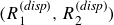 $(R_{1}^{(\textit{disp})},R_{2}^{(\textit{disp})})$
denote the parts of the
$(R_{1}^{(\textit{disp})},R_{2}^{(\textit{disp})})$
denote the parts of the $O(\varepsilon ^3)$
forcing generated by slow modulation (including the
$O(\varepsilon ^3)$
forcing generated by slow modulation (including the $T$
-derivative terms) and other linear dispersive corrections on the chosen scaling. Elasticity enters the triad dynamics only through the acoustic-mode normalisation
$T$
-derivative terms) and other linear dispersive corrections on the chosen scaling. Elasticity enters the triad dynamics only through the acoustic-mode normalisation $\mathcal N_e$
. With the eigenfunction
$\mathcal N_e$
. With the eigenfunction $\varPhi _e(z)$
normalised by
$\varPhi _e(z)$
normalised by $\varPhi _e(0)=1$
, the normalisation decomposes as
$\varPhi _e(0)=1$
, the normalisation decomposes as
 \begin{equation} \mathcal N_e=\mathcal N_{\textit{fs}}+\mathcal N_{\textit{int}}, \end{equation}
where the classical free-surface contribution is
 \begin{equation} \mathcal N_{\textit{fs}} = \int _{-h}^{0}\frac {2\omega }{c^2}|\varPhi _e(z)|^2\mathrm{d} z + \frac {2\omega }{g} |\varPhi _e(0)|^2 = \int _{-h}^{0}\frac {2\omega }{c^2}|\varPhi _e(z)|^2\mathrm{d} z + \frac {2\omega }{g}, \end{equation}
and the elastic interface contribution, arising from the explicit $(\omega ,\kappa )$
-dependence of the impedance boundary operator (2.9), is
$(\omega ,\kappa )$
-dependence of the impedance boundary operator (2.9), is
 \begin{equation} \mathcal N_{\textit{int}} = 2\omega \frac {\partial \mathcal Z}{\partial \omega }(\omega ,\kappa ) |\varPhi _e(-h)|^2. \end{equation}
The term $\mathcal N_{\textit{int}}$
is the direct counterpart of the interface contribution
$\mathcal N_{\textit{int}}$
is the direct counterpart of the interface contribution $\mathcal I_e$
in (5.16) for impedance-type boundary conditions. In the rigid-bottom limit
$\mathcal I_e$
in (5.16) for impedance-type boundary conditions. In the rigid-bottom limit $\mathcal Z\to 0$
smoothly (hence
$\mathcal Z\to 0$
smoothly (hence $\partial _\omega \mathcal Z\to 0$
), so
$\partial _\omega \mathcal Z\to 0$
), so $\mathcal N_{\textit{int}}\to 0$
and
$\mathcal N_{\textit{int}}\to 0$
and $\mathcal N_e\to \mathcal N_{\textit{fs}}$
.
$\mathcal N_e\to \mathcal N_{\textit{fs}}$
.
5.6. Dispersion-derivative identity
An equivalent characterisation of the normalisation follows directly from the elastic dispersion relation $D_e(\omega ,\kappa ;h)=0$
. Differentiating
$D_e(\omega ,\kappa ;h)=0$
. Differentiating $D_e$
with respect to
$D_e$
with respect to $\omega$
, and using the homogeneous eigenproblem for
$\omega$
, and using the homogeneous eigenproblem for $\varPhi _e$
, yields the identity
$\varPhi _e$
, yields the identity
 \begin{equation} \mathcal N_e = \frac {1}{2\omega }\frac {\partial D_e}{\partial \omega }(\omega ,\kappa ;h). \end{equation}
Here, $\partial _\omega D_e$
denotes differentiation with respect to
$\partial _\omega D_e$
denotes differentiation with respect to $\omega$
holding
$\omega$
holding $\kappa$
fixed, and the result is evaluated on the acoustic–gravity branch satisfying
$\kappa$
fixed, and the result is evaluated on the acoustic–gravity branch satisfying $D_e(\omega ,\kappa ;h)=0$
. This is convenient for analysis and confirms that elasticity modifies the triad coefficients through the same object that controls the sensitivity of the acoustic branch to frequency.
$D_e(\omega ,\kappa ;h)=0$
. This is convenient for analysis and confirms that elasticity modifies the triad coefficients through the same object that controls the sensitivity of the acoustic branch to frequency.
6. Energetics and elastic partition of the acoustic mode
The triad evolution equations describe slow-time exchange between two surface gravity wavetrains and a single acoustic–gravity mode supported by the coupled fluid–solid system. It is therefore useful to distinguish between (i) quadratic invariants of the modulation system and (ii) the physical partition of acoustic-mode energy between the fluid and the elastic half-space.
6.1. A conserved quadratic invariant
With weak spatial modulation, the triad system (5.18) possesses a local conservation law. To see this, multiply the acoustic equation by $A^\ast$
, add its complex conjugate, and use
$A^\ast$
, add its complex conjugate, and use
 \begin{align} \partial _T(A^\ast A) + c_e \partial _X(A^\ast A) = A^\ast \big (\mathrm{i}\gamma _e A + \delta _e S_+S_-\big ) + A\big (-\mathrm{i}\gamma _e^\ast A^\ast + \delta _e^\ast S_+^\ast S_-^\ast \big ). \end{align}
This gives
 \begin{equation} \partial _T\big(|A|^2\big) + c_e \partial _X\big(|A|^2\big) = 2\Re \left (\delta _e A^\ast S_+S_-\right ), \end{equation}
where the detuning term contributes only an imaginary part and hence does not affect the balance. Similarly, multiplying the gravity-wave equations by $S_\pm ^\ast$
and adding complex conjugates yields
$S_\pm ^\ast$
and adding complex conjugates yields
 \begin{equation} \partial _T\big(|S_\pm |^2\big) + c_{g\pm } \partial _X\big(|S_\pm |^2\big) = -\Re \left (\delta _e A^\ast S_+S_-\right ). \end{equation}
Summing (6.2) and the two relations (6.3) gives the local conservation law
 \begin{equation} \partial _T\left (|A|^2+|S_+|^2+|S_-|^2\right ) + \partial _X\left (c_e|A|^2+c_{g+}|S_+|^2+c_{g-}|S_-|^2\right ) =0. \end{equation}
In particular, if the envelopes are periodic in $X$
or decay sufficiently rapidly as
$X$
or decay sufficiently rapidly as $|X|\to \infty$
, then integration over
$|X|\to \infty$
, then integration over $X$
shows that
$X$
shows that $\int (|A|^2+|S_+|^2+|S_-|^2 )\mathrm{d} X$
is conserved. This ‘action-like’ conservation law is a standard property of resonant triads and follows from the canonical structure of the modulation equations. It does not, by itself, specify how the acoustic-mode physical energy is distributed between the fluid and the solid.
$\int (|A|^2+|S_+|^2+|S_-|^2 )\mathrm{d} X$
is conserved. This ‘action-like’ conservation law is a standard property of resonant triads and follows from the canonical structure of the modulation equations. It does not, by itself, specify how the acoustic-mode physical energy is distributed between the fluid and the solid.
6.2. Physical acoustic-mode energy and elastic partition
The physical quadratic energy associated with the acoustic–gravity mode is proportional to the normalisation arising from the solvability condition. With the eigenfunction normalised by $\varPhi _e(0)=1$
, the mode energy may be written (up to a constant prefactor) as
$\varPhi _e(0)=1$
, the mode energy may be written (up to a constant prefactor) as
 \begin{equation} E_e^{\textit{phys}} \propto ( \mathcal N_{\textit{fs}}+\mathcal N_{\textit{int}}) |A|^2, \end{equation}
where $\mathcal N_{\textit{fs}}$
and
$\mathcal N_{\textit{fs}}$
and $\mathcal N_{\textit{int}}$
are given explicitly by (5.23)–(5.24). For impedance conditions of the form
$\mathcal N_{\textit{int}}$
are given explicitly by (5.23)–(5.24). For impedance conditions of the form $\phi _{l,z}-\mathcal Z(\omega ,\kappa )\phi _l=0$
, the interface contribution to the frequency normalisation arises from the
$\phi _{l,z}-\mathcal Z(\omega ,\kappa )\phi _l=0$
, the interface contribution to the frequency normalisation arises from the $\omega$
-sensitivity of the boundary operator (equivalently, from
$\omega$
-sensitivity of the boundary operator (equivalently, from $\partial _\omega D_e$
), while
$\partial _\omega D_e$
), while $\kappa$
-dependence enters the detuning/dispersion corrections through the elastic dispersion relation
$\kappa$
-dependence enters the detuning/dispersion corrections through the elastic dispersion relation $D_e(\omega ,\kappa ;h)$
and is accounted for in
$D_e(\omega ,\kappa ;h)$
and is accounted for in $\mathcal D$
and
$\mathcal D$
and $\beta$
. This decomposition provides a natural energetic interpretation
$\beta$
. This decomposition provides a natural energetic interpretation
 \begin{equation} E_{e,f}^{\textit{phys}} \propto \mathcal N_{\textit{fs}}|A|^2, \qquad E_{e,s}^{\textit{phys}} \propto \mathcal N_{\textit{int}}|A|^2, \end{equation}
where $E_{e,f}^{\textit{phys}}$
is the fluid-associated contribution (bulk plus free surface), while
$E_{e,f}^{\textit{phys}}$
is the fluid-associated contribution (bulk plus free surface), while $E_{e,s}^{\textit{phys}}$
measures the portion of the acoustic-mode energy stored in (or transmitted into) the elastic half-space through the impedance operator.
$E_{e,s}^{\textit{phys}}$
measures the portion of the acoustic-mode energy stored in (or transmitted into) the elastic half-space through the impedance operator.
In the rigid-bottom limit $\mathcal Z\to 0$
,
$\mathcal Z\to 0$
, $\mathcal N_{\textit{int}}\to 0$
and the acoustic-mode energy is entirely contained in the fluid. For an elastic half-space,
$\mathcal N_{\textit{int}}\to 0$
and the acoustic-mode energy is entirely contained in the fluid. For an elastic half-space, $\mathcal N_{\textit{int}}$
is generally non-zero and quantifies the degree of elastic participation in the acoustic–gravity mode.
$\mathcal N_{\textit{int}}$
is generally non-zero and quantifies the degree of elastic participation in the acoustic–gravity mode.
6.3. Energetic meaning of ‘elastic leakage’
The present model is conservative: in the absence of attenuation, energy transferred into the elastic half-space is not lost but becomes part of the coupled fluid–solid mode. In that sense, elasticity does not dissipate triad energy; it redistributes the acoustic-mode energy between the fluid and the solid according to (6.6). If weak attenuation in the solid is included (not considered here), the same partition determines the fraction of triad-fed acoustic energy that is subsequently dissipated in the solid bottom boundary.
In the lossless elastic half-space considered here, the impedance is taken to be real on the branches analysed, so the triad system remains conservative. If attenuation in the solid is included, the effective impedance becomes complex and the modulation equations would acquire genuine decay on the slow time scale.
7. Discussion and conclusions
A central outcome of the present analysis is a clear separation between two distinct roles played by elasticity (and, more generally, compressibility-mediated bottom compliance) in acoustic–gravity wave triad resonance. These roles correspond to two mathematically different regimes of the underlying dispersion problem.
7.1. Regular regime: perturbative effect when the rigid-bottom triad exists
When the acoustic–gravity wave member of the triad exists in the rigid-bottom formulation, the corresponding dispersion relation
 \begin{equation} D_r(\omega ,\kappa ;h)=0 \end{equation}
admits a simple real root $(\omega _0,\kappa _0)$
, satisfying
$(\omega _0,\kappa _0)$
, satisfying
 \begin{equation} \frac {\partial D_r}{\partial \omega }(\omega _0,\kappa _0;h)\neq 0. \end{equation}
In this case, the elastic-bottom dispersion relation derived in the present work may be written in the form
 \begin{equation} D_e(\omega ,\kappa ;h) = D_r(\omega ,\kappa ;h) + \mathcal Z(\omega ,\kappa )Q(\omega ,\kappa ;h), \end{equation}
where $\mathcal Z$
is the effective elastic impedance and
$\mathcal Z$
is the effective elastic impedance and $Q$
is given explicitly by (3.10).
$Q$
is given explicitly by (3.10).
By the implicit function theorem, (7.3) admits a unique nearby root
 \begin{equation} \omega _e(\kappa )=\omega _0(\kappa )+O(\mathcal Z), \end{equation}
and hence the elastic correction to the acoustic–gravity wave frequency is perturbatively small. Using the dispersion-derivative identity (5.25) established in § 5.6, the elastic normalisation satisfies
 \begin{equation} \mathcal N_e = \frac {1}{2\omega }\frac {\partial D_e}{\partial \omega } = \mathcal N_r\big (1+O(\mathcal Z)\big ), \end{equation}
where $\mathcal N_r=(2\omega )^{-1}\partial _\omega D_r$
is the rigid-bottom normalisation.
$\mathcal N_r=(2\omega )^{-1}\partial _\omega D_r$
is the rigid-bottom normalisation.
Since the quadratic forcing responsible for the triad interaction arises solely from free-surface nonlinearities, the coupling coefficient in the elastic case retains the form
 \begin{equation} \delta _e=\frac {\mathcal P}{\mathcal N_e}, \end{equation}
where $\mathcal P$
is the same quadratic projection coefficient as in the rigid-bottom theory and is therefore independent of the bottom model at the order considered. Denoting by
$\mathcal P$
is the same quadratic projection coefficient as in the rigid-bottom theory and is therefore independent of the bottom model at the order considered. Denoting by
 \begin{equation} \delta _r=\frac {\mathcal P}{\mathcal N_r} \end{equation}
the corresponding rigid-bottom coupling coefficient, we obtain
 \begin{equation} \frac {\delta _e}{\delta _r}=\frac {\mathcal N_r}{\mathcal N_e}=1+O(\mathcal Z). \end{equation}
Hence, when the rigid-bottom triad already exists, elasticity produces only a perturbatively small correction to the coupling strength, and therefore to the associated growth rate and slow modulation dynamics. In this regular regime, elasticity acts as a weak correction to the classical rigid-bottom theory.
7.2. Singular regime: elasticity as a mechanism for admitting triad resonance
A fundamentally different situation arises near the rigid-bottom cutoff. In shallow configurations, the rigid-bottom dispersion relation ceases to admit a propagating acoustic–gravity wave solution; mathematically, this corresponds to a degeneracy characterised by
 \begin{equation} D_r(\omega _c,\kappa _c;h_c)=0, \qquad \frac {\partial D_r}{\partial \omega }(\omega _c,\kappa _c;h_c)=0. \end{equation}
At such points, the rigid-bottom acoustic–gravity wave branch terminates and no triad closure is possible.
Near the cutoff, the rigid dispersion relation has a non-degenerate turning-point expansion
 \begin{equation} D_r \approx \frac {1}{2}D_{\omega \omega }(\omega _c,\kappa _c;h_c)(\omega -\omega _c)^2 + D_h(\omega _c,\kappa _c;h_c)(h-h_c), \end{equation}
with $D_{\omega \omega }(\omega _c,\kappa _c;h_c)\neq 0$
at this first cutoff. The cutoff-shift argument below depends only on this non-degeneracy, not on the sign of
$D_{\omega \omega }(\omega _c,\kappa _c;h_c)\neq 0$
at this first cutoff. The cutoff-shift argument below depends only on this non-degeneracy, not on the sign of $D_{\omega \omega }$
. Since the elastic contribution enters additively through
$D_{\omega \omega }$
. Since the elastic contribution enters additively through $\mathcal ZQ$
, the perturbed cutoff is obtained by setting
$\mathcal ZQ$
, the perturbed cutoff is obtained by setting $D_e=0$
, which yields the leading-order shift
$D_e=0$
, which yields the leading-order shift
 \begin{equation} h_c^{(e)}-h_c^{(r)} \approx -\frac {\mathcal Z(\omega _c,\kappa _c)Q(\omega _c,\kappa _c;h_c)}{D_h(\omega _c,\kappa _c;h_c)}. \end{equation}
For the first rigid cutoff (with $\kappa \simeq 0$
), one has
$\kappa \simeq 0$
), one has $\alpha h=\pi /2$
, so
$\alpha h=\pi /2$
, so $\cos (\alpha h)=0$
and
$\cos (\alpha h)=0$
and $\sin (\alpha h)=1$
. At this point
$\sin (\alpha h)=1$
. At this point
 \begin{align} Q(\omega _c,\kappa _c;h_c)= -\frac {\omega _c^2}{\alpha _c}\lt 0, \qquad D_h(\omega _c,\kappa _c;h_c)=\partial _h D_r = \omega _c^2\alpha _c\gt 0, \end{align}
so $Q/D_h\lt 0$
. For the conservative weak-coupling branch considered here, Appendix A shows that
$Q/D_h\lt 0$
. For the conservative weak-coupling branch considered here, Appendix A shows that $\mathcal Z(\omega _c,\kappa _c)\lt 0$
. Hence,
$\mathcal Z(\omega _c,\kappa _c)\lt 0$
. Hence, $\mathcal Z\,Q\gt 0$
and (7.11) gives
$\mathcal Z\,Q\gt 0$
and (7.11) gives $h_c^{(e)}-h_c^{(r)}\lt 0$
: elastic coupling reduces the cutoff depth, consistent with the physical picture that a compliant interface restores a guided acoustic–gravity mode in shallower configurations.
$h_c^{(e)}-h_c^{(r)}\lt 0$
: elastic coupling reduces the cutoff depth, consistent with the physical picture that a compliant interface restores a guided acoustic–gravity mode in shallower configurations.
Thus, even weak elastic coupling can restore a propagating acoustic–gravity wave mode in depth regimes where the rigid-bottom theory predicts evanescence. In this singular regime, elasticity does not merely perturb an existing triad; it alters the very admissibility of the acoustic member and thereby enables triad resonance. This distinction is reflected directly in the solvability condition derived in the present work. The elastic interface contribution to the normalisation
 \begin{equation} \mathcal N_{\textit{int}} = 2\omega \frac {\partial \mathcal Z}{\partial \omega }|\varPhi _e(-h)|^2, \end{equation}
vanishes in the rigid limit but becomes dynamically significant precisely when the rigid-bottom normalisation degenerates near cutoff. Physically, this term represents the exchange of energy between the fluid and the compliant seabed (or more generally bottom boundary), which becomes decisive when the acoustic mode is marginally trapped.
7.3. Experimental feasibility and laboratory-scale realisation
The removal of the rigid-bottom cutoff by elastic coupling has a direct experimental implication: resonant triads can be realised at significantly smaller depths and frequencies than required over a rigid bed. For example, in a laboratory tank with $h\sim 0.2$
–
$h\sim 0.2$
– $0.5\, \mathrm{m}$
one can generate nearly counter-propagating gravity wavetrains with
$0.5\, \mathrm{m}$
one can generate nearly counter-propagating gravity wavetrains with $k\sim 6$
–
$k\sim 6$
– $10\, \mathrm{m^{-1}}$
(wavelengths
$10\, \mathrm{m^{-1}}$
(wavelengths $\lambda \sim 0.6$
–
$\lambda \sim 0.6$
– $1.0\, \mathrm{m}$
) and frequencies
$1.0\, \mathrm{m}$
) and frequencies $f\sim 1$
–
$f\sim 1$
– $2\, \mathrm{Hz}$
, so that the triad acoustic–gravity frequency is
$2\, \mathrm{Hz}$
, so that the triad acoustic–gravity frequency is $f\sim 2$
–
$f\sim 2$
– $4\, \mathrm{Hz}$
. Under rigid-bottom conditions the corresponding acoustic–gravity mode may be evanescent in such shallow configurations, whereas a compliant substrate (approximating an elastic half-space) can support an interface-guided acoustic–gravity branch that remains admissible. This increases the feasibility of controlled laboratory measurements of triad-driven energy exchange, including direct interrogation of the coupling and detuning coefficients through envelope dynamics. However, practical realisation of the nonlinear triad resonance in laboratory conditions is not guaranteed.
$4\, \mathrm{Hz}$
. Under rigid-bottom conditions the corresponding acoustic–gravity mode may be evanescent in such shallow configurations, whereas a compliant substrate (approximating an elastic half-space) can support an interface-guided acoustic–gravity branch that remains admissible. This increases the feasibility of controlled laboratory measurements of triad-driven energy exchange, including direct interrogation of the coupling and detuning coefficients through envelope dynamics. However, practical realisation of the nonlinear triad resonance in laboratory conditions is not guaranteed.
7.4. Practical feasibility maps
Admissibility of an elastic acoustic–gravity branch is a necessary condition for triad resonance, but it does not by itself indicate whether the resulting acoustic signal is measurable in a finite facility. In the present paper, all feasibility calculations are restricted to the conservative guided branches described in Appendix A; radiating or leaky branches are excluded from the weakly nonlinear framework adopted here. To connect the theory to observability, we introduce the detection margin $\mathcal M\equiv p_{\textit{cap}}/p_{\textit{detect}}$
, where
$\mathcal M\equiv p_{\textit{cap}}/p_{\textit{detect}}$
, where $p_{\textit{cap}}$
is the acoustic pressure predicted to be reached within the available interaction time and
$p_{\textit{cap}}$
is the acoustic pressure predicted to be reached within the available interaction time and $p_{\textit{detect}}$
is a nominal detection threshold. For each candidate configuration, the acoustic member of the triad is obtained from the full elastic dispersion relation (3.7), and its modal normalisation is evaluated using the dispersion-derivative identity (5.25). The operating point is then optimised over admissible depths
$p_{\textit{detect}}$
is a nominal detection threshold. For each candidate configuration, the acoustic member of the triad is obtained from the full elastic dispersion relation (3.7), and its modal normalisation is evaluated using the dispersion-derivative identity (5.25). The operating point is then optimised over admissible depths $h\leqslant H_{max }^{\textit{req}}$
and acoustic frequencies below a prescribed gravity–capillary safety limit, while enforcing a weakly nonlinear validity cap on the forcing amplitude. The available interaction time is taken as the smaller of the viscous damping time and the flume transit time.
$h\leqslant H_{max }^{\textit{req}}$
and acoustic frequencies below a prescribed gravity–capillary safety limit, while enforcing a weakly nonlinear validity cap on the forcing amplitude. The available interaction time is taken as the smaller of the viscous damping time and the flume transit time.
Optimisation over realistic fluid–solid pairs shows that detectability improves strongly with both flume length $L$
and maximum usable depth
$L$
and maximum usable depth $H_{max }^{\textit{req}}$
(see figure 2), with depth emerging as the dominant control parameter over the range examined, i.e. shallow facilities remain well below threshold across the range of
$H_{max }^{\textit{req}}$
(see figure 2), with depth emerging as the dominant control parameter over the range examined, i.e. shallow facilities remain well below threshold across the range of $L$
, whereas sufficiently deep facilities become plausible even at moderate lengths (figure 2
a). Relaxing the weak-nonlinearity cap (from
$L$
, whereas sufficiently deep facilities become plausible even at moderate lengths (figure 2
a). Relaxing the weak-nonlinearity cap (from $\alpha \leqslant 1$
to
$\alpha \leqslant 1$
to $\alpha \leqslant 2$
) reduces the minimum depth needed for
$\alpha \leqslant 2$
) reduces the minimum depth needed for $\mathcal M\gtrsim 1$
(figure 2
b), but does not change the basic conclusion that depth is the primary control parameter, with
$\mathcal M\gtrsim 1$
(figure 2
b), but does not change the basic conclusion that depth is the primary control parameter, with $L$
entering mainly through the available interaction time.
$L$
entering mainly through the available interaction time.
Since small/medium flumes seem to be practically unfavourable for the sought triad-resonance experiment, we next focus attention on large water flumes (with water as the working fluid), varying only the substrate within the material catalogue considered here; the facility dimensions used as constraints are listed in table 1. Under the stricter cap $\alpha \leqslant 1$
, the deepest facilities provide the best prospects, while more limited depths remain below threshold even with favourable substrates (figure 3
a). Increasing
$\alpha \leqslant 1$
, the deepest facilities provide the best prospects, while more limited depths remain below threshold even with favourable substrates (figure 3
a). Increasing $\alpha _{max }$
can move marginal cases toward detectability, but it does not eliminate the strong ordering with facility depth (figure 3
b). Thus, although elasticity removes the rigid-bottom cutoff and enlarges the admissible triad parameter space, the more stringent practical conclusion is that an observable signal in water still requires very large and, especially, deep facilities; variations in substrate properties provide only secondary improvement compared with increasing usable depth.
$\alpha _{max }$
can move marginal cases toward detectability, but it does not eliminate the strong ordering with facility depth (figure 3
b). Thus, although elasticity removes the rigid-bottom cutoff and enlarges the admissible triad parameter space, the more stringent practical conclusion is that an observable signal in water still requires very large and, especially, deep facilities; variations in substrate properties provide only secondary improvement compared with increasing usable depth.
Generic facility-scale feasibility for observing acoustic–gravity triad resonance. (a) Detection margin $\log _{10}\mathcal M$
in the
$\log _{10}\mathcal M$
in the $(L,\,H_{max }^{\textit{req}})$
plane, after optimisation over admissible operating conditions and realistic Newtonian fluid–solid pairs; the dashed contour marks
$(L,\,H_{max }^{\textit{req}})$
plane, after optimisation over admissible operating conditions and realistic Newtonian fluid–solid pairs; the dashed contour marks $\mathcal M=1$
for the stricter cap
$\mathcal M=1$
for the stricter cap $\alpha \leqslant 1$
. (b) Minimum required depth
$\alpha \leqslant 1$
. (b) Minimum required depth $H_{max }^{\textit{req}}$
versus flume length
$H_{max }^{\textit{req}}$
versus flume length $L$
for two weak-nonlinearity caps,
$L$
for two weak-nonlinearity caps, $\alpha \leqslant 1$
and
$\alpha \leqslant 1$
and $\alpha \leqslant 2$
.
$\alpha \leqslant 2$
.

Large experimental water flumes considered in the water-only facility analysis. Here, $L$
is the flume length,
$L$
is the flume length, $W$
is the quoted width and
$W$
is the quoted width and $H_{max }^{\textit{req}}$
is the maximum stated operating water depth used as the upper depth constraint in the feasibility calculations.
$H_{max }^{\textit{req}}$
is the maximum stated operating water depth used as the upper depth constraint in the feasibility calculations.

Water-only feasibility in selected large flumes, computed as in § 7.4. (a) Detection margin $\log _{10}\mathcal M$
for each flume–substrate pair under the stricter cap
$\log _{10}\mathcal M$
for each flume–substrate pair under the stricter cap $\alpha \leqslant 1$
; open squares indicate the best substrate within each flume and the star denotes the overall best case. Hatched columns indicate substrates for which no conservative guided branch exists in the present model (
$\alpha \leqslant 1$
; open squares indicate the best substrate within each flume and the star denotes the overall best case. Hatched columns indicate substrates for which no conservative guided branch exists in the present model ( $C_s\leqslant c$
, so the interval
$C_s\leqslant c$
, so the interval $\omega /C_s\lt \kappa \lt \omega /c$
is empty). (b) Optimised detection margin versus
$\omega /C_s\lt \kappa \lt \omega /c$
is empty). (b) Optimised detection margin versus $\alpha _{max }$
for each flume, maximised over admissible
$\alpha _{max }$
for each flume, maximised over admissible $(h,f)$
and over the valid substrate set.
$(h,f)$
and over the valid substrate set.

Figure 3. Long description
The image contains two graphs. Panel A: A heatmap graph shows the detection margin for each flume-substrate pair under a stricter cap. The x-axis represents solid substrates with speeds in kilometers per second, and the y-axis represents actual water flumes with maximum heights in meters. The color scale indicates the log of the detection margin, with darker colors representing lower margins. Open squares mark the best substrate within each flume, and a star denotes the overall best case. Hatched columns indicate substrates for which no conservative guided branch exists. Panel B: A line graph shows the optimized detection margin versus the weak-nonlinearity cap for each flume, maximized over admissible values and valid substrate sets. The x-axis represents the weak-nonlinearity cap, and the y-axis represents the detection margin on a logarithmic scale. Different colored lines represent different flumes, with labels indicating the flume names and their maximum heights.
7.5. Outlook
Several directions for future work emerge naturally from the present study. A systematic evaluation of the elastic impedance for realistic bottom boundary materials would enable mapping of admissible triads and coefficient variations across parameter space. Incorporating weak attenuation in the solid would quantify how elastic participation, measured by $\mathcal N_{\textit{int}}/\mathcal N_e$
, translates into measurable decay of acoustic energy in long-time dynamics. It is worth noting that the analysis presented here follows the triad setting of Kadri & Akylas (Reference Kadri and Akylas2016); in regimes where the acoustic horizontal length scale is much larger than the water depth, a different asymptotic ordering applies and the corresponding evolution equations would need to be re-derived. Finally, extension to acoustic–gravity-capillary triad resonance, three-dimensional geometries, and layered or poroelastic bottom structures would broaden applicability to laboratory experiments, coastal acoustics and geophysical settings.
$\mathcal N_{\textit{int}}/\mathcal N_e$
, translates into measurable decay of acoustic energy in long-time dynamics. It is worth noting that the analysis presented here follows the triad setting of Kadri & Akylas (Reference Kadri and Akylas2016); in regimes where the acoustic horizontal length scale is much larger than the water depth, a different asymptotic ordering applies and the corresponding evolution equations would need to be re-derived. Finally, extension to acoustic–gravity-capillary triad resonance, three-dimensional geometries, and layered or poroelastic bottom structures would broaden applicability to laboratory experiments, coastal acoustics and geophysical settings.
Acknowledgements
This work was supported by the Leverhulme Trust Research Project Grant number 523930. AI tools were used for language editing; and all scientific content, analysis, and conclusions are the author’s own.
Declaration of interests
The author reports no conflict of interest.
Data availability statement
The data that support the findings of this study are available from the corresponding author upon reasonable request.
Appendix A. Elastic half-space impedance and dispersion relation
For completeness, we present the effective impedance condition at the fluid–elastic solid interface for a homogeneous isotropic elastic half-space and the resulting finite-depth acoustic–gravity dispersion relation. The detailed elimination of the elastic potentials is given in Eyov et al. (Reference Eyov, Klar, Kadri and Stiassnie2013); here we present the final expressions in the notation of the present paper.
A.1. Governing equations in the solid
In the elastic half-space $z\leqslant -h$
, the displacement
$z\leqslant -h$
, the displacement $\boldsymbol u_s=(u_s,w_s)$
satisfies linear elasticity
$\boldsymbol u_s=(u_s,w_s)$
satisfies linear elasticity
 \begin{equation} \rho _s \boldsymbol u_{s,tt} = (\lambda _s+\mu _s)\boldsymbol{\nabla }(\boldsymbol{\nabla }\boldsymbol{\cdot }\boldsymbol u_s) + \mu _s \boldsymbol{\nabla} ^2 \boldsymbol u_s, \end{equation}
where $\rho _s$
is the solid density and
$\rho _s$
is the solid density and $(\lambda _s,\mu _s)$
are Lamé parameters. Introducing scalar and vector potentials
$(\lambda _s,\mu _s)$
are Lamé parameters. Introducing scalar and vector potentials $\phi _s$
and
$\phi _s$
and $\boldsymbol \psi _s=(0,\psi _s,0)$
 \begin{equation} \boldsymbol u_s=\boldsymbol{\nabla }\phi _s+\boldsymbol{\nabla }\times \boldsymbol \psi _s, \end{equation}
the potentials satisfy
 \begin{equation} \boldsymbol{\nabla} ^2\phi _s=\frac {1}{C_p^2}\phi _{s,tt}, \qquad \boldsymbol{\nabla} ^2\psi _s=\frac {1}{C_s^2}\psi _{s,tt}, \end{equation}
with compressional and shear speeds $C_p=\sqrt {(\lambda _s+2\mu _s)/\rho _s}$
and
$C_p=\sqrt {(\lambda _s+2\mu _s)/\rho _s}$
and $C_s=\sqrt {\mu _s/\rho _s}$
.
$C_s=\sqrt {\mu _s/\rho _s}$
.
A.1. Spectral variables
We consider two-dimensional time-harmonic dependence $\exp \{\mathrm{i}(\kappa x-\omega t)\}$
. In the fluid
$\exp \{\mathrm{i}(\kappa x-\omega t)\}$
. In the fluid
 \begin{equation} \varPhi _{zz}+\alpha ^2\varPhi =0, \qquad \alpha ^2=\frac {\omega ^2}{c^2}-\kappa ^2, \qquad -h\leqslant z\leqslant 0, \end{equation}
and the linear free-surface condition is
 \begin{equation} g\varPhi _z-\omega ^2\varPhi =0, \qquad z=0. \end{equation}
We take the branch $\alpha =\sqrt {\omega ^2/c^2-\kappa ^2}$
with
$\alpha =\sqrt {\omega ^2/c^2-\kappa ^2}$
with $\Re (\alpha )\geqslant 0$
.
$\Re (\alpha )\geqslant 0$
.
In the elastic half-space, decay as $z\to -\infty$
introduces the vertical wavenumbers
$z\to -\infty$
introduces the vertical wavenumbers
 \begin{equation} q_p=\sqrt {\kappa ^2-\frac {\omega ^2}{C_p^2}}, \qquad q_s=\sqrt {\kappa ^2-\frac {\omega ^2}{C_s^2}}, \end{equation}
with square-root branches chosen such that $\Re (q_p)\gt 0$
and
$\Re (q_p)\gt 0$
and $\Re (q_s)\gt 0$
(so that the elastic fields decay as
$\Re (q_s)\gt 0$
(so that the elastic fields decay as $z\to -\infty$
). In the present lossless setting we focus on real
$z\to -\infty$
). In the present lossless setting we focus on real $\omega$
and
$\omega$
and $\kappa$
on conservative (non-radiating) branches of the coupled dispersion relation. Depending on
$\kappa$
on conservative (non-radiating) branches of the coupled dispersion relation. Depending on $(\omega ,\kappa )$
,
$(\omega ,\kappa )$
, $q_p$
and/or
$q_p$
and/or $q_s$
may be complex; this corresponds to radiating/leaky behaviour in the half-space and is not pursued here, since the weakly nonlinear triad reduction is formulated for the conservative (Hamiltonian) regime.
$q_s$
may be complex; this corresponds to radiating/leaky behaviour in the half-space and is not pursued here, since the weakly nonlinear triad reduction is formulated for the conservative (Hamiltonian) regime.
A.3. Exact impedance boundary condition at $z=-h$

Imposing continuity of vertical velocity and normal traction, together with vanishing shear traction at the interface (liquid cannot support shear), the elastic variables may be eliminated to give an effective impedance condition on the fluid potential
 \begin{equation} \phi _{l,z}-\mathcal Z(\omega ,\kappa )\phi _l=0, \qquad z=-h. \end{equation}
The exact half-space impedance may be written as
 \begin{equation} \mathcal Z(\omega ,\kappa )= \underbrace {\frac {\rho _l \omega ^2}{\rho _s}\frac {q_p}{\omega ^2-C_s^2\kappa ^2}}_{\displaystyle \mathcal Z_{\textit{lead}}(\omega ,\kappa )} \times \underbrace {\mathcal F(\omega ,\kappa )}_{\displaystyle \text{dimensionless correction}}, \end{equation}
where $\mathcal Z_{\textit{lead}}$
gives the leading impedance scaling obtained by eliminating the elastic potentials (up to the sign convention implied by
$\mathcal Z_{\textit{lead}}$
gives the leading impedance scaling obtained by eliminating the elastic potentials (up to the sign convention implied by $\exp \{\mathrm{i}(\kappa x-\omega t)\}$
and the definition of normal traction), and
$\exp \{\mathrm{i}(\kappa x-\omega t)\}$
and the definition of normal traction), and $\mathcal F$
is a dimensionless correction accounting for shear coupling and mode conversion in the half-space
$\mathcal F$
is a dimensionless correction accounting for shear coupling and mode conversion in the half-space
 \begin{equation} \mathcal F(\omega ,\kappa ) =\frac {1}{1+4\kappa ^2 q_p q_s\left (\omega ^2/C_s^2-2\kappa ^2\right )^{-2}} \frac {\kappa ^2+q_s^2}{\kappa ^2-q_s^2}. \end{equation}
In the conservative guided regime considered here (real $\omega ,\kappa$
with decaying elastic fields), the effective impedance is real. With the present sign convention,
$\omega ,\kappa$
with decaying elastic fields), the effective impedance is real. With the present sign convention, $\mathcal Z_{\textit{lead}}$
is negative when
$\mathcal Z_{\textit{lead}}$
is negative when $q_p$
is real and
$q_p$
is real and $\kappa ^2\gt \omega ^2/C_s^2$
; in the weak-coupling guided branches examined in this paper, the full impedance
$\kappa ^2\gt \omega ^2/C_s^2$
; in the weak-coupling guided branches examined in this paper, the full impedance $\mathcal Z$
has the same sign.
$\mathcal Z$
has the same sign.
Using $\kappa ^2-q_s^2=\omega ^2/C_s^2$
allows
$\kappa ^2-q_s^2=\omega ^2/C_s^2$
allows $\mathcal Z$
to be written explicitly as
$\mathcal Z$
to be written explicitly as
 \begin{equation} \mathcal Z(\omega ,\kappa ) =-\frac {\rho _l}{\rho _s}\frac {q_p\,(\kappa ^2+q_s^2)}{\kappa ^2-\omega ^2/C_s^2} \left [1+4\kappa ^2 q_p q_s\left (\omega ^2/C_s^2-2\kappa ^2\right )^{-2}\right ]^{-1}. \end{equation}
Equivalently, since $\kappa ^2+q_s^2=2\kappa ^2-\omega ^2/C_s^2$
, (A10) may be written entirely in terms of
$\kappa ^2+q_s^2=2\kappa ^2-\omega ^2/C_s^2$
, (A10) may be written entirely in terms of $(\omega ,\kappa )$
as
$(\omega ,\kappa )$
as
 \begin{equation} \mathcal Z(\omega ,\kappa )=-\frac {\rho _l}{\rho _s}\frac {\sqrt {\kappa ^2-\frac {\omega ^2}{C_p^2}}\left (2\kappa ^2-\frac {\omega ^2}{C_s^2}\right )}{\kappa ^2-\frac {\omega ^2}{C_s^2}}\left [1+\frac {4\kappa ^2\sqrt {\kappa ^2-\frac {\omega ^2}{C_p^2}}\sqrt {\kappa ^2-\frac {\omega ^2}{C_s^2}}}{\left (\frac {\omega ^2}{C_s^2}-2\kappa ^2\right )^2}\right ]^{-1}. \end{equation}
Equations (A7)–(A11) are algebraically equivalent to the half-space reduction in Eyov et al. (Reference Eyov, Klar, Kadri and Stiassnie2013), rewritten in the present notation.
A.4. Finite-depth dispersion relation
Combining the fluid eigenproblem, the free-surface condition, and the impedance boundary condition yields the dispersion relation used in the main text
 \begin{align} D_e(\omega ,\kappa ;h)&\equiv g\big [-\alpha \sin (\alpha h)+\mathcal Z(\omega ,\kappa )\cos (\alpha h)\big ] -\omega ^2\Big [\cos (\alpha h)+\frac {\mathcal Z(\omega ,\kappa )}{\alpha }\sin (\alpha h)\Big ]\notag\\& =0. \end{align}
Appendix B. Recovery of the rigid-bottom resonant-triad framework
For completeness, we show explicitly how the present formulation reduces to the classical rigid-bottom acoustic–gravity resonant-triad framework in the appropriate limit. In the rigid-bottom case, the interface condition reduces to
 \begin{equation} \phi _{l,z} = 0, \qquad z=-h . \end{equation}
With the impedance convention (2.9), this corresponds to the limit $\mathcal Z\to 0$
. The boundary operator
$\mathcal Z\to 0$
. The boundary operator $\mathcal{B}_e$
is independent of spectral parameters, and hence
$\mathcal{B}_e$
is independent of spectral parameters, and hence
 \begin{equation} \partial _\omega \mathcal{B}_e = \partial _\kappa \mathcal{B}_e = 0. \end{equation}
As a result, the interface contribution $\mathcal{I}_e$
in the solvability condition vanishes identically. The acoustic-mode normalisation reduces to the classical free-surface contribution
$\mathcal{I}_e$
in the solvability condition vanishes identically. The acoustic-mode normalisation reduces to the classical free-surface contribution
 \begin{equation} \mathcal{N}_e \to \mathcal{N}_{\textit{fs}}, \end{equation}
and the coupling and detuning coefficients recover their rigid-bottom forms. The triad evolution equations and their associated invariants coincide with those obtained in previous rigid-bottom analyses.
Appendix C. Large experimental water flumes used in the feasibility analysis
For the feasibility analysis in § 7.4, we considered a set of large hydraulic and coastal research flumes whose publicly stated lengths and maximum water depths are sufficiently well documented to define practical facility constraints. In each case, the flume length $L$
was used in the transit-time estimate, while the maximum usable water depth
$L$
was used in the transit-time estimate, while the maximum usable water depth $H_{max }^{\textit{req}}$
was used as the upper bound in the depth optimisation. The quoted widths are included for context only and were not used explicitly in the present one-dimensional observability proxy. Because public descriptions of these facilities are not perfectly uniform, the values in table 1 should be interpreted as practical working dimensions rather than as a strict ranking by geometric volume.
$H_{max }^{\textit{req}}$
was used as the upper bound in the depth optimisation. The quoted widths are included for context only and were not used explicitly in the present one-dimensional observability proxy. Because public descriptions of these facilities are not perfectly uniform, the values in table 1 should be interpreted as practical working dimensions rather than as a strict ranking by geometric volume.

 h=0.30,m
 ω/κ
ω/κ ω
ω ω>ωc=πc/(2h)
 ωc
ωc κ(ω)
κ(ω) ωgc
ωgc
 log10M
 (L,Hmaxreq)
 M=1
M=1 α⩽1
α⩽1 Hmaxreq
 L
L α⩽1
α⩽1 α⩽2
α⩽2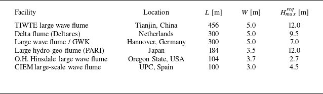
 L
L W
W Hmaxreq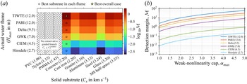
 log10M
 α⩽1
α⩽1 Cs⩽c
Cs⩽c ω/Cs<κ<ω/c
 αmax
αmax (h,f)
(h,f)
 Open access

