





1. Introduction
Vortices and waves are arguably the most important building blocks of complex fluid flows. The evolution and dynamics of vortices in interface flows and in particular the associated wave–vortex interactions constitute a major canonical problem in fluid dynamics (Bühler Reference Bühler2010; McIntyre Reference McIntyre2019). Important applications range from naval hydrodynamics (Sarpkaya & Neubert Reference Sarpkaya and Neubert1994; Chen & Chwang Reference Chen and Chwang2002; Curtis & Kalisch Reference Curtis and Kalisch2017) over aeronautics (Sarpkaya & Suthon Reference Sarpkaya and Suthon1991) to geophysics (Bühler Reference Bühler2010; van Heijst Reference van Heijst2017). This prior research focused on vortices close to free surfaces, emphasising surface deformation processes (Curtis & Kalisch Reference Curtis and Kalisch2017), vortex instabilities (Archer, Thomas & Coleman Reference Archer, Thomas and Coleman2010), wave refraction (Bühler Reference Bühler2010; McIntyre Reference McIntyre2019) and interface entrainment (Linden Reference Linden1973). Probably for reasons of experimental realisability and theoretical tractability, prior studies assumed (self-rising) vortex rings, two-dimensional vortex pairs or point vortices. In this study, we investigate the three-dimensional dynamics of an isolated line vortex that can be assumed sufficiently far from a free surface so as not to exert any appreciable effect on the free-surface wave dynamics. However, the surface impacts the vortex dynamics through a time-dependent boundary condition in the surrounding potential-flow field.
More specifically, this study focuses on the unsteady dynamics of a single slender line vortex, as it forms, e.g. in the wake of a lifting surface, perpetually excited by small-scale turbulence and free-surface gravity-wave flow. Besides potential relevance in the above applications, this is also an important abstraction of vortex experiments conducted in free-surface water channels (Baker et al. Reference Baker, Barker, Bofah and Saffman1974; Bailey et al. Reference Bailey, Pentelow, Ghimire, Estejab, Green and Tavoularis2018; Gutierrez-Castillo et al. Reference Gutierrez-Castillo, Garrido-Martin, Bölle, García-Ortiz, Aguilar-Cabello and del Pino2022). In this setting, the vortex axis and the direction of wave propagation are aligned. The main manifestation of unsteady vortex dynamics observed in such experiments of line vortices is referred to as meandering (Jacquin et al. Reference Jacquin, Fabre, Geffroy and Coustols2001; Bölle Reference Bölle2021). Despite numerous studies, its root cause and governing mechanisms are not fully understood (Edstrand et al. Reference Edstrand, Davis, Schmid, Taira and Cattafesta2016; Bölle Reference Bölle2023; Wu et al. Reference Wu, Xiao, Xiang, Li and Liu2025). Candidate mechanisms have been reviewed and critically discussed recently by Bölle (Reference Bölle2024).
While there is no rigorous definition of vortex meandering, it seems generally accepted that it refers to the lateral displacement of the vortex core as a whole (Devenport et al. Reference Devenport, Rife, Liapis and Follin1996; Bölle Reference Bölle2021). Let $r_{{c}}$
and
$r_{{c}}$
and $\unicode{x1D4C9}_{{v}}$
denote the characteristic length scale of the vortex core and the (slow) time scale of its response dynamics. It seems that a reasonable abstraction of typical experimental configurations would be a coherent vortex evolving in an incoherent environment filling a much larger container. That is,
$\unicode{x1D4C9}_{{v}}$
denote the characteristic length scale of the vortex core and the (slow) time scale of its response dynamics. It seems that a reasonable abstraction of typical experimental configurations would be a coherent vortex evolving in an incoherent environment filling a much larger container. That is, ${r_{{c}}} \ll \sqrt {M}$
, if
${r_{{c}}} \ll \sqrt {M}$
, if $M$
is a measure of the cross-sectional area of the experimental facility and
$M$
is a measure of the cross-sectional area of the experimental facility and $\unicode{x1D4C9}_{{v}} \gg \unicode{x1D4C9}_{{r}}$
, if
$\unicode{x1D4C9}_{{v}} \gg \unicode{x1D4C9}_{{r}}$
, if $\unicode{x1D4C9}_{{r}}$
is a characteristic time scale of the surrounding small-scale disturbances in the facility. In this setting, if the vortex axis is aligned with the streamwise
$\unicode{x1D4C9}_{{r}}$
is a characteristic time scale of the surrounding small-scale disturbances in the facility. In this setting, if the vortex axis is aligned with the streamwise $z$
-direction perpendicular to
$z$
-direction perpendicular to $M$
, the vortex meandering kinematics are conveniently characterised by the motion of the vortex centre
$M$
, the vortex meandering kinematics are conveniently characterised by the motion of the vortex centre
 \begin{equation} X_\alpha (z,t) = \frac {1}{\varGamma }\int _M{\text{d}}^{2}x\, x_\alpha w_z(\boldsymbol{x},z,t) \quad (\alpha = 1,2) , \end{equation}
where $\varGamma = \int _M{\text{d}}^{2}x\, w_z(\boldsymbol{x})$
denotes the circulation computed over the streamwise vorticity
$\varGamma = \int _M{\text{d}}^{2}x\, w_z(\boldsymbol{x})$
denotes the circulation computed over the streamwise vorticity $w_z$
in the fixed measurement plane
$w_z$
in the fixed measurement plane $M$
with coordinates
$M$
with coordinates $x_\alpha , \alpha = 1,2$
(Saffman Reference Saffman1995). We thus define meandering as the motion of the vortex centre and take (1.1) as the starting point of our model development. We emphasise that (1.1) is a measurable quantity that can directly be computed from experimentally measured flow fields.
$x_\alpha , \alpha = 1,2$
(Saffman Reference Saffman1995). We thus define meandering as the motion of the vortex centre and take (1.1) as the starting point of our model development. We emphasise that (1.1) is a measurable quantity that can directly be computed from experimentally measured flow fields.
Experiments since the 1970s provide considerable evidence that vortex meandering has the following universal characteristics: the meandering motion is a centred random process with a Gaussian distribution and downstream-growing variance (Baker et al. Reference Baker, Barker, Bofah and Saffman1974; Devenport et al. Reference Devenport, Rife, Liapis and Follin1996; van Jaarsveld et al. Reference van Jaarsveld, Holten, Elsenaar, Trieling and van Heijst2011; Bailey et al. Reference Bailey, Pentelow, Ghimire, Estejab, Green and Tavoularis2018; Dghim et al. Reference Dghim, Ferchichi and Fellouah2020, Reference Dghim, Ben Miloud, Ferchichi and Fellouah2021); the variance is distributed over the entire range of resolved scales with monotonically increasing levels towards low frequencies (Devenport et al. Reference Devenport, Rife, Liapis and Follin1996; Jacquin et al. Reference Jacquin, Fabre, Geffroy and Coustols2001; Bailey & Tavoularis Reference Bailey and Tavoularis2008; Bölle Reference Bölle2023); vortex meandering is associated with a dipolar pattern in the fluctuation vorticity (Edstrand et al. Reference Edstrand, Davis, Schmid, Taira and Cattafesta2016; Karami et al. Reference Karami, Hangan, Carassale and Peerhossaini2019; Dghim, Ferchichi & Fellouah Reference Dghim, Ferchichi and Fellouah2020; Bölle et al. Reference Bölle2023). Although this fluctuation–vorticity pattern and the downstream-growing variance suggest that meandering corresponds to some form of vortex instability, we are not aware of any experimental demonstration (e.g. Fabre & Jacquin Reference Fabre and Jacquin2004; Edstrand et al. Reference Edstrand, Davis, Schmid, Taira and Cattafesta2016; Qiu et al. Reference Qiu, Cheng, Xu, Xiang and Liu2021; Bölle Reference Bölle2024). Rather, it appears that meandering manifests for stable vortices that are perpetually excited by surrounding vortical disturbances and unsteady potential flow. Although experiments were conducted in free-surface facilities (e.g. Baker et al. Reference Baker, Barker, Bofah and Saffman1974; Del Pino et al. Reference Del Pino, Parras, Felli and Fernandez-Feria2011; Bailey et al. Reference Bailey, Pentelow, Ghimire, Estejab, Green and Tavoularis2018; Gutierrez-Castillo et al. Reference Gutierrez-Castillo, Garrido-Martin, Bölle, García-Ortiz, Aguilar-Cabello and del Pino2022), the effect of gravity waves on the vortex-meandering motion has never been examined.
Taking (1.1) as an (operational) definition of vortex meandering, Bölle (Reference Bölle2023) proposed a Brownian motion-like model in terms of an Ornstein–Uhlenbeck process. Systematically using tools from statistical inference, this model was shown to be consistent with experiments (Bölle Reference Bölle2024). However, these studies introduced essential parameters ad hoc from previous studies; in particular, the characteristic vortex response time scale $\unicode{x1D4C9}_{{v}}$
. Our main objective in this study is to make progress in this direction by deriving an equation of motion for (1.1) from first principles. Secondly, we want to put the Brownian-motion theory of Bölle (Reference Bölle2023), and in particular our newly derived model, to test in a new and independent experiment, specifically designed for the analysis of vortex meandering, i.e. with a high spatial measurement resolution of the core region and a long time-resolved recording.
$\unicode{x1D4C9}_{{v}}$
. Our main objective in this study is to make progress in this direction by deriving an equation of motion for (1.1) from first principles. Secondly, we want to put the Brownian-motion theory of Bölle (Reference Bölle2023), and in particular our newly derived model, to test in a new and independent experiment, specifically designed for the analysis of vortex meandering, i.e. with a high spatial measurement resolution of the core region and a long time-resolved recording.
Assuming the vorticity dynamics to be strictly two-dimensional, it can be shown that the vortex centre moves with the external potential flow (Poincaré Reference Poincaré1893; Saffman Reference Saffman1995). In particular, if there is no external flow and the velocity vanishes at infinity, the vortex centre is conserved (Batchelor Reference Batchelor2000). This is incompatible with the experimentally confirmed fact that vortex meandering is at the same time apparently random and characterised by a stabilising intrinsic dynamics (Bölle Reference Bölle2021). Especially the latter intrinsic dynamics require the assumption of a three-dimensional vortex. However, (1.1) is not readily defined in three-dimensional flow (Saffman Reference Saffman1995). Three-dimensional generalisations of (1.1) have been proposed (Saffman Reference Saffman1995) and analogous equations of motion derived. However, they do not seem relevant here, as vortex meandering in experiments is characterised in terms of (1.1). We are therefore faced with the problem of three-dimensional vorticity dynamics which we characterise by the kinematics of a two-dimensional vortex-centre integral (1.1). To the best of our knowledge, this problem has not been treated previously, and no equation of motion for (1.1) in the case of three-dimensional vorticity distributions has been derived before.
While an accepted, quantitative theory of vortex meandering is not available today, the additional effect of wave dynamics has never been studied analytically or experimentally before. We hope that our approach constitutes a valuable first attempt to close this gap. Whereas a vortex-meandering model coupled to surface waves is rather obviously relevant for marine applications, it may also be pertinent for the interaction between aircraft trailing vortices and gravity waves in the atmosphere. In any case, it constitutes an important result for the interpretation of vortex experiments in free-surface facilities.
The paper is structured as follows. We present the experimental set-up and measurement procedure in § 2. The development of the meandering model is detailed in § 3, followed by a verification of the model characteristics with the experiment in § 4. The surface-wave effect is quantified and discussed in § 5. We discuss and summarise our main findings in § 6.
2. Vortex meandering experiment
2.1. Set-up
The vortex meandering experiment was carried out in a free-surface recirculating water channel with a test section of dimensions 150 cm (length) $\times$
50 cm (height)
$\times$
50 cm (height) $\times$
38 cm (width), with a set-up similar to the one used by Roy et al. (Reference Roy, Leweke, Thompson and Hourigan2011), see figure 1. The vortex was generated by a rectangular airfoil made of polyvinyl chloride, with a NACA 0012 cross-section profile and a rounded tip with a varying tip diameter equal to the local thickness of the wing. The airfoil was mounted vertically on a U-frame positioned along the side and bottom boundaries of the channel, with the leading edge positioned 20 cm from the test section entry. The wing had a chord
$\times$
38 cm (width), with a set-up similar to the one used by Roy et al. (Reference Roy, Leweke, Thompson and Hourigan2011), see figure 1. The vortex was generated by a rectangular airfoil made of polyvinyl chloride, with a NACA 0012 cross-section profile and a rounded tip with a varying tip diameter equal to the local thickness of the wing. The airfoil was mounted vertically on a U-frame positioned along the side and bottom boundaries of the channel, with the leading edge positioned 20 cm from the test section entry. The wing had a chord $c = {9.8}$
and a 15 cm span, resulting in a vertical position of the tip vortex at approximately one third of the water height in the channel. This was chosen to limit the influence of the free surface, which exhibits a steady deformation at higher flow velocities (see movie 1 in the Supplementary material available at https://doi.org/10.1017/jfm.2026.11698). The airfoil was placed at an angle of attack of
$c = {9.8}$
and a 15 cm span, resulting in a vertical position of the tip vortex at approximately one third of the water height in the channel. This was chosen to limit the influence of the free surface, which exhibits a steady deformation at higher flow velocities (see movie 1 in the Supplementary material available at https://doi.org/10.1017/jfm.2026.11698). The airfoil was placed at an angle of attack of ${9}^{\circ }$
.
${9}^{\circ }$
.
Schematic of the water channel experiment. The rectangle around the wing tip shows the area in which the flow in the empty channel was measured. The blue line represents the stationary deformed free surface for the present experimental conditions.

Figure 1. Long description
The schematic illustrates a water channel experiment with a wing tip generating a vortex. The measurement plane is marked in green, intersecting the vortex. A camera is positioned to capture the flow dynamics. The blue line represents the stationary deformed free surface under the experimental conditions. The rectangle around the wing tip indicates the area where the flow in the empty channel was measured. The setup includes a continuous wave laser and a coordinate system with axes labeled x, y, and z. The flow direction is indicated by an arrow labeled U0.
2.2. Free stream properties
The characteristics of the free stream were determined by measuring the velocity field in the empty channel in a rectangular area around the position of the wing tip (figure 1), using particle image velocimetry (PIV). The mean free stream velocity for the current experiment was $U_0 = (79.1\pm 0.3)\,\textrm {cm s}^{-1}$
, resulting in a chord-based Reynolds number
$U_0 = (79.1\pm 0.3)\,\textrm {cm s}^{-1}$
, resulting in a chord-based Reynolds number $Re= U_0c/\nu \approx 8\times 10^4$
, where
$Re= U_0c/\nu \approx 8\times 10^4$
, where $\nu$
is the kinematic viscosity of water. The time-averaged free stream velocity is spatially uniform to within 1 % and the turbulence intensity (
$\nu$
is the kinematic viscosity of water. The time-averaged free stream velocity is spatially uniform to within 1 % and the turbulence intensity ( ${\textit{Tu}}$
), determined by correcting for PIV noise and not including fluctuations related to the sloshing phenomenon described below, is close to 0.6 %.
${\textit{Tu}}$
), determined by correcting for PIV noise and not including fluctuations related to the sloshing phenomenon described below, is close to 0.6 %.
A well-known phenomenon occurring in free-surface basins and channels is a low-frequency sloshing of the fluid (Ibrahim Reference Ibrahim2005), a gravity wave propagating back and forth between the extremities of the facility, with a wavelength given by twice its length. This small-amplitude oscillation is superposed on the steady recirculating flow in the channel. Figure 2 illustrates the sloshing in our facility by the time history of the streamwise and vertical velocity components, averaged over a horizontal strip of 2 cm width in the area shown in figure 1, at the height of the wing tip. A low-frequency oscillation is clearly present in the streamwise velocity, much less so in the vertical component. This is confirmed by the corresponding power spectra in figures 3( $a$
) and 3(
$a$
) and 3( $b$
). Movie 2 in the Supplementary material further demonstrates the sloshing motion, by showing the dominant mode of a dynamic mode decomposition of a series of PIV velocity fields.
$b$
). Movie 2 in the Supplementary material further demonstrates the sloshing motion, by showing the dominant mode of a dynamic mode decomposition of a series of PIV velocity fields.
Time history of the ( $a$
) streamwise and (
$a$
) streamwise and ( $b$
) vertical component of the free stream velocity in the empty channel, measured at a height
$b$
) vertical component of the free stream velocity in the empty channel, measured at a height $y=16.2\,\textrm {cm}$
above the channel floor. The respective time-mean velocities are shown by grey lines.
$y=16.2\,\textrm {cm}$
above the channel floor. The respective time-mean velocities are shown by grey lines.

Figure 2. Long description
Two line graphs illustrate the time history of the streamwise and vertical components of the free stream velocity in an empty channel. The x-axis represents time in seconds, while the y-axis on the left represents the streamwise velocity in centimeters per second, and the y-axis on the right represents the vertical velocity in centimeters per second. The streamwise velocity graph shows fluctuations around a mean value of approximately 79 centimeters per second, with peaks reaching up to 81 centimeters per second and troughs down to 77 centimeters per second. The vertical velocity graph displays smaller fluctuations around zero, ranging from negative 2 to positive 2 centimeters per second. Grey lines indicate the respective time-mean velocities for both components. The streamwise velocity exhibits significant periodic variations, while the vertical velocity remains relatively stable with minor oscillations. All values are approximated.
( $a$
,
$a$
, $b$
) Power spectral density (PSD) of the free stream velocities in figure 2. The grey areas represent the power contained in a small frequency band centred at the observed sloshing frequency. (
$b$
) Power spectral density (PSD) of the free stream velocities in figure 2. The grey areas represent the power contained in a small frequency band centred at the observed sloshing frequency. ( $c$
) Amplitude ratio of the velocity oscillations in the vertical and streamwise directions as a function of
$c$
) Amplitude ratio of the velocity oscillations in the vertical and streamwise directions as a function of $h$
. The grey dot represents the data in (a), (b) and figure 2, and the line the theoretical relation (2.2), with a fitted value
$h$
. The grey dot represents the data in (a), (b) and figure 2, and the line the theoretical relation (2.2), with a fitted value $L=7.5\,\textrm {m}$
.
$L=7.5\,\textrm {m}$
.

Figure 3. Long description
The image contains three graphs related to a fluid dynamics study. The first graph (a) is a power spectral density (PSD) plot showing the free stream velocities with a prominent peak at 0.11 hertz. The second graph (b) is another PSD plot with multiple peaks, including one at 0.11 hertz. The third graph (c) is a scatter plot with a line, showing the amplitude ratio of velocity oscillations in the vertical and streamwise directions as a function of a variable. The grey areas in the PSD plots represent the power contained in a small frequency band centered at the observed sloshing frequency. The grey dot in the scatter plot represents data from the first two graphs and a theoretical relation with a fitted value. The graphs illustrate the dynamics of vortices and waves in fluid flows, focusing on the interaction between vortices and free surfaces.
For a rectangular container of depth $d$
and length
$d$
and length $L$
, the sloshing frequency
$L$
, the sloshing frequency $f_{{s}}$
is given by
$f_{{s}}$
is given by
 \begin{equation} f_{{s}} = \frac {1}{2\pi }\sqrt {\frac {\pi g}{L}\tanh \frac {\pi d}{L}}, \end{equation}
where $g$
is the acceleration of gravity. With a water depth of
$g$
is the acceleration of gravity. With a water depth of $d = {45}\,\textrm {cm}$
, the observed value of
$d = {45}\,\textrm {cm}$
, the observed value of $f_{{s}} = {0.11}\,\textrm {Hz}$
would correspond to a length
$f_{{s}} = {0.11}\,\textrm {Hz}$
would correspond to a length $L = {9.5}\,\textrm {m}$
, which is of the order of the overall dimension (6.5 m) of the channel (which is in fact not a rectangular container). For finite-depth free-surface gravity waves, the amplitude ratio of the horizontal and vertical velocity oscillations is a function of the vertical coordinate. If
$L = {9.5}\,\textrm {m}$
, which is of the order of the overall dimension (6.5 m) of the channel (which is in fact not a rectangular container). For finite-depth free-surface gravity waves, the amplitude ratio of the horizontal and vertical velocity oscillations is a function of the vertical coordinate. If $h$
is the distance from the rigid bottom, this ratio is given by
$h$
is the distance from the rigid bottom, this ratio is given by
 \begin{equation} \frac {A_y}{A_z} = \tanh \frac {\pi h}{L}. \end{equation}
Experimentally, it can be estimated by the square root of the ratio of the areas underneath the spectral peaks corresponding to the sloshing motion (highlighted in grey in figures 3
a and 3 $b$
). The result in figure 3(
$b$
). The result in figure 3( $c$
) compares reasonably well with the theoretical prediction, assuming a container dimension
$c$
) compares reasonably well with the theoretical prediction, assuming a container dimension $L={7.5}\,\textrm {m}$
, which is again compatible with the channel dimensions. The preceding results represent qualitative and, to a certain degree, quantitative evidence that a sloshing oscillation is present in our experimental facility, which must be taken into account in the further analysis of the tip-vortex dynamics.
$L={7.5}\,\textrm {m}$
, which is again compatible with the channel dimensions. The preceding results represent qualitative and, to a certain degree, quantitative evidence that a sloshing oscillation is present in our experimental facility, which must be taken into account in the further analysis of the tip-vortex dynamics.
2.3. Structure and dynamics of the wing tip vortex
( $a$
) Instantaneous vorticity field of the tip vortex at
$a$
) Instantaneous vorticity field of the tip vortex at $z/c = 11.2$
(see also movie 3 in the Supplementary material). The origin represents the mean position of the vortex centre, and the black lines the instantaneous centre. The free stream velocity
$z/c = 11.2$
(see also movie 3 in the Supplementary material). The origin represents the mean position of the vortex centre, and the black lines the instantaneous centre. The free stream velocity $U_0$
is out of the measurement plane along
$U_0$
is out of the measurement plane along $z$
, which together with
$z$
, which together with $x$
and
$x$
and $y$
defines the laboratory-fixed reference frame. (
$y$
defines the laboratory-fixed reference frame. ( $b$
) Collection of all instantaneous vortex-centre positions of one recording (grey dots). The principal axes
$b$
) Collection of all instantaneous vortex-centre positions of one recording (grey dots). The principal axes $\boldsymbol{e}_\alpha$
of this distribution define the principal-axes coordinate system
$\boldsymbol{e}_\alpha$
of this distribution define the principal-axes coordinate system $x_\alpha$
with standard deviations
$x_\alpha$
with standard deviations $\sigma _\alpha$
in the measurement plane.
$\sigma _\alpha$
in the measurement plane.

Figure 4. Long description
The first graph shows the instantaneous vorticity field of a tip vortex with a color gradient indicating vorticity values. The origin marks the mean position of the vortex center, and black lines indicate the instantaneous center. The free stream velocity is out of the measurement plane along the x-axis, with the y-axis and z-axis defining the laboratory-fixed reference frame. The second graph displays a collection of all instantaneous vortex-centre positions from one recording, represented as grey dots. The principal axes of this distribution define the principal-axes coordinate system with standard deviations in the measurement plane.
Time history of the (a) horizontal and (b) vertical vortex displacement.

Figure 5. Long description
Two line graphs illustrate the time history of vortex displacement. The first graph (a) shows the horizontal displacement (X/r_c) over time (t in seconds), with values ranging from -0.6 to 0.6. The second graph (b) displays the vertical displacement (Y/r_c) over the same time period, with similar value ranges. Both graphs exhibit fluctuating patterns, indicating variations in vortex displacement over time.
The properties and motion of the wing tip vortex were measured in a plane perpendicular to the free stream located at a downstream distance $z/c = 11.2$
from the trailing edge of the wing. The transverse velocity field was measured using PIV at a frequency of 1 kHz. The flow was seeded with silver-coated hollow glass spheres of diameter 10 μm, and illumination was achieved with a 10 W continuous-wave (CW) solid-state fibre laser (Azurlight Systems). Images were recorded by a Phantom VEO 410L high-speed digital camera and processed by an in-house algorithm (Meunier & Leweke Reference Meunier and Leweke2003; Aguilar-Cabello, Parras & del Pino Reference Aguilar-Cabello, Parras and del Pino2022). A total of
$z/c = 11.2$
from the trailing edge of the wing. The transverse velocity field was measured using PIV at a frequency of 1 kHz. The flow was seeded with silver-coated hollow glass spheres of diameter 10 μm, and illumination was achieved with a 10 W continuous-wave (CW) solid-state fibre laser (Azurlight Systems). Images were recorded by a Phantom VEO 410L high-speed digital camera and processed by an in-house algorithm (Meunier & Leweke Reference Meunier and Leweke2003; Aguilar-Cabello, Parras & del Pino Reference Aguilar-Cabello, Parras and del Pino2022). A total of $N = 38\,266$
velocity fields was obtained, covering a time interval of 38.3 s.
$N = 38\,266$
velocity fields was obtained, covering a time interval of 38.3 s.
Figure 4( $a$
) shows an example of the instantaneous vorticity distribution of the tip vortex in the measurement plane. The vortex centre (
$a$
) shows an example of the instantaneous vorticity distribution of the tip vortex in the measurement plane. The vortex centre ( $X$
,
$X$
, $Y$
), indicated by the black lines, was found using (1.1) for the vorticity centroid. Only vorticity values larger than 50 % of the maximum vorticity were taken into account, in order to reduce the effect of low-level vorticity at large distances from the centre, that are mostly due to noise from the PIV method. A time sequence of the vorticity field illustrating the meandering motion can be seen in movie 3 of the Supplementary material. In figure 4(
$Y$
), indicated by the black lines, was found using (1.1) for the vorticity centroid. Only vorticity values larger than 50 % of the maximum vorticity were taken into account, in order to reduce the effect of low-level vorticity at large distances from the centre, that are mostly due to noise from the PIV method. A time sequence of the vorticity field illustrating the meandering motion can be seen in movie 3 of the Supplementary material. In figure 4( $b$
), the instantaneous positions from the entire time series are collected. This figure also shows the vortex-centre principal-axes system
$b$
), the instantaneous positions from the entire time series are collected. This figure also shows the vortex-centre principal-axes system $x_1, x_2$
used in the analysis in § 3. An example of the time history of the vortex position is presented in figure 5.
$x_1, x_2$
used in the analysis in § 3. An example of the time history of the vortex position is presented in figure 5.
Radial profiles of the ( $a$
) mean azimuthal velocity and (
$a$
) mean azimuthal velocity and ( $b$
) axial vorticity of the wing tip vortex at
$b$
) axial vorticity of the wing tip vortex at $z/c=11.2$
. The dashed lines, representing
$z/c=11.2$
. The dashed lines, representing $\overline {u}_\theta$
and
$\overline {u}_\theta$
and $\overline {w}_z$
, were obtained from the average velocity field of all 38 266 measurements. For the solid lines, representing
$\overline {w}_z$
, were obtained from the average velocity field of all 38 266 measurements. For the solid lines, representing $\mathfrak{u}_\theta$
and
$\mathfrak{u}_\theta$
and $\mathfrak{w}_z$
(see § 3.2), 5000 fields were averaged after recentring the vortex, using the displacement data in figure 5.
$\mathfrak{w}_z$
(see § 3.2), 5000 fields were averaged after recentring the vortex, using the displacement data in figure 5.

Figure 6. Long description
The image contains two line graphs side by side. The first graph on the left shows the radial profile of the mean azimuthal velocity (u theta) in centimeters per second (cm/s) against the radial distance (r) in centimeters (cm). The graph includes two lines: a dashed line representing the velocity profile without recentering and a solid line representing the velocity profile with recentering. The peak velocity occurs at a radial distance of approximately 0.56 centimeters. The second graph on the right shows the radial profile of the axial vorticity (w z) in per second (s inverse) against the radial distance (r) in centimeters (cm). Similar to the first graph, it includes a dashed line for the profile without recentering and a solid line for the profile with recentering. The axial vorticity decreases rapidly with increasing radial distance. The data for the dashed lines are obtained from the average velocity field of all 38,266 measurements, while the data for the solid lines are obtained by averaging 5,000 fields after recentering the vortex using the displacement data in figure 5.
The structure of the tip vortex was determined from the time-averaged velocity field. Velocities were interpolated onto a polar grid around the vortex centre to determine the radial profile of the azimuthally averaged azimuthal velocity and axial vorticity. The results for a time average relative to the mean vortex centre are shown in figure 6 as dashed lines. The core radius $r_{{c}}$
, which is a characteristic length scale of the vortex (used to non-dimensionalise the coordinates in figures 4 and 5), is defined as the radius of the maximum azimuthal velocity. The meandering motion of the vortex leads to an apparent larger core radius and lower maximum vorticity (Baker et al. Reference Baker, Barker, Bofah and Saffman1974; Devenport et al. Reference Devenport, Rife, Liapis and Follin1996). This effect can be eliminated by recenterng each velocity field according to the measured instantaneous vortex displacement (figure 5) before averaging (Heyes, Jones & Smith Reference Heyes, Jones and Smith2004). The corresponding results in figure 6 (solid lines) indeed reveal a larger maximum vorticity and smaller core size. The latter is determined as
$r_{{c}}$
, which is a characteristic length scale of the vortex (used to non-dimensionalise the coordinates in figures 4 and 5), is defined as the radius of the maximum azimuthal velocity. The meandering motion of the vortex leads to an apparent larger core radius and lower maximum vorticity (Baker et al. Reference Baker, Barker, Bofah and Saffman1974; Devenport et al. Reference Devenport, Rife, Liapis and Follin1996). This effect can be eliminated by recenterng each velocity field according to the measured instantaneous vortex displacement (figure 5) before averaging (Heyes, Jones & Smith Reference Heyes, Jones and Smith2004). The corresponding results in figure 6 (solid lines) indeed reveal a larger maximum vorticity and smaller core size. The latter is determined as ${r_{{c}}} = {0.56}\,\textrm {cm}$
for the present experiment. The analysis of Devenport et al. (Reference Devenport, Rife, Liapis and Follin1996) (see also § 3.2) for a Batchelor vortex subject to a two-dimensional Gaussian meandering motion of amplitude (standard deviation)
${r_{{c}}} = {0.56}\,\textrm {cm}$
for the present experiment. The analysis of Devenport et al. (Reference Devenport, Rife, Liapis and Follin1996) (see also § 3.2) for a Batchelor vortex subject to a two-dimensional Gaussian meandering motion of amplitude (standard deviation) $\sigma$
, predicts an increase of the measured core radius by a factor
$\sigma$
, predicts an increase of the measured core radius by a factor $\sqrt {(1+2\kappa \sigma ^2/r_c^2)}$
, and a decrease of the vorticity maximum by a factor
$\sqrt {(1+2\kappa \sigma ^2/r_c^2)}$
, and a decrease of the vorticity maximum by a factor $(1+2\kappa \sigma ^2/r_c^2)^{-1}$
, with
$(1+2\kappa \sigma ^2/r_c^2)^{-1}$
, with $\kappa =1.25643$
. From the data in figure 5, we find
$\kappa =1.25643$
. From the data in figure 5, we find $\sigma \approx {0.11}\,\textrm {cm}$
. The corresponding predicted core radius increase of 5 % and vorticity decrease of 9 % are in good agreement with the measurements in figure 6.
$\sigma \approx {0.11}\,\textrm {cm}$
. The corresponding predicted core radius increase of 5 % and vorticity decrease of 9 % are in good agreement with the measurements in figure 6.
The measured azimuthal velocity profile, corrected for the meandering motion, is extremely close to the theoretical distribution derived by Moore & Saffman (Reference Moore and Saffman1973) for laminar vortices resulting from the vortex sheet roll-up behind a lifting surface,
 \begin{equation} \mathfrak{u}_\theta = \frac {\beta }{a^n}\varGamma \left (\frac {3-n}{2}\right ) \frac {r}{a} {_1F_1}\left (\frac {1+n}{2},2,-\frac {r^2}{a^2}\right )\!, \end{equation}
where $\varGamma$
is here the gamma function (not to be confused with the vortex circulation
$\varGamma$
is here the gamma function (not to be confused with the vortex circulation $\varGamma$
) and
$\varGamma$
) and $_1F_1$
the confluent hypergeometric function of the first kind. The radial length scale
$_1F_1$
the confluent hypergeometric function of the first kind. The radial length scale $a$
is proportional to the core radius
$a$
is proportional to the core radius $r_{{c}}$
and the parameters
$r_{{c}}$
and the parameters $\beta$
and
$\beta$
and $n$
represent the vortex strength (circulation) and the outer velocity profile structure (
$n$
represent the vortex strength (circulation) and the outer velocity profile structure ( $\mathfrak{u}_\theta \sim r^{-n}$
,
$\mathfrak{u}_\theta \sim r^{-n}$
, $r/a \gg 1$
). For the current experiments, we find
$r/a \gg 1$
). For the current experiments, we find $a={0.43}\,\textrm {cm}$
,
$a={0.43}\,\textrm {cm}$
, $\beta ={25.6}\, {\textrm {cm}^{(n+1)}\,\textrm{s}^{-1}}$
and
$\beta ={25.6}\, {\textrm {cm}^{(n+1)}\,\textrm{s}^{-1}}$
and $n=0.67$
.
$n=0.67$
.
The current measurements can be compared with the turbulence-induced meandering amplitude proposed by van Jaarsveld et al. (Reference van Jaarsveld, Holten, Elsenaar, Trieling and van Heijst2011): $\sigma _t/{r_{{c}}} \approx 4\, Tu\,\sqrt {zU_0/\varGamma }.$
For the experimental parameter values (
$\sigma _t/{r_{{c}}} \approx 4\, Tu\,\sqrt {zU_0/\varGamma }.$
For the experimental parameter values ( ${\textit{Tu}}=6\times 10^{-3}$
,
${\textit{Tu}}=6\times 10^{-3}$
, $z={110}\,\textrm {cm}$
,
$z={110}\,\textrm {cm}$
, $U_0={79.1}\,\textrm {cm s}^{-1}$
,
$U_0={79.1}\,\textrm {cm s}^{-1}$
, $\varGamma ={270}\,{\textrm {cm}^{2} \,\textrm{s}^{-1}}$
), the formula predicts
$\varGamma ={270}\,{\textrm {cm}^{2} \,\textrm{s}^{-1}}$
), the formula predicts $\sigma _t/{r_{{c}}} \approx 0.14$
, whereas the total meandering amplitude is
$\sigma _t/{r_{{c}}} \approx 0.14$
, whereas the total meandering amplitude is $\sigma /{r_{{c}}}=0.20$
. It is shown in § 5.1 below that the sloshing wave is responsible for a vortex displacement of the same order as the turbulence-induced meandering. Both contribute to the measured total amplitude.
$\sigma /{r_{{c}}}=0.20$
. It is shown in § 5.1 below that the sloshing wave is responsible for a vortex displacement of the same order as the turbulence-induced meandering. Both contribute to the measured total amplitude.
Overall, the vortex structure and meandering dynamics observed in the present experiments are all consistent with previous results reported in the literature.
3. Model for vortex meandering in a free-surface flow
We assume Cartesian coordinates $(\boldsymbol{x},z)$
, such that
$(\boldsymbol{x},z)$
, such that $z$
is positive in the direction of the free stream velocity
$z$
is positive in the direction of the free stream velocity $U_0$
, and
$U_0$
, and $\boldsymbol{x}$
any system of two-dimensional Cartesian coordinates in the measurement plane
$\boldsymbol{x}$
any system of two-dimensional Cartesian coordinates in the measurement plane $M$
, centred on the mean vortex-centre location (figure 4). Vorticity is denoted by
$M$
, centred on the mean vortex-centre location (figure 4). Vorticity is denoted by $w_i(\boldsymbol{x},z,t)$
,
$w_i(\boldsymbol{x},z,t)$
, $i = 1,2,3$
, with
$i = 1,2,3$
, with $w_3=w_z$
, and
$w_3=w_z$
, and $t$
denotes time. Assuming the vorticity to be a stationary random field, we introduce the Reynolds decomposition
$t$
denotes time. Assuming the vorticity to be a stationary random field, we introduce the Reynolds decomposition $w_i(\boldsymbol{x},z,t) = \overline {w}_i(\boldsymbol{x},z) + w_i^{\prime}(\boldsymbol{x},z,t)$
, where
$w_i(\boldsymbol{x},z,t) = \overline {w}_i(\boldsymbol{x},z) + w_i^{\prime}(\boldsymbol{x},z,t)$
, where $\overline {w}_i(\boldsymbol{x},z)$
and
$\overline {w}_i(\boldsymbol{x},z)$
and $w_i^{\prime}(\boldsymbol{x},z,t)$
denote the time mean and fluctuation, respectively. An analogous Reynolds decomposition of the velocity reads
$w_i^{\prime}(\boldsymbol{x},z,t)$
denote the time mean and fluctuation, respectively. An analogous Reynolds decomposition of the velocity reads $v_i(\boldsymbol{x},z,t) = \overline {v}_i(\boldsymbol{x}) + v_i^{\prime}(\boldsymbol{x},z,t)$
. The experiment suggests the formation of an isolated line vortex. Consequently, we assume the mean vorticity
$v_i(\boldsymbol{x},z,t) = \overline {v}_i(\boldsymbol{x}) + v_i^{\prime}(\boldsymbol{x},z,t)$
. The experiment suggests the formation of an isolated line vortex. Consequently, we assume the mean vorticity $\overline {w}_i(\boldsymbol{x},z)$
to be effectively confined to a slender tubular region along
$\overline {w}_i(\boldsymbol{x},z)$
to be effectively confined to a slender tubular region along $z$
. The Helmholtz decomposition of the mean velocity reads
$z$
. The Helmholtz decomposition of the mean velocity reads $\overline {v}_i(\boldsymbol{x},z) = U_0\delta _{iz} + \overline {u}_i(\boldsymbol{x},z)$
, whereas
$\overline {v}_i(\boldsymbol{x},z) = U_0\delta _{iz} + \overline {u}_i(\boldsymbol{x},z)$
, whereas $\overline {w}_i = \varepsilon _{ijk}\partial \overline {u}_k/\partial x_j$
. Herein,
$\overline {w}_i = \varepsilon _{ijk}\partial \overline {u}_k/\partial x_j$
. Herein, $\delta _{ij}$
and
$\delta _{ij}$
and $\varepsilon _{ijk}$
are the Kronecker delta and the three-dimensional Levi–Civita symbol, respectively, and the Einstein summation convention over repeated indices is assumed here and in the following, unless stated otherwise.
$\varepsilon _{ijk}$
are the Kronecker delta and the three-dimensional Levi–Civita symbol, respectively, and the Einstein summation convention over repeated indices is assumed here and in the following, unless stated otherwise.
3.1. General evolution equation for the vortex centre
In this study, we are concerned with the apparently random lateral motion of the vortex as a whole, referred to as meandering. These vortex kinematics are conveniently described by the leading integrals of the vorticity field in the measurement plane, recalled here from (1.1) for convenience,
 \begin{equation} \varGamma (z,t) = \int _M{\text{d}}^{2}x\, w_z(\boldsymbol{x},z,t) ,\quad X_\alpha (z,t) = \frac {1}{\varGamma }\int _M{\text{d}}^{2}x\, x_\alpha w_z(\boldsymbol{x},z,t) \quad (\alpha = 1,2) . \end{equation}
These integrals give the circulation $\varGamma$
and the vortex centre coordinates
$\varGamma$
and the vortex centre coordinates $X_\alpha$
, respectively. We then define vortex meandering as the motion of the vortex centre
$X_\alpha$
, respectively. We then define vortex meandering as the motion of the vortex centre $X_\alpha (z,t)$
in time, at a given position
$X_\alpha (z,t)$
in time, at a given position $z$
. Inserting the Reynolds decomposition into (3.1) and respecting the characteristic symmetries of the vorticity field yields the leading-order approximations (Bölle Reference Bölle2023, Reference Bölle2024)
$z$
. Inserting the Reynolds decomposition into (3.1) and respecting the characteristic symmetries of the vorticity field yields the leading-order approximations (Bölle Reference Bölle2023, Reference Bölle2024)
 \begin{equation} \varGamma = \int _M{\text{d}}^{2}x\, \overline {w}_z(\boldsymbol{x}) ,\quad X_\alpha (z,t) = \frac {1}{\varGamma }\int _M{\text{d}}^{2}x\, x_\alpha w_z^{\prime}(\boldsymbol{x},z,t) \quad (\alpha = 1,2) . \end{equation}
The measurement plane $M$
is a non-material area containing the respective
$M$
is a non-material area containing the respective $z$
-slice of the unsteady vortex over the entire measurement time. The mean vorticity distribution spreads downstream, as a consequence of the meandering motion (see § 3.2 and Baker et al. (Reference Baker, Barker, Bofah and Saffman1974) and Devenport et al. (Reference Devenport, Rife, Liapis and Follin1996) for details). We suppose that
$z$
-slice of the unsteady vortex over the entire measurement time. The mean vorticity distribution spreads downstream, as a consequence of the meandering motion (see § 3.2 and Baker et al. (Reference Baker, Barker, Bofah and Saffman1974) and Devenport et al. (Reference Devenport, Rife, Liapis and Follin1996) for details). We suppose that $M$
is chosen large enough to contain the spreading mean vortex and therefore the circulation does not change appreciably downstream.
$M$
is chosen large enough to contain the spreading mean vortex and therefore the circulation does not change appreciably downstream.
In the following, we work in the vortex-centre principal-axes system $x_i = (x_\alpha , z) = (x_1, x_2, z) = (\boldsymbol{x}, z)$
spanned by the
$x_i = (x_\alpha , z) = (x_1, x_2, z) = (\boldsymbol{x}, z)$
spanned by the $\boldsymbol{e}_\alpha$
and
$\boldsymbol{e}_\alpha$
and $\boldsymbol{e}_z$
(figure 4
$\boldsymbol{e}_z$
(figure 4 $b$
). In summations and products, Greek indices (
$b$
). In summations and products, Greek indices ( $\alpha , \beta , \ldots$
) take on values 1 and 2, whereas roman indices run from 1 to 3.
$\alpha , \beta , \ldots$
) take on values 1 and 2, whereas roman indices run from 1 to 3.
To derive the equation of motion for the vortex-meandering dynamics, we take the temporal derivative of (3.2). Since the integration domain $M$
is non-material, derivation and integration commute (Batchelor Reference Batchelor2000) and we obtain
$M$
is non-material, derivation and integration commute (Batchelor Reference Batchelor2000) and we obtain
 \begin{align} \frac {\partial X_\alpha }{\partial t} &= \frac {1}{\varGamma }\int _M{\text{d}}^{2}x\, x_\alpha \frac {\partial w_z^{\prime}}{\partial t} \nonumber \\ &= \frac {1}{\varGamma }\int _M{\text{d}}^{2}x\, x_\alpha \left [ \overline {w}_i\frac {\partial v_z^{\prime}}{\partial x_i} + w_i^{\prime}\frac {\partial \overline {u}_z}{\partial x_i} - U_0\frac {\partial w_z^{\prime}}{\partial z} - \overline {u}_i\frac {\partial w_z^{\prime}}{\partial x_i} - v_i^{\prime}\frac {\partial \overline {w}_z}{\partial x_i} \right ] + \xi _\alpha (z,t) . \end{align}
In the second line of (3.3), we have used the linearised fluctuation vorticity equation of an incompressible, inviscid fluid (Saffman Reference Saffman1995; Batchelor Reference Batchelor2000). The forcing $\xi _\alpha (t)$
may represent the net effect of the omitted nonlinear advection terms or any externally applied excitation (Bölle et al. Reference Bölle, Brion, Robinet, Sipp and Jacquin2021).
$\xi _\alpha (t)$
may represent the net effect of the omitted nonlinear advection terms or any externally applied excitation (Bölle et al. Reference Bölle, Brion, Robinet, Sipp and Jacquin2021).
Vortex eigenmodes with non-zero axial wavenumbers have an exponential decay in the radial coordinate (Ash & Khorrami Reference Ash and Khorrami1995; Fabre & Jacquin Reference Fabre and Jacquin2004). This effectively compact support is also empirically observed for the leading proper orthogonal decomposition (POD) modes of the experimental velocity and vorticity fields (see figures 10 and 12). We therefore assume that the fluctuation fields in (3.3) vanish on the integration boundary $\partial M$
. Further recalling that the velocity and vorticity fields are solenoidal, the equation of motion (3.3) can be simplified through integration by parts, yielding
$\partial M$
. Further recalling that the velocity and vorticity fields are solenoidal, the equation of motion (3.3) can be simplified through integration by parts, yielding
 \begin{equation} \frac {\partial X_\alpha }{\partial t} = -U_0\frac {\partial }{\partial z}\frac {1}{\varGamma }\int _M{\text{d}}^{2}x\, x_\alpha w_z^{\prime} + \frac {1}{\varGamma }\int _M{\text{d}}^{2}x \big[\overline {u}_\alpha w_z^{\prime} + \overline {w}_z v_\alpha ^{\prime} - \overline {w}_\alpha v_z^{\prime} - \overline {u}_z w_\alpha ^{\prime} \big]\! + \xi _\alpha (z,t) . \end{equation}
We now assume a Helmholtz decomposition of the fluctuation-velocity fields $v^{\prime}_i = U^{\prime}_i + u^{\prime}_i$
, denoting the potential and rotational flow components by capital and lower-case letters, respectively. The former represent an external forcing and will be related to the free-surface gravity-wave flow present in the water channel experiment (see §§ 2.2 and 5.1). The latter relate to the fluctuation velocity field of the vortex. With this, the equation of motion of the vortex centre reads
$v^{\prime}_i = U^{\prime}_i + u^{\prime}_i$
, denoting the potential and rotational flow components by capital and lower-case letters, respectively. The former represent an external forcing and will be related to the free-surface gravity-wave flow present in the water channel experiment (see §§ 2.2 and 5.1). The latter relate to the fluctuation velocity field of the vortex. With this, the equation of motion of the vortex centre reads
 \begin{align} \frac {\partial X_\alpha }{\partial t} + U_0\frac {\partial X_\alpha }{\partial z} &= \frac {1}{\varGamma }\int _M{\text{d}}^{2}x\, \overline {u}_\alpha w_z^{\prime} + \frac {1}{\varGamma }\int _M{\text{d}}^{2}x\, \overline {w}_z u_\alpha ^{\prime} + \frac {1}{\varGamma }\int _M{\text{d}}^{2}x\, \overline {w}_z U_\alpha ^{\prime} \nonumber \\ &\quad- \frac {1}{\varGamma }\int _M{\text{d}}^{2}x\, \overline {u}_z w_\alpha ^{\prime} - \frac {1}{\varGamma }\int _M{\text{d}}^{2}x\, \overline {w}_\alpha u_z^{\prime} - \frac {1}{\varGamma }\int _M{\text{d}}^{2}x\, \overline {w}_\alpha U_z^{\prime} \nonumber \\ &\quad + \xi _\alpha (z,t) . \end{align}
This shows that vortex meandering $X_\alpha$
, while being advected at the free stream velocity
$X_\alpha$
, while being advected at the free stream velocity $U_0$
, is principally subject to various feedback or forcing mechanisms appearing on the right-hand side of (3.5). These are organised such that the first line of (3.5) contains all terms that may affect a mean vortex with infinite swirl number (e.g. a Lamb–Oseen vortex (Fabre, Sipp & Jacquin Reference Fabre, Sipp and Jacquin2006)). The second line comprises the additional terms for vortices with axial core flow (finite swirl numbers, e.g. Batchelor or Moore–Saffman vortices (Moore & Saffman Reference Moore and Saffman1973; Batchelor Reference Batchelor2000)). The last forcing
$U_0$
, is principally subject to various feedback or forcing mechanisms appearing on the right-hand side of (3.5). These are organised such that the first line of (3.5) contains all terms that may affect a mean vortex with infinite swirl number (e.g. a Lamb–Oseen vortex (Fabre, Sipp & Jacquin Reference Fabre, Sipp and Jacquin2006)). The second line comprises the additional terms for vortices with axial core flow (finite swirl numbers, e.g. Batchelor or Moore–Saffman vortices (Moore & Saffman Reference Moore and Saffman1973; Batchelor Reference Batchelor2000)). The last forcing $\xi _\alpha$
is assumed to apply in both cases unchanged. To proceed, we have to evaluate the model integrals in (3.5). We do this analytically in the following § 3.2 and check the consistency of this result with our experiment in § 4.2.
$\xi _\alpha$
is assumed to apply in both cases unchanged. To proceed, we have to evaluate the model integrals in (3.5). We do this analytically in the following § 3.2 and check the consistency of this result with our experiment in § 4.2.
3.2. Analytical evaluation of the model integrals
Our further evaluation is based on the fundamental conjecture that due to vortex meandering we have the two representations
 \begin{equation} w_z(\boldsymbol{x},z,t) = \overline {w}_z(\boldsymbol{x},z) + w_z^{\prime}(\boldsymbol{x},z,t) = \mathfrak{w}_z(\boldsymbol{x}-\boldsymbol{X}(z,t),z) \end{equation}
of the instantaneous flow fields. We here consider in detail only the streamwise vorticity; other vorticity or velocity components can be treated equivalently. The first representation is a Reynolds decomposition of the random flow field, as introduced above. We refer to the second as the vortex-meandering postulate: vortex meandering corresponds to a laminar (turbulent) vortex $\mathfrak{w}_z$
being displaced laterally as a whole (Baker et al. Reference Baker, Barker, Bofah and Saffman1974; Bölle Reference Bölle2021). The instantaneous vortex-centre position is denoted
$\mathfrak{w}_z$
being displaced laterally as a whole (Baker et al. Reference Baker, Barker, Bofah and Saffman1974; Bölle Reference Bölle2021). The instantaneous vortex-centre position is denoted $\boldsymbol{X}(z,t)$
and constitutes a stationary random process with probability density
$\boldsymbol{X}(z,t)$
and constitutes a stationary random process with probability density $p(\boldsymbol{X}_0|\boldsymbol{X},z)$
, where
$p(\boldsymbol{X}_0|\boldsymbol{X},z)$
, where $\boldsymbol{X}_0 = \boldsymbol{X}(z=0)$
. The standard deviations associated with the components
$\boldsymbol{X}_0 = \boldsymbol{X}(z=0)$
. The standard deviations associated with the components $X_\alpha$
are denoted
$X_\alpha$
are denoted $\sigma _\alpha$
and are commonly referred to as meandering amplitudes. With respect to the experimental configuration, we are interested in the dynamics of the vortical flow at a fixed downstream position
$\sigma _\alpha$
and are commonly referred to as meandering amplitudes. With respect to the experimental configuration, we are interested in the dynamics of the vortical flow at a fixed downstream position $z=z_M\neq 0$
. For convenience, we therefore drop the reference to
$z=z_M\neq 0$
. For convenience, we therefore drop the reference to $z$
in the following equations. We impose the compatibility condition (Baker et al. Reference Baker, Barker, Bofah and Saffman1974; Devenport et al. Reference Devenport, Rife, Liapis and Follin1996)
$z$
in the following equations. We impose the compatibility condition (Baker et al. Reference Baker, Barker, Bofah and Saffman1974; Devenport et al. Reference Devenport, Rife, Liapis and Follin1996)
 \begin{equation} \int _{\mathbb{R}^2}{\text{d}}^{2}X\, p(\boldsymbol{X}) \mathfrak{w}_z(\boldsymbol{x}-\boldsymbol{X}) = \overline {w}_z(\boldsymbol{x}) . \end{equation}
In particular, for a Gaussian vortex $\mathfrak{w}_z(\boldsymbol{x})=2\varOmega _0\exp (-|\boldsymbol{x}|^2/r_0^2)$
, where
$\mathfrak{w}_z(\boldsymbol{x})=2\varOmega _0\exp (-|\boldsymbol{x}|^2/r_0^2)$
, where $\varOmega _0$
is the fluid angular velocity at the vortex centre,
$\varOmega _0$
is the fluid angular velocity at the vortex centre, $r_0$
the Gaussian core radius and
$r_0$
the Gaussian core radius and $|\boldsymbol{x}|^2 := x_1^2 + x_2^2$
denotes the Euclidean vector norm. When subject to meandering obeying a Gaussian distribution
$|\boldsymbol{x}|^2 := x_1^2 + x_2^2$
denotes the Euclidean vector norm. When subject to meandering obeying a Gaussian distribution $p$
with standard deviations
$p$
with standard deviations $\sigma _\alpha$
along the principal axes
$\sigma _\alpha$
along the principal axes $x_\alpha$
, the mean streamwise vorticity becomes
$x_\alpha$
, the mean streamwise vorticity becomes
 \begin{equation} \overline {w}_z(\boldsymbol{x};\boldsymbol{\sigma }) = 2\varOmega _0 r_0^2 \prod _{\alpha =1}^2 \frac {\textrm{e}^{-\tfrac {x_\alpha ^2}{r_0^2 + 2\sigma _\alpha ^2}}}{\sqrt {r_0^2 + 2\sigma _\alpha ^2}}. \end{equation}
There is ample experimental evidence for the Gaussian distribution of vortex meandering in this (figure 13) and previous studies (Bailey & Tavoularis Reference Bailey and Tavoularis2008; Dghim et al. Reference Dghim, Ferchichi and Fellouah2020, Reference Dghim, Ben Miloud, Ferchichi and Fellouah2021; Bölle Reference Bölle2024). For this specific case of a Gaussian vortex subject to meandering obeying a Gaussian probability distribution, series expansion of (3.8) in the standard deviation (meandering amplitude) $\sigma _\alpha$
, and using
$\sigma _\alpha$
, and using $\overline {w}_z(\boldsymbol{x};\boldsymbol{\sigma }=0) = \mathfrak{w}_z(\boldsymbol{x})$
, yields
$\overline {w}_z(\boldsymbol{x};\boldsymbol{\sigma }=0) = \mathfrak{w}_z(\boldsymbol{x})$
, yields
 \begin{align} \overline {w}_z(\boldsymbol{x};\boldsymbol{\sigma }) &= \mathfrak{w}_z(\boldsymbol{x}) + \frac {1}{2}\frac {\partial ^2 \overline {w}_z}{\partial \sigma _\alpha ^2}\bigg |_{\sigma _\alpha =0}\sigma _\alpha ^2 + O\big(\boldsymbol{\sigma }^4\big) \nonumber \\ &= \mathfrak{w}_z(\boldsymbol{x}) + \mathfrak{w}_z(\boldsymbol{x})\left (\frac {|\boldsymbol{x}|^2}{r_0^2} - 1\right )\bigg |\frac {\boldsymbol{\sigma }}{r_0}\bigg |^2 + O\big(\boldsymbol{\sigma }^4\big) \end{align}
for the leading-order representation of the mean flow as a consequence of meandering.
Comparison between meandering postulate and experiment. $(a)$
Effect of vortex meandering on mean vorticity distribution.
$(a)$
Effect of vortex meandering on mean vorticity distribution. $(b)$
Fluctuation vorticity associated with a typical vortex displacement
$(b)$
Fluctuation vorticity associated with a typical vortex displacement $X_\alpha /{r_{{c}}} = 0.2$
, compared with the first-order approximation in (3.11) and the leading POD mode
$X_\alpha /{r_{{c}}} = 0.2$
, compared with the first-order approximation in (3.11) and the leading POD mode $\hat {\phi }^{(\alpha )}$
profile along
$\hat {\phi }^{(\alpha )}$
profile along $x_\alpha$
(see § 4.1).
$x_\alpha$
(see § 4.1).

Figure 7. Long description
The image contains two line graphs side by side. The left graph shows the mean vorticity distribution with different lines representing various approximations and measurements. The x-axis is labeled as xα/r0, and the y-axis is labeled as wz in units of s^-1. The right graph illustrates the fluctuation vorticity associated with a typical vortex displacement, compared with the first-order approximation and the leading POD mode profile. The x-axis is labeled as xα/r0, and the y-axis is labeled as w'z in units of s^-1. The graphs depict how vortex meandering affects vorticity distribution and fluctuations, providing a comparison between theoretical postulates and experimental data.
We tested the validity of these results empirically by a numerical experiment as follows. A Gaussian vortex $\mathfrak{w}_z$
is subjected to a Gaussian stochastic meandering
$\mathfrak{w}_z$
is subjected to a Gaussian stochastic meandering $X_\alpha ^{(n)} \sim \mathcal{N}(0,\sigma _\alpha /r_0), n = 1,2,\ldots , N$
. The values of the parameters
$X_\alpha ^{(n)} \sim \mathcal{N}(0,\sigma _\alpha /r_0), n = 1,2,\ldots , N$
. The values of the parameters $\varOmega _0$
,
$\varOmega _0$
, $r_0$
and
$r_0$
and $\sigma _\alpha$
were determined from the experiment (see § 2.3,
$\sigma _\alpha$
were determined from the experiment (see § 2.3, $r_0\approx {r_{{c}}}/1.12$
for a Gaussian vortex). A sample of
$r_0\approx {r_{{c}}}/1.12$
for a Gaussian vortex). A sample of $N = 10^5$
displaced vortices is generated with an ensemble mean
$N = 10^5$
displaced vortices is generated with an ensemble mean $\overline {w}^N_z = N^{-1}\sum _{n=1}^N \mathfrak{w}_z((x_\alpha -X_\alpha ^{(n)})/r_0)$
. This mean estimator is compared in figure 7(
$\overline {w}^N_z = N^{-1}\sum _{n=1}^N \mathfrak{w}_z((x_\alpha -X_\alpha ^{(n)})/r_0)$
. This mean estimator is compared in figure 7( $a$
) with
$a$
) with $\overline {w}_z$
according to (3.8) and with the leading-order approximation (3.9), showing very good agreement.
$\overline {w}_z$
according to (3.8) and with the leading-order approximation (3.9), showing very good agreement.
The meandering postulate (3.6), together with the compatibility condition (3.7), imply that fluctuations associated with the meandering motion have to vanish on average, i.e.
 \begin{equation} \int _{\mathbb{R}^2}{\text{d}}^{2}X p(\boldsymbol{X}) w_z^{\prime}(\boldsymbol{x},t) = 0 \;\implies \; w_z^{\prime}(\boldsymbol{x},t) = c_\alpha (\boldsymbol{x})X_\alpha (t) + O\big(\boldsymbol{X}^3\big) , \end{equation}
where the $c_\alpha (\boldsymbol{x})$
are stationary scalar fields. We assume that
$c_\alpha (\boldsymbol{x})$
are stationary scalar fields. We assume that $p(\boldsymbol{X})$
is symmetric around the origin, which rules out any systematic meandering bias, i.e. neither positive nor negative vortex displacements are preferred on average. It follows immediately that the fluctuation vorticity associated with meandering must be an odd function of the instantaneous vortex centre position. All even terms, including a constant, have to vanish, since otherwise (3.10) cannot average to zero.
$p(\boldsymbol{X})$
is symmetric around the origin, which rules out any systematic meandering bias, i.e. neither positive nor negative vortex displacements are preferred on average. It follows immediately that the fluctuation vorticity associated with meandering must be an odd function of the instantaneous vortex centre position. All even terms, including a constant, have to vanish, since otherwise (3.10) cannot average to zero.
Using the meandering postulate (3.6) along with expansion (3.9) of the mean flow, we obtain the leading-order series expansion of the fluctuation vorticity
 \begin{align} w_z^{\prime}(\boldsymbol{x},t) &= \mathfrak{w}_z(\boldsymbol{x}-\boldsymbol{X}(t)) - \overline {w}_z(\boldsymbol{x};\boldsymbol{\sigma }) \nonumber \\ &= -\frac {\partial \mathfrak{w}_z}{\partial x_\alpha }X_\alpha + \frac {1}{2}\frac {\partial ^2 \mathfrak{w}_z}{\partial x_\alpha ^2}X_\alpha ^2 - \frac {1}{2}\frac {\partial ^2 \overline {w}_z}{\partial \sigma _\alpha ^2}\bigg |_{\sigma _\alpha =0}\sigma _\alpha ^2 + O\big(\boldsymbol{X}^3\big) + O\big(\boldsymbol{\sigma }^4\big) . \end{align}
The first term of this result is consistent with the general functional structure of the fluctuation field anticipated in (3.10). However, the third term, contributed from (3.9), is non-random, non-zero and symmetric. It can therefore not vanish upon averaging with $p(\boldsymbol{X})$
. Taking the average of (3.11) with respect to
$p(\boldsymbol{X})$
. Taking the average of (3.11) with respect to $p(\boldsymbol{X})$
, we have
$p(\boldsymbol{X})$
, we have
 \begin{align} 0 &= \left [\frac {\partial ^2 \mathfrak{w}_z}{\partial x_\alpha ^2} - \frac {\partial ^2 \overline {w}_z}{\partial \sigma _\alpha ^2}\bigg |_{\sigma _\alpha =0}\right ]\frac {\sigma _\alpha ^2}{2} + O\big(\boldsymbol{\sigma }^4\big) \nonumber \\ &= \left[\mathfrak{w}_z\left(2x_\alpha ^2 - 1\right) - \mathfrak{w}_z\left(x_\alpha ^2 - 1\right)\right]\sigma _\alpha ^2 + O\big(\boldsymbol{\sigma }^4\big) = \mathfrak{w}_z x_\alpha ^2 \sigma _\alpha ^2 + O\big(\boldsymbol{\sigma }^4\big) , \end{align}
where we used that $\overline {X_\alpha ^2} = \sigma _\alpha ^2$
and that
$\overline {X_\alpha ^2} = \sigma _\alpha ^2$
and that $\overline {X^{2n+1}} = 0, n \in \mathbb{N}_0$
. The evaluation in the second line of (3.12) is for a Gaussian vortex subject to Gaussian meandering. Apparently, the second-order terms in (3.11) have a very similar, though not identical, functional structure. Consequently, they do not cancel identically and, in order to fulfil (3.10), must be cancelled by the higher-order even terms. We checked these results empirically, again by generating a set of 10
$\overline {X^{2n+1}} = 0, n \in \mathbb{N}_0$
. The evaluation in the second line of (3.12) is for a Gaussian vortex subject to Gaussian meandering. Apparently, the second-order terms in (3.11) have a very similar, though not identical, functional structure. Consequently, they do not cancel identically and, in order to fulfil (3.10), must be cancelled by the higher-order even terms. We checked these results empirically, again by generating a set of 10 $^5$
vorticity fields using a Gaussian distribution of displacements. The sample mean of
$^5$
vorticity fields using a Gaussian distribution of displacements. The sample mean of $w^{\prime}_z$
indeed vanishes within machine accuracy.
$w^{\prime}_z$
indeed vanishes within machine accuracy.
For meandering amplitudes $\sigma _\alpha$
much smaller than the core radius
$\sigma _\alpha$
much smaller than the core radius $r_{{c}}$
, we can neglect second-order terms in (3.9) and (3.11). For the present experiment
$r_{{c}}$
, we can neglect second-order terms in (3.9) and (3.11). For the present experiment $\sigma _\alpha /{r_{{c}}} \sim 10^{-1}$
(§ 4.3), which is a typical value for meandering amplitudes (Devenport et al. Reference Devenport, Rife, Liapis and Follin1996; Bailey & Tavoularis Reference Bailey and Tavoularis2008; van Jaarsveld et al. Reference van Jaarsveld, Holten, Elsenaar, Trieling and van Heijst2011; Bölle Reference Bölle2021). We therefore assume the leading-order, linear approximation
$\sigma _\alpha /{r_{{c}}} \sim 10^{-1}$
(§ 4.3), which is a typical value for meandering amplitudes (Devenport et al. Reference Devenport, Rife, Liapis and Follin1996; Bailey & Tavoularis Reference Bailey and Tavoularis2008; van Jaarsveld et al. Reference van Jaarsveld, Holten, Elsenaar, Trieling and van Heijst2011; Bölle Reference Bölle2021). We therefore assume the leading-order, linear approximation $\overline {w}_z = \mathfrak{w}_z$
and
$\overline {w}_z = \mathfrak{w}_z$
and $w^{\prime}_z = -( {\partial \mathfrak{w}_z}/{\partial x_\beta })X_\beta$
(see figure 7) and alike for all other mean and fluctuation fields from now on. Inserting these expressions into (3.5) yields
$w^{\prime}_z = -( {\partial \mathfrak{w}_z}/{\partial x_\beta })X_\beta$
(see figure 7) and alike for all other mean and fluctuation fields from now on. Inserting these expressions into (3.5) yields
 \begin{align} \frac {\partial X_\alpha }{\partial t} + U_0\frac {\partial X_\alpha }{\partial z} = &-\frac {1}{\varGamma }\int _M{\text{d}}^{2}x\, \left (\mathfrak{u}_\alpha \frac {\partial \mathfrak{w}_z}{\partial x_\beta }\right ) X_\beta - \frac {1}{\varGamma }\int _M{\text{d}}^{2}x\, \left (\mathfrak{w}_z \frac {\partial \mathfrak{u}_\alpha }{\partial x_\beta }\right ) X_\beta \nonumber \\ &+ \frac {1}{\varGamma }\int _M{\text{d}}^{2}x\, \left (\mathfrak{u}_z \frac {\partial \mathfrak{w}_\alpha }{\partial x_\beta }\right ) X_\beta + \frac {1}{\varGamma }\int _M{\text{d}}^{2}x\, \left (\mathfrak{w}_\alpha \frac {\partial \mathfrak{u}_z}{\partial x_\beta }\right ) X_\beta \nonumber \\ &+ \frac {1}{\varGamma }\int _M{\text{d}}^{2}x\, \mathfrak{w}_z U_\alpha ^{\prime} - \frac {1}{\varGamma }\int _M{\text{d}}^{2}x\, \mathfrak{w}_\alpha U_z^{\prime} + \xi _\alpha (z,t) . \end{align}
Integration by parts of the first and second integrals in (3.13) and assuming that the laminar vortex has effectively compact support in $M$
(Saffman Reference Saffman1995), it readily follows that the integrals in the first and second line of (3.13) cancel mutually. The last line of (3.13) contains the external forcing
$M$
(Saffman Reference Saffman1995), it readily follows that the integrals in the first and second line of (3.13) cancel mutually. The last line of (3.13) contains the external forcing $U^{\prime}_i$
due to linear potential flow (i.e. boundary effects) and otherwise neglected vortical nonlinearities. At this point there is no conceptual difference between these three terms, so that we assemble them into one generic forcing
$U^{\prime}_i$
due to linear potential flow (i.e. boundary effects) and otherwise neglected vortical nonlinearities. At this point there is no conceptual difference between these three terms, so that we assemble them into one generic forcing $f_\alpha$
. With this, the final problem of vortex meandering becomes
$f_\alpha$
. With this, the final problem of vortex meandering becomes
 \begin{align} \frac {\partial X_\alpha }{\partial t} = - U_0\frac {\partial X_\alpha }{\partial z} + f_\alpha (z,t)&,\quad 0 \le z \lt \infty ,\quad -\infty \lt t \lt \infty ,\end{align}
 \begin{align} \text{initial condition,}\quad &X_\alpha (z,t=t_0) = I_\alpha (z) \end{align}
 \begin{align} \text{boundary (inflow) condition,}\quad &X_\alpha (z=0,t) = X_{0\alpha }(t) . \end{align}
This is a spatiotemporally forced advection problem in which initial perturbations $X_{0\alpha }$
at
$X_{0\alpha }$
at $z=0$
are transported along the characteristic defined by the free stream velocity
$z=0$
are transported along the characteristic defined by the free stream velocity $U_0$
. In a frame moving with the free stream, perturbations are continuously amplified and grow without bound on average (Wiener process). This is not realistic and does not reflect the fact that vortices have a response dynamics in the form of eigenmodes propagating along the vortex. For typical experimental configurations, vortices are in a linearly stable regime and all eigenmodes are damped (Edstrand et al. Reference Edstrand, Davis, Schmid, Taira and Cattafesta2016; Qiu et al. Reference Qiu, Cheng, Xu, Xiang and Liu2021; Bölle et al. Reference Bölle, Brion, Couliou and Molton2023; Bölle Reference Bölle2024).
$U_0$
. In a frame moving with the free stream, perturbations are continuously amplified and grow without bound on average (Wiener process). This is not realistic and does not reflect the fact that vortices have a response dynamics in the form of eigenmodes propagating along the vortex. For typical experimental configurations, vortices are in a linearly stable regime and all eigenmodes are damped (Edstrand et al. Reference Edstrand, Davis, Schmid, Taira and Cattafesta2016; Qiu et al. Reference Qiu, Cheng, Xu, Xiang and Liu2021; Bölle et al. Reference Bölle, Brion, Couliou and Molton2023; Bölle Reference Bölle2024).
3.3. General solution of the vortex-meandering equation of motion
In this section, we derive the general solution of the above meandering problem under the assumption that the actual response dynamics is given by an infinity of vortex eigenmodes subject to advection by the free stream flow. Vortex meandering as described by (3.14)–(3.16) is a stationary, spatial problem. For its solution, we therefore assume a Laplace transform in space (denoted $\tilde {(\boldsymbol{\cdot })}$
) and Fourier transform in time (denoted
$\tilde {(\boldsymbol{\cdot })}$
) and Fourier transform in time (denoted $\hat {(\boldsymbol{\cdot })}$
). This yields
$\hat {(\boldsymbol{\cdot })}$
). This yields
 \begin{equation} \hat {\tilde {X}}_\alpha (s,\omega ) = \frac {\hat {\tilde {f}}_\alpha (s,\omega ) +U_0\hat {X}_{0\alpha }(\omega )}{\text{i}(\omega _{{a}} + \omega _{{v}}) + sU_0} = \frac {1}{U_0}\frac {\hat {\tilde {f}}_\alpha (s,\omega ) +U_0\hat {X}_{0\alpha }(\omega )}{\text{i}U_0^{-1}(\omega _{{a}} + \omega _{{v}}) + s} , \end{equation}
where $\omega = \omega _{{a}} + \omega _{{v}}$
denotes the real frequency, having a contribution
$\omega = \omega _{{a}} + \omega _{{v}}$
denotes the real frequency, having a contribution $\omega _{{a}}$
from the advection at
$\omega _{{a}}$
from the advection at $U_0$
and an intrinsic dynamics
$U_0$
and an intrinsic dynamics $\omega _{{v}}$
in terms of eigenmodes propagating along the vortex core. The complex frequency from the Laplace transform is denoted
$\omega _{{v}}$
in terms of eigenmodes propagating along the vortex core. The complex frequency from the Laplace transform is denoted $s = \varsigma _{{s}} + \text{i} k$
, with
$s = \varsigma _{{s}} + \text{i} k$
, with $\varsigma _{{s}}$
and
$\varsigma _{{s}}$
and $k$
denoting the spatial damping rate and wavenumber, respectively. Taking the inverse Laplace transform of (3.17) yields the general equation of motion for the downstream evolution of the temporal Fourier amplitudes
$k$
denoting the spatial damping rate and wavenumber, respectively. Taking the inverse Laplace transform of (3.17) yields the general equation of motion for the downstream evolution of the temporal Fourier amplitudes
 \begin{equation} \hat {X}_\alpha (z,\omega ) - \hat {X}_{0\alpha }(\omega )e^{-\text{i}\tfrac {\omega }{U_0}z}e^{-\varsigma _{{s}} z} = \int _0^z\text{d} z'\, e^{-\varsigma _s (z-z')}e^{-\text{i}\tfrac {\omega }{U_0}(z-z')} \frac {\hat {f}(z',\omega )}{U_0} . \end{equation}
We note that the spectral damping $\varsigma _{{s}}$
and intrinsic frequencies
$\varsigma _{{s}}$
and intrinsic frequencies $\omega _{{v}}$
are arbitrary in this solution and are fully determined by the eigenmodes associated with vortex meandering.
$\omega _{{v}}$
are arbitrary in this solution and are fully determined by the eigenmodes associated with vortex meandering.
For now, let us ignore any forcing by potential flow and assume a vortex embedded in the residual turbulence of the experimental facility. (This being permitted due to the linearity of the problem.) We assume the surrounding turbulence to be of much smaller scale than the vortex response. This allows us to model the forcing exerted by the turbulence on the vortex as a sequence of spatiotemporally uncorrelated Dirac impacts. We therefore assume the ‘Langevin’ condition on the forcing (an asterisk denotes complex conjugation)
 \begin{equation} \overline {\hat {\xi }}(z,\omega ) = 0 ,\quad \overline {\hat {\xi }(z,\omega )\hat {\xi }^*(z',\omega ')} = 2D\delta (\omega -\omega ')\delta (z-z') , \end{equation}
stating that the forcing balances on average and that a Dirac-localised forcing $\xi$
excites all wavenumbers and frequencies equally with an amplitude parameter
$\xi$
excites all wavenumbers and frequencies equally with an amplitude parameter $D$
. Averaging (3.18) using this assumption, the mean becomes
$D$
. Averaging (3.18) using this assumption, the mean becomes
 \begin{equation} \overline {\hat {X}}_\alpha (z,\omega ) = \hat {X}_{0\alpha }(\omega )e^{-\text{i}\tfrac {\omega }{U_0}z}e^{-\varsigma _{{s}} z} , \end{equation}
given that the inflow condition $X_{0\alpha }$
is a sure event. We notice that (3.20) corresponds to the homogeneous solution of (3.18). Introducing the fluctuation around the mean
$X_{0\alpha }$
is a sure event. We notice that (3.20) corresponds to the homogeneous solution of (3.18). Introducing the fluctuation around the mean $\hat {X}_\alpha ^{\prime}(z,\omega ) = \hat {X}_\alpha (z,\omega ) - \overline {\hat {X}}_\alpha (z,\omega )$
and comparing with (3.18) shows that the fluctuation can be identified with the particular solution. The variance follows from
$\hat {X}_\alpha ^{\prime}(z,\omega ) = \hat {X}_\alpha (z,\omega ) - \overline {\hat {X}}_\alpha (z,\omega )$
and comparing with (3.18) shows that the fluctuation can be identified with the particular solution. The variance follows from
 \begin{align} \overline {|\hat {X}_\alpha ^{\prime}|^2}(z,\omega ) &= \int _0^z\text{d} z'\!\int _0^z\!\text{d} z^{\prime\prime} e^{-\varsigma _{{s}} (z-z')}e^{-\varsigma _{{s}} (z-z^{\prime\prime})}e^{-\text{i}\tfrac {\omega }{U_0}(z-z')}e^{\text{i}\tfrac {\omega }{U_0}(z-z^{\prime\prime})} \frac {\overline {\hat {\xi }(z',\omega )\hat {\xi }^*(z^{\prime\prime},\omega )}}{U_0^2} \nonumber \\ &= 2\frac {D}{U_0^2} e^{-2\varsigma _{{s}} z}\int _0^z\text{d} z'\,\int _0^z\text{d} z^{\prime\prime}\, e^{\varsigma _{{s}} (z'+z^{\prime\prime})} e^{\text{i}\tfrac {\omega }{U_0}(z'-z^{\prime\prime})} \delta (z'-z^{\prime\prime}) \nonumber \\ &= 2\frac {D}{U_0^2} e^{-2\varsigma _{{s}} z}\int _0^z\text{d} z'\, e^{2\varsigma _{{s}} z'} = \frac {D}{U_0^2\varsigma _{{s}}} \left [1 - e^{-2\varsigma _{{s}} z}\right ]\! . \end{align}
In experiments, we measure the temporal variation of $X_\alpha$
in a fixed measurement plane at
$X_\alpha$
in a fixed measurement plane at $z = z_M$
. The streamwise gradient in this measurement plane, appearing on the right-hand side of (3.14), should reflect these internal dynamics due to excitation of vortex eigenmodes. This is reflected in the solution (3.20) and (3.21) by spatially evolving eigenmodes. However, streamwise gradients and streamwise propagating eigenmodes cannot be inferred from our experiment and have to be estimated from theory.
$z = z_M$
. The streamwise gradient in this measurement plane, appearing on the right-hand side of (3.14), should reflect these internal dynamics due to excitation of vortex eigenmodes. This is reflected in the solution (3.20) and (3.21) by spatially evolving eigenmodes. However, streamwise gradients and streamwise propagating eigenmodes cannot be inferred from our experiment and have to be estimated from theory.
3.4. Estimation from the dispersion relation of the Moore–Saffman vortex
As formalised in (3.2), the instantaneous vortex-centre position is a weighted average of the stochastic fluctuation vorticity $w_z^{\prime}$
in a Reynolds decomposition. Consequently, our derivation of the vortex-meandering equation of motion (3.3) uses a Reynolds decomposition of the velocity and vorticity fields. On the other hand, theoretical studies of the linearised vortex dynamics assume deterministic perturbations of a laminar base-state vortex. It is not a priori obvious that these stochastic fluctuations around the mean can be identified with deterministic perturbations of the base flow (North Reference North1984).
$w_z^{\prime}$
in a Reynolds decomposition. Consequently, our derivation of the vortex-meandering equation of motion (3.3) uses a Reynolds decomposition of the velocity and vorticity fields. On the other hand, theoretical studies of the linearised vortex dynamics assume deterministic perturbations of a laminar base-state vortex. It is not a priori obvious that these stochastic fluctuations around the mean can be identified with deterministic perturbations of the base flow (North Reference North1984).
We have shown above that within our leading-order approximation the mean and base flows can be identified. Assuming that the eigenmodes constitute a complete description of the linearised dynamics (Arendt, Fritts & Andreassen Reference Arendt, Fritts and Andreassen1997; Fabre et al. Reference Fabre, Sipp and Jacquin2006; Roy & Subramanian Reference Roy and Subramanian2014), arbitrary fluctuations can be represented as linear combinations of these eigenmodes. The meandering postulate (3.6) implies that the fluctuation vorticity associated with meandering must be dipolar. On the other hand, Bölle (Reference Bölle2023) demonstrated theoretically that the vortex-centre positions $X_\alpha$
are directly related to the leading two POD modes
$X_\alpha$
are directly related to the leading two POD modes $\hat {\phi }^{(\alpha )}$
of the vorticity field, which exhibit a similar dipolar pattern (see figure 10). Ample experimental evidence for this
$\hat {\phi }^{(\alpha )}$
of the vorticity field, which exhibit a similar dipolar pattern (see figure 10). Ample experimental evidence for this $X_\alpha$
–
$X_\alpha$
– $\hat {\phi }^{(\alpha )}$
correspondence can be found in the literature (Edstrand et al. Reference Edstrand, Davis, Schmid, Taira and Cattafesta2016; Karami et al. Reference Karami, Hangan, Carassale and Peerhossaini2019; Bölle et al. Reference Bölle, Brion, Couliou and Molton2023). However, agreement between the leading POD mode patterns and fluctuations predicted by the meandering postulate has not been shown before. Therefore, in order to check the appropriateness of our hypotheses, figure 7(
$\hat {\phi }^{(\alpha )}$
correspondence can be found in the literature (Edstrand et al. Reference Edstrand, Davis, Schmid, Taira and Cattafesta2016; Karami et al. Reference Karami, Hangan, Carassale and Peerhossaini2019; Bölle et al. Reference Bölle, Brion, Couliou and Molton2023). However, agreement between the leading POD mode patterns and fluctuations predicted by the meandering postulate has not been shown before. Therefore, in order to check the appropriateness of our hypotheses, figure 7( $b$
) displays the vorticity fluctuation leading to a vortex displacement, computed for a Gaussian vortex. For small displacements, this is well represented by the first-order approximation (3.11) used here. Both are qualitatively and quantitatively similar to the leading POD mode, which we know is associated with meandering.
$b$
) displays the vorticity fluctuation leading to a vortex displacement, computed for a Gaussian vortex. For small displacements, this is well represented by the first-order approximation (3.11) used here. Both are qualitatively and quantitatively similar to the leading POD mode, which we know is associated with meandering.
As already recognised before (Jacquin et al. Reference Jacquin, Fabre, Geffroy and Coustols2001; Edstrand et al. Reference Edstrand, Davis, Schmid, Taira and Cattafesta2016), the fluctuation shown in figures 7( $b$
) and 10 is well represented by a displacement (D) Kelvin eigenmode of linear vortex dynamics (Fabre et al. Reference Fabre, Sipp and Jacquin2006; Bölle et al. Reference Bölle, Brion, Robinet, Sipp and Jacquin2021). This suggests that vortex meandering is due to surrounding turbulence exciting an infinity of displacement Kelvin waves propagating along the vortex (Melander & Hussain Reference Melander and Hussain1993; Marshall & Beninati Reference Marshall and Beninati2005; Pradeep & Hussain Reference Pradeep and Hussain2010). Displacement-like perturbations are found very generically as the most energetic vortex-response modes (e.g. Gutierrez-Castillo et al. Reference Gutierrez-Castillo, Garrido-Martin, Bölle, García-Ortiz, Aguilar-Cabello and del Pino2022; Bölle et al. Reference Bölle, Brion, Couliou and Molton2023; Garrido-Martin et al. Reference Garrido-Martin, Blanco-Rodríguez, Gutierrez-Castillo, Bölle and del Pino2025). We therefore propose to identify
$b$
) and 10 is well represented by a displacement (D) Kelvin eigenmode of linear vortex dynamics (Fabre et al. Reference Fabre, Sipp and Jacquin2006; Bölle et al. Reference Bölle, Brion, Robinet, Sipp and Jacquin2021). This suggests that vortex meandering is due to surrounding turbulence exciting an infinity of displacement Kelvin waves propagating along the vortex (Melander & Hussain Reference Melander and Hussain1993; Marshall & Beninati Reference Marshall and Beninati2005; Pradeep & Hussain Reference Pradeep and Hussain2010). Displacement-like perturbations are found very generically as the most energetic vortex-response modes (e.g. Gutierrez-Castillo et al. Reference Gutierrez-Castillo, Garrido-Martin, Bölle, García-Ortiz, Aguilar-Cabello and del Pino2022; Bölle et al. Reference Bölle, Brion, Couliou and Molton2023; Garrido-Martin et al. Reference Garrido-Martin, Blanco-Rodríguez, Gutierrez-Castillo, Bölle and del Pino2025). We therefore propose to identify $\omega _{{v}}$
and the corresponding
$\omega _{{v}}$
and the corresponding $\varsigma _{{s}}$
in § 3.3 with the theoretical relations of displacement vortex eigenmodes. We determined the dispersion relation of the D mode of the vortex in our experiment, using the procedure given by Fabre & Jacquin (Reference Fabre and Jacquin2004) and the analytical expression (2.3) for the swirl velocity profile. The result for the frequency
$\varsigma _{{s}}$
in § 3.3 with the theoretical relations of displacement vortex eigenmodes. We determined the dispersion relation of the D mode of the vortex in our experiment, using the procedure given by Fabre & Jacquin (Reference Fabre and Jacquin2004) and the analytical expression (2.3) for the swirl velocity profile. The result for the frequency $\omega _{1,0}$
can with good accuracy be expressed in the form proposed by Fabre (Reference Fabre2002), which has the correct asymptotic behaviour:
$\omega _{1,0}$
can with good accuracy be expressed in the form proposed by Fabre (Reference Fabre2002), which has the correct asymptotic behaviour:
 \begin{equation} \frac {\omega _{1,0}}{\varOmega _0}(k{r_{{c}}}) = -\frac {(k{r_{{c}}})^2}{2 + C_1|k|{r_{{c}}} + C_2(k{r_{{c}}})^2}\left [ \ln \left (\frac {2 + C_3|k|{r_{{c}}}}{|k|{r_{{c}}}}\right ) + \frac {1}{4}-\gamma \right ]\!, \end{equation}
with $C_1 = 2.6742 , C_2 = 0.7613, C_3 = 2.9698$
, Euler’s constant
$C_1 = 2.6742 , C_2 = 0.7613, C_3 = 2.9698$
, Euler’s constant $\gamma = 0.5772\ldots$
and
$\gamma = 0.5772\ldots$
and $k$
the axial wavenumber. The ratio between core radius
$k$
the axial wavenumber. The ratio between core radius $r_{{c}}$
and the parameter
$r_{{c}}$
and the parameter $a$
in (2.3) depends on the value of
$a$
in (2.3) depends on the value of $n$
and is
$n$
and is ${r_{{c}}}/a\approx 1.30$
in the present case.
${r_{{c}}}/a\approx 1.30$
in the present case.
The D modes are neutrally stable to leading order (in Reynolds number) and regularly perturbed by viscosity. For our experimental vortex, we therefore consider a damping rate given to a good approximation by $\nu k^2$
, in agreement with Fabre (Reference Fabre2002). Together with (3.22), this yields the viscous dispersion relation of the D mode
$\nu k^2$
, in agreement with Fabre (Reference Fabre2002). Together with (3.22), this yields the viscous dispersion relation of the D mode
 \begin{equation} \frac {\omega _{\texttt {D}}(k{r_{{c}}})}{\varOmega _0} = \frac {\omega _{1,0}(k{r_{{c}}})}{\varOmega _0} + \text{i} \frac {(k{r_{{c}}})^2}{Re_{{c}}}, \end{equation}
where $Re_{{c}} = \varOmega _0{r_{{c}}}^2/\nu$
is the core Reynolds number. According to (3.13), all vortex eigenmodes are subject to advection by the free stream flow, for which the dispersion relation (for a fixed measurement position) reads
$Re_{{c}} = \varOmega _0{r_{{c}}}^2/\nu$
is the core Reynolds number. According to (3.13), all vortex eigenmodes are subject to advection by the free stream flow, for which the dispersion relation (for a fixed measurement position) reads
 \begin{equation} \frac {\omega _{{a}}(k{r_{{c}}})}{\varOmega _0} = - \frac {U_0}{{r_{{c}}}\varOmega _0}k{r_{{c}}} . \end{equation}
Adding (3.23) and (3.24) yields the dispersion relation for the advected D modes
 \begin{equation} D[\omega , k; \nu ] = \frac {\omega _{1,0}(k{r_{{c}}})}{\varOmega _0} - \frac {U_0}{{r_{{c}}}\varOmega _0}k{r_{{c}}} + \text{i} \frac {(k{r_{{c}}})^2}{Re_{{c}}} = 0 . \end{equation}
Inviscid dispersion relation for the displacement (D) mode of the experimental vortex subject to advection at $U_0$
. The frequency
$U_0$
. The frequency $\omega (k)$
is asymptotically due to advection (3.26), dominating for wavelengths shorter than
$\omega (k)$
is asymptotically due to advection (3.26), dominating for wavelengths shorter than $r_{{c}}$
.
$r_{{c}}$
.

The real part of (3.25),
 \begin{equation} \frac {\omega (k{r_{{c}}})}{\varOmega _0} = \frac {\omega _{1,0}(k{r_{{c}}})}{\varOmega _0} - \frac {U_0}{{r_{{c}}}\varOmega _0} k{r_{{c}}} \quad \stackrel {k{r_{{c}}} \gg 1}{\longrightarrow }\quad \frac {\omega (k{r_{{c}}})}{\varOmega _0} = -1 - \frac {U_0}{{r_{{c}}}\varOmega _0} k{r_{{c}}} \end{equation}
corresponding to the inviscid dispersion relation, describes the frequency shift of the D modes due to advection (figure 8). Damping occurs mainly for non-zero wavenumbers of the order of $k{r_{{c}}} \sim 1$
or larger. The frequency
$k{r_{{c}}} \sim 1$
or larger. The frequency $\omega _{1,0}$
of the D mode in (3.22) asymptotes to
$\omega _{1,0}$
of the D mode in (3.22) asymptotes to $\omega _{1,0}/\varOmega _0 \to -1$
as
$\omega _{1,0}/\varOmega _0 \to -1$
as $k{r_{{c}}} \to \infty$
(see also Fabre Reference Fabre2002). This yields the second equality in (3.26), valid for
$k{r_{{c}}} \to \infty$
(see also Fabre Reference Fabre2002). This yields the second equality in (3.26), valid for $k{r_{{c}}} \gg 1$
. In this limit of short wavelengths, we can invert (3.26) to obtain
$k{r_{{c}}} \gg 1$
. In this limit of short wavelengths, we can invert (3.26) to obtain $k{r_{{c}}} = (\varOmega _0 - \omega ){r_{{c}}}/U_0$
. Inserting this into the imaginary part of the dispersion relation (3.25) yields the temporal spectral damping
$k{r_{{c}}} = (\varOmega _0 - \omega ){r_{{c}}}/U_0$
. Inserting this into the imaginary part of the dispersion relation (3.25) yields the temporal spectral damping
 \begin{equation} \frac {\varsigma (\omega )}{\varOmega _0} = \frac {1}{Re_{{c}}}\left (1 - \frac {\omega }{\varOmega _0}\right )^2\left (\frac {{r_{{c}}}\varOmega _0}{U_0}\right )^2 \quad (k{r_{{c}}} \gg 1) \end{equation}
as a function of $\omega$
only, which is experimentally measurable. For the particular case of D modes considered here, we then deduce the spatial spectral damping rate
$\omega$
only, which is experimentally measurable. For the particular case of D modes considered here, we then deduce the spatial spectral damping rate
 \begin{equation} \varsigma _{{s}}(\omega ){r_{{c}}} = \frac {\varsigma (\omega )}{\varOmega _0}\frac {{r_{{c}}}\varOmega _0}{U_0} = \frac {1}{Re_{{c}}}\left (1 - \frac {\omega }{\varOmega _0}\right )^2\left (\frac {{r_{{c}}}\varOmega _0}{U_0}\right )^3 \quad (k{r_{{c}}} \gg 1) . \end{equation}
From (3.26) follows the group velocity $U_0/{r_{{c}}}\varOmega _0$
for
$U_0/{r_{{c}}}\varOmega _0$
for $k{r_{{c}}} \gg 0$
, such that the above transformation (3.28) from temporal to spatial damping rates corresponds to Gaster’s transform. Finally, inserting the spatial damping (3.28) for the D mode into (3.21), we obtain
$k{r_{{c}}} \gg 0$
, such that the above transformation (3.28) from temporal to spatial damping rates corresponds to Gaster’s transform. Finally, inserting the spatial damping (3.28) for the D mode into (3.21), we obtain
 \begin{equation} \overline {|\hat {X}_\alpha ^{\prime}|^2}(z,\omega ) = \frac {D U_0}{\nu } \frac {1}{(\varOmega _0 - \omega )^2} \left [1 - e^{-2 \tfrac {\nu (\varOmega _0 - \omega )^2}{U_0^3}z}\right ]\! . \end{equation}
Bölle (Reference Bölle2021, Reference Bölle2023) proposed that meandering essentially corresponds to a Brownian motion of the vortex and can be described adequately by an Ornstein–Uhlenbeck process. The PSD in this case is given by (Yaglom Reference Yaglom1962)
 \begin{equation} S(z,\omega ) = \frac {\sigma ^2(z)}{\pi } \frac {\lambda }{\omega ^2 + \lambda ^2} , \end{equation}
where $\lambda$
denotes the reciprocal response (damping) time scale of the vortex (Brownian particle). Equation (3.30) was shown to provide a very good fit to experimentally measured spectra of the vortex displacement (Bölle Reference Bölle2024). Whereas an Ornstein–Uhlenbeck process is characterised by a single response time scale
$\lambda$
denotes the reciprocal response (damping) time scale of the vortex (Brownian particle). Equation (3.30) was shown to provide a very good fit to experimentally measured spectra of the vortex displacement (Bölle Reference Bölle2024). Whereas an Ornstein–Uhlenbeck process is characterised by a single response time scale $\lambda ^{-1}$
, our model has an infinity of time scales associated with the spectral damping, i.e. the viscous damping of the regular vortex eigenmodes at finite Reynolds numbers.
$\lambda ^{-1}$
, our model has an infinity of time scales associated with the spectral damping, i.e. the viscous damping of the regular vortex eigenmodes at finite Reynolds numbers.
Matching the asymptotic behaviour of (3.29) and (3.30), one can obtain a relationship between the fluid viscosity $\nu$
appearing in our model and the decay rate
$\nu$
appearing in our model and the decay rate $\lambda$
. In particular, we consider the limit as
$\lambda$
. In particular, we consider the limit as $\omega \to 0$
and
$\omega \to 0$
and $0 \ll \omega \ll \infty$
. We therefore require that
$0 \ll \omega \ll \infty$
. We therefore require that
 \begin{align} \overline {|\hat {X}_\alpha ^{\prime}|^2}(z,0) = \frac {2Dz}{U_0^2} &\stackrel {!}{=} \frac {\sigma ^2}{\pi }\frac {1}{\lambda } = S(z,0) \quad &&(\omega \to 0) ,\end{align}
 \begin{align} \overline {|\hat {X}_\alpha ^{\prime}|^2}(z,\omega ) = \frac {DU_0}{\nu \omega ^2} &\stackrel {!}{=} \frac {\sigma ^2}{\pi }\frac {\lambda }{\omega ^2} = S(z,\omega ) && (0 \ll \omega \ll \infty ). \end{align}
Taking the limit as $\omega \to \infty$
, we see from (3.32) that the spectral energy vanishes for infinitely large frequencies. Solving (3.32) for
$\omega \to \infty$
, we see from (3.32) that the spectral energy vanishes for infinitely large frequencies. Solving (3.32) for $D$
, inserting into (3.31) and solving for
$D$
, inserting into (3.31) and solving for $\lambda$
yields
$\lambda$
yields
 \begin{equation} \lambda = \sqrt {\frac {U_0^3}{2\nu z}} . \end{equation}
Evaluating (3.33) for the present experiment (§ 2), viz. $U_0 = {79.1}\,\textrm {cm s}^{-1}$
,
$U_0 = {79.1}\,\textrm {cm s}^{-1}$
, $\nu = {1\times {10}^{-2}}\,\textrm {cm s}^{-2}$
and
$\nu = {1\times {10}^{-2}}\,\textrm {cm s}^{-2}$
and $z = {110}\,\textrm {cm}$
, yields
$z = {110}\,\textrm {cm}$
, yields $\lambda = {474}\,\textrm {s}^{-1}$
. Figure 9 displays a comparison between (3.29) and (3.30), using the above scaling, showing that the spectrum predicted from the present model closely resembles the one of an Ornstein–Uhlenbeck process. We show in § 4.3 below that a suitable value for
$\lambda = {474}\,\textrm {s}^{-1}$
. Figure 9 displays a comparison between (3.29) and (3.30), using the above scaling, showing that the spectrum predicted from the present model closely resembles the one of an Ornstein–Uhlenbeck process. We show in § 4.3 below that a suitable value for $\lambda$
, from a fit to the experimental data, would rather be
$\lambda$
, from a fit to the experimental data, would rather be $\lambda \approx {2}\,\textrm {s}^{-1}$
, which is two orders of magnitude smaller than the one inferred from the present model based on the viscous decay of vortex Kelvin modes.
$\lambda \approx {2}\,\textrm {s}^{-1}$
, which is two orders of magnitude smaller than the one inferred from the present model based on the viscous decay of vortex Kelvin modes.
The PSD of vortex meandering motion: comparison between the prediction (3.29) of the present model, using experimental parameter values, and the PSD of an Ornstein–Uhlenbeck process (3.30), where the reciprocal time scale $\lambda$
is set according to (3.33).
$\lambda$
is set according to (3.33).

Figure 9. Long description
The line graph compares the power spectral density of vortex meandering motion between the prediction of the present model, using experimental parameter values, and the power spectral density of an Ornstein-Uhlenbeck process. The x-axis represents the normalized frequency, while the y-axis represents the power spectral density in arbitrary units. The solid line represents the present model, and the dotted line represents the Ornstein-Uhlenbeck process. The graph shows that both models have similar behavior at low frequencies but diverge at higher frequencies. All values are approximated.
4. Validation of meandering model from experiment
In § 3.2, we have shown that the integrals in the meandering model (3.5) (derived in § 3.1) mutually compensate in a leading-order approximation. In the following, we corroborate this result for the given experiment. Recalling from § 2 that our PIV measurement set-up only allows us to determine the in-plane components of velocity and the streamwise vorticity, a direct experimental evaluation of the model integrals is possible only for the first line of (3.5).
4.1. Proper orthogonal decomposition
A simplification of (3.5) is possible by expansion of the rotational fluctuation fields $w_z^{\prime}$
and
$w_z^{\prime}$
and $u_\alpha ^{\prime}$
in the leading modes of a POD, as discussed in § 3.4. The expansion of the fluctuation vorticity in POD modes reads (Holmes, Lumley & Berkooz Reference Holmes, Lumley and Berkooz1996)
$u_\alpha ^{\prime}$
in the leading modes of a POD, as discussed in § 3.4. The expansion of the fluctuation vorticity in POD modes reads (Holmes, Lumley & Berkooz Reference Holmes, Lumley and Berkooz1996)
 \begin{align} &w_z^{\prime}(\boldsymbol{x},z,t) = \sum _{\mu =1}^\infty a_\mu (z,t)\phi ^{(\mu )}(\boldsymbol{x}) , \end{align}
 \begin{align} &\text{such that}\quad (\phi ^{(\mu )},\phi ^{(\nu )}) = \sigma _\mu ^2\delta _{\mu \nu } \quad \text{and}\quad \overline {a_\mu a_\nu } = \delta _{\mu \nu } \quad \forall \mu , \nu . \end{align}
Contrary to our general convention, Greek indices in the POD, for now, run through all positive integer values, which we express by writing the sums explicitly. As usual, $(\boldsymbol{\cdot },\boldsymbol{\cdot })$
denotes the
$(\boldsymbol{\cdot },\boldsymbol{\cdot })$
denotes the $L^2(M)$
-inner product and
$L^2(M)$
-inner product and $||\boldsymbol{\cdot }||$
the induced norm (Holmes et al. Reference Holmes, Lumley and Berkooz1996). The corresponding rotational fluctuation-velocity modes are then obtained from the relevant Biot–Savart integrals (Saffman Reference Saffman1995)
$||\boldsymbol{\cdot }||$
the induced norm (Holmes et al. Reference Holmes, Lumley and Berkooz1996). The corresponding rotational fluctuation-velocity modes are then obtained from the relevant Biot–Savart integrals (Saffman Reference Saffman1995)
 \begin{align} \psi _1^{(\mu )}(\boldsymbol{x}) &= -\frac {1}{2\pi }\int _M{\text{d}}^{2}x'\, \phi ^{(\mu )}(\boldsymbol{x}') \frac {x_2-x_2'}{|\boldsymbol{x}-\boldsymbol{x}'|^2} \quad \text{and} \end{align}
 \begin{align} \psi _2^{(\mu )}(\boldsymbol{x}) &= \frac {1}{2\pi }\int _M{\text{d}}^{2}x'\, \phi ^{(\mu )}(\boldsymbol{x}') \frac {x_1-x_1'}{|\boldsymbol{x}-\boldsymbol{x}'|^2} , \end{align}
where $|\boldsymbol{\cdot }|$
denotes the Euclidean vector norm in the measurement plane (cf. § 3.2).
$|\boldsymbol{\cdot }|$
denotes the Euclidean vector norm in the measurement plane (cf. § 3.2).
Estimates of the $(a)$
first and
$(a)$
first and $(b)$
second vorticity POD modes in the vortex-centre principal-axes system, with positive (negative) values corresponding to red (blue) colour shading and solid (dashed) contours. The axes
$(b)$
second vorticity POD modes in the vortex-centre principal-axes system, with positive (negative) values corresponding to red (blue) colour shading and solid (dashed) contours. The axes $\boldsymbol{e}_\alpha$
are scaled by the corresponding meandering amplitudes
$\boldsymbol{e}_\alpha$
are scaled by the corresponding meandering amplitudes $\hat {\sigma }_\alpha$
and transformed to the POD system by
$\hat {\sigma }_\alpha$
and transformed to the POD system by $\widehat {M}_{\alpha \alpha }^{-1}$
(see § 4.2).
$\widehat {M}_{\alpha \alpha }^{-1}$
(see § 4.2).

Figure 10. Long description
A heat map displays estimates of the first and second vorticity POD modes in the vortex-centre principal-axes system. Positive values are represented by red color shading and solid contours, while negative values are shown with blue color shading and dashed contours. The axes are scaled by the corresponding meandering amplitudes and transformed to the POD system. The heat map features distinct regions of red and blue, indicating varying vorticity values. The color intensity ranges from deep red to deep blue, highlighting areas of high and low vorticity, respectively. The contours provide additional detail on the distribution and intensity of these vorticity modes.
Figure 10 shows estimators $\hat {\phi }^{(\mu )}$
of the true vorticity POD modes
$\hat {\phi }^{(\mu )}$
of the true vorticity POD modes $\phi ^{(\mu )}$
,
$\phi ^{(\mu )}$
, $\mu = 1,2$
, for the given experiment (Bölle Reference Bölle2024). Using standard notation, statistical estimators are indicated by a circumflex in the following (see § 4.3). Superposition of the (scaled) principal axes illustrates their alignment with the leading POD modes. This alignment, together with the characteristic dipolar spatial pattern, yields the proportionality of the visually manifest meandering motion
$\mu = 1,2$
, for the given experiment (Bölle Reference Bölle2024). Using standard notation, statistical estimators are indicated by a circumflex in the following (see § 4.3). Superposition of the (scaled) principal axes illustrates their alignment with the leading POD modes. This alignment, together with the characteristic dipolar spatial pattern, yields the proportionality of the visually manifest meandering motion $X_\mu$
and the leading-order dynamic vorticity fluctuation
$X_\mu$
and the leading-order dynamic vorticity fluctuation $a_\mu$
(Bölle Reference Bölle2023, Reference Bölle2024). Figure 11 confirms that the
$a_\mu$
(Bölle Reference Bölle2023, Reference Bölle2024). Figure 11 confirms that the $X_\mu (t)$
and
$X_\mu (t)$
and $a_\mu (t)$
time series, when scaled according to our derivation in § 4.2, indeed overlap.
$a_\mu (t)$
time series, when scaled according to our derivation in § 4.2, indeed overlap.
Comparison of the observed vortex deflection $X_\mu$
(figure 5) with the time series of the amplitudes of the
$X_\mu$
(figure 5) with the time series of the amplitudes of the $(a)$
first and
$(a)$
first and $(b)$
second vorticity POD modes. When appropriately scaled by
$(b)$
second vorticity POD modes. When appropriately scaled by $\widehat {M}_{\mu \mu }$
(see (4.7)) and
$\widehat {M}_{\mu \mu }$
(see (4.7)) and $\hat {\sigma }_\mu$
, respectively, the time series overlap.
$\hat {\sigma }_\mu$
, respectively, the time series overlap.

Figure 11. Long description
Two line graphs compare observed vortex deflection with time series of vorticity POD modes. The top graph shows the first vorticity POD mode, while the bottom graph shows the second vorticity POD mode. Both graphs have the same x-axis labeled as t divided by omega sub 0, ranging from 0 to 3000. The y-axes are labeled as X sub 1, a sub 1 for the top graph and X sub 2, a sub 2 for the bottom graph, both ranging from -4 to 4. The black lines represent the observed vortex deflection, and the gray lines represent the time series of the amplitudes of the vorticity POD modes. The time series overlap when appropriately scaled.
Figure 12 shows the rotational fluctuation velocity estimates $\hat {\psi }_\alpha ^{(\mu )}$
along the vortex-centre principal axes, computed by numerically solving (4.3) and (4.4). As assumed in the model derivation (§ 3.1), the leading vortex-response modes shown in figures 10 and 12 have essentially a compact support in
$\hat {\psi }_\alpha ^{(\mu )}$
along the vortex-centre principal axes, computed by numerically solving (4.3) and (4.4). As assumed in the model derivation (§ 3.1), the leading vortex-response modes shown in figures 10 and 12 have essentially a compact support in $M$
. We note that the Biot–Savart velocities of the leading vorticity POD modes shown in figure 12 are practically identical – qualitatively and quantitatively – to the leading velocity POD modes (not shown).
$M$
. We note that the Biot–Savart velocities of the leading vorticity POD modes shown in figure 12 are practically identical – qualitatively and quantitatively – to the leading velocity POD modes (not shown).
Rotational fluctuation velocities associated with the leading vorticity POD modes in the $x_1$
–
$x_1$
– $x_2$
system, computed from Biot–Savart integrals:
$x_2$
system, computed from Biot–Savart integrals: $(a)$
$(a)$ $\hat {\psi }_1^{(1)}$
,
$\hat {\psi }_1^{(1)}$
, $(b)$
$(b)$ $\hat {\psi }_2^{(1)}$
,
$\hat {\psi }_2^{(1)}$
, $(c)$
$(c)$ $\hat {\psi }_1^{(2)}$
,
$\hat {\psi }_1^{(2)}$
, $(d)$
$(d)$ $\hat {\psi }_2^{(2)}$
. The vortex-centre principal axes
$\hat {\psi }_2^{(2)}$
. The vortex-centre principal axes $\boldsymbol{e}_\alpha$
, scaled by the corresponding meandering amplitudes
$\boldsymbol{e}_\alpha$
, scaled by the corresponding meandering amplitudes $\hat {\sigma }_\alpha$
and transformed to POD system by
$\hat {\sigma }_\alpha$
and transformed to POD system by $\widehat {M}_{\alpha \alpha }^{-1}$
, are shown as arrows.
$\widehat {M}_{\alpha \alpha }^{-1}$
, are shown as arrows.

Figure 12. Long description
The heat map displays rotational fluctuation velocities associated with the leading vorticity POD modes in the system, computed from BiotSavart integrals. The map consists of four subplots labeled (a), (b), (c), and (d), each showing different distributions of velocities. The x-axis and y-axis are labeled as x1/rc and x2/rc, respectively. The color scale on the right ranges from -7.5 to 7.5 meters per second, with blue indicating lower values and red indicating higher values. Each subplot contains contour lines and arrows representing the vortex-centre principal axes, scaled by the corresponding meandering amplitudes and transformed to the POD system. The arrows point in different directions, indicating the orientation of the principal axes. The contour lines show regions of varying velocity intensities, with red areas indicating higher velocities and blue areas indicating lower velocities. The overall structure of the heat map reveals distinct patterns and gradients in the velocity distributions across the different subplots.
4.2. Numerical evaluation of the model integrals
Injecting the expansions of the fluctuation vorticity and rotational velocity in their respective modes (4.1)–(4.4) into the first line of (3.5) yields
 \begin{align} \sum _{\mu =1}^\infty \left [\! \frac {1}{\varGamma }\int _M{\text{d}}^{2}x\, x_\alpha \phi ^{(\mu )} \!\right ] \frac {\text{d} a_\mu }{\text{d} t} &= \sum _{\mu =1}^\infty \left [\! \frac {1}{\varGamma }\!\int _M\!{\text{d}}^{2}x\, \overline {u}_\alpha \phi ^{(\mu )} \!\right ] a_\mu + \!\sum _{\mu =1}^\infty \!\left [ \!\frac {1}{\varGamma }\int _M\!{\text{d}}^{2}x\, \overline {w}_z \psi _\alpha ^{(\mu )} \!\right ] a_\mu \nonumber \\ &\quad+ \left [ \frac {1}{\varGamma }\int _M{\text{d}}^{2}x\, \overline {w}_z U_\alpha ^{\prime}(t,\boldsymbol{x}) \right ] + \xi _\alpha (t) \quad (\alpha = 1, 2) . \end{align}
For further simplification, we use the fact that the vortex-meandering motion is essentially determined by the leading two POD modes (Bölle Reference Bölle2023). Hence, we can truncate the POD expansion to $\mu = 1,2$
in the following and express (4.5) in the symbolic matrix-vector form:
$\mu = 1,2$
in the following and express (4.5) in the symbolic matrix-vector form:
 \begin{equation} {{\unicode{x1D648}}}\left (\frac {\partial \boldsymbol{a}}{\partial t} + U_0\frac {\partial \boldsymbol{a}}{\partial z}\right ) = {{\unicode{x1D646}}}\boldsymbol{a} + \boldsymbol{\eta }(t) + \boldsymbol{\xi }(t) . \end{equation}
The entries of matrices $\unicode{x1D648}$
and
$\unicode{x1D648}$
and $\unicode{x1D646}$
correspond to the left-hand side and right-hand side integrals of the first line of (4.5), respectively. Here
$\unicode{x1D646}$
correspond to the left-hand side and right-hand side integrals of the first line of (4.5), respectively. Here $\unicode{x1D646}$
includes contributions from advection by the mean velocity and from stretching by the mean vorticity. The integrals of the second line of (4.5) involving the (given) fluctuating potential flow correspond to an external forcing
$\unicode{x1D646}$
includes contributions from advection by the mean velocity and from stretching by the mean vorticity. The integrals of the second line of (4.5) involving the (given) fluctuating potential flow correspond to an external forcing $\boldsymbol{\eta }(t)$
.
$\boldsymbol{\eta }(t)$
.
The principal structure and order-of-magnitude values of the matrices $\unicode{x1D648}$
and
$\unicode{x1D648}$
and $\unicode{x1D646}$
can be deduced from the characteristic symmetries and scales of the flow fields. Figures 10 and 12 suggest that
$\unicode{x1D646}$
can be deduced from the characteristic symmetries and scales of the flow fields. Figures 10 and 12 suggest that $\unicode{x1D4C1} \sim {r_{{c}}} \sim {0.5}\,\textrm {cm}$
is a reasonable length scale estimate over which vorticity and velocity fluctuations associated with vortex meandering change appreciably. The same length scale characterises the mean flow (figure 6). The integration domain’s lateral dimension is
$\unicode{x1D4C1} \sim {r_{{c}}} \sim {0.5}\,\textrm {cm}$
is a reasonable length scale estimate over which vorticity and velocity fluctuations associated with vortex meandering change appreciably. The same length scale characterises the mean flow (figure 6). The integration domain’s lateral dimension is $O(10\unicode{x1D4C1})$
and therefore roughly an order of magnitude larger than the characteristic spatial variability. Figure 10 further suggests to take the maximum
$O(10\unicode{x1D4C1})$
and therefore roughly an order of magnitude larger than the characteristic spatial variability. Figure 10 further suggests to take the maximum $\unicode{x1D4CC}' \sim {30}\,\textrm {s}^{-1}$
as the characteristic scale for the vorticity fluctuations. With the Biot–Savart law (4.3)–(4.4), we deduce the corresponding velocity scale
$\unicode{x1D4CC}' \sim {30}\,\textrm {s}^{-1}$
as the characteristic scale for the vorticity fluctuations. With the Biot–Savart law (4.3)–(4.4), we deduce the corresponding velocity scale $\unicode{x1D4CA}' \sim (2\pi )^{-1} \unicode{x1D4C1}\unicode{x1D4CC}' \sim {3}\,\textrm {cm s}^{-1}$
(cf. also figure 12). Finally, characteristic scales of the mean vorticity and velocity are
$\unicode{x1D4CA}' \sim (2\pi )^{-1} \unicode{x1D4C1}\unicode{x1D4CC}' \sim {3}\,\textrm {cm s}^{-1}$
(cf. also figure 12). Finally, characteristic scales of the mean vorticity and velocity are $\bar {\unicode{x1D4CC}} \sim \varOmega _0 \sim {100}\,\textrm {s}^{-1}$
and
$\bar {\unicode{x1D4CC}} \sim \varOmega _0 \sim {100}\,\textrm {s}^{-1}$
and $\bar {\unicode{x1D4CA}} \sim 0.6\times {r_{{c}}}\varOmega _0 \sim {30}\,\textrm {cm s}^{-1}$
(figure 6). The matrix structure is deduced from the typical spatial symmetries of the mean fields and POD modes in the principal axes system. For guidance, estimates of the leading vorticity POD modes
$\bar {\unicode{x1D4CA}} \sim 0.6\times {r_{{c}}}\varOmega _0 \sim {30}\,\textrm {cm s}^{-1}$
(figure 6). The matrix structure is deduced from the typical spatial symmetries of the mean fields and POD modes in the principal axes system. For guidance, estimates of the leading vorticity POD modes $\hat {\phi }^{(\mu )}$
and their corresponding velocities
$\hat {\phi }^{(\mu )}$
and their corresponding velocities $\hat {\psi }_\alpha ^{(\mu )}$
(
$\hat {\psi }_\alpha ^{(\mu )}$
( $\alpha , \mu = 1,2$
) computed from the given experiment are shown in figures 10 and 12. Inspection of the characteristic dipolar vorticity pattern of
$\alpha , \mu = 1,2$
) computed from the given experiment are shown in figures 10 and 12. Inspection of the characteristic dipolar vorticity pattern of $\hat {\phi }^{(\mu )}$
in figure 10 readily reveals that
$\hat {\phi }^{(\mu )}$
in figure 10 readily reveals that
 \begin{equation} M_{\alpha \mu } = \frac {1}{\varGamma }\int _M{\text{d}}^{2}x\, x_\alpha \phi ^{(\mu )} \sim \frac {\unicode{x1D4C1} \unicode{x1D4CC}'}{\bar {\unicode{x1D4CC}}} \delta _{\alpha \mu } \sim {0.1}\,\textrm {cm} \; \delta _{\alpha \mu } , \end{equation}
because of the linear weighting with the principal coordinates. The direct proportionality between the experimentally visible vortex meandering $X_\mu$
and the evolution in the phase space spanned by the leading POD modes
$X_\mu$
and the evolution in the phase space spanned by the leading POD modes $a_\mu$
expressed by (4.7) was termed kinematic-dynamic equivalence (Bölle Reference Bölle2023).
$a_\mu$
expressed by (4.7) was termed kinematic-dynamic equivalence (Bölle Reference Bölle2023).
Analogously, the contribution to $\unicode{x1D646}$
from advection by the mean velocity is
$\unicode{x1D646}$
from advection by the mean velocity is
 \begin{equation} K_{\alpha \mu }^{\textit{A}} = \frac {1}{\varGamma }\int _M{\text{d}}^{2}x\, \overline {u}_\alpha \phi ^{(\mu )} \sim \frac {\bar {\unicode{x1D4CA}} \unicode{x1D4CC}'}{\bar {\unicode{x1D4CC}}} \varepsilon _{\alpha \mu } \sim {3}\,\textrm {cm s}^{-1} \; \varepsilon _{\alpha \mu } , \end{equation}
where $\varepsilon _{\alpha \mu }$
denotes the two-dimensional Levi–Civita symbol (symbolically,
$\varepsilon _{\alpha \mu }$
denotes the two-dimensional Levi–Civita symbol (symbolically, ${\unicode{x1D640}} = -{\unicode{x1D640}}^{\text{T}}$
). Equation (4.8) expresses the fact that transport due to advection corresponds to a skew-symmetric matrix and is hence a conservation principle. In the present case of a line vortex, (4.8) corresponds to conserved circular advection in the measurement plane by the vortex mean flow.
${\unicode{x1D640}} = -{\unicode{x1D640}}^{\text{T}}$
). Equation (4.8) expresses the fact that transport due to advection corresponds to a skew-symmetric matrix and is hence a conservation principle. In the present case of a line vortex, (4.8) corresponds to conserved circular advection in the measurement plane by the vortex mean flow.
From figure 12, we infer that the velocity modes $\psi ^{(\mu )}_\alpha$
in (4.9) should be structurally similar and, moreover, that
$\psi ^{(\mu )}_\alpha$
in (4.9) should be structurally similar and, moreover, that $\text{sgn}\,\psi ^{(1)}_1 = -\text{sgn}\,\psi ^{(2)}_2$
and
$\text{sgn}\,\psi ^{(1)}_1 = -\text{sgn}\,\psi ^{(2)}_2$
and $\text{sgn}\,\psi ^{(2)}_1 = -\text{sgn}\,\psi ^{(1)}_2$
, where sgn denotes the sign function. The orientation in the plane is irrelevant for the integrals in (4.9), since the mean streamwise vorticity is essentially rotationally symmetric and, hence, contributes the same weight along all directions. The integrals should therefore yield comparable contributions in magnitude and we thus obtain the estimate
$\text{sgn}\,\psi ^{(2)}_1 = -\text{sgn}\,\psi ^{(1)}_2$
, where sgn denotes the sign function. The orientation in the plane is irrelevant for the integrals in (4.9), since the mean streamwise vorticity is essentially rotationally symmetric and, hence, contributes the same weight along all directions. The integrals should therefore yield comparable contributions in magnitude and we thus obtain the estimate
 \begin{equation} K_{\alpha \mu }^{\textit{S}} = \frac {1}{\varGamma }\int _M{\text{d}}^{2}x\, \overline {w}_z \psi _\alpha ^{(\mu )} \sim \unicode{x1D4CA}'\varepsilon _{\alpha \mu } \sim {3}\,\textrm {cm s}^{-1} \; \varepsilon _{\alpha \mu } \end{equation}
for the contribution to $\unicode{x1D646}$
from stretching by the mean vorticity.
$\unicode{x1D646}$
from stretching by the mean vorticity.
To check our estimation of the matrices $\unicode{x1D648}$
and
$\unicode{x1D648}$
and $\unicode{x1D646}$
in § 3, we solve (4.7)–(4.9) numerically for the given experiment using the trapezoidal rule,
$\unicode{x1D646}$
in § 3, we solve (4.7)–(4.9) numerically for the given experiment using the trapezoidal rule,
 \begin{align} \widehat {{\unicode{x1D648}}} &= \begin{bmatrix} {0.080}\,\textrm {cm} & {-0.001}\,\textrm {cm} \\ {0.004}\,\textrm {cm} & {0.080}\,\textrm {cm} \end{bmatrix} \sim \begin{bmatrix} 10^{-1} & 0 \\ 0 & 10^{-1} \end{bmatrix} \textrm {cm}, \end{align}
 \begin{align} \widehat {{\unicode{x1D646}}}^{\textit{A}} &= \begin{bmatrix} {0.230}\,\textrm {cm s}^{-1} & {2.830}\,\textrm {cm s}^{-1} \\ {-3.042}\,\textrm {cm s}^{-1} & {0.164}\,\textrm {cm s}^{-1} \end{bmatrix} \sim \begin{bmatrix} 0 & 1 \\ -1 & 0 \end{bmatrix} \textrm {cm s}^{-1} ,\end{align}
 \begin{align} \widehat {{\unicode{x1D646}}}^{\textit{S}} &= \begin{bmatrix} {-0.160}\,\textrm {cm s}^{-1} & {-2.740}\,\textrm {cm s}^{-1} \\ {2.930}\,\textrm {cm s}^{-1} & {-0.120}\,\textrm {cm s}^{-1} \end{bmatrix} \sim \begin{bmatrix} 0 & -1 \\ 1 & 0 \end{bmatrix}\,\textrm {cm s}^{-1} , \end{align}
which is consistent with the estimations given in (4.7)–(4.9). The numerically inverted $\widehat {{\unicode{x1D648}}}^{-1}$
is used in figure 11 for scaling. In agreement with our theoretical prediction in § 3.2,
$\widehat {{\unicode{x1D648}}}^{-1}$
is used in figure 11 for scaling. In agreement with our theoretical prediction in § 3.2, $\widehat {{\unicode{x1D646}}}^{\textit{A}}$
and
$\widehat {{\unicode{x1D646}}}^{\textit{A}}$
and $\widehat {{\unicode{x1D646}}}^{\textit{S}}$
mutually cancel to good approximation and
$\widehat {{\unicode{x1D646}}}^{\textit{S}}$
mutually cancel to good approximation and $\widehat {{\unicode{x1D646}}} \approx 0$
.
$\widehat {{\unicode{x1D646}}} \approx 0$
.
4.3. Comparison of model characteristics with experiment
In what follows, we consider the principal-component time series $a_\mu (t)$
(
$a_\mu (t)$
( $\mu = 1,2$
) corresponding to the leading expansion coefficients in a POD development of the streamwise fluctuation vorticity (cf. (4.1), setting
$\mu = 1,2$
) corresponding to the leading expansion coefficients in a POD development of the streamwise fluctuation vorticity (cf. (4.1), setting $z = z_M = \text{const}$
). This is a bivariate, stationary, centred random process. However, experimentally available are only finite samples
$z = z_M = \text{const}$
). This is a bivariate, stationary, centred random process. However, experimentally available are only finite samples $\{a_\mu (n)\}, n = 1, 2, \ldots , N$
, consisting of autocorrelated, identically distributed realisations probed at constant
$\{a_\mu (n)\}, n = 1, 2, \ldots , N$
, consisting of autocorrelated, identically distributed realisations probed at constant $\Delta t$
. We emphasise that we can only compute estimators of the actual statistical characteristics for the given finite samples (for a discussion of statistical inference in the context of vortex meandering, see Bölle (Reference Bölle2024)).
$\Delta t$
. We emphasise that we can only compute estimators of the actual statistical characteristics for the given finite samples (for a discussion of statistical inference in the context of vortex meandering, see Bölle (Reference Bölle2024)).
A priori we do not know the population probability distribution of $a_\mu$
. Therefore, in order to estimate the uncertainty of the sample statistical characteristics computed from one experimental sample, we use moving-block bootstrapping to account for serial correlation in the data (Wilks Reference Wilks1997; von Storch & Zwiers Reference von Storch and Zwiers2003; Wilks Reference Wilks2006). Our analysis in § 3 suggests that the vortex-response dynamics is characterised by two time scales
$a_\mu$
. Therefore, in order to estimate the uncertainty of the sample statistical characteristics computed from one experimental sample, we use moving-block bootstrapping to account for serial correlation in the data (Wilks Reference Wilks1997; von Storch & Zwiers Reference von Storch and Zwiers2003; Wilks Reference Wilks2006). Our analysis in § 3 suggests that the vortex-response dynamics is characterised by two time scales $\unicode{x1D4C9}_{{v}}$
and
$\unicode{x1D4C9}_{{v}}$
and $\unicode{x1D4C9}_{{w}}$
. For second-order autoregressive processes the block length
$\unicode{x1D4C9}_{{w}}$
. For second-order autoregressive processes the block length $L$
can be estimated from the implicit formula (Wilks Reference Wilks1997, Reference Wilks2006)
$L$
can be estimated from the implicit formula (Wilks Reference Wilks1997, Reference Wilks2006)
 \begin{equation} L = (N - L + 1)^{\tfrac {2}{3} - \tfrac {1}{3}\sqrt {\tfrac {N'}{N}}e^{-3/2N}} , \end{equation}
where $N'$
denotes the effective sample size (Bölle Reference Bölle2024). Numerically solving (4.13) by bisection yields
$N'$
denotes the effective sample size (Bölle Reference Bölle2024). Numerically solving (4.13) by bisection yields $L = 1005$
, which is approximately twice the intrinsic response time scale
$L = 1005$
, which is approximately twice the intrinsic response time scale $2\unicode{x1D4C9}_{{v}}/\Delta t$
over which time series are correlated. However, using this block length does not reproduce the correlation structure associated with the low-frequency periodic dynamics, since the periodic time scale
$2\unicode{x1D4C9}_{{v}}/\Delta t$
over which time series are correlated. However, using this block length does not reproduce the correlation structure associated with the low-frequency periodic dynamics, since the periodic time scale $\unicode{x1D4C9}_{{w}}$
induced by the free-surface potential flow is approximately an order of magnitude larger than the intrinsic relaxation scale
$\unicode{x1D4C9}_{{w}}$
induced by the free-surface potential flow is approximately an order of magnitude larger than the intrinsic relaxation scale $\unicode{x1D4C9}_{{r}}$
, viz.
$\unicode{x1D4C9}_{{r}}$
, viz. $\unicode{x1D4C9}_{{w}}/\unicode{x1D4C9}_{{v}} \sim 10$
. This suggests to take the block length
$\unicode{x1D4C9}_{{w}}/\unicode{x1D4C9}_{{v}} \sim 10$
. This suggests to take the block length $L$
of the order of
$L$
of the order of $\unicode{x1D4C9}_{{w}}/\Delta t$
. Specifically setting
$\unicode{x1D4C9}_{{w}}/\Delta t$
. Specifically setting $L = 12752$
, such that the sample of length
$L = 12752$
, such that the sample of length $N$
is covered by exactly
$N$
is covered by exactly $b = 3$
contiguous blocks, yields plausible results and will be used henceforth. For the bootstrapping, we draw with uniform probability from the original sample with replacement. Repeating this procedure
$b = 3$
contiguous blocks, yields plausible results and will be used henceforth. For the bootstrapping, we draw with uniform probability from the original sample with replacement. Repeating this procedure $N_{{b}}$
times, we construct a set of
$N_{{b}}$
times, we construct a set of $N_{{b}} = 10^3$
samples that could have been realised instead of the one actually measured. For
$N_{{b}} = 10^3$
samples that could have been realised instead of the one actually measured. For $\tilde {p} \in (0,1)$
, the
$\tilde {p} \in (0,1)$
, the $(1\pm \tilde {p})/2$
percentiles then define the
$(1\pm \tilde {p})/2$
percentiles then define the $\tilde {p}\times {100}{\%}$
confidence interval (von Storch & Zwiers Reference von Storch and Zwiers2003; Wilks Reference Wilks2006).
$\tilde {p}\times {100}{\%}$
confidence interval (von Storch & Zwiers Reference von Storch and Zwiers2003; Wilks Reference Wilks2006).
Frequency distribution $\hat {p}(a_{\mu 0}|a_\mu ,z_M)$
histograms of the normalised
$\hat {p}(a_{\mu 0}|a_\mu ,z_M)$
histograms of the normalised $(a)$
first and
$(a)$
first and $(b)$
second principal-component time series assuming 60 bins (grey solid line). Grey shading indicates the 95 % confidence interval computed from
$(b)$
second principal-component time series assuming 60 bins (grey solid line). Grey shading indicates the 95 % confidence interval computed from $N_{{b}} = 10^3$
moving-block bootstrap samples. The solid black lines displays the probability density of a standard normal distribution.
$N_{{b}} = 10^3$
moving-block bootstrap samples. The solid black lines displays the probability density of a standard normal distribution.

Figure 13. Long description
The image presents a normal distribution curve alongside frequency distribution histograms. The histograms, represented by a grey solid line, show the normalized first and second principal-component time series with 60 bins. Grey shading indicates the 95% confidence interval computed from moving-block bootstrap samples. The solid black line displays the probability density of a standard normal distribution. The x-axis represents normalized values, while the y-axis represents frequency or probability density. The curve is bell-shaped and symmetrical, centered around the mean with standard deviations marked. The shaded areas represent the confidence intervals, highlighting the variability around the mean.
We define the sample variance $\hat {\sigma }_\mu ^2 = ({1}/{N})\sum _{n=1}^Na_\mu ^2(n)$
, which is the maximum likelihood estimator if the
$\hat {\sigma }_\mu ^2 = ({1}/{N})\sum _{n=1}^Na_\mu ^2(n)$
, which is the maximum likelihood estimator if the $a_\mu$
are normally distributed. For the present experiment, the point estimator and 95 % confidence interval of the standard deviation are
$a_\mu$
are normally distributed. For the present experiment, the point estimator and 95 % confidence interval of the standard deviation are $\hat {\sigma }_1/\varOmega _0 = 2.81 \pm 0.02$
,
$\hat {\sigma }_1/\varOmega _0 = 2.81 \pm 0.02$
, $\hat {\sigma }_2/\varOmega _0 = 2.62 \pm 0.02$
. Normalising
$\hat {\sigma }_2/\varOmega _0 = 2.62 \pm 0.02$
. Normalising $a_\mu$
with these point estimators, figure 13 shows the frequency distribution of the first two principal-component time series
$a_\mu$
with these point estimators, figure 13 shows the frequency distribution of the first two principal-component time series $\hat {p}(a_{\mu 0}|a_\mu ,z_M)$
along with the 95 % confidence intervals obtained from moving-block bootstrapping. The frequency distribution and the 95 % confidence intervals coincide reasonably well with a standard normal distribution (figure 13). This is a well-known finding in vortex-meandering experiments (Bailey & Tavoularis Reference Bailey and Tavoularis2008; Dghim et al. Reference Dghim, Ben Miloud, Ferchichi and Fellouah2021; Bölle Reference Bölle2024), although the agreement is somewhat less good than reported previously.
$\hat {p}(a_{\mu 0}|a_\mu ,z_M)$
along with the 95 % confidence intervals obtained from moving-block bootstrapping. The frequency distribution and the 95 % confidence intervals coincide reasonably well with a standard normal distribution (figure 13). This is a well-known finding in vortex-meandering experiments (Bailey & Tavoularis Reference Bailey and Tavoularis2008; Dghim et al. Reference Dghim, Ben Miloud, Ferchichi and Fellouah2021; Bölle Reference Bölle2024), although the agreement is somewhat less good than reported previously.
We recall that a perfect Brownian motion-like dynamics would be associated with a normal distribution (Bölle Reference Bölle2023), while a perfectly periodic fluctuation would have a U-shaped probability density with maxima at the oscillation amplitudes (Tennekes & Lumley Reference Tennekes and Lumley1972). This periodicity exerted by the free-surface wave may be visible in the two peaks around $a_\mu \hat {\sigma }_\mu ^{-1} \sim \pm 1$
. The fact that this double-peak structure is apparent also in the 95 % confidence interval suggests that it is a reproducible statistical characteristic.
$a_\mu \hat {\sigma }_\mu ^{-1} \sim \pm 1$
. The fact that this double-peak structure is apparent also in the 95 % confidence interval suggests that it is a reproducible statistical characteristic.
Neglecting the influence of the free surface, we have shown in § 3.3 that our model power spectrum qualitatively corresponds to that of an Ornstein–Uhlenbeck process describing Brownian motion. From (3.30), we obtain,
 \begin{equation} \lambda _\mu \frac {\pi S_{\mu \mu }(\omega )}{\sigma ^2} = \frac {\lambda _\mu ^2}{\lambda _\mu ^2 + \omega ^2} \stackrel {\omega \to 0}{\to } 1 \quad (\mu = 1,2\,\text{not summed}) . \end{equation}
Due to linearity, periodic components with a specific frequency $\varOmega$
and amplitude
$\varOmega$
and amplitude $A_{{w}}$
correspond to Dirac-localised peaks
$A_{{w}}$
correspond to Dirac-localised peaks $A_{{w}}^2\delta (\omega -\varOmega )$
superposed to (4.14). It would be expected that any dynamically important periodicity should manifest as a reproducible and statistically significant peak in the sample power spectra. For the normalisation of the sample power spectra
$A_{{w}}^2\delta (\omega -\varOmega )$
superposed to (4.14). It would be expected that any dynamically important periodicity should manifest as a reproducible and statistically significant peak in the sample power spectra. For the normalisation of the sample power spectra $\hat {G}_{\mu \mu }(\omega )$
, we use that
$\hat {G}_{\mu \mu }(\omega )$
, we use that $G_{\mu \mu }(\omega =0)\sigma _\mu ^{-2} = 2{\unicode{x1D4C9}}_\mu$
by the Wiener–Khinchin theorem, whereas
$G_{\mu \mu }(\omega =0)\sigma _\mu ^{-2} = 2{\unicode{x1D4C9}}_\mu$
by the Wiener–Khinchin theorem, whereas ${\unicode{x1D4C9}}_\mu = \lambda _\mu ^{-1}$
denotes the integral time scales (Yaglom Reference Yaglom1962; Bölle Reference Bölle2024). Hence,
${\unicode{x1D4C9}}_\mu = \lambda _\mu ^{-1}$
denotes the integral time scales (Yaglom Reference Yaglom1962; Bölle Reference Bölle2024). Hence,
 \begin{equation} \lambda _\mu \frac {G_{\mu \mu }(\omega )}{2\sigma _\mu ^2}{ \stackrel {\omega \to 0}{\to }} 1 \quad (\mu = 1,2\,\text{not summed}). \end{equation}
Figure 14 shows a comparison of the normalised sample power spectra (4.15) with the normalised Ornstein–Uhlenbeck process spectra (4.14). The model fits the sample spectra remarkably well and is essentially contained in the 95 % confidence interval computed from the $N_{{b}} = 10^3$
moving-block bootstrap sample. Consequently, for the present experiment, we cannot reject (and hence would accept) the null hypothesis that vortex meandering corresponds to an Ornstein–Uhlenbeck process at the 5 % level of significance (Bölle Reference Bölle2023, Reference Bölle2024). The sample power spectra are normalised by using the respective point estimators in (4.15), where we estimate
$N_{{b}} = 10^3$
moving-block bootstrap sample. Consequently, for the present experiment, we cannot reject (and hence would accept) the null hypothesis that vortex meandering corresponds to an Ornstein–Uhlenbeck process at the 5 % level of significance (Bölle Reference Bölle2023, Reference Bölle2024). The sample power spectra are normalised by using the respective point estimators in (4.15), where we estimate $\hat {\lambda }_\mu$
from an exponential fit to the sample correlation functions (see below). It is well known that this yields more robust estimators than inferring them from the sample spectra directly (von Storch & Zwiers Reference von Storch and Zwiers2003). It should be stressed that the thus obtained Brownian-motion (reciprocal) response time scale
$\hat {\lambda }_\mu$
from an exponential fit to the sample correlation functions (see below). It is well known that this yields more robust estimators than inferring them from the sample spectra directly (von Storch & Zwiers Reference von Storch and Zwiers2003). It should be stressed that the thus obtained Brownian-motion (reciprocal) response time scale $\hat {\lambda }_\mu \varOmega _0^{-1} \approx 0.02$
(or equivalently
$\hat {\lambda }_\mu \varOmega _0^{-1} \approx 0.02$
(or equivalently ${\unicode{x1D4C9}}_\mu \varOmega _0 \approx 50$
) is approximately two orders of magnitude smaller than our theoretical estimate of
${\unicode{x1D4C9}}_\mu \varOmega _0 \approx 50$
) is approximately two orders of magnitude smaller than our theoretical estimate of $\lambda _\mu \varOmega _0^{-1} \approx 5.00$
(§ 3.4). This should be contrasted with the overall very good quantitative agreement between (4.14) and (4.15) in figure 14. Finally, we note that there is no clearly discernible peak around the wave period
$\lambda _\mu \varOmega _0^{-1} \approx 5.00$
(§ 3.4). This should be contrasted with the overall very good quantitative agreement between (4.14) and (4.15) in figure 14. Finally, we note that there is no clearly discernible peak around the wave period $\varOmega \varOmega _0^{-1} \sim 0.007$
(see § 5.1) in the sample power spectra that would be reproducible and statistically significant (figure 14).
$\varOmega \varOmega _0^{-1} \sim 0.007$
(see § 5.1) in the sample power spectra that would be reproducible and statistically significant (figure 14).
Non-dimensional sample PSD of the $(a)$
first and
$(a)$
first and $(b)$
second principal-component time series (grey thin line). Grey shading indicates the 95 % confidence interval computed from the
$(b)$
second principal-component time series (grey thin line). Grey shading indicates the 95 % confidence interval computed from the $N_{{b}} = 10^3$
moving-block bootstrap sample. Superposed are the normalised power spectra (4.14) of an Ornstein–Uhlenbeck process (black thick line), with an additional peak (indicated by an arrow) at the frequency of the gravity wave in the water channel for the vertical vortex displacement in
$N_{{b}} = 10^3$
moving-block bootstrap sample. Superposed are the normalised power spectra (4.14) of an Ornstein–Uhlenbeck process (black thick line), with an additional peak (indicated by an arrow) at the frequency of the gravity wave in the water channel for the vertical vortex displacement in $(b)$
.
$(b)$
.

Figure 14. Long description
The image contains two line graphs labeled (a) and (b) side by side. Both graphs plot power spectral density (PSD) on the y-axis against the non-dimensional frequency ratio (omega/Omega_0) on the x-axis. The grey thin lines represent the non-dimensional sample PSD of the first and second principal-component time series, with grey shading indicating the 95% confidence interval computed from the moving-block bootstrap sample. Superimposed on these are black thick lines representing the normalized power spectra of an Ornstein-Uhlenbeck process. In graph (b), an additional peak is indicated by an arrow, representing the frequency of the gravity wave in the water channel for the vertical vortex displacement. The graphs compare empirical data with theoretical models, showing how well the models fit the observed data, particularly noting the presence of a distinct wave frequency in the second graph.
5. Effect of surface gravity waves
In this section, we examine the combined effect of residual, small-scale turbulence and free-surface gravity waves on vortex meandering. We recall that our model of vortex meandering, viz. the excitation of an infinity of damped Kelvin waves propagating along the core, is associated with a spectral damping as a function of frequency. However, our analyses suggest that it is possible to associate vortex meandering with the single characteristic response time scales ${\unicode{x1D4C9}}_\mu = \lambda _\mu ^{-1}$
. Assuming
${\unicode{x1D4C9}}_\mu = \lambda _\mu ^{-1}$
. Assuming $a_\mu (t)$
to be uncoupled (Bölle (Reference Bölle2024) shows that they are uncorrelated in another experiment) and the existence of single characteristic time scales, the equation of motion in terms of the leading POD expansion coefficients reads
$a_\mu (t)$
to be uncoupled (Bölle (Reference Bölle2024) shows that they are uncorrelated in another experiment) and the existence of single characteristic time scales, the equation of motion in terms of the leading POD expansion coefficients reads
 \begin{equation} \frac {\text{d} a_\mu }{\text{d} t} = \lambda _\mu a_\mu + \eta _\mu (t) + \xi _\mu (t) \quad (\mu = 1,2\,\text{not summed}) . \end{equation}
5.1. Forcing from a plane surface gravity wave
In § 2, we provided evidence that in the present experiment the vortex dynamics is subject to potential-flow forcing exerted by gravity waves forming on the free surface of the water channel, with a frequency given by (2.1). We recall from § 2 that the water-channel depth is $d = {45}\,\textrm {cm}$
and that the mean vortex-centre position is at
$d = {45}\,\textrm {cm}$
and that the mean vortex-centre position is at $h_{{v}} \approx {16}\,\textrm {cm}$
above the channel floor. The measured wave frequency is
$h_{{v}} \approx {16}\,\textrm {cm}$
above the channel floor. The measured wave frequency is $f_{\textrm{s}} = {0.11}\,\textrm {Hz}$
.
$f_{\textrm{s}} = {0.11}\,\textrm {Hz}$
.
The (two-dimensional) wave velocity field in the channel-fixed coordinate system (figure 4 $a$
) reads (Landau & Lifshitz Reference Landau and Lifshitz1987)
$a$
) reads (Landau & Lifshitz Reference Landau and Lifshitz1987)
 \begin{align} U_z^{\prime}(y,z,t) &= -A \cosh (k(h_{{v}} + y))\sin (kz - \varOmega t)\; =-A_z(y)\sin (kz - \varOmega t), \end{align}
 \begin{align} U_y^{\prime}(y,z,t) &= A \sinh (k(h_{{v}} + y))\cos (kz - \varOmega t)\; =A_y(y)\sin (kz - \varOmega t) , \end{align}
where $A$
is the amplitude, and
$A$
is the amplitude, and $\varOmega =2\pi f_{\textrm{s}}$
and
$\varOmega =2\pi f_{\textrm{s}}$
and $k=\pi /L$
denote the angular frequency and wavenumber, respectively (
$k=\pi /L$
denote the angular frequency and wavenumber, respectively ( $L$
is the equivalent channel length compatible with the sloshing dynamics, see § 2.2). The amplitudes
$L$
is the equivalent channel length compatible with the sloshing dynamics, see § 2.2). The amplitudes $A_z$
and
$A_z$
and $A_y$
of the streamwise and vertical velocity oscillations are related through (2.2). The amplitude at the location of the vortex can be estimated from the time series in figure 2(
$A_y$
of the streamwise and vertical velocity oscillations are related through (2.2). The amplitude at the location of the vortex can be estimated from the time series in figure 2( $a$
) and the spectral content of the sloshing peak in figure 3(
$a$
) and the spectral content of the sloshing peak in figure 3( $a$
) as
$a$
) as $A_z(y=0)\approx {1.0}\,\textrm {cm s}^{-1}$
. Since
$A_z(y=0)\approx {1.0}\,\textrm {cm s}^{-1}$
. Since $h_v \ll L$
, relation (2.2) then yields
$h_v \ll L$
, relation (2.2) then yields $A_y(y=0) \approx \pi A_z h_v/L \approx {0.07}\,\textrm {cm s}^{-1}$
, in agreement with the observation in figure 2
$A_y(y=0) \approx \pi A_z h_v/L \approx {0.07}\,\textrm {cm s}^{-1}$
, in agreement with the observation in figure 2 $(b)$
.
$(b)$
.
As already emphasised above, for the present experiment, we can evaluate only the forcing due to the vertical component of the wave velocity in the vortex-centre equation of motion (4.5). Hence, with $U^{\prime}_x=0$
for the gravity wave considered here, the forcing exerted by the potential flow on the vortex becomes
$U^{\prime}_x=0$
for the gravity wave considered here, the forcing exerted by the potential flow on the vortex becomes
 \begin{align} \eta _1(t) &= \frac {1}{\varGamma }\int _M{\text{d}}^{2}x\, \overline {w}_z U^{\prime}_x(y,z,t) = 0 , \end{align}
 \begin{align} \eta _2(t) &= \frac {1}{\varGamma }\int _M{\text{d}}^{2}x\, \overline {w}_z U_y^{\prime}(y,z,t) . \end{align}
Herein, for simplicity, we have used that the $x$
–
$x$
– $y$
and
$y$
and $x_1$
–
$x_1$
– $x_2$
coordinate systems are approximately aligned (figure 4). Considering further that for the given integration domain
$x_2$
coordinate systems are approximately aligned (figure 4). Considering further that for the given integration domain $M$
, the vertical coordinate varies in the small range
$M$
, the vertical coordinate varies in the small range $\Delta y \approx \pm {3}\,\textrm {cm} \approx \pm 5{r_{{c}}}$
, the wave amplitude is taken as constant and equal to
$\Delta y \approx \pm {3}\,\textrm {cm} \approx \pm 5{r_{{c}}}$
, the wave amplitude is taken as constant and equal to $A_y(y=0)$
over the domain to a good approximation. This simplifies (5.5) to
$A_y(y=0)$
over the domain to a good approximation. This simplifies (5.5) to
 \begin{equation} \eta _2(t) \approx A_y(y=0)\cos \varOmega t \end{equation}
for a fixed measurement plane at $z = z_M$
and omitting an arbitrary phase. The corresponding vortex deflection amplitude induced by the free-surface gravity wave is then estimated as
$z = z_M$
and omitting an arbitrary phase. The corresponding vortex deflection amplitude induced by the free-surface gravity wave is then estimated as $A_y(y=0)/\varOmega$
, and its standard deviation as
$A_y(y=0)/\varOmega$
, and its standard deviation as
 \begin{equation} \sigma _w = \frac {A_y(y=0)}{\sqrt {2}\varOmega }\approx {0.07}\,\textrm {cm} \approx 0.12 {r_{{c}}}, \end{equation}
which is a significant fraction of the total meandering amplitude measured in the experiment: $\sigma \approx {0.11}\,\textrm {cm} = 0.20 {r_{{c}}}$
. In § 2.3, the amplitude of turbulence-induced meandering was estimated as
$\sigma \approx {0.11}\,\textrm {cm} = 0.20 {r_{{c}}}$
. In § 2.3, the amplitude of turbulence-induced meandering was estimated as $\sigma _t\approx 0.14r_c.$
The two estimates for
$\sigma _t\approx 0.14r_c.$
The two estimates for $\sigma _w$
and
$\sigma _w$
and $\sigma _t$
are of the same order in our configuration, and they add up quadratically quite well to the observed total value.
$\sigma _t$
are of the same order in our configuration, and they add up quadratically quite well to the observed total value.
5.2. Correlation function
In § 4.3, we have shown that empirical power spectra are not ideal to infer significant periodicities in noisy data, since the associated peaks not necessarily separate clearly from the background noise. Rather, the combined periodic–coloured-noise behaviour shows up much better in the autocorrelation functions. Quite generally, correlation functions are expected to be an efficient means to detect ‘hidden’ periodicities in correlated-noise signals if the time scales are sufficiently separated and the energy contained in the periodic component is at least of the same order as the noise. In this case, noise-related correlations are limited to a short time range, while eventually the correlation due to periodicity dominates. The autocorrelation function associated with (5.1) can be computed analytically,
 \begin{equation} \rho _{\mu \mu }(\tau )=\overline {a_\mu (t+\tau )a_\mu (t)} = \frac {A_{{t}}}{2\lambda _\mu }e^{-\lambda _\mu |\tau |} + \frac {A_{{w}} \delta _{\mu 2}}{\lambda _\mu ^2 + \varOmega ^2}\cos \varOmega \tau \quad (\mu = 1,2\,\text{not summed}) . \end{equation}
To the best of our knowledge, this autocorrelation function of a harmonically forced Langevin equation has not been given before (details are given in Appendix A).
Setting $\tau =0$
in the correlation function (5.8) yields the equilibrium variance
$\tau =0$
in the correlation function (5.8) yields the equilibrium variance
 \begin{equation} \overline {a_\mu ^2} = \frac {A_{{t}}}{2\lambda _\mu } + \frac {A_{{w}}}{\lambda _\mu ^2 + \varOmega ^2} = 1 , \end{equation}
due to the normalisation, which can be used to estimate $A_{{t}}$
. We recall from § 2 that the wave period is
$A_{{t}}$
. We recall from § 2 that the wave period is $T_{{w}} = {9}\,\textrm {s}$
and hence
$T_{{w}} = {9}\,\textrm {s}$
and hence $\varOmega = 2\pi /T_{{w}} = {0.70}\,\textrm {rad s}^{-1}$
. The wave amplitude was estimated to be
$\varOmega = 2\pi /T_{{w}} = {0.70}\,\textrm {rad s}^{-1}$
. The wave amplitude was estimated to be $A_{{w}} = {1}\,\textrm {s}^{-2}$
. Taking
$A_{{w}} = {1}\,\textrm {s}^{-2}$
. Taking $\hat {\lambda }_\mu \approx {2}\,\textrm {s}^{-1}$
from an exponential fit of the sample correlation yields
$\hat {\lambda }_\mu \approx {2}\,\textrm {s}^{-1}$
from an exponential fit of the sample correlation yields $A_{{t}}$ $\approx {3}\,\textrm {s}^{-1}$
.
$\approx {3}\,\textrm {s}^{-1}$
.
Comparison of the model ( $\rho _{\mu \mu }$
) and sample (
$\rho _{\mu \mu }$
) and sample ( $\hat {\rho }_{\mu \mu }$
) autocorrelation functions for the
$\hat {\rho }_{\mu \mu }$
) autocorrelation functions for the $(a)$
first and
$(a)$
first and $(b)$
second principal-component time series. The solid grey line shows the unbiased sample correlation (5.10) and light-grey shading indicates the 95 % confidence interval computed from
$(b)$
second principal-component time series. The solid grey line shows the unbiased sample correlation (5.10) and light-grey shading indicates the 95 % confidence interval computed from $N_{{b}} = 10^3$
samples generated by moving-block bootstrapping. The model autocorrelation functions (5.8) are displayed as solid black lines.
$N_{{b}} = 10^3$
samples generated by moving-block bootstrapping. The model autocorrelation functions (5.8) are displayed as solid black lines.

Figure 15. Long description
Two line graphs compare model and sample autocorrelation functions for the first and second principal-component time series. The left graph shows the first principal-component time series with the model autocorrelation function as a solid black line and the sample autocorrelation function as a solid grey line. The right graph shows the second principal-component time series with the model autocorrelation function as a solid black line and the sample autocorrelation function as a solid grey line. The grey shading indicates the 95 percent confidence interval computed from samples generated by moving-block bootstrapping. The x-axis represents the normalized time, and the y-axis represents the autocorrelation values. The model autocorrelation functions are displayed as solid black lines.
We define the sample correlation functions as
 \begin{equation} \hat {\rho }_{\mu \gamma }(\tau ) = \frac {1}{N-n_\tau }\sum _{n=1}^{N-n_\tau } \frac {a_\mu (n)a_\gamma (n+n_\tau )}{\hat {\sigma }_\mu \hat {\sigma }_\gamma } ,\quad n_\tau \ge 0 , \quad (\mu , \gamma = 1,2\,\text{not summed}), \end{equation}
where $t = (n-1)\Delta t$
,
$t = (n-1)\Delta t$
, $\tau =n_\tau \Delta t$
and
$\tau =n_\tau \Delta t$
and $n = 1, 2, \ldots , N$
,
$n = 1, 2, \ldots , N$
, $N = T/\Delta t$
. For a stationary zero-mean process, (5.10) is an unbiased estimator. A typical alternative with less variance but higher bias would be
$N = T/\Delta t$
. For a stationary zero-mean process, (5.10) is an unbiased estimator. A typical alternative with less variance but higher bias would be $(N-n_\tau )N^{-1}\hat {\rho }_{\mu \gamma }(\tau )$
. We found that both estimators yielded essentially the same results over the lag range
$(N-n_\tau )N^{-1}\hat {\rho }_{\mu \gamma }(\tau )$
. We found that both estimators yielded essentially the same results over the lag range $\tau$
examined (not shown).
$\tau$
examined (not shown).
Figure 15 shows a comparison of the sample correlations (5.10) with the model correlation functions (5.8) assuming that periodic oscillations due to the free-surface wave are induced only in the vertical coordinate. Our model correctly predicts the combined periodic–coloured-noise behaviour. Grey shading in figure 15 displays the 95 % confidence interval obtained from moving-block bootstrapping with $N_{{b}} = 10^3$
. We notice that the bootstrap sample reproduces the correct correlation structure for time lags
$N_{{b}} = 10^3$
. We notice that the bootstrap sample reproduces the correct correlation structure for time lags $\tau \hat {\lambda }_\mu \lesssim 20$
. In particular, this shows that fluctuations in
$\tau \hat {\lambda }_\mu \lesssim 20$
. In particular, this shows that fluctuations in $\rho _{11}$
for
$\rho _{11}$
for $\tau \hat {\lambda }_\mu \gtrsim 5$
are not statistically reproducible. Our model consistently stays inside the shaded area, indicating that it cannot be rejected (and hence would be accepted) at the 5 % level of significance.
$\tau \hat {\lambda }_\mu \gtrsim 5$
are not statistically reproducible. Our model consistently stays inside the shaded area, indicating that it cannot be rejected (and hence would be accepted) at the 5 % level of significance.
6. Discussion and conclusion
6.1. Discussion
We summarise here the main assumptions of the proposed vortex-meandering model and discuss possible limitations. From the outset, vortex meandering is an experimental phenomenon. Therefore, we take a common but non-unique definition of vortex meandering in terms of an experimentally measurable vorticity integral (1.1) as a starting point for our model development. The idea that models of vortex meandering should start from an actually measured quantification of the phenomenon was first proposed by Bölle (Reference Bölle2023). Given the experimentally verified spatial symmetries of the associated vorticity fields, the general vorticity integrals take leading-order approximations (3.2) accurate to within an error no larger than the third term in a POD expansion of vorticity (Bölle Reference Bölle2023). We then derive an equation of motion for these approximate vorticity integrals used to quantify vortex meandering in experiments, for the first time. To this end, we assume a linearised, incompressible, inviscid, three-dimensional vorticity dynamics. Ample evidence for the appropriateness of these assumptions, in particular linearity of the dynamics, is provided by previous studies (Baker et al. Reference Baker, Barker, Bofah and Saffman1974; Devenport et al. Reference Devenport, Rife, Liapis and Follin1996; van Jaarsveld et al. Reference van Jaarsveld, Holten, Elsenaar, Trieling and van Heijst2011; Bailey et al. Reference Bailey, Pentelow, Ghimire, Estejab, Green and Tavoularis2018; Bölle Reference Bölle2023, Reference Bölle2024). Neglected terms and any externally applied excitation are accounted for by a stochastic forcing (Fontane, Brancher & Fabre Reference Fontane, Brancher and Fabre2008; Bölle et al. Reference Bölle, Brion, Robinet, Sipp and Jacquin2021). A Helmholtz decomposition of the velocity fields is used to include the effect of potential-flow perturbations on vortex meandering, in particular, the effect of free-surface gravity waves. The resulting vortex-meandering equation of motion (3.5) is then simplified by assuming that vortex meandering corresponds to a ‘rigid body-like’ displacement of the vortex core as a whole. This is a long-standing assumption and we refer to it as the meandering postulate (3.6) (Baker et al. Reference Baker, Barker, Bofah and Saffman1974; Devenport et al. Reference Devenport, Rife, Liapis and Follin1996; Bölle Reference Bölle2021). For the first time, we demonstrate close agreement between consequences of this postulate and experimental meandering (figure 7). Within a leading-order, linear approximation, this postulate allows us to evaluate all model integrals appearing in (3.5) exactly. We verify this result for the experimentally computable integrals in § 4.2 using a leading-order POD expansion. In essence, all model integrals mutually cancel and the final problem of vortex meandering reduces to a spatiotemporally forced, stationary advection problem (3.14)–(3.16). This problem is clearly incompatible with the characteristics of experimental meandering, most notably the intrinsic stabilisation of the dynamics associated with three-dimensional vortex eigenmodes propagating along the vortex core (Fabre et al. Reference Fabre, Sipp and Jacquin2006; Edstrand et al. Reference Edstrand, Davis, Schmid, Taira and Cattafesta2016; Bölle et al. Reference Bölle, Brion, Robinet, Sipp and Jacquin2021). Formally including the dynamics of eigenmodes, we solve the advection problem (3.14)–(3.16) assuming a stochastic forcing of the Langevin type (Fontane et al. Reference Fontane, Brancher and Fabre2008; Bölle Reference Bölle2024), which yields the exact expression (3.21) of the spectral distribution of the meandering variance at a given downstream location. In the last step, we assume that the relevant vortex eigenmodes for meandering correspond to the family of displacement (D) modes. This was speculated previously (Jacquin et al. Reference Jacquin, Fabre, Geffroy and Coustols2001; Edstrand et al. Reference Edstrand, Davis, Schmid, Taira and Cattafesta2016; Bölle Reference Bölle2021) and is consistent with the meandering postulate (3.6) for which we provided experimental evidence. Evaluating the dispersion relation (3.22) for a Moore–Saffmann vortex without axial core flow (consistent with the experiment) and including regular damping, we finally derive an estimate for the characteristic vortex-response time scale by matching our spectral solution to the known spectrum of an Ornstein–Uhlenbeck process. Agreement of vortex meandering with an Ornstein–Uhlenbeck process was demonstrated recently for another experiment (Bölle Reference Bölle2024) and is implied by previous studies (Baker et al. Reference Baker, Barker, Bofah and Saffman1974; Devenport et al. Reference Devenport, Rife, Liapis and Follin1996; van Jaarsveld et al. Reference van Jaarsveld, Holten, Elsenaar, Trieling and van Heijst2011). The resulting disagreement between the obtained response time and the corresponding one derived from the experiment directly is not obvious to us. Especially, because our main assumptions are backed up against experimental evidence, as explained above. A critical point might be the impact of the neglected axial core flow, which is not available from the current experiment. However, we estimated the possible effect in the model integrals and the dispersion relation and concluded that it is probably negligible. Nevertheless, this point requires careful verification in the future. Another potentially important aspect might be the restriction to D modes. As recalled above, this decision is motivated by experimental evidence and findings of previous studies. Among the principally existing vortex eigenmodes, probably critical-layer modes would be the most obvious candidate for future study. Critical-layer modes are directly related to non-modal vortex dynamics and have been suggested to be associated with meandering (Fontane et al. Reference Fontane, Brancher and Fabre2008; Bölle et al. Reference Bölle, Brion, Robinet, Sipp and Jacquin2021).
6.2. Conclusion
Meandering is a prototype of unsteady line-vortex dynamics. Despite its ubiquitous manifestation in experiments and numerous theoretical studies, a consistent model comprising the governing mechanisms has not been proposed yet. Specifically, vortex meandering in free-surface flow subject to gravity waves has not been explicitly examined before. In this study, we develop a theoretical meandering model for a vortex evolving in a surface-wave potential flow and compare its characteristics with a respective experiment.
Meandering in experiments is identified with the vortex-centre motion in fixed mean flow-transversal measurement planes. We therefore take this definition of the vortex centre as the starting point of our model development and derive an equation of motion for it. Unlike previous studies, we use the two-dimensional vortex-centre definition as in experiments, but consider three-dimensional vorticity dynamics. This has not been reported in the literature before to the best of our knowledge. Explicitly using the postulate that meandering corresponds to lateral displacements of the vortex as a whole, we then show analytically that all measurement-plane integrals appearing in the vortex-centre equation of motion exactly cancel in a leading-order approximation. The problem of vortex meandering thus reduces to a forced advection problem in the streamwise direction. These analyses and their somewhat unexpected result have not been reported before and underscore the fundamentally three-dimensional nature of vortex-meandering dynamics. Unfortunately, streamwise gradients cannot be inferred from experiments typically conducted in transversal measurement planes. As suggested by the characteristic dipolar response-mode pattern, we therefore assume that vortex meandering corresponds to the excitation of an infinity of Kelvin displacement eigenmodes propagating along the vortex core, weakly dampened by viscosity. For this case, we can analytically solve the meandering problem and compute second-order statistics. In particular, we find the model power spectrum to be very similar to that of an Ornstein–Uhlenbeck process.
In the second part of this study, we compare the model predictions with a respective experiment conducted in a free-surface, recirculating water channel. First, computing a POD of the vorticity field, we quantitatively confirm the predicted scaling between the leading POD principal-component and vortex-centre time series. Our results extend and substantiate recent theoretical and experimental findings that these two time series are strictly equivalent. Secondly, we demonstrate that the integrals in the vortex-centre equation of motion, which we showed to cancel assuming the meandering postulate to hold, also mutually cancel for the given experiment. Finally, we compare the model-predicted second-order statistics with those estimated from the experiment. In particular, we find power-spectral approaches to be less well suited to identify hidden periodicities than correlation functions. We provide the correlation function of periodically forced Brownian motion-like dynamics, which reproduces the experimental characteristics remarkably well. A moving-block bootstrap approach suggests that our model can be accepted at a 5 % level of significance. Nevertheless, we note that this overall very good correspondence between our model and the experiment only holds if we use the intrinsic response time scale from the experiment being approximately two orders of magnitude smaller than predicted in the model. We do not fully understand the reason for this discrepancy yet, this is the subject for further studies.
Although not entirely conclusive, we think that this study constitutes a step forward in eventually solving the problem of vortex meandering. Besides, we hope that our findings and approaches may prove useful, e.g. in marine or aeronautic applications, where vortices evolve in stratified fluids and are subject to gravity waves. Certainly, our results are pertinent for the design and interpretation of (vortex) experiments conducted in free-surface facilities.
Supplementary movies
Supplementary movies are available at https://doi.org/10.1017/jfm.2026.11698.
Acknowledgements
We would like to thank S. Le Dizès for several valuable discussions that considerably helped in the model development.
Funding
This research received no specific grant from any funding agency, commercial or not-for-profit sectors.
Declaration of interests
The authors report no conflict of interest.
Data availability statement
The data that support the findings of this study are available from the authors upon reasonable request.
Appendix A. Derivation of the autocorrelation function
Given an initial condition $\boldsymbol{a}(t_0) = \boldsymbol{a}_0$
at some initial time
$\boldsymbol{a}(t_0) = \boldsymbol{a}_0$
at some initial time $t_0$
, we can formally solve (5.1). The general solution then reads (Arnol’d Reference Arnol’d1985)
$t_0$
, we can formally solve (5.1). The general solution then reads (Arnol’d Reference Arnol’d1985)
 \begin{equation} \boldsymbol{a}(t) - e^{t {\unicode{x1D647}}}\boldsymbol{a}_0 = \int _{t_0}^t\text{d} s\, e^{(t-s) {\unicode{x1D647}}}[\boldsymbol{\eta }(s) + \boldsymbol{\xi }(s)] . \end{equation}
The stationary state realised in the experiment formally corresponds to setting $t_0 \to -\infty$
, i.e. an experiment that was started in the infinite past (Yaglom Reference Yaglom1962). In practice, given the characteristic time scale
$t_0 \to -\infty$
, i.e. an experiment that was started in the infinite past (Yaglom Reference Yaglom1962). In practice, given the characteristic time scale $\unicode{x1D4C9}$
of the dynamics, stationarity is reached approximately for
$\unicode{x1D4C9}$
of the dynamics, stationarity is reached approximately for $|t_0|/\unicode{x1D4C9} \gg 1$
. For asymptotically stable dynamics, the homogeneous solution in (A1) vanishes under this condition and the vortex is in equilibrium with its environment.
$|t_0|/\unicode{x1D4C9} \gg 1$
. For asymptotically stable dynamics, the homogeneous solution in (A1) vanishes under this condition and the vortex is in equilibrium with its environment.
To simplify the following derivations, we assume that the two vortex-response variables $a_1, a_2$
in (A1) are uncoupled (Dghim et al. Reference Dghim, Ben Miloud, Ferchichi and Fellouah2021; Bölle Reference Bölle2024). Dropping the indices for convenience, the general solution (A1) then becomes
$a_1, a_2$
in (A1) are uncoupled (Dghim et al. Reference Dghim, Ben Miloud, Ferchichi and Fellouah2021; Bölle Reference Bölle2024). Dropping the indices for convenience, the general solution (A1) then becomes
 \begin{equation} a(t) = \int _{-\infty }^t\text{d} s\, e^{-\lambda (t-s)}[\xi (s) + \eta _{{w}}(\cos \varOmega s + \sin \varOmega s)] . \end{equation}
We assume both contributions to the forcing to be random processes, characterising the free stream turbulence and the effect of the free-surface wave, respectively. On the time scale of the vortex response, we suppose the forcing exerted by the free stream turbulence to be a Wiener process (Fontane et al. Reference Fontane, Brancher and Fabre2008; Bölle Reference Bölle2023). In order to obtain stationary forcing statistics, we assume (Yaglom Reference Yaglom1962)
 \begin{equation} \overline {\xi }(t) = \overline {\eta }_{{w}}(t) = 0 ,\quad \overline {\xi ^2}(t) = A_{{t}} ,\quad \overline {\eta ^2_{{w}}}(t) = A_{{w}} ,\quad \overline {\xi \eta }_{{w}}(t) = 0 . \end{equation}
Given the equilibrium solution (A2), the corresponding equilibrium correlation function of the vortex response is
 \begin{equation} \overline {a(s)a(t)} = \int _{-\infty }^t\text{d} u\, e^{-\lambda (t-u)} \left [\overline {\eta (u)a(s)} + \overline {\xi (u)a(s)}\right ]\! , \end{equation}
on account of the assumed uncorrelatedness of the two forcing contributions.
The equilibrium covariance between wave forcing $\eta$
and stationary vortex response (A2) is (Yaglom Reference Yaglom1962)
$\eta$
and stationary vortex response (A2) is (Yaglom Reference Yaglom1962)
 \begin{align} \overline {\eta (s)a(t)} &= A_{{w}}\int _{-\infty }^t\text{d} u\, e^{-\lambda (t-u)}\cos \varOmega (s-u) \end{align}
 \begin{align} &= A_{{w}}e^{-\lambda t} \left [ \cos \varOmega s \int _{-\infty }^t\text{d} u\, e^{\lambda u}\cos \varOmega u + \sin \varOmega s \int _{-\infty }^t\text{d} u\, e^{\lambda u}\sin \varOmega u \right ]\! . \end{align}
Integrating by parts of each of the integrals in (A6) twice and application of the relevant addition theorems yields
 \begin{equation} \overline {\eta (s)a(t)} = A_{{w}}\frac {\lambda \cos \varOmega (t-s) + \varOmega \sin \varOmega (t-s)}{\lambda ^2 + \varOmega ^2} . \end{equation}
Injecting this result into (A4), we obtain the equilibrium correlation of the vortex response due to forcing by the free-surface wave
 \begin{align} \int _{-\infty }^t\text{d} u\,& e^{-\lambda (t-u)} \overline {\eta (u)a(s)} \nonumber \\ &= \frac {A_{{w}}e^{-\lambda t}}{\lambda ^2 + \varOmega ^2} \left [ \lambda \int _{-\infty }^t\text{d} u\, e^{\lambda u}\cos \varOmega (s-u) + \varOmega \int _{-\infty }^t\text{d} u\, e^{\lambda u}\sin \varOmega (s-u) \right ]\! . \end{align}
Using the relevant addition theorems, this can be transformed into a form analogous to (A6). We can then reuse our previous auxiliary relations to obtain the final result
 \begin{equation} \overline {a(s)a(t)}|_{{pot}} = \frac {A_{{w}}}{\lambda ^2 + \varOmega ^2}\cos \varOmega (t-s) \end{equation}
for the correlation function due to forcing by the free-surface wave.
The correlation function of the turbulence forcing is assumed to be
 \begin{align} C(t-s) = \overline {\xi (s)\xi (t)} = A_{{t}}\delta _\epsilon (t-s) , \end{align}
whereas $\delta _\epsilon$
designates a very short correlation such that
$\delta _\epsilon$
designates a very short correlation such that $\epsilon \ll \unicode{x1D4C9}$
. The correlation magnitude
$\epsilon \ll \unicode{x1D4C9}$
. The correlation magnitude $A_{{t}}$
then follows from integration
$A_{{t}}$
then follows from integration $\int _{\mathbb{R}}\text{d} \tau \,C(\tau ) = A_{{t}}$
. The equilibrium correlation between the random forcing
$\int _{\mathbb{R}}\text{d} \tau \,C(\tau ) = A_{{t}}$
. The equilibrium correlation between the random forcing $\xi$
and the stationary vortex response then becomes (Yaglom Reference Yaglom1962)
$\xi$
and the stationary vortex response then becomes (Yaglom Reference Yaglom1962)
 \begin{align} \overline {\xi (s)a(t)} &= \int _{-\infty }^t\text{d} u\, e^{-\lambda (t-u)}\overline {\xi (s)\xi (u)} = \begin{cases} A_{{t}}e^{-\lambda (t-s)} ,\quad s \lt t, \\ 0 ,\qquad \quad\quad\quad s \gt t. \end{cases} \end{align}
With this, the equilibrium correlation due to white-noise random forcing becomes
 \begin{align} \overline {a(s)a(t)}|_{\textit{tur}} = \int _{-\infty }^t\text{d} u\, e^{-\lambda (t-u)}\overline {f_{\textit{tur}}(u)a(s)} = \frac {A_{{t}}}{2\lambda }e^{-\lambda |t-s|} . \end{align}
Injecting (A9) and (A12) into (A4) yields the correlation function
 \begin{equation} \overline {a(s)a(t)} = \frac {A_{{t}}}{2\lambda }e^{-\lambda |t-s|} + \frac {A_{{w}}}{\lambda ^2 + \varOmega ^2}\cos \varOmega (t-s) \end{equation}
of the vortex response due to forcing by the free-surface wave and the free stream turbulence.

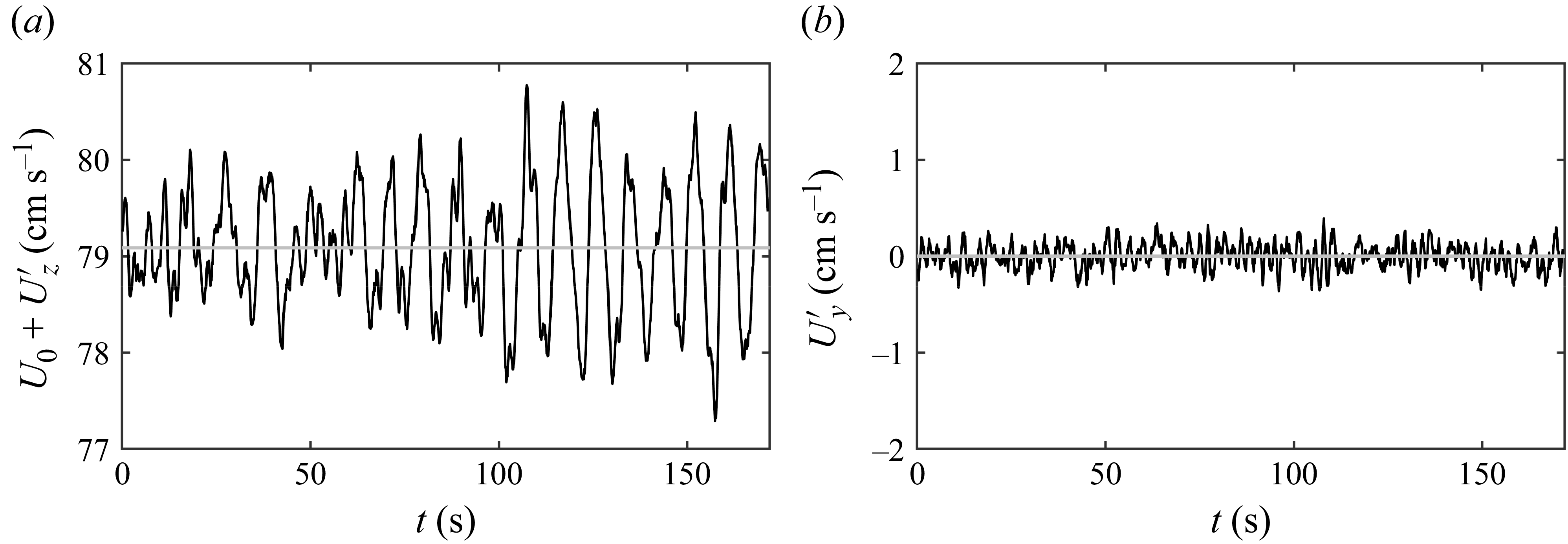
 a
a b
b y=16.2cm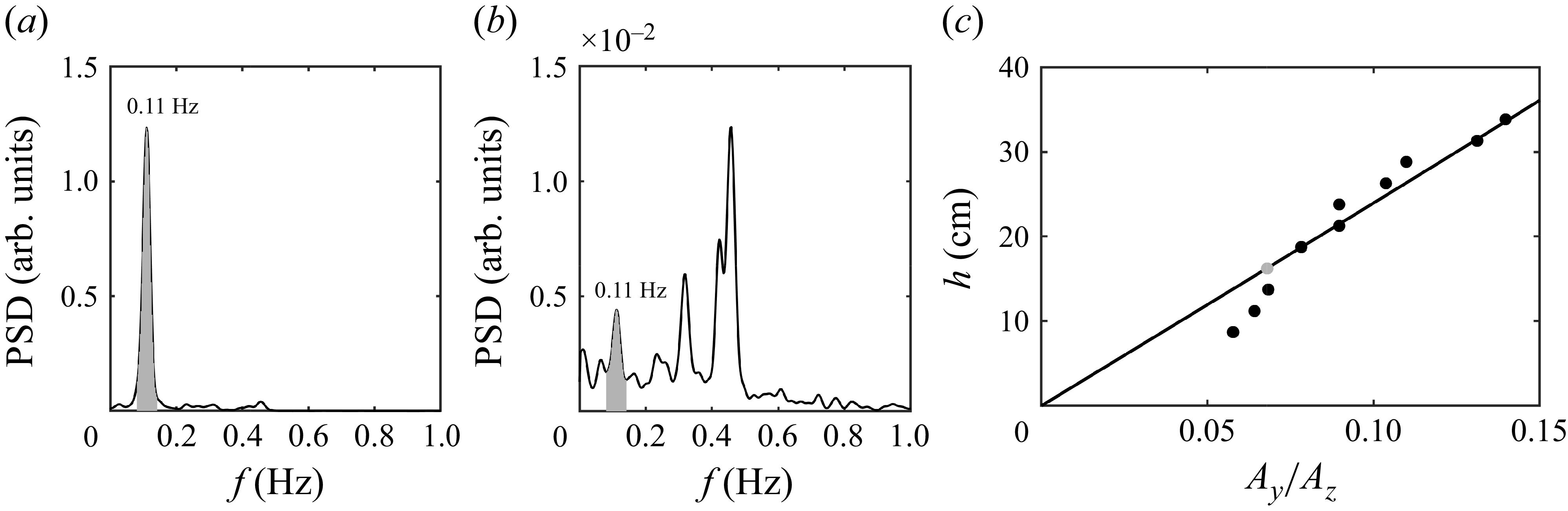
 a
a b
b c
c h
h L=7.5m
 a
a z/c=11.2
 U0
U0 z
z x
x y
y b
b eα
eα xα
xα σα
σα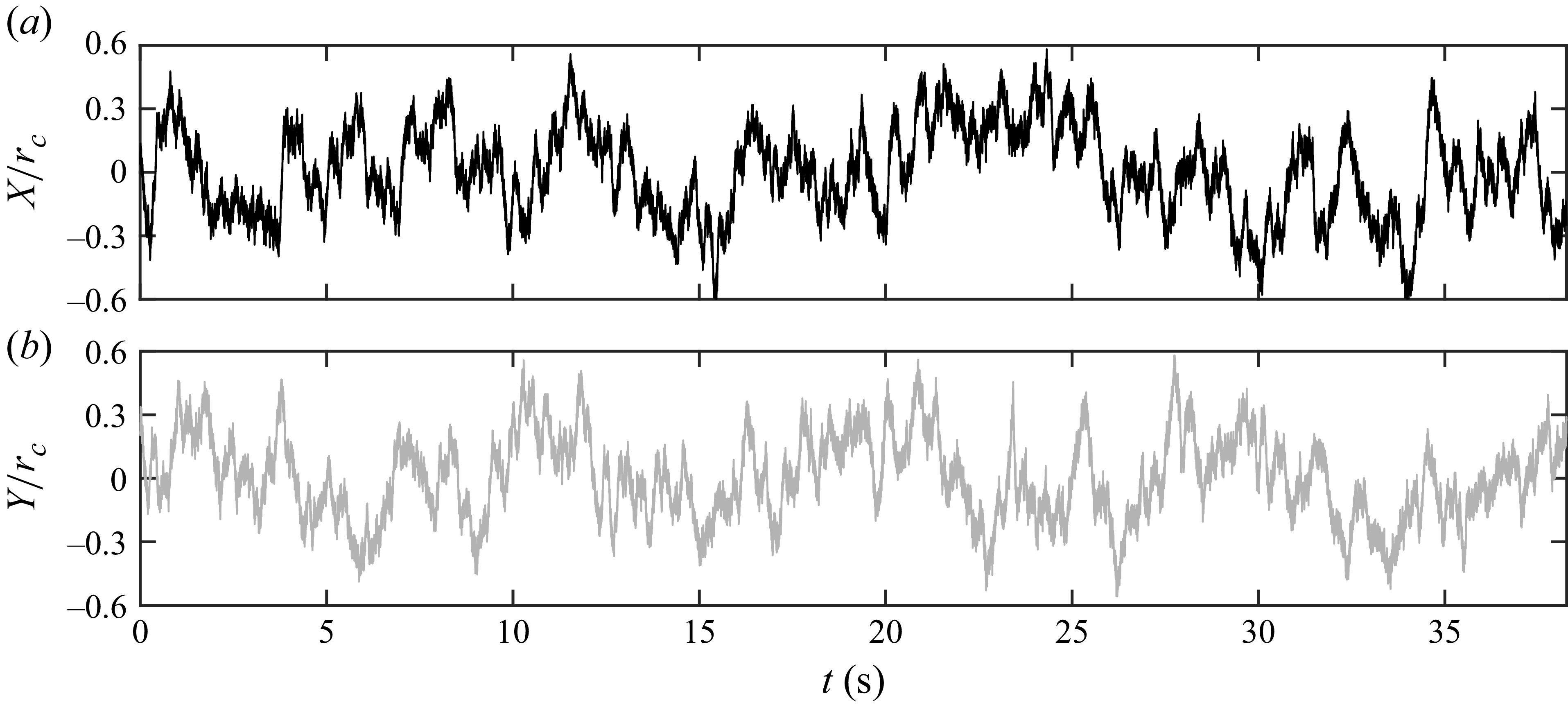
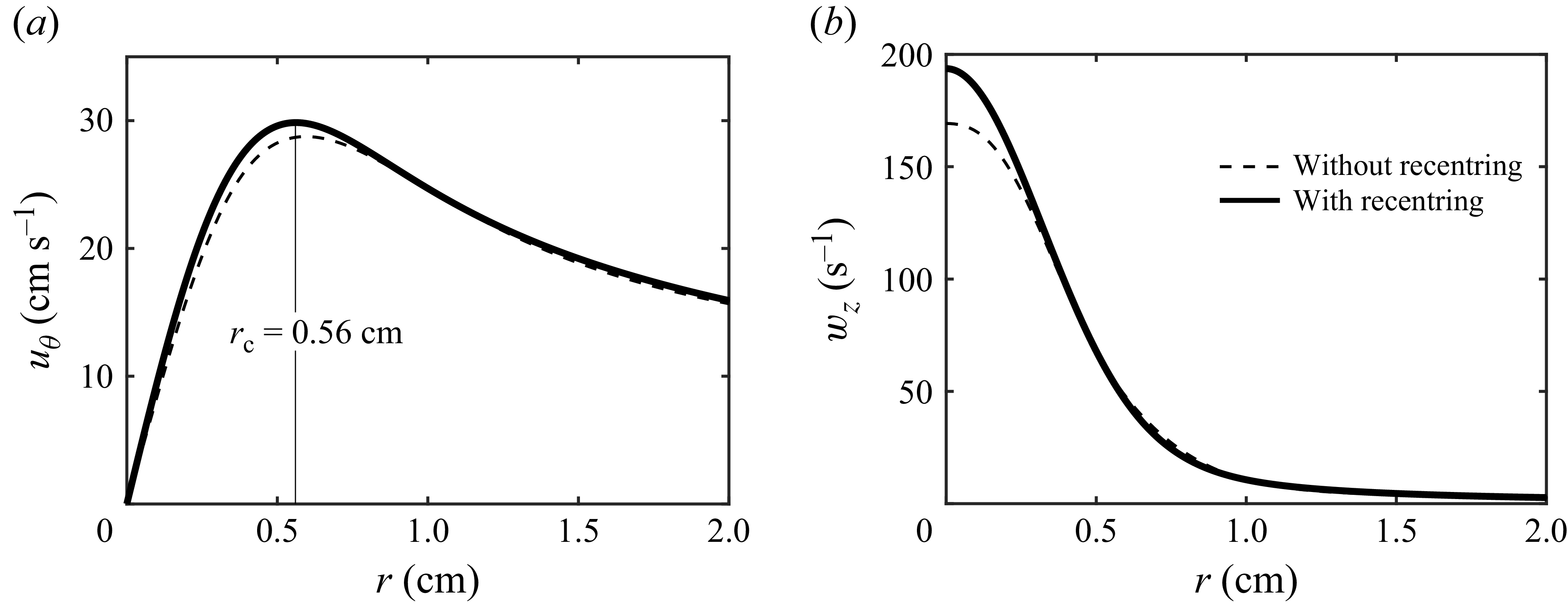
 a
a b
b z/c=11.2
 u¯θ
u¯θ w¯z
w¯z uθ
uθ wz
wz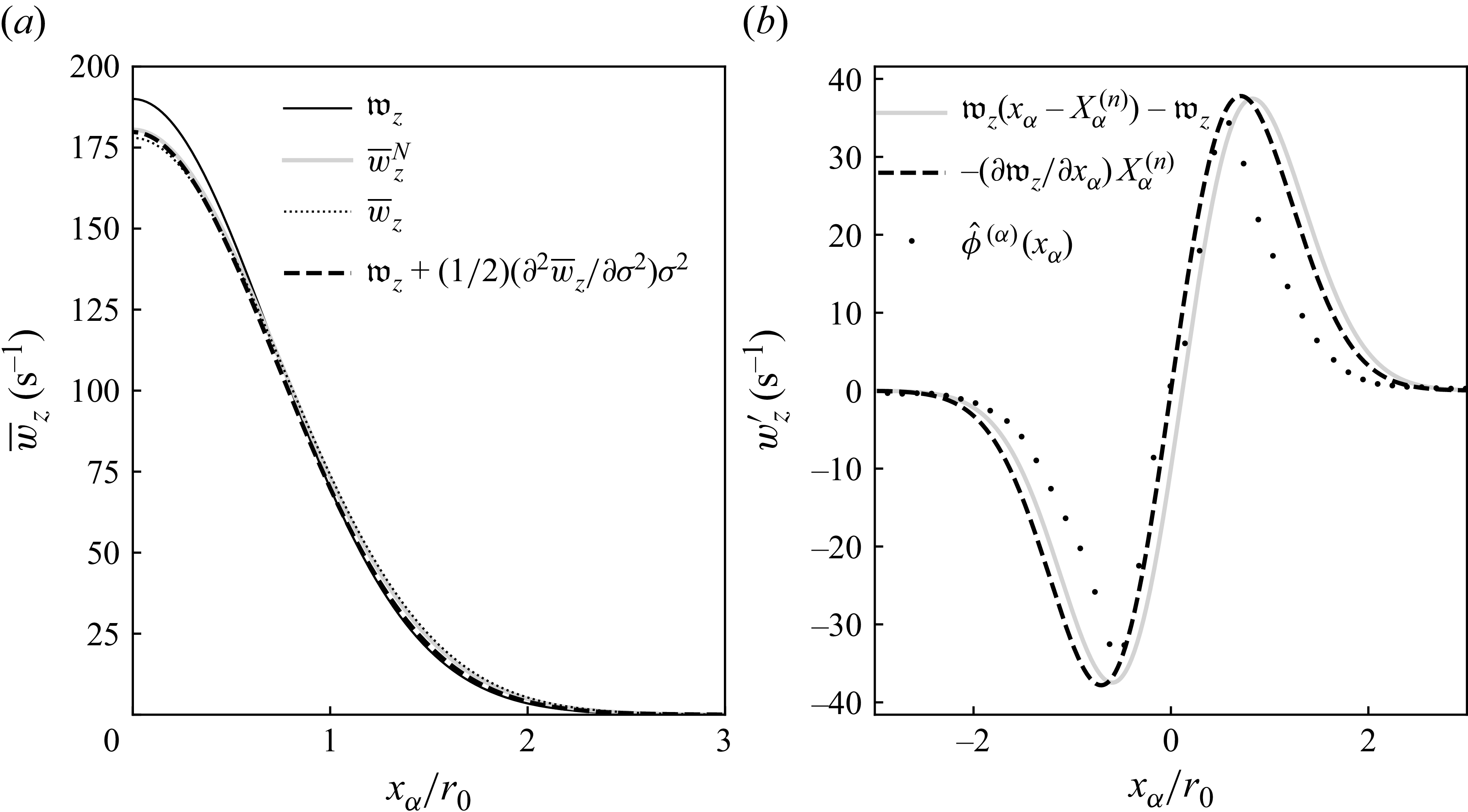
 (a)
(a) (b)
(b) Xα/rc=0.2
 ϕ^(α)
ϕ^(α) xα
xα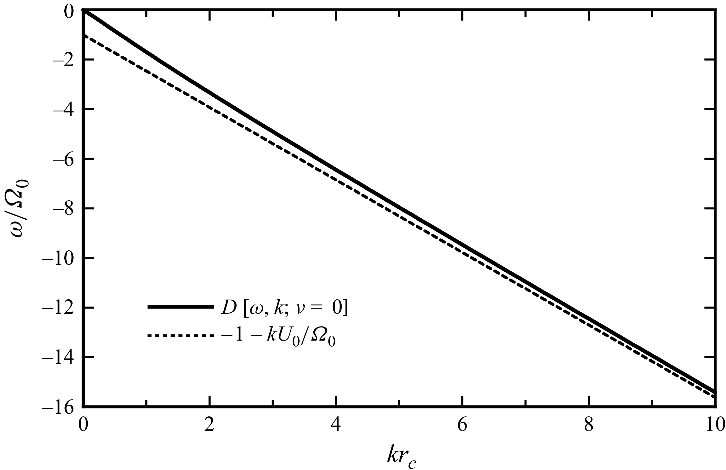
 U0
U0 ω(k)
ω(k) rc
rc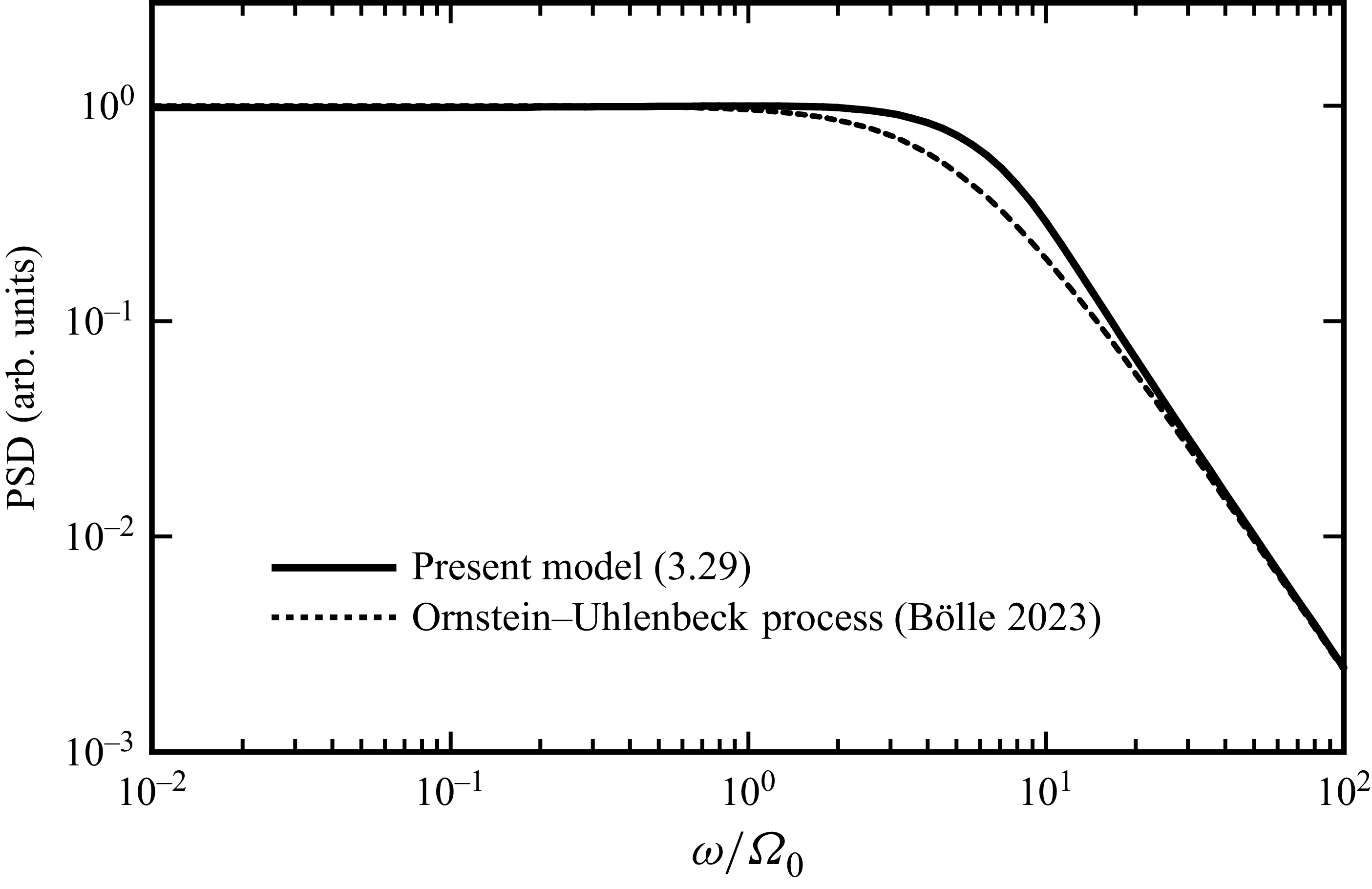
 λ
λ
 (a)
(a) (b)
(b) eα
eα σ^α
σ^α M^αα−1
 Xμ
Xμ (a)
(a) (b)
(b) M^μμ
M^μμ σ^μ
σ^μ
 x1
x1 x2
x2 (a)
(a) ψ^1(1)
 (b)
(b) ψ^2(1)
 (c)
(c) ψ^1(2)
 (d)
(d) ψ^2(2)
 eα
eα σ^α
σ^α M^αα−1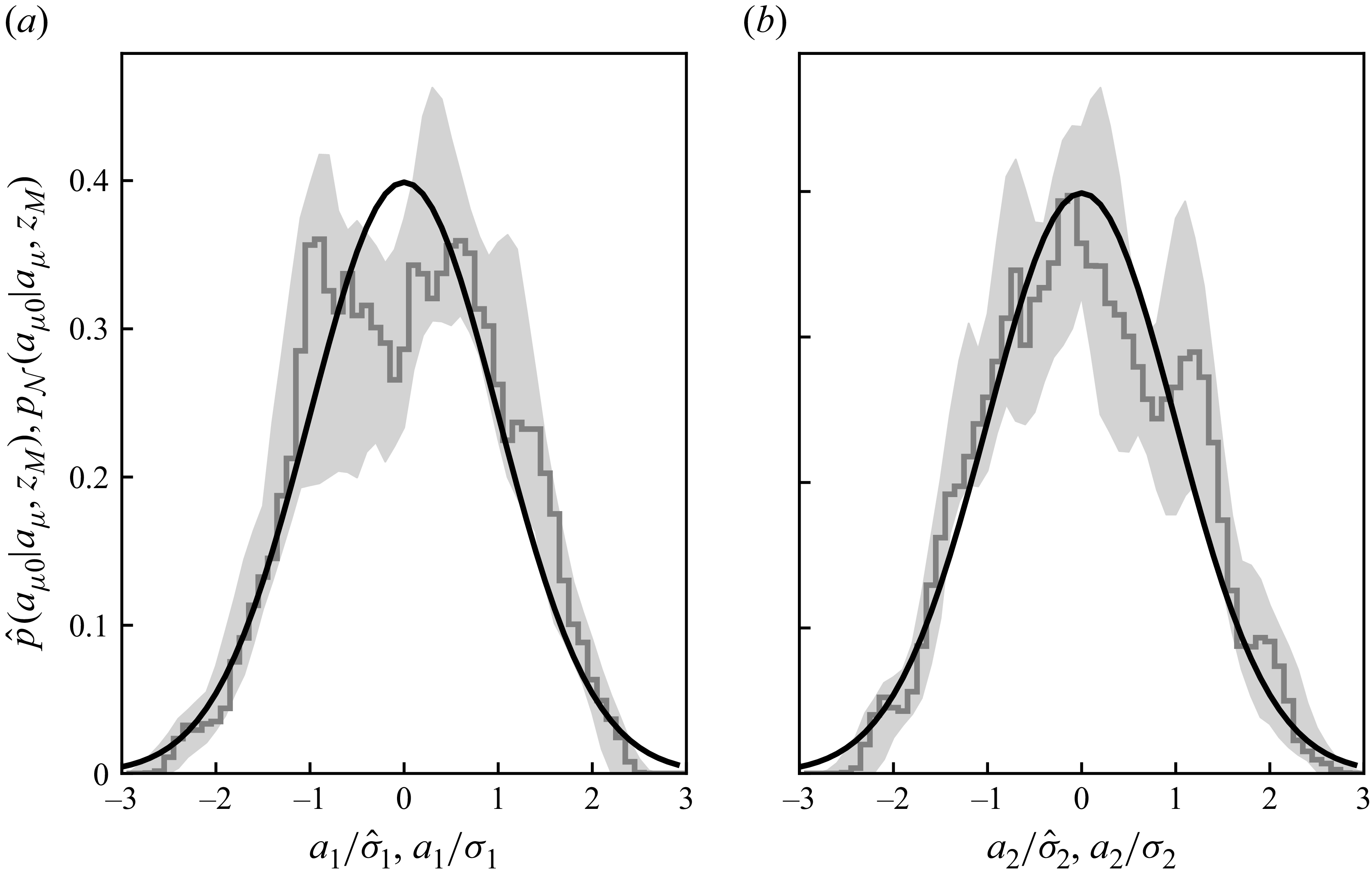
 p^(aμ0|aμ,zM)
 (a)
(a) (b)
(b) Nb=103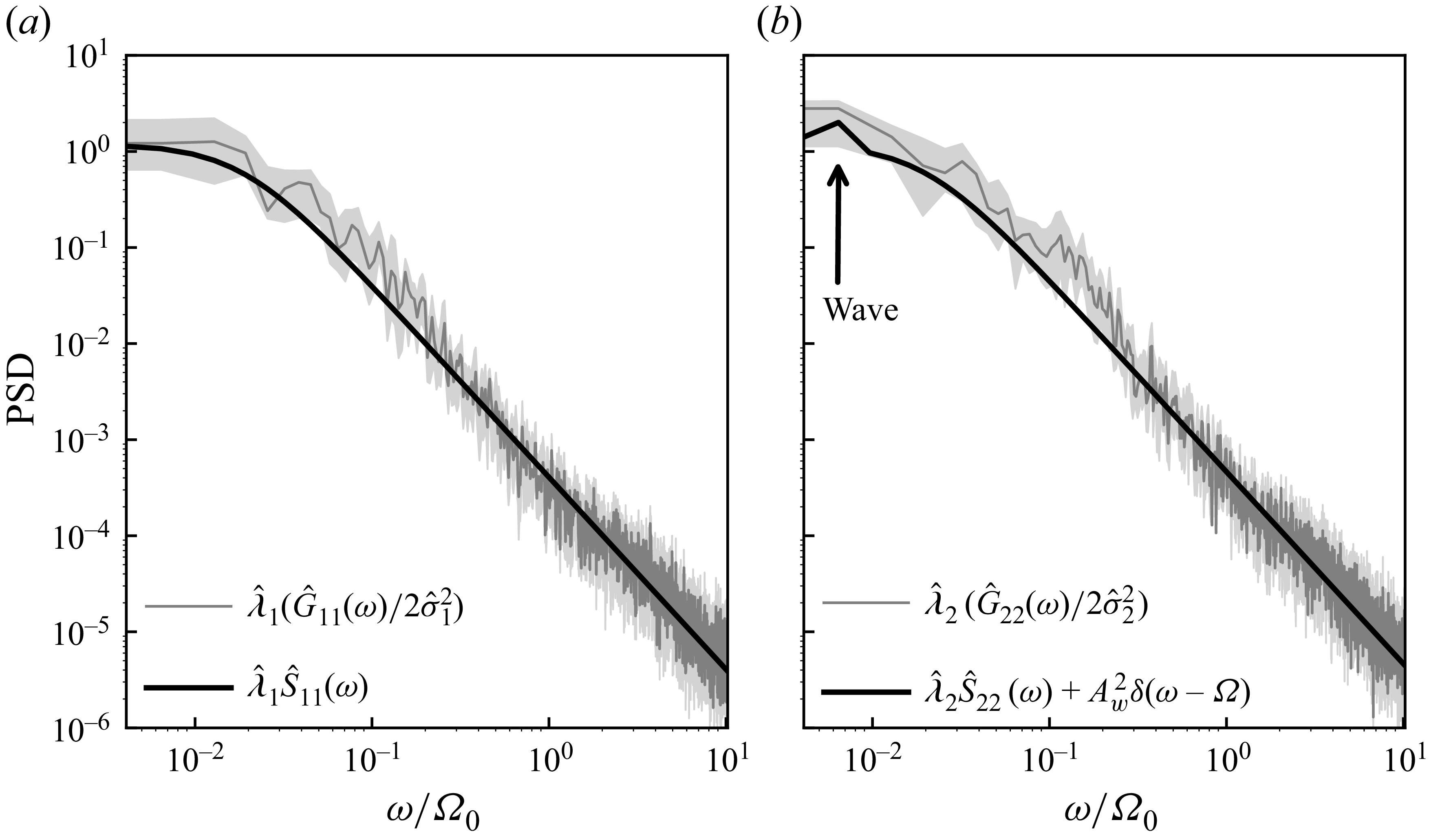
 (a)
(a) (b)
(b) Nb=103
 (b)
(b)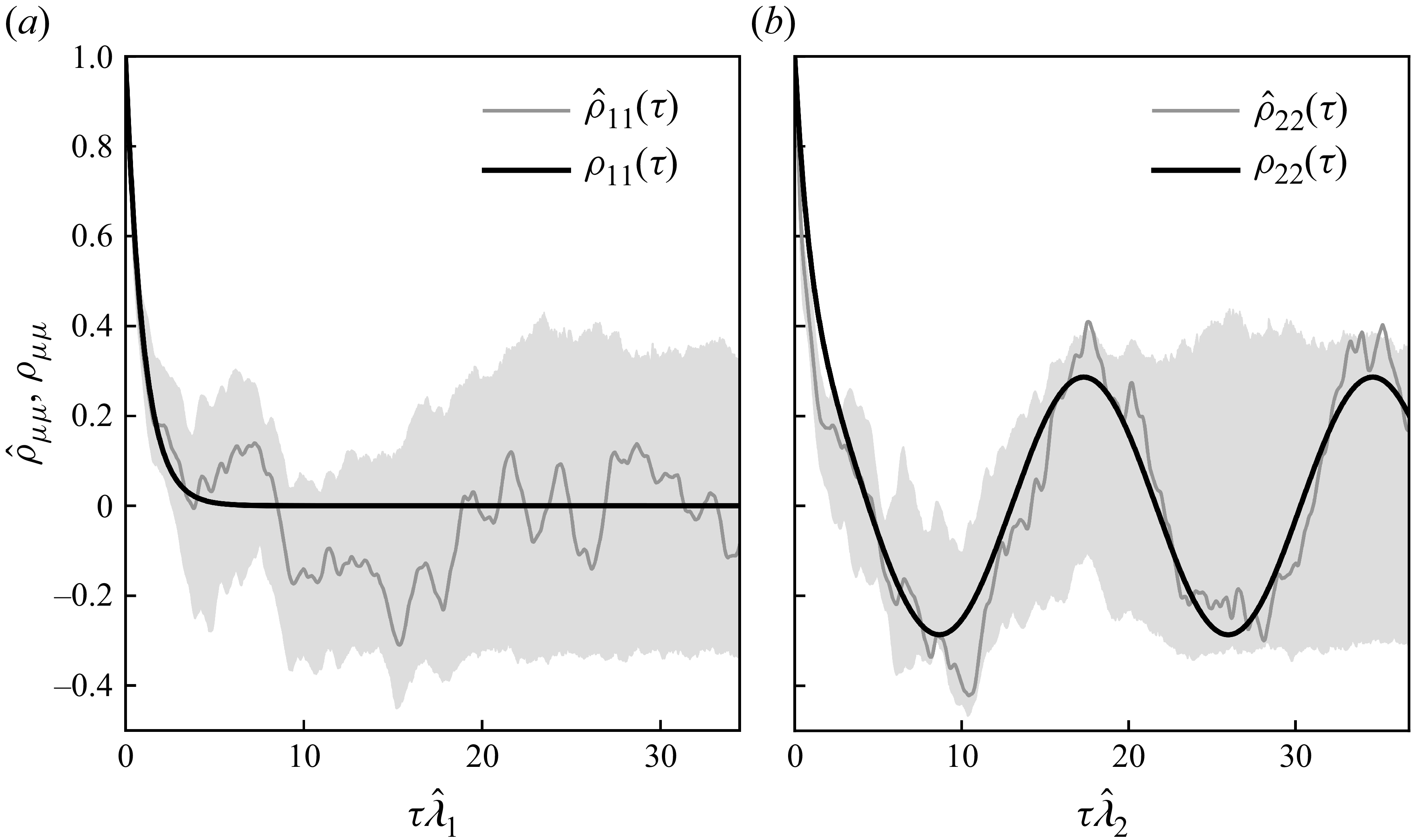
 ρμμ
ρμμ ρ^μμ
ρ^μμ (a)
(a) (b)
(b) Nb=103


 Open access

