


1. Introduction
Elastoinertial turbulence (EIT) is a chaotic state resulting from the interplay between inertia and elasticity, and is suspected to set a limit on the achievable drag reduction in turbulent flows using polymer additives (Samanta et al. Reference Samanta, Dubief, Holzner, Schäfer, Morozov, Wagner and Hof2013; Shekar et al. Reference Shekar, McMullen, Wang, McKeon and Graham2019). Direct numerical simulation (DNS) of EIT is computationally demanding due to the requirement of resolving small-scale dynamics, which is essential to sustain EIT (Sid et al. Reference Sid, Terrapon and Dubief2018). The dynamics of EIT is fundamentally two-dimensional (2-D) (Sid et al. Reference Sid, Terrapon and Dubief2018) and a 2-D numerical simulation of EIT requires $O(10^6)$
degrees of freedom (DOF), making the investigation of its dynamics challenging. A reduced-order model (ROM) of EIT having fewer DOF not only would accelerate the investigation of the dynamics of EIT but alsomay open the door to developing control strategies to suppress EIT, which would allow turbulent drag reduction beyond the maximum drag reduction (MDR) limit (Linot et al. Reference Linot, Zeng and Graham2023b
). It is also of fundamental interest for any complex flow phenomenon to know how many DOF are actually required to describe its dynamics. Specifically, we have recently shown that the dynamics of 2-D EIT in channel flow is dominated by a self-similar family of well-structured travelling waves (Kumar & Graham Reference Kumar and Graham2024), and a natural question is how many DOF are required to capture this structure.
$O(10^6)$
degrees of freedom (DOF), making the investigation of its dynamics challenging. A reduced-order model (ROM) of EIT having fewer DOF not only would accelerate the investigation of the dynamics of EIT but alsomay open the door to developing control strategies to suppress EIT, which would allow turbulent drag reduction beyond the maximum drag reduction (MDR) limit (Linot et al. Reference Linot, Zeng and Graham2023b
). It is also of fundamental interest for any complex flow phenomenon to know how many DOF are actually required to describe its dynamics. Specifically, we have recently shown that the dynamics of 2-D EIT in channel flow is dominated by a self-similar family of well-structured travelling waves (Kumar & Graham Reference Kumar and Graham2024), and a natural question is how many DOF are required to capture this structure.
In this study, we use data-driven modelling techniques for the time evolution of 2-D channel flow EIT. We begin by considering the full-state data $ \boldsymbol {q}$
, which resides in the ambient space
$ \boldsymbol {q}$
, which resides in the ambient space $ \mathbb {R}^{d_N}$
and evolves over time according to
$ \mathbb {R}^{d_N}$
and evolves over time according to ${\rm d}\boldsymbol {q}/{\rm d}t = \boldsymbol {f}(\boldsymbol {q})$
, where the mesh resolution and the number of state variables determine the size of
${\rm d}\boldsymbol {q}/{\rm d}t = \boldsymbol {f}(\boldsymbol {q})$
, where the mesh resolution and the number of state variables determine the size of $d_N$
. The foundation of the data-driven reduced-order modelling approach applied here is that the long-time dynamics of a dissipative system collapse onto a relatively low-dimensional invariant manifold (Hopf Reference Hopf1948; Foias et al. Reference Foias, Sell and Temam1988; Temam Reference Temam1989). By mapping
$d_N$
. The foundation of the data-driven reduced-order modelling approach applied here is that the long-time dynamics of a dissipative system collapse onto a relatively low-dimensional invariant manifold (Hopf Reference Hopf1948; Foias et al. Reference Foias, Sell and Temam1988; Temam Reference Temam1989). By mapping $ \boldsymbol {q}$
to invariant manifold coordinates
$ \boldsymbol {q}$
to invariant manifold coordinates $ \boldsymbol {h} \in \mathbb {R}^{d_h} (\textrm{manifold dimension}\ d_h\lt d_N)$
, we can describe the evolution of
$ \boldsymbol {h} \in \mathbb {R}^{d_h} (\textrm{manifold dimension}\ d_h\lt d_N)$
, we can describe the evolution of $ \boldsymbol {h}$
with a new equation
$ \boldsymbol {h}$
with a new equation $ {\rm d}\boldsymbol {h}/{\rm d}t = \boldsymbol {g}(\boldsymbol {h})$
in these manifold coordinates.
$ {\rm d}\boldsymbol {h}/{\rm d}t = \boldsymbol {g}(\boldsymbol {h})$
in these manifold coordinates.
A classical approach to dimension reduction is principal component analysis (PCA) (also known as proper orthogonal decomposition or POD in fluid dynamics) (Holmes et al. Reference Holmes, Lumley, Berkooz and Rowley2012). However, PCA projects data onto a flat manifold because it is an inherently linear technique, and thus may not adequately represent the generally non-flat invariant manifold where data from a complex nonlinear system lies. To capture nonlinear manifold structure, autoencoders are widely used (Kramer Reference Kramer1991; Milano & Koumoutsakos Reference Milano and Koumoutsakos2002; Linot & Graham Reference Linot and Graham2020), which is the approach we pursue here. In high-dimensional systems, it can be beneficial to first apply PCA for linear dimension reduction, followed by using an autoencoder for further reduction (Linot & Graham Reference Linot and Graham2023; Young et al. Reference Young, Corona, Datta, Helgeson and Graham2023; Constante-Amores et al. Reference Constante-Amores, Linot and Graham2024). Once a low-dimensional representation of the full system state is identified, we can proceed with data-driven modelling of the dynamics to find $\boldsymbol {g}$
. We use the framework, known as ‘neural ordinary differential equations (NODEs)’ (Chen et al. Reference Chen, Rubanova, Bettencourt, Duvenaud, Bengio, Wallach, Larochelle, Grauman, Cesa-Bianchi and Garnett2018; Linot & Graham Reference Linot and Graham2022) that represents the vector field
$\boldsymbol {g}$
. We use the framework, known as ‘neural ordinary differential equations (NODEs)’ (Chen et al. Reference Chen, Rubanova, Bettencourt, Duvenaud, Bengio, Wallach, Larochelle, Grauman, Cesa-Bianchi and Garnett2018; Linot & Graham Reference Linot and Graham2022) that represents the vector field $\boldsymbol {g}$
as a neural network. It is important to note that the Markovian nature and continuous-time framework inherent to NODEs are well-aligned with the underlying physics of the nonlinear turbulent dynamics. This framework, which we denote DManD (data-driven manifold dynamics), has been applied successfully to a wide variety of nonlinear turbulent dynamics, including Kolmogorov flow, plane Couette flow and pipe flow (Pérez-De-Jesús & Graham Reference Pérez-De-Jesús and Graham2023; Linot & Graham Reference Linot and Graham2023; Constante-Amores et al. Reference Constante-Amores, Linot and Graham2024; Constante-Amores & Graham Reference Constante-Amores and Graham2024). The DManD models have proven capable of accurately tracking short-term dynamics for at least one Lyapunov time and capturing key statistics of long-term trajectories, such as Reynolds stresses and energy balance in wall-bounded flows. Additionally, these models have been used to aid the discovery of new exact coherent structures (ECSs), where the ECSs are direct solutions of the governing equations and they have well-defined structures that organize dynamics in chaotic flows (e.g. travelling waves, periodic orbits) (Linot & Graham Reference Linot and Graham2023; Constante-Amores et al. Reference Constante-Amores, Linot and Graham2024).
$\boldsymbol {g}$
as a neural network. It is important to note that the Markovian nature and continuous-time framework inherent to NODEs are well-aligned with the underlying physics of the nonlinear turbulent dynamics. This framework, which we denote DManD (data-driven manifold dynamics), has been applied successfully to a wide variety of nonlinear turbulent dynamics, including Kolmogorov flow, plane Couette flow and pipe flow (Pérez-De-Jesús & Graham Reference Pérez-De-Jesús and Graham2023; Linot & Graham Reference Linot and Graham2023; Constante-Amores et al. Reference Constante-Amores, Linot and Graham2024; Constante-Amores & Graham Reference Constante-Amores and Graham2024). The DManD models have proven capable of accurately tracking short-term dynamics for at least one Lyapunov time and capturing key statistics of long-term trajectories, such as Reynolds stresses and energy balance in wall-bounded flows. Additionally, these models have been used to aid the discovery of new exact coherent structures (ECSs), where the ECSs are direct solutions of the governing equations and they have well-defined structures that organize dynamics in chaotic flows (e.g. travelling waves, periodic orbits) (Linot & Graham Reference Linot and Graham2023; Constante-Amores et al. Reference Constante-Amores, Linot and Graham2024).
In this study, we develop a data-driven model of EIT in 2-D channel flow. We introduce the viscoelastic data-driven manifold dynamics (VEDManD) framework, which enables the construction of low-dimensional models that faithfully capture the short-time tracking and long-time statistics in the present case using only 50 DOF (figure 1). The remainder of this article is organized as follows: § 2 outlines the methodological framework, § 3discusses the results and § 4 concludes with final remarks.
Framework of VEDManD used to develop a ROM of EIT.

2. Formulation and governing equations
2.1. Direct numerical simulation of EIT
The dimensionless momentum and incompressible mass conservation equations are
 \begin{equation} \frac {\partial \boldsymbol {u}}{\partial t}+\boldsymbol {u}\cdot \nabla \boldsymbol {u} =-\nabla p+\frac {\beta }{\textit {Re}} \nabla ^2 \boldsymbol {u} + \frac {1-\beta }{\textit {Re}} \nabla \cdot \boldsymbol {\tau }_p+f(t)\boldsymbol {e}_x,\qquad \nabla \cdot \boldsymbol {u}=0, \end{equation}
where the non-dimensional velocity and pressure fields are denoted by $\boldsymbol {u}$
and
$\boldsymbol {u}$
and $p$
, respectively. The unit vector along the streamwise direction is denoted
$p$
, respectively. The unit vector along the streamwise direction is denoted $\boldsymbol{e}_x$
. Lengths and velocities are made non-dimensional using the channel half-width (
$\boldsymbol{e}_x$
. Lengths and velocities are made non-dimensional using the channel half-width ( $H$
) and the Newtonian laminar centreline velocity (
$H$
) and the Newtonian laminar centreline velocity ( $U_c$
), respectively. The Reynolds number
$U_c$
), respectively. The Reynolds number ${\textit {Re}}=\rho U_c H/\eta$
, where
${\textit {Re}}=\rho U_c H/\eta$
, where $\rho$
and
$\rho$
and $\eta$
are fluid density and total zero-shear rate viscosity. The solvent viscosity is
$\eta$
are fluid density and total zero-shear rate viscosity. The solvent viscosity is $\eta _s$
and
$\eta _s$
and $\beta =\eta _s/\eta$
. The polymer stress tensor
$\beta =\eta _s/\eta$
. The polymer stress tensor $\boldsymbol{\tau}_p$
is modelled with the finitely extensible nonlinear elastic with Peterlin closure (FEN-P) dumbbell constitutive equation:
$\boldsymbol{\tau}_p$
is modelled with the finitely extensible nonlinear elastic with Peterlin closure (FEN-P) dumbbell constitutive equation:
 \begin{equation} \frac {\partial \boldsymbol {\alpha }}{\partial t}+\boldsymbol {u}\cdot \nabla \boldsymbol {\alpha } - \boldsymbol {\alpha }\cdot \nabla \boldsymbol {u}-(\boldsymbol {\alpha }\cdot \nabla \boldsymbol {u})^T=-\boldsymbol {\tau }_p+\frac {1}{{\textit {Re}} {\textit {Sc}}} \nabla ^2 \boldsymbol {\alpha }, \end{equation}
 \begin{equation} \boldsymbol {\tau }_p= \frac {1}{\textit {Wi}} \left ( \frac {\boldsymbol {\alpha }}{1-\mathrm {tr}(\boldsymbol {\alpha })/b}-\boldsymbol {\boldsymbol{I}}\right ), \end{equation}
where $\boldsymbol {\alpha }$
is the conformation tensor,
$\boldsymbol {\alpha }$
is the conformation tensor, $b$
is the maximum extensibility of the polymer chains and
$b$
is the maximum extensibility of the polymer chains and $\boldsymbol {\boldsymbol{I}}$
is the identity tensor. The Weissenberg number
$\boldsymbol {\boldsymbol{I}}$
is the identity tensor. The Weissenberg number $\textit {Wi}=\lambda U_c/H$
, where
$\textit {Wi}=\lambda U_c/H$
, where $\lambda$
is the polymer relaxation time. To ensure numerical stability, we include a small diffusion term in the evolution equation of the conformation tensor (2.2), whose strength is controlled by the Schmidt number
$\lambda$
is the polymer relaxation time. To ensure numerical stability, we include a small diffusion term in the evolution equation of the conformation tensor (2.2), whose strength is controlled by the Schmidt number $Sc=\eta /(\rho D)$
, where
$Sc=\eta /(\rho D)$
, where $D$
is the diffusion coefficient of the polymer molecules.
$D$
is the diffusion coefficient of the polymer molecules.
We solve the governing equations in 2-D channel flow using no-slip boundary conditions at the channel walls, $y=\pm 1$
. The introduction of diffusion requires boundary conditions for
$y=\pm 1$
. The introduction of diffusion requires boundary conditions for $\boldsymbol {\alpha }$
to evolve (2.2). As has been done elsewhere (e.g. Sid et al. Reference Sid, Terrapon and Dubief2018), at the walls, we solve (2.2) with no diffusion term (i.e.
$\boldsymbol {\alpha }$
to evolve (2.2). As has been done elsewhere (e.g. Sid et al. Reference Sid, Terrapon and Dubief2018), at the walls, we solve (2.2) with no diffusion term (i.e. $1/Sc=0$
) and use the solution as the boundary condition on
$1/Sc=0$
) and use the solution as the boundary condition on $\boldsymbol {\alpha }$
for (2.2) with finite
$\boldsymbol {\alpha }$
for (2.2) with finite $Sc$
. We impose periodic boundary conditions in the flow (
$Sc$
. We impose periodic boundary conditions in the flow ( $x$
) direction. An external force in the streamwise direction (
$x$
) direction. An external force in the streamwise direction ( $f(t)\boldsymbol {e}_x$
) drives the flow. This forcing is chosen at each time step to ensure that the volumetric flow rate remains at the Newtonian laminar value.
$f(t)\boldsymbol {e}_x$
) drives the flow. This forcing is chosen at each time step to ensure that the volumetric flow rate remains at the Newtonian laminar value.
Direct numerical simulations are performed using Dedalus (Burns et al. Reference Burns, Vasil, Oishi, Lecoanet and Brown2020), an open-source tool based on the spectral method. The channel has a length of $5$
units and a height of
$5$
units and a height of $2$
units, and the computational domain is discretized using 256 Fourier and 1024 Chebyshev basis functions with 3/2 dealiasing factor in the streamwise (
$2$
units, and the computational domain is discretized using 256 Fourier and 1024 Chebyshev basis functions with 3/2 dealiasing factor in the streamwise ( $x$
) and wall-normal (
$x$
) and wall-normal ( $y$
) directions, respectively. We consider a dilute polymer solution (
$y$
) directions, respectively. We consider a dilute polymer solution ( $\beta =0.97$
) of long polymer chains (
$\beta =0.97$
) of long polymer chains ( $b=6400$
) at
$b=6400$
) at ${\textit {Re}}=3000$
,
${\textit {Re}}=3000$
, $\textit {Wi}=35$
. For polymer additives, such as polyethylene oxide and polyacrylamide, this value of
$\textit {Wi}=35$
. For polymer additives, such as polyethylene oxide and polyacrylamide, this value of $b$
corresponds to molecular weights
$b$
corresponds to molecular weights $\sim 300$
kDa and
$\sim 300$
kDa and $\sim 500$
kDa, respectively. The Schmidt number is
$\sim 500$
kDa, respectively. The Schmidt number is $Sc=250$
, consistent with previous studies (Sid et al. Reference Sid, Terrapon and Dubief2018; Kumar & Graham Reference Kumar and Graham2024).
$Sc=250$
, consistent with previous studies (Sid et al. Reference Sid, Terrapon and Dubief2018; Kumar & Graham Reference Kumar and Graham2024).
2.2. Linear dimension reduction: viscoelastic proper orthogonal decomposition
Due to the very high dimension of the EIT data ( ${\approx}1.6 \times 10^6$
), it is desirable to begin the dimension reduction process with a linear step to reduce to a smaller (but still fairly large) dimension at which the subsequent nonlinear step will be more tractable (figure 1). To do so, we use a viscoelastic variant (Wang et al. Reference Wang, Graham, Hahn and Xi2014) of POD (Holmes et al. Reference Holmes, Lumley, Berkooz and Rowley2012), which we will denote ‘VEPOD’. The aim of VEPOD is to find a function
${\approx}1.6 \times 10^6$
), it is desirable to begin the dimension reduction process with a linear step to reduce to a smaller (but still fairly large) dimension at which the subsequent nonlinear step will be more tractable (figure 1). To do so, we use a viscoelastic variant (Wang et al. Reference Wang, Graham, Hahn and Xi2014) of POD (Holmes et al. Reference Holmes, Lumley, Berkooz and Rowley2012), which we will denote ‘VEPOD’. The aim of VEPOD is to find a function $\boldsymbol {\psi }(\boldsymbol {x})$
that maximizes the objective function
$\boldsymbol {\psi }(\boldsymbol {x})$
that maximizes the objective function
 \begin{equation} E\{ | \langle \boldsymbol {q}(\boldsymbol {x}), \boldsymbol {\psi }(\boldsymbol {x}) \rangle |^2\} \end{equation}
given the constraint $\langle \boldsymbol {\psi }(\boldsymbol {x}), \boldsymbol {\psi }(\boldsymbol {x}) \rangle =1$
, where
$\langle \boldsymbol {\psi }(\boldsymbol {x}), \boldsymbol {\psi }(\boldsymbol {x}) \rangle =1$
, where $\boldsymbol {x}$
denotes the position and
$\boldsymbol {x}$
denotes the position and $\langle \cdot , \cdot \rangle$
represents an inner product (further discussed below). The expectation and modulus operations over the ensemble of data are given by
$\langle \cdot , \cdot \rangle$
represents an inner product (further discussed below). The expectation and modulus operations over the ensemble of data are given by $E\{\cdot \}$
and
$E\{\cdot \}$
and $|\cdot |$
, respectively. Here,
$|\cdot |$
, respectively. Here, $\boldsymbol {q}(\boldsymbol {x})$
is a vector containing instantaneous state variables and the ensemble we average over is a long time series.
$\boldsymbol {q}(\boldsymbol {x})$
is a vector containing instantaneous state variables and the ensemble we average over is a long time series.
An appropriate inner product for VEPOD can be found by considering the total mechanical energy of the fluid, which consists of the kinetic energy contribution ( $U_k$
) from the velocity and the elastic energy contribution (
$U_k$
) from the velocity and the elastic energy contribution ( $U_e$
) from the stretching of the polymer chains. For the FENE-P model, precisely computing the mechanical energy is challenging because of the limitations introduced by Peterlin’s approximation. However, an approximate mechanical energy can be given as
$U_e$
) from the stretching of the polymer chains. For the FENE-P model, precisely computing the mechanical energy is challenging because of the limitations introduced by Peterlin’s approximation. However, an approximate mechanical energy can be given as
 \begin{equation} U_{tot}=U_{k}+U_{e}= \frac {1}{2} \int _{\Omega } \left \{\boldsymbol {u} \cdot \boldsymbol {u} + \frac {1-\beta }{Re Wi}\boldsymbol {\theta } : \boldsymbol {\theta }\right \} {\rm d}\boldsymbol {x}, \end{equation}
where $\boldsymbol {\theta } \cdot \boldsymbol {\theta }=\boldsymbol {\alpha }/(1-\mathrm ({tr}(\boldsymbol {\alpha })/b))$
(Wang et al. Reference Wang, Graham, Hahn and Xi2014) and
$\boldsymbol {\theta } \cdot \boldsymbol {\theta }=\boldsymbol {\alpha }/(1-\mathrm ({tr}(\boldsymbol {\alpha })/b))$
(Wang et al. Reference Wang, Graham, Hahn and Xi2014) and $\Omega$
denotes domain volume. For the Oldroyd-B model (
$\Omega$
denotes domain volume. For the Oldroyd-B model ( $b \to \infty$
), (2.5) represents the exact mechanical energy. Corresponding to this energy definition, an appropriate state variable
$b \to \infty$
), (2.5) represents the exact mechanical energy. Corresponding to this energy definition, an appropriate state variable $\boldsymbol {q}(\boldsymbol {x})$
is
$\boldsymbol {q}(\boldsymbol {x})$
is
 \begin{equation} \boldsymbol {q}=\left [\boldsymbol {u}, \boldsymbol {\boldsymbol{T}}\right ], \end{equation}
where $\boldsymbol {\boldsymbol{T}}=\sqrt {({1-\beta })/({Re Wi}})\boldsymbol {\theta }$
is the weighted symmetric square root of the conformation tensor, which we call the stretch tensor. Consequently, the inner product used in (2.4) can be defined as
$\boldsymbol {\boldsymbol{T}}=\sqrt {({1-\beta })/({Re Wi}})\boldsymbol {\theta }$
is the weighted symmetric square root of the conformation tensor, which we call the stretch tensor. Consequently, the inner product used in (2.4) can be defined as
 \begin{equation} \langle \boldsymbol {q,\psi }\rangle = \int _{\Omega } \boldsymbol {q}(\boldsymbol {x}) \cdot \boldsymbol {\psi }(\boldsymbol {x}) {\rm d}\boldsymbol {x}, \end{equation}
so that the inner product of $\boldsymbol {q}$
with itself yields
$\boldsymbol {q}$
with itself yields $2U_{tot}$
. Maximization of the objective function (2.4) gives a self-adjoint eigenvalue problem:
$2U_{tot}$
. Maximization of the objective function (2.4) gives a self-adjoint eigenvalue problem:
 \begin{equation} \int _{\Omega } E\{\boldsymbol {q}(\boldsymbol {x}) \boldsymbol {q}^*(\boldsymbol {y}) \} \boldsymbol {\psi }(\boldsymbol {y}) {\rm d}\boldsymbol {y}=\sigma \boldsymbol {\psi }(\boldsymbol {x}), \end{equation}
which leads to an infinite set of eigenmodes $\{\sigma _j, \boldsymbol {\psi }_j(\boldsymbol {x})\}$
arranged in decreasing value of the energy represented by the eigenvalue
$\{\sigma _j, \boldsymbol {\psi }_j(\boldsymbol {x})\}$
arranged in decreasing value of the energy represented by the eigenvalue $\sigma _j$
. The eigenfunctions
$\sigma _j$
. The eigenfunctions $\boldsymbol {\psi }_j(\boldsymbol {x})$
are orthonormal with the given inner product. The vector of VEPOD coefficients
$\boldsymbol {\psi }_j(\boldsymbol {x})$
are orthonormal with the given inner product. The vector of VEPOD coefficients $\boldsymbol {a}$
is given by
$\boldsymbol {a}$
is given by $a_j=\langle \boldsymbol {q}(\boldsymbol {x}), \boldsymbol {\psi }_j(\boldsymbol {x}) \rangle$
. The state variables can be reconstructed using VEPOD modes as
$a_j=\langle \boldsymbol {q}(\boldsymbol {x}), \boldsymbol {\psi }_j(\boldsymbol {x}) \rangle$
. The state variables can be reconstructed using VEPOD modes as
 \begin{equation} \tilde {\boldsymbol {q}}(\boldsymbol {x})=\sum _{j=1}^{d_a}a_j\boldsymbol {\psi }_j(\boldsymbol {x}), \end{equation}
where $d_a$
represents the number of VEPOD modes used in the reconstruction. To estimate the VEPOD of a discrete dataset, we arrange the snapshots of the flow state as
$d_a$
represents the number of VEPOD modes used in the reconstruction. To estimate the VEPOD of a discrete dataset, we arrange the snapshots of the flow state as
 \begin{equation} \boldsymbol {\boldsymbol{Q}}=[\boldsymbol {q}_1, \boldsymbol {q}_2, \ldots , \boldsymbol {q}_{N_t}], \end{equation}
where $\boldsymbol {q}_i=\boldsymbol {q}(t_i)$
and
$\boldsymbol {q}_i=\boldsymbol {q}(t_i)$
and $N_t$
represents the total number of snapshots. The eigenmodes of VEPOD can be obtained by solving the following discretized eigenvalue problem:
$N_t$
represents the total number of snapshots. The eigenmodes of VEPOD can be obtained by solving the following discretized eigenvalue problem:
 \begin{equation} \boldsymbol {\mathsf {Q}}\boldsymbol {\mathsf {Q}}^*\boldsymbol {\boldsymbol{W}}\boldsymbol {\psi }=\boldsymbol {\psi }\boldsymbol {\sigma }, \end{equation}
where $\boldsymbol {\sigma }$
is a diagonal matrix containing the eigenvalues, and
$\boldsymbol {\sigma }$
is a diagonal matrix containing the eigenvalues, and $\boldsymbol {\boldsymbol{W}}$
accounts for the numerical quadrature necessary for integration on a non-uniform grid.
$\boldsymbol {\boldsymbol{W}}$
accounts for the numerical quadrature necessary for integration on a non-uniform grid.
2.3. Non-linear dimension reduction and NODE
After projecting the data to the leading VEPOD modes, we perform a nonlinear dimension reduction with a ‘hybrid autoencoder’ (Linot & Graham Reference Linot and Graham2020) to determine the mapping into the manifold coordinates $\boldsymbol {h}=\boldsymbol {\chi }(\boldsymbol {a})$
, along with mapping back
$\boldsymbol {h}=\boldsymbol {\chi }(\boldsymbol {a})$
, along with mapping back $\tilde {\boldsymbol {a}}=\check {\boldsymbol {\chi }}(\boldsymbol {h})$
. This hybrid autoencoder uses two neural networks to learn the corrections from the leading VEPOD coefficients, as
$\tilde {\boldsymbol {a}}=\check {\boldsymbol {\chi }}(\boldsymbol {h})$
. This hybrid autoencoder uses two neural networks to learn the corrections from the leading VEPOD coefficients, as $\boldsymbol {h}=\boldsymbol {\chi }(\boldsymbol {a};\theta _{\mathcal {E}})=\boldsymbol {\boldsymbol{U}}^T_{d_h} \boldsymbol {a}+\boldsymbol {\mathcal {E}}(\boldsymbol {\boldsymbol{U}}^T_{d_a}\boldsymbol {a},\theta _{\mathcal {E}})$
, here
$\boldsymbol {h}=\boldsymbol {\chi }(\boldsymbol {a};\theta _{\mathcal {E}})=\boldsymbol {\boldsymbol{U}}^T_{d_h} \boldsymbol {a}+\boldsymbol {\mathcal {E}}(\boldsymbol {\boldsymbol{U}}^T_{d_a}\boldsymbol {a},\theta _{\mathcal {E}})$
, here $\boldsymbol {\boldsymbol{U}}_k \in \mathbb {R}^{d_N\times k}$
is a matrix whose columns are the first
$\boldsymbol {\boldsymbol{U}}_k \in \mathbb {R}^{d_N\times k}$
is a matrix whose columns are the first $k$
VEPOD eigenfunctions, and
$k$
VEPOD eigenfunctions, and $\boldsymbol {\mathcal {E}}$
is an encoding neural network having weights
$\boldsymbol {\mathcal {E}}$
is an encoding neural network having weights $\theta_{\mathcal{E}}$
. The mapping back to the full space is given by
$\theta_{\mathcal{E}}$
. The mapping back to the full space is given by $\tilde {\boldsymbol {a}}=\check {\boldsymbol {\chi }}({\boldsymbol {h};\theta _{\mathcal {E}}})=\boldsymbol {\boldsymbol{U}}_{d_a} ([\boldsymbol {h},0]^T+\boldsymbol {\mathcal {D}}(\boldsymbol {h};\theta _{\mathcal {D}}))$
, where
$\tilde {\boldsymbol {a}}=\check {\boldsymbol {\chi }}({\boldsymbol {h};\theta _{\mathcal {E}}})=\boldsymbol {\boldsymbol{U}}_{d_a} ([\boldsymbol {h},0]^T+\boldsymbol {\mathcal {D}}(\boldsymbol {h};\theta _{\mathcal {D}}))$
, where $\boldsymbol {\mathcal {D}}$
is a decoding neural network having weights
$\boldsymbol {\mathcal {D}}$
is a decoding neural network having weights $\theta_{\mathcal{D}}$
. The autoencoder minimizes the error
$\theta_{\mathcal{D}}$
. The autoencoder minimizes the error
 \begin{equation} \mathcal {L}=|| \boldsymbol {a}(t_i)-\check {\boldsymbol {\chi }}(\boldsymbol {\chi }(\boldsymbol {a}(t_i);\theta _{\mathcal {E}});\theta _{\mathcal {D}})||^2 + \kappa || \boldsymbol {\mathcal {E}}(\boldsymbol {\boldsymbol{U}}^T_{d_a}\boldsymbol {a}(t_i);\theta _{\mathcal {E}})+\boldsymbol {\mathcal {D}}_{d_h}(\boldsymbol {h}(t_i);\theta _{\mathcal {D}}) ||^2, \end{equation}
where the second term is a penalty to enhance the accurate representation of the leading $d_h$
VEPOD coefficients (Linot & Graham Reference Linot and Graham2020) (in this study,
$d_h$
VEPOD coefficients (Linot & Graham Reference Linot and Graham2020) (in this study, $\kappa =1$
).
$\kappa =1$
).
Once the low-dimensional representation of the full state is discovered, we use a ‘stabilized’ NODE to learn the dynamics in manifold coordinates, i.e. $ {\rm d}\boldsymbol {h}/{\rm d}t=\boldsymbol {g} (\boldsymbol {h})-\boldsymbol {\boldsymbol{A}}\boldsymbol {h}$
, where
$ {\rm d}\boldsymbol {h}/{\rm d}t=\boldsymbol {g} (\boldsymbol {h})-\boldsymbol {\boldsymbol{A}}\boldsymbol {h}$
, where $\boldsymbol {g}$
is a neural network, and
$\boldsymbol {g}$
is a neural network, and $\boldsymbol {\boldsymbol{A}}=\gamma \boldsymbol {\mathsf {I}} S(\boldsymbol {h})$
is a diagonal matrix, where
$\boldsymbol {\boldsymbol{A}}=\gamma \boldsymbol {\mathsf {I}} S(\boldsymbol {h})$
is a diagonal matrix, where $S(\boldsymbol {h})$
is the standard deviation of
$S(\boldsymbol {h})$
is the standard deviation of $\boldsymbol {h}$
and
$\boldsymbol {h}$
and $\gamma$
is a tuneable parameter. This term stabilizes the system by preventing the dynamics from drifting away from the attractor (Linot et al. Reference Linot, Burby, Tang, Balaprakash, Graham and Maulik2023a
). The NODE is trained to minimize the difference between the true state
$\gamma$
is a tuneable parameter. This term stabilizes the system by preventing the dynamics from drifting away from the attractor (Linot et al. Reference Linot, Burby, Tang, Balaprakash, Graham and Maulik2023a
). The NODE is trained to minimize the difference between the true state $\boldsymbol {h}(t_i+\Delta t_s)$
and the predicted state
$\boldsymbol {h}(t_i+\Delta t_s)$
and the predicted state $\tilde {\boldsymbol {h}}(t_i+\Delta t_s)$
:
$\tilde {\boldsymbol {h}}(t_i+\Delta t_s)$
:
 \begin{equation} \mathcal {J}=||\boldsymbol {\tilde {h}}(t_i+\Delta t_s)-\boldsymbol {h}(t_i+\Delta t_s)||^2, \end{equation}
where $\boldsymbol {\tilde {h}}(t_i+\Delta t_s)=\boldsymbol {h}(t_i)+\int _{t_i}^{t_i+\Delta t_s} (\boldsymbol {g} (\boldsymbol {h}) - \boldsymbol {\boldsymbol{A}}\boldsymbol {h} ){\rm d}t$
is a time forward prediction of the NODE over time interval
$\boldsymbol {\tilde {h}}(t_i+\Delta t_s)=\boldsymbol {h}(t_i)+\int _{t_i}^{t_i+\Delta t_s} (\boldsymbol {g} (\boldsymbol {h}) - \boldsymbol {\boldsymbol{A}}\boldsymbol {h} ){\rm d}t$
is a time forward prediction of the NODE over time interval $\Delta t_s$
. Details of the different neural networks are summarized in table 1.
$\Delta t_s$
. Details of the different neural networks are summarized in table 1.
Details of different neural networks used in the VEDManD framework. ‘Architecture’ represents the dimension of each layer and ‘Activation’ refers to the types of activation functions used, where ‘ReLU’, ‘Sig’ and ‘Lin’ stand for Rectified Linear Unit, Sigmoid and Linear activation functions, respectively. ‘Learning Rate’ represents the learning rates used during training.

The ROM of EIT in the present study has been developed using a statistically stationary dataset consisting of $1000$
time units simulated using time step
$1000$
time units simulated using time step $\Delta t=0.001$
and sampled at the interval of
$\Delta t=0.001$
and sampled at the interval of $\Delta t_s=0.025$
time units, which leads to a total of
$\Delta t_s=0.025$
time units, which leads to a total of $40\,000$
snapshots. The correlation time of the dynamics of EIT is small (
$40\,000$
snapshots. The correlation time of the dynamics of EIT is small ( ${\lt } 1$
time unit), so this dataset is sufficient to develop our ROM. Here,
${\lt } 1$
time unit), so this dataset is sufficient to develop our ROM. Here, $80\,\%$
of data have been used for training and
$80\,\%$
of data have been used for training and $20\,\%$
data for testing. The losses used to train the neural networks (2.12) and (2.13) are the ensemble-averaged over the training data. The DNS was performed in parallel mode on 24 processors on a high-performance computing (HPC) cluster and it took
$20\,\%$
data for testing. The losses used to train the neural networks (2.12) and (2.13) are the ensemble-averaged over the training data. The DNS was performed in parallel mode on 24 processors on a high-performance computing (HPC) cluster and it took ${\approx} 2$
weeks to compute for
${\approx} 2$
weeks to compute for $1000$
time units. The VEDManD framework consists of three steps, and a single processor was used to develop our ROM. The first step, the projection of the dataset on
$1000$
time units. The VEDManD framework consists of three steps, and a single processor was used to develop our ROM. The first step, the projection of the dataset on $4000$
VEPOD modes, takes
$4000$
VEPOD modes, takes ${\approx} 4$
hours. The second step, the training of the autoencoder, takes
${\approx} 4$
hours. The second step, the training of the autoencoder, takes ${\approx} 2$
days. The third step, the training of the NODE, takes
${\approx} 2$
days. The third step, the training of the NODE, takes $2{-}3$
hours. Thus, the development of ROM takes
$2{-}3$
hours. Thus, the development of ROM takes ${\approx} 2.5$
days on a single processor. Once the model is developed, it evolves dynamics for
${\approx} 2.5$
days on a single processor. Once the model is developed, it evolves dynamics for $1000$
time units in seconds on a single processor.
$1000$
time units in seconds on a single processor.
3. Results and discussion
3.1. Dimension reduction of EIT
For statistically stationary dynamics, the instantaneous state variables can be written as $\boldsymbol {u}=\overline {\boldsymbol {u}}+\boldsymbol {u}^{\prime }$
and
$\boldsymbol {u}=\overline {\boldsymbol {u}}+\boldsymbol {u}^{\prime }$
and $\boldsymbol {\mathsf {T}}=\overline {\boldsymbol {\mathsf {T}}}+\boldsymbol {\mathsf {T}}^{\prime }$
, where
$\boldsymbol {\mathsf {T}}=\overline {\boldsymbol {\mathsf {T}}}+\boldsymbol {\mathsf {T}}^{\prime }$
, where $\overline {(\cdot )}$
and
$\overline {(\cdot )}$
and $(\cdot )^{\prime }$
are the temporal mean and perturbation, respectively. Mean profiles and laminar profiles are shown in figures 2(
$(\cdot )^{\prime }$
are the temporal mean and perturbation, respectively. Mean profiles and laminar profiles are shown in figures 2( $a$
) and 2(
$a$
) and 2( $b$
), respectively. Here, we develop a ROM to capture the perturbations of the state variables:
$b$
), respectively. Here, we develop a ROM to capture the perturbations of the state variables: $\boldsymbol {q}=[\boldsymbol {u}',\boldsymbol {\mathsf {T}}']$
.
$\boldsymbol {q}=[\boldsymbol {u}',\boldsymbol {\mathsf {T}}']$
.
Mean profiles (solid lines) of the components of ( $a$
) velocity and (
$a$
) velocity and ( $b$
) stretch tensor in EIT at
$b$
) stretch tensor in EIT at ${\textit {Re}} =3000$
and
${\textit {Re}} =3000$
and $\textit {Wi}=35$
. The dotted lines show the laminar profiles at the same parameter. The temporal mean profiles of velocity in EIT are close to the laminar profiles as velocity fluctuations in EIT are weak (Sid et al. Reference Sid, Terrapon and Dubief2018).
$\textit {Wi}=35$
. The dotted lines show the laminar profiles at the same parameter. The temporal mean profiles of velocity in EIT are close to the laminar profiles as velocity fluctuations in EIT are weak (Sid et al. Reference Sid, Terrapon and Dubief2018).

The VEPOD eigenvalue spectrum of the perturbations in state variables, figure 3( $a$
), shows that the energy content of higher VEPOD modes decreases approximately exponentially for index
$a$
), shows that the energy content of higher VEPOD modes decreases approximately exponentially for index $j\gtrsim 1500$
. We find that reconstruction of the flow state using
$j\gtrsim 1500$
. We find that reconstruction of the flow state using $d_a=4000$
VEPOD modes captures
$d_a=4000$
VEPOD modes captures ${\approx} 99.8\,\%$
of the total mechanical energy and yields an accurate representation. Therefore, to develop our model we retain
${\approx} 99.8\,\%$
of the total mechanical energy and yields an accurate representation. Therefore, to develop our model we retain $4000$
VEPOD modes. We also visualize the leading VEPOD mode structure for
$4000$
VEPOD modes. We also visualize the leading VEPOD mode structure for $u_y'$
and
$u_y'$
and $T_{xx}^{\prime }$
(figure 3
c,d) and find that they resemble the most dominant travelling wave underlying EIT (Kumar & Graham Reference Kumar and Graham2024).
$T_{xx}^{\prime }$
(figure 3
c,d) and find that they resemble the most dominant travelling wave underlying EIT (Kumar & Graham Reference Kumar and Graham2024).
( $a$
) The VEPOD eigenvalue spectrum. (
$a$
) The VEPOD eigenvalue spectrum. ( $b$
) Normalized reconstruction error on the test dataset for various latent dimensions of VEPOD and autoencoder. Leading VEPOD mode structure for (
$b$
) Normalized reconstruction error on the test dataset for various latent dimensions of VEPOD and autoencoder. Leading VEPOD mode structure for ( $c$
)
$c$
) $u'_y$
and (
$u'_y$
and ( $d$
)
$d$
) $T_{xx}'$
.
$T_{xx}'$
.

Before training the neural networks, we first centre and scale the dataset by subtracting the mean and then normalizing it with the maximum standard deviation. To find a low-dimensional representation of the system, we train multiple autoencoders with varying numbers of latent dimensions and visualize the reconstruction error of VEPOD coefficients on the test dataset (figure 3 $b$
). The reconstruction error initially decreases rapidly at low
$b$
). The reconstruction error initially decreases rapidly at low $d_h$
, then shows only a marginal improvement in the reconstruction for latent dimension
$d_h$
, then shows only a marginal improvement in the reconstruction for latent dimension $d_h\gt 30$
. The VEDManD model with
$d_h\gt 30$
. The VEDManD model with $d_h=30$
struggles to quantitatively capture the dynamics, so we do not report results for it and we use the latent dimension of the autoencoder
$d_h=30$
struggles to quantitatively capture the dynamics, so we do not report results for it and we use the latent dimension of the autoencoder $d_h=50$
in the present study. To illustrate the accuracy of the reconstruction, we compare results for
$d_h=50$
in the present study. To illustrate the accuracy of the reconstruction, we compare results for $u_y'$
and
$u_y'$
and $T_{xx}^{\prime }$
fields using the autoencoder at
$T_{xx}^{\prime }$
fields using the autoencoder at $d_h=50$
(figure 4
c,d) with the corresponding DNS results (figure 4
a,b). The autoencoder faithfully reconstructs the flow state obtained from the DNS. Visual inspection of the autoencoder reconstruction reveals a very close resemblance, while a quantitative comparison between DNS and autoencoder results demonstrates differences at fine scales in the reconstruction (
$d_h=50$
(figure 4
c,d) with the corresponding DNS results (figure 4
a,b). The autoencoder faithfully reconstructs the flow state obtained from the DNS. Visual inspection of the autoencoder reconstruction reveals a very close resemblance, while a quantitative comparison between DNS and autoencoder results demonstrates differences at fine scales in the reconstruction ( ${\sim}10\,\%$
for the worst-case scenario and are confined only in a tiny region), resulting from the cumulative effects of VEPOD truncation and autoencoder reconstruction (figure 4
e,f). Further analysis shows that the error is dominated by VEPOD truncation to 4000 modes – the autoencoder error is very small. The other components exhibit similar degrees of accuracy.
${\sim}10\,\%$
for the worst-case scenario and are confined only in a tiny region), resulting from the cumulative effects of VEPOD truncation and autoencoder reconstruction (figure 4
e,f). Further analysis shows that the error is dominated by VEPOD truncation to 4000 modes – the autoencoder error is very small. The other components exhibit similar degrees of accuracy.
Instantaneous (a,c) $u'_y$
and (b,d)
$u'_y$
and (b,d) $T_{xx}'$
obtained from (a,b) DNS and (c,d) reconstruction with an autoencoder with
$T_{xx}'$
obtained from (a,b) DNS and (c,d) reconstruction with an autoencoder with $d_h=50$
. (e,f) Difference between DNS and autoencoder reconstruction normalized with the maximum values of respective fields.
$d_h=50$
. (e,f) Difference between DNS and autoencoder reconstruction normalized with the maximum values of respective fields.

( $a$
) Temporal autocorrelation of the VEPOD coefficients. (
$a$
) Temporal autocorrelation of the VEPOD coefficients. ( $b$
) First several VEPOD coefficients up to
$b$
) First several VEPOD coefficients up to $t/t_c=4$
obtained using DNS and VEDManD with
$t/t_c=4$
obtained using DNS and VEDManD with $d_h =50$
for two arbitrary initial conditions (IC
$d_h =50$
for two arbitrary initial conditions (IC $_1$
and IC
$_1$
and IC $_2$
). (
$_2$
). ( $c$
) Ensemble-averaged relative error between the VEPOD coefficients obtained using DNS and VEDManD.
$c$
) Ensemble-averaged relative error between the VEPOD coefficients obtained using DNS and VEDManD.

3.2. Low-dimensional dynamic model
Once the autoencoder maps the system on a low-dimensional representation, we train the NODE to predict dynamics. We start the presentation of the NODE results with short-time tracking. It is expected that the VEDManD predictions should closely follow DNS trajectories over a short time period before the dynamics diverges due to the chaotic nature of the system. To estimate the correlation time of the dynamics, we defined a temporal autocorrelation function ( $C(t)$
) for the VEPOD coefficients as
$C(t)$
) for the VEPOD coefficients as $C(t)=\bigg({\langle \boldsymbol {R}(\tau ) \cdot \boldsymbol {R}(\tau +t)\rangle }\bigg)/\bigg({\langle \boldsymbol {R}(\tau ) \cdot \boldsymbol {R}(\tau )\rangle }\bigg ),$
where
$C(t)=\bigg({\langle \boldsymbol {R}(\tau ) \cdot \boldsymbol {R}(\tau +t)\rangle }\bigg)/\bigg({\langle \boldsymbol {R}(\tau ) \cdot \boldsymbol {R}(\tau )\rangle }\bigg ),$
where $\langle \cdot \rangle$
represents ensemble average. Here, the parameter
$\langle \cdot \rangle$
represents ensemble average. Here, the parameter $\boldsymbol {R}$
stands for
$\boldsymbol {R}$
stands for $\boldsymbol {a}$
and
$\boldsymbol {a}$
and $\tilde {\boldsymbol {a}}$
for DNS and VEDManD, respectively. The autocorrelation functions from DNS and VEDManD are plotted in figure 5(
$\tilde {\boldsymbol {a}}$
for DNS and VEDManD, respectively. The autocorrelation functions from DNS and VEDManD are plotted in figure 5( $a$
). The correlation time of the dynamics is defined as
$a$
). The correlation time of the dynamics is defined as $t_c=\int _0^{t_z}C(t) {\rm d}t$
, where
$t_c=\int _0^{t_z}C(t) {\rm d}t$
, where $t_z$
represents the first zero of the autocorrelation function. The computed values using DNS and VEDManD are
$t_z$
represents the first zero of the autocorrelation function. The computed values using DNS and VEDManD are $t_c=0.67$
and
$t_c=0.67$
and $t_c=0.68$
, respectively, very close to each other. This time scale indicates when trajectories starting from different initial conditions or with slightly different evolution equations should start to diverge from one another. In figure 5(
$t_c=0.68$
, respectively, very close to each other. This time scale indicates when trajectories starting from different initial conditions or with slightly different evolution equations should start to diverge from one another. In figure 5( $b$
), we show the time evolution of the first several VEPOD coefficients for different initial conditions on the attractor using the VEDManD model and DNS. For
$b$
), we show the time evolution of the first several VEPOD coefficients for different initial conditions on the attractor using the VEDManD model and DNS. For $t\lt t_c$
, the model accurately predicts the EIT trajectory, deviating at longer times. In figure 6, we compare snapshots of the state obtained from the model against DNS with the same initial condition and see that for
$t\lt t_c$
, the model accurately predicts the EIT trajectory, deviating at longer times. In figure 6, we compare snapshots of the state obtained from the model against DNS with the same initial condition and see that for $t\lt t_c$
the results are very close. To quantify the deviation of the VEDManD prediction of trajectories from the DNS results, we show in figure 5(
$t\lt t_c$
the results are very close. To quantify the deviation of the VEDManD prediction of trajectories from the DNS results, we show in figure 5( $c$
) the ensemble average of the relative error of the VEPOD coefficients from VEDManD and DNS calculated over many initial conditions. The difference between the model prediction and the DNS result is small at short times, increasing on the time scale
$c$
) the ensemble average of the relative error of the VEPOD coefficients from VEDManD and DNS calculated over many initial conditions. The difference between the model prediction and the DNS result is small at short times, increasing on the time scale $t_c$
before saturating. In summary, the VEDManD model with
$t_c$
before saturating. In summary, the VEDManD model with $d_h=50$
is capable of accurately capturing the dynamics of 2-D EIT over time scales comparable to the flow correlation time.
$d_h=50$
is capable of accurately capturing the dynamics of 2-D EIT over time scales comparable to the flow correlation time.
Time series of $u_y^{\prime }$
obtained using (a−d) DNS and (e−h) VEDManD for IC
$u_y^{\prime }$
obtained using (a−d) DNS and (e−h) VEDManD for IC $_1$
in figure 5(
$_1$
in figure 5( $b$
).
$b$
).

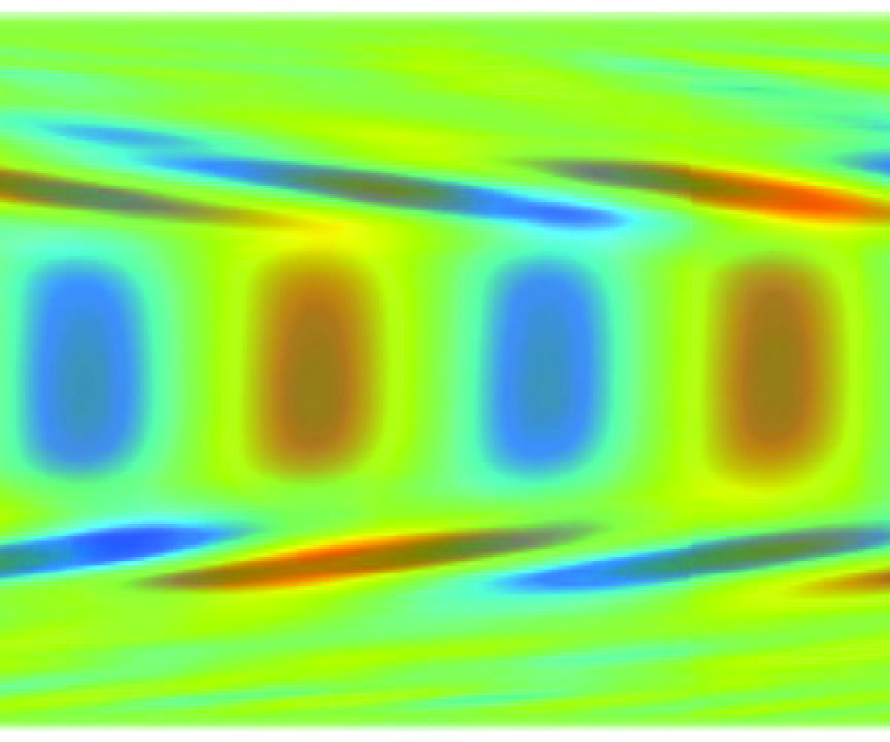
We now turn to the long-time statistics of the timeevolution, focusing on the spectral proper orthogonal decomposition (SPOD) (Towne et al. Reference Towne, Schmidt and Colonius2018), of the flow and stretch fields. In short, SPOD is a temporal variant of POD that seeks the frequency-by-frequency POD of a Fourier-transformed time-dependent flow, yielding for every frequency $f$
a spectrum of energies and modes. For a detailed description of SPOD in the context of EIT, see Kumar & Graham (Reference Kumar and Graham2024), where we used SPOD to show that the dynamics of 2-D EIT in the parameter regime examined are dominated by a family of self-similar, nested travelling waves. Here, we report the SPOD spectrum of
$f$
a spectrum of energies and modes. For a detailed description of SPOD in the context of EIT, see Kumar & Graham (Reference Kumar and Graham2024), where we used SPOD to show that the dynamics of 2-D EIT in the parameter regime examined are dominated by a family of self-similar, nested travelling waves. Here, we report the SPOD spectrum of $u_y^{\prime }$
, as this component gives the cleanest spectrum. The SPOD energy spectra of
$u_y^{\prime }$
, as this component gives the cleanest spectrum. The SPOD energy spectra of $u_y^{\prime }$
obtained from DNS and VEDManD are shown in figures 7(
$u_y^{\prime }$
obtained from DNS and VEDManD are shown in figures 7( $a$
) and 7(
$a$
) and 7( $b$
), respectively. The leading modes of both spectra contain most of the energy and exhibit peaks at the same frequencies, at least to the two significant digits (red symbols) which is the frequency resolution in the present study. We visualize the SPOD mode structures corresponding to the peaks in the SPOD spectra in figure 8. The structures obtained from the VEDManD model closely resemble the structures of travelling modes obtained from the DNS. (The mode structures are travelling waves, therefore we align their spatial phases to make comparison easier.) The precise prediction of wavenumbers and frequencies of different mode structures by the VEDManD model gives an accurate prediction of their wave speeds. Thus, we have found a highly accurate representation of EIT with
$b$
), respectively. The leading modes of both spectra contain most of the energy and exhibit peaks at the same frequencies, at least to the two significant digits (red symbols) which is the frequency resolution in the present study. We visualize the SPOD mode structures corresponding to the peaks in the SPOD spectra in figure 8. The structures obtained from the VEDManD model closely resemble the structures of travelling modes obtained from the DNS. (The mode structures are travelling waves, therefore we align their spatial phases to make comparison easier.) The precise prediction of wavenumbers and frequencies of different mode structures by the VEDManD model gives an accurate prediction of their wave speeds. Thus, we have found a highly accurate representation of EIT with $O(10)$
dimensions commencing from an initial state dimension of
$O(10)$
dimensions commencing from an initial state dimension of $O(10^6)$
. This dimension might not be the true dimension of the invariant manifold where the dynamics lives (this quantity remains difficult to estimate precisely from data for complex chaotic systems), but it is capable of providing models that faithfully capture the short-time dynamics and long-time statistics of EIT.
$O(10^6)$
. This dimension might not be the true dimension of the invariant manifold where the dynamics lives (this quantity remains difficult to estimate precisely from data for complex chaotic systems), but it is capable of providing models that faithfully capture the short-time dynamics and long-time statistics of EIT.
The SPOD eigenvalue spectra of $u_y^{\prime }$
obtained using (
$u_y^{\prime }$
obtained using ( $a$
) DNS and (
$a$
) DNS and ( $b$
) VEDManD. Red symbols indicate peaks in the leading mode of the spectra.
$b$
) VEDManD. Red symbols indicate peaks in the leading mode of the spectra.

The SPOD mode structures of (a−j) $u_y^{\prime }$
and (
$u_y^{\prime }$
and ( $k-t$
)
$k-t$
) $T_{xx}^{\prime }$
from (a−e, k−o) DNS and (f−j, p−t) VEDManD at the frequencies indicated with red symbols in figure 7.
$T_{xx}^{\prime }$
from (a−e, k−o) DNS and (f−j, p−t) VEDManD at the frequencies indicated with red symbols in figure 7.

4. Conclusion
Numerical simulations of EIT are computationally expensive due to the high number of DOF ( $O(10^6)$
) required to resolve all spatial and temporal scales. In the present study, we use data-driven methods to develop a ROM that has far fewer DOF (
$O(10^6)$
) required to resolve all spatial and temporal scales. In the present study, we use data-driven methods to develop a ROM that has far fewer DOF ( $O(10)$
) yet nevertheless captures these scales and the dynamics of EIT. To find the low-dimensional representation of the full state, we first introduce a variant of VEPOD which reduces the dimension of the EIT dataset from
$O(10)$
) yet nevertheless captures these scales and the dynamics of EIT. To find the low-dimensional representation of the full state, we first introduce a variant of VEPOD which reduces the dimension of the EIT dataset from $O(10^6)$
to
$O(10^6)$
to $O(10^3)$
, and then use autoencoders to perform nonlinear dimension reduction from
$O(10^3)$
, and then use autoencoders to perform nonlinear dimension reduction from $O(10^3)$
to
$O(10^3)$
to $O(10)$
. To evolve dynamics on this low-dimensional representation, we use stabilized NODEs. A ROM with a dimension of 50 accurately predicts both short-time dynamics and long-time statistics. This model successfully captures the trajectory of the dynamics over the span of one correlation time. To analyse the long-time statistics of the dynamics, we use SPOD and show that the ROM accurately captures the complex nonlinear structures and the frequencies of the self-similar travelling waves that underlie the chaotic dynamics observed in the DNS of 2-D EIT.
$O(10)$
. To evolve dynamics on this low-dimensional representation, we use stabilized NODEs. A ROM with a dimension of 50 accurately predicts both short-time dynamics and long-time statistics. This model successfully captures the trajectory of the dynamics over the span of one correlation time. To analyse the long-time statistics of the dynamics, we use SPOD and show that the ROM accurately captures the complex nonlinear structures and the frequencies of the self-similar travelling waves that underlie the chaotic dynamics observed in the DNS of 2-D EIT.
By accurately modelling EIT with significantly fewer DOF than DNS requires, manifold dynamics models like those presented here make it possible to perform computationally efficient analyses, such as calculating Floquet multipliers and local Lyapunov exponents. Such models can accelerate the discovery of new ECSs (e.g. periodic orbits, relative periodic orbits) underlying EIT (Linot & Graham Reference Linot and Graham2023). These models could also facilitate the design of control strategies (such as patterning surfaces) using a reduced number of DOF which would allow turbulent drag reduction using polymer additives beyond the MDR limit.
Funding
This research was supported under grant ONR N 00014-18-1-2865 (Vannevar Bush Faculty Fellowship).
Declaration of interests
The authors report no conflict of interest.


 Open access