


1. Introduction
In simple fluids where molecular transport is modelled as a gradient-diffusion process, the mixing rates of quantities such as momentum, heat and species are determined by the associated molecular diffusion coefficient and the magnitude of spatial gradients of the quantity. In a turbulent flow, complex stirring motions lead to the intensification of spatial gradients of flow quantities, which in turn enhances the mixing rates. In this sense, the mixing rates are controlled by the stirring processes themselves. This fact is often exploited when modelling mixing rates because the wide range of dynamically relevant length and time scales in high Reynolds number turbulent flows means that the small-scale mixing often cannot be directly resolved, and so it is instead modelled indirectly based on stirring rates at resolved scales. This assumption underlies large eddy simulations which model the unresolved small-scale mixing by connecting it to the resolved large-scale dynamics. The assumption also underlies the classical  $k$–
$k$– $\epsilon$ closure (where $k$ is the turbulent kinetic energy, and $\epsilon$ is the turbulent kinetic energy dissipation rate) for the Reynolds averaged Navier Stokes equations (RANS), as well as models based on a turbulent Prandtl number (we do not distinguish between heat and species and use the term Prandtl number for both). In particular, typical RANS models carry information primarily about the large-scale dynamics. On the other hand, $\epsilon$ is primarily associated with small-scale physical processes, and the strategy in all RANS models is to model $\epsilon$ indirectly through its connection to the large-scale energetics via the energy cascade. Second-order closures for RANS and conditional moment closure are examples of approaches that do not directly couple mixing and stirring rates, however, nevertheless, the former is inferred from the latter without information about the dynamics at the smallest scales where the mixing actually takes place.
The motivation for the research reported here is that in stably stratified flows (subject to the Boussinesq approximation), varying the diffusion coefficient of the scalar has been observed to affect the mixing rates of not only the scalar but also of momentum. In the very simple configuration of initially homogeneous and isotropic turbulence subjected to a stabilizing density gradient, Riley, Couchman & de Bruyn Kops (Reference Riley, Couchman and de Bruyn Kops2023) find that not only is the dissipation rate of potential energy significantly lower at Prandtl number  $Pr=7$ than at $Pr=1$, but the dissipation rate of kinetic energy is also higher at $Pr=7$. In fact, it has been known for some time that higher $Pr$ results in slower mixing of heat in stratified flows (Smyth, Moum & Caldwell Reference Smyth, Moum and Caldwell2001). More recently, Salehipour & Peltier (Reference Salehipour and Peltier2015) found that $Pr$ has a strong effect on secondary instabilities in stratified flows, and Legaspi & Waite (Reference Legaspi and Waite2020) observed transfer of potential to kinetic energy at small scales that depends on $Pr$.
$Pr$.
An interesting feature of the homogeneous flow studied by Riley et al. (Reference Riley, Couchman and de Bruyn Kops2023) is that the large-scale structures are not obviously affected by the changes in  $Pr$ other than that they lose energy at differing rates depending on $Pr$. But if mixing rates are determined by stirring rates, then since the mixing rates were observed in Riley et al. (Reference Riley, Couchman and de Bruyn Kops2023) to depend strongly on $Pr$, the stirring rates at some scales in the flow must also be strongly affected by $Pr$. The connection between stirring and mixing rates in stratified turbulence has been traditionally approached from the perspective of multiscale flow energetics, i.e. analysing kinetic and potential energies using Fourier analysis. However, to understand the physical mechanism by which stirring and mixing rates in stratified turbulence are affected by $Pr$, we find it more insightful to study the problem by analysing the equations governing velocity and scalar gradients in the flow. Production mechanisms in these equations are associated with the stirring processes that intensify flow gradients, and the magnitude of the resulting gradients determines the mixing rates.
In the context of homogeneous, isotropic turbulence, studying turbulent flows from the perspective of velocity gradient dynamics has a long and rich history that has led to numerous insights into the physics of small-scale turbulence (Vieillefosse Reference Vieillefosse1982; Ashurst et al. Reference Ashurst, Kerstein, Kerr and Gibson1987; Nomura & Post Reference Nomura and Post1998; Chertkov, Pumir & Shraiman Reference Chertkov, Pumir and Shraiman1999; Tsinober Reference Tsinober2001; Chevillard & Meneveau Reference Chevillard and Meneveau2006; Gulitski et al. Reference Gulitski, Kholmyansky, Kinzelbach, Lüthi, Tsinober and Yorish2007; Meneveau Reference Meneveau2011; Danish & Meneveau Reference Danish and Meneveau2018; Carbone, Iovieno & Bragg Reference Carbone, Iovieno and Bragg2020; Tom, Carbone & Bragg Reference Tom, Carbone and Bragg2021). For stratified flows where the momentum and density fields are coupled, velocity gradient dynamics would need to be studied in conjunction with that of density gradients, and very little has been done on this. Diamessis & Nomura (Reference Diamessis and Nomura2000) studied the interaction of vorticity, strain-rate and density gradient fields in stratified homogeneous sheared turbulence. Through the buoyancy force, density gradients give rise to a baroclinic torque term in the vorticity equation, and they argued that the interaction of vorticity and density gradients involves an inherent negative feedback between baroclinic torque and reorientation of the density gradients by the vorticity. By contrast, the interaction of the strain-rate and density gradient fields involves a positive feedback that promotes the persistence of vertical density gradients. The stratified flows in their study exhibited a decay of turbulent kinetic energy, and as time advanced, the third invariant of the velocity gradient tensor approached zero, indicating that the flow was becoming dynamically two-dimensional. More recent studies are the insightful studies of Sujovolsky, Mindlin & Mininni (Reference Sujovolsky, Mindlin and Mininni2019), Sujovolsky & Mininni (Reference Sujovolsky and Mininni2020) and Marino et al. (Reference Marino, Feraco, Primavera, Pumir, Pouquet, Rosenberg and Mininni2022). In these, simplified forms of the velocity and density gradient equations were considered in which molecular transport and the non-local pressure Hessian terms were discarded (similar in spirit to the restricted Euler model of Vieillefosse Reference Vieillefosse1982). For the resulting simplified model, invariant manifolds were discovered, and the way that phase-space trajectories move between these manifolds was shown to explain the enhanced intermittency and marginal instability that has been observed in stably stratified flows when the Froude number is within a certain range (Rorai, Mininni & Pouquet Reference Rorai, Mininni and Pouquet2014; Feraco et al. Reference Feraco, Marino, Pumir, Primavera, Mininni, Pouquet and Rosenberg2018).
In our study we will analyse the exact (within the Boussinesq framework) forms of the coupled velocity and density gradient equations in order to understand the mechanism responsible for the strong  $Pr$ dependence of mixing rates in stably stratified turbulence observed in Riley et al. (Reference Riley, Couchman and de Bruyn Kops2023). It will be shown that the mechanism is associated with the competition between distinct production terms in the gradient equations that are associated with either the fluctuating or mean density gradient field. The term associated with the mean density gradient actually opposes the production of fluctuating density gradients, and this is ultimately the effect responsible for the momentum mixing rate increasing and the density mixing rate decreasing as $Pr$ is increased, as observed in Riley et al. (Reference Riley, Couchman and de Bruyn Kops2023). Furthermore, we also study the behaviour of velocity and passive scalar gradients in the context of stationary, homogeneous, isotropic turbulence with a mean-scalar gradient. It will be seen that the mechanism responsible for the striking effect of $Pr$ on scalar mixing rates in stratified turbulence is in fact already present even in the case of a passive scalar. It is simply that this mechanism plays a very small role in the passive scalar case, although it could play an important role even in that case depending upon the parameter regime of the flow.
2. Theory: gradient dynamics for high Reynolds number neutral flows
So that we can consider passive and active scalars using the same notation, let the scalar in all cases be density  $\rho$ and we assume the non-hydrostatic Boussinesq approximation. Then $\rho =\rho _r+\gamma z+\varrho$, where $\rho _r$ is the reference density, and $\varrho$ is the fluctuation about the mean density $\langle \rho \rangle =\rho _r+\gamma z$, with $\gamma$ a constant. Furthermore, it is convenient to introduce the variable $\phi \equiv \varrho g/(N\rho _r)$ which has dimensions of a velocity, where g is the gravitational acceleration and where $N\equiv \sqrt {-g\gamma /\rho _r}$ is the buoyancy frequency. The equations for the velocity $\boldsymbol {u}$ and $\phi$ are
 $$\begin{gather} D_t \boldsymbol{u}={-}\boldsymbol{\nabla} p+\nu \nabla^2 \boldsymbol{u}- N\phi \boldsymbol{e}_z +\boldsymbol{F}, \end{gather}$$
 $$\begin{gather}D_t\phi=(\nu/Pr)\nabla^2\phi+N u_z, \end{gather}$$
where  $D_t\equiv \partial _t+(\boldsymbol {u}\boldsymbol {\cdot }\boldsymbol {\nabla })$ is the Lagrangian derivative, $p$ is the pressure, $\nu$ is the kinematic viscosity, $\boldsymbol {e}_z$ is the unit vector in the vertical direction, $\boldsymbol {F}$ is a forcing term and $Pr$ is the Prandtl number.
For statistically homogeneous flows (as considered in this paper), the equations governing the average kinetic energy (per unit mass)  $\langle \|\boldsymbol {u}\|^2\rangle /2$ and average ‘scalar energy’ $\langle \phi ^2\rangle /2$ are
 $$\begin{gather} (1/2)\partial_t\langle\|\boldsymbol{u}\|^2\rangle ={-}2 \nu\langle\|\boldsymbol{\mathsf{S}}\|^2\rangle- N\langle \phi u_z\rangle+\langle\boldsymbol{F}\boldsymbol{\cdot} \boldsymbol{u}\rangle, \end{gather}$$
 $$\begin{gather}(1/2)\partial_t\langle\phi^2\rangle ={-}(\nu/Pr)\langle\|\boldsymbol{\mathsf{B}}\|^2\rangle+N \langle\phi u_z\rangle, \end{gather}$$
where  $\boldsymbol{\mathsf{S}}\equiv (\boldsymbol{\mathsf{A}}+\boldsymbol{\mathsf{A}}^\top )/2$ is the strain-rate tensor, $\boldsymbol{\mathsf{A}}\equiv \boldsymbol {\nabla } \boldsymbol {u}$ and $\boldsymbol{\mathsf{B}}\equiv \boldsymbol {\nabla } \phi$. Here and throughout, $\|\boldsymbol {\cdot }\|$ denotes a Frobenius norm, and $\langle \boldsymbol {\cdot }\rangle$ denotes an ensemble average (which is approximated in the direct numerical simulation (DNS) results using appropriate combinations of spatial and temporal averages).
In (2.3) and (2.4), the energy dissipation rates are  $\langle \epsilon \rangle \equiv 2\nu \langle \|\boldsymbol{\mathsf{S}}\|^2\rangle$ and $\langle \chi \rangle \equiv (\nu /Pr)\langle \|\boldsymbol{\mathsf{B}}\|^2\rangle$. In the context of stratified flows, $\langle \phi ^2\rangle /2$ can be interpreted as the mean turbulent potential energy in the flow and $\langle \chi \rangle$ is its dissipation rate. One of the key goals of this work is to understand the mechanisms controlling $\langle \epsilon \rangle$ and $\langle \chi \rangle$ and how they depend upon $Pr$. Since these dissipation rates are fundamentally related to the gradient fields $\boldsymbol{\mathsf{S}}$ and $\boldsymbol{\mathsf{B}}$, it is the behaviour of these gradients that must be understood in order to understand the dissipation rates and their dependence on $Pr$.
$Pr$.
Derived from (2.1) and (2.2), the equations governing  $\boldsymbol{\mathsf{S}}$ and $\boldsymbol{\mathsf{B}}$ are
 $$\begin{gather} D_t\boldsymbol{\mathsf{S}}={-}\boldsymbol{\mathsf{S}}\boldsymbol{\cdot} \boldsymbol{\mathsf{S}}-(1/4)(\boldsymbol{\omega\omega}-\|\boldsymbol{\omega}\|^2 \boldsymbol{I})-\boldsymbol{\nabla}\boldsymbol{\nabla} p+\nu\nabla^2 \boldsymbol{\mathsf{S}}-(N/2)(\boldsymbol{\mathsf{B}}\boldsymbol{e}_z+ \boldsymbol{e}_z\boldsymbol{\mathsf{B}})+\boldsymbol{\nabla} \boldsymbol{F}_S, \end{gather}$$
 $$\begin{gather}D_t\boldsymbol{\mathsf{B}}={-}\boldsymbol{\mathsf{A}}^\top\boldsymbol{\cdot} \boldsymbol{\mathsf{B}}+(\nu/Pr)\nabla^2\boldsymbol{\mathsf{B}}+N\boldsymbol{\mathsf{A}}^\top \boldsymbol{\cdot} \boldsymbol{e}_z, \end{gather}$$
where  $\boldsymbol {\nabla } \boldsymbol {F}_S\equiv (1/2)(\boldsymbol {\nabla } \boldsymbol {F}+\boldsymbol {\nabla } \boldsymbol {F}^\top )$, and the role of each of the terms in these equations will be discussed in the analysis that follows.
Of particular importance to the analysis in this paper is the competition between the nonlinear/bi-linear terms in these equations and the terms involving the mean-scalar gradient. To assess this, we can consider the scaling of these terms. To scale  $\boldsymbol{\mathsf{S}}$ we use $\sigma _S\equiv \sqrt {\langle \|\boldsymbol{\mathsf{S}}\|^2\rangle }$, to scale $\boldsymbol {\omega }$ we use $\sigma _\omega \equiv \sqrt {\langle \|\boldsymbol {\omega }\|^2\rangle }$ and using the results of Betchov (Reference Betchov1956) we have $\sigma _\omega =\sqrt {2}\sigma _S=\sigma _A$, where $\sigma _A\equiv \sqrt {\langle \|\boldsymbol{\mathsf{A}}\|^2\rangle }$. Due to the pressure Poisson equation, the pressure Hessian $\boldsymbol {\nabla }\boldsymbol {\nabla } p$ is scaled by $\sigma _S^2$, and to scale $\boldsymbol{\mathsf{B}}$ we use $\sigma _B\equiv \sqrt {\langle \|\boldsymbol{\mathsf{B}}\|^2\rangle }$. With these choices we have
 $$\begin{gather} \frac{\|-(N/2)(\boldsymbol{\mathsf{B}}\boldsymbol{e}_z+\boldsymbol{e}_z \boldsymbol{\mathsf{B}})\|}{\|-\boldsymbol{\mathsf{S}}\boldsymbol{\cdot} \boldsymbol{\mathsf{S}}-(1/4)(\boldsymbol{\omega \omega}-\|\boldsymbol{\omega}\|^2\boldsymbol{I})-\boldsymbol{\nabla} \boldsymbol{\nabla} p\|}\sim O(\varLambda_S), \end{gather}$$
 $$\begin{gather}\frac{\|N\boldsymbol{\mathsf{A}}^\top \boldsymbol{\cdot} \boldsymbol{e}_z\|}{\|-\boldsymbol{\mathsf{A}}^\top\boldsymbol{\cdot} \boldsymbol{\mathsf{B}}\|}\sim O(\varLambda_B), \end{gather}$$
where  $\varLambda _S\equiv N\sigma _B/\sigma _S^2$, and $\varLambda _B\equiv N/\sigma _B$.
The parameter  $\varLambda _S$ is essentially an inverse small-scale Froude number since it comes from the ratio of the size of the buoyancy gradient to the size of the nonlinear term in the equation for $\boldsymbol{\mathsf{S}}$. We will return later to consider the meaning of $\varLambda _S$ and its relation to more familiar parameters in stratified turbulence. In the limit $\varLambda _S\to 0$ the contribution from buoyancy to the dynamics of $\boldsymbol{\mathsf{S}}$ vanishes since the equation is regular in this limit, and this corresponds to the passive scalar limit.
The parameter  $\varLambda _B$ (which is effectively equal to the inverse of the square root of the Cox number that is used in Salehipour & Peltier Reference Salehipour and Peltier2015) determines the importance of the mean-scalar gradient on the evolution of $\boldsymbol{\mathsf{B}}$, and this parameter will be seen to be important for understanding the strong effect of $Pr$ on the turbulent kinetic energy (TKE) and turbulent potential energy (TPE) dissipation rates in stratified turbulence. Although $\varLambda _B\equiv N/\sigma _B$ explicitly depends on $N$, since the equation for $\boldsymbol{\mathsf{B}}$ is linear, then for the passive scalar limit where $\boldsymbol {u}$ and hence $\boldsymbol{\mathsf{A}}$ is independent of $N$, the dependence of $\varLambda _B$ on $N$ vanishes. To show this, we write the equation for $\boldsymbol{\mathsf{B}}$ in operator form as $\mathscr {L}\{\boldsymbol{\mathsf{B}}\}=N\boldsymbol{\mathsf{A}}^\top \boldsymbol {\cdot } \boldsymbol {e}_z$, where the linear operator is $\mathscr {L}\{\,\}\equiv D_t-(\nu /Pr)\nabla ^2+\boldsymbol{\mathsf{A}}^\top \boldsymbol {\cdot }$. Since the inverse of a linear operator is also linear, we have $\boldsymbol{\mathsf{B}}=\mathscr {L}^{-1}\{N\boldsymbol{\mathsf{A}}^\top \boldsymbol {\cdot } \boldsymbol {e}_z\}=N\mathscr {L}^{-1} \{\boldsymbol{\mathsf{A}}^\top \boldsymbol {\cdot } \boldsymbol {e}_z\}$. From this, it follows that
 \begin{equation} \sigma_B=N\sqrt{\langle\| \mathscr{L}^{{-}1}\{\boldsymbol{\mathsf{A}}^\top\boldsymbol{\cdot} \boldsymbol{e}_z\}\|^2\rangle}, \end{equation}
and hence  $\varLambda _B\equiv N/\sigma _B$ is independent of $N$ for a passive scalar (except for the trivial requirement that $N\neq 0$ since the scalar is driven by a mean-scalar gradient). The size of $\varLambda _B$ is therefore controlled only by the parameter $\nu /Pr$ in the passive scalar limit.
In what follows, we will begin by considering the dynamics of neutrally buoyant flows corresponding to the case for which the scalar is passive, since it will be shown that some of the key properties of a passive scalar driven by a mean-scalar gradient play an important role in the behaviour of stratified flows. For the passive scalar case it will be assumed that the forcing  $\boldsymbol {F}$ generates a statistically stationary, isotropic turbulent flow. We will also consider the case where the scalars are introduced into a fully developed turbulent flow with $\boldsymbol{\mathsf{B}}(0)=\boldsymbol {0}$ since this is the situation that will be considered later in the DNS of decaying stratified turbulence, and we want to understand how $\boldsymbol{\mathsf{B}}$ evolves from its initial state to its quasi-stationary behaviour. Note that for the passive scalar case the statistics of $\boldsymbol{\mathsf{B}}$ change trivially under the transformation $\gamma \to -\gamma$, and so, for consistency with the stably stratified case, we only consider $\gamma <0$ in the analysis that follows such that $N\in \mathbb {R}^+$.
2.1. Impact of the Batchelor regime
When  $Pr\neq 1$ there is a difference between the smallest scales of the momentum and scalar fields. While the smallest scale (in a mean-field sense) of the momentum field is the Kolmogorov scale $\eta$, the smallest scale of the scalar field is the Batchelor scale $\eta _B=Pr^{-1/2}\eta$ when $Pr\geq 1$ (Batchelor Reference Batchelor1959), while for $Pr<1$ it is the Obukhov–Corrsin scale $\eta _{OC}=Pr^{-3/4}\eta$ (Obukhov Reference Obukhov1949; Corrsin Reference Corrsin1951). When $Pr\gg 1$, there is a separation of scales $\eta \gg \eta _B$ corresponding to the so-called ‘viscous–convective range’ in which the effects of viscosity are important, but the effects of molecular diffusion on the scalar field are not. In terms of (2.6), the significance of this is that for the term $-\boldsymbol{\mathsf{A}}^\top \boldsymbol {\cdot } \boldsymbol{\mathsf{B}}$, which describes how the fluctuating velocity gradients amplify (or suppress) the fluctuating scalar gradients (as well as re-orientating them), $\boldsymbol{\mathsf{A}}$ and $\boldsymbol{\mathsf{B}}$ may exhibit fluctuations at different scales in the flow. When $Pr\gg 1$, $\boldsymbol{\mathsf{B}}$ will exhibit fluctuations on a much finer scale than $\boldsymbol{\mathsf{A}}$, on average, and this ‘de-localization’ between the scale at which $\boldsymbol{\mathsf{A}}$ and $\boldsymbol{\mathsf{B}}$ fluctuate impacts the behaviour of $-\boldsymbol{\mathsf{A}}^\top \boldsymbol {\cdot } \boldsymbol{\mathsf{B}}$. This de-localization effect was previously considered in Nazarenko & Laval (Reference Nazarenko and Laval2000) for passive scalars in two-dimensional turbulence using Fourier analysis, rather than the gradient fields as discussed here.
The de-localization effect and the associated Batchelor scaling that arises in the viscous–convective regime can impact the  $Pr$ dependence of $\langle \chi \rangle$. In Donzis, Sreenivasan & Yeung (Reference Donzis, Sreenivasan and Yeung2005), a model for $\langle \chi \rangle$ was presented that captures this effect. In particular, for the case of $Pr\geq 1$, the scalar spectrum in the inertial–convective range (where the effects of $\nu$ and $Pr$ are both assumed to be unimportant) was modelled using a Obukhov–Corrsin spectrum (Obukhov Reference Obukhov1949; Corrsin Reference Corrsin1951), and that in the viscous–convective range was modelled using a Batchelor spectrum, leading to
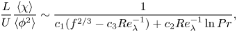 \begin{equation} \frac{L}{U}\frac{\langle\chi\rangle}{\langle\phi^2\rangle} \sim\frac{1}{c_1(f^{2/3}-c_3 Re_\lambda^{{-}1} )+c_2Re_\lambda^{{-}1} \ln Pr},\end{equation}
where  $L$ is the integral length scale of the velocity field, $U$ is the root-mean-square (r.m.s.) velocity, $Re_\lambda$ is the Taylor Reynolds number, $f\equiv A(1+\sqrt {1+(B/Re_\lambda )^2})$ and $A\approx 0.2, B\approx 92, c_1\approx 0.6, c_2\approx (5/3)\sqrt {15}, c_3\approx \sqrt {15}$. These values were determined by fitting the model to DNS data (since the assumed spectra involve unknown $O(1)$ coefficients), except for the factors involving $\sqrt {15}$, which arise due to isotropy of the flow.
The  $\ln Pr$ dependence in (2.10) arises from the contribution due to the Batchelor spectrum for the viscous–convective range. This model predicts that for finite $Pr$,
$Pr$,  $\lim _{Re_\lambda \to \infty }[L\langle \chi \rangle /(U\langle \phi ^2\rangle )]\sim 1/(c_1 2^{2/3} A^{2/3})$, i.e. a constant reflecting anomalous behaviour in this limit. However, for finite $Re_\lambda$ it predicts $\lim _{Pr\to \infty }[L\langle \chi \rangle /(U\langle \phi ^2\rangle )]\sim Re_\lambda /(c_2\ln Pr)$, i.e. no dissipation anomaly. This logarithmic behaviour was confirmed in Donzis et al. (Reference Donzis, Sreenivasan and Yeung2005) at low $Re_\lambda$, and more recently in Buaria et al. (Reference Buaria, Clay, Sreenivasan and Yeung2021b) at a higher Reynolds number $Re_\lambda =140$ over the range $Pr\in [1,512]$. In view of the derivation of (2.10), the interpretation is that the behaviour of $L\langle \chi \rangle /(U\langle \phi ^2\rangle )$ will only be anomalous when the Batchelor regime makes a sub-leading contribution to $L\langle \chi \rangle /(U\langle \phi ^2\rangle )$, and the Obukhov–Corrsin regime dominates.
In addition to the model in (2.10), Donzis et al. (Reference Donzis, Sreenivasan and Yeung2005) also derived a model for  $L\langle \chi \rangle /(U\langle \phi ^2\rangle )$ that applies for $Pr<1$ by integrating the Obukhov–Corrsin spectrum up to the cutoff wavenumber $k\sim 1/\eta _{OC}$. This model also predicts a $Pr$ dependence of $L\langle \chi \rangle /(U\langle \phi ^2\rangle )$, however, in this case it involves $Pr^{1/2}$ rather than the $\ln Pr$ factor that arises for $Pr\geq 1$. The $Pr$ dependence of $L\langle \chi \rangle /(U\langle \phi ^2\rangle )$ only vanishes in the regime $Pr<1$ when $Re_\lambda Pr^{1/2}$ is sufficiently large.
2.2. Behaviour of production terms and the role of ramp-cliff structures
In addition to the de-localization effect that influences the behaviour of  $-\boldsymbol{\mathsf{A}}^\top \boldsymbol {\cdot } \boldsymbol{\mathsf{B}}$ in (2.6) when $Pr>1$, there is a second way in which $Pr$ can influence the stirring processes that govern the amplification of $\boldsymbol{\mathsf{B}}$, which in turn can influence the $Pr$ dependence of $\langle \chi \rangle$. This second effect arises due to a $Pr$-dependent competition between $-\boldsymbol{\mathsf{A}}^\top \boldsymbol {\cdot } \boldsymbol{\mathsf{B}}$ and $N\boldsymbol{\mathsf{A}}^\top \boldsymbol {\cdot } \boldsymbol {e}_z$ in (2.6). This effect was not accounted for in the model of Donzis et al. (Reference Donzis, Sreenivasan and Yeung2005) for $\langle \chi \rangle$ because they assumed that the direct effect of the mean-scalar gradient is unimportant for the behaviour of $\langle \chi \rangle$. Provided that $Re_\lambda \gg 1$ and $Pr\geq O(1)$, we expect $\varLambda _B\ll 1$, reflecting that the fluctuating scalar gradients are much larger than the mean density gradient. As a result, this second effect is usually not important for passive scalars in turbulent flows. Nevertheless, we explain it in significant detail here because it will be shown that it is in fact the main contributor to the strong $Pr$ dependence of $\langle \chi \rangle$ observed for stratified flows in Riley et al. (Reference Riley, Couchman and de Bruyn Kops2023). This therefore provides mechanistic insights into how scalar mixing can differ in significant ways for neutral and stratified flows.
From (2.6) we obtain
 \begin{equation} \tfrac{1}{2}D_t\|\boldsymbol{\mathsf{B}}\|^2=\mathcal{P}_{B1} +\mathcal{P}_{B2} + (\nu/Pr)\nabla^2\|\boldsymbol{\mathsf{B}}\|^2-\mathcal{D}_{B},\end{equation}
where
 \begin{equation} \mathcal{P}_{B1} \equiv{-}\boldsymbol{\mathsf{B}} \boldsymbol{\cdot} \boldsymbol{\mathsf{A}}^\top\boldsymbol{\cdot} \boldsymbol{\mathsf{B}},\end{equation}
is the production term associated with the fluctuating scalar gradient
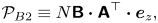 \begin{equation} \mathcal{P}_{B2} \equiv N\boldsymbol{\mathsf{B}} \boldsymbol{\cdot} \boldsymbol{\mathsf{A}}^\top\boldsymbol{\cdot} \boldsymbol{e}_z,\end{equation}
is the production term associated with the mean scalar gradient and  $\mathcal {D}_{B} \equiv (\nu /Pr)\|\boldsymbol {\nabla } \boldsymbol{\mathsf{B}}\|^2$ is the dissipation rate of $\|\boldsymbol{\mathsf{B}}\|^2$.
For a statistically homogeneous flow
 \begin{equation} \tfrac{1}{2}\partial_t\langle\|\boldsymbol{\mathsf{B}}\|^2\rangle=\langle \mathcal{P}_{B1}\rangle+\langle \mathcal{P}_{B2}\rangle-\langle \mathcal{D}_{B}\rangle.\end{equation}
Unlike the dissipation term  $\langle \mathcal {D}_{B}\rangle$, the production terms $\langle \mathcal {P}_{B1}\rangle$ and $\langle \mathcal {P}_{B2}\rangle$ are not sign definite and so may in fact act to oppose the growth of $\langle \|\boldsymbol{\mathsf{B}}\|^2\rangle$ (despite the misnomer, we refer to them as production terms in keeping with the standard terminology used for the production terms in the Reynolds stress equation that are also not sign definite Pope Reference Pope2000). We must therefore consider the sign of these terms in order to understand the role they play in governing $\langle \|\boldsymbol{\mathsf{B}}\|^2\rangle$. It will be shown that the sign of $\langle \mathcal {P}_{B2}\rangle$ is intimately connected to the emergence of ramp-cliff structures in the scalar field, and we therefore first consider in view of (2.6) how these structures form, and then show how this impacts the sign of $\langle \mathcal {P}_{B2}\rangle$ relative to that of $\langle \mathcal {P}_{B1}\rangle$.
When a scalar field is driven by a mean scalar gradient, ramp-cliff structures emerge which are associated with the fluctuating gradients developing a skewness whose sign corresponds to the direction of the imposed mean-scalar gradient (Holzer & Siggia Reference Holzer and Siggia1994; Sreenivasan Reference Sreenivasan2018; Buaria et al. Reference Buaria, Clay, Sreenivasan and Yeung2021a). To understand how this asymmetry arises from the equation for  $\boldsymbol{\mathsf{B}}$, we may consider the case where the probability density function (p.d.f.) of the initial condition $\boldsymbol{\mathsf{B}}(0)$ is an isotropic and symmetric function, and uncorrelated from $\boldsymbol{\mathsf{A}}$. Writing $\boldsymbol{\mathsf{B}}$ in terms of Cartesian components, the equation for $B_z\equiv \boldsymbol{\mathsf{B}} \boldsymbol {\cdot } \boldsymbol {e}_z$ is obtained from (2.6)
 \begin{equation} D_t{B}_z={-}B_x A_{xz}-B_y A_{yz}-(B_z-N) A_{zz}+(\nu/Pr)\nabla^2B_z, \end{equation}
where subscripts  $x$ and $y$ denote components in the horizontal directions of the flow. For an isotropic flow, the p.d.f.s of $A_{xz}$ and $A_{yz}$ are symmetric. Therefore, given the symmetric initial condition for $\boldsymbol{\mathsf{B}}$, the symmetry breaking responsible for the p.d.f. of $B_z$ becoming skewed cannot come from the terms $-B_x A_{xz}-B_y A_{yz}$ (or $\nabla ^2B_z$), but must come from $-(B_z-N) A_{zz}$. The strongest symmetry breaking associated with this term is generated in the range $|B_z|\in [0,N)$ and so we focus on this range. In the range $|B_z|\in [0,N)$ we can write $-(B_z-N) A_{zz}=|B_z-N| A_{zz}$, and so $A_{zz}<0$ events drive $B_z$ towards negative values, while $A_{zz}>0$ events drive $B_z$ towards positive values. Since in an isotropic flow, the p.d.f. of $A_{zz}$ is negatively skewed, then the term $|B_z-N| A_{zz}$ will generate larger negative values of $B_z$ than positive ones, and hence negative skewness. If the flow field were Gaussian, however, this mechanism would be absent. Nevertheless, random Gaussian flows also generate skewed p.d.f.s for $B_z$ (Holzer & Siggia Reference Holzer and Siggia1994) and, therefore, there must be another mechanism responsible for this. This second mechanism arises from the fact that, starting from the isotropic initial condition for $B_z(0)$ and in a flow where the p.d.f. of $A_{zz}$ is symmetric, statistically $-(B_z(0)-N) A_{zz}$ will be larger in regions where $B_z(0)<0$ than in regions where $B_z(0)>0$. This means that $-(B_z(0)-N) A_{zz}$ will generate larger negative values of $B_z$ than positive ones, and hence negative skewness. This mechanism fundamentally arises in (2.6) due to the ability of the fluctuating production $-\boldsymbol{\mathsf{A}}^\top \boldsymbol {\cdot } \boldsymbol{\mathsf{B}}$ and mean gradient production $N\boldsymbol{\mathsf{A}}^\top \boldsymbol {\cdot } \boldsymbol {e}_z$ terms to act together or against each other, and skewness of the p.d.f. will be generated in the direction for which the two terms act together. The same argument applied to the case $\gamma >0$ shows that in this case, $B_z$ will be positively skewed, the opposite of the $\gamma <0$ case.
In view of this, the emergence of ramp-cliff structures is determined by the interplay between  $-\boldsymbol{\mathsf{A}}^\top \boldsymbol {\cdot } \boldsymbol{\mathsf{B}}$ and $N\boldsymbol{\mathsf{A}}^\top \boldsymbol {\cdot } \boldsymbol {e}_z$, which are associated with the production terms $\mathcal {P}_{B1}$ and $\mathcal {P}_{B2}$ in (2.11). It may therefore be anticipated that ramp-cliff structures are also relevant to understanding the signs of the average terms $\langle \mathcal {P}_{B1}\rangle$ and $\langle \mathcal {P}_{B2}\rangle$. To consider this, we begin by examining the behaviour of $\langle \mathcal {P}_{B1}\rangle$ and $\langle \mathcal {P}_{B2}\rangle$ in the ‘short-time regime’ for the case where scalars are introduced to a fully developed turbulent flow with initial condition $\boldsymbol{\mathsf{B}}(\boldsymbol {x},0)=\boldsymbol {0}\,\forall \boldsymbol {x}$ (a situation that will be of relevance to the DNS shown later). Using the Kolmogorov time scale $\tau _\eta$, for $t\ll \tau _\eta$ we have $\tau _\eta \boldsymbol{\mathsf{A}}(t)=\tau _\eta \boldsymbol{\mathsf{A}}(0) +O(t/\tau _\eta )$, and inserting this into (2.6) yields the solution $\tau _\eta \boldsymbol{\mathsf{B}}(t)\sim \tau _\eta N t\boldsymbol{\mathsf{A}}^\top (0)\boldsymbol {\cdot } \boldsymbol {e}_z+O([t/\tau _\eta ]^2)$ when $\boldsymbol{\mathsf{B}}(0)=\boldsymbol {0}$. From this we obtain for $t\ll \tau _\eta$
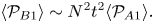
 \begin{equation} \langle \mathcal{P}_{B2}\rangle\sim N^2 t\langle\|\boldsymbol{\mathsf{A}}^\top(0)\boldsymbol{\cdot} \boldsymbol{e}_z\|^2\rangle, \end{equation}
and hence at short times  $\langle \mathcal {P}_{B2}\rangle >0$. Using the same approach we can also derive
 \begin{equation} \langle \mathcal{P}_{B1}\rangle \sim N^2 t^2\langle\mathcal{P}_{A1}\rangle. \end{equation}
The invariant
 \begin{equation} \mathcal{P}_{A1}\equiv{-}\boldsymbol{\mathsf{A}}^\top\boldsymbol{:}(\boldsymbol{\mathsf{A}}\boldsymbol{\cdot} \boldsymbol{\mathsf{A}}),\end{equation}
is the velocity gradient self-amplification term and it is positive on average (Tsinober Reference Tsinober2000) so that it acts as a source term in the equation for  $\partial _t\langle \|\boldsymbol{\mathsf{A}}\|^2\rangle$. As a result $\langle \mathcal {P}_{B1}\rangle >0$ at short times, but its contribution is sub-leading compared with that from the mean gradient production term $\langle \mathcal {P}_{B2}\rangle$.
The question is whether the sign of these production terms remains the same once the stationary regime  $\partial _t\langle \|\boldsymbol{\mathsf{B}}\|^2\rangle = 0$ has been attained where the ramp-cliff structures are fully developed. The production terms may be re-expressed using $\boldsymbol{\mathsf{B}}=\|\boldsymbol{\mathsf{B}}\|\boldsymbol {e}_B$ and index notation as
 $$\begin{gather} \langle \mathcal{P}_{B1}\rangle ={-}\langle\|\boldsymbol{\mathsf{B}}\|^2 (\boldsymbol{e}_{\boldsymbol B}\boldsymbol{\cdot} \boldsymbol{e}_j) A_{ji}(\boldsymbol{e}_i\boldsymbol{\cdot} \boldsymbol{e}_{\boldsymbol B})\rangle, \end{gather}$$
 $$\begin{gather}\langle \mathcal{P}_{B2}\rangle =N\langle\|\boldsymbol{\mathsf{B}}\| (\boldsymbol{e}_{\boldsymbol B}\boldsymbol{\cdot} \boldsymbol{e}_j) A_{ji}(\boldsymbol{e}_i\boldsymbol{\cdot} \boldsymbol{e}_z)\rangle, \end{gather}$$
where  $\boldsymbol {e}_i$ are the basis vectors for the Cartesian coordinate system, with $i,j\in \{x,y,z\}$. Written in this form it is clear that these terms will only have the same sign if $\boldsymbol {e}_i\boldsymbol {\cdot } \boldsymbol {e}_{\boldsymbol B}$ and $\boldsymbol {e}_i\boldsymbol {\cdot } \boldsymbol {e}_z$ tend to have opposite signs (since we are considering $N> 0$). This, in turn, depends on the alignments of $\boldsymbol {e}_{\boldsymbol B}$ and $\boldsymbol {e}_z$, which are connected to the formation of the ramp-cliff structures in the flow.
Since  $\langle \phi \rangle =0$ then $\langle B_z\rangle =0$, because $\langle B_z\rangle =\langle \nabla _z \phi \rangle =\nabla _z\langle \phi \rangle =0$. Ramp-cliff structures are associated with $B_z$ having larger negative than positive values (when $\gamma <0$), such that the odd moments of $B_z$ are negative. However, in order for $\langle B_z\rangle =0$ to be satisfied, it must be the case that events where $B_z>0$ are more probable than those with $B_z<0$. Since $B_z=\|\boldsymbol{\mathsf{B}}\|\boldsymbol {e}_{\boldsymbol B}\boldsymbol {\cdot } \boldsymbol {e}_z$, a higher probability of $B_z>0$ events corresponds to a higher probability of $\boldsymbol {e}_{\boldsymbol B}\boldsymbol {\cdot } \boldsymbol {e}_z>0$ events than $\boldsymbol {e}_{\boldsymbol B}\boldsymbol {\cdot } \boldsymbol {e}_z<0$ events. Due to this, the most probable configuration is that the signs of $\boldsymbol {e}_i\boldsymbol {\cdot } \boldsymbol {e}_z$ and $\boldsymbol {e}_i\boldsymbol {\cdot } \boldsymbol {e}_{\boldsymbol B}$ will be the same, and therefore once ramp-cliff structures emerge in the field, the production terms $\langle \mathcal {P}_{B1}\rangle$ and $\langle \mathcal {P}_{B2}\rangle$ will have opposite signs.
This argument establishes that  $\langle \mathcal {P}_{B1}\rangle$ and $\langle \mathcal {P}_{B2}\rangle$ will have opposite signs once ramp-cliff structures in the flow have developed. The argument does not depend on how strong the ramp-cliff structures are, but only that they exist, such that the probability distribution of $\boldsymbol {e}_{\boldsymbol B} \boldsymbol {\cdot }\boldsymbol {e}_z$ is not strictly uniform. Therefore, although the ramp-cliff structures for a passive scalar are known to weaken as $Pr$ is increased beyond $Pr=1$, with the skewness of $B_z$ asymptotically approaching zero in the limit $Pr\to \infty$ (Buaria et al. Reference Buaria, Clay, Sreenivasan and Yeung2021a; Shete et al. Reference Shete, Boucher, Riley and de Bruyn Kops2022), $\langle \mathcal {P}_{B1}\rangle$ and $\langle \mathcal {P}_{B2}\rangle$ will have opposite signs at all finite $Pr$. The argument given above does not, however, establish the sign of $\langle \mathcal {P}_{B2}\rangle$, but only that its sign must be opposite to that of $\langle \mathcal {P}_{B1}\rangle$. To determine the sign of $\langle \mathcal {P}_{B2}\rangle$ we would also have to consider the behaviour of $\|\boldsymbol{\mathsf{B}}\|$ and $A_{ji}$ in the expression $\langle \mathcal {P}_{B2}\rangle =N\langle \|{\boldsymbol{B}}\| (\boldsymbol {e}_{\boldsymbol{B}}\boldsymbol {\cdot } \boldsymbol{e}_j) A_{ji}(\boldsymbol {e}_i\boldsymbol {\cdot } \boldsymbol {e}_z)\rangle$. We can, however, infer its sign by the following argument: in order for the stationary regime $\partial _t\langle \|\boldsymbol{\mathsf{B}}\|^2\rangle = 0$ to be sustained, it must be that case that $\langle \mathcal {P}_{B1}\rangle +\langle \mathcal {P}_{B2}\rangle >0$. If $\varLambda _B<1$, then according to the scaling introduced in § 2, $|\langle \mathcal {P}_{B1}\rangle |>|\langle \mathcal {P}_{B2}\rangle |$, and it therefore follows from the argument above that we must have $\langle \mathcal {P}_{B1}\rangle >0$ and $\langle \mathcal {P}_{B2}\rangle <0$ in the stationary regime due to the ramp-cliff structures.
2.3. The importance of the mean-scalar gradient production
Since  $\langle \mathcal {P}_{B2}\rangle <0$, then the mean-scalar gradient term $\langle \mathcal {P}_{B2}\rangle$ acts to oppose the growth of $\langle \|\boldsymbol{\mathsf{B}}\|^2\rangle$, and hence acts to decrease the scalar dissipation rate $\langle \chi \rangle$. In the passive scalar limit, high Reynolds number turbulent flows with $Pr\geq O(1)$ will exist in the regime $\varLambda _B\ll 1$ due to the fluctuating scalar gradients being much larger than the mean scalar gradient. Therefore, the effect of $\langle \mathcal {P}_{B2}\rangle$ on $\langle \chi \rangle$ is expected to be negligible in the high Reynolds number passive scalar regime where $|\langle \mathcal {P}_{B2}\rangle |/|\langle \mathcal {P}_{B1}\rangle |\sim O(\varLambda _B)\ll 1$, which we will later confirm with DNS data.
The mean-scalar gradient term must nevertheless play a crucial implicit role because without it the fluctuating scalar gradients would decay. To see this more clearly we should consider the behaviour of the filtered gradients which provide information about the scalar gradients at different scales.
We define the filtering operation for an arbitrary field quantity  $\boldsymbol {Y}$ to be
 \begin{equation} \tilde{\boldsymbol{Y}}(\boldsymbol{x},t)\equiv \int_{\mathbb{R}^3}\mathcal{G}_\ell(\|\boldsymbol{x}- \boldsymbol{x}'\|)\boldsymbol{Y}(\boldsymbol{x}',t)\,{\rm d}\kern0.7pt\boldsymbol{x}', \end{equation}
where  $\mathcal {G}_\ell$ is an isotropic filter kernel with filtering length scale $\ell$ (the particular choice of kernel, e.g. a Gaussian or box function, is not important here). Applying this filtering operator to (2.2) and taking the gradient of the resulting equation leads to
 \begin{equation} \tilde{D}_t\tilde{\boldsymbol{\mathsf{B}}}={-}\tilde{\boldsymbol{\mathsf{A}}}^\top \boldsymbol{\cdot} \tilde{\boldsymbol{\mathsf{B}}}+(\nu/Pr)\nabla^2 \tilde{\boldsymbol{\mathsf{B}}}+N\tilde{\boldsymbol{\mathsf{A}}}^\top \boldsymbol{\cdot} \boldsymbol{e}_z-\boldsymbol{\nabla}\boldsymbol{\nabla}\boldsymbol{\cdot} \boldsymbol{\tau}_\phi,\end{equation}
where  $\tilde {D}_t\equiv \partial _t+(\tilde {\boldsymbol {u}}\boldsymbol {\cdot }\boldsymbol {\nabla } )$, and $\boldsymbol {\tau }_\phi \equiv \widetilde{\boldsymbol {u}\phi }- \tilde {\boldsymbol {u}}\tilde {\phi }$ is the sub-grid stress vector.
From (2.22), the equation governing  $\partial _t\langle \|\tilde {\boldsymbol{\mathsf{B}}}\|^2\rangle$ can be constructed, and for a statistically stationary, homogeneous flow it reduces to
 \begin{equation} 0={-}\langle \tilde{\boldsymbol{\mathsf{B}}}\boldsymbol{\cdot} \tilde{\boldsymbol{\mathsf{A}}}^\top\boldsymbol{\cdot} \tilde{\boldsymbol{\mathsf{B}}}\rangle-(\nu/Pr)\langle\|\boldsymbol{\nabla} \tilde{\boldsymbol{\mathsf{B}}}\|^2\rangle+N\langle \tilde{\boldsymbol{\mathsf{B}}}\boldsymbol{\cdot} \tilde{\boldsymbol{\mathsf{A}}}^\top \boldsymbol{\cdot} \boldsymbol{e}_z\rangle-\langle \tilde{\boldsymbol{\mathsf{B}}}\boldsymbol{\cdot} \boldsymbol{\nabla}\boldsymbol{\nabla}\boldsymbol{\cdot} \boldsymbol{\tau}_\phi\rangle. \end{equation}
For  $\ell \gg \eta _B$, where $\eta _B$ is the Batchelor length scale, the dissipation term $(\nu /Pr)\langle \|\boldsymbol {\nabla } \tilde {\boldsymbol{\mathsf{B}}}\|^2\rangle$ can be ignored because almost all of the scalar dissipation takes place at scales $\ell =O(\eta _B)$. Therefore, for $\ell \gg \eta _B$ we have the balance
 \begin{equation} {-}\langle \tilde{\boldsymbol{\mathsf{B}}}\boldsymbol{\cdot} \tilde{\boldsymbol{\mathsf{A}}}^\top \boldsymbol{\cdot} \tilde{\boldsymbol{\mathsf{B}}}\rangle+N\langle \tilde{\boldsymbol{\mathsf{B}}}\boldsymbol{\cdot} \tilde{\boldsymbol{\mathsf{A}}}^\top \boldsymbol{\cdot} \boldsymbol{e}_z\rangle\sim \langle \tilde{\boldsymbol{\mathsf{B}}}\boldsymbol{\cdot} \boldsymbol{\nabla}\boldsymbol{\nabla}\boldsymbol{\cdot} \boldsymbol{\tau}_\phi\rangle.\end{equation}
The term  $\langle \tilde {\boldsymbol{\mathsf{B}}}\boldsymbol {\cdot } \boldsymbol {\nabla }\boldsymbol {\nabla }\boldsymbol {\cdot } \boldsymbol {\tau }_\phi \rangle$ will be positive because this term describes how fluctuations are transferred on average to the sub-grid gradients from the filtered gradients, analogous to the kinetic and scalar variance cascades which are downscale in three dimensions.
Using the same scaling approach discussed in § 2 but now for the filtered variables leads to
 \begin{equation} \frac{|N\langle \tilde{\boldsymbol{\mathsf{B}}}\boldsymbol{\cdot} \tilde{\boldsymbol{\mathsf{A}}}^\top \boldsymbol{\cdot} \boldsymbol{e}_z\rangle|}{|\langle \tilde{\boldsymbol{\mathsf{B}}}\boldsymbol{\cdot} \tilde{\boldsymbol{\mathsf{A}}}^\top \boldsymbol{\cdot} \tilde{\boldsymbol{\mathsf{B}}}\rangle|}\sim O(\tilde{\varLambda}_B), \end{equation}
where  $\tilde {\varLambda }_B\equiv N/\sqrt {\langle \|\tilde {\boldsymbol{\mathsf{B}}}\|^2\rangle }$. Therefore, at scales where $\tilde {\varLambda }_B\ll 1$, the balance reduces to
 \begin{equation} {-}\langle \tilde{\boldsymbol{\mathsf{B}}}\boldsymbol{\cdot} \tilde{\boldsymbol{\mathsf{A}}}^\top \boldsymbol{\cdot} \tilde{\boldsymbol{\mathsf{B}}}\rangle\sim \langle \tilde{\boldsymbol{\mathsf{B}}}\boldsymbol{\cdot} \boldsymbol{\nabla}\boldsymbol{\nabla}\boldsymbol{\cdot} \boldsymbol{\tau}_\phi\rangle, \end{equation}
while at scales where  $\tilde {\varLambda }_B\gg 1$ the balance reduces to
 \begin{equation} N\langle \tilde{\boldsymbol{\mathsf{B}}}\boldsymbol{\cdot} \tilde{\boldsymbol{\mathsf{A}}}^\top \boldsymbol{\cdot} \boldsymbol{e}_z\rangle\sim \langle \tilde{\boldsymbol{\mathsf{B}}}\boldsymbol{\cdot} \boldsymbol{\nabla}\boldsymbol{\nabla}\boldsymbol{\cdot} \boldsymbol{\tau}_\phi\rangle. \end{equation}
Since  $\langle \tilde {\boldsymbol{\mathsf{B}}}\boldsymbol {\cdot } \boldsymbol {\nabla }\boldsymbol {\nabla }\boldsymbol {\cdot } \boldsymbol {\tau }_\phi \rangle >0$, then we must have $N\langle \tilde {\boldsymbol{\mathsf{B}}}\boldsymbol {\cdot } \tilde {\boldsymbol{\mathsf{A}}}^\top \boldsymbol {\cdot } \boldsymbol {e}_z\rangle >0$ at scales where $\tilde {\varLambda }_B\gg 1$ in order for the balance to be satisfied. Therefore, although $\lim _{\ell /\eta _B\to 0}N\langle \tilde {\boldsymbol{\mathsf{B}}}\boldsymbol {\cdot } \tilde {\boldsymbol{\mathsf{A}}}^\top \boldsymbol {\cdot } \boldsymbol {e}_z\rangle \to \langle \mathcal {P}_{B2}\rangle$ is predicted to be negative due to the ramp-cliff structures, at scales where $\tilde {\varLambda }_B\gg 1$ is satisfied then $N\langle \tilde {\boldsymbol{\mathsf{B}}}\boldsymbol {\cdot } \tilde {\boldsymbol{\mathsf{A}}}^\top \boldsymbol {\cdot } \boldsymbol {e}_z\rangle >0$. Hence, the role of this mean gradient term in the equation governing $\langle \|\tilde {\boldsymbol{\mathsf{B}}}\|^2\rangle$ changes with scale, providing a source for $\langle \|\tilde {\boldsymbol{\mathsf{B}}}\|^2\rangle$ at scales where $\tilde {\varLambda }_B\gg 1$, and providing a sink for $\langle \|\tilde {\boldsymbol{\mathsf{B}}}\|^2\rangle$ at scales where $\tilde {\varLambda }_B\ll 1$.
Note that regardless of  $Re_\lambda$ or $Pr$, there will always be a range of scales where $\tilde {\varLambda }_B\gg 1$ is satisfied because statistical homogeneity of the flow enforces that $\lim _{\ell /L_\phi \to \infty }\tilde {\boldsymbol{\mathsf{B}}}\to 0$ (where $L_\phi$ is the integral length scale of $\phi$), i.e. for sufficiently large scales, $\tilde {\boldsymbol{\mathsf{B}}}$ is equivalent to the spatial average of $\boldsymbol{\mathsf{B}}$, which is zero. Due to this, $\lim _{\ell /L_\phi \to \infty }\tilde {\varLambda }_B\to \infty$, regardless of $Re_\lambda$ or $Pr$.
$Pr$.
3. Theory: gradient dynamics in stably stratified turbulence
Having considered the case of passive scalars we now turn to consider stably stratified turbulence. We will see that some of the effects that are already present for passive scalars play an important role in understanding stratified turbulence, and in particular, the role of  $\langle \mathcal {P}_{B2}\rangle$. As discussed earlier, the term $\langle \mathcal {P}_{B2}\rangle$ is expected to be unimportant compared with $\langle \mathcal {P}_{B1}\rangle$ for passive scalars in turbulent flows for which the particular value of $N$ (on which $\langle \mathcal {P}_{B2}\rangle$ explicitly depends) is essentially irrelevant due to the linearity of the scalar equation. This is not true for stratified turbulent flows, however, because the momentum equation depends on $N$ through the buoyancy term, and the momentum equation is nonlinear. Therefore, we anticipate that $\langle \mathcal {P}_{B2}\rangle$ could play an important role in stratified turbulence, and this suggests that the striking effect of $Pr$ on $\langle \epsilon \rangle$ and $\langle \chi \rangle$ observed in Riley et al. (Reference Riley, Couchman and de Bruyn Kops2023), which is much stronger than the $Pr$ effect on $\langle \chi \rangle$ for passive scalars, could be connected to a $Pr$-dependence of $\langle \mathcal {P}_{B2}\rangle$.
3.1. Buoyancy acts as both a source and a sink for velocity gradients in stratified turbulence
The only difference between the gradient dynamics of passive scalar turbulence and stratified turbulence is the buoyancy term in the equation for  $\boldsymbol{\mathsf{S}}$. For a statistically homogeneous flow, the equation governing $\langle \|\boldsymbol{\mathsf{S}}\|^2\rangle$ reduces to
 \begin{equation} \frac{1}{2}\partial_t\langle\|\boldsymbol{\mathsf{S}}\|^2\rangle =\langle\mathcal{P}_{S1}\rangle-\frac{N}{2}\langle \boldsymbol{\mathsf{S}}\boldsymbol{:}(\boldsymbol{\mathsf{B}}\boldsymbol{e}_z+ \boldsymbol{e}_z\boldsymbol{\mathsf{B}})\rangle-\langle \mathcal{D}_{S}\rangle+\langle\mathcal{P}_{S2}\rangle,\end{equation}
from which the pressure gradient term has disappeared because  $\langle \boldsymbol{\mathsf{S}}\boldsymbol {:}\boldsymbol {\nabla }\boldsymbol {\nabla } p\rangle =0$ for an incompressible, homogeneous flow. In this equation
 \begin{equation} \mathcal{P}_{S1}\equiv{-}\boldsymbol{\mathsf{S}}\boldsymbol{:}\boldsymbol{\mathsf{S}}\boldsymbol{\cdot} \boldsymbol{\mathsf{S}}-(1/4) \boldsymbol{\mathsf{S}}\boldsymbol{:}\boldsymbol{\omega\omega},\end{equation}
where  $-\boldsymbol{\mathsf{S}}\boldsymbol {:}\boldsymbol{\mathsf{S}}\boldsymbol {\cdot } \boldsymbol{\mathsf{S}}$ is the strain self-amplification invariant, and $\boldsymbol{\mathsf{S}}\boldsymbol {:}\boldsymbol {\omega \omega }$ is the enstrophy production invariant associated with the process of vortex stretching (Tsinober Reference Tsinober2001). In a turbulent flow, $\langle \mathcal {P}_{S1}\rangle >0$, reflecting the fact that nonlinearity in the flow self-amplifies the straining motion. We also note that using the results from Betchov (Reference Betchov1956) for an incompressible, homogeneous flow, it can be shown that $\langle \mathcal {P}_{S1}\rangle =(1/2)\langle \mathcal {P}_{A1}\rangle$, where $\mathcal {P}_{A1}$ is defined in (2.18). The dissipation term is $\mathcal {D}_{S}\equiv \nu \|\boldsymbol {\nabla } \boldsymbol{\mathsf{S}}\|^2$, and $\mathcal {P}_{S2}\equiv \,\boldsymbol{\mathsf{S}}\boldsymbol {:}\boldsymbol {\nabla } \boldsymbol {F}_S$, which describes the contribution to the strain from the forcing (which is usually negligible in the equation for a high Reynolds number flow).
The buoyancy term that appears in (3.1) is  $-(N/2)\langle \boldsymbol{\mathsf{S}}\boldsymbol {:}(\boldsymbol{\mathsf{B}}\boldsymbol {e}_z+ \boldsymbol {e}_z\boldsymbol{\mathsf{B}})\rangle$. However, it is straightforward to show that for an incompressible, homogeneous flow $\langle \boldsymbol{\mathsf{S}}\boldsymbol {:}(\boldsymbol{\mathsf{B}}\boldsymbol {e}_z+ \boldsymbol {e}_z\boldsymbol{\mathsf{B}})\rangle =\langle \boldsymbol{\mathsf{B}} \boldsymbol {\cdot } \boldsymbol{\mathsf{A}}^\top \boldsymbol {\cdot } \boldsymbol {e}_z \rangle$, and therefore the buoyancy term in (3.1) is equal to $-(1/2)\langle \mathcal {P}_{B2}\rangle$. It was argued in § 2.2 that for a passive scalar with $\boldsymbol{\mathsf{B}}(0)=\boldsymbol {0}$, for $t\ll \tau _\eta$ we have $\langle \mathcal {P}_{B2}\rangle >0$, however, once the ramp-cliff structures form and the stationary regime $\partial _t\langle \|\boldsymbol{\mathsf{B}}\|^2\rangle = 0$ is attained, $\langle \mathcal {P}_{B2}\rangle <0$. The argument that $\langle \mathcal {P}_{B2}\rangle <0$ at long times is statistical in nature, and depends only on the assumption that there are ramp-cliff structures in the flow which correspond to a higher probability of $\boldsymbol {e}_{\boldsymbol B}\boldsymbol {\cdot } \boldsymbol {e}_z>0$ events than $\boldsymbol {e}_{\boldsymbol B}\boldsymbol {\cdot } \boldsymbol {e}_z<0$ events. Since ramp-cliff structures also occur in stratified flows (Riley et al. Reference Riley, Couchman and de Bruyn Kops2023) then the arguments given in § 2.2 regarding the sign of $\langle \mathcal {P}_{B2}\rangle$ also apply to stratified flows. Therefore, since $-(N/2)\langle \boldsymbol{\mathsf{S}}\boldsymbol {:}(\boldsymbol{\mathsf{B}}\boldsymbol {e}_z+ \boldsymbol {e}_z\boldsymbol{\mathsf{B}})\rangle =-(1/2)\langle \mathcal {P}_{B2}\rangle$, then the buoyancy term in (3.1) will act as a sink term for $t\ll \tau _\eta$, but will act as a source term once $\langle \mathcal {P}_{B2}\rangle <0$ is established, contributing to the growth of $\langle \|\boldsymbol{\mathsf{S}}\|^2\rangle$, and hence acting to increase $\langle \epsilon \rangle =2\nu \langle \|\boldsymbol{\mathsf{S}}\|^2\rangle$. Moreover, since $2\langle \|\boldsymbol{\mathsf{S}}\|^2\rangle =\langle \|\boldsymbol {\omega }\|^2\rangle$ for an incompressible, homogeneous flow (Betchov Reference Betchov1956), this also implies that buoyancy acts to increase enstrophy in the flow.
This conclusion seems surprising, because in stably stratified turbulence, buoyancy is expected to play the role of a sink term for turbulence. To understand the role of buoyancy on the velocity gradients in more detail we can use the filtering approach introduced earlier. Applying the filtering operator to (2.1) and taking the gradient of the resulting equation yields
 \begin{equation} \tilde{D}_t\tilde{\boldsymbol{\mathsf{A}}}={-}\tilde{\boldsymbol{\mathsf{A}}} \boldsymbol{\cdot} \tilde{\boldsymbol{\mathsf{A}}}-\boldsymbol{\nabla}\boldsymbol{\nabla} \tilde{p}+\nu\nabla^2\tilde{\boldsymbol{\mathsf{A}}}-N\tilde{\boldsymbol{\mathsf{B}}} \boldsymbol{e}_z+\boldsymbol{\nabla} \tilde{\boldsymbol{F}}- \boldsymbol{\nabla}\boldsymbol{\nabla}\boldsymbol{\cdot} \boldsymbol{\tau}_{\boldsymbol u},\end{equation}
where  $\boldsymbol {\tau }_{\boldsymbol u}\equiv \widetilde {\boldsymbol {uu}}- \tilde {\boldsymbol {u}}\tilde {\boldsymbol {u}}$ is the sub-grid stress tensor. From (3.3), the equation governing $\partial _t\langle \|\tilde {\boldsymbol{\mathsf{A}}}\|^2\rangle$ can be constructed, and for a statistically stationary, homogeneous flow it reduces to
 \begin{equation} 0={-}\langle\tilde{\boldsymbol{\mathsf{A}}}\boldsymbol{:}(\tilde{\boldsymbol{\mathsf{A}}} \boldsymbol{\cdot} \tilde{\boldsymbol{\mathsf{A}}})\rangle- \nu\langle\|\boldsymbol{\nabla} \tilde{\boldsymbol{\mathsf{A}}}\|^2\rangle-N\langle \tilde{\boldsymbol{\mathsf{B}}}\boldsymbol{\cdot} \tilde{\boldsymbol{\mathsf{A}}}^\top \boldsymbol{\boldsymbol{\cdot} e}_z\rangle+\langle\tilde{\boldsymbol{\mathsf{A}}}\boldsymbol{:} \boldsymbol{\nabla} \tilde{\boldsymbol{F}}\rangle-\langle \tilde{\boldsymbol{\mathsf{A}}}\boldsymbol{:}\boldsymbol{\nabla}\boldsymbol{\nabla}\boldsymbol{\cdot} \boldsymbol{\tau}_{\boldsymbol u}\rangle. \end{equation}
Once again, the pressure gradient term does not appear because  $\langle \tilde {\boldsymbol{\mathsf{A}}}\boldsymbol {:}\boldsymbol {\nabla }\boldsymbol {\nabla }\tilde {p}\rangle =0$ for an incompressible, homogeneous flow. The term $\langle \tilde {\boldsymbol{\mathsf{A}}}\boldsymbol {:}\boldsymbol {\nabla }\boldsymbol {\nabla }\boldsymbol {\cdot } \boldsymbol {\tau }_{\boldsymbol u}\rangle$ will be positive because this term describes how fluctuations are transferred on average to the sub-grid gradients from the filtered gradients, analogous to the kinetic energy cascade which is downscale in three dimensional stratified turbulence (Lindborg Reference Lindborg2006).
For  $\ell \gg \eta$ the dissipation term $\nu \langle \|\boldsymbol {\nabla } \tilde {\boldsymbol{\mathsf{A}}}\|^2\rangle$ can be ignored because almost all of the dissipation takes place at scales $\ell =O(\eta )$, leading to the reduced balance
 \begin{equation} \langle\tilde{\boldsymbol{\mathsf{A}}}\boldsymbol{:}\boldsymbol{\nabla} \tilde{\boldsymbol{F}}\rangle\sim\langle\tilde{\boldsymbol{\mathsf{A}}}\boldsymbol{:}(\tilde{\boldsymbol{\mathsf{A}}}\boldsymbol{\cdot} \tilde{\boldsymbol{\mathsf{A}}})\rangle+N\langle \tilde{\boldsymbol{\mathsf{B}}}\boldsymbol{\cdot} \tilde{\boldsymbol{\mathsf{A}}}^\top \boldsymbol{\cdot} \boldsymbol{e}_z\rangle+\langle\tilde{\boldsymbol{\mathsf{A}}}\boldsymbol{:}\boldsymbol{\nabla}\boldsymbol{\nabla}\boldsymbol{\cdot} \boldsymbol{\tau}_{\boldsymbol u}\rangle.\end{equation}
Using the same scaling approach discussed in § 2 but now for the filtered variables leads to
 $$\begin{gather} \frac{|N\langle \tilde{\boldsymbol{\mathsf{B}}}\boldsymbol{\cdot} \tilde{\boldsymbol{\mathsf{A}}}^\top \boldsymbol{\cdot} \boldsymbol{e}_z\rangle|}{|\langle\tilde{\boldsymbol{\mathsf{A}}}\boldsymbol{:} (\tilde{\boldsymbol{\mathsf{A}}}\boldsymbol{\cdot} \tilde{\boldsymbol{\mathsf{A}}})\rangle|}\sim O(\tilde{\varLambda}_A), \end{gather}$$
 $$\begin{gather}\tilde{\varLambda}_A \equiv \frac{N\langle\|\tilde{\boldsymbol{\mathsf{B}}}\|^2\rangle^{1/2}}{\langle\| \tilde{\boldsymbol{\mathsf{A}}}\|^2\rangle}. \end{gather}$$
In the regime  $\tilde {\varLambda }_A\gg 1$ the balance in (3.5) reduces to
 \begin{equation} \langle\tilde{\boldsymbol{\mathsf{A}}}\boldsymbol{:}\boldsymbol{\nabla} \tilde{\boldsymbol{F}}\rangle\sim N\langle \tilde{\boldsymbol{\mathsf{B}}}\boldsymbol{\cdot} \tilde{\boldsymbol{\mathsf{A}}}^\top \boldsymbol{\cdot} \boldsymbol{e}_z\rangle+\langle\tilde{\boldsymbol{\mathsf{A}}}\boldsymbol{:}\boldsymbol{\nabla}\boldsymbol{\nabla}\boldsymbol{\cdot} \boldsymbol{\tau}_{\boldsymbol u}\rangle,\end{equation}
and if we also have  $\tilde {\varLambda }_B\gg 1$ then as shown in § 2.3, $N\langle \tilde {\boldsymbol{\mathsf{B}}}\boldsymbol {\cdot } \tilde {\boldsymbol{\mathsf{A}}}^\top \boldsymbol {\cdot } \boldsymbol {e}_z\rangle >0$. This represents the balance at relatively large scales where the production term due to forcing is balanced by losses due to buoyancy and transfer to smaller scales (which is analogous to the TKE equation (2.3) because the TKE is dominated by the large scales in high Reynolds number flows). The role of the buoyancy term $-N\langle \tilde {\boldsymbol{\mathsf{B}}}\boldsymbol {\cdot } \tilde {\boldsymbol{\mathsf{A}}}^\top \boldsymbol {\cdot } \boldsymbol {e}_z\rangle$ is therefore subtle, opposing the production of velocity gradients at scales where $\tilde {\varLambda }_B\gg 1$, but aiding their production at scales where $\tilde {\varLambda }_B\ll 1$. This must be connected to the observation in Legaspi & Waite (Reference Legaspi and Waite2020) based on their numerical simulations that the buoyancy spectrum changes sign and indicates transfer of potential energy to kinetic energy at high wavenumbers in stratified turbulence. An investigation into this connection will be the subject of future work.
Note that in a flow where  $\tilde {\varLambda }_B\geq O(1)\ \forall \, \ell$, the buoyancy term will act as a sink term for the velocity gradients at all scales and corresponds to the case where buoyancy is strong enough to suppress turbulence at all scales.
3.2. Prandtl number dependence of the kinetic and potential energy dissipation rates
Having considered how stratification impacts the velocity gradients through the buoyancy term, we now want to understand the impact of varying  $Pr$ in order to understand how $Pr$ affects $\langle \epsilon \rangle$ and $\langle \chi \rangle$ in stratified turbulence. Although a general analytical treatment of this problem is not possible, we can obtain some insights by considering a limiting case.
In § 2 the following scaling estimate was obtained:
 \begin{equation} \frac{\|-(N/2)(\boldsymbol{\mathsf{B}}\boldsymbol{e}_z+\boldsymbol{e}_z \boldsymbol{\mathsf{B}})\|}{\|-\boldsymbol{\mathsf{S}}\boldsymbol{\cdot} \boldsymbol{\mathsf{S}}-(1/4)(\boldsymbol{\omega\omega}-\|\boldsymbol{\omega}\|^2 \boldsymbol{I})-\boldsymbol{\nabla}\boldsymbol{\nabla} p\|}\sim O(\varLambda_S), \end{equation}
and given that the equation is regular in the limit  $\varLambda _S\to 0$, this suggests that we can use $\varLambda _S$ as an expansion parameter and consider the regime $\varLambda _S \ll 1$ where the effects of stratification on the gradient fields are weak.
Using the scaled variables  $\boldsymbol{\mathsf{A}}^*\equiv \boldsymbol{\mathsf{A}}/\sigma _A$ and $\boldsymbol{\mathsf{B}}^*\equiv \boldsymbol{\mathsf{B}}/\sigma _B$, we therefore introduce the expansions
 $$\begin{gather} \boldsymbol{\mathsf{A}}^*=\sum_{p=0}^\infty \boldsymbol{\mathsf{A}}^*_{(p)}\varLambda_S^p, \end{gather}$$
 $$\begin{gather}\boldsymbol{\mathsf{B}}^*=\sum_{p=0}^\infty \boldsymbol{\mathsf{B}}^*_{(p)}\varLambda_S^p, \end{gather}$$
where  $\boldsymbol{\mathsf{A}}^*_{(0)}$ and $\boldsymbol{\mathsf{B}}^*_{(0)}$ correspond to the solutions for the passive scalar limit $\varLambda _S\to 0$, and $\boldsymbol{\mathsf{A}}^*_{(p)}$ and $\boldsymbol{\mathsf{B}}^*_{(p)}$ for $p\geq 1$ can be obtained by inserting the expansions into the evolution equations for $\boldsymbol{\mathsf{A}}^*$ and $\boldsymbol{\mathsf{B}}^*$. Using these expansions we obtain for $\varLambda _S \ll 1$
 \begin{align} |\langle \mathcal{P}_{B2}\rangle|&= N\vert\langle\boldsymbol{\mathsf{B}}_{(0)} \boldsymbol{\cdot} \boldsymbol{\mathsf{A}}_{(0)}^\top\boldsymbol{\cdot} \boldsymbol{e}_z \rangle+\varLambda_S\langle\boldsymbol{\mathsf{B}}_{(0)} \boldsymbol{\cdot} \boldsymbol{\mathsf{A}}_{(1)}^\top\boldsymbol{\cdot} \boldsymbol{e}_z \rangle +\varLambda_S\langle\boldsymbol{\mathsf{B}}_{(1)} \boldsymbol{\cdot} \boldsymbol{\mathsf{A}}_{(0)}^\top\boldsymbol{\cdot} \boldsymbol{e}_z \rangle\vert+O(\varLambda_S^2)\nonumber\\ &\sim O(N\sigma_{A0}\sigma_{B0}[1+2\varLambda_S]), \end{align}
where higher-order terms have been dropped, and where  $\sigma _{A0}\equiv \sqrt {\langle \|\boldsymbol{\mathsf{A}}_{(0)}\|^2\rangle }$ and $\sigma _{B0}\equiv \sqrt {\langle \|\boldsymbol{\mathsf{B}}_{(0)}\|^2\rangle }$.
Since  $\boldsymbol{\mathsf{A}}_{(0)}$ corresponds to the solution in the passive scalar limit, $\sigma _{A0}$ is independent of $Pr$. If $\langle \chi \rangle$ exhibits anomalous behaviour with respect to $Pr$ for a passive scalar then $\sigma _{B0}\propto Pr^{1/2}$. The results of Donzis et al. (Reference Donzis, Sreenivasan and Yeung2005), which were discussed in § 2.1, imply that unless $Re_\lambda$ is sufficiently large then although $\sigma _{B0}$ grows with $Pr$, the growth is not anomalous. Indeed, their results imply that for finite $Re_\lambda$, $\sigma _{B0}\propto Pr^{1/2}/\ln (Pr)$ in the limit $Pr\to \infty$. Crucially for our purposes, however, the fact that $\sigma _{B0}$ is an increasing function of $Pr$ for $Pr>1$ implies through (3.12) that for a given Reynolds number, $|\langle \mathcal {P}_{B2}\rangle |$ will grow with increasing $Pr$ in the regime $\varLambda _S \ll 1$.
The limitation of this argument, however, is that the scaling estimate on the second line of (3.12) ignores the effect of alignments between the tensors, e.g. between  ${\boldsymbol{\mathsf{B}}_{(0)}\boldsymbol {\cdot } \boldsymbol{\mathsf{A}}_{(0)}^\top }$ and $\boldsymbol {e}_z$, and the fact that these alignments may also depend on $Pr$. While the argument of the preceding paragraph would suggest that $|\langle \mathcal {P}_{B2}\rangle |$ will grow indefinitely with increasing $Pr$, symmetry considerations based on the tensor alignments suggest that the growth must saturate at sufficiently large $Pr$. These considerations are motivated by a number of studies that show that for the case of a passive scalar driven by a mean-scalar gradient in isotropic turbulence, although anisotropy of $\boldsymbol{\mathsf{B}}$ persists for arbitrarily large $Re_\lambda$ for $Pr=O(1)$, the anisotropy weakens when $Pr$ is increased beyond $O(1)$ (Sreenivasan Reference Sreenivasan2018; Buaria et al. Reference Buaria, Clay, Sreenivasan and Yeung2021a; Shete et al. Reference Shete, Boucher, Riley and de Bruyn Kops2022). For example, Shete et al. (Reference Shete, Boucher, Riley and de Bruyn Kops2022) developed a model which suggests that the skewness of $B_z$ scales as $\sim O(Pr^{-1/2} Re_\lambda ^0)$, which is supported by their DNS results. Since the scalar gradients are dominated by the smallest scales in the scalar field, this suggests that in the regime $Pr\gg 1$ there will be a scale $\ell _{iso}\ll \eta$ below which the scalar gradients are approximately isotropic. In view of this, we introduce the decompositions $\boldsymbol{\mathsf{B}}=\tilde {\boldsymbol{\mathsf{B}}}+\boldsymbol{\mathsf{B}}'$ and $\boldsymbol{\mathsf{A}}=\tilde {\boldsymbol{\mathsf{A}}}+\boldsymbol{\mathsf{A}}'$, where the prime denotes the sub-grid field variable, and then write the zeroth-order contribution to $\langle \mathcal {P}_{B2}\rangle$ as
 \begin{align} N\langle\boldsymbol{\mathsf{B}}_{(0)}\boldsymbol{\cdot} \boldsymbol{\mathsf{A}}_{(0)}^\top \boldsymbol{\cdot} \boldsymbol{e}_z \rangle&=N\langle\tilde{\boldsymbol{\mathsf{B}}}_{(0)} \boldsymbol{\cdot} \tilde{\boldsymbol{\mathsf{A}}}_{(0)}^\top \rangle\boldsymbol{\cdot} \boldsymbol{e}_z +N\langle\tilde{\boldsymbol{\mathsf{B}}}_{(0)}\boldsymbol{\cdot} (\boldsymbol{\mathsf{A}}_{(0)}')^\top \rangle\boldsymbol{\cdot} \boldsymbol{e}_z \nonumber\\ &\quad+N\langle\boldsymbol{\mathsf{B}}'_{(0)}\boldsymbol{\cdot} \tilde{\boldsymbol{\mathsf{A}}}_{(0)}^\top\rangle\boldsymbol{\cdot} \boldsymbol{e}_z +N\langle\boldsymbol{\mathsf{B}}'_{(0)}\boldsymbol{\cdot} (\boldsymbol{\mathsf{A}}_{(0)}')^\top\rangle\boldsymbol{\cdot} \boldsymbol{e}_z. \end{align}
If the filter length  $\ell$ satisfies $\ell \gg \eta _B$, then ignoring the effects of intermittency, $\tilde {\boldsymbol{\mathsf{B}}}_{(0)}$ will be independent of $Pr$ (and by definition, $\tilde {\boldsymbol{\mathsf{A}}}_{(0)}$ and $\boldsymbol{\mathsf{A}}_{(0)}'$ are also independent of $Pr$). However, $\|\boldsymbol{\mathsf{B}}'_{(0)}\|$ will grow with increasing $Pr$, and a simple scaling estimate of the sizes of $N\langle \boldsymbol{\mathsf{B}}'_{(0)}\boldsymbol {\cdot } \tilde {\boldsymbol{\mathsf{A}}}_{(0)}^\top \rangle \boldsymbol {\cdot } \boldsymbol {e}_z$ and $N\langle \boldsymbol{\mathsf{B}}'_{(0)}\boldsymbol {\cdot } (\boldsymbol{\mathsf{A}}_{(0)}')^\top \rangle \boldsymbol {\cdot } \boldsymbol {e}_z$ would then suggest that these terms (and hence also $N\langle \boldsymbol{\mathsf{B}}_{(0)}\boldsymbol {\cdot } \boldsymbol{\mathsf{A}}_{(0)}^\top \boldsymbol {\cdot } \boldsymbol {e}_z \rangle$) will grow in magnitude with increasing $Pr$. This is effectively what the scaling estimate in (3.12) captures. What this argument misses, however, is that the growth of $N\langle \boldsymbol{\mathsf{B}}'_{(0)}\boldsymbol {\cdot } \tilde {\boldsymbol{\mathsf{A}}}_{(0)}^\top \rangle \boldsymbol {\cdot } \boldsymbol {e}_z$ and $N\langle \boldsymbol{\mathsf{B}}'_{(0)}\boldsymbol {\cdot } (\boldsymbol{\mathsf{A}}_{(0)}')^\top \rangle \boldsymbol {\cdot } \boldsymbol {e}_z$ with increasing $Pr$ can only occur if $\boldsymbol{\mathsf{B}}'_{(0)}$ is an anisotropic field. If it were isotropic then symmetry considerations enforce $\langle \boldsymbol{\mathsf{B}}'_{(0)}\boldsymbol {\cdot } \tilde {\boldsymbol{\mathsf{A}}}_{(0)}^\top \rangle = \boldsymbol {0}$ and $\langle \boldsymbol{\mathsf{B}}'_{(0)}\boldsymbol {\cdot } (\boldsymbol{\mathsf{A}}_{(0)}')^\top \rangle = \boldsymbol {0}$ because $\boldsymbol{\mathsf{B}}'_{(0)}\boldsymbol {\cdot } \tilde {\boldsymbol{\mathsf{A}}}_{(0)}^\top$ and $\boldsymbol{\mathsf{B}}'_{(0)}\boldsymbol {\cdot } (\boldsymbol{\mathsf{A}}_{(0)}')^\top$ are first-order tensors whose mean must be zero if they are isotropically distributed. If $\ell \gg \eta _B\geq O(\ell _{iso})$ then $\boldsymbol{\mathsf{B}}'_{(0)}$ will be anisotropic and the simple scaling estimates that suggest that $N\langle \boldsymbol{\mathsf{B}}'_{(0)}\boldsymbol {\cdot } \tilde {\boldsymbol{\mathsf{A}}}_{(0)}^\top \rangle \boldsymbol {\cdot } \boldsymbol {e}_z$ and $N\langle \boldsymbol{\mathsf{B}}'_{(0)}\boldsymbol {\cdot } (\boldsymbol{\mathsf{A}}_{(0)}')^\top \rangle \boldsymbol {\cdot } \boldsymbol {e}_z$ grow with $Pr$ are reasonable. However, if $Pr$ is large enough for there to exist a range of scales $\eta _B\ll \ell \leq \ell _{iso}$, then for $\ell$ in this range $\boldsymbol{\mathsf{B}}'_{(0)}$ will be an approximately isotropic field and equation (3.13) would reduce to
 \begin{equation} N\langle\boldsymbol{\mathsf{B}}_{(0)}\boldsymbol{\cdot} \boldsymbol{\mathsf{A}}_{(0)}^\top \boldsymbol{\cdot} \boldsymbol{e}_z \rangle\approx N\langle\tilde{\boldsymbol{\mathsf{B}}}_{(0)}\boldsymbol{\cdot} \tilde{\boldsymbol{\mathsf{A}}}_{(0)}^\top \rangle\boldsymbol{\cdot} \boldsymbol{e}_z +N\langle\tilde{\boldsymbol{\mathsf{B}}}_{(0)}\boldsymbol{\cdot} (\boldsymbol{\mathsf{A}}_{(0)}')^\top \rangle\boldsymbol{\cdot} \boldsymbol{e}_z,\end{equation}
which is approximately independent of  $Pr$. Hence, once $Pr$ is large enough for there to exist a range of scales $\eta _B\ll \ell \leq \ell _{iso}$, then $N\langle \boldsymbol{\mathsf{B}}_{(0)}\boldsymbol {\cdot } \boldsymbol{\mathsf{A}}_{(0)}^\top \boldsymbol {\cdot } \boldsymbol {e}_z \rangle$ will saturate to the approximately $Pr$-independent value given by the right-hand side of (3.14). The same argument can also be made regarding the sub-leading terms in (3.12).
These considerations suggest the following: the scaling estimate in (3.12) that predicts  $|\langle \mathcal {P}_{B2}\rangle |$ grows with $Pr$ should be reasonable, except that the growth rate with $Pr$ will be slower than predicted by (3.12) due to the fact that the $Pr$-dependence of the anisotropy of $\boldsymbol{\mathsf{B}}_{(0)}\boldsymbol {\cdot } \boldsymbol{\mathsf{A}}_{(0)}^\top$ is not accounted for in the scaling estimate. However, once $Pr$ becomes large enough for the condition $\eta _B\ll \ell _{iso}$ to be satisfied, then the growth of $|\langle \mathcal {P}_{B2}\rangle |$ with $Pr$ will saturate, and we denote this saturation Prandtl number by $Pr_S$. Recalling that $\ell _{iso}\ll \eta$, then the minimum $Pr$ required to obtain $\eta _B\ll \ell _{iso}$ could be estimated as the value of $Pr$ at which $\eta /\eta _B=O(10)$. Since $\eta _B=\eta Pr^{-1/2}$ this yields $Pr=O(100)$, implying that at minimum $Pr_S=O(100)$.
Having considered the dependence of  $\langle \mathcal {P}_{B2}\rangle$ on $Pr$, we can now consider how this will impact $\langle \epsilon \rangle$ and $\langle \chi \rangle$. Since $\langle \mathcal {P}_{B2}\rangle <0$, then in the regime $\varLambda _S \ll 1$, as $Pr$ increases the buoyancy term $-(N/2)\langle \boldsymbol{\mathsf{S}}\boldsymbol {:}(\boldsymbol{\mathsf{B}}\boldsymbol {e}_z+ \boldsymbol {e}_z\boldsymbol{\mathsf{B}})\rangle =-(1/2)\langle \mathcal {P}_{B2}\rangle$ in the equation for $\langle \|\boldsymbol{\mathsf{S}}\|^2\rangle$ grows and hence $\langle \epsilon \rangle$ will also grow with $Pr$. On the other hand, this term appears with the opposite sign in the equation for $\langle \|\boldsymbol{\mathsf{B}}\|^2\rangle$ as $\langle \mathcal {P}_{B2}\rangle$, and therefore as $Pr$ increases, this term increasingly opposes the production of $\langle \|\boldsymbol{\mathsf{B}}\|^2\rangle$ which would then act to cause $\langle \chi \rangle$ to decrease as $Pr$ increases. This behaviour predicted by the asymptotic analysis agrees qualitatively agrees with the DNS results in Riley et al. (Reference Riley, Couchman and de Bruyn Kops2023), where it was shown that $\langle \epsilon \rangle$ increases and $\langle \chi \rangle$ decreases as $Pr$ is increased from 1 to 7. Since $\langle \mathcal {P}_{B2}\rangle$ appears with a pre-factor of $1/2$ in the equation for $\langle \|\boldsymbol{\mathsf{S}}\|^2\rangle$ but with a pre-factor of unity in the equation for $\langle \|\boldsymbol{\mathsf{B}}\|^2\rangle$, then we would anticipate that the effect of $Pr$ via $\langle \mathcal {P}_{B2}\rangle$ will be stronger on $\langle \chi \rangle$ than on $\langle \epsilon \rangle$, which is again consistent with the DNS results in Riley et al. (Reference Riley, Couchman and de Bruyn Kops2023). This enhancement of $\langle \epsilon \rangle$ and suppression of $\langle \chi \rangle$ due to $\langle \mathcal {P}_{B2}\rangle$ as $Pr$ increases is predicted to persist up to $Pr=O(Pr_S)$. Finally, we note that the importance of this effect on $\langle \epsilon \rangle$ is determined by the size of $\varLambda _S$, and vanishes for the passive scalar limit $\varLambda _S\to 0$ for which $\langle \mathcal {P}_{B2}\rangle /\langle \mathcal {P}_{S1}\rangle \to 0$. Its effect on $\langle \chi \rangle$ is determined by the size of $\varLambda _B$, and vanishes in the limit $\varLambda _B\to 0$ for which $\langle \mathcal {P}_{B2}\rangle /\langle \mathcal {P}_{B1}\rangle \to 0$.
In the regime  $\varLambda _S \geq O(1)$, it is not possible to explore analytically the effect of $Pr$ on the velocity and density gradient dynamics without either renormalizing the expansion in $\varLambda _S$ (i.e. using some method to partially sum the divergent series) or else introducing closure approximations. We can observe, however, that when $\varLambda _S\geq O(1)$, provided $\langle \mathcal {P}_{B2}\rangle$ remains negative, then $\sigma _{A}$ and $\sigma _{B}$ will still grow with increasing $Pr$ since the equation governing $\|\boldsymbol{\mathsf{B}}\|^2$ guarantees that the magnitude of $\sigma_B$ will increase with increasing $Pr$ provided only that $\langle \mathcal {P}_{B1}\rangle +\langle \mathcal {P}_{B2}\rangle >0$ (which must be satisfied for a statistically stationary system). Therefore, the scaling estimate $|\langle \mathcal {P}_{B2}\rangle |\sim O(N \sigma _{A}\sigma _{B})$ suggests that $|\langle \mathcal {P}_{B2}\rangle |$ will grow with increasing $Pr$ even for $\varLambda _S\geq O(1)$, and so $\langle \epsilon \rangle$ will increase with increasing $Pr$ while $\langle \chi \rangle$ will decrease. While we argued that this effect of $Pr$ saturates at $Pr=O(Pr_S)$ for the weakly stratified regime $\varLambda _S\ll 1$, it is not obvious that this should be so for the regime $\varLambda _S \geq O(1)$. The reason for this is twofold. First, $\boldsymbol{\mathsf{A}}$ will not be isotropic when $\varLambda _S \geq O(1)$, and second, results in Riley et al. (Reference Riley, Couchman and de Bruyn Kops2023) show that the skewness of $\boldsymbol{\mathsf{B}}$ increases in stratified turbulence as $Pr$ is increased. Hence the arguments given earlier for why the growth of $\langle \mathcal {P}_{B2}\rangle$ must saturate at $Pr=O(Pr_S)$ for the regime $\varLambda _S\ll 1$ do not seem to apply for the regime $\varLambda _S \geq O(1)$.
3.3. The appropriate estimate for the importance of buoyancy on the gradient fields
The analysis just presented suggests that the relative sizes of the buoyancy and inertial forces in the equation for  $\langle \|\boldsymbol{\mathsf{S}}\|^2\rangle$ will depend upon $Pr$. This has significant implications for whether the standard buoyancy Reynolds number can be used to reliably estimate the impact of buoyancy on the smallest scales of the flow, and the question of in which parameter regimes the behaviour of the velocity and density gradients in stratified turbulence approach those of passive scalars.
Riley & de Bruyn Kops (Reference Riley and de Bruyn Kops2003) proposed a buoyancy Reynolds number  $Re_b\equiv Re Fr^2$, where the Reynolds number $Re$ and Froude number $Fr$ are based on the horizontal integral length scale $L_h$ and the r.m.s. horizontal velocity $U_h$ of the flow. The parameter $Re_b$ was based on a scaling analysis developed in Riley & de Bruyn Kops (Reference Riley and de Bruyn Kops2003) to estimate when the local gradient Richardson number will be less than one, and their analysis showed that this will be satisfied when $Re_b>1$. When $Re_b>O(1)$ it is usually assumed that the effect of buoyancy on the smallest flow scales will be sub-leading, and negligible when $Re_b\gg 1$ (Riley & Lindborg Reference Riley and Lindborg2012). The activity parameter $Gn\equiv \langle \epsilon \rangle /(\nu N^2)$ (Gibson Reference Gibson1980; Gargett, Osborn & Nasmyth Reference Gargett, Osborn and Nasmyth1984) is also often used instead of $Re_b$, and $Re_b\sim O(Gn)$ provided that $Gn$ is large enough for Taylor scaling for the dissipation $\langle \epsilon \rangle \sim O(U_h^3/L_h)$ to hold (de Bruyn Kops & Riley Reference de Bruyn Kops and Riley2019; Bragg & de Bruyn Kops Reference Bragg and de Bruyn Kops2024).
In § 2 we showed that in the equation for  $\boldsymbol{\mathsf{S}}$, the ratio of the buoyancy to inertial terms is of order $\varLambda _S\equiv N\sigma _B/\sigma _S^2$. This parameter can be re-expressed in terms of more familiar parameters as
 \begin{equation} \varLambda_S=2 Pr^{1/2} Gn^{{-}1/2}\varGamma^{1/2}, \end{equation}
where  $\varGamma \equiv \langle \chi \rangle /\langle \epsilon \rangle$ is the mixing coefficient. For $Pr=1$, it is known that when $Gn\gg 1$ and $Fr\ll 1$ (the strongly stratified regime), $\varGamma \sim O(1)$ to leading order (Maffioli, Brethouwer & Lindborg Reference Maffioli, Brethouwer and Lindborg2016; Bragg & de Bruyn Kops Reference Bragg and de Bruyn Kops2024). In this case, $\varLambda _S\sim O(Gn^{-1/2})$, so that the sizes of $\varLambda _S$ and $Gn$ are directly related. However, even for this case, the condition for the effects of buoyancy on the velocity gradients to be small is not simply $Gn\gg 1$ but the more restrictive condition $Gn^{1/2}\gg 1$. Furthermore, when $Pr=1$, $Gn\gg 1$ and $Fr\gg 1$ (the weakly stratified regime), $\varGamma \sim O(Fr^{-2})$ (Maffioli et al. Reference Maffioli, Brethouwer and Lindborg2016; Bragg & de Bruyn Kops Reference Bragg and de Bruyn Kops2024) so that $\varLambda _S\sim O(Gn^{-1/2}Fr^{-1})\ll 1$. For $Pr\neq O(1)$, there is no simple relationship between $\varLambda _S$ and $Gn$, and therefore the size of $Gn$ may not provide a reliable estimate for the importance of buoyancy on the small scales, which should instead be estimated using $\varLambda _S$.
Whether this matters in practice as a way of gauging the impact of buoyancy on the smallest flow scales depends upon the relevant ranges of  $Gn$ and $Pr$. For example, if $Gn\ggg 1$, then unless $Pr$ is very large, we will have $\varLambda _S\ll 1$. In this case having $Gn\ggg 1$ would lead to the correct conclusion that the effects of buoyancy on the velocity gradients are negligible. For temperature stratified air and water $Pr\leq O(10)$, and over this range then provided $Gn\gg 1$, $\varLambda _S$ will likely be small enough for the effects of buoyancy on $\boldsymbol{\mathsf{S}}$ and $\boldsymbol{\mathsf{B}}$ to be small. However, for salt-stratified water $Pr=O(1000)$, and this may cause $\varLambda _S$ to be large enough for the effects of buoyancy on $\boldsymbol{\mathsf{S}}$ and $\boldsymbol{\mathsf{B}}$ to be important even when $Gn\gg 1$. Moreover, field observations in oceanic stratified flows show that $Gn$ has a large range of values, spanning $O(10^{-2})\leq Gn\leq O(10^5)$ (see figure 14 of Jackson & Rehmann Reference Jackson and Rehmann2014). This, together with the relevant ranges of $Pr$, indicates that in oceanic contexts, $\varLambda _S$ should be used to determine the importance of buoyancy on the smallest flow scales rather than $Gn$, since the latter does not correctly capture the impact of $Pr$ on the importance of buoyancy on the velocity gradient dynamics.
4. Direct numerical simulations
Data sets from DNSs will be used to explore the predictions and insights from the theoretical analysis. The first is a DNS of passive scalars which was previously reported in Shete & de Bruyn Kops (Reference Shete and de Bruyn Kops2020) and Shete et al. (Reference Shete, Boucher, Riley and de Bruyn Kops2022). Specifically, we look at the DNS denoted in those papers as R633, with Taylor Reynolds number of 633, and where  $Pr=0.1, 1,7$ are resolved using $8190^3$, $8190^3$ and $14256^3$ grid points, respectively. The velocity field is homogeneous and isotropic, and is forced to be very nearly statistically stationary as described later in this section. There is a constant mean scalar gradient in the $z$-direction so that the scalar field is homogeneous in all directions, and the statistics are independent of direction in the horizontal.
The second data set is of stably stratified turbulence which was previously reported in de Bruyn Kops & Riley (Reference de Bruyn Kops and Riley2019) and Riley et al. (Reference Riley, Couchman and de Bruyn Kops2023). The velocity field is forced to achieve homogeneous and isotropic turbulence, and then allowed to decay until it exhibits power-law decay with Taylor Reynolds number of 335, at which time the density field is initialized with zero fluctuations and allowed to decay subject to buoyancy. Simulations with  $Pr=1$ and $Pr=7$ are considered which are resolved using grids of size $8192^2\times 4096$ and $12288^2\times 6144$, respectively, and in each case the domain is twice as large in the horizontal than the vertical directions. For both cases, $Fr\approx 0.3$ when the density field is initialized and decreases by a factor of approximately 10 within eight buoyancy periods. The value of $Gn$ changes from approximately 65 to approximately 20 in the same time. See figure 1 in Riley et al. (Reference Riley, Couchman and de Bruyn Kops2023) for more details, noting the difference in the definition of the Froude number (their definition includes a factor of $2{\rm \pi}$).
For all the simulations, the domain is triply periodic so that a Fourier spectral method can be used to evolve the flows in time with minimal phase or truncation errors. Derivatives and addition are done in Fourier space, multiplication is done in real space, a third-order Runge–Kutta schema is used to advance the solutions in time, and dealiasing is done with a combination of phase shifting, spectral truncation and alternating between the advective and conservative forms of the nonlinear terms. In decaying simulations, care must be taken with large-scale resolution (de Bruyn Kops & Riley Reference de Bruyn Kops and Riley1998), and small-scale resolution is important in all DNS; the resolution characteristics of the simulations used here are reported in detail in Shete & de Bruyn Kops (Reference Shete and de Bruyn Kops2020) and Riley et al. (Reference Riley, Couchman and de Bruyn Kops2023).
The simulations require the specification of a forcing term  $\boldsymbol {F}$ in the momentum equation either to maintain the velocity field in a quasi-stationary state (for the passive scalar cases) or to initialize the velocity field (for the stably stratified cases). The value of $\boldsymbol {F}$ is specified using a spring–damper model developed by Overholt & Pope (Reference Overholt and Pope1998) and generalized for the stratified case in Rao & de Bruyn Kops (Reference Rao and de Bruyn Kops2011). The technique efficiently converges the velocity field to a prescribed spectrum at low wavenumbers.
5. Results and discussion
5.1. Passive scalars
We begin by considering results for passive scalars. In figure 1(a), the results for  $\langle \chi \rangle$ as a function of $Pr$ are considered, normalized by the reference value at $Pr=1$, denoted by $\langle \chi \rangle _{Pr=1}$ (note that the vertical axis range used in the plot is chosen for fair comparison with the stratified results in figure 3 for which this range is necessary). Over the range $Pr\in [0.1,7]$, $\langle \chi \rangle /\langle \chi \rangle _{Pr=1}$ increases with increasing $Pr$, with values going from approximately 0.97 to 1.05. To ensure that these variations are not due to a lack of stationarity of the scalar gradient field, in figure 1(b) we plot the ‘residual’, which is the sum of the right-hand side of (2.14), normalized by $\langle \mathcal {P}_{B1}\rangle$ (defined in (2.12)). The residual values are two orders of magnitude smaller than the dominant production term $\langle \mathcal {P}_{B1}\rangle$, which indicates that the observed variations of $\langle \chi \rangle /\langle \chi \rangle _{Pr=1}$ are not due to a lack of small-scale stationarity.
Results for (a)  $\langle \chi \rangle$ normalized by its value for $Pr=1$, (b) ‘residual’ which is the sum of the right-hand side of (2.14) normalized using $\langle \mathcal {P}_{B1}\rangle$ and multiplied by 100, (c) $\langle \mathcal {P}_{B2}\rangle /(\sigma _A N^2)$ multiplied by 1000, (d) ratio of production terms $\langle \mathcal {P}_{B2}\rangle /\langle \mathcal {P}_{B1}\rangle$ multiplied by 1000. Note that the same quantity plotted in (b) is termed ‘unsteadiness’ for the decaying simulations (see figure 3).

The variations observed for  $\langle \chi \rangle /\langle \chi \rangle _{Pr=1}$ in the passive scalar case would probably be considered negligible from a practical standpoint given that this variation corresponds to varying $Pr$ by two orders of magnitude. However, the variation could be considered non-negligible from a theoretical standpoint as it might indicate that $\langle \chi \rangle$ does not approach a constant as $Pr$ increases. In § 2.1 the model of Donzis et al. (Reference Donzis, Sreenivasan and Yeung2005) was discussed which in fact predicts that unless $Re_\lambda$ is sufficiently high, $L\langle \chi \rangle /(U\langle \phi ^2\rangle )$ will vary with $Pr$ at a rate that is proportional to $1/\ln Pr$ for fixed $Re_\lambda$ and $Pr\gg 1$. Direct numerical simulation results in Donzis et al. (Reference Donzis, Sreenivasan and Yeung2005) confirmed this model prediction, as does the more recent study of Buaria et al. (Reference Buaria, Clay, Sreenivasan and Yeung2021b) that considers the larger value of $Re_\lambda =140$ with results spanning $Pr\in [1,512]$. Our results do not reveal such a strong $Pr$ dependence as theirs, but this is likely due to our DNS having the much higher value $Re_\lambda =633$, noting that the model of Donzis et al. (Reference Donzis, Sreenivasan and Yeung2005) predicts that $\langle \chi \rangle$ will become independent of $Pr$ (for finite $Pr$) in the limit $Re_\lambda \to \infty$. For our DNS with $Re_\lambda =633$, the model of (2.10) predicts that the normalized dissipation rate $L\langle \chi \rangle /(U\langle \phi ^2\rangle )$ will vary by $\approx 6\,\%$ in going from $Pr=1$ to $Pr=7$, and this is close to the magnitude of the variation that we observe. However, the model predicts that $L\langle \chi \rangle /(U\langle \phi ^2\rangle )$ should decrease as $Pr$ increases; while our data show that $L\langle \chi \rangle /(U\langle \phi ^2\rangle )$ decreases in going from $Pr=0.1$ to $Pr=1$, and increases in going from $Pr=1$ to $Pr=7$. This discrepancy could be due to a lack of statistically stationarity of the large scales of the passive scalar field in our DNS for $Pr=7$. Indeed, our DNS for $Re_\lambda =633$ and $Pr=7$ is extremely demanding computationally, and we are only able to construct the statistics by averaging over one large-eddy turnover time. This averaging window is much less than that used for the $Pr=0.1,1$ cases, and is also much less than that used in the DNS of Buaria et al. (Reference Buaria, Clay, Sreenivasan and Yeung2021b) at the much lower value of $Re_\lambda =140$. Regardless of whether a lack of stationarity in the $Pr=7$ DNS explains the discrepancy or something else, what is far more important for the present study is that the variation of $\langle \chi \rangle /\langle \chi \rangle _{Pr=1}$ that we observe over the range $Pr\in [0.1,7]$ for passive scalars is very small compared with what is observed for stratified flows, as will be shown in § 5.2.
In figure 1(c) we consider the mean production term  $\langle \mathcal {P}_{B2}\rangle$ (defined in (2.13)), normalized using $\sigma _A N^2$. In agreement with the analysis in § 2.2, $\langle \mathcal {P}_{B2}\rangle$ is negative, which we argued is due to the emergence of ramp-cliff structures in the scalar field. Moreover, the magnitude of $\langle \mathcal {P}_{B2}\rangle$ increases as $Pr$ increases, as was predicted in § 3.2. The analysis also suggested that this growth would persist up to $Pr=O(Pr_S)$, and we estimated that at minimum, $Pr_S=O(100)$. The results in figure 1(c) are consistent with this in that there is no indication of a saturation in the growth by $Pr=O(10)$.
As anticipated earlier, figure 1(d) shows that the ratio  $\langle \mathcal {P}_{B2}\rangle /\langle \mathcal {P}_{B1}\rangle$ is very small, with the magnitude of $\langle \mathcal {P}_{B2}\rangle$ of the order of 1000 times smaller than $\langle \mathcal {P}_{B1}\rangle$. Hence, the mechanism associated with $\langle \mathcal {P}_{B2}\rangle$ that can affect the $Pr$-dependence of $\langle \chi \rangle$ is negligible for these passive scalar cases. The results also show that $\langle \mathcal {P}_{B2}\rangle /\langle \mathcal {P}_{B1}\rangle$ becomes smaller in magnitude as $Pr$ increases. This can be understood from the scaling discussed in § 2 which suggests that $|\langle \mathcal {P}_{B2}\rangle /\langle \mathcal {P}_{B1}\rangle |\sim O(\varLambda _B)$, where $\varLambda _B\equiv N/\sigma _B$. As demonstrated in § 2, $\varLambda _B$ is independent of $N$ for a passive scalar (because $\sigma _B$ is proportional to $N$), and since $\sigma _B$ increases with increasing $Pr$, then $\varLambda _B$ decreases as $Pr$ increases.
A significant difference between the two production terms  $\mathcal {P}_{B1}$ and $\mathcal {P}_{B2}$ relates to their behaviour in rotation and strain dominated regions of the flow. In particular, using the strain-rate $\boldsymbol{\mathsf{S}}$ and rotation-rate $\boldsymbol {R}$ decomposition $\boldsymbol{\mathsf{A}}=\boldsymbol{\mathsf{S}}+\boldsymbol {R}$, we have $\mathcal {P}_{B1}\equiv -\boldsymbol{\mathsf{B}} \boldsymbol {\cdot } \boldsymbol{\mathsf{A}}^\top \boldsymbol {\cdot } \boldsymbol{\mathsf{B}}=-\boldsymbol{\mathsf{B}} \boldsymbol {\cdot } \boldsymbol{\mathsf{S}}\boldsymbol {\cdot } \boldsymbol{\mathsf{B}}$ due to the antisymmetry of $\boldsymbol {R}$. Rotation therefore does not directly contribute to the fluctuating gradient production term $\mathcal {P}_{B1}$, but only indirectly contributes by influencing the alignments of $\boldsymbol{\mathsf{B}}$ with respect to the eigenframe of $\boldsymbol{\mathsf{S}}$. If we therefore conditionally average $\mathcal {P}_{B1}$ on the invariant $Q\equiv -\boldsymbol{\mathsf{A}} \boldsymbol {:} \boldsymbol{\mathsf{A}}/2$, then we expect that the contribution to the average behaviour
 \begin{equation} \langle\mathcal{P}_{B1}\rangle=\int_\mathbb{R}\varphi(Q) \langle\mathcal{P}_{B1}\rangle_Q\,{\rm d} Q, \end{equation}
(where  $\varphi (Q)$ is the p.d.f. of $Q$) from rotation (or vorticity) dominated regions $Q>0$ will be small compared with that from strain dominated regions $Q<0$. On the other hand, the rotation contribution to $\langle \mathcal {P}_{B2}\rangle$, namely $N\langle \boldsymbol{\mathsf{B}} \boldsymbol {\cdot } (\boldsymbol {R}\boldsymbol {\cdot } \boldsymbol {e}_z)\rangle$, is not zero because of the misalignment between $\boldsymbol{\mathsf{B}}$ and $\boldsymbol {e}_z$. As a result, the contribution to the average behaviour
 \begin{equation} \langle \mathcal{P}_{B2}\rangle=\int_\mathbb{R}\varphi(Q) \langle \mathcal{P}_{B2}\rangle_Q\,{\rm d} Q, \end{equation}
from  $Q>0$ regions may be significant compared with that from $Q<0$ regions. Taken together, this implies that the mean gradient production may play a much more significant role in governing $\|\boldsymbol{\mathsf{B}}\|^2$ in rotation dominated regions than it does in strain dominated regions.
The results in figure 2 for  $\sigma _A\sigma _B^{-2}\varphi (Q)\langle \mathcal {P}_{B1}\rangle _Q$ show that this quantity is significantly skewed towards strain dominated regions where $Q<0$, and displays a weak dependence on $Pr$. This negative skewness comes entirely from $\langle \mathcal {P}_{B1}\rangle _Q$ because $\varphi (Q)$ is positively skewed in isotropic turbulence, which is associated with the vorticity field being more intermittent than the strain-rate field (Tsinober Reference Tsinober2001). The implication is that the majority of the production associated with $\mathcal {P}_{B1}$ occurs in strain dominated rather than rotation dominated regions of the flow, as expected. For $\sigma _A\sigma _B^{-2}\varphi (Q)\langle \mathcal {P}_{B2}\rangle _Q$ the behaviour is almost symmetric with respect to $Q$ for $Pr=0.1$, but becomes increasingly negatively skewed as $Pr$ increases. The values of $\sigma _A\sigma _B^{-2}\varphi (Q)\langle \mathcal {P}_{B2}\rangle _Q$ decrease dramatically as $Pr$ is increased (essentially because of the reduction of $\varLambda _B$ with increasing $Pr$, discussed earlier), and at all $Pr$ considered the values are so small that there are no regions of the flow where $\mathcal {P}_{B2}$ plays a significant role in the production of the scalar gradients relative to $\mathcal {P}_{B1}$. From the scaling estimates, this can again be understood as a consequence of the flows considered being in the regime where the parameter $\varLambda _B\equiv N/\sigma _B$ is very small. We will return later to consider $\sigma _A\sigma _B^{-2}\varphi (Q)\langle \mathcal {P}_{B2}\rangle _Q$ in the context of stratified flows, where its dependence on $Q$ can gives insights into how the buoyancy term might behave differently in strain and rotation dominated regions of the flow.
Results for (a)  $\sigma _A\sigma _B^{-2}\varphi (Q)\langle \mathcal {P}_{B1}\rangle _Q$ and (b) $-\sigma _A\sigma _B^{-2}\varphi (Q)\langle \mathcal {P}_{B2}\rangle _Q$ for the passive scalar cases. The horizontal axis is normalized using $\sigma _Q\equiv \sqrt {\langle Q^2\rangle }$.

5.2. Stably stratified turbulence
We now turn to consider the results for stably stratified turbulence. One immediate difference between the DNS for passive scalars and stably stratified turbulence is that in the former, the large scales are quasi-stationary, whereas in the latter they are decaying. However, under Kolmogorov's quasi-equilibrium hypothesis we anticipate that the small scales of the flow that dominate the velocity and scalar gradients will be in a state of quasi-equilibrium. To test this, in figure 3(a) we plot the sum of the terms on the right-hand side of the equation for  $\partial _t\langle \|\boldsymbol{\mathsf{B}}\|^2\rangle$ normalized by $\langle \mathcal {P}_{B1}\rangle$, as a function of ‘buoyancy time’ $T\equiv Nt/(2{\rm \pi} )$. The results show that after an initial transient, the magnitude of $\partial _t\langle \|\boldsymbol{\mathsf{B}}\|^2\rangle / \langle \mathcal {P}_{B1}\rangle$ takes on values $<0.1$ that are similar for both $Pr$ cases. This indicates that the scalar gradients are indeed in a state of quasi-equilibrium. Therefore, the time dependence of the large-scale flow in the decaying stratified DNS should not cause significant differences for the scalar gradients compared with the passive scalar DNS, and any differences should be due to differences in the basic dynamics of the two cases.
Results for (a) ‘unsteadiness’ which is  $\partial _t\langle \|\boldsymbol{\mathsf{B}}\|^2\rangle / \langle \mathcal {P}_{B1}\rangle$ computed via the sum of the terms on the right-hand side of (2.14), (b) mixing coefficient $\varGamma \equiv \langle \chi \rangle / \langle \epsilon \rangle$, (c) $\langle \chi \rangle$ normalized by its value for $Pr=1$ at $T=1$ (in order to be able to compare the effect of $Pr$ in the stratified case with that for the unstratified case shown in figure 1(a)), (d) $\langle \epsilon \rangle$ normalized by its value for $Pr=1$ at $T=1$. The inset plots in (c) and (d) show $\langle \chi \rangle _{Pr=7}/\langle \chi \rangle _{Pr=1}$ and $\langle \epsilon \rangle _{Pr=7}/\langle \epsilon \rangle _{Pr=1}$. In (b), the value for $\varGamma$ at $Pr=7$ and later times is consistent with that typically assumed for the ocean whereas the value for $Pr=1$ is much higher.

In figure 3(b) we plot the mixing coefficient  $\varGamma \equiv \langle \chi \rangle / \langle \epsilon \rangle$, and the results show that after the initial transient, $\varGamma$ reduces dramatically as $Pr$ is increased from 1 to 7. Figure 3(c) and (d) show $\langle \chi \rangle$ and $\langle \epsilon \rangle$, respectively, normalized by their values for $Pr=1$ at $T=1$. The results show that as $Pr$ is increased from 1 to 7, $\langle \chi \rangle$ decreases while $\langle \epsilon \rangle$ increases. The insets in these plots show the ratios $\langle \chi \rangle _{Pr=7}/\langle \chi \rangle _{Pr=1}$ and $\langle \epsilon \rangle _{Pr=7}/\langle \epsilon \rangle _{Pr=1}$ in order to show more clearly the size of the variations. The results show that after the initial transient, $\langle \chi \rangle$ decreases by roughly $50\,\%$ as $Pr$ is increased from 1 to 7, while $\langle \epsilon \rangle$ increases by roughly $25\,\%$. This very strong reduction in $\langle \chi \rangle$ for stratified turbulence as $Pr$ is increased is in stark contrast to what was observed earlier for the passive scalar runs where $\langle \chi \rangle$ varied by only $\approx 6\,\%$ as $Pr$ was increased from 1 to 7.
At  $T=1.5$, when $\langle \chi \rangle$ has already dropped by $\approx 25\,\%$ in going from $Pr=1$ to $Pr=7$, the activity parameter $Gn\equiv \langle \epsilon \rangle /(\nu N^2)$ is $\approx 20$. This would usually be taken to suggest that buoyancy is playing a sub-leading role in the behaviour of the small-scale gradients that govern $\langle \chi \rangle$, and that the scalar gradients behave like those for a passive scalar. If this were the case, then the model of Donzis et al. (Reference Donzis, Sreenivasan and Yeung2005) would apply, according to which $\langle \chi \rangle$ will decrease with increasing $Pr$ for $Pr\geq 1$ due to the emergence of the viscous–convective range, unless $Re_\lambda$ is sufficiently high. Since the value of $Re_\lambda$ in our DNS of stratified turbulence is much smaller (at $T=0$, $Re_\lambda =335$) than that in the DNS of passive scalars shown earlier (where $Re_\lambda =633$), perhaps the much stronger $Pr$ dependence of $\langle \chi \rangle$ for the stratified runs compared with the passive scalar runs is simply due to $Re_\lambda$ being much smaller in the former and not due to the effect of buoyancy. To test this we used the model of Donzis et al. (Reference Donzis, Sreenivasan and Yeung2005) with the values of $Re_\lambda$ in our DNS of stratified turbulence and found that their model predicts $\lesssim 14\,\%$ reduction of $\langle \chi \rangle$ (the reduction predicted depends on time since $Re_\lambda$ is a function of time in the stratified flow) in going from $Pr=1$ to $Pr=7$. This variation is far smaller than the $\approx 50\,\%$ reduction we observe in figure 3(c). Hence, although the effect of the viscous–convection regime, which is captured in the model of Donzis et al. (Reference Donzis, Sreenivasan and Yeung2005), may play a role in explaining why $\langle \chi \rangle$ reduces in our stratified flow when going from $Pr=1$ to $Pr=7$, it is certainly not the main cause.
According to the analysis of § 3.2, a strong dependence of  $\langle \chi \rangle$ on $Pr$ will arise when the mean gradient production term $\langle \mathcal {P}_{B2}\rangle$ plays a sufficiently large role in the equation governing $\langle \|\boldsymbol{\mathsf{B}}\|^2\rangle$. To test this argument, we first consider in figure 4(a) the quantity $\langle \mathcal {P}_{B2}\rangle /\sigma _A^3$. In agreement with the analysis of § 2.2 (which also applies to the stratified case, as explained in § 3), the mean gradient production term $\langle \mathcal {P}_{B2}\rangle$ is positive at $t\ll \tau _\eta$ (this is only observable for the $Pr=1$ case; we do not have data at small enough $T$ for the $Pr=7$ case to observe it), but then becomes negative once the ramp-cliff structures have emerged. The analysis in § 3.2 suggests that at least in the weakly stratified regime, the magnitude of $\langle \mathcal {P}_{B2}\rangle$ will grow with increasing $Pr$ while $Pr\leq O(Pr_S)$, and we estimated $Pr_S=O(100)$. The results in figure 4(a) confirm this expected behaviour, which was also confirmed earlier for the passive scalar limit $\lambda _S\to 0$. The fact that the dependence of $\langle \chi \rangle$ on $Pr$ is much stronger for the stratified case than for the passive scalar case must be due to $\langle \mathcal {P}_{B2}\rangle$ playing a much more significant role in the former case than the latter. To test this, in figure 4(b) we plot $\langle \mathcal {P}_{B2}\rangle /\langle \mathcal {P}_{B1}\rangle$. For the passive scalar case, this ratio was shown to be $O(10^{-3})$, and hence the impact of $\langle \mathcal {P}_{B2}\rangle$ on $\langle \chi \rangle$ is irrelevant for passive scalars. By contrast, the results in figure 4(b) show that for the stratified turbulent flows the magnitude of $\langle \mathcal {P}_{B2}\rangle /\langle \mathcal {P}_{B1}\rangle$ reaches values that are up to $O(1)$. This is fully consistent with the argument that it is the mechanism associated with $\langle \mathcal {P}_{B2}\rangle$ that is responsible for $\langle \chi \rangle$ exhibiting a much stronger dependence on $Pr$ for stratified turbulence than for passive scalars.
Results for (a)  $\langle \mathcal {P}_{B2}\rangle /\sigma _A^3$, (b) $\langle \mathcal {P}_{B2}\rangle /\langle \mathcal {P}_{B1}\rangle$, (c) $(1/2)\langle \mathcal {P}_{B2}\rangle /\langle \mathcal {P}_{S1}\rangle$ and (d) $\varLambda _S^{-2}$ and $Gn$. Each plot shows the data for $Pr=1$ and $Pr=7$.

The mechanism associated with  $\langle \mathcal {P}_{B2}\rangle$ can only remain important for $\langle \chi \rangle$ when $\langle \mathcal {P}_{B2}\rangle /\langle \mathcal {P}_{B1}\rangle$ is not negligible. The scaling discussed in § 2 suggests that $\langle \mathcal {P}_{B2}\rangle /\langle \mathcal {P}_{B1}\rangle \sim O(\varLambda _B)$, and $\varLambda _B$ decreases as $Pr$ increases. This was confirmed for the passive scalars in figure 1, and the results in figure 4(b) confirm this in the stratified flows for $T\lesssim 2$. However, at longer times, the magnitude of $\langle \mathcal {P}_{B2}\rangle /\langle \mathcal {P}_{B1}\rangle$ increases with increasing $Pr$. The failure of the scaling prediction in this case could either be due to the buoyancy Reynolds number of the flow at these times being too small for the scaling to be appropriate, or else it could be due the dependence of geometrical alignments on $Pr$ that are not accounted for in the scaling estimate $\langle \mathcal {P}_{B2}\rangle /\langle \mathcal {P}_{B1}\rangle \sim O(\varLambda _B)$ (see detailed discussion in § 3.2). Associated with this is the fact that in Riley et al. (Reference Riley, Couchman and de Bruyn Kops2023), it was shown that the ramp-cliff structures become stronger in stratified flows as $Pr$ increases, the opposite of the behaviour for passive scalars (Sreenivasan Reference Sreenivasan2018; Buaria et al. Reference Buaria, Clay, Sreenivasan and Yeung2021a; Shete et al. Reference Shete, Boucher, Riley and de Bruyn Kops2022). Understanding the cause for this difference must be explored in future work, however, for the present discussion, the significant thing is that it could suggest that in stratified turbulent flows, $\langle \mathcal {P}_{B2}\rangle /\langle \mathcal {P}_{B1}\rangle$ may not become negligible ever for very large $Pr$.
$Pr$.
To test that  $\langle \mathcal {P}_{B2}\rangle$ is also the mechanism responsible for $\langle \epsilon \rangle$ increasing with increasing $Pr$, in figure 4(c) we plot $(1/2)\langle \mathcal {P}_{B2}\rangle /\langle \mathcal {P}_{S1}\rangle$. The ratio is positive and reaches values of $O(1)$, showing that $\langle \mathcal {P}_{B2}\rangle$ makes a significant contribution in aiding the nonlinear production term $\langle \mathcal {P}_{S1}\rangle$ in amplifying the strain rates in the flow. Moreover, $(1/2)\langle \mathcal {P}_{B2}\rangle /\langle \mathcal {P}_{S1}\rangle$ increases with $Pr$, consistent again with the argument that $\langle \mathcal {P}_{B2}\rangle$ is responsible for the increase of $\langle \epsilon \rangle$ with increasing $Pr$.
$Pr$.
In § 3.3 it was argued that the relative size of the buoyancy to inertial forces in the equation for  $\boldsymbol{\mathsf{S}}$ is given by $\varLambda _S$. The traditional way to estimate the importance of buoyancy at the smallest scales of the flow is through some kind of buoyancy Reynolds number, and we argued that for $Pr\sim O(1)$, $\varLambda _S\sim O(Gn^{-1/2})$, where $Gn$ is the activity parameter, which is one way of defining a buoyancy Reynolds number. The standard argument is that $Gn\gg 1$ is the regime for which the impact of buoyancy at the small scales should be negligible. In figure 4(d) we plot $\varLambda _S^{-2}$ and $Gn$ evaluated for the stratified flows with $Pr=1$ and $Pr=7$. Consistent with the results in figure 4(c), the results show that $\varLambda _S^{-2}$ decreases as $Pr$ is increased, indicating that buoyancy plays an increasingly important role in the dynamics governing $\boldsymbol{\mathsf{S}}$ as $Pr$ is increased. On the other hand, the results in figure 4(d) also show that $Gn$ increases in going from $Pr=1$ to $Pr=7$, which would incorrectly suggest that the impact of buoyancy on the dynamics of the smallest flow scales reduces as $Pr$ is increased. Therefore, $\varLambda _S$, rather than $Gn$, should be used as the metric for estimating the importance of buoyancy on the smallest scales in a stratified flow.
According to the argument presented in § 2.2, the reason why  $\langle \mathcal {P}_{B2}\rangle$ transitions from being positive at $t\ll \tau _\eta$ to negative at later times is due to the emergence of ramp-cliff structures in the flow which are associated with a preference for $\boldsymbol {e}_{\boldsymbol B}\equiv \boldsymbol{\mathsf{B}}/\|\boldsymbol{\mathsf{B}}\|$ to be aligned with $\boldsymbol {e}_z$. More specifically, the argument is that $\langle \mathcal {P}_{B2}\rangle$ becoming negative is associated with $\boldsymbol {e}_{\boldsymbol B}\boldsymbol {\cdot } \boldsymbol {e}_z>0$ events being more probable than $\boldsymbol {e}_{\boldsymbol B}\boldsymbol {\cdot } \boldsymbol {e}_z<0$ events (when $\gamma <0$) due to the mechanism that generates the ramp-cliff structures. To test this, in figure 5 we plot the p.d.f. of $\boldsymbol {e}_{\boldsymbol B}\boldsymbol {\cdot } \boldsymbol {e}_z$, namely $\varphi (\boldsymbol {e}_{\boldsymbol B}\boldsymbol {\cdot } \boldsymbol {e}_z)$, for the stratified flows as well as the passive scalar results for reference. The stratified results for $Pr=1$ show a clear bias towards $\boldsymbol {e}_{\boldsymbol B}\boldsymbol {\cdot } \boldsymbol {e}_z>0$ events, consistent with the argument in § 2.2. As $T$ increases the p.d.f. reduces and becomes more uniform over the central region of the space $\boldsymbol {e}_{\boldsymbol B}\boldsymbol {\cdot } \boldsymbol {e}_z\in [-1,+1]$, while it increases and becomes less uniform closer to the edges of the space. This suggests that as $T$ increases and the flow becomes increasingly stratified, the conditions required for the generation of the ramp-cliff structures are only satisfied in extreme regions of the flow where the behaviour of $\boldsymbol{\mathsf{B}}$ differs strongly from its mean-field behaviour. The results for $Pr=7$ show similar behaviour, except that the asymmetry of $\varphi (\boldsymbol {e}_{\boldsymbol B}\boldsymbol {\cdot } \boldsymbol {e}_z)$ is weaker than for $Pr=1$. Interestingly, however, the results in Riley et al. (Reference Riley, Couchman and de Bruyn Kops2023) for the same data set show that the skewness of $B_z$ becomes stronger in going from $Pr=1$ and $Pr=7$. This difference reflects the fact that while the skewness of $B_z$ is directly connected to asymmetry in $\varphi (\boldsymbol {e}_{\boldsymbol B}\boldsymbol {\cdot } \boldsymbol {e}_z)$, their dependence on $Pr$ can differ because the skewness of $B_z$ is influenced by the magnitudes of $B_z$ whereas the alignments $\boldsymbol {e}_{\boldsymbol B}\boldsymbol {\cdot } \boldsymbol {e}_z$ are not.
Results for the probability density function of  $\boldsymbol {e}_{\boldsymbol B}\boldsymbol {\cdot } \boldsymbol {e}_z$ for (a) $Pr=1$ and (b) $Pr=7$. Stratified results are shown for different buoyancy times $T$.
$T$.

For the passive scalars which are in the statistically stationary regime, the results in figure 5 also show that  $\boldsymbol {e}_{\boldsymbol B}\boldsymbol {\cdot } \boldsymbol {e}_z>0$ events are the most probable for $Pr=1$. However, the bias towards $\boldsymbol {e}_{\boldsymbol B}\boldsymbol {\cdot } \boldsymbol {e}_z>0$ events becomes weaker in going from $Pr=1$ to $Pr=7$, and this is consistent with previous results that show that for fixed $Re$, the ramp cliffs become weaker as $Pr$ is increased beyond one (Sreenivasan Reference Sreenivasan2018; Buaria et al. Reference Buaria, Clay, Sreenivasan and Yeung2021a; Shete et al. Reference Shete, Boucher, Riley and de Bruyn Kops2022). It is interesting to note, however, that the results for $Pr=7$ show that $\varphi (\boldsymbol {e}_{\boldsymbol B}\boldsymbol {\cdot } \boldsymbol {e}_z)$, while only weakly non-uniform for $|\boldsymbol {e}_{\boldsymbol B}\boldsymbol {\cdot } \boldsymbol {e}_z|\lesssim 0.9$, is strongly non-uniform for $|\boldsymbol {e}_{\boldsymbol B}\boldsymbol {\cdot } \boldsymbol {e}_z|> 0.9$. This residual preferential alignment is likely due to extreme regions of the flow with weak fluctuating scalar gradients where $\|\boldsymbol{\mathsf{B}}\|\leq O(N)$ even though $\sigma _B\gg N$, since in such regions the mean-scalar gradient would still influence $\boldsymbol{\mathsf{B}}$. However, the probability of such regions becomes vanishingly small for $\varLambda _B\equiv N/\sigma _B\to 0$, in which limit we would expect a uniform p.d.f. $\varphi (\boldsymbol {e}_{\boldsymbol B}\boldsymbol {\cdot } \boldsymbol {e}_z)$.
Further insights into the role of buoyancy on the velocity gradient dynamics can be obtained by considering the relative importance of the nonlinear amplification and buoyancy terms in regions classified by the invariant  $Q$. Regions where $Q>0$ are rotation (or vorticity) dominated regions, while $Q<0$ are strain dominated regions. The contributions to $\langle \mathcal {P}_{A1}\rangle$ (defined in (2.18)) and $\langle \mathcal {P}_{B2}\rangle$ from different regions may be considered using the decompositions
 $$\begin{gather} \langle\mathcal{P}_{A1}\rangle =\int_\mathbb{R}\varphi(Q)\langle\mathcal{P}_{A1}\rangle_Q\,{\rm d} Q, \end{gather}$$
 $$\begin{gather}\langle\mathcal{P}_{B2}\rangle =\int_\mathbb{R}\varphi(Q)\langle\mathcal{P}_{B2}\rangle_Q\,{\rm d} Q, \end{gather}$$
where  $\varphi (Q)$ is the p.d.f. of $Q$. In a neutrally buoyant flow, $\langle \mathcal {P}_{A1}\rangle _Q$ would be positive for $Q>0$ because of the prevalence of vortex stretching over vortex compression, and for $Q<0$, $\langle \mathcal {P}_{A1}\rangle _Q$ should also be positive but now because of the prevalence of strain self-amplification over against suppression, which is associated with the intermediate eigenvalue of the strain-rate tensor being positive on average (Tsinober Reference Tsinober2001; Tsinober, Vedula & Teung Reference Tsinober, Vedula and Teung2001). On the other hand, while the integral of $\varphi (Q)\langle \mathcal {P}_{B2}\rangle _Q$ over all $Q$ is negative, there is no reason why $\varphi (Q)\langle \mathcal {P}_{B2}\rangle _Q$ must be negative for all $Q$. If it is not, then this would mean that buoyancy can have opposite effects on velocity gradient amplification in strain and rotation dominated regions of the flow.
In figure 6 we plot  $\sigma _A^{-1}\varphi (Q)\langle \mathcal {P}_{A1}\rangle _Q$ and $-\sigma _A^{-1} \varphi (Q)\langle \mathcal {P}_{B2}\rangle _Q$, whose integrals over all $Q$ yield $\langle \mathcal {P}_{A1}\rangle$ and $-\langle \mathcal {P}_{B2}\rangle$, respectively. Consistent with the behaviour in neutral flows, the results imply that in most cases, $\langle \mathcal {P}_{A1}\rangle _Q$ is positive for all $Q$, and so in both strain and vorticity dominates regions of stratified turbulence, the average effect of $\mathcal {P}_{A1}$ is to amplify the velocity gradients. However, for $Pr=1$ and $Q>0$, the quantity $\sigma _A^{-1}\varphi (Q)\langle \mathcal {P}_{A1}\rangle _Q$ decreases significantly with increasing $T$, and at $T=6$ it becomes negative for $Q/\sigma _Q\gtrsim 2$. This implies that in regions where the vorticity is largest, vortex compression is dominating over vortex stretching, and this is why $\sigma _A^{-1}\varphi (Q)\langle \mathcal {P}_{A1}\rangle _Q$ steadily reduces for $Q>0$ as time advances. By contrast, for the $Pr=7$ case, $\sigma _A^{-1}\varphi (Q)\langle \mathcal {P}_{A1}\rangle _Q$ is almost independent of time for $Q>0$.
Results for (a,b)  $\sigma _A^{-1}\varphi (Q)\langle \mathcal {P}_{A1}\rangle _Q$ and (c,d) $-\sigma _A^{-1} \varphi (Q)\langle \mathcal {P}_{B2}\rangle _Q$ from stratified DNS. Panels (a,c) are for $Pr=1$, panels (b,d) are for $Pr=7$ and different curves are for different buoyancy times $T$. Note that for $Pr=1$, $\sigma _A^{-1}\varphi (Q)\langle \mathcal {P}_{A1}\rangle _Q$ becomes negative at $T=6$ for $Q/\sigma _Q\gtrsim 2$.

For  $Pr=1$, the values of $\sigma _A^{-1}\varphi (Q)\langle \mathcal {P}_{A1}\rangle _Q$ are significantly larger for $Q<0$ than for $Q>0$, and this is associated with velocity gradient production being stronger in strain dominated regions that in vorticity dominated regions (which is in turn the reason why strain self-amplification makes a larger contribution than vortex stretching to the kinetic energy cascade (Carbone & Bragg Reference Carbone and Bragg2020; Johnson Reference Johnson2020, Reference Johnson2021), which is also the case in stratified turbulence Zhang et al. Reference Zhang, Dhariwal, Portwood, de Bruyn Kops and Bragg2022). For $Pr=7$, where the effects of buoyancy on the velocity gradient dynamics are stronger than for $Pr=1$, we see that $\sigma _A^{-1}\varphi (Q)\langle \mathcal {P}_{A1}\rangle _Q$ is much more symmetric with respect to $Q$. Compared with the $Pr=1$ case, velocity gradient production in strain dominated regions is much weaker, and that in vorticity dominated regions is much stronger for $Pr=7$.
The results for  $-\sigma _A^{-1} \varphi (Q)\langle \mathcal {P}_{B2}\rangle _Q$ reveal that $\langle \mathcal {P}_{B2}\rangle _Q$ is in fact positive for all $Q$, meaning that buoyancy acts as a source for velocity gradients in both strain and vorticity dominated regions of the flow. Comparing $-\sigma _A^{-1} \varphi (Q)\langle \mathcal {P}_{B2}\rangle _Q$ for $Pr=1$ and $Pr=7$ shows that the function increases significantly at almost all $Q$ as $Pr$ is increased, just as was shown to occur for the mean value $-\langle \mathcal {P}_{B2}\rangle$. Therefore, increasing $Pr$ causes the buoyancy production term to grow not only in regions of relatively low $Q/\sigma _Q$ (which dominate $-\langle \mathcal {P}_{B2}\rangle$ ), but also in regions of large fluctuations where $|Q/\sigma _Q|\gg 1$. In figure 4(c ) it was shown that for $Pr=7$, $(1/2)\langle \mathcal {P}_{B2}\rangle$ and $\langle \mathcal {P}_{S1}\rangle$ (the latter being equal to $(1/2)\langle \mathcal {P}_{A1}\rangle$) are of the same order for $T\gtrsim 1$. However, the results for $\sigma _A^{-1}\varphi (Q)\langle \mathcal {P}_{A1}\rangle _Q$ and $-\sigma _A^{-1} \varphi (Q)\langle \mathcal {P}_{B2}\rangle _Q$ show that the former is generally much larger than the latter when $|Q/\sigma _Q|\gg 1$ and $T\geq 1$. This means that during large fluctuations of the velocity gradients, the nonlinear amplification mechanism $\mathcal {P}_{A1}$ dominates over the buoyancy contribution $-\mathcal {P}_{B2}$. This is easily understood from the fact that the definition of $\mathcal {P}_{A1}$ involves $\boldsymbol{\mathsf{A}}$ to the power of three, while $\mathcal {P}_{B2}$ involves $\boldsymbol{\mathsf{A}}$ to the power of one, and therefore $\mathcal {P}_{A1}$ grows much more rapidly than $\mathcal {P}_{B2}$ when $Q\equiv -\boldsymbol{\mathsf{A}}\boldsymbol {\cdot } \boldsymbol{\mathsf{A}}/2$ is driven to large values.
Finally, in § 3 we argued that the filtered buoyancy production term  $-\langle \tilde {\mathcal {P}}_{B2}\rangle \equiv -N\langle \tilde {\boldsymbol{\mathsf{B}}}\boldsymbol {\cdot } \tilde {\boldsymbol{\mathsf{A}}}^\top \boldsymbol {\cdot } \boldsymbol {e}_z\rangle$ will change sign as the filter length $\ell$ increases in a stationary flow. In particular, for $\lim _{\ell /\eta _B\to 0}\langle \tilde {\mathcal {P}}_{B2}\rangle \to \langle {\mathcal {P}}_{B2}\rangle$, which is negative, but when $\ell /\eta _B$ becomes large enough for $|\langle \tilde {\mathcal {P}}_{B1}\rangle |\ll |\langle \tilde {\mathcal {P}}_{B2}\rangle |$ then $\langle \tilde {\mathcal {P}}_{B2}\rangle$ must become positive because in this range it must act as the dominant source term in the equation for $\langle \|\tilde {\boldsymbol{\mathsf{B}}}\|^2\rangle$ in the stationary regime. The implication of this is that in the equation for $\langle \|\tilde {\boldsymbol{\mathsf{A}}}\|^2\rangle$, the buoyancy term $-\langle \tilde {\mathcal {P}}_{B2}\rangle$ acts as a source term at sufficiently small $\ell /\eta _B$, while it acts as a sink term at large $\ell /\eta _B$. To test this, in figure 7 we plot $\langle \tilde {\mathcal {P}}_{B1}\rangle \equiv -\langle \tilde {\boldsymbol{\mathsf{B}}}\boldsymbol {\cdot } \tilde {\boldsymbol{\mathsf{A}}}^\top \boldsymbol {\cdot } \tilde {\boldsymbol{\mathsf{B}}}\rangle$, $\langle \tilde {\mathcal {P}}_{B2}\rangle \equiv N\langle \tilde {\boldsymbol{\mathsf{B}}}\boldsymbol {\cdot } \tilde {\boldsymbol{\mathsf{A}}}^\top \boldsymbol {\cdot } \boldsymbol {e}_z\rangle$ and $\langle \tilde {\mathcal {P}}_{A1}\rangle \equiv -\langle \tilde {\boldsymbol{\mathsf{A}}}^\top \boldsymbol {:}(\tilde {\boldsymbol{\mathsf{A}}}\boldsymbol {\cdot } \tilde {\boldsymbol{\mathsf{A}}})\rangle$, normalized using $\sigma _{\tilde {A}}^3$, where $\sigma _{\tilde {A}}\equiv \sqrt {\langle \|\tilde {\boldsymbol{\mathsf{A}}}\|^2\rangle }$.
Results for the filtered production terms (a)  $\langle \tilde {\mathcal {P}}_{B1}\rangle \equiv -\langle \tilde {\boldsymbol{\mathsf{B}}}\boldsymbol {\cdot } \tilde {\boldsymbol{\mathsf{A}}}^\top \boldsymbol {\cdot } \tilde {\boldsymbol{\mathsf{B}}}\rangle$, (b) $\langle \tilde {\mathcal {P}}_{B2}\rangle \equiv \varLambda _B\langle \tilde {\boldsymbol{\mathsf{B}}}\boldsymbol {\cdot } \tilde {\boldsymbol{\mathsf{A}}}^\top \boldsymbol {\cdot } \boldsymbol {e}_z\rangle$, (c) $\langle \tilde {\mathcal {P}}_{A1}\rangle \equiv -\langle \tilde {\boldsymbol{\mathsf{A}}}^\top \boldsymbol {:}(\tilde {\boldsymbol{\mathsf{A}}}\boldsymbol {\cdot } \tilde {\boldsymbol{\mathsf{A}}})\rangle$. Quantities are normalized using $\sigma _{\tilde {A}}^3$, where $\sigma _{\tilde {A}}\equiv \sqrt {\langle \|\tilde {\boldsymbol{\mathsf{A}}}\|^2\rangle }$.

The results show that  $\langle \tilde {\mathcal {P}}_{B1}\rangle$ and $\langle \tilde {\mathcal {P}}_{A1}\rangle$ are positive at all scales in the flow, and so act as source terms at all scales in the equations for $\langle \|\tilde {\boldsymbol{\mathsf{B}}}\|^2\rangle$ and $\langle \|\tilde {\boldsymbol{\mathsf{A}}}\|^2\rangle$, respectively. The results for $\langle \tilde {\mathcal {P}}_{B2}\rangle$ for the stratified DNS show that this term changes sign as $\ell /\eta _B$ is increased, such that the buoyancy term $-\langle \tilde {\mathcal {P}}_{B2}\rangle$ acts as a source term for $\langle \|\tilde {\boldsymbol{\mathsf{A}}}\|^2\rangle$ at small scales, but as a sink term at larger scales. Although this agrees with the prediction from § 3, the conditions under which the sign change is observed to occur disagrees with those predicted by the analysis. In particular, although $\langle \tilde {\mathcal {P}}_{B2}\rangle$ becomes positive as $\ell /\eta _B$ increases, it becomes negative again at even larger $\ell /\eta _B$, even though $|\langle \tilde {\mathcal {P}}_{B1}\rangle |\ll |\langle \tilde {\mathcal {P}}_{B2}\rangle |$ at these larger scales. This disagreement is, however, almost certainly due to the fact that the analysis in § 3 applies to a stationary flow, whereas the DNS for stratified flow is decaying. As a result, in view of the analysis in § 2.3, $\langle \tilde {\mathcal {P}}_{B2}\rangle$ need not be positive at scales where $|\langle \tilde {\mathcal {P}}_{B1}\rangle |\ll |\langle \tilde {\mathcal {P}}_{B2}\rangle |$ in order to balance $\langle \tilde {\boldsymbol{\mathsf{B}}}\boldsymbol {\cdot } \boldsymbol {\nabla }\boldsymbol {\nabla }\boldsymbol {\cdot } \boldsymbol {\tau }_\phi \rangle$ because of the contribution from $\partial _t\langle \|\tilde {\boldsymbol{\mathsf{B}}}\|^2\rangle <0$ which is significant at larger scales in the decaying flow.
For the passive scalar cases (not shown),  $\langle \tilde {\mathcal {P}}_{B2}\rangle$ remains negative at all scales, which is contrary to expectation based on the analysis in § 2.3. The most likely reason for this discrepancy is that since $\lim _{\ell /\eta _B \to 0}N/\sqrt {\langle \|\tilde {\boldsymbol{\mathsf{B}}}\|^2\rangle }=N/\sqrt {\langle \|{\boldsymbol{\mathsf{B}}}\|^2\rangle }$ is very small for the passive scalar cases, then the condition under which $\langle \tilde {\mathcal {P}}_{B2}\rangle$ is predicted to become positive, namely $N/\sqrt {\langle \|\tilde {\boldsymbol{\mathsf{B}}}\|^2\rangle }\geq O(1)$, may only occur at $\ell =O(L)$. At such filter scales, the data for $\langle \tilde {\mathcal {P}}_{B2}\rangle \equiv N\langle \tilde {\boldsymbol{\mathsf{B}}}\boldsymbol {\cdot } \tilde {\boldsymbol{\mathsf{A}}}^\top \boldsymbol {\cdot } \boldsymbol {e}_z\rangle$ will be strongly affected by statistical noise due to the box size because, although theoretically $\lim _{\ell /L \to \infty }\tilde {\boldsymbol{\mathsf{B}}}\to \boldsymbol {0}$ and $\lim _{\ell /L \to \infty }\tilde {\boldsymbol{\mathsf{A}}}\to \boldsymbol {0}$ for a homogeneous flow, in practice these limiting behaviours may be approximately satisfied for $\ell \geq O(L)$. A much larger domain may therefore be required to observe $\langle \tilde {\mathcal {P}}_{B2}\rangle$ becoming positive for the passive scalar case in order to minimize the effects of statistical noise at $\ell =O(L)$, as well as to more fully satisfy the assumptions made in the theoretical analysis of a statistically stationary, homogeneous flow.
6. Conclusions
This study was primarily motivated by recent DNSs of stably stratified turbulence that showed that as  $Pr$ is increased from 1 to 7, the mean TPE dissipation rate $\langle \chi \rangle$ drops dramatically, while the mean TKE dissipation rate $\langle \epsilon \rangle$ increases significantly (Riley et al. Reference Riley, Couchman and de Bruyn Kops2023). To understand the mechanism responsible for this surprising behaviour, we analysed the equations governing the fluctuating strain rate $\boldsymbol{\mathsf{S}}$ and fluctuating density gradient $\boldsymbol{\mathsf{B}}$. This was done for both passive scalars driven by a mean scalar gradient and stably stratified flows in order to understand the extent to which the behaviour observed for stratified flows is simply due to the effects of an imposed mean-scalar gradient vs the particular dynamical effects due to buoyancy forces. The predictions from the analysis were then compared with DNS results for passive scalars and stably stratified turbulence.
Production mechanisms in the equation for  $\langle \|\boldsymbol{\mathsf{B}}\|^2\rangle$ (which is proportional to the mean-scalar dissipation rate $\langle \chi \rangle$) are associated with the stirring processes that intensify flow gradients, and the magnitude of the resulting gradients determines the mixing rates. Prandtl number effects on the mixing rates can therefore be understood at a fundamental level by examining the effects of $Pr$ on the production mechanisms, of which there are two; one associated with $\boldsymbol{\mathsf{B}}$, which we refer to as $\langle \mathcal {P}_{B1}\rangle$, and the other associated with the mean scalar gradient, which we refer to as $\langle \mathcal {P}_{B2}\rangle$. In the passive scalar context, we discussed that $\langle \mathcal {P}_{B1}\rangle$ is affected by a de-localization effect due to a disparity between the smallest scales of the velocity and scalar fields when $Pr\neq 1$. This de-localization effect renders $\langle \mathcal {P}_{B1}\rangle$ less effective in amplifying $\langle \|\boldsymbol{\mathsf{B}}\|^2\rangle$ as $Pr$ is increased. We also argued that $\langle \mathcal {P}_{B2}\rangle$ actually opposes the amplification of $\langle \|\boldsymbol{\mathsf{B}}\|^2\rangle$, and that this is associated with the existence of ramp-cliff structures in the scalar field. The impact of this production term depends upon the parameter regime of the flow, but when it is important, its oppositional effect causes $\langle \chi \rangle$ to decrease with increasing $Pr$. Our DNS results for $Re_\lambda =633$ and $Pr\in [0.1,7]$ show that on average $\langle \mathcal {P}_{B2}\rangle$ does indeed oppose the production of $\langle \|\boldsymbol{\mathsf{B}}\|^2\rangle$, however, its contribution is negligible compared with $\langle \mathcal {P}_{B1}\rangle$. A weak dependence of $\langle \chi \rangle$ on $Pr$ was observed which is mainly due to the de-localization effect associated with $\langle \mathcal {P}_{B1}\rangle$.
For stably stratified flows where the scalar field is the fluid density, the buoyancy term in the equation for  $\langle \|\boldsymbol{\mathsf{S}}\|^2\rangle$ is equal to $-(1/2)\langle \mathcal {P}_{B2}\rangle$. Since $\langle \mathcal {P}_{B2}\rangle <0$, then the effect of buoyancy is to amplify $\langle \|\boldsymbol{\mathsf{S}}\|^2\rangle$. This is surprising because in stably stratified flows, buoyancy is expected to suppress turbulent motion. However, by analysing the filtered velocity gradient equation we demonstrated that while buoyancy amplifies the small-scale velocity gradients, it suppresses the large-scale velocity gradients. This analysis was confirmed using DNS, and is also connected with the observation in Legaspi & Waite (Reference Legaspi and Waite2020) based on numerical simulations that there is a transfer of potential to kinetic energy at the smallest scales in stably stratified turbulence.
Concerning the effect of  $Pr$ on $\langle \epsilon \rangle$ and $\langle \chi \rangle$ in stratified turbulence, we presented an analysis for the weakly stratified regime where the effects of buoyancy on $\langle \|\boldsymbol{\mathsf{S}}\|^2\rangle$ and $\langle \|\boldsymbol{\mathsf{B}}\|^2\rangle$ are perturbative. This analysis predicts that as $Pr$ is increased, the term $\langle \mathcal {P}_{B2}\rangle$ should grow in magnitude, with the result that $\langle \epsilon \rangle$ should increase and $\langle \chi \rangle$ should decrease with increasing $Pr$, in qualitative agreement with the results in Riley et al. (Reference Riley, Couchman and de Bruyn Kops2023). We also presented arguments that showed that this growth of $\langle \mathcal {P}_{B2}\rangle$ must saturate at some value $Pr=O(Pr_S)$ due to the smallest scales of the density field becoming isotropic in the limit $Pr\to \infty$, and we estimated that at minimum $Pr_S=O(100)$. Guided by the results and insights from the analysis, we used DNS data of stably stratified turbulence with $Pr=1$ and $Pr=7$ (the same data set used in Riley et al. Reference Riley, Couchman and de Bruyn Kops2023) to compute the production terms in the equations for $\langle \|\boldsymbol{\mathsf{S}}\|^2\rangle$ and $\langle \|\boldsymbol{\mathsf{B}}\|^2\rangle$ to see how they are impacted by $Pr$ and how they differ from the passive scalar case. For $\langle \|\boldsymbol{\mathsf{B}}\|^2\rangle$, the results show that $\langle \mathcal {P}_{B2}\rangle$ is negative (i.e. opposes the growth of $\langle \|\boldsymbol{\mathsf{B}}\|^2\rangle$) and grows in magnitude as $Pr$ increases, in agreement with the theoretical arguments. Moreover, it plays a much larger role in the equation for $\langle \|\boldsymbol{\mathsf{B}}\|^2\rangle$ in stratified flows than for passive scalars, supporting the argument that this term is the reason why $\langle \chi \rangle$ decreases strongly with increasing $Pr$ in stratified turbulent flows. For $\langle \|\boldsymbol{\mathsf{S}}\|^2\rangle$, the DNS showed that the buoyancy term $-(1/2)\langle \mathcal {P}_{B2}\rangle$ is of the same sign and of the same order as the nonlinear amplification term, and the fact that $-(1/2)\langle \mathcal {P}_{B2}\rangle$ increases with increasing $Pr$ is the reason why $\langle \epsilon \rangle$ increases with increasing $Pr$.
$Pr$.
We also argued that the strong effect of  $Pr$ in stratified flows means that the activity parameter $Gn$ (or any other standard definition of the buoyancy Reynolds number) may not provide a reliable way to estimate the impact of buoyancy on the smallest scales of stably stratified turbulence. By analysing the equation for $\boldsymbol{\mathsf{S}}$, we proposed a new non-dimensional number $\varLambda _S$ that compares the buoyancy and inertial terms in this equation and captures the effect of $Pr$. Using DNS data we showed that while $\varLambda _S$ correctly predicts that when $Pr$ increases, the effects of buoyancy at the smallest scales increase, $Gn$ incorrectly predicts the opposite.
Finally, an analysis of the filtered gradient equations predicted that the mean density gradient term must change sign at sufficiently large scales, such that buoyancy will act as a source for velocity gradients at small scales, but as a sink at large scales. Our DNS confirmed that there is indeed a range of scales where this buoyancy term becomes negative, however, the conditions under which this is observed to occur do not agree with those predicted by the theoretical analysis. We argued that this is most likely because, while the analysis assumes a statistically stationary flow, the DNS is for decaying stratified turbulence. At larger scales where the time derivative term is significant in the filtered gradient equations, this changes the dominant balance of the equations relative to the stationary case, and therefore the scale at which the buoyancy term will change sign.
The analysis suggests that in the limit  $\varLambda _S\to 0$, the velocity and density gradient fields in stratified turbulent flows will behave like those for a neutral flow where density is passive. In this regime, $\langle \epsilon \rangle$ will become independent of $Pr$, as will $\langle \chi \rangle$ if the large-scale Reynolds number of the flow $Re$ is also sufficiently high. However, DNS at higher $Re$ and $Pr$ are needed in order to understand how quickly this asymptotic regime is attained, and therefore whether $\langle \epsilon \rangle$ and $\langle \chi \rangle$ might become independent of $Pr$ in parameter regimes relevant to real stratified flows. Another important topic to be explored in future work is how the results and insights from this work that focuses on the gradient field dynamics connects to the multiscale behaviour of the kinetic and potential energy fields in stratified flows. In particular, does the positive contribution of buoyancy to the production of fluctuating velocity gradients imply that at the smallest scales potential energy is transferred back to the kinetic energy field, and if so, over what scales does this occur and how does it depend on $Pr$?
$Pr$?
Acknowledgements
This research used resources of the Oak Ridge Leadership Computing Facility at the Oak Ridge National Laboratory, which is supported by the Office of Science of the U.S. Department of Energy under Contract No. DE-AC05-00OR22725. Additional resources were provided through the U.S. Department of Defense High Performance Computing Modernization Program by the Army Engineer Research and Development Center and the Army Research Laboratory under Frontier Project FP-CFD-FY14-007.
Funding
A.D.B. was supported by National Science Foundation (NSF) CAREER award # 2042346. S.deB.K. was supported by U.S. Office of Naval Research grant number N00014-19-1-2152.
Declaration of interests
The authors report no conflict of interest.


 Open access