2. Lubrication theory of electrically conducting free films in an external magnetic field

Consider a horizontal free film of an electrolyte solution, which can be created by supporting the weight of the film by the pressure difference between the regions below and above the film. Following Erneux & Davis (Reference Erneux and Davis1993) and Chomaz (Reference Chomaz2001) we exclude film bending and only consider symmetric pinching-type surface deformation modes $z=\pm h(x,y,t)$ with each surface being a mirror image of the other at all times as schematically shown in figure 1(a). Here, $x$ and $y$ are the coordinates in the horizontal plane, $z$ is a vertical coordinate and $t$ is time. The local thickness of the film is $2h$ and the average film thickness is

(2.1)\begin{equation} 2\langle h\rangle=2S^{-1}\int_S h(x,y,t)\,{{\rm d}\kern0.06em x}\,{{\rm d}y}, \end{equation}

where $S$ denotes the area of the centre plane $z=0$.

Figure 1. ($a$) Symmetric deformation mode in a horizontal free liquid film with two deformable surfaces located at $z=\pm h(x,y,t)$. The flow field $\boldsymbol {u}=(u,v,w)$ is mirror symmetric with respect to the centre plane $z=0$. (b–e) The top view of the system: four possible topological configurations of a free film spanning space between two electrodes $(1,2)$. The surface of each electrode $\partial \varSigma$ represents a no-slip equipotential boundary impenetrable for surfactant and electrolyte solution.

Our focus on symmetric film surface deformations is prompted by the observation that in the absence of a pressure difference across the film and in the case of symmetrical boundary conditions for the lower and the upper interfaces, the squeezing deformation mode is expected to be the least stable (Erneux & Davis Reference Erneux and Davis1993; Chomaz Reference Chomaz2001). Note however that non-symmetric deformations may become dominant in the transient nonlinear regimes. In the absence of the Lorentz force, the general set of the leading-order equations in the lubrication approximation that takes into account both symmetric and non-symmetric deformations was formulated in Ida & Miksis (Reference Ida and Miksis1998). However, all subsequent applications of their general theory including stability of planar films and spherical bubbles were discussed for symmetric deformation modes (Miksis & Ida Reference Miksis and Ida1998; Chomaz Reference Chomaz2001).

Each surface of the film is loaded with an insoluble surfactant with local concentration $c_s$. The addition of surfactants is particularly important in soap films that contain fatty acid carboxylates, which are typically found at the surface. The electrolyte solution is composed of a solvent fluid (typically pure water) and dissociated salt molecules with bulk concentration $c_b$. In what follows we assume that salt is completely soluble and does not form a molecular surface layer. Two electrodes are immersed in the fluid so that the electric current can flow between them through the film when external voltage is applied. One may consider at least four possible topological configurations of a free film spanning space between two electrodes as shown in figures 1(b)–1(e). The surface of the electrodes $\partial \varSigma$ is assumed to be chemically inert and impenetrable to the surfactant and the solute in the film. In addition, the flow field $\boldsymbol {u}$ vanishes at $\partial \varSigma$.

The electrical conductivity $\sigma$ of the electrolyte solution generally depends on $c_b$. The solution density $\rho$ and dynamic viscosity $\mu$ (kinematic viscosity $\nu =\mu /\rho$) are assumed to be constant and independent of $c_b$. The externally applied magnetic field ${\boldsymbol {B}}=(0,0,B(x,y))$ is assumed to be significantly stronger than that induced by the motion of the fluid. In what follows we neglect gravity effects anticipating that hydrostatic pressure in a submicrometre thin free film is negligible as compared with the Laplace pressure. The motion of the incompressible fluid with three-dimensional velocity ${\boldsymbol {u}}=(u,v,w)$ is described by the continuity and Navier–Stokes equations with the added Lorentz force term (Müller & Bühler Reference Müller and Bühler2013)

(2.2)$$\begin{gather} \boldsymbol{\nabla}\boldsymbol{\cdot}{\boldsymbol{u}}=0, \end{gather}$$

(2.3)$$\begin{gather}\partial_t{\boldsymbol{u}}+({\boldsymbol{u}}\boldsymbol{\cdot}\boldsymbol{\nabla}){\boldsymbol{u}}=-\frac{1}{\rho}\boldsymbol{\nabla} (\,p-\varPi) +\frac{\mu}{\rho}\nabla^2{\boldsymbol{u}}+\frac{1}{\rho}{\boldsymbol{j}}\times{\boldsymbol{B}}, \end{gather}$$

where $p$ is the pressure in the fluid and $\varPi =\varPi (h(x,y,t))$ represents the disjoining pressure due to intermolecular forces that become important when the film thickness is approximately 100 nm or less (Overbeek Reference Overbeek1960; Israelachvili Reference Israelachvili2011). Because of the symmetry of the pinching mode, the horizontal flow velocity components $(u,v)$ and the vertical velocity component $w$ should be an even and odd function of $z$, respectively.

The current density ${\boldsymbol {j}}=(\,j_x,j_y,j_z)$ is related to the electric potential $\phi$ via Ohm's law

(2.4)\begin{equation} {\boldsymbol{j}}=\sigma(c_b) (-\boldsymbol{\nabla}\phi+{\boldsymbol{u}}\times{\boldsymbol{B}}).\end{equation}

For electrolyte solutions, we assume linear dependence between conductivity $\sigma$ and $c_b$,

(2.5)\begin{equation} \sigma(c_b)=Kc_b,\end{equation}

where $K$ is an empirical constant specific to a particular salt and solvent. Under the condition of no accumulation of electric charge in the bulk, the electric potential $\phi$ is found from

(2.6)\begin{equation} \boldsymbol{\nabla}\boldsymbol{\cdot}{\boldsymbol{j}}=0,\end{equation}

which must be solved instantaneously for any given velocity field ${\boldsymbol {u}}$. Additionally, the current continuity condition (2.6) must be supplemented with the boundary conditions for $\phi$ that correspond to the equipotential surfaces $\partial \varSigma$ of the conducting electrodes.

Note that for a magnetic field ${\boldsymbol {B}}=(0,0,B)$ orthogonal to the layer ${\boldsymbol {j}}\times {\boldsymbol {B}}=B(\,j_y,-j_x,0)$, ${\boldsymbol {j}}=\sigma (c_b)(-\partial _x\phi +Bv,-\partial _y\phi -Bu,-\partial _z\phi )$ and ${\boldsymbol {u}}\times {\boldsymbol {B}}=B(v,-u,0)$. The normal component of the electric current vanishes at the film surfaces. Thus, at $z=h$ we require

(2.7)\begin{equation} j_n={\boldsymbol{j}}\boldsymbol{\cdot}{\boldsymbol{n}}=0,\end{equation}

where ${\boldsymbol {n}}=(-\partial _xh,-\partial _yh,1) /\sqrt {1+(\partial _x h)^2+(\partial _y h)^2}$ is the unit normal vector to the upper film surface directed away from the fluid.

At $z=h$, the kinematic boundary condition applies, i.e.

(2.8)\begin{equation} \partial_t h+({\boldsymbol{u}}\boldsymbol{\cdot}\boldsymbol{\nabla}_\parallel)h=w,\end{equation}

where $\boldsymbol {\nabla }_\parallel =(\partial _x,\partial _y)$ is the horizontal gradient. Note that (2.8) can also be written in the equivalent form as $\partial _t h=\sqrt {1+(\boldsymbol {\nabla }_\parallel h)^2}({\boldsymbol {n}}\boldsymbol {\cdot }{\boldsymbol {u}})$.

To describe the dynamics of surfactant and the concentration of salt in the bulk of the fluid, we follow Jensen & Grotberg (Reference Jensen and Grotberg1993). The bulk concentration $c_b$ is described by the advection–diffusion equation

(2.9)\begin{equation} \partial_tc_b+\boldsymbol{\nabla}\boldsymbol{\cdot}({\boldsymbol{u}} c_b-d_b\boldsymbol{\nabla} c_b)=0,\end{equation}

where $d_b$ is the bulk diffusion coefficient, ${\boldsymbol {u}} c_b$ is the advective flux and $-d_b\boldsymbol {\nabla } c_b$ is the diffusive flux.

The advection–diffusion equation for the surfactant concentration at the upper film surface $z=h(x,y,t)$ is given by

(2.10)\begin{equation} \partial_t c_s+\boldsymbol{\nabla}_s\boldsymbol{\cdot}(c_s{\boldsymbol{u}})=d_s\boldsymbol{\nabla}_s^2c_s,\end{equation}

where $d_s$ is the surface diffusivity of the surfactant and $\boldsymbol {\nabla }_s=\boldsymbol {\nabla }-{\boldsymbol {n}}({\boldsymbol {n}}\boldsymbol {\cdot }\boldsymbol {\nabla })$ is the surface gradient.

At $z=h$ the diffusive flux normal to the film surface must vanish, i.e.

(2.11)\begin{equation} {\boldsymbol{n}}\boldsymbol{\cdot}\boldsymbol{\nabla} c_b=0.\end{equation}

It can be shown that (2.11) supplemented with the condition that the flow velocity ${\boldsymbol {u}}$ and the normal diffusive fluxes of surfactant and solute vanish at the surface of the electrodes leads to the conservation of the total mass of the solute and the surfactant.

Next, we consider the balance of the normal and tangential forces at the upper surface $z=h(x,y,t)$:

(2.12)\begin{equation} (\,p+\varGamma\kappa){\boldsymbol{n}}=\boldsymbol{\nabla}_s\varGamma+{\boldsymbol{\mathsf{T}}}\boldsymbol{\cdot}{\boldsymbol{n}}.\end{equation}

Here, ${\boldsymbol{\mathsf{T}}}=\mu [\boldsymbol {\nabla }\otimes {\boldsymbol {u}}+(\boldsymbol {\nabla }\otimes {\boldsymbol {u}})^{\rm T}]$ is the viscous stress tensor, $\kappa (x,y,t)$ is the local mean curvature of the surface defined as $\kappa =-\boldsymbol {\nabla }\boldsymbol {\cdot }{\boldsymbol {n}}$, $\varGamma (x,y,t)$ is the local surface tension, $\otimes$ is the tensor product and the superscript T denotes transposed quantities. In what follows we assume that the liquid is non-magnetic and the applied magnetic field is relatively weak so that the Maxwell component in the stress tensor can be completely neglected.

The gradient of the surface tension along the interface $\partial _s\varGamma$ is induced by the distribution of the surfactant according to the soluto-Marangoni effect

(2.13)\begin{equation} \varGamma(x,y,t)=\gamma-\varGamma_Mc_s(x,y,t),\end{equation}

where $\gamma$ is the reference surface tension in the absence of a surfactant and $\varGamma _M=-{\rm d}\varGamma /{\rm d}c_s>0$ is assumed to be constant. The balance of forces at the lower surface $z=-h(x,y,t)$ is automatically achieved for symmetric deformation modes. Note that in the case of a nonlinear dependence of the surface tension on the surfactant concentration, the coefficient $\varGamma _M$ is concentration dependent. Such a nonlinear equation of state may lead to different physical outcomes and would require a separate study.

The horizontal length scale $L$ of the flow in submicrometre thin films is several orders of magnitude larger than the average film thickness $2\langle h\rangle$. The long-wave approximation theory of one-dimensional free films in the absence of a surfactant and an electric current was developed some 30 years ago (Erneux & Davis Reference Erneux and Davis1993) using systematic expansion of the Navier–Stokes equations for a small lubrication parameter $\epsilon =\langle h\rangle /L \ll 1$. Subsequently, the theory was generalized to describe two-dimensional flat and curved free films loaded with soluble and insoluble surfactant agents (Ida & Miksis Reference Ida and Miksis1998; Miksis & Ida Reference Miksis and Ida1998; Chomaz Reference Chomaz2001). Here we extend earlier results to derive the leading-order equations for long-wave symmetric deformations of a free electrically conducting film placed in an external magnetic field.

We scale horizontal coordinates $(x,y)$ with $L$ and the vertical coordinate $z$ and the local interface deflection $h(x,y,t)$ with $\langle h\rangle =\epsilon L$. The horizontal fluid velocity $(u,v)$ is scaled with some reference velocity $U=O(1)$, the vertical velocity $w$ with $\epsilon U=O(\epsilon )$, time with $L/U=O(1)$ and the pressure and the disjoining pressure with $\rho U^2$. The magnetic field $B(x,y)$ is non-dimensionalised using some reference value ${\tilde {B}}$ while the scaling for the electric potential is $U\tilde {B}L$. The bulk salt and the surface surfactant concentrations are scaled using arbitrary reference concentrations $c_b^{(0)}$ and $c_s^{(0)}$, respectively, so that the conductivity $\sigma (c_b)$ is scaled with $Kc_b^{(0)}$. The dimensionless bulk equations (2.2), (2.3), (2.6) and (2.9) then become

(2.14)\begin{gather} \partial_xu+\partial_yv+\partial_z w =0,\end{gather}

(2.15) \begin{align} \partial_tu+(u\partial_x+v\partial_y+w\partial_z)u &=-\partial_x[\,p-\varPi] +\textit{Re}^{-1}\left(\partial_x^2+\partial_y^2+\epsilon^{-2}\partial_z^2\right)u\nonumber\\ &\quad -\textit{Ha}^2\,\textit{Re}^{-1}c_bB(Bu+\partial_y\phi), \end{align}

(2.16) \begin{align} \partial_tv+(u\partial_x+v\partial_y+w\partial_z)v&=-\partial_y[\,p-\varPi] +\textit{Re}^{-1}\left(\partial_x^2+\partial_y^2+\epsilon^{-2}\partial_z^2\right)v\nonumber\\ &\quad -\textit{Ha}^2\,\textit{Re}^{-1}c_bB(Bv-\partial_x\phi), \end{align}

(2.17)\begin{gather} \partial_t w+(u\partial_x+v\partial_y+w\partial_z)w =-\epsilon^{-2}\partial_z p+\textit{Re}^{-1}\left(\partial_x^2+\partial_y^2+\epsilon^{-2}\partial_z^2\right)w, \end{gather}

(2.18)\begin{gather} \partial_x[c_b(Bv-\partial_x\phi)] -\partial_y[c_b(Bu+\partial_y\phi)] -\epsilon^{-2}\partial_z[c_b\partial_z\phi]=0,\end{gather}

(2.19)\begin{gather} \partial_tc_b+u\partial_xc_b+v\partial_yc_b+w\partial_zc_b =\textit{Sc}^{-1}\,\textit{Re}^{-1} \left(\partial_x^2+\partial_y^2+\epsilon^{-2}\partial_z^2\right)c_b, \end{gather}

where we used the same notations for the dimensionless quantities and introduced the Reynolds ($\textit {Re}$), Hartmann ($\textit {Ha}$), Péclet ($\textit {Pe}$) and Schmidt ($\textit {Sc}$) numbers defined as

(2.20a–d)\begin{equation} \textit{Re}=\frac{UL\rho}{\mu},\quad \textit{Ha}^2 =\frac{{\tilde{B}}^2L^2Kc_b^{(0)}}{\mu},\quad \textit{Pe}=\frac{LU}{d_s},\quad \textit{Sc}=\frac{\mu}{\rho d_b}.\end{equation}

From (2.12), the dimensionless normal and the tangential balances of stresses at $z=h$ are given by

(2.21)\begin{gather} p+ (\textit{Ca}\,\textit{Re})^{-1}\left(\partial_x^2h+\partial_y^2h\right) =2\,\textit{Re}^{-1}\left(\partial_zw-\partial_xh\partial_zu -\partial_yh\partial_zv\right)+O(\epsilon^2),\end{gather}

(2.22) \begin{align} -\textit{Ma}\textit{Pe}^{-1}\partial_xc_s &=\epsilon^{-2} \partial_zu+\left[\vphantom{(\partial_xh)^2\partial_zu-\partial_xh\,\partial_yh\partial_zv +2\partial_xh\partial_zw}-2\partial_xh\partial_xu -\partial_yh(\partial_yu+\partial_xv)+\partial_xw\right.\nonumber\\ &\quad-\left.(\partial_xh)^2\partial_zu-\partial_xh\partial_yh\partial_zv +2\partial_xh\partial_zw\right]+O(\epsilon^2), \end{align}

(2.23) \begin{align} -\textit{Ma}\textit{Pe}^{-1}\partial_yc_s &=\epsilon^{-2}\partial_zv+\left[\vphantom{(\partial_xh)^2\partial_zu-\partial_xh\,\partial_yh\partial_zv +2\partial_xh\partial_zw} -2\partial_yh\partial_yu -\partial_xh(\partial_xv+\partial_yu)+\partial_yw\right. \nonumber\\ &\quad -\left.(\partial_yh)^2\partial_zv-\partial_xh\partial_yh\partial_zv +2\partial_yh\partial_zw\right]+O(\epsilon^2), \end{align}

with the capillary ($\textit {Ca}$) and Marangoni ($\textit {Ma}$) numbers defined as

(2.24a,b)\begin{equation} \textit{Ca}=\frac{\mu UL}{\langle h\rangle\gamma},\quad \textit{Ma}=\frac{c_s^{(0)}\varGamma_ML^2}{\langle h\rangle\mu d_s}. \end{equation}

The scaled boundary condition for the electric current (2.7), the kinematic condition (2.8), the surfactant equation (2.10) and (2.11) multiplied by $\sqrt {1+(\partial _xh)^2+(\partial _y h)^2}$ are given by

(2.25)$$\begin{gather} 0=(\partial_x\phi-Bv)\partial_x h +(\partial_y\phi-Bu) \partial_y h +\epsilon^{-2}\partial_z\phi, \end{gather}$$

(2.26)$$\begin{gather}\partial_th =-u\partial_xh-v\partial_yh+w, \end{gather}$$

(2.27)$$\begin{gather}\partial_tc_s =-\partial_x[uc_s]-\partial_y[vc_s] +\textit{Pe}^{-1}\left(\partial_x^2+\partial_y^2\right)c_s +O\left(\epsilon^2\right)\!, \end{gather}$$

(2.28)$$\begin{gather}0=\partial_xh\partial_xc_b+\partial_yh\partial_yc_b -\epsilon^{-2}\partial_zc_b. \end{gather}$$

Crucial for further analysis is to determine the order of magnitude of all dimensionless parameters appropriate for the physical regime of interest. Following Chomaz (Reference Chomaz2001) we assume that, for free liquid films, the inertial effects play an essential role implying that $\textit {Re}=O(1)$. The leading contribution to pressure in the fluid is anticipated to come from the Laplace pressure, which implies that $\textit {Ca}=O(1)$. Note that, for example, for slipper bearing flows and liquid films on a solid substrate, the capillary number scales as $\textit {Ca}=(U\mu /\gamma )\epsilon ^{-3}=O(1)$ (Oron et al. Reference Oron, Davis and Bankoff1997). We assume that the Marangoni effect is weak so that at the leading order the film surfaces can be considered stress free (Chomaz Reference Chomaz2001). This can be achieved by setting $\textit {Ma}=O(1)$. An additional assumption must be made regarding the strength of the magnetic field and the induced electric current. Here we consider weakly conducting electrolytes in weak magnetic fields and assume that the Lorentz force is of the same order of magnitude as the viscous force in the absence of vertical shear, i.e. $\boldsymbol {\nabla }_\parallel ^2u\sim \textit {Ha}^2\boldsymbol {\nabla }_\parallel \phi$. This implies that $\textit {Ha}=O(1)$.

All fields in (2.14)–(2.28) are then expanded into a series in powers of $\epsilon ^2$, e.g. $u=u_0+\epsilon ^2u_1+\ldots$ with $u_i=O(1)$, and the leading zero-order equations are derived by following the procedure outlined in Erneux & Davis (Reference Erneux and Davis1993) and Chomaz (Reference Chomaz2001). At the zeroth order, the equations for $h_0$, $u_0$, $v_0$, $w_0$, $p_0$ and $(c_{s})_0$ are identical to those derived in Chomaz (Reference Chomaz2001) as the Lorentz force enters the equations only at the next order. Therefore, $u_0$, $v_0$ and $p_0$ are independent of $z$ and $w_0=-(\partial _x u_0+\partial _y v_0)z$.

At the leading order, from (2.18) and (2.19) we obtain for the electric potential $\phi _0$ and the bulk concentration $(c_{b})_0$,

(2.29a,b)\begin{equation} \partial_z[(c_b)_0\,\partial_z\phi_0]=0,\quad \partial_z^2(c_{b})_0=0.\end{equation}

Since $\partial _z\phi _0=\partial _z(c_{b})_0=0$ at $z=h_0$, from (2.25) and (2.28) we conclude that both $(c_{b})_0$ and $\phi _0$ are independent of $z$.

The surfactant concentration $(c_{s})_0$ satisfies the two-dimensional advection–diffusion equation

(2.30)\begin{equation} \partial_t(c_s)_0+\boldsymbol{\nabla}_\parallel\boldsymbol{\cdot}[(c_s)_0{\boldsymbol{u}}_0] =\textit{Pe}^{-1}\boldsymbol{\nabla}_\parallel^2(c_s)_0,\end{equation}

where ${\boldsymbol {u}}_0=(u_0,v_0)$ is the leading-order horizontal velocity. The kinematic equation (2.26) together with $w_0(z=h_0)=-(\boldsymbol {\nabla }_\parallel \boldsymbol {\cdot }{\boldsymbol {u}}_0)h_0$ yield the evolution equation for the local film deformation

(2.31)\begin{equation} \partial_th_0+\boldsymbol{\nabla}_\parallel\boldsymbol{\cdot}[h_0u_0]=0.\end{equation}

At the next order, the Navier–Stokes equations for the horizontal flow contain the Lorentz force terms

(2.32)\begin{align} \partial_tu_0+(u_0\partial_x+v_0\partial_y)u_0 &=-\partial_x[\,p_0-\varPi_0] +\textit{Re}^{-1}\left(\partial_x^2+\partial_y^2\right)u_0\nonumber\\ &\quad-\textit{Ha}^2\,\textit{Re}^{-1}(c_b)_0B_0({B_0}u_0+\partial_y\phi_0 +\textit{Re}^{-1}\partial_z^2u_2, \end{align}

(2.33)\begin{align} \partial_t v_0+(u_0\partial_x+v_0\partial_y)v_0 &=-\partial_y[\,p_0-\varPi_0] +\textit{Re}^{-1}\left(\partial_x^2+\partial_y^2\right)v_0\nonumber\\ &\quad -\textit{Ha}^2\,\textit{Re}^{-1}(c_b)_0B_0({B_0}v_0-\partial_x\phi_0) +\textit{Re}^{-1}\partial_z^2v_2, \end{align}

where the electric potential $\phi _2$ satisfies the equation

(2.34)\begin{equation} \partial_x[(c_{b})_0(B_0v_0-\partial_x\phi_0)] -\partial_y[(c_b)_0(B_0u_0+\partial_y\phi_0)] +(c_{b})_0\partial_z^2\phi_2=0.\end{equation}

The boundary condition for $\phi _2$ at the film surface $z=h_0$ obtained from (2.25) is

(2.35)\begin{equation} \partial_z\phi_2=(B_0u_0+\partial_y\phi_0)\partial_yh_0 -(B_0v_0-\partial_x\phi_0)\partial_xh_0.\end{equation}

Equation (2.34) shows that $\phi _2$ is a quadratic function of $z$,

(2.36)\begin{equation} \phi_2=A(x,y)z^2+B(x,y)z+C(x,y),\end{equation}

Since for symmetric deformations the potential $\phi$ must be an even function of $z$, we set $B(x,y)=0$ and determine $A(x,y)$ from the boundary condition (2.35) to obtain

(2.37)\begin{equation} \phi_2=-\frac{[(B_0v_0-\partial_x\phi_0)\partial_xh_0 -(B_0u_0+\partial_y\phi_0)\partial_yh_0]z^2}{2h_0} +C(x,y).\end{equation}

Finally, substituting (2.37) into (2.34) we obtain

(2.38)\begin{align} &\partial_x[(c_{b})_0(B_0v_0-\partial_x\phi_0)] -\partial_y[(c_{b})_0(B_0u_0+\partial_y\phi_0)]\nonumber\\ &\quad +\frac{(c_{b})_0[(B_0v_0-\partial_x\phi_0)\partial_xh_0 -(B_0u_0+\partial_y\phi_0)\partial_yh_0]}{h_0}=0. \end{align}

Multiplying (2.38) by $h_0$ and introducing the current ${\boldsymbol {j}}_0=(c_b)_0({\boldsymbol {u}}_0\times {\boldsymbol {B}}_0-\boldsymbol {\nabla }_\parallel \phi _0)$ we rewrite (2.38) in an invariant vector form,

(2.39)\begin{equation} \boldsymbol{\nabla}_\parallel\boldsymbol{\cdot}(h_0\,{\boldsymbol{j}}_0)=0.\end{equation}

Equation (2.39) represents the continuity equation for the electric current per unit length of the cross-section of the film.

Next, we eliminate $u_2$ and $v_2$ from (2.33) by taking into account the boundary conditions for the tangential and normal components of the stress tensor at $z=h_0$. Because the electromagnetic component of the viscous stress tensor is neglected here, the result of the elimination procedure is identical to that of Chomaz (Reference Chomaz2001). Consequently, we arrive at the leading-order dynamic equation for ${\boldsymbol {u}}_0$ including the Lorentz force

(2.40)\begin{align} \partial_t{\boldsymbol{u}}_0 +({\boldsymbol{u}}_0\boldsymbol{\cdot}\boldsymbol{\nabla}_\parallel){\boldsymbol{u}}_0 &=\dfrac{\textrm{d}\varPi_0}{\textrm{d}h_0}\boldsymbol{\nabla}_\parallel h_0 +(\textit{Ca}\,\textit{Re})^{-1}\boldsymbol{\nabla}_\parallel\boldsymbol{\nabla}_\parallel^2h_0 +3\,\textit{Re}^{-1}\boldsymbol{\nabla}_\parallel(\boldsymbol{\nabla}_\parallel\boldsymbol{\cdot}{\boldsymbol{u}}_0)\nonumber\\ &\quad +\textit{Re}^{-1}\boldsymbol{\nabla}_\parallel^2{\boldsymbol{u}} -\frac{(\textit{Re}\,\textit{Pe})^{-1}\,\textit{Ma}}{h_0}\boldsymbol{\nabla}_\parallel(c_{s})_0 +\frac{\textit{Re}^{-1}}{h_0}{\boldsymbol{V}}\nonumber\\ &\quad +\textit{Ha}^2\,\textit{Re}^{-1}{\boldsymbol{j}}_0\times{\boldsymbol{B}}_0, \end{align}

where we replaced the vector $(c_b)_0B_0[(-\partial _y\phi _0,\partial _x\phi _0)-B_0{\boldsymbol {u}}_0]$ with ${\boldsymbol {j}}_0\times {\boldsymbol {B}}_0$ and introduced an additional flow field

(2.41)\begin{equation} {\boldsymbol{V}}=2(\boldsymbol{\nabla}_\parallel h_0\boldsymbol{\cdot}\boldsymbol{\nabla}_\parallel){\boldsymbol{u}}_0 +\boldsymbol{\nabla}_\parallel h_0\times(\boldsymbol{\nabla}_\parallel{\times}{\boldsymbol{u}}_0) +2\boldsymbol{\nabla}_\parallel h_0(\boldsymbol{\nabla}_\parallel\boldsymbol{\cdot}{\boldsymbol{u}}_0)\end{equation}

that can be associated with the so-called extensional Trouton viscosity.

To close the system of leading-order dynamic equations, we derive the equation for the bulk concentration $(c_b)_0$. At the leading order, from (2.29a,b) we see that $(c_b)_0$ is independent of $z$. At the next order, from (2.19) we obtain

(2.42)\begin{align} \partial_t(c_b)_0+u_0\partial_x(c_b)_0+v_0\partial_y(c_b)_0 =\textit{Sc}^{-1}\,\textit{Re}^{-1}(\partial_x^2+\partial_y^2)(c_b)_0 +\textit{Sc}^{-1}\,\textit{Re}^{-1}\partial_z^2(c_b)_2.\end{align}

The boundary condition at $z=h_0$ following from (2.28) reads

(2.43)\begin{equation} \partial_z(c_b)_2=\partial_xh_0\partial_x(c_b)_0 +\partial_yh_0\partial_y(c_b)_0.\end{equation}

For a symmetric mode and according to (2.42), the field $(c_b)_2$ is a quadratic function of $z$: $(c_b)_2=a(x,y,t)z^2+c(x,y,t)$. Applying (2.43) we write

(2.44)\begin{equation} (c_b)_2=\frac{\partial_xh_0\partial_x(c_b)_0 +\partial_yh_0\partial_y(c_b)_0}{2h_0}z^2 +c(x,y,t).\end{equation}

Substituting (2.44) into (2.42) we obtain

(2.45)\begin{align} \partial_t(c_b)_0 +u_0\partial_x(c_b)_0+v_0\partial_y(c_b)_0 &=\textit{Sc}^{-1}\,\textit{Re}^{-1}(\partial_x^2+\partial_y^2)(c_b)_0\nonumber\\ &\quad +\textit{Sc}^{-1}\,\textit{Re}^{-1}\frac{\partial_xh_0\partial_x(c_b)_0 +\partial_yh_0\partial_y(c_b)_0}{h_0}. \end{align}

Multiplying (2.45) by $h_0$ and using the kinematic condition (2.31) we arrive at

(2.46)\begin{equation} \partial_t [h_0(c_b)_0] +\boldsymbol{\nabla}_\parallel\boldsymbol{\cdot}[h_0{\boldsymbol{u}}_0(c_b)_0] =\textit{Sc}^{-1}\,\textit{Re}^{-1}\boldsymbol{\nabla}_\parallel\boldsymbol{\cdot}[h_0\boldsymbol{\nabla}_\parallel (c_b)_0].\end{equation}

Equation (2.46) is identical to the transport equation for the solute concentration obtained at the leading order of the lubrication approximation after averaging over the film cross-section that was derived in Jensen & Grotberg (Reference Jensen and Grotberg1993). It generalizes the leading-order equation for the bulk concentration derived in Chomaz (Reference Chomaz2001) to the case of large film deformations.

We summarise our results by writing the complete set of dimensional governing equations using physical variables and parameters:

(2.47)\begin{equation} \left.\begin{gathered} \rho(\partial_t{\boldsymbol{u}}+({\boldsymbol{u}}\boldsymbol{\cdot}\boldsymbol{\nabla}_\parallel){\boldsymbol{u}}) =g(h)\boldsymbol{\nabla}_\parallel h +\gamma\boldsymbol{\nabla}_\parallel\boldsymbol{\nabla}_\parallel^2h +\mu\boldsymbol{\nabla}_\parallel^2{\boldsymbol{u}}+3\mu\boldsymbol{\nabla}_\parallel (\boldsymbol{\nabla}_\parallel\boldsymbol{\cdot}{\boldsymbol{u}})\\ \quad-\frac{\varGamma_M}{h}\boldsymbol{\nabla}_\parallel c_s+\frac{\mu{\boldsymbol{V}}}{h}+{\boldsymbol{j}}\times{\boldsymbol{B}},\\ {\boldsymbol{V}} =2(\boldsymbol{\nabla}_\parallel h \cdot \boldsymbol{\nabla}_\parallel){\boldsymbol{u}} +\boldsymbol{\nabla}_\parallel h\times (\boldsymbol{\nabla}_\parallel{\times}{\boldsymbol{u}}) +2\boldsymbol{\nabla}_\parallel h(\boldsymbol{\nabla}_\parallel\boldsymbol{\cdot}{\boldsymbol{u}}),\\ \boldsymbol{\nabla}_\parallel\boldsymbol{\cdot}(h{\boldsymbol{j}})=0,\\ {\boldsymbol{j}}=Kc_b[{\boldsymbol{u}}\times{\boldsymbol{B}}-\boldsymbol{\nabla}_\parallel\phi],\\ \partial_t h=-\boldsymbol{\nabla}_\parallel\boldsymbol{\cdot}(h{\boldsymbol{u}}),\\ \partial_t(h c_b)=-\boldsymbol{\nabla}_\parallel\boldsymbol{\cdot}(hc_b{\boldsymbol{u}}) +d_b\boldsymbol{\nabla}_\parallel\boldsymbol{\cdot}(h\boldsymbol{\nabla}_\parallel c_b),\\ \partial_tc_s=-\boldsymbol{\nabla}_\parallel\boldsymbol{\cdot} (c_s{\boldsymbol{u}})+d_s\boldsymbol{\nabla}_\parallel^2c_s. \end{gathered}\right\}\end{equation}

Here we introduced function $g(h)=\textrm {d}\varPi (h)/\textrm {d}h$ and dropped subscript $0$. In the case of soluble surfactants, an additional bulk concentration field must be introduced the dynamics of which is described by the reaction–diffusion equation including the sorption–desorption fluxes (Chomaz Reference Chomaz2001). Note that (2.47) are written in a compact vector form, which is invariant with respect to the choice of a coordinate system. This is especially important in applications with non-rectangular geometry as exemplified in the next section.

3. Azimuthal flow in an annular free film between two coaxial cylinders

Electromagnetically driven flows of electrolytes in an annulus bounded by cylindrical vertical electrodes and a solid bottom have been extensively studied experimentally and theoretically (e.g. Pérez-Barrera et al. Reference Pérez-Barrera, Ortiz and Cuevas2016; Suslov et al. Reference Suslov, Pérez-Barrera and Cuevas2017; McCloughan & Suslov Reference McCloughan and Suslov2020). It was found that the steady azimuthal flow may become unstable giving rise to free-surface vortices developing close to the outer cylindrical wall. The steady flow field has a three-dimensional toroidal structure while the deformation of the upper free surface is negligible.

However, in thin liquid layers the film deformation can no longer be neglected as demonstrated in Wu et al. (Reference Wu, Martin, Kellay and Goldburg1995) using a mechanically driven flow in an unsupported soap film spanning the gap between two thin coaxial discs. If the outer disc is fixed and the inner one is rotated, the fluid is set in motion in an azimuthal direction similar to a Couette cell flow. Centrifugal forces push the liquid towards the outer disc making the film thinner near the inner disc. Rather unexpectedly, the flow was found to be laminar and the onset of turbulence was not observed even at the linear rotation speed of up to $3\ \textrm {ms}^{-1}$.

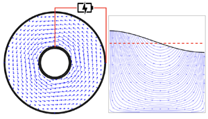
Inspired by these experiments, we consider an electromagnetically driven flow in an unsupported free film between two conducting coaxial cylindrical electrodes with radii $R_1$ and $R_2>R_1$ and placed in a vertical uniform magnetic field ${\boldsymbol {B}}=(0,0,B)$ as schematically shown in figure 2. The potential difference between the inner and outer electrodes is $V$.

Figure 2. The top (a) and side (b) views of the radial cross-section of an annular free film of electrically conducting fluid spanning the gap between two coaxial cylindrical electrodes with radii $R_1$ and $R_2>R_1$. The film is placed in a vertical uniform magnetic field ${\boldsymbol {B}}=(0,0,B)$. Electric current flowing through the film between the two electrodes generates a Lorentz force that drives the flow azimuthally.

In what follows we scale the radial coordinate $r$ with $R_2-R_1$, the film thickness $h$ with its average value $\langle h\rangle$ and choose the flow velocity scale in such a way that $\textit {Ca}\,\textit {Re}=1$ in (2.20a–d), that is, $U=\sqrt {\gamma \langle h\rangle /(\rho (R_2-R_1)^2)}$. With $B$ used as the magnetic field scaling, the Hartmann number becomes $\textit {Ha}^2=B^2(R_2-R_1)^2Kc_{b}^{(0)}/\mu$, where $c_b^{(0)}$ is the average solute concentration in the bulk. We scale the electric potential with voltage $V$ applied between the electrodes and introduce a new dimensionless parameter $W=Kc_{b}^{(0)}BV/(\rho U^2)$ that characterises the strength of the electric component $Kc_{b}^{(0)}BV/(R_2-R_1)$ of the Lorentz force acting on a unit volume of fluid relative to the radial pressure gradient $\rho U^2/(R_2-R_1)$. Parameter $W$ is similar to the Lorentz force parameter $Q=u_{lor}/u_{visc}$ introduced in Piedra et al. (Reference Piedra, Román, Figueroa and Cuevas2018), where $u_{lor}=Kc_{b}^{(0)}BV(R_2-R_1)/\mu$ is the characteristic velocity determined from the balance between the Lorentz force and viscous dissipation and $u_{visc}=\mu /(\rho (R_2-R_1))$ is the viscous velocity scale. Thus, in the scaling used here the effective Lorentz force parameter is given by $Q=\textit {Re}\,W=Kc_{b}^{(0)}BV (R_2-R_1)/(\mu U)$. It quantifies the ratio of $u_{lor}$ and the characteristic flow velocity scale $U$. Note that since $\textit {Re}\,\textit {Ca}=1$, the Lorentz force parameter can also be expressed as $Q=W/\textit {Ca}$. Scaling back to the physical variables we obtain

(3.1)\begin{equation} Q=\dfrac{Kc_{b}^{(0)}BV (R_2-R_1)^2}{\mu} \sqrt{\frac{\rho}{\gamma\langle h\rangle}}.\end{equation}

All other dimensionless parameters $\textit {Ma}$, $\textit {Ha}$, $\textit {Ca}$, $\textit {Pe}$ and $\textit {Sc}$ are obtained from (2.20a–d) by setting $L=R_2-R_1$. The dimensionless inner and outer radii are given by $\alpha$ and $1+\alpha$, respectively, where $\alpha =R_1/(R_2-R_1)$. The concentration of a surfactant is scaled using the average value $c_s^{(0)}$. Using the same symbols for non-dimensionless fields, we convert the invariant form of (2.47) to polar coordinates $(r,\theta )$ and obtain

(3.2)\begin{align} &\partial_tu_r +u_r\partial_ru_r+\frac{u_\theta}{r}\partial_\theta u_r-\frac{u_\theta^2}{r}\nonumber\\ &\quad =g(h)\partial_rh+\partial_r\left(\frac{\partial_rh}{r} +\partial_r^2h+\frac{\partial_\theta^2h}{r^2}\right)+\textit{Ca}\left(\frac{\partial_ru_r}{r}+\partial_r^2u_r +\frac{\partial_\theta^2u_r}{r^2}-\frac{u_r}{r^2}-\frac{2\partial_\theta u_\theta}{r^2}\right)\nonumber\\ &\qquad -\textit{Ca}\,\textit{Ha}^2u_r -{\textit{Ca}\,\textit{Q}} \frac{\partial_\theta\phi}{r}+\frac{\textit{Ca}}{h}V_r+3\,\textit{Ca}\,\partial_r\left(\frac{u_r}{r}+\partial_r u_r +\frac{\partial_\theta u_\theta}{r} \right) -\frac{\textit{Ca}\,\textit{Ma}}{\textit{Pe}}\frac{\partial_rc_s}{h}, \end{align}

(3.3)\begin{align} &\partial_tu_\theta + u_r\partial_ru_\theta+\frac{u_\theta}{r}\partial_\theta u_\theta +\frac{u_\theta u_r}{r}\nonumber\\ &\quad =\frac{1}{r}g(h)\partial_\theta h {\,+\,}\frac{1}{r}\partial_\theta\left(\frac{\partial_r h}{r}{\,+\,}\partial_{r}^2h {\,+\,}\frac{\partial_\theta^2h}{r^2}\right) +\textit{Ca}\left(\frac{\partial_ru_\theta}{r}{\,+\,}\partial_{r}^2u_\theta {\,+\,}\frac{\partial_{\theta}^2u_\theta}{r^2}{\,-\,}\frac{u_\theta}{r^2} {\,+\,}\frac{2\partial_\theta u_r}{r^2}\right)\nonumber\\ &\qquad +{\textit{Ca}\,\textit{Q}}\partial_r \phi +\frac{\textit{Ca}}{h}V_\theta-\textit{Ca}\,\textit{Ha}^2u_\theta +\frac{3\,\textit{Ca}}{r}\partial_\theta\left(\frac{u_r}{r}+\partial_r u_r +\frac{\partial_\theta u_\theta}{r} \right) -\frac{\textit{Ca}\,\textit{Ma}}{\textit{Pe}}\frac{\partial_\theta c_s}{hr}, \end{align}

with

(3.4)\begin{align} V_r&=2\left(\partial_rh\partial_ru_r +\frac{1}{r^2}\partial_\theta h\partial_\theta u_r -\frac{1}{r^2}u_\theta\partial_\theta h\right) +\frac{1}{r^2}(\partial_r[ru_\theta] -\partial_\theta u_r)\partial_\theta h\nonumber\\ &\quad +\frac{2}{r}(\partial_r[ru_r]+\partial_\theta u_\theta)\partial_r h, \end{align}

(3.5)\begin{align} V_\theta&=2\left(\partial_rh\partial_ru_\theta +\frac{1}{r^2}\partial_\theta h\partial_\theta u_\theta +\frac{1}{r^2}u_r\partial_\theta h\right) -\frac{1}{r}(\partial_r[ru_\theta]-\partial_\theta u_r)\partial_r h\nonumber\\ &\quad +\frac{2}{r^2}(\partial_r[ru_r] +\partial_\theta u_\theta)\partial_\theta h. \end{align}

The dynamic equations for the salt and surfactant concentrations and the kinematic condition are given by

(3.6)$$\begin{gather} \partial_t[hc_b]+\frac{1}{r}(\partial_r[rhc_bu_r]+\partial_\theta[hc_bu_\theta]) =\frac{\textit{Sc}^{-1}\,\textit{Re}^{-1}}{r^2}[r\partial_r[rh\partial_rc_b]+\partial_\theta[h\partial_\theta c_b]], \end{gather}$$

(3.7)$$\begin{gather}\partial_t c_s+\frac{1}{r}(\partial_r[rc_su_r]+\partial_\theta[c_su_\theta]) =\frac{\textit{Pe}^{-1}}{r^2}[r\partial_r[r\partial_rc_b]+\partial_\theta^2c_s], \end{gather}$$

(3.8)$$\begin{gather}\partial_th+\frac{1}{r}(\partial_r[rhu_r]+\partial_\theta[hu_\theta])=0. \end{gather}$$

The system is completed by the continuity equation for the electric current

(3.9)\begin{equation} \partial_r[c_brh({\textit{Ca}\,\textit{Ha}^2} u_\theta-{\textit{Ca}\,\textit{Q}}\partial_r\phi)] -\partial_\theta\left[\frac{c_bh}{r}({\textit{Ca}\,\textit{Ha}^2} ru_r +{\textit{Ca}\,\textit{Q}}\partial_\theta\phi)\right]=0.\end{equation}

The system of equations (3.3)–(3.9) admits a steady solution that corresponds to the azimuthal flow field $u_r=0$, $u_\theta =f(r)$ induced by axisymmetric electric potential $\phi (r)$ in a film with axisymmetric profile $h(r)$ containing uniformly dissolved salt with constant bulk concentration $c_b=1$ and covered by a uniformly distributed surfactant with a surface concentration $c_s=1$. In what follows we study the properties and linear stability of the base azimuthal flow field, the instability of which determines the onset of the secondary possibly non-axisymmetric finite-amplitude flows.

The functions $f(r)$, $h(r)$ and $\phi (r)$ are found from

(3.10)$$\begin{gather} \left(\dfrac{(rh')'}{r}\right)'+g(h)h'+\dfrac{f^2}{r}=0, \end{gather}$$

(3.11)$$\begin{gather}f''+\dfrac{f'}{r}-\dfrac{f}{r^2}-\textit{Ha}^2\,f+{\textit{Q}}\phi' +\dfrac{h'}{h}\left(\,f'-\dfrac{f}{r}\right)=0, \end{gather}$$

(3.12)$$\begin{gather}(r h({\textit{Q}}\phi'-{\textit{Ha}^2}\,f))'=0, \end{gather}$$

where primes denote the radial derivative ${\textrm {d}}/{\textrm {d}r}$.

Equation (3.12) is integrated once to yield

(3.13)\begin{equation} \phi'={\frac{\textit{Ha}^2}{\textit{Q}}}f-\frac{e}{rh},\end{equation}

where constant $e$ is linked to the potential difference $\phi (1+\alpha )-\phi (\alpha )={1}$ between the electrodes via

(3.14)\begin{equation} {1=\frac{\textit{Ha}^2}{Q}}\int_\alpha^{1+\alpha}f(r)\,\textrm{d}r-e \int_\alpha^{1+\alpha}\frac{\textrm{d}r}{rh}.\end{equation}

The term $e/(rh)$ in (3.13) is related to the radial current density

(3.15)\begin{equation} j_r={\textit{Ca}\,\textit{Ha}^2}f-{\textit{Ca}\,\textit{Q}}\phi'=\frac{{\textit{Ca}\,\textit{Q}}e}{rh}. \end{equation}

The total steady current through the vertical cylindrical section of the film at any radial location $\alpha \leq r\leq 1+\alpha$ is independent of the radius of a cross-section and is given by $4{\rm \pi} rhj_r=4{\rm \pi} \,{\textit {Ca}\,\textit {Q}}e$.

Eliminating $\phi$ from (3.11), we obtain two coupled equations for $f$ and $h$,

(3.16)$$\begin{gather} \left(\dfrac{(rh')'}{r}\right)'+g(h)h'+\dfrac{f^2}{r}=0, \end{gather}$$

(3.17)$$\begin{gather}f''+\dfrac{f'}{r}-\dfrac{f}{r^2}-{\textit{Q}}\dfrac{e}{rh} +\dfrac{h'}{h}\left(\,f'-\dfrac{f}{r}\right)=0. \end{gather}$$

Fluid velocity vanishes at the surface of the electrodes leading to $f(\alpha )=f(1+\alpha )=0$. The boundary condition for the film deformation must be compatible with the long-wave approximation used here, which only takes into account relatively small film slopes $h'\ll 1$. In what follows we assume that $h'(\alpha )=h'(1+\alpha )=0$.

We are looking for a solution of the boundary value problems (3.16) and (3.17) that corresponds to a given average film half-thickness

(3.18)\begin{equation} \frac{2}{1+2\alpha}\int_{\alpha}^{1+\alpha }h(r)r\,\textrm{d}r=1 \end{equation}

and satisfies the additional integral condition (3.14) for any given value of the applied voltage $V$ that only appears in the definition of parameter $\textit {Q}$.

For reference, we derive the approximate analytic solution that corresponds to the flow in a flat undeformed film. By setting $h=1$ and neglecting the centrifugal acceleration $f^2/r$, we find from (3.17) and (3.14) that

(3.19)\begin{equation} f={\alpha e\textit{Q}} \left[C\left(\frac{\alpha}{r}-\frac{r}{\alpha}\right) +\frac{r}{2\alpha}\ln\frac{r}{\alpha}\right]\!,\end{equation}

where

(3.20)\begin{equation} \left.\begin{gathered} C=\dfrac{(1+\alpha)^2\ln{(1+\alpha^{-1})}}{2(1+2\alpha)},\quad e=\dfrac{{1}}{\alpha^2\,\textit{Ha}^2D-\ln(1+\alpha^{-1})},\\ D=C\ln\left(1+\alpha^{-1}\right)-\dfrac{1+2\alpha}{8\alpha^2}. \end{gathered}\right\} \end{equation}

To find non-trivial solutions of the boundary value problem (3.16), (3.17) with the integral condition (3.18), we use a numerical continuation package AUTO (Doedel et al. Reference Doedel, Wang and Fairgrieve1994; Krauskopf et al. Reference Krauskopf, Osinga and Galan-Vioque2014). The trivial solution $f=0$ and $h=1$ that exists for $\textit {Q}=0$ is used as a starting point for numerical continuation with $\textit {Q}$ being gradually increased.

In the absence of the disjoining pressure, that is, for $g(h)=0$, the boundary value problem (3.16), (3.17), (3.14), (3.18) has an important scaling property. Namely, it contains three dimensionless parameters, $\textit {Ha}$, $\alpha$ and the Lorentz force parameter $\textit {Q}$, but only $\textit {Q}$ depends explicitly on the dimensional layer thickness $2\langle h\rangle$. This implies that, for any fixed $\textit {Ha}$ and $\alpha$, there exists a universal branch of solutions parameterised by (3.1). A solution that corresponds to an arbitrary value of the average film half-thickness $\langle h\rangle$ and an arbitrary applied voltage $V$ is found on the universal branch for the corresponding value of $\textit {Q}$.

Taking into account the above scaling property we consider a free film with an arbitrary average half-thickness $\langle h\rangle$ spanning the gap between cylindrical electrodes with radii $R_1=1$ cm and $R_2=2$ cm ($\alpha =1$). As an example, we chose fluid properties and a magnetic field strength similar to those used in Pérez-Barrera et al. (Reference Pérez-Barrera, Ortiz and Cuevas2016) and Suslov et al. (Reference Suslov, Pérez-Barrera and Cuevas2017): $Kc_b^{(0)}=\sigma =5\ (\textrm {Ohm}\ \textrm {m})^{-1}$, $\mu =0.001\ \textrm {kg}\ \textrm {m}\ \textrm {s}^{-1}$, $\rho =1000\ \textrm {kg}\ \textrm {m}^{-3}$, $B=0.05\ \textrm {T}$. Additionally, we use $\gamma =0.03\ \textrm {N}\ \textrm {m}^{-1}$ for the surface tension coefficient. These correspond to $\textit {Ha}^2\approx 1.3\times 10^{-3}$. As the solution measure, we take the maximum flow velocity $f_{max}$ and the minimum film thickness $h_{min}$ attained at the inner cylinder ($r=\alpha$). The numerically obtained maximum velocity $f_{max}$ is shown in figure 3(a) by the solid line while the value found from the flat-film approximation (3.19) is depicted by the dashed line. The minimum film thickness is shown in the log-log scale in figure 3(b) indicating that $h_{min}$ asymptotically approaches zero as a power law function ${\sim }{\textit {Q}}^{-2.4}$. This implies that the solution exists for any fixed value of ${\textit {Q}}$ no matter how large it is. However, the film thickness becomes vanishingly small at the inner electrode indicating that the film is likely to rapture there.

Figure 3. (a) Maximum fluid velocity in a free annular film as a function of the Lorentz force parameter $\textit {Q}$ for $\textit {Ha}^2=1.3\times 10^{-3}$ and $\alpha =1$. The dashed and solid lines correspond to the flat-film approximation (3.19) and the numerical solution, respectively. (b) Minimum film thickness $h_{min}$ at the inner cylinder as a function of the applied voltage. The dashed line depicts the power law function ${\sim }({\textit {Q}})^{-2.4}$. (c) Film thickness $h(r)$ for the values of $\Delta \phi$ at points $1$ and $2$ labelled in panel (a). (d) Velocity $f(r)$ for solutions at points $1$ and $2$ in panel ($a$) (solid lines) and corresponding to the flow in the flat-film approximation (3.19) (dashed lines).

We also emphasise that all results presented in this paper are obtained by neglecting the disjoining pressure. This introduces a natural limitation on their applicability for films that are thinner than approximately 100 nm. For example, if $\langle h\rangle =10\ \mathrm {\mu }\textrm {m}$ as in figures 5 and 6 in § 4, the smallest dimensionless film thickness $h_{min}=10^{-7}\ \textrm {m}/\langle h\rangle$ for which the presented results are expected to remain valid is $h_{min}\approx 10^{-2}$, that is, about 1 % of the average film thickness.

The film profile and the flow velocity at points $1$ and $2$ are shown in figures 3(c) and 3(d), respectively. The dashed line in figure 3(d) corresponds to the approximate solution (3.19).

4. Linear stability of the azimuthal flow

In this section we study the linear stability of the base azimuthal flow $(u_r,u_\theta )=(0,f(r))$ in a free film with the half-thickness $h_0(r)$ in the absence of the disjoining pressure ($\varPi (h)=0$). It is anticipated that the least stable perturbations are azimuthally invariant due to the stabilising effect of the surface tension. Indeed, any perturbation that varies azimuthally must be periodic in $\theta$ and, consequently, be proportional to $\textrm {e}^{\textrm {i} n\theta }$, $n=0,1,2,\ldots\ $. Therefore, the magnitude of the stabilising surface tension terms in (3.3) increases as $n^3$ and is the smallest for $n=0$.

Equations (3.3)–(3.9) are linearised about the base flow by writing

(4.1)\begin{equation} \left.\begin{gathered} u_r={\rm e}^{\lambda t}{\tilde{u}}_r(r),\quad u_\theta=f(r)+{\rm e}^{\lambda t}{\tilde{u}}_\theta(r), \quad h=h_0+{\rm e}^{\lambda t}{\tilde{h}},\\ c_b=1+{\rm e}^{\lambda t}{\tilde{c}}_b,\quad c_s=1+{\rm e}^{\lambda t}{\tilde{c}}_s,\quad \phi'={\dfrac{\textit{Ha}^2}{\textit{Q}}}f-\dfrac{e}{rh_0} +{\rm e}^{\lambda t}{\tilde{\phi}}'(r), \end{gathered}\right\}\end{equation}

where $\lambda$ is the perturbation growth rate, $h_0=h_0(r)$ is the steady film profile and the tilded variables represent small-amplitude perturbations, substituting these in the equations and neglecting the products of perturbations. After dropping the tildes we obtain

(4.2)$$\begin{gather} \lambda u_r =-\frac{2fu_\theta}{r} +\left(\frac{(rh')'}{r}\right)'+4\,\textit{Ca}\left(\frac{(ru_r)'}{r}\right)' -\textit{Ca}\,\textit{Ha}^2u_r\nonumber\\ \quad +\frac{2\,\textit{Ca}\, h_0'}{h_0}\left(\frac{u_r}{r}+2u_r'\right) -\frac{\textit{Ca}\,\textit{Ma}}{\textit{Pe} h_0} c'_s, \end{gather}$$

(4.3)$$\begin{gather} \lambda u_\theta=-u_rf'-\frac{fu_r}{r}+\textit{Ca}\left(\frac{(ru_\theta)'}{r}\right)' -{\textit{Ca}\,\textit{Ha}^2 u_\theta+\textit{Ca}\,\textit{Q}\phi'}\nonumber\\ \quad +\frac{\textit{Ca}\, h_0'}{h_0}\left(u_\theta'-\frac{u_\theta}{r}\right) +\textit{Ca}\left(\frac{h}{h_0}\right)'\left(\,f'-\frac{f}{r}\right)\!, \end{gather}$$

(4.4)$$\begin{gather} \lambda h=-\frac{1}{r}\left(rh_0u_r\right)', \end{gather}$$

(4.5)$$\begin{gather}\lambda c_bh_0+\lambda h=-\frac{1}{r}(rh_0u_r)' +\textit{Sc}^{-1}\,\textit{Re}^{-1}\frac{(rh_0(c_b)')'}{r}, \end{gather}$$

(4.6)$$\begin{gather}\lambda c_s=-\frac{1}{r}\left(ru_r\right)' +\textit{Pe}^{-1}\frac{(r(c_s)')'}{r}, \end{gather}$$

(4.7)$$\begin{gather}0=\left(rh_0\left( {\dfrac{\textit{Ha}^2}{\textit{Q}}} u_\theta-\phi'\right)\right)' +\left(\frac{e\left( h+c_b h_0\right)}{ h_0}\right)'. \end{gather}$$

The flow velocity vanishes at $r=\alpha$ and $r=1+\alpha$ so that $u_r=u_\theta =0$ there. This leads to the automatic conservation of the total volume of the fluid

(4.8)\begin{equation} \int_\alpha^{1+\alpha}2{\rm \pi} hr\,\textrm{d}r=-\frac{1}{\lambda}\int_\alpha^{1+\alpha} \frac{2{\rm \pi}}{r}\left(rh_0u_r\right)'r\,\textrm{d}r=0.\end{equation}

To describe moving contact lines at the surface of the electrodes, we assume that the dynamic contact angle is equal to its static value at all times, that is, we require that $h'(\alpha )=h'(1+\alpha )=h_0'(\alpha )=h_0'(1+\alpha )=0$. The case of the dynamically changing contact angle and non-zero wetting line friction will be considered in future studies. Differentiating (4.4) and applying the conditions and $u_r(\alpha )=u_\theta (\alpha )=u_r(1+\alpha )=u_\theta (1+\alpha )=0$ we obtain two additional boundary conditions for the radial velocity $u_r$,

(4.9)\begin{equation} u_r'(\alpha)+u_r''(\alpha) =\frac{u_r'(1+\alpha)}{1+\alpha}+u_r''(1+\alpha)=0.\end{equation}

Integrating the equation for the perturbation of the electric potential (4.7) once we obtain

(4.10)\begin{equation} {\dfrac{\textit{Ha}^2}{\textit{Q}}}u_\theta-\phi'=\frac{c}{rh_0}-\frac{eh}{rh_0^2} -\frac{ec_b}{rh_0},\end{equation}

where $c$ is some constant. Integrating (4.10) and imposing the condition $\phi (\alpha )=\phi (1+\alpha )=0$ we find that

(4.11)\begin{equation} {\dfrac{\textit{Ha}^2}{\textit{Q}}}\int_\alpha^{1+\alpha}u_\theta\,\textrm{d}r =c\int_\alpha^{1+\alpha}\frac{\textrm{d}r}{rh_0} -e\int_\alpha^{1+\alpha}\frac{h}{rh_0^2}\textrm{d}r -e\int_\alpha^{1+\alpha}\frac{c_b}{rh_0}\textrm{d}r.\end{equation}

Multiplying (4.2) and (4.3) by $\lambda$, using (4.4) and (4.10) to eliminate $h$ and $\phi '$ and, subsequently, differentiating (4.5) and (4.6) with respect to the radius $r$ we arrive at a nonlinear eigenvalue problem,

(4.12)\begin{align} \lambda^2 u_r-\frac{2\lambda fu_\theta}{r} &=-\left(\frac{(r(r^{-1}\left(rh_0u_r\right)')')'}{r}\right)' +4\lambda\,\textit{Ca}\left(\frac{(ru_r)'}{r}\right)' -\lambda \,\textit{Ca}\,\textit{Ha}^2u_r\nonumber\\ &\quad +\frac{2\,\textit{Ca}\,\lambda h_0'}{h_0}\left(\frac{u_r}{r}+2u_r'\right) -\frac{\textit{Ca}\,\textit{Ma}}{\textit{Pe}}\frac{\lambda c_s'}{h_0}, \end{align}

(4.13)\begin{align} \lambda^2 u_\theta+\lambda u_rf' &=-\frac{\lambda fu_r}{r} +\lambda\,\textit{Ca}\left(\frac{(ru_\theta)'}{r}\right)' -{\textit{Ca}\,\textit{Q}}\left(\frac{e (rh_0 u_r)'}{r^2h_0^2} -\frac{\lambda e c_b}{rh_0}+\frac{\lambda c}{rh_0}\right)\nonumber\\ &\quad +\frac{\lambda\,\textit{Ca}\, h_0'}{h_0} \left(u_\theta'-\frac{u_\theta}{r}\right) -\textit{Ca}\left(\frac{(rh_0u_r)'}{rh_0}\right)'\left(\,f'-\frac{f}{r}\right)\!, \end{align}

(4.14)\begin{align} \lambda c_b'&=\textit{Sc}^{-1}\,\textit{Re}^{-1}\left(\frac{(rh_0c_b')'}{rh_0}\right)',\end{align}

(4.15)\begin{align} \lambda c_s' &= \textit{Pe}^{-1}\left(\frac{(rc_s')'}{r}\right)' -\left(\frac{\left(ru_r\right)'}{r}\right)'\end{align}

that must be solved in conjunction with the integral condition (4.11). The set of boundary conditions (4.9) and $u_r(\alpha )=u_\theta (\alpha )=u_r(1+\alpha )=u_\theta (1+\alpha )=0$ must be extended with

(4.16)\begin{equation} c_s'(\alpha)=c_b'(\alpha)=c_s'(1+\alpha)=c_b'(1+\alpha)=0,\end{equation}

which accounts for the chemically passive impenetrable boundaries of the two electrodes. Note that unlike (3.16) and (3.17) the eigenvalue problem (4.15) contains the average film thickness $\langle h\rangle$ as a part of the capillary number $\textit {Ca}$.

4.1. Linear stability of a flat film with no applied voltage

In this section we consider the stability of a flat film in the absence of an electric current. With $h_0=1$, $f=0$ and $e=0$ the eigenvalue problem (4.12)–(4.15) and the integral condition (4.11) reduce to three decoupled eigenvalue problems: one for the azimuthal velocity perturbations $u_\theta$, one for the radial velocity $u_r$ and surfactant $c_s$ perturbations and one for the perturbation of the solute concentration $c_b$:

(4.17)$$\begin{gather} \lambda u_\theta =\textit{Ca}\,\mathcal{L}\{u_\theta\} -\frac{\textit{Ca}\,\textit{Ha}^2}{r\ln\left(1+\alpha^{-1}\right)} \int_\alpha^{1+\alpha}u_\theta\,\textrm{d}r, \end{gather}$$

(4.18)$$\begin{gather}\lambda^2 u_r =- \mathcal{L}\{\mathcal{L}\{u_r\}\}+4\lambda\textit{Ca}\,\mathcal{L}\{u_r\} -\lambda\textit{Ca}\,\textit{Ha}^2u_r-\textit{Ca}\,\textit{Ma}\,\textit{Pe}^{-1}\lambda c_s', \end{gather}$$

(4.19)$$\begin{gather}\lambda c_s'=\textit{Pe}^{-1}\,\mathcal{L}\{c_s'\} -\mathcal{L}\{u_r\}, \end{gather}$$

(4.20)$$\begin{gather}\lambda c_b'=\textit{Sc}^{-1}\,\textit{Re}^{-1}\mathcal{L}\{c_b'\}. \end{gather}$$

Here $\mathcal{L}\{u\}\equiv (r^{-1}(ru)')'$.

The eigenvalue problem (4.17)–(4.20) can be solved analytically in terms of the auxiliary eigenvalue problem for the operator $\mathcal {L}$,

(4.21)\begin{equation} \mathcal{L}\{u\}=-\varLambda u,\end{equation}

which coincides with Bessel's differential equation. The solution of (4.21) that satisfies the Dirichlet boundary conditions $u(\alpha )=u(1+\alpha )=0$ exists only for real positive $\varLambda$ and is given by

(4.22)\begin{equation} u(r)=C_1 {\rm J}_1\left(r\sqrt{\varLambda}\right) +C_2{\rm Y}_1\left(r\sqrt{\varLambda}\right)\!,\end{equation}

where $C_1$ and $C_2$ are arbitrary constants and $\textrm {J}_1$ and $\textrm {Y}_1$ are the Bessel functions of order one of the first and second kind, respectively. Applying the boundary conditions we obtain the solvability condition for constants $C_1$ and $C_2$ that determines the entire spectrum of discrete eigenvalues $\varLambda$,

(4.23)\begin{equation} {\rm J}_1\left(\alpha\sqrt{\varLambda}\right) {\rm Y}_1\left((1+\alpha)\sqrt{\varLambda }\right) -{\rm J}_1\left((1+\alpha)\sqrt{\varLambda}\right) {\rm Y}_1\left(\alpha\sqrt{\varLambda}\right)=0.\end{equation}

It follows from (4.21)–(4.23) that the spectrum of eigenvalues $\lambda _{c_b}$ of the bulk solute concentration perturbations (4.20) is real and negative, i.e.

(4.24)\begin{equation} \lambda_{c_b}=-(\textit{Sc}\,\textit{Re})^{-1}\varLambda,\end{equation}

and the corresponding eigenfunction is given by

(4.25)\begin{equation} c_b'(r)=C\left[ {\rm J}_1\left(r\sqrt{\varLambda}\right) {\rm Y}_1\left(\alpha\sqrt{\varLambda}\right) -{\rm Y}_1\left(r\sqrt{\varLambda}\right) {\rm J}_1\left(\alpha\sqrt{\varLambda}\right)\right]\!,\end{equation}

where $C$ is an arbitrary constant.

The eigenvalue problem (4.18) and (4.19) for $u_r$ and $c_s'$ can be solved in a similar way using the eigenfunctions of the operator $\mathcal {L}$. The solution that satisfies $u_r(\alpha )=u_r(1+\alpha )=0$ and $c_s'(\alpha )=c_s'(1+\alpha )=0$ is given by

(4.26)\begin{equation} \left.\begin{gathered} u_r(r) =C_1\left[ {\rm J}_1\left(r\sqrt{\varLambda}\right) {\rm Y}_1\left(\alpha\sqrt{\varLambda}\right) -{\rm Y}_1\left(r\sqrt{\varLambda}\right) {\rm J}_1\left(\alpha\sqrt{\varLambda}\right)\right]\!,\\ c_s'(r) =C_2u_r, \end{gathered}\right\}\end{equation}

where $C_1$ and $C_2$ are some constants.

Substituting (4.26) into (4.18) and (4.19) we obtain

(4.27)$$\begin{gather} \lambda^2=-\varLambda^2-\textit{Ca}(4\varLambda+\textit{Ha}^2)\lambda-C_2\,\textit{Ca}\,\textit{Ma}\,\textit{Pe}^{-1}\lambda, \end{gather}$$

(4.28)$$\begin{gather}\lambda C_2=\varLambda-\textit{Pe}^{-1}\varLambda C_2, \end{gather}$$

and then eliminating $C_2$ from (4.27) we arrive at a cubic equation for $\lambda$,

(4.29)\begin{equation} (\textit{Pe}\,\lambda+\varLambda)(\lambda^2 +\textit{Ca}(4\varLambda+\textit{Ha}^2)\lambda+\varLambda^2) +b\varLambda\lambda\,\textit{Pe}=0,\end{equation}

where $b=\textit {Ca}\,\textit {Ma}\,\textit {Pe}^{-1}>0$ characterises the strength of the Marangoni flow.

For any admissible value of $\varLambda$ from (4.23), one needs to solve (4.29) to find the eigenvalue $\lambda$. Then the corresponding eigenfunctions (4.26) only contain one arbitrary scaling factor $C_1$ with $C_2=\varLambda /(\lambda +\textit {Pe}^{-1}\varLambda )$. Here we consider two physically distinct situations: the diffusion-dominated regime, when the surface diffusivity is large, i.e. $d_s\to \infty$, and the advection-dominated regime, when $d_s\to 0$. Since the Hartmann number $\textit {Ha}$, the capillary number $\textit {Ca}$ and parameter $b=\textit {Ca}\,\textit {Ma}\,\textit {Pe}^{-1}$ in (4.29) do not depend on $d_s$, the diffusion-dominated regime corresponds to $\textit {Pe}\to 0$ with $\textit {Ha}$, $\textit {Ca}$ and $b$ remaining finite. In this case (4.29) has three distinct solutions:

(4.30)$$\begin{gather} \lambda_{1,2}=-\frac{\textit{Ca}\left(4\varLambda+\textit{Ha}^2\right)+b\,\textit{Pe}}{2} \pm\frac{\varOmega}{2}\left(1+b\,\textit{Pe}\frac{\textit{Ca}(4\varLambda+\textit{Ha}^2)} {2\varOmega^2}\right)+O(\textit{Pe}^2), \end{gather}$$

(4.31)$$\begin{gather}\lambda_3=-\textit{Pe}^{-1}\varLambda+b\,\textit{Pe}+O(\textit{Pe}^2). \end{gather}$$

Here $\varOmega =\sqrt {\textit {Ca}^2(4\varLambda +\textit {Ha}^2)^2-4\varLambda ^2}$.

Note that $\lambda _3$ is real and negative and its magnitude is always much larger than $|\lambda _{1,2}|$. Since $\varLambda$ is real and positive, we conclude that the real parts of $\lambda _{1,2}$ are always negative. Moreover, $\lambda _{1,2}$ become complex if $\textit {Ca}(4\varLambda +\textit {Ha}^2)<2\varLambda$ implying that the radial perturbation mode undergoes the transition from a monotonic to oscillatory decay. In physical variables, the condition for the oscillatory decay of the radial mode is

(4.32)\begin{equation} \sqrt{\rho\gamma\langle h\rangle}> 2\mu+\frac{B^2 (R_2-R_1)^2\sigma}{2\varLambda},\end{equation}

where the electric conductivity is $\sigma =Kc_b^{(0)}$ and $\varLambda$ depends on the ratio of the radii $R_2/R_1$ via parameter $\alpha$. It is instructive to compare condition (4.32) with the linear stability of an unbounded flat free layer in the absence of the magnetic field. Neglecting the disjoining pressure, the growth rate $\omega (k)$ of the least stable mode with the wavenumber $k$ in an unbounded horizontal free film can be obtained from (30) in Erneux & Davis (Reference Erneux and Davis1993):

(4.33)\begin{equation} \frac{\mu}{\rho}\omega(k)=-2k^2 +k^2\sqrt{4-\frac{\rho\langle h\rangle\gamma}{\mu^2}}. \end{equation}

It follows from (4.33) that the critical thickness $2\langle h\rangle _c$ of the layer above which the relaxation dynamics is oscillatory is given by

(4.34)\begin{equation} 2\langle h\rangle_c=\frac{8\mu^2}{\rho\gamma}.\end{equation}

This coincides with our result (4.32) for $B=0$.

It is seen from (4.30) that in the absence of the Marangoni flow, that is, when $b=0$, the eigenvalue of the radial velocity perturbation with the largest real part is given by

(4.35)\begin{equation} \lambda_1=-\frac{\textit{Ca}\left(4\varLambda+\textit{Ha}^2\right)}{2} +\frac{\varOmega}{2}.\end{equation}

The perturbation of the surfactant is decoupled from that of the radial flow and has a negative real eigenvalue $\lambda _3=-\varLambda \,\textit {Pe}^{-1}$. In this regime, any perturbation of the surfactant distribution relaxes on the time scale $|\lambda _3|^{-1}$, which is much shorter than the characteristic decay time $-{\rm Re} ({\lambda _{1,2}}^{-1})$ of fluid motion. In the presence of the Marangoni flow when $b\ne 0$, the perturbations of the radial velocity and surfactant concentrations are coupled and their dynamics is characterised by the leading eigenvalues $\lambda _{1,2}$. The Marangoni flow leads to a further stabilisation of the leading perturbation mode as follows from (4.30). Indeed, by analysing the real parts of the leading eigenvalues we conclude that

(4.36)\begin{equation} {\rm Re}(\lambda_{1,2})|_{b>0}<{\rm Re}(\lambda_{1,2})|_{b=0}<0 \end{equation}

regardless of the sign of $\varOmega ^2$. As a consequence, the characteristic decay time of the flow perturbation decreases in the presence of the Marangoni effect.

As follows from (4.19), in the advection-dominated regime $\textit {Pe}\to \infty$ the dynamics of the surfactant perturbation is governed by the radial flow $u_r$. Indeed in this limit $\lambda c_s'=-\mathcal{L}\{u_r\}$, which shows that the surfactant plays the role of an active scalar field advected by the flow while its gradient influences the stability of the flow. By letting $\textit {Pe}\to \infty$ in (4.28) and then substituting $C_2=\varLambda /\lambda$ in (4.27) we obtain

(4.37)\begin{equation} \lambda_{{\pm}}\approx\tfrac{1}{2}\left[-\textit{Ca}\left(4\varLambda+\textit{Ha}^2\right) \pm\sqrt{\textit{Ca}^2\left(4\varLambda+\textit{Ha}^2\right)^2 -4\varLambda(\varLambda+b)}\right].\end{equation}

From (4.37) we see that the Marangoni flow has no effect on the stability of the base flow if the expression under the radical is negative. However, if

(4.38)\begin{equation} \textit{Ca}^2\left(4\varLambda+\textit{Ha}^2\right)^2-4\varLambda(\varLambda+b)>0, \end{equation}

the leading eigenvalue $\lambda _+$ becomes real and negative, and the presence of surfactant has a stabilising effect since $|\lambda _+|_{b>0}>|\lambda _+|_{b=0}$. These analytical results extend an earlier study on the linear stability of planar soap films (Miksis & Ida Reference Miksis and Ida1998) by including the Lorentz force effects. The observation of the stabilising role of the Marangoni flow in the limit of diffusion-dominated and advection-dominated regimes is in agreement with Miksis & Ida (Reference Miksis and Ida1998), where it was also found that for long-wavelength perturbations the presence of the Marangoni flow decreases the growth rate of the dominant perturbation mode.

To illustrate the structure of the oscillatory radial mode, we consider the diffusion-dominated regime in a film with the average thickness $2\langle h\rangle =20\ \mathrm {\mu }\textrm {m}$ and take all other parameters as in figure 3. For $\alpha =1$, the leading eigenvalue of the operator $\mathcal {L}$ is $\varLambda \approx 10.218$, which corresponds to the complex leading eigenvalue of the radial mode $\lambda _r\approx -1.179\pm 10.149\textrm {i}$. The corresponding eigenfunction $u_r$ is shown in figure 4(a). Figure 4(b) depicts the instantaneous streamlines of the corresponding flow field in a vertical cross-section of the film $(r,z)$. The streamlines are obtained by recalling that the vertical flow velocity $w$ is given by $w(r,z)=-r^{-1}(ru_r)'z$ so that the kinematic equation (4.4) can be written in the form $\partial _t h =-w(r,1)=- r^{-1}(ru_r)'$. The film interface oscillates about $h_0=1$ with a decreasing amplitude while the fluid flows from the inner to the outer cylinder and back.

Figure 4. (a) Leading eigenfunction $u_r=\textrm {Y}_1(\alpha \sqrt {\varLambda }) \textrm {J}_1(r\sqrt {\varLambda }) -\textrm {J}_1(\alpha \sqrt {\varLambda }) \textrm {Y}_1(r\sqrt {\varLambda })$ of the radial perturbation mode for the same parameters as in figure 3 and $\langle h\rangle =10 \ \mathrm {\mu }\textrm {m}$. (b) Streamlines of the radially perturbed flow field in a vertical cross-section of the film.

Figure 5. (a) Real part of the first three leading eigenvalues as a function of the value of $\textit {Q}$ for the same parameters as in figure 3. The solid (dashed) lines correspond to complex (purely real) eigenvalues, respectively. Labels BP and NS mark the loci of the branching point of the azimuthal velocity mode and the point of neutral stability of the radial velocity mode, respectively; (b) the relative strength of the radial to azimuthal velocity mode $\chi$; (c) the neutrally stable film profile at point NS in panel (a); (d) the azimuthal velocity $f_0$ in a neutrally stable film; the magnitudes of the neutrally stable radial (e) and azimuthal (f) velocity perturbations.

It is instructive to consider the limit of a vanishingly small inner radius, that is, $\alpha \to 0$. Using the asymptotic expressions for the Bessel functions, $\textrm {J}_1(x)\approx x/2$ and $\textrm {Y}_1(x)\approx -2/({\rm \pi} x)$, as $x\to 0$, it can be shown that the leading eigenvalue $\varLambda$ from (4.23) is finite and is given by the first non-zero root of $\textrm {J}_1(\sqrt {\varLambda })=0$, that is, $\varLambda =3.8317^2=14.6819$. For $\langle h\rangle =10\ \mathrm {\mu }\textrm {m}$, this corresponds to a complex eigenvalue of the radial mode $\lambda _r=-1.695\pm {\rm i} 14.584$. The eigenfunction $u_r$ from (4.26) has a removable singularity at $r\to \alpha \to 0$ and its shape is similar to that of $u_r$ shown in figure 4(a). Therefore, in the absence of the applied voltage, the leading radially symmetric oscillation mode in a circular unsupported free film is a damped rocking mode with the shape as in figure 4(b).

The eigenvalue problem (4.17) for the azimuthal velocity perturbation $u_\theta$ can only be found analytically for a weak magnetic field at $\textit {Ha}\to 0$. When $\textit {Ha}=0$, the spectrum of the azimuthal velocity perturbations is real and is given by

(4.39)\begin{equation} \lambda_{u_\theta}=-\varLambda\,\textit{Ca}.\end{equation}

Comparing (4.39) with (4.30) we observe that in the absence of the Marangoni flow ($b=0$) and when $\textit {Ha}=0$, the absolute value of the eigenvalue $|\lambda _{u_\theta }|$ of the monotonically stable azimuthal velocity perturbation is exactly half of the real part of the eigenvalue $\lambda _{u_r}$ of the radial velocity mode.

4.2. Linear stability of a deformed film in the presence of electric current

In this section we study the linear stability of the azimuthal flow in a deformed film in the diffusion-dominated regime, when perturbations of the surfactant and solute fields relax instantaneously. The azimuthal and radial velocity perturbation modes discussed in the previous section become coupled in the presence of an electric current. This implies that, for any infinitesimal value of $\textit {Q}$, the spectrum of the generalized eigenvalue problem (4.15) is discrete and contains the eigenvalues that originate from each of the possible radial and azimuthal velocity modes existing in the absence of current.

To visualise how the stability of the azimuthal flow changes with the applied voltage, we choose $\langle h\rangle =10\ \mathrm {\mu }\textrm {m}$ and keep all other parameters as in figure 3. The numerical continuation method is then employed to track each mode and the corresponding eigenvalue using the value of $\textit {Q}$ as the continuation parameter. To this end, the generalized eigenvalue problem (4.15) is solved simultaneously with (3.16) and (3.17). To quantify the relative coupling strength between the perturbations of the radial and the azimuthal velocity, we introduce the parameter

(4.40)\begin{equation} \chi=\arctan{\left(\frac{\displaystyle\int\nolimits_\alpha^{1+\alpha}|u_r|^2\,\textrm{d}r} {\displaystyle\int\nolimits_\alpha^{1+\alpha}|u_\theta|^2\,\textrm{d}r}\right)}.\end{equation}

Thus, $\chi ={\rm \pi} /2$ corresponds to the pure radial and $\chi =0$ to pure azimuthal modes, respectively.

The real parts of the first three leading eigenvalues labelled by $r_1$, $\theta _1$ and $\theta _2$ are shown in figure 5(a). At $\textit {Q}=0$ the leading mode is the azimuthal velocity mode $\theta _1$ with the real eigenvalue $\lambda _{\theta _1}\approx -0.589$. The second least stable mode $r_1$ corresponds to the radial velocity. It has the complex eigenvalues $\lambda _{r_1}=-1.179\pm 10.149\textrm {i}$. The third mode $\theta _2$ is again the azimuthal velocity mode with the real eigenvalue $\lambda _{\theta _2}\approx -2.298$. As the value of $\textit {Q}$ increases, the two leading azimuthal velocity modes remain monotonically stable until the branching point BP is reached, where the two modes form a complex conjugate pair with a negative real part collide. A further increase of the value of $\textit {Q}$ leads to the destabilisation of the leading radial mode $r_1$, which becomes neutrally stable at the point NS, where $\textrm {Im}\{\lambda _{r_1}\}\not =0$. The corresponding film thickness profile $h_0(r)$ and the base azimuthal flow $f_0(r)$ are shown in figure 5(c,d), respectively.

Oscillatory neutrally stable perturbation is a mixture of radial and azimuthal flows as quantified by $\chi$ in figure 5(b). Since the perturbation fields $u_r$ and $u_\theta$ are both complex, the real physical radial and azimuthal perturbations of the base flow are given by the real and imaginary parts of $|u_r|\exp ({\textrm {i}(\textrm {Im}\{\lambda _{r_1}\}t+\varPsi _r(r)}))$ and $|u_\theta |\exp ({\textrm {i}(\textrm {Im}\{\lambda _{r_1}\}t +\varPsi _\theta (r))})$ with spatially varying phase shifts $\varPsi _r=\arctan (\textrm {Im}\{u_r\}/\textrm {Re}\{u_r\})$ and $\varPsi _\theta =\arctan (\textrm {Im}\{u_\theta \}/ \textrm {Re}\{u_\theta \})$. The spatially varying amplitudes of the neutrally stable radial and azimuthal velocity perturbations $|u_r|$ and $|u_\theta |$ are shown in figure 5(e,f).

To gain deeper understanding of how the stability of the base flow changes with other parameters in figure 6(a), we show the neutral stability curve for $\textit {Ha}^2=1.3\times 10^{-3}$ in the plane $(\textit {Q}_c,\textit {Ca})$, where $\textit {Q}_c$ is the critical value of the Lorentz force parameter above which the base flow is linearly unstable. It is noteworthy that there exists a finite limiting value of $\textit {Q}_c=124$ as $\textit {Ca}\to 0$. Such a limiting behaviour of the neutral stability curves confirms the dynamic nature of the flow instability. Indeed, for the fixed $\langle h\rangle$, viscosity $\mu$ and density $\rho$, the limit of $\textit {Ca}\rightarrow 0$ corresponds to a large surface tension $\gamma \to \infty$. The existence of a finite value of $\textit {Q}_c$ implies that regardless of the strength of stabilising surface tension forces the instability can always be induced if the applied voltage exceeds the critical value $V_c$.

Figure 6. (a) Neutral stability curve in the $(\textit {Q}_c,\textit {Ca})$ plane for $\textit {Ha}_1^2=0.0013$. (b) Neutral stability curve in the $(\textit {Q}_c,\textit {Ha}^2)$ plane for $\textit {Ca}=10^{-5}$. The vertical dashed line corresponds to $\textit {Q}_c=124$.

We set $\textit {Ca}=10^{-5}$ and trace the locus of the neutral stability in the $(\textit {Q}_c,\textit {Ha}^2)$ plane in figure 6(b). The dashed line corresponds to $\textit {Q}_c=124$ and it fits almost perfectly the lower part of the curve (small $\textit {Ha}^2$). This simple relationship between $\textit {Ha}^2$ and $\textit {Q}_c$ represents a universal stability threshold in the limit of small capillary and Hartmann numbers. Reintroducing dimensional variables from (3.1) we obtain the critical value of the applied voltage $V_c$,

(4.41)\begin{equation} V_c=\frac{124\mu}{B\sigma (R_2-R_1)^2} \sqrt{\frac{\gamma\langle h\rangle}{\rho}}.\end{equation}

The asymptotic result (4.41) is valid for the selected radii ratio $R_2/R_1=2$ and $(\textit {Ca},\textit {Ha}^2)\to (0,0)$. At the critical value of $V_c$ the film is strongly deformed and has a shape similar to solution (2) in figure 3(c). The minimum value of the film thickness is attained at the inner cylinder and is approximately 6 % of $\langle h\rangle$.