


1. Introduction
The transition regime first reported by Roshko (Reference Roshko1954) was studied experimentally and was found to involve two discontinuous modes by Williamson (Reference Williamson1988). The wake develops into a series of distinct patterns depending on Reynolds Number,  $Re=DU_{\infty }/\nu$, where $U_{\infty }$ is the free stream velocity, $D$ the cylinder diameter and $\nu$ the kinematic viscosity of the fluid. These two three-dimensional modes, namely mode $A$ and mode $B$, develop after $Re\approx 190$ where double row vortices serve as a base flow. The study of flow around a stationary circular cylinder has been reviewed comprehensively in the review article of Williamson (Reference Williamson1996). Mode $A$ would appear at $Re \approx 185$ due to elliptical instability of the primary vortex core during vortex shedding and mode $B$ instability, which is a result of the thick vorticity layer lying in the braid region, would start at $Re \approx 230$ and dominate the flow after $Re \approx 250$.
As altering the wake alters the drag and pressure distribution on the cylinder, various ways to control the wake by applying appropriate rotary and oscillatory temporal forcing are studied. Prandtl (Reference Prandtl1925) performed one of the earliest experiments with rotating cylinders. In addition to  $Re$, the non-dimensional rotation rate, $\alpha = \varOmega D/2 U_\infty$, becomes the second control parameter, where $\varOmega$ is the angular velocity, $D$ is the cylinder diameter and $U_\infty$ is the free stream velocity. Three-dimensionalities in the wake of a rotating cylinder were studied numerically by Rao et al. (Reference Rao, Leontini, Thompson and Hourigan2013). Several new three-dimensional modes other than the modes mentioned for stationary cylinders were discovered. These results were confirmed experimentally and the characteristics of these modes were extensively illustrated by Radi et al. (Reference Radi, Thompson, Rao, Hourigan and Sheridan2013) using particle image velocimetry (PIV) and hydrogen bubble flow visualisations. These modes are also used as a validation of the present experimental set-up. A recent study of a hydrophobic rotating cylinder by Chikkam & Kumar (Reference Chikkam and Kumar2019) revealed the effect of the rotation rate $\alpha$ and hydrophobicity on the wake at $Re\approx 200$.
Extensive two-dimensional wake studies have been made for flow past a cylinder executing rotational oscillations about its axis. The phenomenon of lock-on using rotational oscillations was first studied using finite difference analogue by Okajima, Takata & Asanuma (Reference Okajima, Takata and Asanuma1975) and visual observations were made by Taneda (Reference Taneda1978). The flow visualisation was performed for a  $Re$ range of 30–300 and the amplitude of oscillation ranged from ${\rm \pi} /6$ to ${\rm \pi} /2$ with a wide range of forcing parameters. Tokumaru & Dimotakis (Reference Tokumaru and Dimotakis1991) performed experiments on cylinders executing forced rotary oscillations in a steady uniform flow at $Re= 15\,000$ and found significant drag reduction near a forcing Strouhal number between 0.8 and 1.0 and velocity amplitude of 2.0. These results were numerically validated by He et al. (Reference He, Glowinski, Metcalfe, Nordlander and Periaux2000) showing 30–60 $\%$ drag reduction, compared with the fixed cylinder configuration, for $Re=200$– $1000$. Mahfouz & Badr (Reference Mahfouz and Badr2000) performed two-dimensional computation at $Re$ range of 40–200 for the near-wake region and found a distinct transition regime between the lock-on and non-lock-on region. The results were further validated numerically by Choi, Choi & Kang (Reference Choi, Choi and Kang2002) for $Re=100$. Thiria, Goujon-Durand & Wesfreid (Reference Thiria, Goujon-Durand and Wesfreid2006) performed experiments on the wake of a rotationally oscillating cylinder at $Re=150$ using PIV and found that the wake structures are strongly affected by the forcing parameters. New two-dimensional wake modes at $Re=150$ and their dependence on forcing conditions were observed experimentally by Sellappan & Pottebaum (Reference Sellappan and Pottebaum2014b) and numerically by Mittal, Al-Mdallal & Ray (Reference Mittal, Al-Mdallal and Ray2017). These studies provided insights on how the lock-on parameter space was affected by changing the amplitude and forcing frequency of the cylinder. Effect of heat transfer to the lock-on boundaries and the new modes were further described by Sellappan & Pottebaum (Reference Sellappan and Pottebaum2014a) and Mittal & Al-Mdallal (Reference Mittal and Al-Mdallal2018). Recently, experimental studies on a rotationally oscillating cylinder with an attached flexible filament was conducted by Sunil, Kumar & Poddar (Reference Sunil, Kumar and Poddar2022). In the present study, similar diagnostics for characterisation of the velocity and vorticity field using planar PIV are performed.
The wake of a rotationally oscillating cylinder can potentially develop three-dimensional characteristics (spanwise features) depending upon the forcing frequency and amplitude of oscillation (Thiria & Wesfreid Reference Thiria and Wesfreid2007). Lu & Sato (Reference Lu and Sato1996) numerically found at  $Re=200$, 1000 and 3000, that the large-scale modes near the cylinder were not strongly affected by the Reynolds number. Chou (Reference Chou1997) numerically showed the roles of both the forcing frequency and amplitude in reducing drag by using rotary oscillation. Poncet (Reference Poncet2002) by direct numerical simulation of the Navier–Stokes equation showed that at $Re=500$, mode $B$ vanishes at an amplitude of ${\rm \pi}$ and a forcing frequency of one and two times the Strouhal number. This result was important as the suppression of a mode can influence the route to turbulence. Computational study by Poncet (Reference Poncet2004) revealed the development of three-dimensional flow generated behind an infinitely long rotationally oscillating cylinder at $Re=400$. It was found that certain forcing conditions rendered the flow two-dimensional and the drag coefficient of the forced two-dimensional flow was 26 $\%$ less than the normal two-dimensional flow and 12 $\%$ less than three-dimensional flow. Lo Jacono et al. (Reference Lo Jacono, Leontini, Thompson and Sheridan2010) confirmed the results of Poncet (Reference Poncet2002) and also showed that at higher amplitudes of oscillation, mode $A$ is also suppressed as the two-dimensional near-wake changes in structure from a single to a double row wake. Sengupta & Patidar (Reference Sengupta and Patidar2018) reasoned using Taylor–Proudman theorem that the flow past a rotationally oscillating cylinder may remain two-dimensional for $Re$ values higher than that for the stationary cylinder.
There is no experimental study describing the three-dimensional modes of a rotationally oscillating cylinder up to the present time to the best knowledge of the authors. Kumar et al. (Reference Kumar, Lopez, Probst, Francisco, Askari and Yang2013) extensively studied the flow past a rotationally oscillating cylinder experimentally at various amplitudes and forcing frequencies using the hydrogen bubble flow visualisation technique. Although this study confirms the three-dimensional characteristics of the wake at a certain forcing frequency and amplitude of oscillation, it does not show the three-dimensional vortical structures. This study along with the experimental investigation of three-dimensional modes in the wake of a rotating cylinder by Radi et al. (Reference Radi, Thompson, Rao, Hourigan and Sheridan2013) serves as the motivation to experimentally investigate the three-dimensional modes (if any) in the wake of a rotationally oscillating cylinder. The present experimental study consists of three-dimensional (spanwise) wake structure of a rotationally oscillating cylinder. The Reynolds number was fixed at 250 for the main experiments where both the three-dimensional modes  $A$ and $B$ coexist for a stationary cylinder. As this is the first experimental study on this topic some queries that this study would answer are as follows. (i) Do the three-dimensional modes for a stationary cylinder vanish at a certain forcing frequency and amplitude for rotary oscillations? (ii) What are the forcing parameters for which the flow changes from three-dimensional to two-dimensional and vice versa? (iii) Is there any evidence of new modes in the wake? (iv) What are the characteristics of these newly found modes (if any)? The present comprehensive experimental study was conducted keeping these questions in mind. The answers to these questions will provide insight into the evolution of new global modes in the spanwise plane. This will help address some of the fundamental issues of bluff body wakes such as the trends in the evolution of modes that are coherent (non-random, periodic and repeatable) and incoherent (random and aperiodic) with space and time under forcing. In addition, this study would provide an understanding of the development or suppression of three-dimensional modes which eventually aid the flow to become turbulent.
The schematic of the problem is shown in figure 1. The vortex-shedding frequency of the stationary cylinder is denoted by  $f_0$. The frequencies in the present study are all non-dimensionalised using $f_0$. The ratio $f/f_0$ is called the frequency ratio and is denoted by $FR$. The cylinder was forced to oscillate as per
 \begin{equation} \theta=\theta_{0}\sin(2{\rm \pi} ft),\end{equation}
where  $\theta$ is the angular position of the cylinder, $\theta _{0}$ is the oscillation amplitude, f is the forcing frequency and t is time.
Schematic of the problem.

2. Experimental set-up and diagnostics
The experiments for the present study were performed in a water tunnel with a test section of length 0.46 m, width 0.18 m and depth 0.25 m in the Fluid Dynamics Laboratory of the Department of Aerospace Engineering, IIT Kanpur. The schematic of the experimental set-up is shown in figures 2 and 3. Water is recirculated in the tunnel using a 1.5 HP variable speed centrifugal pump. The sides of the test section are made of tempered glass that is 6 mm thick. The tunnel water temperature is maintained at  $25\,^\circ {\rm C} \pm 2\,^\circ {\rm C}$. Details of the experimental parameters, technique and validation of the set-up is provided in the subsequent subsection.
Schematic of the experimental set-up for hydrogen bubble flow visualisation in the spanwise ( $x$–
$x$– $y$ plane): (a) end view (looking upstream); (b) side view. For PIV images of the spanwise ( $x$–
$x$– $y$ plane) the Nikon 810 DSLR camera used for capturing the hydrogen bubble flow visualisation data was replaced by TSI CCD camera and the continuous laser was replaced by Evergreen pulse Laser. Brass anode and platinum wire was removed during PIV experiment.

(a) Side view of the experimental set-up for flow visualisation and PIV in the cross-section ( $x$–
$x$– $z$ plane). (b) Top view of the experimental set-up for flow visualisation and PIV in the cross-section ( $x$–
$x$– $z$ plane). (c) Hot-wire anemometry set-up. (d) PIV set-up in $x$–
$x$– $y$ plane.

2.1. Experimental set-up
The maximum speed of the flow in the water tunnel can be 0.13 m s $^{-1}$ and the turbulence intensity is less than 0.5 $\%$ root mean square (r.m.s.) at the experimental conditions. The water velocity needed to achieve $Re=250$ was $\approx 0.03$ m s $^{-1}$ in the present experiments. The top of the tunnel test section is open and a rectangular glass of size $470\ {\rm mm} \times 175\ {\rm mm} \times 3\ {\rm mm}$, with a wide slot in the middle to accommodate a ball bearing through which the cylinder is rotationally oscillated, was placed on top of the test section. During experimentation, the water surface was touching the glass. The vertical cylinder was connected to a servo motor using a belt and timing pulley mechanism to ensure minimum wobbling and was inserted from above midway between the two sidewalls of the tunnel through the slot containing a bearing in the glass cover. It spanned the full depth of the tunnel. The tunnel floor was a black anodised aluminium plate with a bearing in it to hold the cylinder from the bottom.
The cylinder used in the experiments was a stainless steel rod of length 270 mm and diameter 8 mm. The cylinder had an aspect ratio of 31.25 based on the wetted length. The blockage resulting from the cylinder in the tunnel test section was 4.5  $\%$. The cylinder was imparted sinusoidal rotary oscillations at various amplitudes and frequencies using an AC servo motor. The motor was connected to a servo motor drive and was controlled by a computer. The motor was also coupled to a signal generator which provided sinusoidal analogue signals of known frequency. This signal controlled the oscillation frequency of the cylinders.
2.1.1. Flow visualisation set-up
Flow visualisation for observing the wake structure was performed using the hydrogen bubble technique. The flow visualisation experimental set-up is schematically shown in figure 2. A hydrogen bubble sheet is produced by a 50  $\mathrm {\mu }$m diameter platinum wire, acting as the cathode, stretched across the spanwise section of the cylinder, and a brass plate, acting as an anode, was placed 400 mm downstream. The vertical platinum wire was moved in the $y$–
$y$– $z$ plane by a traverse to find the proper three-dimensional spanwise vortex structures. It was observed while experimenting that the best visualisation results were achieved when the wire was placed at a certain distance from the $x$–
$x$– $y$ symmetry plane as also reported by Radi et al. (Reference Radi, Thompson, Rao, Hourigan and Sheridan2013). The optimum distance varied with free-stream velocity and forcing conditions, such that it had to be adjusted for each run. Care was taken so that the wire was not placed too close to the cylinder ( ${\leq }0.5D$) as it can modify the modes and force new modes as reported by Zhang et al. (Reference Zhang, Fey, Noack, König and Eckelmann1995). A potential difference of 8–12 V was effective in obtaining good quality hydrogen bubbles. A small amount ( $\sim$30 g) of sodium sulfate was added to the water in the tunnel to promote electrolysis and improve the quality of bubbles. The hydrogen bubbles formed on the platinum wire are swept downstream by the flow to form a sheet of bubbles. A continuous diode-pumped solid-state (DPSS) 532 nm laser (300 mW) is used from the end of the tunnel to illuminate the bubbles for hydrogen bubble flow visualisation, as seen schematically in figure 2. The laser beam was transformed into a sheet using cylindrical lens optics housed in a collimator. The bubbles form bright streaks when they cross the laser sheet. The laser beam collimator was used to adjust the sheet thickness and its alignment. The spanwise flow structures made visible by the illuminated bubble sheet were captured with a digital video recorder viewing perpendicular to the illumination and flow direction. The camera has a CCD image sensor with 37 megapixels and the ability to shoot at 1080/60p. Videos were acquired at 60 f.p.s. and all of the experiments were performed with lens settings adjusted to obtain high-quality image recording. The framing rate of the DSLR camera provided an adequate resolution to distinguish the flow structures at relatively low Reynolds numbers of 250. The images were acquired in different phases but those that are presented in this study are of the same phase corresponding to the maximum angular displacement from the centre in the clockwise direction when viewed from the top. A schematic of the experimental set-up to obtain data in cross-plane ( $x$–
$x$– $z$ plane) is shown in figure 3. Measurements in $x$–
$x$– $z$ plane were performed in the centre of the cylinder wetted area to link the flow fields in the wake cross-section ( $x$–
$x$– $z$ plane) to visual observations in $x$–
$x$– $y$ plane from a side perspective. For these measurements the platinum wire was kept 2D upstream of the cylinder stretched across the width of the cross-section as shown in figure 3(b). Figure 3(a) shows the side view and figure 3(b) shows the top view. High- $FR$ cases were also studied using laser-induced fluorescence (LIF) flow visualisation. In these cases, the platinum wire was replaced by two dye probes releasing rhodamine dye and the brass anode was removed.
2.1.2. Hot-wire anemometry set-up
The frequency content of the wake of the oscillating cylinder was measured by implementing hot-wire anemometry using a single-sensor fibre-film probe for use in water. The schematic of the hot-wire anemometry set-up is shown in figure 3(c). A Dantec miniCTA 54T42 system equipped with two-channel BNC connectors is used for acquiring spectral data. The probe was mounted on a straight holder and inserted from the downstream end of the tunnel with the help of an  $XY$ traverse. This traverse is mounted on a traverse holder (mounting mechanism). Data were acquired by a 16-bit DAQ card at a sampling rate of 1000 samples/second for a duration of 30 s for determining the shedding frequency of the stationary cylinder. The flow quality was also validated by measuring Strouhal numbers in the wake of a stationary cylinder, which was in quantitative agreement with the studies of Radi et al. (Reference Radi, Thompson, Rao, Hourigan and Sheridan2013). The experiments were performed at $Re=250$ and there was good agreement of $Re$–
$Re$– $St$ variation data from $190 \leq Re \leq 250$ where three-dimensionalities in the wake of stationary cylinders are prominent. The shedding frequency of the stationary cylinder, $f_0$, was found to be $\approx$0.74 Hz from the amplitude spectrum and this value would be further used for the calculation of non-dimensional forcing frequency $FR$.
$FR$.
2.1.3. PIV set-up
PIV measurements were done in the water tunnel in the same experimental conditions (but as different realisations) as the flow visualisation experiments. The schematic of the PIV set-up in  $x$–
$x$– $y$ plane is shown in figure 3(d). A TSI PIV system using the INSIGHT 4G platform was used to control the camera and firing of the laser to capture the images. The flow was seeded with 10 $\mathrm {\mu }$m diameter silver-coated hollow glass spheres and illuminated in a horizontal plane just downstream of the cylinder with a laser sheet. The laser sheet was formed using the cylindrical lens optics in front of the double pulsed laser ( $532\ {\rm nm}- 300\ {\rm mJ}\ {\rm pulse}^{-1}$). The laser sheet was focused down to a thickness of less than 1 mm near the spanwise location of the cylinder. The digital images of the glass spheres (particles) in the plane of the laser sheet were captured using a 8 MP CCD camera for PIV analysis. The size of the captured images was $2334 \times 1751$ pixels. The physical area covered by the images was $170 {\rm mm} \times 130\ {\rm mm}$, corresponding to a magnification of about 0.052 mm pixel $^{-1}$. The camera acquisition rate for time-averaged PIV was 3.6 Hz. The overall uncertainty in velocity was estimated to be approximately 1 $\%$ of the maximum streamwise velocity which resulted in a maximum uncertainty of approximately 1.1 $\%$ and 1.2 $\%$ in the spanwise vorticity and circulation measured in the study. The PIV cross-correlation was performed using a multi-pass fast Fourier transform (FFT) window deformation algorithm with a Gauss $2 \times 3$-point sub-pixel estimator. The laser pulse and camera were synchronised using the synchroniser. The image processing was done using $32 \times 32$ rectangular interrogation areas with 50 $\%$ overlap in the horizontal and vertical directions. This resulted in the spatial resolution of 1.664 mm ( $32\ {\rm pixels} \times 0.052\ {\rm mm}\ {\rm pixel}^{-1}$) or 0.208 $D$ in the vorticity fields. Frame independence test for phase-locked time-averaged PIV of 100 frames and 400 frames showed similar results.
2.2. Data processing
The flow uniformity was checked by using both the hot-wire anemometer and PIV. Hot-wire measurements were made to obtain the Strouhal number and Reynolds number relation. The sensor was placed at a  $x/D=4$ downstream of the cylinder for estimation of the Strouhal number. The wavelength of modes from the digital images was obtained by drawing a straight line across the spanwise length and examining the pixel intensity profile along it. FFT was performed over the intensity profile to find the spanwise wavelength. A windowed (50 $\%$ overlap) FFT was performed with a discrete Fourier transform length of 256 to calculate the instantaneous spanwise wavelength spectrum. A Hamming function was applied to each window to decrease the finite length effects. Hot-wire data were taken by traversing the probe by 100 mm in steps of 1 mm in the $y$-direction with the help of the traverse for finding the wake-frequency response in the spanwise ( $x$–
$x$– $y$) plane. The repeatability of the structures provided insight into the spanwise wavelength of the various modes and their respective vortex interactions.
3. Validation
The reliability of the experimental set-up was tested by reproducing a few established flow phenomena of stationary and rotating cylinders. Flow visualisation results for a stationary and rotating cylinder were validated using the data from Radi et al. (Reference Radi, Thompson, Rao, Hourigan and Sheridan2013). The visualisation for the validation of the experimental set-up was done with the platinum wire placed  $3D$ upstream of the cylinder. The hydrogen bubble sheet creates bright streaklines when it crosses the laser sheet. Spanwise vortex shedding and the emergence of mode $B$ instabilities are shown in figure 4(a.i) Radi et al. (Reference Radi, Thompson, Rao, Hourigan and Sheridan2013) and figure 4(a.ii) (present work) at $Re=275$. The wake is three-dimensional in nature with a spanwise wavelength of $\lambda /D=1$. Mode $A$ and mode $B$ co-exist in a range of $220 \leq Re \leq 250$ after which mode $B$ dominates the wake. Validation of three-dimensional modes found in the wake of a rotating cylinder was done with the experiments of Radi et al. (Reference Radi, Thompson, Rao, Hourigan and Sheridan2013). A subharmonic mode $C$ with a spanwise wavelength of $\lambda /D\approx 1.1$ was confirmed at $Re \approx 275$ and $\alpha =1.2$. Figure 4(b) clearly shows the mushroom-shaped vortices suggesting the occurrence of mode $C$ in the three-dimensional unstable wake. The flow in the frames of figure 4 has a lateral extent of $14D$. Validation for two-dimensional cases (cross-stream, $x$–
$x$– $z$ plane) in the wake of a forced rotationally oscillating cylinder was done with hydrogen bubble flow visualisation data of Kumar et al. (Reference Kumar, Lopez, Probst, Francisco, Askari and Yang2013) at $Re=185$ and validation of the PIV set-up in terms of revealing the vortical wake structure was done with visualisation data of Kumar, Cantu & Gonzalez (Reference Kumar, Cantu and Gonzalez2011) for a rotating cylinder in $x$–
$x$– $z$ plane at various rotation rates (not shown here).
Validation data up to  $x/D=8$. (a) Wake of a stationary cylinder at $Re \approx 275$: (i) data taken from Radi et al. (Reference Radi, Thompson, Rao, Hourigan and Sheridan2013); (ii) present experiment with the cylinder edge marked with blue arrow. (b) Rotating cylinder wake at $Re \approx 275$ and $1.2 \leq \alpha \leq 1.7$: (i) data taken from Radi et al. (Reference Radi, Thompson, Rao, Hourigan and Sheridan2013) at $\alpha =1.2$; (ii) present experiment at $\alpha =1.2$. The scaling is kept same for all the frames and the platinum wire is not visible as it is kept upstream of the cylinder. Flow is from bottom to top.

4. Results
This section discusses experimental results on the three-dimensionalities (spanwise structures/modes) in the wake of the rotationally oscillating cylinder. The experimental result consists of flow visualisations, hot-wire measurements and PIV data at  $Re = 250$, with subsequent qualitative and quantitative analysis. The present section discusses the effect of forcing frequency ( $FR$) and forcing amplitude $\theta _{0}$ on the three-dimensional (spanwise) structure of the wake of a rotationally oscillating cylinder. Spanwise modes (three-dimensionalities) in the wake are visualised, and their wavelength is quantified using image processing. The effect of forcing frequency on the spanwise wake at various oscillation amplitudes is discussed.
4.1. Effect of  $FR$ at $\theta _{0} = {\rm \pi}/2$


The spanwise wake structure behind a cylinder executing rotary oscillations at an amplitude of  ${\rm \pi} /2$ and various forcing frequency ratios are shown in figure 5. The platinum wire is $1.5D$ downstream in all the images and is marked by a blue arrow in the image where the forcing frequency is $FR=0.2$. At $FR=0.2$, oblique shedding is observed and the vortex shedding becomes parallel at $FR \approx 0.5$. Williamson (Reference Williamson1996) reported the phenomenon of oblique vortex shedding at low Reynolds number ( $64 \leq Re \leq 180$) for a stationary cylinder wake. Further, it was reported that change in oblique shedding modes is a result of Strouhal discontinuity. This is due to a change from one situation where the central flow over the span matches the end boundary conditions to one where the central flow is unable to match the end conditions. In the second case, quasi-periodic spectra of the velocity fluctuations appear due to the presence of spanwise cells of different frequencies. The angle between vortex axes and cylinder axis varies for most researchers between 15 $^{\circ }$ and 30 $^{\circ }$ for a stationary cylinder wake. At $FR=0.2$ oblique shedding of 19 $^{\circ }$ is marked in the figure 5. Spanwise vortices with small-scale disturbances and less coherence (more randomness) are seen at $FR=0.5$ and $FR=0.75$ which then eventually decay. A new three-dimensional mode is observed for $1 \leq FR \leq 1.25$ after which further increase in forcing frequency makes the flow downstream two-dimensional. At $FR=2$, $FR=3$ and $FR=5$, we observe the lack of spanwise perturbations on vortical columns and the flow is two-dimensional.
Effect of  $FR$ on the spanwise wake structure at $\theta _{0} = {\rm \pi}/2$. The platinum wire is at $x/D=1.5$ and is marked by a blue arrow in the image where $FR=0.2$. The cylinder edge is marked with a yellow arrow at $FR=0.2$. Scaling is same for all the images.

The wake structure in the cross-plane ( $x$–
$x$– $z$ plane) at $\theta _{0} = {\rm \pi}/2$ and $FR=0.5$ is presented in figure 6(a.i). The absence of clarity in observing the vortex cores in the near-wake alluded to the presence of a three-dimensional flow. Figure 6(a.ii) shows the streamlines in the $x$–
$x$– $z$ plane obtained from phase-locked instantaneous PIV image. The node near the cylinder in the wake region is marked as $N$, and the hyperbolic stagnation point or the saddle point is marked by $S$. Zhou & Antonia (Reference Zhou and Antonia1994) and Ahmed (Reference Ahmed2010) showed that nodes and saddle points (hyperbolic stagnation point) in the near-wake of the cylinder are strong regions of three-dimensionalities. Nodes are linked with a strong local divergence, indicating significant local three-dimensionalities, and the saddle points were associated with the distortion of the vortex street which was more pronounced and turbulent. Saddle points are characterised by local fast stretching of vortices and rapid fluid acceleration, resulting in amplification of vorticity perturbations. Kerr & Dold (Reference Kerr and Dold1994) and Leblanc & Godeferd (Reference Leblanc and Godeferd1999) showed that the formation of counter-rotating vortices with axes lying parallel to the direction of the diverging flow occurs due to hyperbolic instability. This theory has been stated by Williamson (Reference Williamson1996) and Leweke & Williamson (Reference Leweke and Williamson1998) as the reason for small-scale disturbances and mode $B$ in the wake of a stationary cylinder. Here, vortex splitting occurs when a strained vortex undergoes axial stretching. Figure 6(a.iii) reveals the structure of spanwise vortices showing vortex splitting (blue circle). At low forcing parameters, $FR=0.5$, vortex splitting occurs similar to the case of stationary cylinders. The bubble sheet passes the oscillating cylinder on the side facing away from the viewer. The bubbles enter the near-wake and cross the laser sheet at the location where the bright line is seen. Small-scale disturbances are visible, similar to stationary cylinders. Vortex splitting can be observed in a process in which neighbouring vortex filaments of one core split apart to merge into the offset cores of other vortices. There are fewer vortices in one end of the images than on the other end where oblique vortex shedding is observed. Hence, the vortex splitting in the present study refers to an entire splitting process in which several small-scale vortices are involved which can be seen at once. Eisenlohr & Eckelmann (Reference Eisenlohr and Eckelmann1989) showed that vortex splitting takes place because the shedding frequency from a bluff body is not uniform across the entire span of the wake. Vortex splitting takes place when the oblique angle is too large. In addition, when the axes become too curved, the next axis forms by omitting a vortex extending only partly across the spanwise region. To maintain circulation conservation, the extra vortex must cease within the array either by short-circuiting with the vortex on the far side of the vortex street, as suggested by Gerrard (Reference Gerrard1966), or by dividing up its circulation among nearest neighbours, or by a combination of both. However, vortex splitting can be controlled by changing the forcing parameters. Figure 5 shows that at $FR=0.75$ vortex splitting is controlled and the flow eventually is dominated by parallel shedding.
(a) Wake at  $FR=0.5$ and $\theta _{0} = {\rm \pi}/2$: (i) flow visualisation of $x$–
$x$– $z$ plane up to $8D$ downstream; (ii) streamlines in the $x$–
$x$– $z$ plane obtained from phase-locked instantaneous PIV image; the green line shows the plane where spanwise vortices in the $x$–
$x$– $y$ plane are captured; (iii) flow visualisation of spanwise vortices. (b) Wake at $FR=0.75$ and $\theta _{0} = {\rm \pi}/2$: (i) flow visualisation of $x$–
$x$– $z$ plane; (ii) streamlines in the $x$–
$x$– $z$ plane obtained from phase-locked instantaneous PIV image; (iii) flow visualisation in $x$–
$x$– $y$ plane. Flow is from left to right.

Figure 6(b.i) shows the wake structure in the  $x$–
$x$– $z$ plane for a downstream distance of $8D$ of the cylinder at $\theta _{0} = {\rm \pi}/2$ and $FR=0.75$. We also observe the beginning of the double-layer vortices in the cross-plane. The clarity of the vortex cores showed the reduction of three-dimensionalities in the flow in the near-wake region. Figure 6(b.ii) shows streamlines in the $x$–
$x$– $z$ plane obtained from phase-locked instantaneous PIV image (when the cylinder was at its extreme right at the same forcing parameters) and the green line shows the location where simultaneous spanwise wake structure for flow visualisation is captured. Figure 6(b.iii) shows the structure of spanwise vortices revealing parallel shedding and reduction of three-dimensionalities in the flow. This data were taken simultaneously with figure 6(b.ii) at the location of green line shown in figure 6(b.ii).
4.1.1. New three-dimensional mode (mode $Z$)

Increasing the forcing frequency to  $FR = 1.0$ at $\theta _{0} = {\rm \pi}/2$ as seen in figure 5, it appears that nonlinear interactions along the span are reduced as the resulting three-dimensional wake structure consists of straight vortex columns with a well-defined wavelength of $\lambda /D \approx 0.8$ riding on it. The spatial coherence is good, and the structure is very repeatable. The bubble sheet enters the near-wake and crosses the laser sheet where it gets illuminated. At this location, the hydrogen bubble sheet splits up with a part of the bubbles moving downstream and the other part in opposite direction for a small distance. The upstream moving fluid has oval cross-sectional (marked by a blue circle) vortices as seen in figure 5 at $FR=1$ with a wavelength of $\lambda /D\approx 0.8$. This new mode is named mode $Z$ in the present study and is shown separately in figures 7 and 8(a). Figure 7 reveals the strict periodicity of mode $Z$ along a span of $20D$. Careful movement of the vertical platinum wire along $z$-direction made this mode visible and, hence, platinum wire is placed in a location where the three-dimensional patterns are clearly visible. Movements of the wire by 1 mm in the cross-stream plane made this mode difficult to observe and showed only slightly disturbed two-dimensional shedding. This may be because the flow is almost two-dimensional for this $FR$, with the exception of downstream distance near the surface of the cylinder. This mode could be visualised reliably for a wide range of high forcing amplitudes. The detection difficulty is an indication that the saturated state of the mode does not lead to strong deformation of the otherwise two-dimensional nature of the wake at these forcing conditions. Floquet stability analysis by Lo Jacono et al. (Reference Lo Jacono, Leontini, Thompson and Sheridan2010) at $Re=300$ and the same forcing conditions showed that despite the suppression of mode $A$ and mode $B$, another mode (Mode $D$ in their study) with spatiotemporal symmetry as mode $A$ is predicted which renders the flow three-dimensional.
Mode  $Z$ at $FR=1$ and $\theta _{0} = {\rm \pi}/2$. Flow is from bottom to top.

Mode  $Z$ at $\theta _{0} = {\rm \pi}/2$, $FR=1$. (a) Flow visualisation showing the spanwise structures up to $x/D=8$. The flow is left to right. (b) Pixel intensity profile along the yellow line of figure 8(a). (c) FFT of the waveform spectrum of pixel intensity profile.

This cellular shedding mode (mode  $Z$) is described with the help of the close-up views in figure 7. Kumar et al. (Reference Kumar, Lopez, Probst, Francisco, Askari and Yang2013) also visualised tornado-like structures from the tunnel end view (in $y$–
$y$– $z$ plane) at same $FR$ and $\theta _{0}$ at $Re$ 185 and 400. The assumption was made that if the flow behaves in a two-dimensional manner, then the bubble sheet in the $y$–
$y$– $z$ plane would appear as a line when viewed from the end of the tunnel and if the flow has three-dimensional disturbances or out-of-plane motions then the bubble sheet would be advected and this would be visible. These end view visualisation data also revealed some cellular disturbances. The straight yellow line in figure 8(a), which shows mode $Z$, denotes the position where the pixel intensity profile was obtained as shown in figure 8(b). The FFT of the intensity profile revealed the estimate of spanwise wavelength as $\lambda /D \approx 0.83$. It should be noted that the wavelength spectra are a statistical representation of the flow. They have been extracted from flow visualisations in the spanwise plane ( $x$–
$x$– $y$ plane) that depend on the position of the hydrogen bubble wire and the laser sheet. The streamwise location in the pictures from which the wavelength spectra were obtained influenced the relative strength of the peak. Unlike the strength of the peak, the position of the peak in figure 8(c) was found to be the same suggesting that the data of figure 8(c) may be treated as a fair estimate of the spanwise wavelength.
Mode  $Z$ has a distinct spatial–temporal coherency and the same can be seen from the instantaneous (figure 6b.ii) and the time-averaged (figure 9a) phase-locked PIV images in the $x$–
$x$– $z$ plane where there is very little difference in the streamline patterns. The streamlines in figure 6(b.ii) and the streamlines in figure 9(a) are similar showing that the flow is periodic. Poncet (Reference Poncet2004) showed that when the forced and natural Strouhal numbers coincide ( $FR=1$), a small amount of three-dimensionalities are confined very close to the body and figure 9(b) shows mode $Z$ in the near-wake region of the cylinder (the flow otherwise is almost two-dimensional at this $Re$ number, $\theta _{0}$ and $FR$). The platinum wire is marked by a blue arrow. The red line is where the instantaneous velocity field from PIV in the $y$–
$y$– $z$ plane are taken to find streamwise vorticity. The streamwise vorticity is non-dimensionalised as $\omega _{x}D/U_{\infty }$. The maximum streamwise vorticity, $\omega _{x_{max}}D/U_{\infty }$ is of the same order of magnitude as that of $\omega _{y_{max}}D/U_{\infty }$ (vorticity of primary vortices in the $x$–
$x$– $z$ plane) in the cross-stream plane. In figure 9(c), $z/D = 0$ denotes the spatial location of the cylinder along the $z$-axis and $y/D = 0$ denotes the centre of the wetted length of the cylinder. PIV data ( $y$–
$y$– $z$ plane) were acquired to obtain quantitative data on the vorticity field distribution of mode $Z$. This helped in estimating the spanwise wavelength of this mode and also aided in interpreting flow visualisation data. For this orientation of the plane, the streamwise vortices penetrate the laser plane perpendicularly and create a periodic in-plane fluid motion. Counter-rotating vortex pairs can be distinguished with an average spanwise spacing of $0.8D$, confirming the visual and spectral data. The braid shear layer in the $x$–
$x$– $y$ vortex plane ensures the three-dimensional instability and the formation of streamwise vortices.
Wake at  $FR=1$ and $\theta _{0} = {\rm \pi}/2$. (a) Time-averaged PIV in the $x$–
$x$– $z$ plane showing streamlines in the wake. Flow is directed from left to right. (b) Flow visualisation in the $x$–
$x$– $y$ plane up to $x/D=7$. The platinum wire is kept at $1D$ downstream from the cylinder. The red line is $4D$ downstream from the cylinder where vorticity field from PIV in the $y$–
$y$– $z$ plane are taken. (c) Vorticity field (instantaneous) from PIV in the $y$–
$y$– $z$ plane at $4D$ downstream.

The mean vorticity field of  $\omega _{y}$ (the $y$-component of vorticity) in the $x$–
$x$– $z$ plane obtained from phase-locked time-averaged PIV data of 100 frames up to $12D$ downstream at $\theta _{0} = {\rm \pi}/4$ and $FR=0.75$ is shown in figure 10(a.i). The vorticity is non-dimensionalised as $\omega _{y}D/U_\infty$. Williamson & Roshko (Reference Williamson and Roshko1988) provided a clear picture of the wake patterns using the nomenclature of 2 $S$ (two vortices per cycle), 2 $P$ (four vortices per cycle), and other combinations of $P$ and $S$ forming behind an oscillating cylinder with uniform section, as a function of amplitude and frequency of oscillation, and for Reynolds numbers in the range 300–1000. Figure 10(a.i) shows that at $\theta _{0} = {\rm \pi}/4$ and a low forcing frequency of $FR=0.75$, a 2 $S$ mode is observed. Figure 10(a.ii) shows the vorticity field in the $x$–
$x$– $y$ plane showing spanwise vectors and vortices for the 2 $S$ mode at $\theta _{0} = {\rm \pi}/4$ and $FR=0.75$. Similar observation was made by Sellappan & Pottebaum (Reference Sellappan and Pottebaum2014b) at these forcing conditions. We note an isolated spanwise column of vortices at a downstream distance of $3D$. The blue circle in figure 10(a.ii) is zoomed in and shown in the lower right corner (velocity vectors are un-scaled here). It shows that there were sufficient velocity vectors to resolve the vorticity in this plane. The enhanced three-dimensional effect of mode $Z$ seen in the present experiments when the wake mode transitions to a double-row mode is possibly the result of this new three-dimensional mode. These double-row vortices in the cross-plane ( $x$–
$x$– $z$ plane) are shown in figure 10(b.i). Identical wake structures for similar forcing parameters were found in the study of Kumar et al. (Reference Kumar, Lopez, Probst, Francisco, Askari and Yang2013) for $Re=185$ and Lo Jacono et al. (Reference Lo Jacono, Leontini, Thompson and Sheridan2010) for $Re=300$. Here the double row vortices are shed in 2 $S$ mode confirming the study of Sellappan & Pottebaum (Reference Sellappan and Pottebaum2014b). This study also mentioned that the stability of the wake is highly sensitive to the forcing conditions, and even small perturbations in the amplitude can cause the flow to pick one mode over the other. Lo Jacono et al. (Reference Lo Jacono, Leontini, Thompson and Sheridan2010) showed that the three-dimensional modes are most energetic in the region of high strain between two wake vortices. Figure 10(b.ii) shows the vorticity and velocity field in the $x$–
$x$– $y$ plane, showing spanwise distribution of velocity vectors and vortices. The figure shows an array of vortices and a parallel mode of shedding with spanwise disturbances of counter-rotating vortices very near the cylinder.
(a) Shedding mode at  $\theta _{0} = {\rm \pi}/4$, $FR=0.75$: (i) mean vorticity fields in $x$–
$x$– $z$ plane obtained from phase-locked time-averaged PIV; (ii) vorticity field in $x$–
$x$– $y$ plane showing spanwise distribution of velocity vectors and vortices. (b) Shedding mode at $\theta _{0} = {\rm \pi}/2$, $FR=1$: (i) mean vorticity fields in $x$–
$x$– $z$ plane obtained from phase-locked time-averaged PIV; (ii) vorticity field in $x$–
$x$– $y$ plane showing spanwise distribution of velocity vectors and vortices. The cylinder is not visible as it is $1D$ behind the left extent of the image.

Evolution of spanwise wake structure of mode  $Z$ with varying $FR$ at $\theta _{0} = {\rm \pi}/2$ is shown in figure 11. It is observed that this mode gets discernible at $FR=0.9$ and very distinct at $FR=1$. As the forcing frequency is increased to $FR=1.1$, dissociation of the mode is noted. Hence, this mode is observed at a small range of forcing frequency near $FR=1$ where the forcing frequency matches the shedding frequency of the stationary cylinder. At $FR=1$, this forcing combination lies in the centre of the region of the parameter space occupied by this mode. At these conditions, the linear amplification rates can be expected to be high, which would make the visibility of this mode in experiments easier. Kumar et al. (Reference Kumar, Lopez, Probst, Francisco, Askari and Yang2013) showed through hot-wire measurements that at this forcing frequency there is a lock-on region where the frequency content of the wake matches the forcing frequency of the cylinder. The occurrence of modes $Z$ at $Re=190$ and $Re=300$ was also investigated to understand the dependency of the mode with Reynolds number. Mode $Z$ existed for both $Re=190$ and $Re=300$ (results not presented here) with similar spanwise wavelength at $FR=1$ and $\theta _{0} = {\rm \pi}/2$.
Change of spanwise wake structure of mode  $Z$ with varying $FR$ at $\theta _{0} = {\rm \pi}/2$. The flow is from bottom to top. The platinum wire is $2D$ downstream of the cylinder. The scaling is the same for all the images.

The change of spanwise wake structure of mode  $Z$ with varying $\theta _{0}$, at constant forcing frequency $FR=1$, is shown in figure 12. It is observed that the mode gets formed at approximately $\theta _{0}=80^{\circ }$ or $4{\rm \pi} /9$. Once the mode is completely developed at $\theta _{0} = {\rm \pi}/2$, it remains stable with a further increase in $\theta _{0}$. Lo Jacono et al. (Reference Lo Jacono, Leontini, Thompson and Sheridan2010) revealed that the longitudinal spacing of the vortices in the $x$–
$x$– $z$ plane decreases as the amplitude, $\theta _{0}$, is increased because the cylinder surface boundary layer becomes much thinner as $\theta _{0}$ is increased. Mode $Z$ in our present experiment grows predominantly in the region between the second and third wake vortices in the cross-stream ( $x$–
$x$– $z$ plane), approximately $3D$ away from the centre of the cylinder as observed in figure 14(a). This suggests that the inter-vortex spacing is a critical parameter of this mode. It is observed in figure 12 that the streamwise width of the vortex column, on which the instability develops, decreases as $\theta _{0}$ is increased above $\theta _{0}=90^{\circ }$ despite the mode being stable at a higher amplitude. Mode $Z$ is most heavily influenced with regard to the width of the cellular structure by rotational oscillation forcing amplitude. This is most likely because mode $Z$ is an instability of the braid shear layer between the first and second shed vortices in the cross-plane ( $x$–
$x$– $z$ plane) or at least relies on amplification in the braids. It is clear from the sequence in figure 12 that increasing oscillation amplitude make the vortices increasingly compact and reduces the vortex cross-stream wavelength (not $\lambda$). Leweke & Williamson (Reference Leweke and Williamson1998) and Lo Jacono et al. (Reference Lo Jacono, Leontini, Thompson and Sheridan2010) showed that the braid shear layer has greater damping influence on shorter wavelength instabilities suggesting there will be more damping of mode $Z$ than that of mode $B$ (for stationary cylinders).
Change of spanwise wake structure of mode  $Z$ with varying oscillation amplitude, $\theta _{0}$ at $FR=1$. The flow is from bottom to top. The scaling is the same for all the images.

Hot-wire measurements were taken with a fibre film probe for measuring the frequency content of the wake at a downstream distance of  $x/D=3$ at every 1 mm interval in the spanwise direction( $y$- direction) for 100 mm. Figure 13 shows the hot film data taken with steps of 2 mm in the $y$-direction (frame $y/D=-3/4$ and $y/D=0$ are similar). The spectrum in all the images shows that the wake has a lock-on phenomenon as the forcing frequency of the cylinder matches the frequency of the wake. Similar results were found in the study of Kumar et al. (Reference Kumar, Lopez, Probst, Francisco, Askari and Yang2013) for $FR=1$. Although the position of the peak remained the same showing a perfect lock-on, the strength of the peak changed at the intervals periodically. It was seen that similar strength of the peak and wake content was repeating every 6 mm. Hot-wire measurements confirmed the spanwise wavelength of this mode as $\lambda \approx 0.75D$ which was almost similar to the spectral analysis prediction of the spanwise wavelength. Supplementary movie 1 available at https://doi.org/10.1017/jfm.2022.792 shows this mode.
Spanwise distribution of spectral content of the wake at  $f=0.74$ Hz ( $FR=1$) and $\theta _{0} = {\rm \pi}/2$.

Comparison can be made for the wake structure at  $FR=0.75$ in figure 6(b.i) and $FR=1.0$ in figure 14(a.i) which shows that the first vortex formation occurs very close to the cylinder suggesting increased vorticity concentration in the proximity of the cylinder at $FR=1$. Gu, Chyu & Rockwell (Reference Gu, Chyu and Rockwell1994) observed the instantaneous contours of constant vorticity of the wake from the cylinder with small oscillations as a function of frequency ratio at $Re \approx 185$ and attributed this abrupt change at $FR=1$ to the vorticity concentration moving nearer to the cylinder until a critical location was reached. Strong stretching between the forming vortex and the downstream moving vortex leads to amplification of streamwise vorticity. A similar mechanism may be responsible for the formation of this new mode $Z$ at $FR=1$ observed in the present experiments. The separation between the two rows of vortices decreases with an increase in forcing frequency ( $FR=2.75$) as visible in the near-field wake structures in figure 14(b.i) resulting in a narrow wake. The size of the shed vortices at $FR=1$ in figure 14(a.i) keeps reducing with increasing $FR$ and they become more flattened at $FR=2.75$ as observed in figure 14(b.i). Narrowing and widening of wake width were also studied by Weihs (Reference Weihs1972) using semi-infinite rows of idealised point vortices. Criteria for wake width narrowing, widening or remaining constant was established for the vortex street providing some physical insight into the configurations of vortices in the forced vortex street case. Figure 14(a.ii) shows the streamlines in the $x$–
$x$– $z$ plane obtained from phase-locked instantaneous PIV image. The green line in the figure is the $x$–
$x$– $y$ plane where hydrogen bubble flow visualisation of spanwise vortices of Mode $Z$ as seen in the subsequent image 14(a.iii).
Effect of  $FR$ on the spanwise wake structure at $\theta _{0} = {\rm \pi}/2$. Flow is from left to right. (a) Wake at $FR=1$: (i) hydrogen bubble flow visualisation of $x$–
$x$– $z$ plane; (ii) streamlines in the $x$–
$x$– $z$ plane obtained from phase-locked instantaneous PIV image; (iii) flow visualisation of spanwise vortices. The platinum wire is kept behind the cylinder. (b) Wake at $FR=2.75$: (i) LIF flow visualisation of cross plane ( $x$–
$x$– $z$ plane); (ii) streamlines in the $x$–
$x$– $z$ plane obtained from phase-locked instantaneous PIV image; (iii) flow visualisation of spanwise vortices.

Increasing the  $FR$ from $FR\approx 1.3$, it is seen in figure 11 that mode $Z$ destabilises and the flow becomes incoherent with space and time. At $FR \geq 2$, as observed in figure 5 the flow starts turning two-dimensional and this effect is discussed in the upcoming subsection § ??. Two-dimensionality fully develops on the flow when the forcing frequency is almost thrice of that of the shedding frequency and even at a high forcing frequency of $FR=5$, it is observed in figure 5 that the flow still remains two-dimensional.
4.1.2. Returning of two-dimensional flow
Certain forcing conditions makes the downstream wake two-dimensional where the spanwise perturbations on vertical vortex columns cease to exist. Figure 14(b.i) shows the LIF flow visualisation of  $x$–
$x$– $z$ plane at $FR=2.75$ and figure 14(b.ii) shows the streamlines in the $x$–
$x$– $z$ plane obtained by phase-locked PIV at $FR=2.75$. The lack of the three-dimensional structures (weak three-dimensionalities) in the flow can be identified in figure 14(b.iii) and a possible explanation for this may be the locking on of the cylinder oscillating frequency with the wake shedding frequency at this $FR$ as observed by Kumar et al. (Reference Kumar, Lopez, Probst, Francisco, Askari and Yang2013). Kumar et al. (Reference Kumar, Lopez, Probst, Francisco, Askari and Yang2013) from the end view visualisation ( $x$–
$x$– $z$ plane) at $Re=185$, $FR \geq 2.5$ showed the hydrogen bubble sheet as a line with no out-of-plane motion suggesting a two-dimensional flow. This also confirmed that when the wake is locked-on, the three-dimensionalities tend to get suppressed as suggested by Thiria & Wesfreid (Reference Thiria and Wesfreid2007).
The close-up views of the two-dimensional wake at  $FR=2.75$ and $FR=3.5$ up to a downstream distance of $5D$ are shown in figures 15(a) and 15(b), respectively. The platinum wire in the figure is not visible as it is upstream of the cylinder. The vortices appear as a straight time line parallel to the cylinder where they get illuminated by the laser sheet. Parallel shedding of spanwise vortex columns without spanwise perturbations indicates a two-dimensional flow when it is coherent with space and time. This absence of three-dimensionalities caused by rotary oscillations in the wake can have a wide range of applications such as in controlling fluid mixing and in some defense applications (Tokumaru & Dimotakis Reference Tokumaru and Dimotakis1991; Poncet Reference Poncet2004). This phenomenon may be perhaps justified theoretically by relating it to the consequences of Taylor–Proudman theorem when observed from a rotating frame of reference attached to the cylinder, which shows the flow to be two-dimensional if the Coriolis force dominates over the inertia and viscous forces (Taylor Reference Taylor1923; Hide & Ibbetson Reference Hide and Ibbetson1966; Sengupta & Patidar Reference Sengupta and Patidar2018). The high forcing frequencies at which this forced two-dimensional flow occurs imply higher Coriolis force which further explains the occurrence of this forced two-dimensional flow.
Shedding mode at  $\theta _{0} = {\rm \pi}/2$ up to $x/D=6$: (a) $FR=2.75$ and (b) $FR= 3.5$.

Two-dimensional flow at  $FR = 2.75$ and $\theta _{0} = {\rm \pi}/2$ is shown in figure 16. The wake at this forcing condition is spatially and temporally stable. Figure 16(a) shows the mean vorticity fields in the $x$–
$x$– $z$ plane obtained from phase-locked time-averaged PIV up to $12D$ downstream. Figure 16(b) shows the vorticity field in the $x$–
$x$– $y$ plane showing spanwise vectors and vortices. The cylinder is not visible as it is $1D$ behind the left extent of the image. The lack of spanwise vortices in the $x$–
$x$– $y$ plane at the near vicinity of the cylinder confirmed that the flow is two-dimensional at this forcing condition. Small periodic disturbances observed in the flow after $4D$ downstream of the cylinder may be because of bottom wall effect. The normalised circulation of the streamwise vortices in the $y$–
$y$– $z$ plane ( $4D$ downstream) along the span of the cylinder for $\theta _{0} = {\rm \pi}/2$ at a forcing frequency of $FR=1$ and $FR=2.75$ is shown in figure 17. The origin is the spanwise position of the centre of the wetted cylinder along the $y$-direction, the upper extreme of the wetted cylinder is $+$1 in the $x$-axis $(y/L)$ and the lower extreme of the wetted cylinder is $-1$. The circulation in the plot for $FR=1$ shows the circulation of the vortices for mode $Z$ in the streamwise direction. The lack of counter-rotating vortex (weak three-dimensional vortices at $x/D\leq 5$) in the $y$–
$y$– $z$ plane is observed for the plot of $FR=2.75$ where the circulation of the vortices is smaller in magnitude signifying the turning of the flow to two-dimensional. The maximum streamwise vortex circulations $\varGamma _{x_{max}}/(DU_{\infty })=0.78$ are much smaller than the maximum primary vortex circulations $\varGamma _{y_{max}}/(DU_{\infty })\approx 3.5$ in the $x$–
$x$– $z$ plane as reported by Kumar et al. (Reference Kumar, Lopez, Probst, Francisco, Askari and Yang2013) for $FR=1$. Although spanwise vortex circulations are smaller in magnitude than cross-stream primary vortex circulations, the streamwise vorticity, $\omega _{x}$ is axially stretched in the braid regions between the primary structures, causing strong vorticity amplification. Hence, the streamwise vorticity, $\omega _{x}$ is of the same order of magnitude as $\omega _{y}$ (cross-stream vorticity of vortices in the $x$–
$x$– $z$ plane). For $FR=2$, $\varGamma _{y_{max}}/(DU_{\infty })$ found by Kumar et al. (Reference Kumar, Lopez, Probst, Francisco, Askari and Yang2013) was almost 10 times more than $\varGamma _{x_{max}}/(DU_{\infty })$ further showing that the flow is two-dimensional. Similar observations were made by Wu et al. (Reference Wu, Sheridan, Soria and Welsh1994) at $Re=525$ where streamwise vortex circulations, $\varGamma _{x}/(DU_{\infty })$, were seven to nine times smaller than primary vortex circulation, $\varGamma _{y}/(DU_{\infty })$.
Shedding mode at  $\theta _{0} = {\rm \pi}/2$, $FR=2.75$; (a) Mean vorticity field in $x$–
$x$– $z$ plane obtained from phase-locked time-averaged PIV. (b) Vorticity field in $x$–
$x$– $y$ plane showing spanwise vectors and vortices.

Spanwise variation of normalised circulation of streamwise vortices calculated from the vorticity field in the  $y$–
$y$– $z$ plane at $FR =1$ and $FR =2.75$ and $\theta _{0} = {\rm \pi}/2$. Here $y/L=0$ corresponds to the middle of the wetted length.

The wake structure and its frequency content were also studied for a low forcing amplitude of  ${\rm \pi} /8$ and ${\rm \pi} /4$ (not shown here). The near-field wake dynamics for a forcing amplitude of ${\rm \pi} /8$ and ${\rm \pi} /4$ was observed to be similar to the case for a forcing amplitude of ${\rm \pi} /2$.
4.2. Effect of $FR$ at $\theta _{0}=3{\rm \pi} /4$


The increase of forcing oscillation amplitude to  $3{\rm \pi} /4$ and ${\rm \pi}$ for $FR \leq 0.5$ qualitatively resulted in the wake behaviour similar to those described previously for the oscillation amplitude of ${\rm \pi} /2$ in the spanwise plane ( $x$–
$x$– $y$ plane). Figure 18 shows the three-dimensional wake structure for $\theta _{0}=3{\rm \pi} /4$ at various forcing frequencies. End view results shown by Kumar et al. (Reference Kumar, Lopez, Probst, Francisco, Askari and Yang2013) suggested the three-dimensional character of the wake at lower forcing frequencies of 0.25 and 0.40. The present experiments show that the wake content at these low forcing frequencies, $FR \leq 0.7$, at $\theta _{0}=3 {\rm \pi}/4$ are indeed three-dimensional (with significant spanwise instabilities/structures). At $FR=0.2$ the wake structure is almost similar to that of a stationary cylinder which is characterised by oblique shedding and vortex splitting. The spanwise shedding was dominated by mode $B$ until $FR \approx 0.45$. At $FR=0.5$, as seen in figure 18, mushroom-shaped vortices very similar to mode $C$ of Radi et al. (Reference Radi, Thompson, Rao, Hourigan and Sheridan2013) was observed. Similar observation was made in our present study at forcing frequency $FR=0.75$ at an oscillation amplitude of $\theta _{0} = {\rm \pi}/4$. At $\theta _{0}=3 {\rm \pi}/4$ parallel shedding mode occurs at $FR=0.75$ and continues up to $FR=1.75$. A new honey-comb type mode is seen at $FR=2.75$ which is discussed in detail at § 4.2.1. At higher forcing frequencies this mode dissociates and the spanwise vortices become incoherent with space and time.
Effect of  $FR$ on the spanwise wake structure at an oscillation amplitude of $\theta _{0}=3{\rm \pi} /4$. The cylinder edge is marked with yellow arrow at $FR=0.2$. The platinum wire is $2.5D$ upstream in all the images and, hence, cannot be seen.

Spanwise structures of Mode  $C$ at $\theta _{0} = {\rm \pi}/4$ and $\theta _{0}=3{\rm \pi} /4$ are compared with close-up views in figure 19. It is observed that the spanwise structure at $\theta _{0} = {\rm \pi}/4$ and $FR=0.75$, as seen in figure 19(a) has spanwise vortices which have a larger spanwise wavelength, $\lambda$, as compared with the spanwise wavelength observed for $\theta _{0}=3{\rm \pi} /4$ seen in figure 19(b). The platinum wire is not visible in both images because it is upstream of the cylinder. It was also seen that termination of mode $C$ at $\theta _{0} = {\rm \pi}/4$ and $\theta _{0}=3{\rm \pi} /4$, is dominated by the onset of locking-on of the cylinder oscillating frequency and wake frequency. The estimation of the wavelength of mode $C$ at the oscillation amplitude of $3 {\rm \pi}/4$ are shown in figure 20. Figure 20(b) shows the pixel intensity across the length (yellow line figure 20a). FFT of the waveform spectrum of the pixel intensity showed a distinct peak at $\lambda /D=1.7$ confirming the spanwise wavelength to be $\lambda =1.7D$ at $\theta _{0}=3{\rm \pi} /4$ and $FR=0.5$. It was seen that the wavelength of this mode at $\theta _{0} = {\rm \pi}/4$ and $FR=0.75$ is $\lambda =1.83D$, and the wavelength of this spanwise shedding mode slightly decreases with an increase in amplitude. This conclusion can be drawn from several instantaneous data taken at the same phase.
Comparison of mode  $C$ at (a) $\theta _{0} = {\rm \pi}/4$ and (b) $\theta _{0}=3 {\rm \pi}/4$.

Mode  $Z$ at $\theta _{0}=3{\rm \pi} /4$, $FR=0.5$. (a) Hydrogen bubble flow visualisation up to $x/D=6$. The flow is from left to right. (b) Pixel intensity of along the yellow line of figure 20(a). (c) FFT of the waveform spectrum of pixel intensity.

Flow visualisation of the wake in the  $x$–
$x$– $z$ plane is shown in figure 21(a.i) where the near-wake vortices are not clear as there is flow out of the plane and the wake beyond $6D$ is executing a 2 $S$ mode of shedding. At these forcing conditions similar wake mode was observed by Sellappan & Pottebaum (Reference Sellappan and Pottebaum2014b). Thiria et al. (Reference Thiria, Goujon-Durand and Wesfreid2006) mentioned that wakes in such forcing conditions are convectively unstable entirely with an absolutely limited unstable region near the cylinder. Surprisingly, as seen in figure 18 at $FR=0.5$, this turns out to be the region where the randomness in the wake disappears (three-dimensionalities that are not coherent with space and time) and a strict three-dimensional mode of shedding which is coherent with space and time appears suggesting a link between vanishing of an absolutely unstable region because of surface forcing near the cylinder to suppression of randomness in the flow. Streamlines in the $x$–
$x$– $z$ plane obtained from phase-locked instantaneous PIV image is shown in figure 21(a.ii) and, subsequently, figure 21(a.iii) shows the spanwise vortices of mode $C$. Hot-wire measurements (not shown here) in the present experiments suggested that the wake at $FR = 0.5$ to 0.75 revealed a three-dimensional mode possibly because there are multiple frequency peaks at all spanwise locations.
Effect of  $FR$ on the spanwise wake structure at $\theta _{0}=3{\rm \pi} /4$. (a) Wake at $FR=0.5$: (i) hydrogen bubble flow visualisation in the $x$–
$x$– $z$ plane; (ii) streamlines in the $x$–
$x$– $z$ plane obtained from phase-locked instantaneous PIV image; the green line shows the plane where spanwise vortices in the $x$–
$x$– $y$ plane are captured; (iii) hydrogen bubble flow visualisation of spanwise vortices. (b) Wake at $FR=1.25$: (i) flow visualisation in $x$–
$x$– $z$ plane; (ii) streamlines in the $x$–
$x$– $z$ plane obtained from phase-locked instantaneous PIV image; (iii) flow visualisation of spanwise vortices. Flow is from left to right.

The spanwise wake becomes two-dimensional in forcing frequency range from  $FR=0.7$ to 0.9 as shown in figure 18. It can be seen that at $FR=0.75$, parallel shedding resumes and the three-dimensionalities are highly suppressed. Kumar et al. (Reference Kumar, Lopez, Probst, Francisco, Askari and Yang2013) showed that the flow in this regime has a maximum circulation of the first detached vortex which they mentioned as the reason for the suppression of three-dimensionalities. When the flow approaches $FR \approx 1.0$ there is a surge in the flow along the axial direction resulting in an enhanced three-dimensional effect and mode $Z$ is observed similar to the case when the oscillation amplitude was $\theta _{0} = {\rm \pi}/2$. This increased three-dimensional character at $FR=1$ was also observed by Kumar et al. (Reference Kumar, Lopez, Probst, Francisco, Askari and Yang2013) and the reason cited was the mode shape change and vortex pairings. Figure 21(b.i) shows the hydrogen bubble flow visualisation of cross-plane ( $x$–
$x$– $z$ plane) with double-layer vortex shedding up to a downstream distance of $8D$ at $FR=1.25$. Figure 21(b.ii) shows streamlines in the $x$–
$x$– $z$ plane obtained from the phase-locked instantaneous PIV image. The wake structure in $x$–
$x$– $z$ plane is almost the same as that observed for an oscillation amplitude of $\theta _{0} = {\rm \pi}/2$ except that the cross-stream primary vortices were more compact (lower cross-stream vortex wavelength). The green line is the $x$–
$x$– $y$ plane where synchronised flow visualisation of spanwise vortices are seen in the subsequent image. Figure 21(b.iii) shows the visualisation of spanwise vortices showing mode $Z$.
$Z$.
Increased forcing results in diminishing axial flow and the wake behaving in a two-dimensional manner at higher frequencies such as  $FR \approx 1.75$ and this return to two-dimensionality at higher forcing frequencies was also observed by Kumar et al. (Reference Kumar, Lopez, Probst, Francisco, Askari and Yang2013) in the end-view images. This phenomenon for the present experiments are shown in figure 18. The flow becomes almost two-dimensional at $FR=2$ as shown in figure 22(a.iii). The cross-stream vortices observed in figure 22(a.i) show a $2P+2S$ mode at close vicinity of the cylinder similar to that observed at $\theta _{0} = {\rm \pi}/2$ and $FR=2.75$. Figure 23(a.i) shows the mean vorticity fields in the $x$–
$x$– $z$ plane obtained from phase-locked time-averaged PIV confirming this mode of cross-stream vortex shedding. The coalescence of vortices occurred until $6D$, downstream of which a $2P+2S$ mode of shedding is observed. Map of wake mode regions in the study of Sellappan & Pottebaum (Reference Sellappan and Pottebaum2014b) confirms this mode over three oscillation cycles. Streamlines in the $x$–
$x$– $z$ plane obtained from phase-locked instantaneous PIV image is shown in figure 22(a.ii). Vorticity field in the $x$–
$x$– $y$ plane showing absence of spanwise velocity vectors and vortices as shown in figure 23(a.ii) further confirms the absence of three-dimensionalities in the flow and shows that the flow is close to two-dimensional flow at this forcing regime ( $\theta _{0}=3{\rm \pi} /4$; $FR=2$). Further increase in forcing frequency to $FR\approx 2.75$ qualitatively resulted in an interesting and different wake behaviour in the spanwise direction that has not been reported previously to the best of the authors’ knowledge. This new mode of shedding is named mode $Y$ and it is discussed in § 4.2.1.
Effect of  $FR$ on the spanwise wake structure at $\theta _{0}=3{\rm \pi} /4$. (a) Wake at $FR=2$: (i) flow visualisation of the $x$–
$x$– $z$ plane; (ii) streamlines in the $x$–
$x$– $z$ plane obtained from phase-locked instantaneous PIV image; the green line shows the plane where spanwise vortices in the $x$–
$x$– $y$ plane are captured; (iii) flow visualisation of spanwise vortices. (b) Wake at $FR=2.75$: (i) flow visualisation of the $x$–
$x$– $z$ plane; (ii) streamlines in the $x$–
$x$– $z$ plane obtained from phase-locked instantaneous PIV image; (iii) flow visualisation of spanwise vortices. The platinum wire is kept behind the cylinder. Flow is from left to right.

Shedding modes at  $\theta _{0}=3 {\rm \pi}/4$ (a) Wake at $FR=2$: (i) mean vorticity field in the $x$–
$x$– $z$ plane obtained from phase-locked time-averaged PIV; (ii) vorticity field in the $x$–
$x$– $y$ plane showing spanwise vectors and vortices. (b) Wake at $FR=2.75$: (i) mean vorticity field in the $x$–
$x$– $z$ plane obtained from phase-locked time-averaged PIV; (ii) vorticity field in the $x$–
$x$– $y$ plane. Flow is from left to right.

4.2.1. New three-dimensional mode (mode $Y$)

A newly observed mode with a cellular structure of spanwise shedding in the  $x$–
$x$– $y$ plane at $FR = 2.75$ and $\theta _{0}=3{\rm \pi} /4$ is shown in figure 22(b.iii) and figure 24. These cellular structures are not new to three-dimensional wake dynamics behind a bluff body and have been reported by Cimbala, Nagib & Roshko (Reference Cimbala, Nagib and Roshko1988) and Williamson (Reference Williamson1996). However, these cellular shedding occurred in the far wake because of an interaction between oblique shedding vortices and two-dimensional large-scale waves that grow in the far wake and have very limited (not identified) or no connection to the near-wake hexagonal cellular structures found in the present experiments. The structure of the wake for this mode in the $x$–
$x$– $z$ plane is shown in figure 22(b.i). It is observed that there is a transition from one equilibrium state of vortex formation ( $2P$) near up to $4D$ to another equilibrium state ( $2S$) further downstream following an increase in the wavelength of cross-stream vortices due to vortex pairing. This vortex pairing results in the doubling of the vortex wavelength (cross-stream). The mode shows a $2P+2S$ mode of shedding as shown in figure 22(a.i) similar to Sellappan & Pottebaum (Reference Sellappan and Pottebaum2014b) over three oscillation cycles. However, the difference between the two wake behaviours lies in the single vortices ( $2S$) that are observed between the pair of vortices ( $2P$). These single vortices are marked by a blue circle in both images in figures 22(a.i) and 22(b.i). The direction of this thrown-out vortex is opposite to that of the adjacent vortex for $FR=2$ as seen in figure 22(a.i) and the direction of the single vortex is the same as the adjacent vortex for $FR=2.75$ as shown in figure 22(b.i). Mean vorticity field in $x$–
$x$– $z$ plane obtained from phase-locked time-averaged PIV shown in figure 23 confirm the same. The vorticity of the thrown out vortex (marked with blue circle) for $FR=2$ in figure 23(a.i) has an opposite sign as that of the adjacent vortex whereas for $FR=2.75$, it has the same sign, and the same is seen in figure 23(b.i). Vorticity field, obtained using PIV, in the $x$–
$x$– $y$ plane showed that the cellular structures are actually spanwise counter-rotating vortices. Mean vorticity field in the $x$–
$x$– $y$ plane obtained from phase-locked time-averaged PIV shown in figure 23(b.ii) indicates the presence of these counter-rotating vortices in the near vicinity of the cylinder. The image spanned from $x/D=1$ to $x/D=8$ and the counter-rotating spanwise structures were stable up to ${\sim }4D$ downstream after which they lose their strength which, in turn, makes the flow two-dimensional far-wake.
Mode  $Y$ at $\theta _{0}=3{\rm \pi} /4$ and $FR=2.75$. The platinum wire is not visible as it is $4D$ upstream. The flow is bottom-up.

Mode  $Y$ in the spanwise plane ( $x$–
$x$– $y$ plane) where we observe unique cellular structures is shown in figure 24. These cells are characterised by oval vacant spaces (cells) and hydrogen bubbles which curl towards the vacant spaces. The cells flatten up with increasing downstream distance and the structures are repeatable. It is interesting to observe that this mode occurs in the neighbourhood of parameter space (forcing frequency and amplitude) where the flow is two-dimensional. The possible reason for this may be because of some instabilities occurring near the surface of the cylinder at these forcing conditions. The yellow line in figure 25(a) indicates the position where the pixel intensity was obtained and figure 25(b) shows the pixel intensity across the length (yellow straight line in figure 25a). FFT of the waveform spectrum of the pixel intensity showed a distinct peak at $\lambda /D\approx 1.6$ confirming the spanwise wavelength to be $\lambda \approx 1.6D$ at $\theta _{0}=3{\rm \pi} /4$ and $FR=2.75$. Figure 26(a) shows the close-up view of the mode $Y$ where we observe mushroom-shaped spanwise structures with counter-rotating vortices. Figure 26(b) shows the velocity field in the cellular mode structure of mode $Y$ in the $x$–
$x$– $y$ plane. The spanwise shedding of the mushroom-shaped structures occur from the cylinder itself and this shedding consisted of streamwise vortex filaments, partly wrapping around the cylinder and extending into the near downstream wake. The vacant spaces inside the hydrogen bubble streak-lines as seen in figure 26(a), show slow moving fluid, and PIV measurements as shown in figure 26(b) reveals that the velocity vectors in those vacant regions are of negligible magnitudes. Supplementary movie 2 available at https://doi.org/10.1017/jfm.2022.792 shows this mode.
Mode  $Y$ at $\theta _{0}=3{\rm \pi} /4$, $FR=2.75$. (a) Flow visualisation in $x$–
$x$– $z$ plane up to $x/D=7$. The flow is left to right. (b) Pixel intensity profile along the yellow line of figure 25(a). (c) FFT of the waveform spectrum of pixel intensity profile.

(a) Close-up view of mode  $Y$. Platinum wire is $2.5D$ upstream. (b) Spanwise velocity vectors of mode $Y$ obtained from PIV.

The variation of the spectral content of the wake along the spanwise direction ( $y$-direction) in conditions where mode $Y$ is seen are described in figure 27. Hot-wire analysis showed the wake in this mode at $x/D=2$ still responds to the cylinder oscillation frequency but there are clear indications of multiple frequencies present suggesting complex behaviour of this mode. The spectrum at forcing amplitude of $3{\rm \pi} /4$ and $FR=2.75$ ( $f\approx 1.97$ Hz) in figure 27, for instance, suggests that the wake supports a new spanwise mode because the dominant frequency is not just the forcing frequency at all spanwise locations. Repetition of the frequency content of the wake every 13 mm (frames $y/D=-13/8$ and $y/D=0$ are similar) by traversing the probe in steps of 1 mm in the $y$-direction gave a rough estimate of the spanwise wavelength, $\lambda /D=1.625$, overestimating the wavelength obtained from the image processing of visualisation data by 2.5 $\%$. Figure 27 shows the modes repeating every 13 mm with the centre of the wetted cylinder being marked as 0 mm.
Spanwise distribution of spectral content of the wake at  $f_0 \approx 1.97$ Hz ( $FR=2.75$) and $\theta _{0}=3{\rm \pi} /4$.

Evolution of spanwise wake structure of mode  $Y$ with varying forcing frequency, $FR$, at $\theta _{0}=3{\rm \pi} /4$ is shown in figure 28. It is observed that this mode is distinguishable at $FR=2.4$. As the forcing frequency is increased the cells starts becoming more circular and at $FR=2.8$ the cells start merging with the adjacent cells and dissociation of the mode is noticed. Hence, this mode is observed at a small range of forcing frequency. Figure 29 shows the change of spanwise wake structure of mode $Y$ with varying $\theta _{0}$, at constant forcing frequency, $FR=2.75$. It is observed that the mode is formed at approximately $\theta _{0}=123^{\circ }$. The mode is stable in a very small range of oscillation amplitude near $\theta _{0}=3{\rm \pi} /4$. Mode $Y$ is not influenced as much as mode $Z$ with regard to the width of the cellular structure by rotational oscillation forcing amplitude. It is observed from the sequence in figure 29 that increasing rotational oscillation amplitude makes the vortices more rounded and reduces the vortex cross-stream wavelength (not the spanwise wavelength $\lambda$ which increases with an increase in amplitude). It is also observed that the cells flatten up with an increasing downstream distance. All the forcing parameters were approached from $FR=0$, by rapidly oscillating the cylinder from rest. In this way, the initial condition at $Re=250$ was a well-developed mode $B$. Very soon, the cylinder was oscillating at the particular forcing parameters, and the new modes observed would have to grow on this base flow. This excludes a possible effect of hysteresis for these modes, which may have been observed if the forcing frequency was changed continuously. While observing the dependency of mode $Y$ with Reynolds number, it was seen that at $Re=190$, slightly perturbed two-dimensional flow instead of the three-dimensional mode $Y$ was observed. At $Re=300$, mode $Y$ structures were observed which was not as coherent as mode $Y$ observed at $Re=250$. This may be because mode $Y$ existed for a very small range of $FR$. As $FR$ is dependent on $Re$ as the shedding frequency of the stationary cylinder ( $f_0$) changes with change in $Re$, this mode was not observed for $Re=190$.
Change of spanwise wake structure of mode  $Y$ with varying $FR$ at $\theta _{0}=3{\rm \pi} /4$. The flow is bottom-up. The platinum wire is $2.5D$ (not seen here) upstream of the cylinder. The scaling is the same for all the images.

Change of spanwise wake structure of mode  $Y$ with varying $\theta _{0}$ at $FR=2.75$. The flow is bottom up. The scaling is same for all the images.

Time-averaged velocity field obtained by PIV in the  $x$–
$x$– $z$ plane showing streamlines in the wake at $FR=2.75$ and $\theta _{0}=3{\rm \pi} /4$ is shown in figure 30(a). The instantaneous PIV images and the time-averaged image at this forcing parameter were similar as the wake was periodic and coherent with space and time in the $x$–
$x$– $z$ plane. Figure 30(b) shows the hydrogen bubble flow visualisation in the $x$–
$x$– $y$ plane. The platinum wire is kept at an upstream distance of $3D$ from the cylinder. It is observed that the cellular structures flatten with downstream distance. After a distance of $8D$ downstream, the flow turns asynchronous with space and time which might be because of the diffusion of the hydrogen bubble. The red line is $2D$ downstream from the cylinder where velocity field in the $y$–
$y$– $z$ plane is taken to understand the distribution of streamwise vorticity and figure 30(c) shows the vorticity field in the $y$–
$y$– $z$ plane at $x/D=2$. The counter-rotating streamwise vortices spread along the spanwise direction in the $y$–
$y$– $z$ plane as seen in figure 30(c) where the maximum vorticity, $\omega _{x_{max}}$, is of the same order and is comparable to the vorticity of the primary cross-stream vortices, $\omega _{y_{max}}$. The ‘0’ in the horizontal axis is the cylinder centre in the $z$-axis and the ‘0’ in the vertical axis is the wetted area centre in the $y$-axis.
Wake at  $FR=2.75$ and $\theta _{0}=3{\rm \pi} /4$. (a) Time-averaged PIV in the $x$–
$x$– $z$ plane showing streamlines in the wake. Flow is directed from left to right. (b) Flow visualisation in the $x$–
$x$– $y$ plane. The red line is $2D$ downstream from the cylinder where PIV in $y$–
$y$– $z$ plane is taken to find spanwise vorticity. (c) Vorticity field from PIV in $y$–
$y$– $z$ plane at $2D$ downstream.

The comparison of non-dimensional circulation of streamwise vortices in  $y$–
$y$– $z$ plane ( $3D$ downstream) along the span of the cylinder for mode $Y$ and a stationary cylinder at $Re=250$ is shown in figure 31. The origin is the spanwise position of the centre of the wetted cylinder in the $y$-direction, the upper extreme of the wetted cylinder is $+$1 in the $y$-axis ( $y/L$) and the lower extreme of the wetted cylinder is $-$1. The counter-rotating vortex in the $y$–
$y$– $z$ plane is observed for the plot of the stationary cylinder where the circulation of the vortices is of higher magnitude than at $FR=2.75$ signifying a stronger three-dimensional flow. For the stationary cylinder, the average streamwise vortex circulations $\varGamma _{x_{aver}}/(DU_{\infty })=0.4$ is in good agreement with the studies of Wu et al. (Reference Wu, Sheridan, Soria and Welsh1994) and are much smaller than the average primary vortex circulations $\varGamma _{y_{aver}}/(DU_{\infty })\approx 3$. The circulation plot in figure 31 for $FR=2.75$ shows the circulation of the counter-rotating vortices for mode $Y$ in the spanwise direction. For $FR=2.75$, $\varGamma _{y_{max}}/(DU_{\infty })$ found by Kumar et al. (Reference Kumar, Lopez, Probst, Francisco, Askari and Yang2013) was almost three times more than $\varGamma _{x_{max}}/(DU_{\infty })$. Again the results were in good agreement with Wu et al. (Reference Wu, Sheridan, Soria and Welsh1994) at $Re=525$ where streamwise vortex circulations, $\varGamma _{x}/(DU_{\infty })$, are smaller than the primary vortex circulation, $\varGamma _{y}/(DU_{\infty })$.
Spanwise variation of normalised circulation of streamwise vortices at  $FR =0$ and $FR =2.75$ and $\theta _{0}=3{\rm \pi} /4$. Here $y/L=0$ corresponds to the middle of the wetted length.

An identical development of three-dimensional wake with change in forcing frequency  $FR$ (not shown) was observed for a forcing amplitude of ${\rm \pi}$, except that the cellular structures in the spanwise wake (Mode $Y$) were not observed as compared with the wake dynamics at a forcing amplitude of $3{\rm \pi} /4$. The map showing the combination of $FR$ and $\theta _{0}$ for which the various two- and three-dimensional modes were identified is schematically shown in figure 32. The dependency of the forcing parameters on the nature of the flow along with the various modes is mapped in the phase plot (figure 32). This map also compared the lock-on parameter space with the study of Kumar et al. (Reference Kumar, Lopez, Probst, Francisco, Askari and Yang2013) at $Re=185$ and Sellappan & Pottebaum (Reference Sellappan and Pottebaum2014b) at $Re=150$. Figure 32 reveals that the parameter space shows close resemblance to Kumar et al. (Reference Kumar, Lopez, Probst, Francisco, Askari and Yang2013) at $4D$ downstream and the cylinder is locked-on for a significantly wider range of $FR$ at higher amplitudes as compared with Sellappan & Pottebaum (Reference Sellappan and Pottebaum2014b).
Mode map of the wake downstream of oscillating cylinder under forcing conditions.

5. Conclusions
The effect of oscillating frequency and amplitude on the spanwise vortex formation in the wake of a rotationally oscillating cylinder at  $Re=250$ is studied, and some basic patterns of vortex shedding are identified. The transition and selection of the vortex modes occur for different oscillating frequencies and amplitudes. The wake characteristics were studied for oscillation amplitudes ranging from ${\rm \pi} /8$ to ${\rm \pi}$ and forcing frequencies ( $FR$) ranging from 0.2 to 5.0.
At an oscillation amplitude of  ${\rm \pi} /2$, mode $Z$ was observed when the shedding frequency (stationary cylinder) matched the cylinder oscillation frequency. This confirms the prediction of Lo Jacono et al. (Reference Lo Jacono, Leontini, Thompson and Sheridan2010) and Kumar et al. (Reference Kumar, Lopez, Probst, Francisco, Askari and Yang2013). This mode has a very good spatial-temporal coherency. The spanwise wavelength of this mode was found to be $\lambda \approx 0.8D$ from the spectral analysis and PIV. Increasing the rotational amplitude makes the cells compact as the cross-stream wavelength of the vortices reduces.
Mode  $C$ similar to the study of Radi et al. (Reference Radi, Thompson, Rao, Hourigan and Sheridan2013) (rotational cylinder) is discussed at a forcing frequency of $FR=0.75$ for $\theta _{0} = {\rm \pi}/4$ and $FR=0.5$ for $\theta _{0}=3{\rm \pi} /4$ ( $FR$ at which the mode is stable for the respective amplitude). We observe mushroom-shaped vortices whose spanwise wavelength decreased with an increase in oscillation amplitude. The spanwise wavelength is found to be $\lambda =1.9D$ for a forcing amplitude of $\theta _{0} = {\rm \pi}/4$ and $\lambda =1.7D$ for $\theta _{0}=3{\rm \pi} /4$.
A new three-dimensional mode, mode  $Y$, with a wavelength of $\lambda \approx 1.6$, is found at $\theta _{0}=3{\rm \pi} /4$ and $FR=2.75$. This mode had a hexagonal cellular structure and the spanwise shedding occurred from the cylinder itself. The cells flattened as we moved downstream and the PIV in the $x$–
$x$– $y$ and $y$–
$y$– $z$ plane confirmed the presence of counter-rotating vortices. It is interesting to observe that this mode occurs in the neighbourhood of parameter space (forcing frequency and amplitude) where the flow is two-dimensional.
At certain forcing parameters, i.e.  $\theta _{0} = {\rm \pi}/2$ and $FR\geq 2$, the flow turns from three-dimensional to two-dimensional. There is minimum spanwise perturbation of the vortex columns and forced two-dimensionalities are observed. The mode map in figure 32 shows the parameter space where the forced two-dimensionalities and the other three-dimensional spanwise modes occur.
Supplementary movies
Supplementary movies are available at https://doi.org/10.1017/jfm.2022.792.
Acknowledgements
The authors gratefully acknowledge the help and support received from the staff, graduate and post-graduate students of the Fluid Dynamics Laboratory and Low Speed Aerodynamics Laboratory of the Indian Institute of Technology, Kanpur. The authors gratefully acknowledge the referees for their insightful comments and valuable suggestions.
Funding
This work was supported by the grant ARDB/01/1031875/M/I from the Aeronautics Research and Development Board (ARDB), DRDO (India).
Declaration of interests
The authors report no conflict of interest.


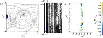


 Open access