


1. Introduction
Cavitation in liquid flows occurs in low-pressure regions close to vapour pressure, and regions most likely to cavitate are those around the lifting surfaces, blade passages of propulsors, etc. These regions are characterised by turbulent shear flows with a complicated web of vortical structures of varied strength and orientation. The first occurrence of cavitation, referred to as cavitation inception, is expected to occur in the cores of stronger vortical structures, characterised by higher circulation, observed in such flows as discussed by Arndt (Reference Arndt2002). For example, in plane shear flows, these vortices would be the stronger, spanwise-oriented ‘primary’ vortices. However, several studies have observed that incipient cavitation occurs in streamwise-oriented, weaker ‘secondary’ vortices in shear flows (Katz & O’hern Reference Katz and O’hern1986; O’hern Reference O’hern1990), wakes (Belahadji, Franc & Michel Reference Belahadji, Franc and Michel1995) and jets (Ran & Katz Reference Ran and Katz1994). Recently, Agarwal et al. (Reference Agarwal, Ram, Lu and Katz2023) examined a turbulent backward-facing step with experimental measurements of three-dimensional velocity fields and inferred pressure fields, using constrained cost minimisation (Agarwal et al. Reference Agarwal, Ram, Wang, Lu and Katz2021) and omni-directional integration (Wang, Zhang & Katz Reference Wang, Zhang and Katz2019). They observed good agreement between inferred low-pressure regions from particle tracking velocimetry (PTV) measurements and the observed cavitation inception locations. They also demonstrated that the weaker vortices present in the flow (quasi-streamwise vortices in their nomenclature) were the corresponding vortical structures that first cavitated in the flow.
Estimating the location and conditions during which cavitation inception occurs is essential to mitigating the adverse effects of cavitation. Although the above studies focused on turbulent shear flows, several previous studies have examined vortex interaction leading to inception in flows with relatively few vortical structures, in the context of cavitation inception in propulsors. Chesnakas & Jessup (Reference Chesnakas and Jessup2003) studied interacting vortices in a shrouded rotor, and observed cavitation inception occurring in relatively weak tip-leakage vortices in the presence of stronger trailing-edge vortices. Experiments by Chang & Ceccio (Reference Chang and Ceccio2011) and Chang et al. (Reference Chang, Choi, Yakushiji and Ceccio2012) examined a simplified system of two counter-rotating vortices produced by a pair of hydrofoils at various attack angles as a simplified laboratory representation of vortex interactions observed in propulsors. The two vortices undergo the long-wavelength Crow instability which leads to strong stretching and pressure drop in the core of the weaker vortex. These studies measured the flow field in the upstream regions before substantial instability occurred. Downstream measurements were performed with high-speed video and hydrophones as the particle imaging velocimetry (PIV) systems of the time did not allow high-speed three-component velocity measurements over a volume. Due to a lack of availability of velocity fields, they were unable to relate observed inception events in secondary vortices to rapid pressure drop. However, Chang & Ceccio (Reference Chang and Ceccio2011) were able to relate the acoustic emissions of inception events to the nuclei population of the water. They showed that smaller nuclei tended to create a ‘pop’ sound (a sharp, broadband acoustic peak) during inception due to their rapid expansion and collapse. In contrast, they found that larger nuclei tended to create a ‘chirp’ sound (with a steady frequency sustained for multiple oscillations). Choi & Ceccio (Reference Choi and Ceccio2007) examined similar acoustic emission phenomena for a single vortex cavitating in the pressure reduction of a venturi configuration. Brandao et al. (Reference Brandao, Madabhushi, Bhatt and Mahesh2020) studied the same pair of counter-rotating vortices leading to cavitation inception as Chang et al. (Reference Chang, Choi, Yakushiji and Ceccio2012) with a computational approach, and found a significant pressure drop in the secondary vortex.
The interaction of a counter-rotating vortex pair undergoing the Crow instability provides a canonical flow through which the vortex inception process may be examined. The interaction of a pair of unequal strength counter-rotating vortices and the resulting flow field was studied in detail by Knister et al. (Reference Knister, Ganesh and Ceccio2026) using a variety of visualisation methods, including volumetric PTV. Volumetric PTV was used to examine the evolution of the vortex properties as they interact, including the local circulation, core size, eccentricity and velocity along the vortex axis. Particular attention was paid to the rate of vortex stretching for the secondary (weaker) vortex as it undergoes strong deformation in the strain field of the primary (stronger) vortex.
The present study reports the relationship between observed cavitation events, underlying pressure fields and nuclei distribution for the configurations discussed in Knister et al. (Reference Knister, Ganesh and Ceccio2026). As in the flow observed by Chang et al. (Reference Chang, Choi, Yakushiji and Ceccio2012), the stretched secondary vortices were observed to be the location of cavitation inception. As before, the weaker vortex experiences substantial stretching as it undergoes the long-wavelength Crow instability. Here, volumetric PTV is used to relate the vortical flow field in and around the stretched secondary vortex to the local pressure reductions in its core. Due to experimental limitations in how rapidly Knister et al. (Reference Knister, Ganesh and Ceccio2026) could track the particles in the cores of the vortices in the downstream region, they used a Reynolds number scaling approach. While the upstream and midstream regions of the flow could be measured over a decade of Reynolds number, the particles in the vortex cores could not be tracked in the downstream region at higher Reynolds number. Accordingly, they used the Reynolds number scaling of the upstream region to infer pressure drops in the cores of the vortices in the downstream region. The inferred distribution of minimum core pressures, in combination with measurements of nuclei in the flow, are used to estimate the inception event rate in the secondary vortices. These estimates are then compared with the acoustically observed inception rates. Finally, the acoustic emissions of the incipient cavitation events themselves are related to the underlying nuclei content of the water as well as the dynamics of the incipient secondary vortices.
2. Experimental set-up and methods
The flow facility, test models and flow visualisation methods were described in detail by Knister et al. (Reference Knister, Ganesh and Ceccio2026). In summary, pairs of cambered NACA66 hydrofoils with root chord of 167 mm were used to generate the pair of counter-rotating line vortices. One pair had matching rectangular planforms with foil tip thickness, $d_s$
, of 15 mm. The other pair had a tapered hydrofoil to generate the secondary vortex, tapering down to a tip thickness of 6.25 mm. These vortices undergo the Crow instability within several chord lengths downstream of the hydrofoils. Figure 1 shows a schematic diagram of the set-up. Volumetric velocimetry was used to measure the non-cavitating vortex properties at several locations downstream of the hydrofoils generating the vortices, with the details of the system described therein. Shake-the-box (STB) PTV (Schanz, Gesemann & Schröder Reference Schanz, Gesemann and Schröder2016; Schröder & Schanz Reference Schröder and Schanz2023) measurements were employed in combination with vortex-in-cell (STB-VIC#) (Jeon, Müller & Michaelis Reference Jeon, Müller and Michaelis2022) for calculating Eulerian field data from Lagrangian particle tracks. The typical spatial resolution of the upstream measurement region was 0.45 mm and the typical spatial resolution of the midstream and downstream regions was 0.35 mm.
$d_s$
, of 15 mm. The other pair had a tapered hydrofoil to generate the secondary vortex, tapering down to a tip thickness of 6.25 mm. These vortices undergo the Crow instability within several chord lengths downstream of the hydrofoils. Figure 1 shows a schematic diagram of the set-up. Volumetric velocimetry was used to measure the non-cavitating vortex properties at several locations downstream of the hydrofoils generating the vortices, with the details of the system described therein. Shake-the-box (STB) PTV (Schanz, Gesemann & Schröder Reference Schanz, Gesemann and Schröder2016; Schröder & Schanz Reference Schröder and Schanz2023) measurements were employed in combination with vortex-in-cell (STB-VIC#) (Jeon, Müller & Michaelis Reference Jeon, Müller and Michaelis2022) for calculating Eulerian field data from Lagrangian particle tracks. The typical spatial resolution of the upstream measurement region was 0.45 mm and the typical spatial resolution of the midstream and downstream regions was 0.35 mm.
(a) A side view of the water channel with primary hydrofoil on the top and a secondary hydrofoil (non-matching) on the bottom of the water tunnel. The section in the middle represents the view through the side window. Downstream of the hydrofoils, high-speed video is taken in the regions outlined with blue boxes and used for visualisation of developed cavitation. The volumetric velocimetry is done at three streamwise locations. The laser comes from below and is shown in green. (b) The layout of the water channel as set up for volumetric velocimetry measurements and viewed from above. The brass hydrofoils are in orange on the right. The green regions downstream of the foils are the locations of the illuminated volumes for velocimetry. The light-purple structures outside the test section are water-filled boxes to allow the cameras (with Scheimpflug adapters) to interrogate the flow from non-orthogonal views. (c) A cartoon of the development of the vortex instability studied here. An upstream measurement (0.7c, where c is foil chord) is taken for the ‘initial conditions’ of the instability. A midstream measurement is taken in the linear regime of the instability (1.2c), and a measurement is taken in the nonlinear regime (1.7c downstream).

2.1. Volumetric velocimetry reference pressure
The STB-VIC# approach was used to estimate the pressure field (with a zero average) with the same temporal and spatial resolution of the velocity field measurements. To estimate the absolute pressure in the flow field, it is necessary to supply a boundary value. Using a larger measurement volume with negligible gradients at the boundary can ensure accurate estimates of pressure within the volume. This was achieved by placing a pressure probe in a region that was within the velocimetry measurement domain but far from where the vortices were to find an absolute pressure that could function as a boundary condition for the STB-VIC# fields. The pressure probe used was a modified Pitot tube with epoxy in its centre such that only the holes around the diameter of the probe were exposed to the flow, thus giving the static pressure at that point. It was connected to an Omega PX419 static pressure transducer with 0.08 % accuracy over a range of 0–200 kPa absolute.
There is a tradeoff between spatial resolution and the thickness of the measurement domain when using optical velocimetry techniques. All particles in the illuminated volume are projected onto the planes of the camera sensors. A thicker volume therefore leads to a higher density of particles in the camera sensor, usually measured in particles per pixel or p.p.p. A higher density of seeding particles in a flow also leads to a higher p.p.p. The limits of a PTV algorithm’s ability track particles is usually found as a function of p.p.p. At high p.p.p., there is then a tradeoff between the density of tracked particles (indirectly the spatial resolution) and the thickness of the illuminated volume. As a relatively thick volume was necessary to measure across the weaker vortex while it was oriented nearly vertically, the spatial resolution was then limited. Further, despite the low speeds used for the downstream study, there is still some level of ejection of particles from the core of the secondary vortex, further hindering high spatial resolution in its core. This limited spatial resolution evidently has some effect, as discussed in § 4.2.
A sketch of the cross-section of the CSM used in this study shows the region of minimum pressure in the annulus of the device.

2.2. Acoustic measurements
Acoustic emissions generated by cavitation bubbles were recorded using a hydrophone that allowed distinguishing between the varied acoustics produced by the varied cavitation bubbles. A Bruel and Kjaer Type 8103 hydrophone was placed on the tunnel top window in a water-filled pocket. The hydrophone was held by a piece of foam to reduce reflections. A Type 2635 Bruel and Kjaer charge amplifier fed the hydrophone signal into a National Instruments 6361 DAQ, which sampled the signal at 500 kHz. The data were filtered digitally in Matlab after acquisition and this processing is detailed in the results section.
2.3. Nuclei measurements
While zero or negative pressures in the liquid are necessary for cavitation inception, a cavitation nucleus is needed to initiate inception, given the magnitude of tensions occurring in the flows studied here (i.e. these flows undergo heterogeneous nucleation) (Brennen Reference Brennen2014). It is therefore necessary to measure the concentration and critical pressure of the free-stream nuclei population when considering the underlying processes responsible for vortex cavitation inception. Various methods, such as interferometric Mie imaging and long-range microscopic shadowgraphy, have been developed for measuring small bubbles that often serve as nuclei (see a discussion in Russell et al. (Reference Russell, Barbaca, Venning, Pearce and Brandner2020)). Such optical methods, however, are less effective for small nuclei such as those in natural nuclei populations that were present during the present experiments. For the range of nuclei size distributions (O(10 μm)) that are relevant here, a cavitation susceptibility meter (CSM) is more suitable. Originally developed by Oldenziel (Reference Oldenziel1982), the CSM flows the channel water through a venturi such that the pressure drops to negative absolute pressures (tensions). A representative diagram is shown in figure 2. As the liquid runs through the tension, the nuclei incept and make a sharp acoustic emission which is detected by a small piezoelectric element. By varying the flow rate, the tension in the throat of the venturi can be varied and measured indirectly by measuring the flow rate and the static pressure upstream. The flow in the CSM throat is swept through a range of tensions, and at each tension, the number of inception events detected by the piezoelectric element is recorded. As the tension is known and the flow rate and time of acquisition are known, the number of nuclei at that critical tension in a given fluid volume is determined. For a given critical tension or pressure, $P_{\textit{critical}}$
, a corresponding critical radius,
$P_{\textit{critical}}$
, a corresponding critical radius, $r_{\textit{critical}}$
, can be found by treating nuclei as spheres of contaminant gas following
$r_{\textit{critical}}$
, can be found by treating nuclei as spheres of contaminant gas following
 \begin{equation} P_{\textit{critical}} = P_{vap} - \frac {4S}{3r_{\textit{critical}}}, \end{equation}
where S is the surface tension. This is known as the Blake critical radius and this relation can be used to determine the size of nuclei that incept at a given critical pressure. However, it is important to note that the nuclei may not be clean gas bubbles but may be the result of any inclusion in the liquid that has a gas pocket (e.g. a Harvey nucleus). These do not appear to have affected the nuclei population significantly after deaeration; the addition of PIV particles of various but known sizes did not affect the measured nuclei distribution after deaeration of the water, indicating that the PIV particles did not function as Harvey nuclei. The CSM employed in the present study is described by Gindroz & Briançon-Marjollet (Reference Gindroz and Briançon-Marjollet1992). The typical duration of the tension that nuclei experience is around 1/20 of the low pressure in the vortices in the present study. As such, there is a possibility of some transient growth in nuclei in the vortices but before inception that would not be captured by the CSM. However, estimating the typical pressure experienced by the nuclei in the vortex cores upstream of the typical inception region showed that the stabilising effect of surface tension did not allow the growth of nuclei in the vortex cores to affect the eventual inception rates.
To ensure that the water in the channel during the CSM measurement has the same nuclei distribution as during cavitation measurements, it is best to run the tunnel at full speed and the lowest pressure used in the cavitation study to allow the nuclei distribution to equilibrate. However, running the water through the channel for a cavitation measurement has the unfortunate tendency to shift the nuclei distribution up (i.e. larger nuclei in higher concentrations) as nuclei can be drawn out of solution as the water experiences the low pressures in the test section. Given the lengthy duration necessary to conduct a complete CSM measurement, shifts in nuclei concentration during the CSM measurement itself are also possible. Figure 3(a) shows the results of several runs of the CSM used in this study to characterise the water. These runs were carried out over two days with the water tunnel sealed and running throughout this time at a minimal speed to circulate the water. While the amount of air in the tunnel should not have changed in this time, the nuclei distribution measured did change. Note that not only does the typical concentration of the nuclei vary by nearly one order of magnitude, but the slope of the nuclei distribution changes substantially as well.
(a) Nuclei distributions measured with the CSM. Data were collected with the CSM over two days with the same tunnel water, sealed in to prevent addition or loss of dissolved gas. Despite the quantity of dissolved gas being fixed, the different runs yield variable nuclei populations. The differences between various runs can be as much as nearly an order of magnitude, and the slope of the nuclei distribution curves can vary substantially as well. The free-stream dissolved oxygen content was 13 %. (b) To demonstrate the shift in nuclei concentration over time, the tunnel conditions were set to produce developed hydrofoil partial cavitation. Then, with the tunnel circulating at low speed, the concentration at a fixed critical pressure corresponding to 2.5 μm was measured repeatedly from almost immediately after and up to the next morning. The free-stream dissolved oxygen content was 13 %.

As noted above and shown by the data in figure 3(a), the nuclei distribution of a particular filling of the channel is not necessarily a fixed quantity even if no outside air is ingested or dissolved air is drawn out via deaeration. The nuclei distribution should be regarded as a dynamic equilibrium between the dissolved gases and the nuclei, and the balance of this equilibrium can shift over time, depending especially on the pressure applied to the water. Figure 3(b) shows the shift in concentration of nuclei with a Blake’s radius of 2.5 μm over time. These measurements were taken immediately after first running the channel with developed cavitation over a hydrofoil for 10 minutes. Following that cavitation, the drift of nuclei concentration over time was recorded. Given the length of time required to measure a full nuclei distribution curve, only the concentration at a single critical tension (equivalent to a Blake’s radius of 2.5 μm) was measured. There is a noticeable drift in the first few minutes, followed by a slower drift. As such, the largest uncertainty in relating the nuclei measurement to the eventual cavitation inception measurements derives from the shift in the nuclei distribution over time. To better account for the effect of drift of nuclei concentration, before inception measurements, the channel was run at the same speed as the inception measurements and comparable pressures for approximately 10 minutes. After this, an initial CSM measurement was taken and following the inception measurements, a final CSM measurement was taken. Nevertheless, the CSM measurement would noticeably change during the duration of the measurement as the nuclei shifted yet again (as suggested by figure 3 b), again by a factor of as much as 2–3. Mitigating these shifts was done by first allowing the tunnel to cycle at a low speed for approximately 10 minutes before beginning the CSM measurement. In all cases in this work, the initial and final CSM measurements were averaged, and as a conservative estimate, the CSM measurements are assumed to be within a factor of 4 of the actual nuclei distribution. Beyond the uncertainties discussed above, bias errors in the CSM measurements must be accounted for. Yakushiji (Reference Yakushiji2009) made a thorough study of potential bias errors of the CSM used here using a combination of numerical models and experiments, and the arguments there are reiterated here for completeness as that work may not be widely available. First, Yakushiji (Reference Yakushiji2009) examined the velocity difference between the sampling line feeding the CSM and the cavitation channel. The velocity difference indicates a corresponding pressure difference and radial slip velocity of the nuclei at the inlet that could lead to a bias error. For a typical range of flow rates and nuclei sizes in the CSM, Yakushiji (Reference Yakushiji2009) found this possible bias error in nuclei density would be less than 10 %. Second, Yakushiji (Reference Yakushiji2009) evaluated the potential bias due to the static pressure difference between the test section and the CSM by numerically solving the Rayleigh–Plesset equation, which was found to cause less than a 5 % reduction in assumed tension in the CSM. Third, Yakushiji (Reference Yakushiji2009) showed that at the highest nuclei density possible for this CSM (−0.1 nuclei per cubic cm), the time between acoustic pulses from inception events may be less than the dead time of the piezoelectric sensor, leading to an undercounting bias. However, with a large negative tension, a single inception event could generate a long-duration acoustic signal instead of a short pulse. This would cause an overcounting bias as a single inception nucleus would be counted as multiple inception events. The effects of under- and overcounting were then evaluated by comparing the acoustic count and a count from high-speed video of the CSM throat. The under-/overcounting bias was found to primarily be a function of the cavitation number at the CSM throat. The cavitation number of the CSM was calculated as
 \begin{equation} \sigma _{\textit{CSM}} = (P_{\textit{up}}-P_{vap})/\left(\frac {\rho }{2} \frac {Q_{\textit{CSM}}^2}{S_{\textit{CSM}}^2}\right)\!, \end{equation}
with $P_{\textit{up}}$
the upstream static pressure (i.e. the tunnel static pressure),
$P_{\textit{up}}$
the upstream static pressure (i.e. the tunnel static pressure), $Q_{\textit{CSM}}$
the flow rate in the CSM throat and
$Q_{\textit{CSM}}$
the flow rate in the CSM throat and $S_{\textit{CSM}}$
the cross-sectional area of the CSM throat. Yakushiji (Reference Yakushiji2009) found an undercounting of nuclei of approximately 90 % occurring at
$S_{\textit{CSM}}$
the cross-sectional area of the CSM throat. Yakushiji (Reference Yakushiji2009) found an undercounting of nuclei of approximately 90 % occurring at $\sigma _{\textit{CSM}}=1$
and a 50 % overcounting occurring at
$\sigma _{\textit{CSM}}=1$
and a 50 % overcounting occurring at $\sigma _{\textit{CSM}}=0.8$
. While these factors appear large, Yakushiji (Reference Yakushiji2009) argues that the largest bias error (under-/overcounting) is minimised around the size of nuclei of greatest interest here (
$\sigma _{\textit{CSM}}=0.8$
. While these factors appear large, Yakushiji (Reference Yakushiji2009) argues that the largest bias error (under-/overcounting) is minimised around the size of nuclei of greatest interest here ( $\sim$
5 to 10 μm). Additionally, by variation of dissolved gas content, the nuclei distributions can be shifted by much larger values than the bias errors discussed, and the primary goal of the nuclei measurements is not necessarily a ‘true’ nuclei density, but a consistent measurement. Beyond the thorough work of Yakushiji (Reference Yakushiji2009) on the CSM used in this work, Khoo et al. (Reference Khoo, Venning, Pearce and Brandner2020) discusses the dramatic variability of nuclei measurements typical of cavitation measurements, even in facilities with more elaborate deaeration and nuclei control systems than that used here (such as the Cavitation Research Laboratory Tunnel at the Australian Maritime College).
$\sim$
5 to 10 μm). Additionally, by variation of dissolved gas content, the nuclei distributions can be shifted by much larger values than the bias errors discussed, and the primary goal of the nuclei measurements is not necessarily a ‘true’ nuclei density, but a consistent measurement. Beyond the thorough work of Yakushiji (Reference Yakushiji2009) on the CSM used in this work, Khoo et al. (Reference Khoo, Venning, Pearce and Brandner2020) discusses the dramatic variability of nuclei measurements typical of cavitation measurements, even in facilities with more elaborate deaeration and nuclei control systems than that used here (such as the Cavitation Research Laboratory Tunnel at the Australian Maritime College).
The free-stream nuclei concentration is related to the dissolved gas content of the free-stream water. The dissolved oxygen (DO) content was measured using a Thermo Scientific Orion 083005MD DO probe with a Thermo Scientific Orion Star A113 meter having a combined uncertainty of 2 % in DO concentration at atmospheric pressure. The DO content is used as a proxy for total dissolved gas content. Setting an arbitrary distribution of nuclei is not possible, but the power-law distribution of natural nuclei can be shifted and estimated using the DO content of the water. The relationship between the DO and the total dissolved gas content is discussed by Yu & Ceccio (Reference Yu and Ceccio1997).
2.4. Test conditions
As described in Knister et al. (Reference Knister, Ganesh and Ceccio2026), pairs of matching and non-matching hydrofoils were examined. The non-matched hydrofoils were examined with the secondary attack angle, $\alpha _{s}$
, at 0°, −2° and −4° (i.e. N.0, N.2 and N.4 conditions), and the matched foils had one set at −4° (M.4). As the secondary foil is set to negative angles of attack (necessary to produce appropriate circulation ratios in the length of the test section), N.4 and M.4 produce the weakest secondary vortices while N.0 produces the strongest. In all cases, the primary hydrofoil was fixed at 6° angle of attack,
$\alpha _{s}$
, at 0°, −2° and −4° (i.e. N.0, N.2 and N.4 conditions), and the matched foils had one set at −4° (M.4). As the secondary foil is set to negative angles of attack (necessary to produce appropriate circulation ratios in the length of the test section), N.4 and M.4 produce the weakest secondary vortices while N.0 produces the strongest. In all cases, the primary hydrofoil was fixed at 6° angle of attack, $\alpha _{p}$
. Table 1 shows all cases studied with velocimetry. The chord-based Reynolds number was
$\alpha _{p}$
. Table 1 shows all cases studied with velocimetry. The chord-based Reynolds number was
 \begin{equation} \textit{Re}_{c} = \frac {U_{0}c}{\nu }, \end{equation}
where $U_{0}$
is the free-stream flow speed,
$U_{0}$
is the free-stream flow speed, $\nu$
is the water kinematic viscosity and c is the hydrofoil base chord length. The inception experiments were conducted with
$\nu$
is the water kinematic viscosity and c is the hydrofoil base chord length. The inception experiments were conducted with $U_{0}$
= 10 m s−1, making
$U_{0}$
= 10 m s−1, making $\textit{Re} = 1.67 \times 10^6$
. The cavitation number,
$\textit{Re} = 1.67 \times 10^6$
. The cavitation number, $\sigma$
, is defined as
$\sigma$
, is defined as
 \begin{equation} \sigma _{c} = \frac {P_{0}-P_{vap}}{\frac {1}{2} \rho U_{0}^{2}}, \end{equation}
where $P_{0}$
is the free-stream pressure,
$P_{0}$
is the free-stream pressure, $P_{vap}$
is the vapour pressure of the water and
$P_{vap}$
is the vapour pressure of the water and $\rho$
is the water density. The uncertainty in the Reynolds number is 0.09 %, and that in the cavitation number is 0.01 %. The DO content was maintained at a ‘low’ concentration of 13 % (
$\rho$
is the water density. The uncertainty in the Reynolds number is 0.09 %, and that in the cavitation number is 0.01 %. The DO content was maintained at a ‘low’ concentration of 13 % ( $\pm$
2 %) and at a ‘high’ concentration of 35 % (
$\pm$
2 %) and at a ‘high’ concentration of 35 % ( $\pm$
2 %). The water temperature varied in a range between 24.0 and 26.1
$\pm$
2 %). The water temperature varied in a range between 24.0 and 26.1 $^\circ$
C.
$^\circ$
C.
The conditions for volumetric velocimetry measurement at the three measurement locations (scaled by foil chord, c). Note that at each streamwise location, three separate volumes had to be set up to adequately measure the vortices as they shifted positions between different cases, but the differences in extent of those different volumes are minimal. In all cases, the primary hydrofoil was fixed at $\alpha _{\!P}$
= 6°.
$\alpha _{\!P}$
= 6°.

Figure 1(a) shows a schematic of the configuration with the primary and secondary hydrofoils on the top and bottom window, respectively. Downstream of the hydrofoils, high-speed video is taken in the regions outlined with blue boxes and used for visualisation of developed cavitation (to be discussed later). The volumetric velocimetry is done at three streamwise locations shown in green. Four secondary hydrofoil arrangements generating counter-rotating vortices were examined in detail with the primary hydrofoil fixed at +6° angle of attack. The arrangements are denoted by ‘M’ or ‘N’ for a matching or non-matching (tapered) secondary hydrofoil planform set-up. A digit represents the negative angle of attack of the secondary hydrofoil, and the four conditions are therefore denoted as N.0, N.2, N.4 and M.4. Two of these, M.4 and N.4, which have the secondary at −4° angle of attack, were examined over a range of flow speeds to examine the effect of chord-based Reynolds number ( $\textit{Re}_{c}$
) on the formation of the vortices, where
$\textit{Re}_{c}$
) on the formation of the vortices, where $\nu$
is the kinematic viscosity of water at room temperature. The cavitation number is defined using (2.4), where
$\nu$
is the kinematic viscosity of water at room temperature. The cavitation number is defined using (2.4), where $P_{0}$
is the test-section inlet pressure,
$P_{0}$
is the test-section inlet pressure, $P_{v}$
is the vapour pressure of water and
$P_{v}$
is the vapour pressure of water and $\rho$
is the water density.
$\rho$
is the water density.
A cartoon of these regions is shown in figure 1(c) and the conditions of measurements in these regions are shown in table 1.
3. Observations of cavitation inception in the secondary vortices
Knister et al. (Reference Knister, Ganesh and Ceccio2026) used developed cavitation to visualise the vortical flow interaction. Figure 4 (also shown in Knister et al. Reference Knister, Ganesh and Ceccio2026) shows an instantaneous realisation of the vortical flow with developed cavitation for all cases at $\textit{Re}= 1.67 \times 10^6$
and
$\textit{Re}= 1.67 \times 10^6$
and $\sigma$
= 0.94. While the secondary vortex is initially above the primary vortex, it orbits the stronger vortex and moves below it. Both vortices convect downward due to their respective actions on each other, but the primary vortex does not convect downward as much as the secondary in this case due to the secondary vortex being weaker relative to the primary. While the vortices are both initially close to linear in shape, the secondary vortex develops a sinuous instability and wraps around the primary vortex. In this process, the secondary vortex begins to break apart to form vortex rings, although in case N.4 this breakup into rings is slower and not often visible within the test section. The primary sometimes also breaks down as a vortex. The secondary vortex has a lower circulation and a smaller core diameter than the primary. Knister et al. (Reference Knister, Ganesh and Ceccio2026) discuss the kinematics of interaction of the vortices for the different conditions in detail.
$\sigma$
= 0.94. While the secondary vortex is initially above the primary vortex, it orbits the stronger vortex and moves below it. Both vortices convect downward due to their respective actions on each other, but the primary vortex does not convect downward as much as the secondary in this case due to the secondary vortex being weaker relative to the primary. While the vortices are both initially close to linear in shape, the secondary vortex develops a sinuous instability and wraps around the primary vortex. In this process, the secondary vortex begins to break apart to form vortex rings, although in case N.4 this breakup into rings is slower and not often visible within the test section. The primary sometimes also breaks down as a vortex. The secondary vortex has a lower circulation and a smaller core diameter than the primary. Knister et al. (Reference Knister, Ganesh and Ceccio2026) discuss the kinematics of interaction of the vortices for the different conditions in detail.
Developed cavitation in the vortices generated by the hydrofoils aids in the visualisation of the instability. Properties of the secondary vortex (blue) in all cases change resulting in different instability development and interaction flow features. The images shown here are a side view of the cavitation. The right-hand column of images spans approximately (0.2–1.2)c downstream of the foils and the left-hand column of images spans approximately (1.3–2.3)c downstream.

At higher free-stream pressures, the vortex cores will not be filled with vapour, resulting in the absence of developed cavitation shown in figure 4. However, cavitation can occur when the local pressure is low enough to cause a nucleation site to grow, resulting in inception. Figure 5 shows the time series of cavitation inception occurring in the region of nonlinear interaction for case M.4 at $\textit{Re} = 1.67 \times 10^6$
and
$\textit{Re} = 1.67 \times 10^6$
and $\sigma$
= 1.34. As observed in previous studies, incipient cavitation occurred in the cores of the stretched secondary vortices, not the stronger primary vortex. For condition M.4 shown in figure 5, cavitation initiates in the leg and persists past the downstream extent of the high-speed camera, with a lifetime longer than 8 ms. Upon initiation, cavitation propagates from the vertically oriented leg region to the horizontally oriented peak region in the vortex. Often, for events where cavitation initiates in the vortex legs and persists for a considerable length of time, the cavitation propagated into the peaks. Sometimes, as the peak begins to cavitate, the leg where cavitation is initiated will cease to cavitate, as shown here. In other events, after initiating in the leg, the cavitation will continue in the leg while propagating through the peak.
$\sigma$
= 1.34. As observed in previous studies, incipient cavitation occurred in the cores of the stretched secondary vortices, not the stronger primary vortex. For condition M.4 shown in figure 5, cavitation initiates in the leg and persists past the downstream extent of the high-speed camera, with a lifetime longer than 8 ms. Upon initiation, cavitation propagates from the vertically oriented leg region to the horizontally oriented peak region in the vortex. Often, for events where cavitation initiates in the vortex legs and persists for a considerable length of time, the cavitation propagated into the peaks. Sometimes, as the peak begins to cavitate, the leg where cavitation is initiated will cease to cavitate, as shown here. In other events, after initiating in the leg, the cavitation will continue in the leg while propagating through the peak.
The observed inception location and its propagation depended on the configuration studied. For example, for the N.4 inception instance in figure 6, inception occurred in the leg; however, it collapsed soon after with a lifetime of approximately 5 ms, before it could propagate out of the field of view. This inception event takes an approximately vertical orientation of the leg, but it does not extend the full length of the secondary vortex leg at that location. Supplementary movies available at https://doi.org/10.1017/jfm.2026.11441 show the processes for the cases discussed above. The location of inception and the subsequent propagation of cavitation provide qualitative information about the nature of the pressure fields during vortex interaction, which will be discussed next.
Cavitation inception in case M.4 at Re = $1.67 \times 10^6$
and
$1.67 \times 10^6$
and $\sigma$
= 1.34 shows that inception begins in the leg of the secondary vortex in this event. The inception then propagates down to the trough of the secondary vortex and not up to the peak. Cavitation persists until this segment of the vortex propagates out of the field of view of the camera, for at least 8 ms. Supplementary movies show the occurrence of inception processes for the cases shown in table 1. The colour is inverted from the developed cavitation visualisations. The width of each image here is approximately 0.45c and they are centred around 2c downstream of the foils.
$\sigma$
= 1.34 shows that inception begins in the leg of the secondary vortex in this event. The inception then propagates down to the trough of the secondary vortex and not up to the peak. Cavitation persists until this segment of the vortex propagates out of the field of view of the camera, for at least 8 ms. Supplementary movies show the occurrence of inception processes for the cases shown in table 1. The colour is inverted from the developed cavitation visualisations. The width of each image here is approximately 0.45c and they are centred around 2c downstream of the foils.

Cavitation inception in case N.4 at Re = $1.67 \times 10^6$
and
$1.67 \times 10^6$
and $\sigma$
= 2.14 shows that inception begins in the leg of the secondary vortex in this event. The inception then propagates somewhat down towards the trough of the secondary vortex before collapsing after less than 5 ms, in contrast to the persistence of cavitation in figure 5. Supplementary movies show the occurrence of inception processes for the cases shown in table 1. The colour is inverted from the developed cavitation visualisations. The width of these images is approximately 0.5c and they are centred around 1.8c downstream of the foils.
$\sigma$
= 2.14 shows that inception begins in the leg of the secondary vortex in this event. The inception then propagates somewhat down towards the trough of the secondary vortex before collapsing after less than 5 ms, in contrast to the persistence of cavitation in figure 5. Supplementary movies show the occurrence of inception processes for the cases shown in table 1. The colour is inverted from the developed cavitation visualisations. The width of these images is approximately 0.5c and they are centred around 1.8c downstream of the foils.

4. Estimation of the time-varying pressure in the secondary vortex cores
Knister et al. (Reference Knister, Ganesh and Ceccio2026) discuss the kinematics of the vortex interaction to reveal the time-varying circulation and core sizes of the stretched secondary vortices, including the classification of the secondary topology as legs, troughs and peaks. The measurements from that study are used to infer the core pressure variation of the secondary vortices here. Knister et al. (Reference Knister, Ganesh and Ceccio2026) showed that axial straining and jetting had a minimal effect on the secondary vortex flow, with the most prominent effect being a reduction in the viscous core size. Figure 7 shows the typical core size of the secondary vortex for the various cases in the upstream, midstream and downstream locations. While the difference between upstream and midstream radii is relatively small, the radius is significantly reduced in the downstream location. This results in a correspondingly significant drop in pressure in the secondary vortex core.
Comparison of secondary vortex radius for different configurations across different locations. (a) The variation of vortex radius at different locations for the configurations considered. (b) The vortex core radius measured in the legs, troughs and overall. (c) The change in vortex circulation measured at different locations for different configurations considered. No appreciable change in circulation is measured; however, the vortex core radius reduces suggesting an increase in peak vorticity.

4.1. Core pressure estimates using volumetric PTV
As described in § 2, volumetric PTV measurements were used to determine the local pressure in the measured domain around the secondary vortex using STB-VIC#. Three independent sets of 15 000 images were taken to calculate the STB-VIC# fields. The velocity data were also used to determine the local vortex circulation, $\varGamma$
, and core size,
$\varGamma$
, and core size, $r_C$
. There is a strong correlation between the computed pressure drop,
$r_C$
. There is a strong correlation between the computed pressure drop, $P_{\textit{drop}}$
, in the secondary vortex and its vortex properties. For an isolated line vortex,
$P_{\textit{drop}}$
, in the secondary vortex and its vortex properties. For an isolated line vortex,
 \begin{equation} P_{\textit{drop}} \sim - \frac {\varGamma ^2}{r_C^2}. \end{equation}
Applying this relationship to the present study, a correlation coefficient of approximately −0.85 to −0.9 between $P_{\textit{drop}}$
and
$P_{\textit{drop}}$
and $\varGamma ^2/r_C^2$
was observed for all four cases. The secondary vortex radius, scaled by foil tip width, d, is shown in figure 7(a).
$\varGamma ^2/r_C^2$
was observed for all four cases. The secondary vortex radius, scaled by foil tip width, d, is shown in figure 7(a).
4.2. Limitations of volumetric PTV and the need for Reynolds scaling
The vortex total circulation is expected to be conserved in this flow. The circulation in the primary vortex is conserved within uncertainty of the measurements. However, there is a noticeable drop in the measured circulation of the secondary vortices between the upstream and the downstream measurements, as shown in figure 7(c). Some diffusion of vorticity can be expected due to finite viscosity as is discussed in Knister et al. (Reference Knister, Ganesh and Ceccio2026). In summary, the limited spatial resolution of the velocimetry of the secondary vortex can result in an underestimation of the strength of vortex circulation and accordingly an underestimation of pressure drop in the secondary vortex.
In addition, temporal resolution of the vortex interactions at the same Re (flow speed) as the cavitation inception study is challenging. For STB to track particles with high accelerations, like those in the secondary vortex cores here, the typical displacement could not be more than 5–7 pixels. At higher Reynolds number, keeping the displacements to this level requires faster acquisition, which is constrained by the maximum frame rate of the camera as well as the reduction in laser power above 10 kHz. Knister et al. (Reference Knister, Ganesh and Ceccio2026) showed that there was little Reynolds number dependence in the initial circulation of the secondary vortex for Reynolds numbers above 0.3 × 10⁶, roughly fixing upstream secondary circulation, $\varGamma _{s,US}$
. The resolution of the low-Reynolds-number flow is much improved compared with those at the highest speeds where the inception study was conducted, as discussed in detail by Knister et al. (Reference Knister, Ganesh and Ceccio2026). Low speeds make the measurement of downstream secondary circulation,
$\varGamma _{s,US}$
. The resolution of the low-Reynolds-number flow is much improved compared with those at the highest speeds where the inception study was conducted, as discussed in detail by Knister et al. (Reference Knister, Ganesh and Ceccio2026). Low speeds make the measurement of downstream secondary circulation, $\varGamma _{s,DS}$
, much more resolved at lower Re compared with Re = 1.67 × 10⁶ (
$\varGamma _{s,DS}$
, much more resolved at lower Re compared with Re = 1.67 × 10⁶ ( $U_0$
= 10 m s−1), the flow condition under which the inception events were examined. This is due to limited spatial resolution in the core region of the stretched secondary vortex, as discussed above. Assuming that the circulation ratio measured in the low Re = 0.5 × 10⁶ case is equivalent to the ratio at high Re, the well-resolved, low-Re pressure data can be scaled to infer the pressure drop at higher Re corresponding to the cavitation experiments. Accordingly, the ratio of the resolved pressure data derived from the Re = 0.5 × 10⁶ (
$U_0$
= 10 m s−1), the flow condition under which the inception events were examined. This is due to limited spatial resolution in the core region of the stretched secondary vortex, as discussed above. Assuming that the circulation ratio measured in the low Re = 0.5 × 10⁶ case is equivalent to the ratio at high Re, the well-resolved, low-Re pressure data can be scaled to infer the pressure drop at higher Re corresponding to the cavitation experiments. Accordingly, the ratio of the resolved pressure data derived from the Re = 0.5 × 10⁶ ( $U_0$
= 3 m s−1) case is scaled using the ratio of the secondary vortex upstream circulation measured for Re = 0.5 × 10⁶ (
$U_0$
= 3 m s−1) case is scaled using the ratio of the secondary vortex upstream circulation measured for Re = 0.5 × 10⁶ ( $U_0$
= 3 m s−1) and Re = 1.67 × 10⁶ (
$U_0$
= 3 m s−1) and Re = 1.67 × 10⁶ ( $U_0$
= 10 m s−1). This is approximately equal to the square of the free-stream velocity ratio
$U_0$
= 10 m s−1). This is approximately equal to the square of the free-stream velocity ratio $(10/3)^2$
.
$(10/3)^2$
.
The core pressure drop, $P_0 - P_{\textit{CV}}$
, is then estimated with the scaled velocimetry data. At present, there is not a generally accepted method of estimating the uncertainty of pressure calculated by VIC# or other data assimilation approaches from PTV particle tracks. Zhou et al. (Reference Zhou, Grauer, Schanz, Godbersen, Schroder, Rockstroh, Jeon and Wieneke2024) and Sciacchitano, Leclaire & Schroder (Reference Sciacchitano, Leclaire and Schroder2025) examined several leading algorithms for data assimilation of Lagrangian particle tracks over multiple synthetic flow configurations, including results for pressure estimation. Besides the effects of the different algorithms, the seeding density had the greatest effect on the eventual results. The seeding density was manipulated in both studies removing random particles. Fewer particles led to less accurate results compared to the ground truth, which is expected as the particles function as the sensors in optical velocimetry measurements. A reduction in the density of tracked particles is then a reduction in spatial resolution, making it more difficult for a data assimilation approach such as VIC# to evaluate quantities such as pressure. Given the lack of an accepted approach for estimating the uncertainty of pressure from data assimilation, we assume that it follows typical behaviour found by the comparison studies of Zhou et al. (Reference Zhou, Grauer, Schanz, Godbersen, Schroder, Rockstroh, Jeon and Wieneke2024) and Sciacchitano et al. (Reference Sciacchitano, Leclaire and Schroder2025). Sciacchitano et al. (Reference Sciacchitano, Leclaire and Schroder2025) explicitly note the accuracy of pressure reconstruction as a function of the seeding density, and the typical error there is used as an a posteriori estimate of the uncertainty of our pressure reconstruction. It should be noted that the uncertainty of pressure from STB-VIC# is in reality a temporally and spatially varying quantity as the random error will depend strongly on the typical particle spacing relative to the local flow structures. However, a typical estimate is sought here. For the case of comparable seeding density (in terms of particles per pixel) to the present study, Sciacchitano et al. (Reference Sciacchitano, Leclaire and Schroder2025) found that pressure reconstructions of large free-stream vortical structures with VIC# accurately determine pressure minima to within 10 % of the ground truth. We accordingly expect comparable accuracy for the data here, though the inter-particle spacing relative to the vortical structure diameter is slightly higher in the secondary vortex measurements discussed in this study.
$P_0 - P_{\textit{CV}}$
, is then estimated with the scaled velocimetry data. At present, there is not a generally accepted method of estimating the uncertainty of pressure calculated by VIC# or other data assimilation approaches from PTV particle tracks. Zhou et al. (Reference Zhou, Grauer, Schanz, Godbersen, Schroder, Rockstroh, Jeon and Wieneke2024) and Sciacchitano, Leclaire & Schroder (Reference Sciacchitano, Leclaire and Schroder2025) examined several leading algorithms for data assimilation of Lagrangian particle tracks over multiple synthetic flow configurations, including results for pressure estimation. Besides the effects of the different algorithms, the seeding density had the greatest effect on the eventual results. The seeding density was manipulated in both studies removing random particles. Fewer particles led to less accurate results compared to the ground truth, which is expected as the particles function as the sensors in optical velocimetry measurements. A reduction in the density of tracked particles is then a reduction in spatial resolution, making it more difficult for a data assimilation approach such as VIC# to evaluate quantities such as pressure. Given the lack of an accepted approach for estimating the uncertainty of pressure from data assimilation, we assume that it follows typical behaviour found by the comparison studies of Zhou et al. (Reference Zhou, Grauer, Schanz, Godbersen, Schroder, Rockstroh, Jeon and Wieneke2024) and Sciacchitano et al. (Reference Sciacchitano, Leclaire and Schroder2025). Sciacchitano et al. (Reference Sciacchitano, Leclaire and Schroder2025) explicitly note the accuracy of pressure reconstruction as a function of the seeding density, and the typical error there is used as an a posteriori estimate of the uncertainty of our pressure reconstruction. It should be noted that the uncertainty of pressure from STB-VIC# is in reality a temporally and spatially varying quantity as the random error will depend strongly on the typical particle spacing relative to the local flow structures. However, a typical estimate is sought here. For the case of comparable seeding density (in terms of particles per pixel) to the present study, Sciacchitano et al. (Reference Sciacchitano, Leclaire and Schroder2025) found that pressure reconstructions of large free-stream vortical structures with VIC# accurately determine pressure minima to within 10 % of the ground truth. We accordingly expect comparable accuracy for the data here, though the inter-particle spacing relative to the vortical structure diameter is slightly higher in the secondary vortex measurements discussed in this study.
Trace of the estimated pressure drop in the secondary vortex over time for case N.2, scaled by the circulation of the primary vortex, $\varGamma$
, and the (upstream) separation distance,
$\varGamma$
, and the (upstream) separation distance, $b_0$
, to give a sense of how the pressure varies over time.
$b_0$
, to give a sense of how the pressure varies over time.

The vortex core pressure coefficient, $C_{\!\textit{PV}}$
, is defined as
$C_{\!\textit{PV}}$
, is defined as
 \begin{equation} C_{\!\textit{PV}} = \frac {P_{\textit{CV}} - P_0}{\frac {1}{2}\rho U_0^2}. \end{equation}
Time series of $-C_{\!\textit{PV}}$
are provided in figure 8 for case N.2 to illustrate how it varies with the vortex interaction over time. Figures 9(a) and 9(b) show histograms of pressure drop in the secondary vortex as a whole and in vortex legs.
$-C_{\!\textit{PV}}$
are provided in figure 8 for case N.2 to illustrate how it varies with the vortex interaction over time. Figures 9(a) and 9(b) show histograms of pressure drop in the secondary vortex as a whole and in vortex legs.
The pressure drop, the reduction in core pressure in the secondary vortex (a) relative to the free-stream pressure far from the vortices, is estimated to be greater in regions identified as the legs (b) of the secondary vortex for all cases shown in different colours.

Note that a large negative value of $C_{\!\textit{PV}}$
implies a large reduction on core pressure compared with the free-stream pressure, and when
$C_{\!\textit{PV}}$
implies a large reduction on core pressure compared with the free-stream pressure, and when $\sigma = -C_{\!\textit{PV}}$
, the local core pressure has reached vapour pressure. If
$\sigma = -C_{\!\textit{PV}}$
, the local core pressure has reached vapour pressure. If $\sigma \lt -C_{\!\textit{PV}}$
, the liquid in the vortex core is in tension. Note that the values of
$\sigma \lt -C_{\!\textit{PV}}$
, the liquid in the vortex core is in tension. Note that the values of $\sigma$
for the cavitation inception observations for cases M.4 (figure 5) and N.4 (figure 6) are
$\sigma$
for the cavitation inception observations for cases M.4 (figure 5) and N.4 (figure 6) are $\sigma$
= 1.34 and 2.14, respectively. The findings show that the core pressures are sufficiently reduced to achieve transient periods of tensions based on the distributions of
$\sigma$
= 1.34 and 2.14, respectively. The findings show that the core pressures are sufficiently reduced to achieve transient periods of tensions based on the distributions of $C_{\!\textit{PV}}$
.
$C_{\!\textit{PV}}$
.
Upon examining figure 9(b), it is observed that the pressure drop is highest in the cores of the legs compared with the other regions of the vortices. The observed trend is attributed to the reduced radii of the secondary vortex in the legs, which is likely due to greater stretching. The estimated minimum vortex pressures will now be used to estimate cavitation inception rates in the following section for the known free-stream distribution of nuclei.
5. Measured and estimated vortex cavitation inception rates
The distribution of minimum core pressures developed in the previous section will be used to estimate the rate of cavitation inception events for a given free-stream pressure (i.e. cavitation number) and nuclei distribution. These inferred inception event rates can then be compared with the directly observed cavitation inception rates.
5.1. Estimating the concentration of nuclei in the secondary vortex core
An estimate of the inception rate can be developed with knowledge of the concentration and size distribution of nuclei in the secondary vortex core and the likelihood that a given nucleus will experience a tension necessary for inception. The distribution of tensions was discussed earlier and will be used later. The relationship between free-stream nuclei concentration and the nuclei concentration in the vortex core will now be discussed. First, we will assume that the nuclei present in the secondary are the only nuclei available to incept. The nuclei available for cavitation are then assumed to be equivalent to the free-stream nuclei distribution multiplied by the volume flux of liquid in the core of the secondary. The flux is found by the velocimetry measurements, multiplying the average axial velocity in the vortices (averaging in time and across a cross-section of the vortices) by the averaged vortex area. Therefore, we are ignoring the possible capture of nuclei by the vortex. Just as the seeding particles are expelled from the vortex due to their higher density than that of the surrounding water, buoyant nuclei bubbles may be captured from the surrounding flow and brought into the secondary cores. Oweis et al. (Reference Oweis, van der Hout, Iyer, Tryggvason and Ceccio2005) examined this situation in detail with a combination of computational modelling and experiments on nuclei generated a small distance from a vortex. Using their approach, the effects of nuclei capture can be estimated, considering nuclei as individual bubbles of non-condensable gas. A one-way coupled model, with the bubble transported by the flow but the flow unaffected by the bubble, was created. The model developed assumes that the bubbles experience small radial accelerations and that the Basset history term, gravitational effects and volume variation effects are small. The remaining pressure gradient forces and drag forces on the bubble were found to capture well the behaviour of the experiments. Assuming a Gaussian vortex, this then leads to an estimate for capture time for a bubble. By setting this capture time to be equal to the time required for the vortex to transit from the foils to the location of most likely inception, $\tau _{\textit{transit}}$
, the capture radius of the vortex can then be estimated by
$\tau _{\textit{transit}}$
, the capture radius of the vortex can then be estimated by
 \begin{equation} r_{\textit{capture}} = \sqrt [^4]{\tau _{\textit{transit}}\frac {2}{9\pi ^2}\frac {r_{\textit{nuclei}}^2{\varGamma }^2}{\nu }}, \end{equation}
where none of the terms are non-dimensionalised and $r_{\textit{nuclei}}$
is the radius of the contaminant gas bubble considered. This radius is estimated by the Blake critical radius introduced above (so,
$r_{\textit{nuclei}}$
is the radius of the contaminant gas bubble considered. This radius is estimated by the Blake critical radius introduced above (so, $r_{\textit{nuclei}} = r_{\textit{critical}}$
over a range of critical tensions). The capture radius is only increased by a factor of 2 for relatively large nuclei around 10 μm in size. Using the Blake critical radius and CSM measurements of the present study, it is found that the prevalence of nuclei of 1 μm radius is approximately 5 orders of magnitude greater than that of nuclei of 10 μm radius. While the apparent increase in capture radius is significant for larger bubbles, the larger bubbles are uncommon, so the overall effect of nuclei capture was found to be negligible when implemented in the model. Second, we will neglect the change in the nuclei critical radius due to the process of gas diffusion while it is resident in the low-pressure vortex core. As nuclei convect in the core of the secondary vortex, they experience reduced pressure, perhaps even tension. In such cases, the water may be locally supersaturated, and dissolved gas will tend to diffuse into the nuclei. With more non-condensable gas inside them, the nuclei will be larger and therefore require less tension to incept. This could shift the nuclei distribution curve. These effects can be estimated by examining the time scale of diffusion relative to the time it takes the flow to travel between the vortex generation at the foils and the most likely point of cavitation inception. Following Brennen (Reference Brennen2014), we estimate the time scale of significant bubble growth via diffusion with
$r_{\textit{nuclei}} = r_{\textit{critical}}$
over a range of critical tensions). The capture radius is only increased by a factor of 2 for relatively large nuclei around 10 μm in size. Using the Blake critical radius and CSM measurements of the present study, it is found that the prevalence of nuclei of 1 μm radius is approximately 5 orders of magnitude greater than that of nuclei of 10 μm radius. While the apparent increase in capture radius is significant for larger bubbles, the larger bubbles are uncommon, so the overall effect of nuclei capture was found to be negligible when implemented in the model. Second, we will neglect the change in the nuclei critical radius due to the process of gas diffusion while it is resident in the low-pressure vortex core. As nuclei convect in the core of the secondary vortex, they experience reduced pressure, perhaps even tension. In such cases, the water may be locally supersaturated, and dissolved gas will tend to diffuse into the nuclei. With more non-condensable gas inside them, the nuclei will be larger and therefore require less tension to incept. This could shift the nuclei distribution curve. These effects can be estimated by examining the time scale of diffusion relative to the time it takes the flow to travel between the vortex generation at the foils and the most likely point of cavitation inception. Following Brennen (Reference Brennen2014), we estimate the time scale of significant bubble growth via diffusion with
 \begin{equation} \tau _{\textit{diffusion}} = \frac {\rho _{\textit{gas}}r_{\textit{bubble}}^2}{D_{\textit{gas}}\Delta \chi }, \end{equation}
where $D_{\textit{gas}}$
is the diffusion coefficient of air in water and
$D_{\textit{gas}}$
is the diffusion coefficient of air in water and $\Delta \chi$
is the concentration differential between the bubble and the free stream. The value of
$\Delta \chi$
is the concentration differential between the bubble and the free stream. The value of $D_{\textit{gas}}$
is generally accepted to be around
$D_{\textit{gas}}$
is generally accepted to be around $2 {\times }10^{-9}\ \rm m^2\,s^{-1}$
(Brennen Reference Brennen2014). Gowing (Reference Gowing1992) examined this coefficient over a decade of Reynolds number in turbulent pipe flow, a situation where diffusion is likely higher than the present vortical flow, and found only a modest increase. Using the higher values reported by Gowing (Reference Gowing1992), overestimating the effect of diffusion, the time scale for diffusion is still substantially greater than the time the nuclei spend travelling in the vortex before inception:
$2 {\times }10^{-9}\ \rm m^2\,s^{-1}$
(Brennen Reference Brennen2014). Gowing (Reference Gowing1992) examined this coefficient over a decade of Reynolds number in turbulent pipe flow, a situation where diffusion is likely higher than the present vortical flow, and found only a modest increase. Using the higher values reported by Gowing (Reference Gowing1992), overestimating the effect of diffusion, the time scale for diffusion is still substantially greater than the time the nuclei spend travelling in the vortex before inception:
 \begin{equation} \frac {\tau _{\textit{diffusion}}}{\tau _{\textit{transit}}} \gg 1. \end{equation}
The effects of gas diffusion on the nuclei population in the vortex core then can be neglected.
5.2. Direct measurement of cavitation inception events in the secondary vortex
High- and low-nuclei-concentration experiments were performed for each hydrofoil configuration for a range of free-stream pressures. As the models needed to be switched between matching and non-matching foil cases, the nuclei distributions were not identical between the matching and non-matching cases, which resulted in two sets of high- and low-nuclei-concentration measurements. These concentrations were approximated by the DO concentration with high being 35 % ( $\pm$
2 %) and low being 13 % (
$\pm$
2 %) and low being 13 % ( $\pm$
2 %) of saturation at atmospheric pressure. The nuclei concentrations were measured by the CSM before and after each inception experiment, so the small differences between the matching and non-matching nuclei concentrations are known and can be accounted for.
$\pm$
2 %) of saturation at atmospheric pressure. The nuclei concentrations were measured by the CSM before and after each inception experiment, so the small differences between the matching and non-matching nuclei concentrations are known and can be accounted for.
To ensure that the effects of nuclei outgassing and drifting are represented in the measurements, the tunnel was allowed to run at full experimental speed and low enough pressure to cause developed cavitation in the vortices before the initial CSM measurements were made. Ideally, this should set the nuclei distribution in the appropriate point of equilibrium such that it does not change due to the cavitation inception measurements. Figures 10(a) and 10(b) show the nuclei concentration measured for the non-matched and matched foil inception experiments.
A combination of high-speed video and acoustic measurements was used to detect inception in the secondary vortex. These two measurements can be synchronised; however, the amount of data generated by a camera is orders of magnitude more than that generated by a hydrophone. The cameras only recorded a portion of the events over the duration of the hydrophone measurements. Hence, the video measurements served primarily to confirm that inception occurs first in the secondary for the vortex configurations considered here. The acoustic data were interpreted by a code that first found peaks in pressure, presumed to correspond to cavitation events. After this, segments of the acoustic signal were examined by spectrogram to look for lengthy (more than 0.1 s) signals preceding the peak. These lengthier signals were found by comparison with camera recordings to result from pseudocavitation in the primary or secondary vortex, and these sequences were discounted as not being true inception events. Pseudocavitation is characterised by non-condensable gas bubbles expanding and contracting in a fashion similar to cavitation bubbles but without any phase change of the water. While pseudocavitation events may oscillate in a similar fashion to the cavitation events studied here, they do so upstream of the typical inception region and accordingly generate longer acoustic signals, so removing lengthy acoustic emission events removes the pseudocavitation events from the inception acoustics. Accumulating all acoustically detected inception events, the resulting event rates are determined for a given foil configuration and free-stream cavitation number.
Nuclei concentration for the several cases are shown. (a) The non-matching cases and (b) the matching case. Changing the secondary hydrofoils between cases necessitated opening the tunnel to outside air and some refilling. For all cases, the low-DO condition corresponds to 13 % (±2 %) of saturation at atmospheric pressure. The high-DO condition corresponds to 35 % (±2 %) of saturation at atmospheric pressure. At each dissolved gas content, the nuclei content was measured with a CSM to give the nuclei concentration shown here.

The CSM measurements of figure 10 are used to estimate the nuclei flux rate through the secondary vortex for all cases, as shown on the left-hand axes and circular symbols. The right-hand axes and triangular symbols give the acoustically measured inception event rate. Note that these are on the same scale, suggesting that the matching of them depends on the relation of the pressure drop in the vortices to the critical pressure of the nuclei. Cases (a) N.0, (b) N.2, (c) N.4 and (d) M.4.

The free-stream nuclei content is used to calculate the nuclei flux in the vortices by
 \begin{equation} Q_{\textit{nuclei}}(p_{\textit{critical}}) = \kappa (p_{\textit{critical}}) u_{s, avg} \pi r_{c,s}^2, \end{equation}
where $Q_{\textit{nuclei}}$
is taken as a function of critical pressure and calculated as the product of
$Q_{\textit{nuclei}}$
is taken as a function of critical pressure and calculated as the product of $\kappa$
, the free-stream nuclei concentration from the CSM (a function of critical pressure),
$\kappa$
, the free-stream nuclei concentration from the CSM (a function of critical pressure), $u_{s,avg}$
, the spatially and temporally averaged axial velocity in the secondary vortex core, and
$u_{s,avg}$
, the spatially and temporally averaged axial velocity in the secondary vortex core, and $r_{c,s}$
, the radius of the secondary vortex core. The secondary vortex core properties are evaluated at the upstream measurement location. The measured cavitation inception rates are plotted in figure 11 along with the nuclei flux rates. Given the rather strong secondary vortex for case N.0, only a small range of free-stream cavitation numbers could be measured for this case and only at low free-stream nuclei concentrations. At lower pressures, the vortices exhibited developed cavitation as opposed to incipient cavitation. With higher dissolved gas concentration, the occurrence of developed cavitation or pseudocavitation in the secondary vortex in the feasible range of pressures was observed, so measurements were not taken at the higher dissolved gas concentration. Several observations can be made from findings reported in figure 11. In comparison to N.0, the event rate for N.2 is shifted left or down, showing the weaker pressure drop in this case. In comparison to N.2, for N.4, the nuclei flux rate and event rate are shifted left or down, showing the lower amount of available nuclei for cavitation due to the smaller radius for N.4 as well as the somewhat weaker pressure drop in N.4 relative to N.2. It should be noted that while the high and low DO contents are nominally the same between the matched and non-matched cases, the nuclei distribution of case M.4 was measured to be different from that of the preceding cases, so direct comparison between M.4 and the other cases is not possible. Still, the observed event rates for M.4 are comparable to those of N.2 and N.4.
$r_{c,s}$
, the radius of the secondary vortex core. The secondary vortex core properties are evaluated at the upstream measurement location. The measured cavitation inception rates are plotted in figure 11 along with the nuclei flux rates. Given the rather strong secondary vortex for case N.0, only a small range of free-stream cavitation numbers could be measured for this case and only at low free-stream nuclei concentrations. At lower pressures, the vortices exhibited developed cavitation as opposed to incipient cavitation. With higher dissolved gas concentration, the occurrence of developed cavitation or pseudocavitation in the secondary vortex in the feasible range of pressures was observed, so measurements were not taken at the higher dissolved gas concentration. Several observations can be made from findings reported in figure 11. In comparison to N.0, the event rate for N.2 is shifted left or down, showing the weaker pressure drop in this case. In comparison to N.2, for N.4, the nuclei flux rate and event rate are shifted left or down, showing the lower amount of available nuclei for cavitation due to the smaller radius for N.4 as well as the somewhat weaker pressure drop in N.4 relative to N.2. It should be noted that while the high and low DO contents are nominally the same between the matched and non-matched cases, the nuclei distribution of case M.4 was measured to be different from that of the preceding cases, so direct comparison between M.4 and the other cases is not possible. Still, the observed event rates for M.4 are comparable to those of N.2 and N.4.
5.3. Estimating the inception rate
The estimation of the inception event rate, e, follows the relationship
 \begin{equation} e = \sum \dot {q}_{\textit{nuclei}}(P_{\textit{critical}}) prob(P_{\textit{core}}\lt P_{\textit{critical}})\Delta P_{\textit{critical}}, \end{equation}
where the summation is taken over the range of critical pressures measured relevant to the given nuclei population (here, the measurement range of the CSM). The nuclei flux rate, $\dot {q}_{\textit{nuclei}}$
, is a function of the critical pressure as well as the volumetric flux of carrier liquid through the core of the secondary vortex. Here
$\dot {q}_{\textit{nuclei}}$
, is a function of the critical pressure as well as the volumetric flux of carrier liquid through the core of the secondary vortex. Here $prob(P_{\textit{core}}\lt P_{\textit{critical}})$
is the probability that the pressure in the core is below the critical pressure of the nuclei considered, which depends on the free-stream pressure and distribution of pressure depressions (for
$prob(P_{\textit{core}}\lt P_{\textit{critical}})$
is the probability that the pressure in the core is below the critical pressure of the nuclei considered, which depends on the free-stream pressure and distribution of pressure depressions (for $P_{\textit{core}}$
) and on the size of the nuclei (for critical pressure). Using the estimates of event rates from above, the results can then be compared with the event rates observed with acoustics measurements.
$P_{\textit{core}}$
) and on the size of the nuclei (for critical pressure). Using the estimates of event rates from above, the results can then be compared with the event rates observed with acoustics measurements.
The observed and predicted inception event rates for the secondary vortex for all cases: (a) N.0, (b) N.2, (c) N.4 and (d) M.4. The agreement between the observed and predicted rates depends on the case considered. The underprediction of N.4 likely results from the relatively smaller size of the secondary vortex in this case as the worsened spatial resolution would lead to underprediction of the pressure drop.

Figure 12 shows the predicted and measured cavitation event rates for the cases considered in the study. Case N.0 shows good agreement over a limited range of conditions, as demonstrated in figure 12(a). Case N.2 shows some agreement between the predicted inception event rate and the observed rate over a significantly larger range than that available for case N.0, as shown in figure 12(b). Case N.4 similarly shows somewhat worse agreement between the predicted and observed event rates over a large range, as shown by figure 12(c). The general underprediction in case N.4 possibly results from the smaller physical size of the secondary vortex in this case. This smaller size means a worse spatial resolution, which can cause VIC# to underestimate the pressure reduction in the core of the secondary. Figure 9 indicates that case N.4 has noticeably weaker tensions than the other cases as well as a different shape to the distribution. However, the weaker tensions can also be inferred from figure 4, as at the same free-stream cavitation number, case N.4 has the thinnest-diameter regions of cavitation or the least volume below vapour pressure. That would indicate that the weaker tensions of figure 9 are physical and not underpredictions due to insufficient spatial resolution. However, the distribution of case N.4 skews towards weaker tensions with a thinner tail at higher tensions compared with the other cases. While the overall weaker tensions calculated by VIC# may be generally correct as evinced by the developed cavitation observations, the skewness of the distribution may not be physical and could potentially lead to the different slope of predicted and observed inception rates in case N.4. Case M.4 (figure 12 d) shows reasonable agreement over a range comparable to that of case N.2. The uncertainty bands for all the predicted cases are dominated by the uncertainty in the nuclei distribution as described in § 2. Given the reasonable agreement between the predicted and observed rates of cavitation inception, these results imply that the simple model of cavitation inception in a stretched secondary vortex captures the essential physics connecting the nuclei population, the underlying dynamic flow field and the resulting observed inception rates.
An inception event in the secondary vortex with synchronous high-speed video (black-and-white images) and acoustic measurements (plotted data) is shown. The instances shown in the images are highlighted in the acoustic data with vertical lines. The acoustic data are repeated with and without the lines for clarity. It initially expands rapidly, leading to a loud pop and showing up as a dark patch in the video (at t = 1 and t = 2 ms). The high volumetric acceleration is noticeable by comparing the video images at t = 2 ms and t = 4 ms. This high acceleration leads to a loud acoustic pulse. However, after the bubble reaches its new, larger volume it grows fainter in the video and weakly oscillates (from around t = 3 ms to t = 8 ms) before eventually collapsing weakly and quietly such that it is no longer apparent in the video at t = 10 ms.

6. The influence of nuclei content and vortex dynamics on incipient cavitation noise
An incipient cavitation bubble creates an acoustic emission during its growth, convection and collapse. An example inception event and simultaneous acoustic signal are shown in figure 13. As has been shown by the works of Oweis et al. (Reference Oweis, van der Hout, Iyer, Tryggvason and Ceccio2005), Chang & Ceccio (Reference Chang and Ceccio2011) and Choi & Ceccio (Reference Choi and Ceccio2007), the acoustic emissions of incipient cavitation in vortices depend on the properties of the vortices themselves as well as the character of the nuclei that led to inception. Smaller nuclei require greater tensions to incept. After the critical tension is reached, the pressure differential driving bubble growth is large, so the bubble’s volumetric acceleration is correspondingly large. The radius of the elongated bubbles will then overshoot the equilibrium radius, leading to a subsequent collapse. This rapid volumetric expansion and collapse produces a broadband acoustic pulse noted here as a ‘pop’. The peak acoustic amplitude is driven by the volumetric acceleration of the bubble, which is greater for smaller nuclei. Thus, smaller nuclei are more likely to pop and can lead to louder emissions. In contrast, larger nuclei require less tensions to incept. For a very large nucleus (of the order of 100 μm), just reaching vapour pressure will lead to inception. In such a case, there is less of a pressure differential driving bubble growth, and the volumetric acceleration of the bubble is smaller. With the slower expansion of the bubble, the radial overshoot is less, and the rebound is correspondingly slower. This leads to an exchange of angular momentum between the bubble and the liquid vortex. As the bubble expands, the circumferential velocity around it is reduced to conserve angular momentum. Since the pressure drop in the core of the vortex is proportional to the square of the circumferential velocity, the liquid pressure rises. This leads to a reduction in the bubble radius. The interplay of these effects leads to an oscillating bubble radius. The nearly harmonic volume change occurs with a frequency related to the vortex properties, producing a tonal ‘chirp’. The typical time scale for oscillations of vortex cavitation bubbles of Choi & Ceccio (Reference Choi and Ceccio2007) follows from the vortex time scale:
 \begin{equation} \tau _{v\textit{ortex}} = \frac {4\pi r_c^2}{0.715 \varGamma }. \end{equation}
They observed the period of volume oscillations to be within a range of 40 % of this time scale. While the frequency of the chirp is governed by the vortex properties, the likelihood of this chirping process occurring as opposed to popping is a function of the critical tension of a given nucleus as well as the vortex properties. To process the acoustic data, a high-pass filter was used (cutoff frequency of 500 Hz) to eliminate noises emanating from the tunnel and motor, and peak amplitudes above a threshold were found. This threshold was varied as certain cases were generally quieter than others. Around these peak amplitudes, a spectrogram was taken.
Spectrogram of acoustic emissions of cavitating bubbles for case N.4 at $\sigma = 2.0$
. (a) An example of a ‘popping’ inception event in both the time domain and frequency domain. Due to the rapid collapse of the bubble, the pop is broadband in frequency as shown by the spectrogram. (b) An example of a ‘chirping’ inception event in both the time domain and frequency domain. As the bubble’s initial expansion is slow (due to it being a large nucleus), it chirps with a consistent frequency (here, approximately 3 kHz) as opposed to the broadband pop. (c) Example of a ‘chirpy pop’ inception event in both the time domain and frequency domain. As the bubble initially expands rapidly, it pops before settling into an oscillation and chirp. (d) Example of a ‘chirpy pop’. In contrast to the prior example, the bubble initially experiences a slow growth and consequently chirps at the beginning of inception. However, its eventual collapse is rapid, and it pops.
$\sigma = 2.0$
. (a) An example of a ‘popping’ inception event in both the time domain and frequency domain. Due to the rapid collapse of the bubble, the pop is broadband in frequency as shown by the spectrogram. (b) An example of a ‘chirping’ inception event in both the time domain and frequency domain. As the bubble’s initial expansion is slow (due to it being a large nucleus), it chirps with a consistent frequency (here, approximately 3 kHz) as opposed to the broadband pop. (c) Example of a ‘chirpy pop’ inception event in both the time domain and frequency domain. As the bubble initially expands rapidly, it pops before settling into an oscillation and chirp. (d) Example of a ‘chirpy pop’. In contrast to the prior example, the bubble initially experiences a slow growth and consequently chirps at the beginning of inception. However, its eventual collapse is rapid, and it pops.

Figure 14 shows the acoustic emission and its corresponding time–frequency variation represented as a spectrogram for N.4 at $\sigma = 2.0$
for several inception events. If the acoustic event had a sharp peak (i.e. broadband in frequency and short in duration on the spectrogram), the event was recorded as a ‘pop’. An example from case N.4 at
$\sigma = 2.0$
for several inception events. If the acoustic event had a sharp peak (i.e. broadband in frequency and short in duration on the spectrogram), the event was recorded as a ‘pop’. An example from case N.4 at $\sigma = 2.0$
is shown in figure 14(a). If the event had a consistent dominant frequency and a measurable duration of several milliseconds, the event was recorded as a ‘chirp’, of which an example from case N.4 at
$\sigma = 2.0$
is shown in figure 14(a). If the event had a consistent dominant frequency and a measurable duration of several milliseconds, the event was recorded as a ‘chirp’, of which an example from case N.4 at $\sigma = 2.0$
is given in figure 14(b). Some events had pops that led into or followed chirps, as shown in figures 14(c) and 14(d), again from case N.4 at
$\sigma = 2.0$
is given in figure 14(b). Some events had pops that led into or followed chirps, as shown in figures 14(c) and 14(d), again from case N.4 at $\sigma = 2.0$
. These events were regarded as chirps as well. The pop may lead or lag the chirp depending on whether the initial expansion of the bubble or eventual collapse is more rapid.
$\sigma = 2.0$
. These events were regarded as chirps as well. The pop may lead or lag the chirp depending on whether the initial expansion of the bubble or eventual collapse is more rapid.
Smaller nuclei need greater tensions to incept and therefore are more likely to pop. Larger nuclei, present in higher-dissolved-gas-concentration situations, are more likely to chirp, since they require much less tension to incept (Choi & Ceccio Reference Choi and Ceccio2007). This is also observed in the present inception experiments. Figure 15(a) shows the percentage of popping for case N.2, where the low-DO case (with smaller nuclei) is more likely to pop than the high-DO case (with larger nuclei). There is also a slight U-shaped trend wherein a lower free-stream pressure and a higher free-stream pressure tend to lead to more pops while pressures in between lead to more chirps. This reflects the balance between the interplay of the vortex dynamics and nuclei. At the lowest free-stream pressures, very small nuclei can be activated. As these are small, once these nuclei incept, they overshoot an equilibrium radius and thus pop. With higher free-stream pressures, the typical nuclei that cavitate are of a larger size. These do not experience as explosive a growth and thus are more likely to chirp. As the free-stream pressure is further raised, it is likely that these same larger nuclei are those that incept. However, with a higher free-stream pressure, the growing bubbles can no longer sustain the dynamic equilibrium involved in chirping and instead collapse readily, leading to pops. This U-shaped trend is present in the prior work of Chang & Ceccio (Reference Chang and Ceccio2011).
Likelihood of popping acoustic emissions. (a) Case N.2, (b) case N.4, (c) case M.4 and (d) combined. The low-DO case has smaller nuclei that require greater tension to incept. When these smaller nuclei incept, they have a greater volumetric acceleration due to the larger pressure differential driving their inception. Accordingly, they overshoot their equilibrium radius, making a pop more likely.

Case N.4 also displays this U-shaped trend, as shown in figure 15(b). Again, the inception events are more likely to pop for the lower-DO-content case because the nuclei present are smaller. This holds still for case M.4, demonstrated in figure 15(c), though the differences are less, and the system generally tends to pop more so than for the non-matched cases. Though the low-DO conditions are nominally the same between the matched and non-matched cases, the low-DO nuclei curve of the matched case is to the left of that of the non-matched case (figure 10), indicating overall smaller nuclei available, which accordingly leads to the higher percentage of popping in case M.4 compared with the non-matched cases. As the duration of testing for the singular matched case was shorter than that for the multiple non-matched cases (which were done together), it is possible that the nuclei distribution of the non-matched cases drifted towards larger nuclei during the testing compared with less time available for drifting in the matched case, making the non-matched cases more likely to chirp than they would otherwise. Case N.0 is not shown by itself as there was little room to make comparisons with the limited data available. Figure 15(d) shows the percentage of pops for all non-matched cases (N.0, N.2 and N.4) at low DO content. With the widest range of free-stream pressures, this demonstrates the U-shaped trend again. It should be noted that at higher pressures for the low-DO cases, there are very few inception events.
(a) The chirp duration for the low-DO cases of the unmatched hydrofoils versus free-stream pressure. The duration decreases with increasing pressure as the vortex cores do not sustain tensions for as long given the higher surrounding static pressure at higher cavitation numbers. (b) The chirp duration for the high-DO cases of the unmatched hydrofoils versus free-stream pressure.

There is a modest reduction in the duration of chirps with increasing free-stream pressure, as noted in figures 16(a) and 16(b) for the low- and high-DO non-matched cases. As the free-stream pressure increases, the tension in the vortices leading to inception is weaker, so the chirps do not persist as long. The uncertainty in chirp duration depends primarily on the variability of the distribution of the chirps themselves. The chirping frequency does not show clear trends relating to free-stream pressure nor does chirping frequency vary significantly across the different vortex cases. In all cases, the mean chirping frequencies were around 3–4 kHz with standard deviations of between 0.5 and 1 kHz. These frequencies agree with what was observed by Chang & Ceccio (Reference Chang and Ceccio2011) and predicted by Choi & Ceccio (Reference Choi and Ceccio2007) . For example, $1/\tau _{v\textit{ortex}}$
= 3.1 kHz for both cases M.4 and N.4 and 3.3 kHz for case N.2. That cases M.4 and N.4 would have the same frequency is unexpected from the upstream measurements as their core radii are rather different and their circulations are close. However, in the downstream region where inception occurs, the vortex core radii are similar in size and should have comparable bubble oscillation frequencies.
$1/\tau _{v\textit{ortex}}$
= 3.1 kHz for both cases M.4 and N.4 and 3.3 kHz for case N.2. That cases M.4 and N.4 would have the same frequency is unexpected from the upstream measurements as their core radii are rather different and their circulations are close. However, in the downstream region where inception occurs, the vortex core radii are similar in size and should have comparable bubble oscillation frequencies.
7. Discussion and conclusions
We have shown how the straining in the secondary vortex produces severe reductions in the core pressure, leading to cavitation inception. In the previous study of Chang et al. (Reference Chang, Choi, Yakushiji and Ceccio2012), the authors hypothesised that axial straining alone may not be sufficient without a reduction in pressure that could result from the production of a jetting flow along the vortex axis. In the present study, it was found that axial straining alone is sufficient, and the jetting is minimal in the secondary vortex, even in the legs of the vortical loops. However, the spatial resolution of the present measurements is low for resolving the small, secondary vortex structures after stretching in the downstream region. Given the calculated vortex radii and spatial resolutions of the VIC# fields, there are only approximately seven vectors across the core of the secondary vortex. Typically, a total of greater than eight vectors across a core is often regarded as the minimum resolution necessary to accurately reconstruct pressure in a vortex. This likely causes an underprediction of pressure drop in case N.4 and the corresponding underprediction of inception event rate. It is possible that some amount of axial jetting is accordingly smoothed out by insufficient resolution, but the vortical strain field should be similarly smoothed. Given that both are sampled with the same spatial resolution, the stronger presence of swirling as opposed to axial straining suggests it should in fact dominate the production of the pressure drop. A simple scaling analysis supports the reasoning that the effects of reduced core radius and swirling in the secondary are stronger than those of axial straining in the secondary. The pressure in the core of the secondary is strongly correlated with $\varGamma ^2/r_c^2$
for the secondary, suggesting that there is not much scope for weak axial jetting to directly contribute to pressure reduction in the secondary. The rapid formation of the incipient cavitation bubbles might suggest that the stretching of the secondary vortex is also rapid. However, this is not the case. The explosive growth of incipient cavitation bubbles is a consequence of the physics of cavitation and not the underlying liquid flow dynamics. The development of the low pressure in the secondary is a relatively slow process in that it progresses in tandem with the gradual reduction in the secondary core radius. While the typical view of cavitation in weaker vortical structures is that it is a transient process, we did not discern a rapid drop in pressure leading to inception. It is the accumulated process of straining that leads to a reduction of the core pressure, and inception occurs when the core tension reaches a level sufficient to incept a given nucleus. While the initial expansion of incipient cavitation bubbles occurs rapidly, the collapse process is less clear, particularly in the case of chirping events. As shown in figure 5, in some instances the incipient bubble may initiate in the leg of the instability and then seemingly propagate to a different region of the instability while the leg no longer cavitates. In other instances, the incipient bubble initiates in the leg and stays confined to the leg region of the instability before eventually collapsing. This study focused on the flow field leading up to inception and was unable to draw clear trends on any seeming preference for the cessation of cavitation as it was not possible to measure that flow field directly.
$\varGamma ^2/r_c^2$
for the secondary, suggesting that there is not much scope for weak axial jetting to directly contribute to pressure reduction in the secondary. The rapid formation of the incipient cavitation bubbles might suggest that the stretching of the secondary vortex is also rapid. However, this is not the case. The explosive growth of incipient cavitation bubbles is a consequence of the physics of cavitation and not the underlying liquid flow dynamics. The development of the low pressure in the secondary is a relatively slow process in that it progresses in tandem with the gradual reduction in the secondary core radius. While the typical view of cavitation in weaker vortical structures is that it is a transient process, we did not discern a rapid drop in pressure leading to inception. It is the accumulated process of straining that leads to a reduction of the core pressure, and inception occurs when the core tension reaches a level sufficient to incept a given nucleus. While the initial expansion of incipient cavitation bubbles occurs rapidly, the collapse process is less clear, particularly in the case of chirping events. As shown in figure 5, in some instances the incipient bubble may initiate in the leg of the instability and then seemingly propagate to a different region of the instability while the leg no longer cavitates. In other instances, the incipient bubble initiates in the leg and stays confined to the leg region of the instability before eventually collapsing. This study focused on the flow field leading up to inception and was unable to draw clear trends on any seeming preference for the cessation of cavitation as it was not possible to measure that flow field directly.
This work expanded upon a similar flow regime to that of Chang & Ceccio (Reference Chang and Ceccio2011) and Chang et al. (Reference Chang, Choi, Yakushiji and Ceccio2012) and similarly examined the underlying liquid flow, nuclei content, acoustic emissions and cavitation inception event rate in two line vortices experiencing the Crow instability. The limits of the present measurement system necessitate the use of Reynolds number scaling of the single-phase flow data. After doing so, the predicted pressure reductions in the vortex cores can be used to successfully estimate the cavitation inception rate for a given free-stream nuclei population. The reduced pressure in the stretched vortices is shown to be related primarily to the reduction in the core radius of the secondary and not due to axial jetting or straining. The measured vortex dynamics then indicates that the process leading to the pressure drop in the secondary vortex core is a transient process, but not more rapid than the development of the Crow instability in the secondary. These results show that a simple model of cavitation inception in a stretched secondary vortex captures the essential physics connecting the nuclei population, the underlying liquid flow field and the resulting observed inception rates. Further, these results provide additional support for the conclusions regarding the acoustic emissions of stretched vortices in Chang & Ceccio (Reference Chang and Ceccio2011). The likelihood of chirping as opposed to popping depends on the free-stream pressure and the nuclei present. The model for inception chirping frequency as noted by Choi & Ceccio (Reference Choi and Ceccio2007) predicts well the observed frequency. While the present results capture the essential physics of the inception process, several areas of research remain. First, this study examined the vortex interaction over only a small range of Reynolds number. Experiments at higher Reynolds number will be more difficult as they will likely require illuminating a larger volume at higher speeds, but these could better reflect the Reynolds number of actual naval vessels. Second, a significant limitation on this study was the lack of precise control over the nuclei in the water channel. Further experiments with more precise control over nuclei, perhaps with intentional generation of nuclei at specific sizes, could better elucidate the effects of nuclei on inception and the resulting acoustic emissions. A final future avenue for research would be on the behaviour of the vortices during and after cavitation inception. The redistribution of vorticity as the secondary vortices oscillate during chirping inception events may be important to the eventual collapse of the bubbles. As shown in this and previous studies, inception events in interacting vortices may end with rapid pops or from the sudden cessation of a chirp with no accompanying pop. What leads to the occurrence or not of a concluding pop is not clear. The present work was not able to examine the vortical flow field during and after cavitation events due to the risk of damaging the optical equipment from strong laser scattering by the cavitation bubbles. With access to sufficient fluorescent particles, it may be possible to use volumetric velocimetry to examine this flow and observe what leads to a concluding pop.
Supplementary movies
Supplementary movies are available at https://doi.org/10.1017/jfm.2026.11441.
Funding
The authors would like to thank the Office of Naval Research for their support of this region through MURI Grant Number N00014-17-1-2676, supervised by Drs K.-H. Kim and J. Young.
Declaration of interests
The authors report no conflict of interest.


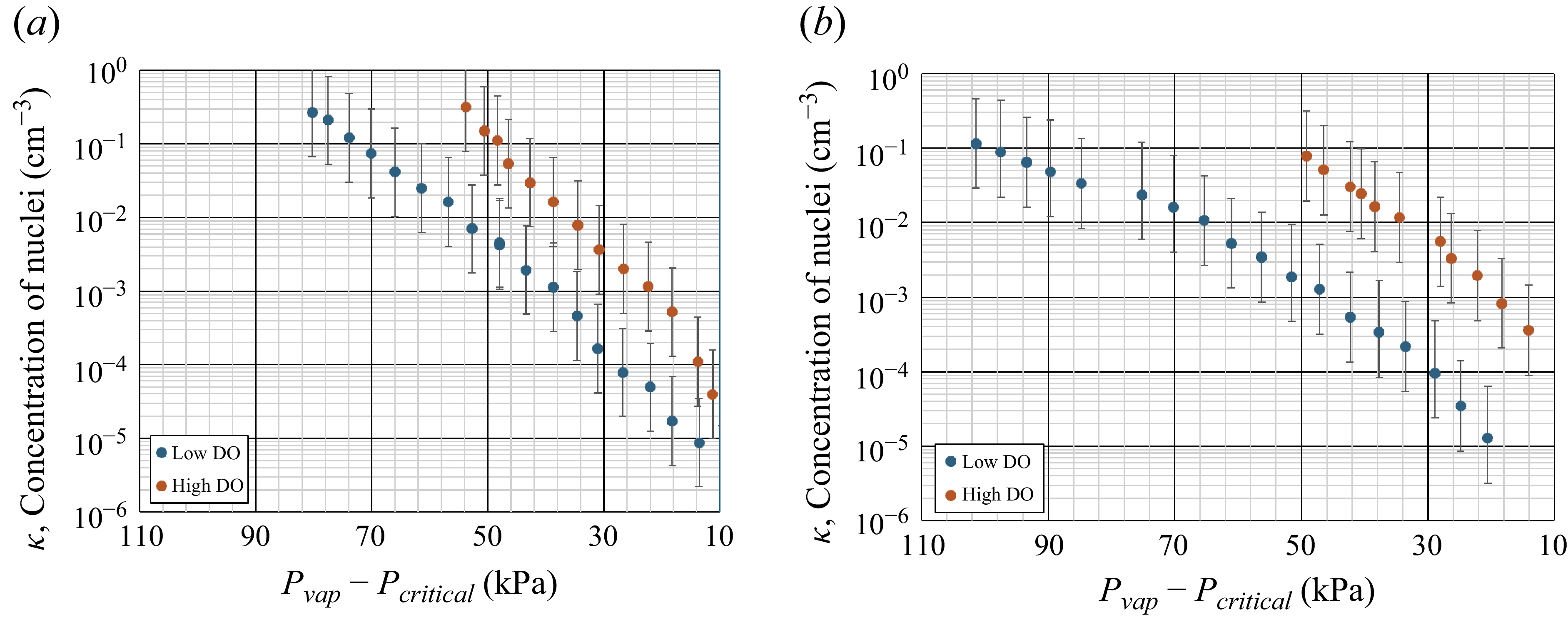


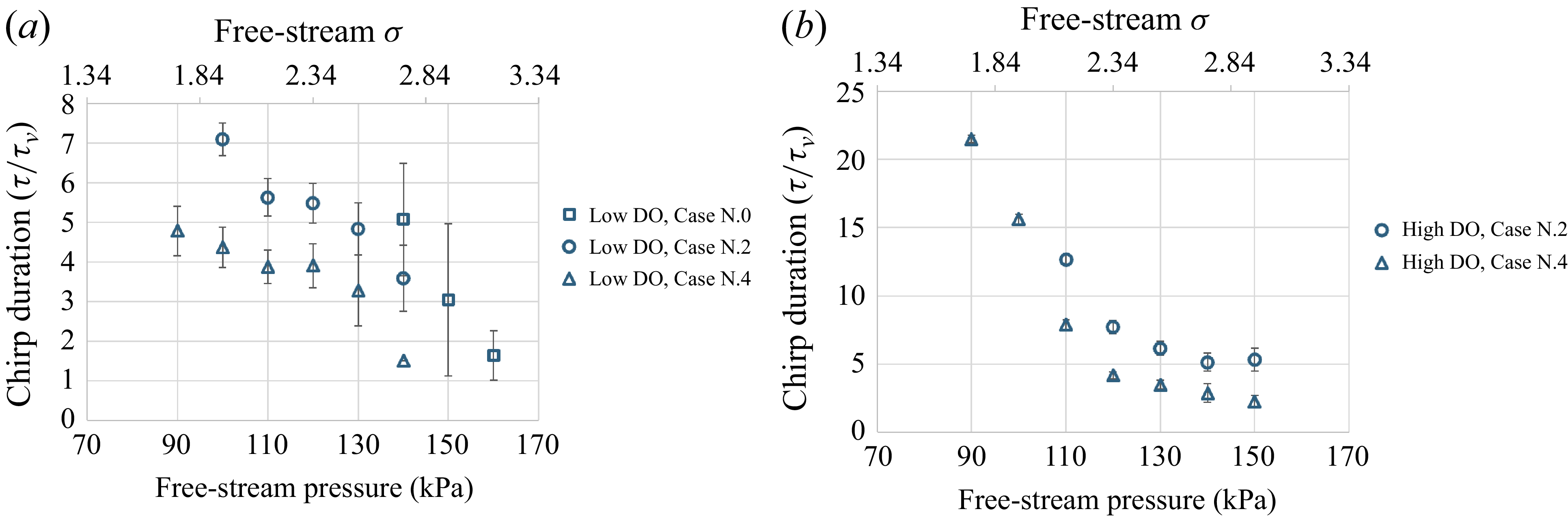


 Open access