2.1. Numerical method

In the present study, the flow was solved by DNS using the open-source software packages OpenFOAM (www.openfoam.org) and Nektar++ (Cantwell et al. Reference Cantwell2015). The governing equations were the continuity and incompressible Navier–Stokes equations:

(2.1)\begin{gather}\frac{{\partial {u_i}}}{{\partial {x_i}}} = 0,\end{gather}

(2.2)\begin{gather}\frac{{\partial {u_i}}}{{\partial t}} + {u_j}\frac{{\partial {u_i}}}{{\partial {x_j}}} ={-} \frac{1}{\rho }\frac{{\partial p}}{{\partial {x_i}}} + \nu \frac{{{\partial ^2}{u_i}}}{{\partial {x_j}\partial {x_j}}},\end{gather}

where (x ₁, x ₂, x ₃) = (x, y, z) are Cartesian coordinates, u_i is the velocity component in the direction x_i, t is time, ρ is fluid density, p is pressure and ν is kinematic viscosity.

For the OpenFOAM model, (2.1)–(2.2) were solved by the finite volume method (FVM) and the Pressure Implicit with Splitting of Operators (PISO) algorithm (Issa Reference Issa1986). The convection, diffusion and time derivative terms were discretized respectively using a fourth-order cubic scheme, a second-order linear scheme, and a blended scheme consisting of the second-order Crank–Nicolson scheme and a first-order Euler implicit scheme. Specifically, since the fully centred and second-order Crank–Nicolson scheme is often unstable for complex flows (as was the case for a square cylinder studied by Jiang and Cheng (Reference Jiang and Cheng2018)), it is necessary to ‘off-centre’ the scheme to stabilize it while retaining greater temporal accuracy than the first-order Euler-implicit scheme (Vukčević, Jasak & Malenica Reference Vukčević, Jasak and Malenica2016; Pedersen et al. Reference Pedersen, Larsen, Bredmose and Jasak2017; Seng, Monroy & Malenica Reference Seng, Monroy and Malenica2017). Following Jiang & Cheng (Reference Jiang and Cheng2018), an off-centring coefficient of 0.5 (a value of 1.0 represents the Crank–Nicolson scheme while 0 represents the Euler-implicit scheme) was used in this study as a compromise between accuracy and stability. To solve the linear algebraic equations, the generalised geometric-algebraic multi-grid (GAMG) solver was used to solve the pressure, while the Gauss–Seidel smooth solver was used to solve the velocity components. For each time step, the tolerance for the pressure and velocity components was set to 10⁻⁷. More details on the above-mentioned schemes and solvers can be found from Moukalled, Mangani & Darwish (Reference Moukalled, Mangani and Darwish2015).

For the Nektar++ model, (2.1) and (2.2) were solved by the unsteady incompressible Navier–Stokes solver embedded in the code. A velocity-correction splitting scheme (Karniadakis, Israeli & Orszag Reference Karniadakis, Israeli and Orszag1991) was used to decouple the pressure and velocity fields. The time discretisation was achieved using a second-order implicit–explicit time-stepping scheme described by Vos et al. (Reference Vos, Eskilsson, Bolis, Chun, Kirby and Sherwin2011). A high-order continuous Galerkin projection (Karniadakis & Sherwin Reference Karniadakis and Sherwin2005) was used. The global linear system was solved by using a parallel Cholesky factorisation based on the XX^T library, and the static condensation technique was applied repeatedly to reduce the system size and to improve the computational efficiency (Karniadakis & Sherwin Reference Karniadakis and Sherwin2005). For each time step, the tolerance for the pressure and velocity components was set to 10⁻⁸. More details on the Nektar++ approach can be found from Karniadakis & Sherwin (Reference Karniadakis and Sherwin2005), Cantwell et al. (Reference Cantwell2015) and Moxey et al. (Reference Moxey2020).

The present 2-D DNS was mainly conducted using the OpenFOAM model. An advantage of the OpenFOAM model is that, by deliberately coarsening the mesh at a specific streamwise location in the wake, the wake structure beyond this location is quickly annihilated and its effect on the flow upstream of this location is eliminated artificially, which is beneficial to the analysis in § 3.2. In addition to the OpenFOAM simulations, some of the 2-D cases were also simulated using Nektar++, for the purposes of (i) cross-checking the numerical results predicted by the two models (reported in § 2.3) and (ii) obtaining the 2-D base flow for the Floquet stability analysis (to be performed under the framework of Nektar++ in § 4.1).

The present 3-D DNS was conducted using the Nektar++ model only. Specifically, a high-order spectral/hp element method (Karniadakis & Sherwin Reference Karniadakis and Sherwin2005) was used for the x–y plane perpendicular to the spanwise (z-) direction, while a Fourier expansion (Karniadakis Reference Karniadakis1990) was used in the spanwise direction owing to the spanwise homogeneity of the cylinder. This approach offers a greater computational efficiency than conventional FVM and similar approaches (Cantwell et al. Reference Cantwell2015; Moxey et al. Reference Moxey2020), as illustrated by e.g. a comparison of Nektar++ and OpenFOAM in the simulation of flow past a circular cylinder (Jiang & Cheng Reference Jiang and Cheng2021).

2.2. Computational domain and mesh

For both the OpenFOAM and Nektar++ models, a rectangular computational domain was used in the x–y plane, with the centre of the cylinder located at (x, y) = (0, 0) (figure 2a). The computational domain size from the cylinder centre to the inlet and each of the transverse sides was 60D, while the domain size in the wake was extended to 200D to resolve the far-wake patterns.

Figure 2.

Computational domain and mesh for AR = 0.375. (a) Schematic model of the computational domain (not to scale), (b) close-up view of the OpenFOAM mesh near the cylinder and (c) close-up view of the Nektar++ macro-element mesh near the cylinder.

The boundary conditions for the computational domain were specified as follows. The velocity boundary conditions included a uniform velocity U in the x-direction for the inlet, a Neumann condition (i.e. zero normal gradient) for the outlet, symmetry boundary conditions for the top and bottom boundaries, and a no-slip condition on the cylinder surface. The pressure boundary conditions included a reference value of zero at the outlet, and a Neumann condition for all other boundaries. For the Nektar++ model, the Neumann condition for the pressure employed a high-order form (Karniadakis et al. Reference Karniadakis, Israeli and Orszag1991). For the 3-D DNS, periodic boundary conditions were applied to the two lateral boundaries perpendicular to the spanwise direction. At the beginning of a simulation, the internal flow followed an impulsive start. The time step size was chosen based on a Courant–Friedrichs–Lewy (CFL) limit of 0.5.

For the OpenFOAM model, the computational meshes for flow past rectangular cylinders with various AR values were modified from the one used by Jiang et al. (Reference Jiang, Cheng and An2018) for a square cylinder (i.e. AR = 1.0). Specifically, the cell size at the two leading edges of the cylinder (where largest pressure gradients took place) was 0.005D × 0.005D, the number of cells along the front/rear side of the cylinder was 52, while the number of cells along the top/bottom side varied from 2 for AR = 0.01 to 46 for AR = 0.625. The cell expansion ratio in the whole domain was kept below 1.1. To capture detailed near-wake and far-wake flow structures, a relatively high mesh resolution was used in the entire wake region by specifying the streamwise mesh sizes along the wake centreline (y = 0) varying linearly from Δx = 0.05D at 0.5D downstream of the rear surface of the cylinder to Δx = 0.125D at x/D = 200. The total number of cells in the computational domain varied from 516,006 for AR = 0.01 to 521,798 for AR = 0.625. Figure 2(b) shows a close-up view of the mesh near the cylinder for AR = 0.375.

For the Nektar++ model, the general topological pattern of the computational mesh in the x–y plane remained similar to that for the OpenFOAM model, but the resolution of the macro-element mesh was coarsened (figure 2c versus figure 2b). Specifically, the macro-element size at the two leading edges of the cylinder was 0.03D × 0.03D, the number of cells along the front/rear side of the cylinder was 16, while the number of cells along the top/bottom side varied from 2 for AR = 0.0625 to 12 for AR = 0.625. The expansion ratio of the macro-elements was kept below 1.25. For the 2-D DNS, the macro-element sizes along the wake centreline increased linearly from Δx = 0.2D at 1D downstream of the rear surface of the cylinder to Δx = 0.7D at x/D = 200. For the 3-D DNS, the outlet was truncated at x/D = 40, while the cell expansion ratio was unchanged. The reason for the truncation at x/D = 40 was that the 3-D DNS focused on (i) the interaction between the 2-D and 3-D wake transitions, which occurred at the immediate near wake, and (ii) the corresponding influence on the hydrodynamic forces, where the present 2-D DNS found that the 2-D wake transition induced less than 1 % influence on the hydrodynamic forces when the transition occurred at x/D > 39 (§ 3.2), and the interaction between the 2-D and 3-D wake transitions may further weaken the influence on the hydrodynamic forces (§ 4), such that the wake length up to x/D = 40 was sufficient for an accurate determination of the hydrodynamic forces. The total number of macro-elements in the computational domain was ~40,000 for the 2-D DNS (up to x/D = 200) and was reduced to ~15 000 for the 3-D DNS (up to x = 40D). Each macro-element was then subdivided using 4th-order Lagrange polynomials on the Gauss–Lobatto–Legendre points for the quadrilateral expansion (denoted N_p = 4). The 3-D mesh used 128 Fourier planes over a spanwise domain length L_z/D = 15 to resolve the 3-D wake structures. The L_z/D followed that used by Jiang et al. (Reference Jiang, Cheng and An2018) for AR = 1.0 (as the largest spanwise wavelength for the 3-D wake instability modes does not vary strongly with AR; see figure 15b), while the adequacy of the spanwise resolution will be examined in § 2.3.

2.3. Mesh convergence study

First, the 2-D mesh used by the OpenFOAM model (called the standard mesh) was examined with two variations: (i) a mesh refined in both the x- and y-directions with doubled numbers of cells in both directions (i.e. four times the number of cells compared with the standard mesh) and a halved time step size to satisfy the same CFL limit, and (ii) a mesh with an enlarged domain size from the cylinder centre to the inlet, top and bottom boundaries (from 60D to 120D). Table 1 lists the cases and numerical results obtained with the three meshes. The mesh convergence check was mainly conducted at Re = 200, the largest Re simulated by the OpenFOAM model. The numerical results listed in table 1 included the Strouhal number St, the time-averaged drag coefficient $\overline {{C_D}}$ and the root-mean-square lift coefficient ${C^{\prime}_L}$, which are calculated as

(2.3)\begin{gather}St = \frac{{{f_L}D}}{U},\end{gather}

(2.4)\begin{gather}{C_D} = \frac{{{F_D}}}{{{\textstyle{1 \over 2}}\rho {U^2}D{L_z}}},\end{gather}

(2.5)\begin{gather}{C_L} = \frac{{{F_L}}}{{{\textstyle{1 \over 2}}\rho {U^2}D{L_z}}},\end{gather}

where F_D and F_L are the drag and lift forces on the cylinder, respectively, and f_L is the frequency of the fluctuating lift force. The time-averaged drag and lift coefficients are denoted as $\overline {{C_D}}$ and $\overline {{C_L}}$, respectively. The root-mean-square lift coefficient ${C^{\prime}_L}$ is calculated as

(2.6)\begin{equation}{C^{\prime}_L} = \sqrt {\frac{1}{N}\sum\limits_{i = 1}^N {{{({C_{L,i}} - \overline {{C_L}} )}^2}} } ,\end{equation}

where N is the number of values in the time history of ${C_L}$. Table 1 also summarises the streamwise locations for the first transition (x_{tr 1}/D) and second transition (x_{tr 2}/D) in the wake.

Table 1.

Mesh convergence check of several 2-D cases.

As shown in table 1, for each case, the hydrodynamic forces and the transition locations predicted by the two variation meshes were very close to those predicted by the standard mesh (the relative differences in the hydrodynamic forces, the first and the second transition locations were generally within 1.5 %, 1 % and 3 %, respectively). The two cases with AR = 0.125 were also simulated by the Nektar++ model, and the numerical results are also listed in table 1. The close agreement in the results predicted with N_p = 3 and 4 suggested that mesh convergence was reached. The close agreement in the results predicted by Nektar++ and OpenFOAM suggested that both numerical models were reliable.

The present results were also validated against those reported in the literature. As shown later on in figure 7(g,h), the entire St–Re and $\overline {{C_D}} - Re$ relationships for AR = 0.01 and Re = 50–200 calculated with the standard mesh were within 2 % of those calculated by Thompson et al. (Reference Thompson, Radi, Rao, Sheridan and Hourigan2014) for AR = 0.

For the 3-D mesh, the spanwise mesh resolution used by the Nektar++ model was examined based on the case (AR, Re) = (0.125, 280), where Re = 280 was the largest Re examined in this study, and the 3-D vortex structures were expected to be the finest. Table 2 shows that, after increasing the number of Fourier planes from 128 to 192, the relative differences in the hydrodynamic forces were well within 1 %.

Table 2.

Mesh convergence check for the 3-D case of (AR, Re) = (0.125, 280).

Based on the mesh convergence study reported in this section, the standard meshes introduced in § 2.2 were considered adequate and were used in the present study.

3.1. Two-dimensional wake transition

The 2-D wake transitions and their direct influence on the hydrodynamic forces on the cylinder are investigated first. Figure 3 summarises the streamwise locations for the first and second transitions for the cases with various AR and Re combinations. In general, the two transition locations move closer to the cylinder with increasing Re and decreasing AR. The results for AR > 0.5 are not shown in figure 3, since the transition locations are relatively far away from the cylinder. For example, for AR = 0.625 and Re ≤ 200, the first transition occurs at x/D ≥ 17, while the second transition occurs well beyond x/D = 70.

Figure 3.

Streamwise locations of the two transitions for the cases with various AR and Re combinations.

Based on the assumptions of inviscid flow and point vortex, Durgin & Karlsson (Reference Durgin and Karlsson1971) and Karasudani & Funakoshi (Reference Karasudani and Funakoshi1994) showed that the first transition in the wake of a circular cylinder occurred when the spacing ratio of the vortices, defined as the vertical distance (h) to the horizontal distance (a) between the adjacent vortices (see the inset of figure 4a) exceeded a critical value of 0.365. Thompson et al. (Reference Thompson, Radi, Rao, Sheridan and Hourigan2014) showed that this criterion was also broadly applicable to an elliptical cylinder. In the present study, this criterion is re-examined for the case of a rectangular cylinder. Figure 4 shows the streamwise variation of the spacing ratio h/a for the cases with various AR and Re combinations. The vortex centre of each vortex is determined at the location of peak vorticity. Jiang & Cheng (Reference Jiang and Cheng2019) showed based on the laminar wake of a circular cylinder that prior to the second transition, the centres of positive and negative vortices follow two clear trajectories on the two sides of the wake centreline. Therefore, the vortex trajectories and thus the streamwise variation of h/a can be determined by an instantaneous vortex field at an arbitrary phase. In figure 4, the solid dot on each curve marks the streamwise location for the first transition determined in figure 3. The corresponding h/a values span a range of 0.33 to 0.50. The moderate discrepancies between the present h/a values and the critical condition of h/a = 0.365 (marked by the horizontal dashed line in figure 4) proposed by Durgin & Karlsson (Reference Durgin and Karlsson1971) and Karasudani & Funakoshi (Reference Karasudani and Funakoshi1994) may be attributed to the two assumptions used for the determination of h/a = 0.365. For example, Karasudani & Funakoshi (Reference Karasudani and Funakoshi1994) suggested that for vortices of fairly large areas (in contrast to the assumption of point vortex), the critical h/a may be larger than 0.365 (consistent with the present results of Re = 100 and 140 shown in figure 4b,c). Regardless of the exact critical value of h/a, the h/a–x/D relationships shown in figure 4 suggest that h/a increases with increasing Re and decreasing AR, which physically explains the upstream movement of the first transition with increasing Re and decreasing AR (figure 3).

Figure 4.

Streamwise variation of the spacing ratio h/a for the cases with various AR and Re combinations:(a) Re = 60; (b) Re = 100; and (c) Re = 140. The horizontal dashed line marks the critical value of 0.365 given by Durgin & Karlsson (Reference Durgin and Karlsson1971) and Karasudani & Funakoshi (Reference Karasudani and Funakoshi1994). For the case (Re, AR) = (60, 0.5), it is difficult to determine the location of the first transition based on the method illustrated in figure 1, so the solid dot is omitted.

The above analysis shows that the streamwise location of the first transition is governed by the spatial arrangement of the vortices. However, the influence of the strengths of the vortices is minor. For example, figure 5 shows the strengths of the vortices for the cases with Re = 100 and various AR values, quantified using both the peak vorticity (figure 5a) and circulation (figure 5b) within each vortex. The circulation within each vortex is calculated as

(3.1)\begin{equation}\varGamma = \int_\varOmega {{\omega _z}\,\textrm{d}\varOmega } ,\end{equation}

where $\varOmega$ is the area of the vortex, determined as the region within which the vorticity is larger than 30 % of the peak vorticity of the vortex. As shown in figure 5, prior to the first transition, the vortex strengths for different AR values are similar, which suggests that vortex strength is not a major factor governing the streamwise location of the first transition.

Figure 5.

Strengths of the vortices for the cases with Re = 100 and various AR values, quantified by (a) the peak vorticity in a vortex and (b) the circulation within a vortex.

As the wake transitions to the two-layered pattern, the significant difference in the streamwise velocity between the outer and calm regions forms a strong shear layer at each side of the wake centreline, which results in strong convective instability of the flow and consequently the transition, further downstream, to the secondary vortex street through flapping/waviness of the two shear layers (Kumar & Mittal Reference Kumar and Mittal2012; Jiang Reference Jiang2021). Figure 6 quantifies the streamwise variation of the maximum shear rate of the shear layers for various cases. The maximum shear rate at a specific streamwise location is determined using the time-averaged streamwise velocity profile sampled along the transverse direction. The maximum shear rate displays a gradual increase near the location of the first transition (as the transition is a gradual process), followed by a mild decrease over the two-layered wake region, and a steeper decrease near the location of the second transition as the calm region is terminated. With the increase in Re and decrease in AR, the first transition occurs closer to the cylinder (figures 3 and 6), and so does the increase in the maximum shear rate (figure 6). In addition, figure 6(a) shows that with the increase in Re, the maximum shear rate increases to a higher level over the two-layered wake region. Therefore, with increasing Re and decreasing AR, the shear-induced convective instability is stronger and the transient growth of the disturbance develops faster over the same range of downstream distance, such that the second transition also occurs closer to the cylinder (figures 3 and 6). An exception is the cases with AR = 0.5 and Re ≥ 170, where the maximum shear rate over the two-layered wake region reaches higher levels than that of AR ≤ 0.375 (also observed in figure 6b), such that the transient growth of the disturbance may develop faster to allow for an earlier second transition than that for AR = 0.375 (figure 3).

Figure 6.

Streamwise variation of the maximum shear rate of the shear layers for (a) the cases with AR = 0.125 and various Re values, and (b) the cases with Re = 160 and various AR values. The downstream end of each curve is the location of the second transition.

3.2. Direct influence of 2-D wake transition on the hydrodynamic forces

For the cases with various AR and Re combinations, the St, $\overline {{C_D}}$ and ${C^{\prime}_L}$ values determined from the fully developed 2-D flows are summarised in figure 7 (curve I in each panel). Figure 7(j,k) also shows the St and $\overline {{C_D}}$ values for a flat plate (i.e. AR = 0) predicted by Thompson et al. (Reference Thompson, Radi, Rao, Sheridan and Hourigan2014), which agreed well the present results of AR = 0.01. An interesting phenomenon observed in figure 7 is that the variation in the hydrodynamic forces with Re contains a downward bend and subsequently an upward bend over the range of Re = 50–200. It is suspected that the first and second bends are induced by the first and second transitions, respectively. However, the possible link between one wake transition and one bend is not straightforward, since both wake transitions are at play and the hydrodynamic forces are influenced as a whole. Therefore, specifically designed numerical cases are used in the present study to decompose the influence of the first and second transitions.

Figure 7.

St–Re, $\overline {{C_D}} - Re$ and ${C^{\prime}_L} - Re$ relationships for flow past a rectangular cylinder.

First, the influence of the second transition is quantified by additional numerical cases with an artificial horizontal slip plate (with slip boundary conditions ∂u_x/∂y = 0, u_y = 0 and ∂p/∂y = 0) of zero-thickness placed at the wake centreline and x/D ≥ 10.5. The use of such a slip plate would not affect the first transition that occurs at $x/D\lesssim 10$, but would eliminate potential interaction between the upper and lower shear layers (and the two rows of vortices) further downstream. Without such interaction, the convective instability and transient growth of perturbation energy with distance downstream are significantly weakened (Jiang Reference Jiang2021), and therefore the second transition is suppressed (figure 12c versus figure 12a in § 3.3). It was also tested based on the case (AR, Re) = (0.125, 150) that by changing the starting point of the slip plate from x/D = 10.5 to x/D = 15.5, the variations in the hydrodynamic forces were within 0.2 %, i.e. the results were unaffected by the starting point of the slip plate, as long as the vortex merging event was eliminated. The DNS results with the slip plate are shown in figure 7 as curve II. The influence of the second transition on the hydrodynamic forces is thus isolated as the upward bend from curve II to curve I (figure 7).

For the cases with various AR and Re combinations, the relationship between the location of the second transition (figure 3) and the increase in St, $\overline {{C_D}}$ and ${C^{\prime}_L}$ due to the second transition (from curve II to curve I in figure 7) is plotted in figure 8. The increase in St, $\overline {{C_D}}$ and ${C^{\prime}_L}$ is calculated as

(3.2)\begin{equation}\textrm{Increase}\;(\%) = \frac{{\textrm{Result}\;\textrm{on}\;\textrm{curve}\;\textrm{I } - \textrm{Result}\;\textrm{on}\;\textrm{curve}\;\textrm{II}}}{{\textrm{Result}\;\textrm{on}\;\textrm{curve}\;\textrm{II}}} \times 100\,\%.\end{equation}

As shown in figure 8, the results of AR = 0.01–0.375 collapse well onto exponential fittings. Noticeable increases in the hydrodynamic forces on the cylinder are observed even when the second transition occurs relatively far away from the cylinder. For example, the hydrodynamic forces increase by 1 % and 10 % when the second transition occurs at x/D = 39 and 16, respectively.

Figure 8.

Relationship between the location of the second transition and the increase in (a) St, (b) $\overline {{C_D}}$ and(c) ${C^{\prime}_L}$ due to the second transition.

To further exclude the first transition (and naturally also the second transition), the following two methods are used. Method 1 eliminates potential development of the first transition, while method 2 records the results prior to the development of the first transition.

1. (i) Method 1. Section 3.1 shows that the first transition arises from the downstream evolution of the spatial arrangement of the vortices until h/a exceeds a critical value. To exclude the first transition that develops downstream of the critical h/a, the computational mesh is modified to preserve a high wake resolution for only x/D = 0–3. For x/D > 3, the cell expansion ratio in the horizontal direction is modified from 1.000377 to 1.1 so as to phase out the vortices rapidly. In this way, the first transition that could have occurred at x/D ≳ 3 is eliminated (figure 12e versus figure 12a,c in § 3.3). For the cases with AR = 0.375, the converged hydrodynamic forces calculated by method 1 are shown in figure 7(a–c) as curve IV.

2. (ii) Method 2. Because the development of ‘regular Kármán vortex street → the first transition → the second transition’ is sequential and irreversible, this method should start from an initial condition which allows for natural development of the regular Kármán vortex street (prior to the first and second transitions). To this purpose, an impulsive start is used as the initial condition, for which a regular Kármán vortex street always develops first. As an example, figure 9 illustrates the time evolution of the vorticity field over different stages for a typical case (AR, Re) = (0.375, 200). With the evolution in time, the wake displays a regular Kármán vortex street in figure 9(b), followed by the emergence of the two-layered pattern at t* (= tU/D) ~ 82 and x/D ~ 10 (figure 9c), and the emergence of vortex merging and the second transition at t* ~ 110 and x/D ~ 10 (figure 9d). Figure 10 shows the corresponding time evolution of the St, $\overline {{C_D}}$ and ${C^{\prime}_L}$ values. Each point in figure 10 is determined by calculating the quantity based on one vortex shedding period. As shown in figure 10, the three quantities peak at t* ~ 70, which corresponds to the regular Kármán vortex street in figure 9(b) and prior to the emergence of the first and second transitions in figure 9(c,d). Therefore, the largest St, $\overline {{C_D}}$ and ${C^{\prime}_L}$ values over the time evolution are considered as the results without the influence of the first and second transitions. These results are shown in figure 7 as curve III.

Figure 9.

Time evolution of the vorticity field for the case (AR, Re) = (0.375, 200): (a) t* = 28; (b) t* = 72; (c) t* = 82; and (d) t* = 114. The two transition locations for the fully developed flow are marked by the vertical dashed lines.

Figure 10.

Time evolution of the St, $\overline {{C_D}}$ and ${C^{\prime}_L}$ values for the case (AR, Re) = (0.375, 200).

As shown in figure 7(a–c), curve III predicted by method 2 and curve IV predicted by method 1 agree well, although curve III is slightly lower than curve IV. The slight difference is because in method 2, the transient state prior to the emergence of the first transition persists for only a short period of time, and the largest St, $\overline {{C_D}}$ and ${C^{\prime}_L}$ values captured over the time evolution may not be as large as the theoretical values for a fully developed Kármán vortex street (as predicted by method 1).

Nevertheless, for the cases with AR ≤ 0.125, method 1 may not be applicable because the first transition occurs increasingly closer to the cylinder with decreasing AR (figure 3), and consequently the first transition cannot be excluded in the simulation, since a relatively fine mesh is still required in the immediate neighbourhood of the cylinder and the cell expansion ratio is finite (generally less than 1.1). Therefore, only method 2 is used in figure 7(d–i) to show approximately the results excluding the first transition. The influence of the first transition on the hydrodynamic forces is thus isolated as the downward bend from curve III to curve II (figure 7).

For the cases with various AR and Re combinations, the relationship between the location of the first transition (figure 3) and the reduction in St, $\overline {{C_D}}$ and ${C^{\prime}_L}$ due to the first transition (from curve III to curve II in figure 7) is plotted in figure 11. The reduction in St, $\overline {{C_D}}$ and ${C^{\prime}_L}$ is calculated as

(3.3)\begin{equation}\textrm{Reduction}\;(\%) = \frac{{\textrm{Result}\;\textrm{on}\;\textrm{curve}\;\textrm{III}\textrm{ } - \textrm{Result}\;\textrm{on}\;\textrm{curve}\;\textrm{II}}}{{\textrm{Result}\;\textrm{on}\;\textrm{curve}\;\textrm{III}}} \times 100\,\%.\end{equation}

Figure 11.

Relationship between the location of the first transition and the reduction in (a) St, (b) $\overline {{C_D}}$ and (c) ${C^{\prime}_L}$ due to the first transition.

As shown in figure 11, the results of AR = 0.01–0.375 collapse well onto logistic fittings. The reductions in the hydrodynamic forces become noticeable, e.g. >1 %, when the first transition occurs within x/D ~ 12. As the first transition moves closer to the cylinder, considerable reductions (up to ~35 %) in the hydrodynamic forces on the cylinder may be observed.

The above findings have implications on the choice of the wake resolution for numerical studies, because it is demonstrated that even relatively far-wake flow patterns may affect the hydrodynamic forces on the cylinder. For the simulation of flow past a circular/square cylinder, a high wake resolution of only a few cylinder diameters may be sufficient (e.g. Jiang et al. Reference Jiang, Cheng, Draper, An and Tong2016, Reference Jiang, Cheng and An2018), because the 2-D wake transitions are sufficiently far away from the cylinder (e.g. x/D = 28 and 75 for the first and second transitions in the wake of a circular cylinder at Re = 250, and x/D = 51 for the first transition in the wake of a square cylinder at Re = 250) and would not induce noticeable influence on the hydrodynamic forces on the cylinder. However, for bluff-body flows with the first transition occurring at $x/D\lesssim 12$ and/or the second transition occurring at $x/D\lesssim 39$, the 2-D transition needs to be incorporated to produce correct hydrodynamic forces and near-wake flow patterns.

3.3. Physical mechanisms for the variations in the hydrodynamic forces

The case (AR, Re) = (0.375, 200) is used here again to explain the physical mechanisms for the variations in the hydrodynamic forces by the two transitions. In addition to the standard case with a high wake resolution for x/D = 0–200 (figure 12a), two variation cases are considered.

1. (i) Variation case 1: A wake slip plate is used for x/D = 10.5–200 to exclude the second transition (figure 12c).

2. (ii) Variation case 2: A high wake resolution is used for only x/D = 0–3 to exclude both the first and second transitions (figure 12e).

Figure 12.

Flow characteristics for the case (AR, Re) = (0.375, 200): (a) fully developed instantaneous vorticity field for the standard case; (b) time-averaged pressure field for the standard case; (c) fully developed instantaneous vorticity field for variation case 1; (d) time-averaged pressure field for variation case 1; (e) fully developed instantaneous vorticity field for variation case 2; and (f) time-averaged pressure field for variation case 2. The vertical dashed lines in panels (a–d) mark the locations for the first and second transitions.

The drag and lift forces on the cylinder consist of pressure and viscous components. By separating the pressure and viscous components of the $\overline {{C_D}}$ and ${C^{\prime}_L}$ values, it is found that the reductions in the $\overline {{C_D}}$ and ${C^{\prime}_L}$ values from variation case 2 to case 1 (i.e. due to the first transition) are 100 % and 87 % contributed by the pressure component, respectively, while the increases in the $\overline {{C_D}}$ and ${C^{\prime}_L}$ values from variation case 1 to the standard case (i.e. due to the second transition) are also 100 % and 87 % contributed by the pressure component, respectively.

Since the variations in the forces are primarily contributed by the pressure component, the pressure distributions of the above-mentioned three cases are examined. Figure 12(b,d,f) shows the time-averaged pressure fields for the three cases. A comparison between variation case 1 (figure 12d) and case 2 (figure 12f) shows that the occurrence of the first transition induces a significant reduction in the magnitude of the negative pressure at the location of the first transition, especially near the wake centreline, which is because the occurrence of the first transition induces a ‘calm region’ near the wake centreline.

Figure 13(a,b) shows the variations of the time-averaged pressure coefficient along the wake centreline and on the cylinder surface. The pressure coefficient is defined as

(3.4)\begin{equation}{C_p} = \frac{{p - {p_\infty }}}{{{\textstyle{1 \over 2}}\rho {U^2}}},\end{equation}

where p is the pressure at a specific point and p _∞ is the reference pressure sampled at the location of the inlet boundary. A comparison between the variation cases 1 and 2 shows that the reduction in the magnitude of the negative pressure (i.e. reduction in $|{\overline {{C_p}} } |$) at the location of the first transition extends its effect back to the cylinder surface (figure 13a), in particular on the upper, rear and lower surfaces of the cylinder (figure 13b). The reduction in $|{\overline {{C_p}} } |$ on the upper, rear and lower surfaces of the cylinder is the direct cause for the reduction in $\overline {{C_D}}$.

Figure 13.

Pressure distribution for the case (AR, Re) = (0.375, 200): (a) time-averaged pressure coefficient along the wake centreline; and (b) time-averaged pressure coefficient on the cylinder surface.

Similar to the reduction in $\overline {{C_D}}$ due to the reduction in $|{\overline {{C_p}} } |$ in the wake as a result of the first transition, the slight increase in $\overline {{C_D}}$ as a result of the second transition is due to the slight increase in $|{\overline {{C_p}} } |$ at the location of the second transition (the standard case versus variation case 1 in figure 13a), owing to the termination of the calm region (figure 1b,c) as the flow reoccupies the wake centreline in the secondary vortex street (figure 12a). A comparison of variation case 1 (figure 12c) and the standard case (figure 12a) shows that without the second transition, the calm region extends further downstream. A longer calm region would have a stronger effect in reducing $|{\overline {{C_p}} } |$ in the wake.

The reduction in $|{\overline {{C_p}} } |$ in the wake also reduces the strength of the vortices in the wake, which is quantified in figure 14 by the streamwise evolution of the peak vorticity of the vortices. The reduction in the vortex strength as a result of the first transition would reduce the fluctuating lift on the cylinder, since the alternate formation of the vortices and low-pressure regions on the two sides of the cylinder is the cause of fluctuating lift.

Figure 14.

Streamwise evolution of the peak vorticity of the vortices for the case (AR, Re) = (0.375, 200).

As for the variation in St, Roshko (Reference Roshko1955) suggested that the Strouhal number of a bluff body scaled better on the velocity at separation (U_s) and the wake width (D′), rather than simply on U and D. For the three cases examined here, the variations in the wake width (as defined by Jiang & Cheng (Reference Jiang and Cheng2017)) are less than 2 %. However, the velocity at separation, as approximately represented by the largest velocity in the time-averaged streamwise velocity profile sampled along the y-direction at x/D = 0.1875 (the rear surface of the cylinder), displays an 11.7 % reduction from case 2 to case 1 (i.e. due to the first transition) and a 3.4 % increase from case 1 to the standard case (i.e. due to the second transition), which are proportional to the variations in St shown in figure 7(a), namely an 18.9 % reduction and a 5.8 % increase, respectively. The increase/decrease in the velocity at separation is consistent with the increase/decrease in $|{\overline {{C_p}} } |$ in the near wake (figure 13).

4.1. Summary of the 3-D wake instability modes

In the 3-D flow regimes, the interactions between the 2-D and 3-D wake transitions/structures may further alter the hydrodynamic forces on the cylinder. In the literature, the critical Re values for the 3-D wake transition of a bluff body have been routinely determined by the Floquet stability analysis. However, the Floquet analysis for a rectangular cylinder differs from the conventional Floquet analysis for e.g. a circular or a square cylinder, in that the 2-D base flow for a thin rectangular cylinder may not be time-periodic, because the aperiodic emergence of the secondary vortices may occur relatively close to the cylinder (see figure 3), which restricts the applicability of the Floquet analysis. Although Choi & Yang (Reference Choi and Yang2014) reported the critical Re and the corresponding spanwise wavelength (λ/D) for the 3-D wake instability modes of rectangular cylinders based on the Floquet analysis (figure 15), they did not report whether and how they took into account the aperiodic emergence of the secondary vortices in the base flow. Therefore, the Floquet analysis for the rectangular cylinders is re-examined here, with a particular care on the periodicity of the base flow.

Figure 15.

Floquet analysis results for various AR values: (a) critical Re for the 3-D wake instability modes; and (b) critical λ/D for these modes.

In the present study, a time-periodic base flow is established by performing phase average of the aperiodic 2-D flow over 80 primary vortex shedding periods (T). The adequacy of 80T for the phase average is confirmed by testing 40T, 80T and 160T for the Floquet analysis of the case (AR, Re) = (0.5, 200) at a spanwise wavenumber β (= 2${\rm \pi}$/λ) of 1.4 (within the range of a conventional mode A instability), where the Floquet multiplier μ predicted by the three time ranges differ by less than 0.01 %. Based on the phase-averaged time-periodic base flow, the present Floquet analysis results are also summarised in figure 15. The critical Re and λ/D are determined by a linear interpolation of the Floquet analysis results with an Re interval of 3, while the critical λ/D for each Re is determined by a fourth-order polynomial interpolation of the |μ| − β relationship. As shown in figure 15, the present Floquet analysis results agree well with those reported by Choi & Yang (Reference Choi and Yang2014). Although figure 15 seems to be a mere reproduction of the previous results of Choi & Yang (Reference Choi and Yang2014), a strict Floquet analysis with a time-periodic base flow is a requisite for determining the wake instability modes accurately, which then helps to determine the (AR, Re) values for the expensive 3-D DNS cases.

According to the Floquet analysis results shown in figure 15, two AR values, 0.5 and 0.125, are of particular interest.

1. (i) The conventional sequence of wake instability modes ‘A → B → QP (a quasi-periodic mode)’ observed for a square cylinder (Blackburn & Lopez Reference Blackburn and Lopez2003; Sheard, Fitzgerald & Ryan Reference Sheard, Fitzgerald and Ryan2009) and a rectangular cylinder with AR = 0.625–1 (figure 15) is not observed for AR ≤ 0.5. In particular, for AR = 0.5, mode A is the only instability mode identified by the Floquet analysis up to Re = 300. With the absence of the modes B and QP instabilities for AR = 0.5, it would be interesting to examine through 3-D DNS if the actual 3-D wake transition route to chaos/turbulence would be different from the conventional wake transition process ‘mode A → mode swapping between modes A and B → increasingly chaotic mode B’ for a square cylinder (Jiang et al. Reference Jiang, Cheng and An2018).

2. (ii) For AR = 0.125 and increasing Re, the flow is first unstable to a mode A instability, followed by a re-stabilisation to a 2-D regime and subsequently an emergence of two new instability modes QP2 and A2 (with spatio-temporal symmetry similar to the conventional modes QP and A, respectively, but significant difference in the spanwise wavenumber (figure 15b)). The sequence of 3-D wake instability modes for AR = 0.125 is highly different from that for AR ≥ 0.625, which signifies strong influence from the 2-D wake transition (Thompson et al. Reference Thompson, Radi, Rao, Sheridan and Hourigan2014). By performing 3-D DNS, nonlinear interactions between the 2-D and 3-D wake transitions and the actual 3-D wake transition route can be revealed.

Therefore, 3-D DNS is used in §§ 4.2 and 4.3 to examine the actual 3-D wake transition processes for AR = 0.5 and 0.125, respectively, and to examine the influence of both 2-D and 3-D wake transitions/structures on the hydrodynamic forces on the cylinder. Each 3-D case is first calculated for at least 400 non-dimensional time units (defined as t* = tU/D) to ensure that the flow has become fully developed. Since the fully developed 3-D flow may be aperiodic, each case is run for at least another 500 time units to obtain statistically stationary hydrodynamic forces on the cylinder.

4.2. Three-dimensional wake transition for AR = 0.5

For AR = 0.5, although the Floquet analysis identifies the mode A instability only (figure 15), the present 3-D DNS demonstrate that the actual 3-D wake transition process is similar to that for a square cylinder. Specifically, beyond the onset of three-dimensionality at Re = 125.7, the 3-D wake for Re = 130 and 140 is initialised with the time evolution in strength of several spanwise periods of ordered mode A structure (figure 16a), followed by a spontaneous evolution to vortex dislocations for the fully developed flow (figure 16b). With the increase in Re to 160 and 180, the wake is represented by a swapping between mode A with vortex dislocations and the finer-scale mode B structures. For Re ≥ 200, the wake is dominated by increasingly disordered mode B structures with increasing Re (figure 16c,d).

Figure 16.

Instantaneous vorticity fields for AR = 0.5: (a) Re = 130 (ordered mode A structure before time evolution to vortex dislocations); (b) Re = 130 (mode A with vortex dislocations in the fully developed flow); (c) Re = 200 (finer-scale structures); and (d) Re = 280 (increasingly disordered finer-scale structures). The translucent iso-surfaces represent spanwise vortices with |ω_z| = 1.0, while the opaque iso-surfaces represent streamwise vortices with |ω_x| = 0.4, 0.4, 0.8 and 1.5 for panels (a–d), respectively. Dark grey and light yellow denote positive and negative vorticity values, respectively. The flow is from left to right past the blue cylinder on the left. For Re = 130 (slightly beyond the onset of three-dimensionality), the L_z value is set to three times the critical λ/D for mode A.

The discrepancy between the Floquet analysis and 3-D DNS in the identification of mode B is explained below. For the Floquet analysis, the absence of the mode B instability for AR ≤ 0.5 (figure 15a) is because the 2-D base flow pattern is significantly affected by the transition to the two-layered and secondary vortex streets relatively close to the cylinder, e.g. x_{tr 1}/D = 5.4 and x_{tr 2}/D = 16 for the case (AR, Re) = (0.5, 200) (figure 17a). This effect is significantly diminished at AR ≥ 0.625, e.g. x_{tr 1}/D = 17 and x_{tr 2}/D = 70 for (AR, Re) = (0.625, 200), and therefore the development of the mode B instability at AR ≥ 0.625 and Re ~ 200 is hardly affected by the transition to the two-layered and secondary vortex streets which develop much further downstream.

Figure 17.

Spanwise vorticity fields for the case (AR, Re) = (0.5, 200): (a) an instantaneous spanwise vorticity field obtained from 2-D DNS; and (b) a phase- and span-averaged spanwise vorticity field obtained from 3-D DNS. Both vorticity fields are shown at the phase when the lift coefficient reaches a local maximum.

For the 3-D DNS, the development of the mode A structures significantly alters the pattern of the spanwise vorticity field and diminishes the effect of transition to the two-layered and secondary vortex streets in the 2-D plane (figure 17b versus figure 17a), which allows for the development of the mode B structures.

Figure 18 shows the St–Re, $\overline {{C_D}} - Re$ and ${C^{\prime}_L} - Re$ relationships for AR = 0.5. The 2-D results are shown in a similar manner to that of figure 7, where the effects of the two transitions are decomposed. For the 3-D results, a sudden decrease in the value from its 2-D counterpart is observed at the onset of three-dimensionality, which signifies a subcritical 3-D wake transition (Jiang et al. Reference Jiang, Cheng and An2018). The subcritical nature of the 3-D wake transition is further confirmed by an analysis of the growth of mode A amplitude over time at Re = 130 (slightly beyond the onset of three-dimensionality) using the Landau equation (Landau & Lifshitz Reference Landau and Lifshitz1976; Henderson & Barkley Reference Henderson and Barkley1996). Details of the Landau equation and its identification of subcritical or supercritical transition can be found in e.g. Jiang et al. (Reference Jiang, Cheng and An2018) for a square cylinder, and are omitted here for simplicity. Apart from the sudden decrease at the onset of three-dimensionality, the 3-D curve generally follows the trend of the 2-D curve without the two transitions (i.e. curve III). The downward bend for the first transition and the upward bend for the second transition are hardly reflected on the 3-D curve. This is consistent with the spanwise vorticity pattern shown in figure 17(b), where the two transitions are significantly diminished (in terms of both the streamwise location and vortex strength) by the development of the 3-D wake structures.

Figure 18.

St–Re, $\overline {{C_D}} - Re$ and ${C^{\prime}_L} - Re$ relationships for AR = 0.5.

4.3. Three-dimensional wake transition for AR = 0.125

For AR = 0.125, the 3-D wake transition process is as follows. Beyond the onset of three-dimensionality at Re = 81.5, the 3-D wake for Re = 85 and 100 is initialised with the ordered mode A structure, followed by an evolution to vortex dislocations (figure 19a), which is similar to that for AR = 0.5. However, a major difference to AR = 0.5 is that, for AR = 0.125, the 3-D wake re-stabilises to a 2-D wake at Re = 122 (figure 15a). A similar re-stabilisation was also observed in the wake of an elliptical cylinder at AR = 0.25 (Thompson et al. Reference Thompson, Radi, Rao, Sheridan and Hourigan2014) and 0.26 (Radi et al. Reference Radi, Thompson, Sheridan and Hourigan2013), and was attributed to the influence of the transition to the two-layered vortex street close to the cylinder (Thompson et al. Reference Thompson, Radi, Rao, Sheridan and Hourigan2014).

Figure 19.

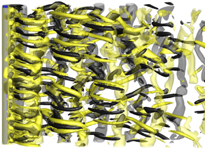
Instantaneous vorticity fields for AR = 0.125: (a) Re = 100 (mode A with vortex dislocations); (b) Re = 120 (ordered mode A); (c) Re = 170 (large-scale mode QP2); and (d) Re = 210 (small-scale structures). The translucent iso-surfaces represent spanwise vortices with |ω_z| = 1.0, while the opaque iso-surfaces represent streamwise vortices with |ω_x| = 0.5, 0.5, 0.7 and 1.5 for panels (a–d), respectively. Dark grey and light yellow denote positive and negative vorticity values, respectively. The flow is from left to right past the blue cylinder on the left.

Slightly prior to the re-stabilisation, the 3-D wake at Re = 120 is represented by ordered mode A structures (figure 19b) with periodic time evolution. This phenomenon is also confirmed by an additional case with a doubled L_z/D of 30, where six ordered spanwise periods of the mode A structures are observed. The regular and periodic mode A structures in the fully developed flow (without evolving into vortex dislocations) are not commonly observed in bluff-body flows. The reason for the suppression of vortex dislocation is that the strength of the mode A structures is limited (here by a gradual reduction of the strength of the mode A instability towards the re-stabilisation with increasing Re).

Beyond the 3-D mode A regime for Re = 81.5–122, the flow becomes 3-D again at Re ≥ 167.5 (figure 15a). For Re = 170, 180 and 200, the present 3-D DNS show that the wake is governed by the large-scale mode QP2 (figure 19c), which is consistent with the prediction by the Floquet analysis (figure 15). For Re ≥ 210, the wake is dominated by small-scale structures (figure 19d), which, according to the Floquet analysis results shown in figure 15, are mode A2 structures.

For AR = 0.125, the wake transition process predicted by the 3-D DNS is consistent with the sequence of wake instability modes predicted by the Floquet analysis (both following ‘mode A → 2-D → mode QP2 → mode A2’). This is because (i) although the development of the mode A structures may alter the pattern of the spanwise vorticity field, the alteration is ceased at the re-stabilisation to the 2-D flow and cannot influence subsequent 3-D modes (in contrast to the scenario of AR = 0.5 where mode A destabilises mode B), and (ii) unlike mode A, the mode QP2 structures do not alter the pattern of the spanwise vorticity field (i.e. the base flow) noticeably, such that both 3-D DNS and Floquet analysis predict the same subsequent mode A2. For example, figure 20(a) shows that the mode QP2 streamwise vortices develop in between of the spanwise vortices and thus induce minimal influence on the spanwise vortices. Therefore, the span-averaged spanwise vorticity field (figure 20b) is very similar to that predicted by the 2-D DNS (figure 20c).

Figure 20.

Vorticity fields for the case (AR, Re) = (0.125, 200): (a) an instantaneous streamwise vorticity (black and yellow for ω_x = ±1.5) and spanwise vorticity (red and blue for ω_z = ±1) field obtained from 3-D DNS; (b) the corresponding span-averaged spanwise vorticity field; and (c) an instantaneous spanwise vorticity field obtained from 2-D DNS. All vorticity fields are shown at the phase when the lift coefficient reaches a local maximum.

Quantitatively, owing to the slight interactions between the streamwise and spanwise vortices, and the nonlinear competition between the modes QP2 and A2, the critical Re for the wake transition from mode QP2 to mode A2 predicted by the 3-D DNS (Re = 200–210) is somewhat larger than that predicted by the Floquet analysis (Re = 174.7). A similar phenomenon is also observed for the case of a zero-thickness flat plate, where additional 3-D DNS performed in the present study identify the wake transition from mode QP2 to mode A2 at Re = 160–180, while the Floquet analysis by Choi & Yang (Reference Choi and Yang2014) predicted the mode A2 instability at a smaller Re of 139.1.

Figure 21 shows the St–Re, $\overline {{C_D}} - Re$ and ${C^{\prime}_L} - Re$ relationships for AR = 0.125. The 2-D results are reproduced from figure 7(d–f). For the 3-D results, the negligible deviations of the 3-D results from their 2-D counterparts at Re = 85 (close to the onset of the first three-dimensionality at Re = 81.5) suggests that the 3-D wake transition is supercritical, which is different from the subcritical mode A transition for AR = 0.5. The supercritical mode A transition for AR = 0.125 is confirmed by using the Landau equation for the case Re = 85. The supercritical nature of the 3-D transition suggests that, as Re > 81.5, the 3-D hydrodynamic forces gradually deviate from their 2-D counterparts (although due to limited data points, it looks as if there was a sudden drop at Re = 100). With the re-stabilisation over Re = 122–167.5, the hydrodynamic forces follow back the 2-D trend (with the 3-D symbols omitted for clarity). Beyond the onset of the second three-dimensionality, the 3-D results remain close to their 2-D counterparts over the mode QP2 regime of Re = 167.5–200, because the mode QP2 streamwise vortices are scarcely distributed along the spanwise direction (figure 19c) and also induce minimal influence on the spanwise vortices (figure 20). Because the two 2-D wake transitions still exist in the 3-D flow (figure 20a,b), the 3-D hydrodynamic forces largely follow the 2-D curve with both transitions. Subsequently, the 3-D results deviate significantly from their 2-D counterparts in the mode A2 regime of Re ≥ 210, because the mode A2 streamwise vortices are intensively developed in the immediate near wake of the cylinder (figure 19d), and the two 2-D wake transitions are significantly altered by the disordered mode A2 structures (figure 22 for Re = 210 versus figure 20 for Re = 200). In summary, the hydrodynamic forces for AR = 0.125 are governed by both 2-D and 3-D wake transitions (and their mutual influence, which also depends on the type of the 3-D mode).

Figure 21.

St–Re, $\overline {{C_D}} - Re$ and ${C^{\prime}_L} - Re$ relationships for AR = 0.125.

Figure 22.

Vorticity fields for the case (AR, Re) = (0.125, 210): (a) an instantaneous streamwise vorticity (black and yellow for ω_x = ±2) and spanwise vorticity (red and blue for ω_z = ±1.5) field obtained from 3-D DNS; (b) the corresponding span-averaged spanwise vorticity field; and (c) an instantaneous spanwise vorticity field obtained from 2-D DNS.