2.1. Reduced magnetohydrodynamics

Let $(M,g)$ be a compact, two-dimensional Riemannian manifold without boundary. The RMHD model on $(M,g)$ reads

(2.1) \begin{equation} \left \{ \begin{aligned} &\dot \omega =\left \{\omega ,\psi \right \}+\left \{\theta ,j\right \}\!, \quad &\omega =\Delta \psi , \\ &\dot \theta =\left \{\theta ,\psi \right \}\!, \quad &j=\Delta \theta , \end{aligned} \right . \end{equation}

where $\omega$ is the vorticity, $\psi$ is the stream function, $\theta$ is the magnetic potential, $j$ is the current density, all depending on time $t$ and $(x,y)\in M$ . The Laplace–Beltrami operator $\Delta$ is given in terms of the metric $g$ , and the Poisson bracket $\left \{\boldsymbol{\cdot },\boldsymbol{\cdot }\right \}$ is defined via the symplectic form (or area-form) $\varOmega$ on $M$ as

(2.2) \begin{equation} \left \{f,h\right \}=\varOmega (X_{f},X_{h}),\quad f,h\in C_{0}^{\infty }(M), \end{equation}

where $X_{f}$ , $X_{h}$ are Hamiltonian vector fields with Hamiltonian functions $f$ and $h$ respectively. Since $M$ is a compact manifold without a boundary, one can normalise all the fields $\omega ,j,\theta ,\psi$ to have zero-mean, i.e. they are elements of $C_{0}^{\infty }(M)$ .

The system (2.1) possesses a non-canonical Hamiltonian formulation in terms of a Lie–Poisson structure on the dual of a semidirect product Lie algebra. The Hamiltonian for (2.1) is

(2.3) \begin{equation} H=\frac {1}{2}\int \limits _{M}\left (|\boldsymbol{\nabla }\psi |^{2}+|\boldsymbol{\nabla }\theta |^{2} \right )\mathrm{d}x\mathrm{d}y = -\frac {1}{2}\int \limits _{M}(\omega \psi +\theta j)\mathrm{d}x\mathrm{d}y , \end{equation}

where the first term is the kinetic energy, and the second term is the magnetic energy. The Lie–Poisson bracket

(2.4) \begin{equation} \begin{split} [\![ F,G]\!]&=\int \limits _{M}\left [\omega \left \{\frac {\delta F}{\delta \omega },\frac {\delta G}{\delta \omega }\right \}+ \theta \left (\left \{\frac {\delta F}{\delta \theta },\frac {\delta G}{\delta \omega }\right \}+\left \{\frac {\delta F}{\delta \omega },\frac {\delta G}{\delta \theta }\right \}\right )\right ]\mathrm{d}x\mathrm{d}y \end{split} \end{equation}

is called the semidirect product bracket (Holm, Marsden & Ratiu Reference Holm, Marsden and Ratiu1998). The RMHD system (2.1) then reads

(2.5) \begin{equation} \dot F=[\![ F,H]\!], \end{equation}

where $F$ is an observable of the fields $\omega$ and $\theta$ .

System (2.1) has an infinite number of invariants parameterised by two arbitrary smooth functions $f\colon \mathbb{R}\to \mathbb{R}$ and $g\colon \mathbb{R}\to \mathbb{R}$

(2.6) \begin{equation} \mathcal{C}_{f}=\int \limits _{M}f(\theta )\mathrm{d}x\mathrm{d}y,\quad \mathcal{I}_{g}=\int \limits _{M}\omega g(\theta )\mathrm{d}x\mathrm{d}y. \end{equation}

These invariants are Casimirs, i.e. for any functional $\mathcal{J}(\omega ,\theta )$ , one has $[\![ \mathcal{C}_{f},\mathcal{J}]\!]=[\![ \mathcal{I}_{g},\mathcal{J}]\!]=0$ . We observe that $g(\theta )=\theta$ corresponds to the cross-helicity invariant, and $f(\theta )=\theta ^{2}$ corresponds to the mean-square magnetic potential, both critical in MHD turbulence. More generally, we refer to $\mathcal{C}_{f}$ as magnetic helicity and to $\mathcal{I}_{g}$ as cross-helicity. Of course, the Hamiltonian (2.3) is also conserved by the flow (2.1), but it is not a Casimir invariant. Instead, its conservation follows from the anti-symmetry of the Lie–Poisson bracket.

2.2. Hazeltine's model and the Charney--Hasegawa--Mima model

A three-field extension of the RMHD system (2.1) is given by the system of equations derived by Hazeltine (Reference Hazeltine1983)

(2.7) \begin{equation} \left \{ \begin{aligned} &\dot \omega =\left \{\omega ,\psi \right \}+\left \{\theta ,j\right \}\!, \\ &\dot \theta =\left \{\theta ,\psi \right \}-\alpha \left \{\theta ,\chi \right \}\!,\\ &\dot \chi =\left \{\chi ,\psi \right \}+\left \{\theta ,j\right \}, \end{aligned} \right . \end{equation}

where the new field $\chi$ represents the normalised deviation of the plasma density from a constant equilibrium value. The $\chi$ field is coupled to $\omega$ and $\theta$ via the length-scale parameter $\alpha \geqslant 0$ .

Particular cases of (2.7) include both low-beta limit of ideal RMHD and the CHM equation (Charney Reference Charney1948; Hasegawa & Mima Reference Hasegawa and Mima1977). First, the RMHD theory is recovered from (2.7) by setting $\alpha =0$ . Indeed, the system then decouples the $\omega$ and $\theta$ fields from the $\chi$ field, and the resulting equations constitute the RMHD system with the extra ‘passive’ field $\chi$ . Second, the CHM equation is obtained from (2.7) by presuming $\alpha \chi =\psi$ . In this case, $\dot \theta =0$ , and (2.7) simplifies to the equation

(2.8) \begin{equation} \frac {\partial }{\partial t}\left (\omega -\frac {\psi }{\alpha }\right )+\left \{\psi ,\omega \right \}=0,\quad \omega =\Delta \psi , \end{equation}

where $\psi (t,x,y)$ is the velocity streamfunction. Introducing the new field, potential vorticity, as $\sigma =\omega -\psi /\alpha$ , we get the transport equation for the field $\sigma$ related to the streamfunction $\psi$ via the homogeneous Helmholtz operator

(2.9) \begin{equation} \dot \sigma =\left \{\sigma ,\psi \right \}\!,\quad \sigma =\Delta \psi -\psi /\alpha. \end{equation}

The Casimir invariants for the system (2.9) are

(2.10) \begin{equation} \mathcal{C}_{f}=\int \limits _{M}f(\sigma )\mathrm{d}x\mathrm{d}y, \end{equation}

for arbitrary $f$ as before. The (2.9) also arises in geophysical fluid dynamics (Larichev & Reznik Reference Larichev and Reznik1976).

The Lie–Poisson bracket for Hazeltine’s (2.7) is (Hazeltine et al. Reference Hazeltine, Holm and Morrison1985; Holm Reference Holm1985)

(2.11) \begin{equation} \begin{split} [\![ F,G]\!]&=\int \limits _{M}\left [\omega \left \{\frac {\delta F}{\delta \omega },\frac {\delta G}{\delta \omega }\right \}+ \theta \left (\left \{\frac {\delta F}{\delta \theta },\frac {\delta G}{\delta \omega }\right \}+\left \{\frac {\delta F}{\delta \omega },\frac {\delta G}{\delta \theta }\right \}\right )\right .{}\\&\quad\left .+\, \chi \left (\left \{\frac {\delta F}{\delta \chi },\frac {\delta G}{\delta \omega }\right \}+\left \{\frac {\delta F}{\delta \omega },\frac {\delta G}{\delta \chi }\right \}\right )+ \chi \left \{\frac {\delta F}{\delta \chi },\frac {\delta G}{\delta \chi }\right \}\right .{}\\&\quad\left . +\, \theta \left (\left \{\frac {\delta F}{\delta \theta },\frac {\delta G}{\delta \chi }\right \}+\left \{\frac {\delta F}{\delta \chi },\frac {\delta G}{\delta \theta }\right \}\right )\right ]\mathrm{d}x\mathrm{d}y, \end{split} \end{equation}

and the Hamiltonian function is

(2.12) \begin{equation} H=-\frac {1}{2}\int \limits _{M}\left (\omega \psi +\theta j-\alpha \chi ^{2}\right )\!\mathrm{d}x\mathrm{d}y. \end{equation}

Thus, Hazeltine’s equations can be written

(2.13) \begin{equation} \dot F=[\![ F,H]\!], \end{equation}

for an observable $F$ of the fields $\omega$ , $\theta$ and $\chi$ . Furthermore, the corresponding Casimir invariants are

(2.14) \begin{equation} \mathcal{C}_{f}=\int \limits _{M}f(\theta )\mathrm{d}x\mathrm{d}y,\quad \mathcal{I}_{g}=\int \limits _{M}\chi g(\theta )\mathrm{d}x\mathrm{d}y,\quad \mathcal{P}_{k}=\int \limits _{M}k(\omega -\chi )\mathrm{d}x\mathrm{d}y, \end{equation}

for arbitrary smooth functions $f,g,k$ .

We observe that all the three models have different Casimir functions. In particular, the cross-helicity Casimir $\mathcal{I}_{g}$ in (2.6) is not preserved by (2.7), and (2.10) is not preserved by either of (2.7) and (2.1).

3.1. The RMHD--Zeitlin equations

The idea of finding a structure-preserving discretisation is based on quantisation theory, namely to replace the infinite-dimensional Poisson algebra of smooth functions $(C^{\infty }_{0}(S^{2}),\left \{\boldsymbol{\cdot },\boldsymbol{\cdot }\right \})$ with a finite-dimensional matrix approximation consisting of the Lie algebra of skew-Hermitian matrices $\mathfrak{su}(N)$ equipped with the scaled Lie bracket $[\boldsymbol{\cdot },\boldsymbol{\cdot }]_{N}= {1}/{\hbar }[\boldsymbol{\cdot },\boldsymbol{\cdot }]$ for $\hbar =2/\sqrt {N^{2}-1}$ . As $N\to \infty$ , the matrix Lie algebra $(\mathfrak{su}(N),[\boldsymbol{\cdot },\boldsymbol{\cdot }]_N)$ converges, via the spherical harmonics basis (see below), to the Poisson algebra $(C^{\infty }_{0}(S^{2}),\left \{\boldsymbol{\cdot },\boldsymbol{\cdot }\right \})$ of zero-mean smooth functions on $S^{2}$ (see, for example, the convergence result of Charles & Polterovich (Reference Charles and Polterovich2018)). A finite-dimensional approximation for the RMHD (2.1) is therefore given by the following RMHD–Zeitlin equations:

(3.1) \begin{equation} \left \{ \begin{aligned} &\dot W=\frac {1}{\hbar }[W,P]+\frac {1}{\hbar }[\varTheta ,J],\quad &W=\Delta _{N}P \\ &\dot \varTheta =\frac {1}{\hbar }[\varTheta ,P],\quad &J=\Delta _{N}\varTheta , \end{aligned} \right . \end{equation}

where $W,P,J,\varTheta \in \mathfrak{su}(N)$ are matrices and $\Delta _{N}\colon \mathfrak{su}(N)\to \mathfrak{su}(N)$ is the Hoppe–Yau Laplacian (Hoppe & Yau Reference Hoppe and Yau1998).

To obtain the connection between matrices, such as $W$ , and fields, such as $\omega$ , we consider the eigen-matrices of the Hoppe–Yau Laplacian $\Delta _N$ , which form a basis $T_{lm}^{N}$ , $l=0,1,\ldots , N-1,\,m=-l,\ldots ,l$ for $\mathfrak{su}(N)$ , called matrix harmonics. Then, for $W\in \mathfrak{su}(N)$ , one reconstructs the vorticity function $\omega \in C^{\infty }_{0}(S^{2})$ , up to the first $N^{2}$ terms of its Fourier decomposition in the spherical harmonics basis $Y_{lm}$ , by the correspondences $T_{lm}^{N} \sim Y_{lm}$ . For more details on mapping between the vorticity matrix $W\in \mathfrak{su}(N)$ and the vorticity function $\omega \in C^{\infty }_{0}(S^{2})$ , we refer to the publications by Modin & Viviani (Reference Modin and Viviani2024) and Modin & Roop (Reference Modin and Roop2025).

The system (3.1) constitutes a finite-dimensional Lie–Poisson flow on the dual $\mathfrak{f}^{*}$ of the semidirect product Lie algebra $\mathfrak{f}=\mathfrak{su}(N)\ltimes \mathfrak{su}(N)^{*}$ . The integral of a function on $S^2$ corresponds to $4\pi /N$ times the trace of the corresponding matrix. In particular, the Hamiltonian for (3.1) is obtained from the Hamiltonian (2.3) as

(3.2) \begin{equation} H(W,\varTheta )=\frac {2\pi }{N}\mathrm{tr}\big (W^{\dagger }P + \varTheta ^{\dagger }J \big ). \end{equation}

Likewise, the discretised Casimir invariants are

(3.3) \begin{equation} \mathcal{C}_{f}^{N}=\frac {4\pi }{N}\mathrm{tr}\left (f(\varTheta )\right )\!,\quad \mathcal{I}_{g}^{N}=\frac {4\pi }{N}\mathrm{tr}(Wg(\varTheta )). \end{equation}

As $N\to \infty$ , the Hamiltonian (3.2) and the Casimirs (3.3) converge to their continuous counterparts (2.3) and (2.6) (for $f$ and $g$ taken as monomials, see the paper by Modin & Roop (Reference Modin and Roop2025) for the exact result).

The matrix flow (3.1) is integrated in time using the Lie–Poisson-preserving time integrator $\varPhi _{h}\colon (W_{n},\varTheta _{n})\mapsto (W_{n+1},\varTheta _{n+1})$ defined by the equations

(3.4) \begin{equation} \begin{aligned} \varTheta _{n}&=\tilde \varTheta -\frac {\varepsilon }{2}[\tilde \varTheta ,\tilde {P}]-\frac {\varepsilon ^{2}}{4}\tilde {P}\tilde \varTheta \tilde {P}, \\ \varTheta _{n+1}&=\varTheta _{n}+\varepsilon [\tilde \varTheta ,\tilde {P}],\\ W_{n}&=\tilde W-\frac {\varepsilon }{2}[\tilde W,\tilde {P}]-\frac {\varepsilon }{2}[\tilde \varTheta ,\tilde J]-\frac {\varepsilon ^{2}}{4}(\tilde {P}\tilde {W}\tilde {P}+\tilde J\tilde \varTheta \tilde {P}+\tilde {P}\tilde \varTheta \tilde J ), \\ W_{n+1}&=W_{n}+\varepsilon [\tilde W,\tilde P]+\varepsilon [\tilde \varTheta ,\tilde J], \end{aligned} \end{equation}

where $\tilde P=\Delta _{N}^{-1}\tilde W$ , $\tilde J=\Delta _{N}\tilde \varTheta$ and $\varepsilon = \delta t/\hbar$ for the physical time step length $\delta t \gt 0$ . The integrator (3.4) exactlyFootnote ² preserves the Casimirs (3.3) for any choice of functions $f$ and $g$ , and nearly preserves the Hamiltonian (3.2), see Modin & Roop (Reference Modin and Roop2025).

The scheme (3.4) is implicitly defined, requiring root finding for the pair $(\tilde W,\tilde \varTheta )$ as an intermediate step. This is achieved by fixed point iterations. Given the state $(W_{n},\varTheta _{n})$ , the midpoint variables $(\tilde W,\tilde \varTheta )$ are found from the first and the third equation in (3.4), and then used to get the updated state $(W_{n+1},\varTheta _{n+1})$ by means of the second and the fourth equations in (3.4). Preservation of Casimirs by the method (3.4) is guaranteed provided that the midpoint state $(\tilde W,\tilde \varTheta )$ is found exactly. In practice, the state $(\tilde W,\tilde \varTheta )$ is found up to the tolerance of the fixed point algorithm, and therefore the Casimirs are preserved at least up to that tolerance. In the forthcoming simulations, the tolerance of the fixed point iterations is $10^{-13}$ .

Contrary to generic Lie–Poisson integrators, the method (3.4) is free of matrix exponentials and therefore scales efficiently as the matrix size grows. The complexity per time step is $O(N^{3})$ , see Cifani et al. (Reference Cifani, Viviani and Modin2023).

3.2. The Hazeltine--Zeitlin and CHM--Zeitlin equations

Before we write the corresponding discretisation for Hazeltine’s model (2.7), let us note that it is convenient to introduce a new field $q=\omega -\chi$ . Then the system (2.7) becomes

(3.5) \begin{equation} \left \{ \begin{aligned} &\dot q=\left \{q,\psi \right \}, \\ &\dot \theta =\left \{\theta ,\psi -\alpha \chi \right \},\\ &\dot \chi =\left \{\chi ,\psi \right \}+\left \{\theta ,j\right \}, \end{aligned} \right . \end{equation}

and the corresponding semidirect product Lie–Poisson bracket for (3.5) in terms of the new fields $q,\theta ,\chi$ simplifies to

(3.6) \begin{equation} \begin{split} [\![ F,G]\!]&=\int \limits _{M}\left [\chi \!\left \{\frac {\delta F}{\delta \chi },\frac {\delta G}{\delta \chi }\right \}+ \theta \!\left (\left \{\frac {\delta F}{\delta \theta },\frac {\delta G}{\delta \chi }\right \}+\left \{\frac {\delta F}{\delta \chi },\frac {\delta G}{\delta \theta }\right \}\right )+q\!\left \{\frac {\delta F}{\delta q},\frac {\delta G}{\delta q}\right \}\right ]\mathrm{d}x\mathrm{d}y. \end{split} \end{equation}

The Hazeltine–Zeitlin equations for (3.5) are then

(3.7) \begin{equation} \left \{ \begin{aligned} &\dot Q=\frac {1}{\hbar }[Q,P], \\ &\dot \varTheta =\frac {1}{\hbar }[\varTheta ,P-\alpha R],\\ &\dot R=\frac {1}{\hbar }[R,P]+\frac {1}{\hbar }[\varTheta ,J], \end{aligned} \right . \end{equation}

where $R\in \mathfrak{su}(N)$ is the matrix for the field $\chi$ .

The introduction of the new field $q$ reveals the underlying Lie algebra for the matrix system (3.7). Indeed, the first equation, for the $Q$ matrix, is isospectral, and the last two equations for matrices $\varTheta$ and $R$ constitute the Lie–Poisson flow on the dual of the semidirect product Lie algebra, similar to (3.1), and all the three equations are coupled through the Hamiltonian function. Summarising, the flow (3.7) is a Lie–Poisson system on the dual $\mathfrak{f}^{*}$ of the Lie algebra

(3.8) \begin{align} \mathfrak{f}=\mathfrak{su}(N)\oplus (\mathfrak{su}(N)\ltimes \mathfrak{su}(N)^{*}), \end{align}

with the Casimir invariants

(3.9) \begin{equation} \mathcal{C}_{f}^{N}=\frac {4\pi }{N}\mathrm{tr}\left (f(\varTheta )\right )\!,\quad \mathcal{I}_{g}^{N}=\frac {4\pi }{N}\mathrm{tr}(Rg(\varTheta )),\quad \mathcal{P}_{h}^{N}=\frac {4\pi }{N}\mathrm{tr}(k(Q)), \end{equation}

for arbitrary smooth functions $f,g,k$ , and the Hamiltonian

(3.10) \begin{equation} H=\frac {2\pi }{N}\mathrm{tr} (W^{\dagger }P+\varTheta ^{\dagger } J-\alpha R^{\dagger }R). \end{equation}

A Lie–Poisson time integrator for (3.7) is obtained by combining the isospectral integrator for the matrix $Q$ , and the magnetic midpoint integrator for the matrices $R$ and $\varTheta$ , which gives the scheme

(3.11) \begin{equation} \begin{aligned} &\varTheta _{n}=\tilde \varTheta -\frac {\varepsilon }{2}[\tilde \varTheta ,\tilde {M}]-\frac {\varepsilon ^{2}}{4}\tilde {M}\tilde \varTheta \tilde {M}, \\ &\varTheta _{n+1}=\varTheta _{n}+\varepsilon [\tilde \varTheta ,\tilde {M}],\\ &Q_{n}=\tilde {Q}-\frac {\varepsilon }{2}[\tilde {Q},\tilde {P}]-\frac {\varepsilon ^{2}}{4}\tilde {P}\tilde {Q}\tilde {P}, \\ &Q_{n+1}=Q_{n}+\varepsilon [\tilde {Q},\tilde {P}],\\ &R_{n}=\tilde {R}-\frac {\varepsilon }{2}[\tilde {R},\tilde {M}]-\frac {\varepsilon }{2}[\tilde \varTheta ,\tilde {J}]-\frac {\varepsilon ^{2}}{4}(\tilde {M}\tilde {R}\tilde {M}+\tilde {J}\tilde \varTheta \tilde {M}+\tilde {M}\tilde \varTheta \tilde {J}),\\ &R_{n+1}=R_{n}+\varepsilon [\tilde {R},\tilde {M}]+\varepsilon [\tilde \varTheta ,\tilde {J}], \end{aligned} \end{equation}

where $\tilde {M}=\tilde {P}-\alpha \tilde {R}$ and with $\varepsilon =\delta t/\hbar$ as before. Similar to the integrator (3.4), the scheme (3.11) preserves the Casimirs (3.9) and nearly preserves the Hamiltonian (3.10).

Finally, we present the CHM–Zeitlin equation for the matrix discretisation of CHM equations (2.9), namely

(3.12) \begin{equation} \dot \varSigma =\frac {1}{\hbar }[\varSigma ,P],\quad \varSigma =\Delta _{N}P- P/\alpha . \end{equation}

The Casimir invariants and the Hamiltonian for (3.12) are given by

(3.13) \begin{equation} \mathcal{C}_{f}^{N}=\frac {4\pi }{N}\mathrm{tr}(f(\varSigma )),\quad H(\varSigma )=\frac {2\pi }{N}\mathrm{tr}(\varSigma ^{\dagger }P). \end{equation}

In this case, Lie–Poisson time integration is obtained via the isospectral midpoint method (Modin & Viviani, Reference Modin and Viviani2020b )

(3.14) \begin{equation} \varSigma _{n}=\tilde \varSigma -\frac {\varepsilon }{2}\bigl[\tilde \varSigma ,\tilde {P}\bigr]-\frac {\varepsilon ^{2}}{4}\tilde {P}\tilde \varTheta \tilde {P},\quad \varSigma _{n+1}=\tilde \varSigma +\varepsilon \bigl[\tilde \varSigma ,\tilde {P}\bigr],\quad \tilde \varSigma =\Delta _{N}\tilde {P}-\tilde {P}/\alpha . \end{equation}

4.1. Reduced magnetohydrodynamics

The simulation results for RMHD are obtained by using the method (3.4). In all the simulations, the matrix dimension is $N=512$ , and the initial condition is prepared such that the fields contain $(l_{\max}+1)^{2}$ terms in the spherical harmonics basis, with $l_{\max}=10$ and with each coefficient randomly generated from the normal distribution. One can observe that the Hamiltonian (3.2) splits into two parts: the kinetic part $(2\pi /N)\mathrm{tr}(W^{\dagger }P)$ produced by the vorticity dynamics, and the magnetic part $(2\pi /N)\mathrm{tr}(\varTheta ^{\dagger }J)$ produced by the magnetic potential dynamics. We generate the initial conditions in such a way that kinetic and magnetic energy terms initially contribute approximately equally to the total energy $H(W,\varTheta )$ . The final time for the simulations is $T=559$ .

For non-magnetic fluids, hydrodynamical turbulence, which in the ideal setting is modelled by the vorticity transport equation, is known to be fundamentally different in two and three dimensions. In particular, two-dimensional (2-D) hydrodynamical turbulence is characterised by the inverse energy cascade, in contrast to 3-D turbulence which has a forward energy cascade. In RMHD, the addition of the Lorentz force to the vorticity advection equation leads to rapid amplification of the vorticity via the formation of vortex filaments. This cannot happen in 2-D turbulence, where the vorticity function is advected, so its values cannot change. From the point of view of analysis, the situation for RMHD is more similar to the 3-D Euler equations than to the 2-D Euler equations. Indeed, the RMHD (2.1) are similar in structure to the axisymmetric 3-D Euler equations (Modin & Preston Reference Modin and Preston2025), which exhibit finite-time blow-up of vorticity. On the other hand, the equilibrium spectra obtained by Fyfe & Montgomery (Reference Fyfe and Montgomery1976) suggest an inverse cascade of the mean-square magnetic potential. This inverse cascade of the mean-square magnetic potential is believed to be a mechanism leading to the formation of large magnetic eddies.

Let us now see if and how these phenomena are manifested in our simulations.

In our study, we divide the dynamics into a ‘smooth’ or ‘slow’ part, represented by the fields $\psi$ and $\theta$ , and ‘rough’ or ‘fast’ part, represented by the fields $\omega$ and $j$ . For the slow part, the evolution of the streamfunction $\psi$ and the magnetic potential $\theta$ is shown in figure 2. We observe the formation of a magnetic dipole consisting of positive and negative blobs obtained through intermediate mixing. The streamfunction $\psi (t)$ becomes grainy in its long-time behaviour, with no sign of formation of large-scale structures, albeit traces of the large-scale structure in $\theta (t)$ are visible. In particular, vortex formations (i.e. localised swirling) for $\psi (t)$ and $\theta (t)$ are observed approximately at the same locations.

Figure 2.

RMHD: evolution of the velocity streamfunction $\psi (t)$ (left) and the magnetic potential $\theta (t)$ (right). The magnetic potential $\theta$ develops into the dipole configuration through intermediate mixing. The streamfunction $\psi$ does not develop large-scale structures, but one can observe circulations at locations of the magnetic eddies.

Figure 3.

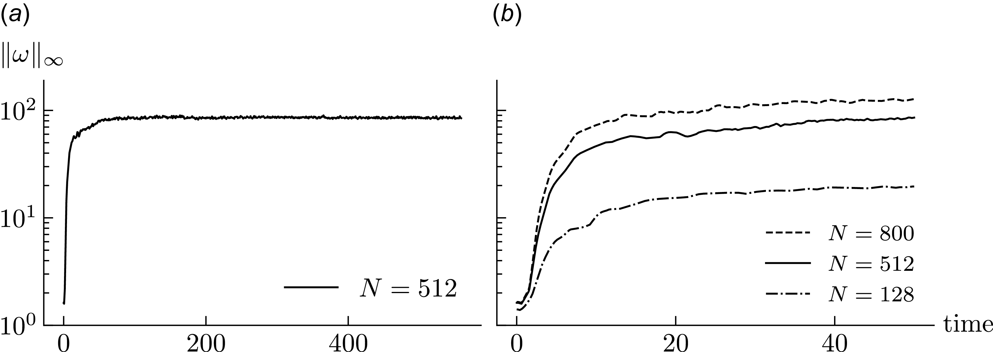
RMHD: evolution of the vorticity field supremum norm $\lVert \omega \rVert _\infty$ . (a) For a simulation with spatial resolution $N=512$ , the value initially grows rapidly and then reach a plateau at approximately $t=100$ . (b) For simulations with the same initial data, the plateau is larger in magnitude for higher spatial resolution. This indicates that the value grows indefinitely as $N\to \infty$ .

For the fast part, the evolution of the fields $\omega (t)$ and $j(t)$ is shown in figure 4. We see the formation of filaments in both $\omega$ and $j$ . These are well resolved only for a short while, up until approximately $t=2$ . After that, they are too narrow and too entangled to be resolved. At the final time $t=559$ , we obtained a noisy result with large vorticity values. One should interpret this noise as the truncation of an extremely delicate filament structure. Notice in figure 3(a) that the supremum norm of $\omega$ rapidly grows from approximately $2$ to approximately $100$ (the current density field $j$ shadows $\omega$ , with rapid growth from approximately $2$ to approximately $100$ ). These values settle at larger magnitudes if a higher spatial resolution is used, which is shown in figure 3(b), where we present the evolution of the supremum norm of the vorticity field $\omega$ for resolutions $N=128$ , $N=512$ and $N=800$ . This behaviour is similar to the axisymmetric 3-D Euler equations, where numerical simulations via matrix hydrodynamics also show growth of the supremum norm of vorticity for growing spatial resolution (Modin & Preston Reference Modin and Preston2025). As mentioned, the axisymmetric 3-D Euler equations are known to have solutions that lead to blow-up of the vorticity in finite time. Whether the RMHD equations exhibit finite time blow-up is an open mathematical analysis problem.

Figure 4.

RMHD: evolution of the vorticity $\omega (t)$ (left) and the current density $j(t)$ (right). Vorticity and current density islands resemble each other. Both fields $\omega$ and $j$ are significantly amplified, which makes the dynamics resolved only for relatively short times.

In figure 5, we demonstrate the evolution of the total energy, as well as its kinetic $E_{kin}$ and magnetic $E_{magn}$ components. While the total energy is conserved, its kinetic and magnetic parts redistribute in such a way that magnetic energy initially grows in time, reaches its maximum and then decays while dominating over the kinetic energy. Kinetic energy has the opposite dynamics. In the long term, there is a tendency of equipartition between kinetic and magnetic energies.

Figure 5.

RMHD: (a) total energy variation, and (b) kinetic $E_{kin}$ and magnetic $E_{magn}$ energy evolution over time. The total energy $E_{magn} + E_{kin}$ is conserved up to a relative error of approximately $10^{-5}$ . The magnetic and kinetic energy components are redistributed with a tendency towards equipartition.

Figure 6.

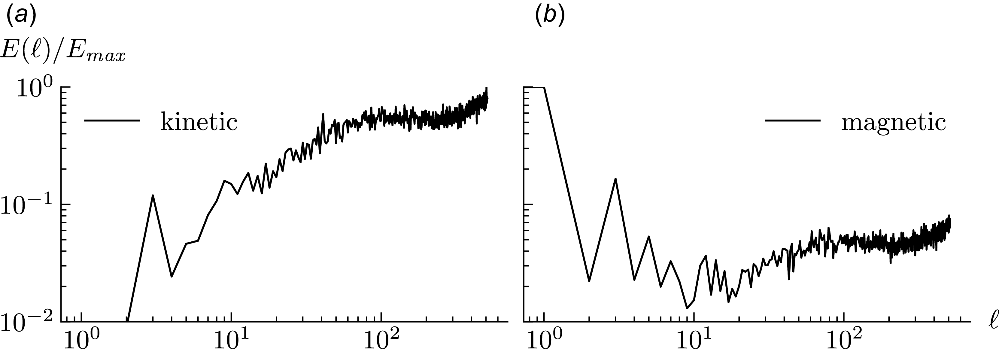
RMHD: kinetic (a) and magnetic (b) energy spectra at the final time $t=559$ . A major part of the kinetic energy is concentrated at high frequencies, indicating a forward kinetic energy cascade. The magnetic energy is mostly concentrated at lower frequencies and thereafter homogeneously distributed over the higher frequencies, indicating a backward cascade of magnetic energy; the effect is further emphasised in the spectrum of the mean-square magnetic potential, shown in figure 7.

Figure 7.

RMHD: mean square of magnetic potential $A$ spectrum at (a) initial time $t=0$ , and (b) final time $t=559$ . An inverse cascade of $A$ is observed with the approximate scaling $\ell ^{-1.9}$ .

The normalised spectra for magnetic and kinetic energies at the final time $t=559$ are presented in figure 6. As predicted by the statistical theory, the kinetic energy experiences a direct cascade, as most of it is concentrated in the modes of high $l$ . The magnetic energy, on the contrary, is localised at lower frequencies, which is reflected by larger magnitudes in its spectrum at low frequencies. This also reflects simulations in figure 2, showing the formation of the large-scale magnetic dipole. Both kinetic and magnetic energies are uniformly distributed over higher frequencies, as seen in figure 6.

Finally, we present the spectrum for the mean-square magnetic potential $A=\int _{S^{2}}\theta ^{2}\mathrm{d}x\mathrm{d}y$ in figure 7, which clearly indicates its inverse cascade with the slope approximately $-2$ .

4.2. The Charney--Hasegawa--Mima model

For the CHM model simulation, the length-scale parameter is chosen to be $\alpha =1/2$ . In figure 8, we present the evolutions of the potential vorticity field $\sigma (t)$ . The spatial resolution parameter $N=512$ , and the final simulation time is $t=76$ , by which the system reaches a statistically equilibrium configuration consisting of two positive and two negative vortex blobs in a quasi-periodic motion. We observe the formation of the four vortex condensates regardless of the value of the total angular momentum, contrary to the Euler equations, where the four vortex blob configuration is reached from initial states having trivial total angular momentum. The mixing phase of merging small vortices of the same sign into larger vortices continues until the time approximately $t=10.5$ , when the four-blob configuration is reached. After that, no further mixing occurs.

Figure 8.

The CHM model: evolution of the potential vorticity field $\sigma (t)$ . Smooth randomly generated initial distribution evolves into four vortex blob configuration (two positive and two negative) involved in a quasi-periodic motion.

The kinetic energy spectrum is shown in figure 9, which indicates the presence of the inverse cascade with the broken line shape of the slope.

Figure 9.

The CHM model: kinetic energy spectrum of the final state at $t=76$ . The spectrum has a broken line shape with the scaling $l^{-3}$ for the low-frequency part, and $l^{-1.3}$ for the high-frequency part.

4.3. Hazeltine's model

For the Hazeltine model simulation, we choose the length-scale parameter $\alpha =1/2$ , and prepare the initial vorticity distribution $\omega _{0}$ with vanishing total angular momentum. The motivation for such a choice comes from the long-time simulations of the incompressible Euler equations, where the dynamics settles at the four-blob configuration in the case of vanishing total angular momentum; see, e.g. Modin & Viviani (Reference Modin and Viviani2020a ), where it is conjectured that vorticity mixing continues until the system reaches nearly integrable behaviour and remains close to it in the sense of the Kolmogorov-Arnold-Moser theory. As in the previous simulations of the RMHD system, we choose initial condition with equal contribution to the total energy from all the fields. The spatial resolution is again $N=512$ and the total simulation time is set to $t=562$ .

Figure 10.

Hazeltine: evolution of the vorticity $\omega (t)$ field. Smooth randomly generated initial vorticity distribution evolves into vortex blob configuration on the small-scale background noise.

As seen in figure 10, the vorticity dynamics in the Hazeltine model is significantly different from that of RMHD. Indeed, the vorticity evolution resembles that of the 2-D Euler. Namely, one observes the formation of four large-scale vortex blobs, two positive and two negative, through intermediate mixing. Notice, in particular, that the vorticity values are almost conserved, which is unexpected since $\omega$ is not transported in Hazeltine’s model. The $\chi$ field seems to compensate the amplification of the vorticity $\omega$ taking place in RMHD dynamics. On the other hand, the blob formation is different from that in the Euler dynamics and the CHM dynamics. Indeed, the blobs travel ‘in dipole pairs’, where the vorticity dipole is formed by a negative and a positive vortex blob without, however, further mixing. In the Euler dynamics, on the contrary, blobs of different sign tend to repel each other. This behaviour indicates that the extension of RMHD by the density variation field $\chi$ makes the plasma turbulence more alike to the 2-D hydrodynamical turbulence.

Indeed, we underline that the vorticity field dynamics in Hazeltine’s model has a clear scale separation, which is absent in the long-time RMHD dynamics for the same space resolution: large-scale vortex blobs slowly travel on the small scale rapidly evolving background. This is also seen from the kinetic energy spectrum in figure 11. The low-frequency part of the spectrum, which corresponds to large spatial scales, has the slope $l^{-3}$ , and the high-frequency part corresponding to small spatial scales behaves as $l^{-1.3}$ . The slopes are in agreement with the spectral properties of the Euler flows, see Modin & Viviani (Reference Modin and Viviani2022), where one observes a similar scale separation with the slopes $l^{-1}$ for small scales and $l^{-3}$ for large scales.

Figure 11.

Hazeltine: kinetic energy spectrum of the final state at $t=562$ . The spectrum has a broken line shape with the scaling $l^{-3}$ for the low-frequency part, and $l^{-1.3}$ for the high-frequency part.

Analogously to the simulation in figure 2 for the RMHD model, we present the corresponding evolution of the fields $\theta (t)$ and $\psi (t)$ for the Hazeltine model in figure 12. The qualitative dynamics of the magnetic potential $\theta (t)$ in the Hazeltine model is similar to that in RMHD, although it is transported by a different field. One can see from figure 12 formation of the magnetic dipole through intermediate mixing.

Figure 12.

Hazeltine: evolution of the velocity streamfunction $\psi (t)$ (left) and the magnetic potential $\theta (t)$ (right). The magnetic potential $\theta$ develops into the dipole configuration through intermediate mixing. The streamfunction $\psi$ develops large-scale structures resembling those in the vorticity $\omega$ dynamics.

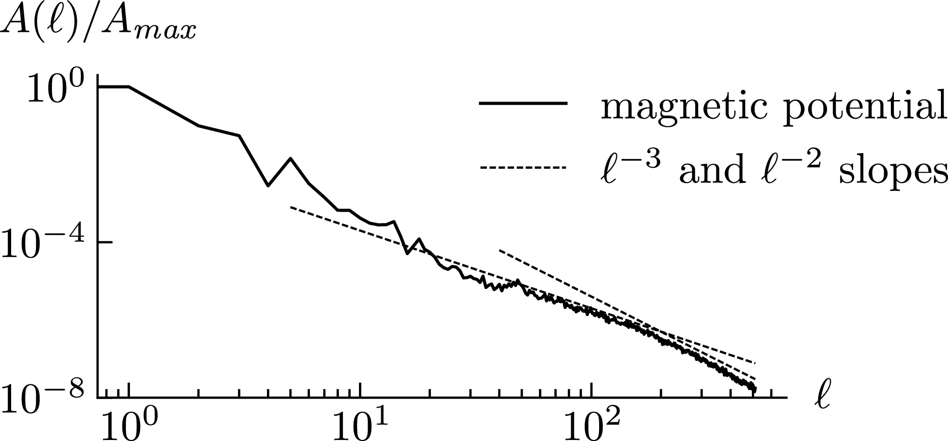
The spectral properties of the mean-square magnetic potential are different from those in the RMHD model. Figure 13 shows that the scaling for $A$ is $l^{-3}$ , with an interval of frequencies $20\lesssim l \lesssim 100$ where the scaling is $l^{-2}$ . This still indicates the inverse cascade of the mean-square magnetic potential, which reflects the formation of large-scale magnetic eddies shown in figure 12.

Figure 13.

Hazeltine: mean-square magnetic potential spectrum of the final state at $t=562$ . The observed inverse cascade is consistent with the build-up of the magnetic dipole seen in figure 12.

We conclude this section with the dynamics of the density variation field $\chi (t)$ . Although the $\chi (t)$ field fulfils the same equation as the field $\omega (t)$ in the RMHD model, one does not observe a vast amplification of $\chi (t)$ in the Hazeltine model, as seen from figure 14. In the long-time dynamics, one observes circulations centred approximately at locations of the magnetic potential eddies.

Figure 14.

Hazeltine: evolution of the density variation field $\chi (t)$ . There are no clear large-scale structures remaining at large times, although we observe some circulating filament-like structures centred about the locations of magnetic blobs in figure 12.