


1 Introduction
The purpose of this paper is the analysis of geometric properties of the solutions of a toy model of a quasi-static droplet motion with contact angle hysteresis effects.
Capillary surfaces incident to a solid surface are often subject to a phenomenon known as contact angle hysteresis. Instead of a single stable contact angle determined by the material properties, as predicted by the classical Young’s law, there is a pinning interval, or range of stable apparent contact angles. Thus, under small forcings, the contact line can “stick” in a similar way to classical static friction in mechanics. The origin of contact angle hysteresis and the appropriate modeling of its effects remain the subject of much interest in the physics, engineering, and mathematics literature [Reference Mohammad Karim25].
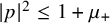
In the present model, we consider a droplet on a flat d-dimensional plane whose free surface is given as a graph of a function $u = u(t, x)$
,
$u = u(t, x)$
, $u: [0, \infty ) \times U \to [0, \infty )$
, where
$u: [0, \infty ) \times U \to [0, \infty )$
, where $U \subset \mathbb {R}^d$
is a connected domain with compact complement; see Figure 1. The sets
$U \subset \mathbb {R}^d$
is a connected domain with compact complement; see Figure 1. The sets $\Omega (u(t)) := \{u(t)> 0\}$
and
$\Omega (u(t)) := \{u(t)> 0\}$
and $\{u(t) = 0\}$
are respectively the wet and dry regions at time t. At the domain boundary
$\{u(t) = 0\}$
are respectively the wet and dry regions at time t. At the domain boundary $\partial U$
, the height of the droplet surface is a given function of time
$\partial U$
, the height of the droplet surface is a given function of time $F = F(t)$
. We assume that the time scale at which the droplet reaches equilibrium is much shorter than the time scale at which F changes, that is, the evolution is quasi-static. Therefore at each time
$F = F(t)$
. We assume that the time scale at which the droplet reaches equilibrium is much shorter than the time scale at which F changes, that is, the evolution is quasi-static. Therefore at each time $u(t)$
minimizes the linearized surface area of the graph
$u(t)$
minimizes the linearized surface area of the graph $\{(x, u(t, x)): u(t, x)> 0\}$
, and at the boundary of the wet region
$\{(x, u(t, x)): u(t, x)> 0\}$
, and at the boundary of the wet region $\partial \{u(t)> 0\} \cap U$
the contact slope is within the allowed interval
$\partial \{u(t)> 0\} \cap U$
the contact slope is within the allowed interval $|\nabla u(t)|^2 \in [1 - \mu _-, 1 + \mu _+]$
with some
$|\nabla u(t)|^2 \in [1 - \mu _-, 1 + \mu _+]$
with some $\mu _- \in (0,1)$
and
$\mu _- \in (0,1)$
and $\mu _+> 0$
. In summary, at each time
$\mu _+> 0$
. In summary, at each time $t \in [0, T]$
,
$t \in [0, T]$
, $u(t)$
is a solution of the local stability condition
$u(t)$
is a solution of the local stability condition
 $$ \begin{align} \begin{cases} \Delta u(t)= 0 & \text{ in } \ \Omega(u(t))\cap U,\\ 1-\mu_- \leq |\nabla u(t)|^2 \leq 1+\mu_+ & \text{on } \partial \Omega(u(t)) \cap U, \end{cases} \end{align} $$
while it satisfies the Dirichlet boundary condition
 $$ \begin{align*} u(t) = F(t) \qquad \text{on } \partial U. \end{align*} $$
Side view (left) and the top view (right) of the setup for the one-phase free boundary problem.

It remains to specify how the droplet reacts to the changes in the boundary condition $F(t)$
. Here it seems reasonable to require that the support
$F(t)$
. Here it seems reasonable to require that the support $\Omega (u(t)) = \{u(t)> 0\}$
adjusts as little as necessary so that the conditions in (1.1) can be satisfied. This should mean that it expands (resp. shrinks) only at points where the contact angle condition
$\Omega (u(t)) = \{u(t)> 0\}$
adjusts as little as necessary so that the conditions in (1.1) can be satisfied. This should mean that it expands (resp. shrinks) only at points where the contact angle condition $|\nabla u|^2 \leq 1 + \mu _+$
(resp.
$|\nabla u|^2 \leq 1 + \mu _+$
(resp. $|\nabla u|^2 \geq 1 - \mu _-$
) saturates. This heuristic “motion law” suggests the dynamic slope condition
$|\nabla u|^2 \geq 1 - \mu _-$
) saturates. This heuristic “motion law” suggests the dynamic slope condition
 $$ \begin{align} |\nabla u(t)|^2(x) = 1\pm \mu_\pm \quad \text{ if } \quad \pm V_n(\Omega(u(t)),x)>0 \quad \text{on } \ \partial \Omega(u(t)) \cap U, \end{align} $$
where $V_n(\Omega (u(t)),x)$
is the outward normal velocity of
$V_n(\Omega (u(t)),x)$
is the outward normal velocity of $\Omega (u(t))$
at
$\Omega (u(t))$
at $x \in \partial \Omega (u(t))$
.
$x \in \partial \Omega (u(t))$
.
It is natural to frame this as an obstacle problem for $u(t)$
as long as the forcing F is piecewise monotone. More precisely, we assume that there is a finite set Z such that
$u(t)$
as long as the forcing F is piecewise monotone. More precisely, we assume that there is a finite set Z such that
 $$ \begin{align} F: [0,T] \to (0,\infty) \text{ is Lipschitz and changes monotonicity only on } Z. \end{align} $$
The above motivates the following definition.
Definition 1.1. We say that $u: [0, T] \times \overline U \to [0, \infty )$
is an obstacle solution (O) in U driven by F on
$u: [0, T] \times \overline U \to [0, \infty )$
is an obstacle solution (O) in U driven by F on $\partial U$
if
$\partial U$
if
-
1. (Initial data) $u(0)$
is a viscosity solution of the local stability conditions (1.1).
$u(0)$
is a viscosity solution of the local stability conditions (1.1). -
2. (Dirichlet forcing) For all
$t \in [0,T]$
(1.4)
$$ \begin{align} u(t) = F(t) \ \text{ on } \ \partial U. \end{align} $$
-
3. (Obstacle condition) For every
$(s,t) \cap Z = \emptyset $
, so that F is monotone on
$[s,t]$
,
$u(t)$
is the minimal supersolution of (1.1) and (1.4) above
$u(s)$
when F is increasing on
$[s,t]$
(resp. maximal subsolution below
$u(s)$
when F is decreasing).


The notions of minimal supersolution and maximal subsolution above are in the viscosity solutions/Perron’s method sense; see Section 4 for more details. The stability condition on the initial data is for convenience, otherwise the solution could jump at the initial time resulting in a “replacement” initial data satisfying (1.1).
It is not hard to show that an obstacle solution satisfies the local stability and dynamic slope conditions. However, the question whether the conditions (1.1) and (1.2) uniquely characterize the obstacle solution is less obvious and we give an affirmative answer in the strongly star-shaped setting (Definition 4.9) with additional regularity assumptions. In fact, we do not expect this to be the case when there are jumps in the evolution, which cannot be easily ruled out in the non-star-shaped setting.
Theorem 1.2 (see Theorem 4.10)
Let F satisfy (1.3), and let u be an obstacle solution in the sense of Definition 1.1 and let $\Omega _0 := \Omega (u(0))$
:
$\Omega _0 := \Omega (u(0))$
:
-
(i) If u is uniformly nondegenerate at its free boundary (which holds if
$d=2$
or if
$\Omega _0$
is strongly star-shaped, see Lemma A.2), then u satisfies the local stability condition (1.1) and the dynamic slope condition (1.2) in the viscosity solutions sense; Definition 4.3 and Definition 4.8. -
(ii) Furthermore, if
$\Omega _0$
is a strongly star-shaped
$C^{1,\alpha }$
domain, then any viscosity solution of (1.1) and (1.2) is the unique obstacle solution.


In a general setting, the obstacle solution (O) can jump in time due to topological changes of the wet region $\Omega (u(t))$
; see Section 2 for examples. The handling of jumps seems physically reasonable as, in a certain sense, the solution jumps “as late as possible”. We believe that this is an important feature of this notion. This is in a contrast to an alternative approach to modeling the quasi-static evolution: a rate-independent evolution of the Bernoulli functional
$\Omega (u(t))$
; see Section 2 for examples. The handling of jumps seems physically reasonable as, in a certain sense, the solution jumps “as late as possible”. We believe that this is an important feature of this notion. This is in a contrast to an alternative approach to modeling the quasi-static evolution: a rate-independent evolution of the Bernoulli functional
 $$ \begin{align} \mathcal{J}(v) = \int_U |\nabla v|^2 + \mathbf{1}_{\{v>0\}} \ dx, \qquad v \in H^1(U), \end{align} $$
where $\mathbf {1}_{\{v> 0\}}$
is the indicator function of the set
$\mathbf {1}_{\{v> 0\}}$
is the indicator function of the set $\Omega (v) := \{v>0\}$
, with a dissipation distance
$\Omega (v) := \{v>0\}$
, with a dissipation distance
 $$\begin{align*}\operatorname{Diss}(v_1,v_2) := \mu_+|\Omega(v_1) \setminus \Omega(v_0)| + \mu_-|\Omega(v_0) \setminus \Omega(v_1)|,\end{align*}$$
again driven by the Dirichlet forcing F.
The authors explored this approach in a companion paper [Reference Feldman, Kim and Požár17] so we refer the reader to that paper for details. Here we briefly review the important definitions. The approach is inspired by the work of DeSimone, Grunewald, and Otto [Reference DeSimone, Grunewald and Otto15], with theory developed by Alberti and DeSimone [Reference Alberti and DeSimone1]. Those works considered the surface energy capillarity functional with volume forcing using the energetic framework of rate-independent systems [Reference Mielke and Tomáš24].
In [Reference Feldman, Kim and Požár17] the following notion of a solution was introduced:
Definition 1.3. A measurable $u : [0,T] \to H^1(U)$
is an energy solution (E) of the quasi-static evolution problem driven by Dirichlet forcing F if the following hold:
$u : [0,T] \to H^1(U)$
is an energy solution (E) of the quasi-static evolution problem driven by Dirichlet forcing F if the following hold:
-
1. (Forcing) For all
$t \in [0,T]$
$$\begin{align*}u(t) = F(t) \ \text{ on } \partial U\end{align*}$$
-
2. (Global stability) The solution
$u(t)\in H^1(U)$
and satisfies for all
$t \in [0,T]$
: (1.6)
$$ \begin{align} \mathcal{J}(u(t)) \leq \mathcal{J}(u') + \operatorname{Diss}(u(t),u') \qquad \text{for all }u' \in u(t)+ H^1_0(U). \end{align} $$
-
3. (Energy dissipation inequality) For every
$0 \leq t_0 \leq t_1 \leq T$
it holds (1.7)Here
$$ \begin{align} \mathcal{J}(u({t_0}))-\mathcal{J}(u({t_1})) + \int_{t_0}^{t_1}2 \dot{F}(t)P(t) \ dt \geq \operatorname{Diss}(u(t_0),u(t_1)). \end{align} $$
$P(t) = P(u(t))= \int _{\partial U} \frac {\partial u(t)}{\partial n} \ dS$
is an associated pressure.


A formal first variation of the global stability condition (1.6) shows that $u(t)$
should indeed be a solution of (1.1). However, due to the global nature of the stability condition, the solution can in principle jump to a more favorable energy configuration earlier than would be physically reasonable; see Section 2.2 for a discussion of an example. Therefore we do not expect that the obstacle solutions (O) and energy solutions (E) coincide when jumps occur.
$u(t)$
should indeed be a solution of (1.1). However, due to the global nature of the stability condition, the solution can in principle jump to a more favorable energy configuration earlier than would be physically reasonable; see Section 2.2 for a discussion of an example. Therefore we do not expect that the obstacle solutions (O) and energy solutions (E) coincide when jumps occur.
The authors showed in [Reference Feldman, Kim and Požár17] that the limit points as timestep $\delta \to 0$
of the following minimizing movements scheme are energy solutions. Define a piecewise constant interpolation
$\delta \to 0$
of the following minimizing movements scheme are energy solutions. Define a piecewise constant interpolation
 $$ \begin{align} u_{\delta}(t):= u_{\delta}^k \ \text{ and } \ F_\delta(t) = F(k\delta) \ \text{ if } \ t\in [k\delta, (k+1)\delta). \end{align} $$
of the time-discrete scheme
 $$ \begin{align} u_{\delta}^k \in {\text{argmin}} \left\{ \mathcal{J}(w) + \operatorname{Diss}(u^{k-1}_\delta, w): w\in F(k\delta)+ H^1_0(U)\right\}. \end{align} $$
Plots of boundaries of obstacle solution (O) simulations. Solid curves represent $\partial \Omega (t) \cap U$
plotted for evenly spaced values of
$\partial \Omega (t) \cap U$
plotted for evenly spaced values of $F(t)$
, with the initial shape dashed.
$F(t)$
, with the initial shape dashed. $\partial U$
is given by a dotted curve. Top left: Disconnected annuli initial data, jump discontinuity on touching. Top right: Receding situation (decreasing
$\partial U$
is given by a dotted curve. Top left: Disconnected annuli initial data, jump discontinuity on touching. Top right: Receding situation (decreasing $F(t)$
) with initial data given by the last step of the top left image. Note that the jump occurs at a different configuration, as late as possible. Bottom left: Different radius annuli, free boundary peels from the larger annulus after the jump. Bottom right: Stadium type initial data, convexity is not preserved.
$F(t)$
) with initial data given by the last step of the top left image. Note that the jump occurs at a different configuration, as late as possible. Bottom left: Different radius annuli, free boundary peels from the larger annulus after the jump. Bottom right: Stadium type initial data, convexity is not preserved.

As our second main result, we show that the obstacle solutions coincide with the notion of energy solutions that is generated from the minimizing scheme in the case of strongly star-shaped data. As we will see, convexity is not preserved in the problem, Section 2.3, and thus star-shapedness is a natural setting for this problem where no topology change or jump occurs in the evolution, allowing for pointwise regularity analysis.
Theorem 1.4 (see Theorem 4.10 and Theorem 5.4)
Let F satisfy (1.3), and let $u(0)$
be strongly star-shaped (Definition 4.9) with bounded support
$u(0)$
be strongly star-shaped (Definition 4.9) with bounded support $\mathbb {R}^d \setminus U \subset \Omega _0$
. Further assume that
$\mathbb {R}^d \setminus U \subset \Omega _0$
. Further assume that $\partial \Omega _0$
is
$\partial \Omega _0$
is $C^{1,\alpha }$
and
$C^{1,\alpha }$
and $u(0)$
satisfies (1.1). Then the following holds for u, the unique obstacle solution (O) on
$u(0)$
satisfies (1.1). Then the following holds for u, the unique obstacle solution (O) on $[0,T]$
with initial data
$[0,T]$
with initial data $u(0)$
:
$u(0)$
:
-
(i) The unique (O) solution u is also the unique energy solution that is the limit of the minimizing movement scheme with initial data
$u(0)$
. Moreover the solutions (1.8) of the discrete-time minimizing scheme converge uniformly to
$u(t)$
with a uniform rate that only depends on F,
$\mu _{\pm }$
. -
(ii)
$u(t)$
is strongly star-shaped for each time. -
(iii) u and the boundary of
$\kern1.2pt\Omega := \{u>0\}$
are
$C^{0,1}_tC_x \cap L^\infty _tC^{1,\min \{\frac {1}{2},\alpha \}-}_x$
.


Philosophically, (a) indicates that the local stability and dynamic slope conditions contain all the information in (E) or (O) except for the jump law. We expect that the spatial regularity $C^{1,\frac {1}{2}}_x$
described in (iii) is optimal. Specifically, when the contact line “peels” or “de-laminates” from the initial data, as shown in Figure 2, free boundary
$C^{1,\frac {1}{2}}_x$
described in (iii) is optimal. Specifically, when the contact line “peels” or “de-laminates” from the initial data, as shown in Figure 2, free boundary $\partial \Omega (u(t))$
looks like a solution of a thin-obstacle / Signorini problem near its thin free boundary. See Section 3, specifically Theorem 3.5 and (3.8), for a more precise description of this asymptotic expansion. It is well known that Signorini solutions with smooth obstacle may peel away from their thin free boundary with as little as
$\partial \Omega (u(t))$
looks like a solution of a thin-obstacle / Signorini problem near its thin free boundary. See Section 3, specifically Theorem 3.5 and (3.8), for a more precise description of this asymptotic expansion. It is well known that Signorini solutions with smooth obstacle may peel away from their thin free boundary with as little as $C^{1,\frac {1}{2}}_x$
regularity due to the model solution
$C^{1,\frac {1}{2}}_x$
regularity due to the model solution $\text {Re}((x+iy)^{3/2})$
, see the survey [Reference Fernández-Real18] for details and references. Although we do not fully explore the sharp asymptotic expansion of the free boundary near a de-lamination point
$\text {Re}((x+iy)^{3/2})$
, see the survey [Reference Fernández-Real18] for details and references. Although we do not fully explore the sharp asymptotic expansion of the free boundary near a de-lamination point $x_0 \in \partial \Omega (u(t))$
, we do establish the (almost) optimal upper growth bound
$x_0 \in \partial \Omega (u(t))$
, we do establish the (almost) optimal upper growth bound $|x-x_0|^{1+\min \{1/2, \alpha \}-}$
.
$|x-x_0|^{1+\min \{1/2, \alpha \}-}$
.
Besides the regularity theory developed in Section 3, the novel comparison principle for viscosity solutions of (1.1) and (1.2), Proposition 4.20, also plays a central role in this theorem. The convergence result for minimizing movements solutions part (i) follows a similar idea to Chambolle’s proof of convergence of the Almgren-Taylor-Wang / Luckhaus-Sturzenhecker schemes for mean curvature flow [Reference Chambolle11, Reference Almgren, Taylor and Wang2, Reference Luckhaus and Sturzenhecker22].
The star-shapedness is a key hypothesis in Theorem 1.4. Perhaps most importantly, the star-shaped geometry is used to ensure that there is no jump in the obstacle solution (O). This is crucial to obtain part (i), since the energy solutions and obstacle solutions have different jump laws, as we illustrate by an example in Section 2.
The local cone monotonicity implied by star-shapedness is also used to obtain the regularity result in (iii). Cone monotonicity allows us to show, in Section 3, that all blow-ups at the free boundary are half-plane solutions. Then we can invoke the “flat means smooth” results of [Reference Chang-Lara and Savin12, Reference Ferreri and Velichkov19] for Bernoulli obstacle problems.
It is difficult to derive geometric properties of the evolution purely from the energetic structure. At the time of the original appearance of this manuscript we were not aware of any purely energetic method to obtain higher regularity of the free boundary. Even seemingly simple properties seemed difficult to prove just from energetics; for example, it was not clear whether arbitrary energy solutions (E) must respect time monotonicity of the Dirichlet forcing. After the original appearance of this work, Collins and the first author [Reference Collins and Feldman13] have partially resolved these questions in the context of minimizing movements solutions.
1.1 Open questions
An important motivation for introducing the obstacle solutions, even outside of the star-shaped case, is that it handles time jump discontinuities well. This is in contrast to the global energetic solutions studied in [Reference Alberti and DeSimone1, Reference Feldman, Kim and Požár17] which jump as early as is energetically favorable. Instead, the obstacle solution jumps “as late and as little as possible”. This is regarded as a more physically accurate jump condition, similar to the notion of balanced viscosity solutions: see, for example, [Reference Mielke, Rossi and Savaré23] or [Reference Mielke and Tomáš24, Chapter 3.8.2]. The obstacle solution dissipates the “right” amount of energy on its jumps, but does not obviously yield an energetic notion of jump dissipation. It would be interesting to study the possible connection of the balanced viscosity notion with our obstacle solution (O).
It would be interesting to study the regularity of obstacle solutions outside of the star-shaped setting. Unlike the energy solutions considered in [Reference Collins and Feldman13], obstacle solutions certainly develop singularities even in low dimensions. For example, when two components touch and then merge after advancing one expects at least one singular point with the “two-plane” blow-up profile $(1+\mu _+)|x_d|_+$
. This does not occur for energy solutions since the jump discontinuity occurs before the components touch. We expect similar kinds of topological changes are possible even when the initial data has connected positivity set, so it really seems important to understand the two-plane singular points in order to extend our results beyond the star-shaped setting. Unfortunately the main tool in the general regularity theory, the Weiss monotonicity formula [Reference Weiss30], applies to variational solutions. It is not clear if obstacle minimal supersolutions / maximal subsolutions satisfy the Weiss monotonicity formula.
$(1+\mu _+)|x_d|_+$
. This does not occur for energy solutions since the jump discontinuity occurs before the components touch. We expect similar kinds of topological changes are possible even when the initial data has connected positivity set, so it really seems important to understand the two-plane singular points in order to extend our results beyond the star-shaped setting. Unfortunately the main tool in the general regularity theory, the Weiss monotonicity formula [Reference Weiss30], applies to variational solutions. It is not clear if obstacle minimal supersolutions / maximal subsolutions satisfy the Weiss monotonicity formula.
1.2 Notations and conventions
We list several notations and conventions which will be in force through the paper.
-
▹ We call a constant universal if it only depends on d and
$\mu _+>0$
,
$\mu _- \in (0,1)$
. -
▹ We will refer to universal constants by
$C \geq 1$
and
$0<c \leq 1$
and allow such constants to change from line to line of the computation. -
▹ We often abuse notation and write
$\Omega (t)$
instead of
$\Omega (u(t))$
etc. -
▹
$u^*$
and
$u_*$
denote the upper-semicontinuous envelope and the lower-semicontinuous envelope of u, respectively, see (4.2). We write USC and LSC respectively as shorthand for upper semicontinuous and lower semicontinuous. -
▹
$F + H^1_0(U)$
refers to the space of functions in
$H^1(U)$
with trace F on
$\partial U$
.


2 Motivating examples
In order to introduce the problem and motivate the phenomena we will study in the paper we present several examples with analytical computations and numerical simulations.
2.1 Numerical simulations
The obstacle solutions (O) can be relatively easily approximated by a large time limit ( $\tau \to \infty $
) of a dynamic contact angle problem: Suppose that F is increasing on
$\tau \to \infty $
) of a dynamic contact angle problem: Suppose that F is increasing on $[s, t]$
. Given
$[s, t]$
. Given $u(s)$
,
$u(s)$
, $u(t)$
can be found as the limit
$u(t)$
can be found as the limit $\tau \to \infty $
of the unique, monotone solution of the free boundary problem
$\tau \to \infty $
of the unique, monotone solution of the free boundary problem
 $$ \begin{align*} \left\{\begin{aligned} - \Delta w(\tau) &= 0, &&\text{in } \{w(\tau)> 0\} \cap U,\\ V_n &= \max(|\nabla w| - (1 + \mu_+)^{1/2}, 0) && \text{on } \partial\{w(\tau) > 0\} \cap U,\\ w(\tau) &= F(t), && \text{on } \partial U,\\ \{w(0) > 0\} &= \{u(s) > 0\}. \end{aligned}\right. \end{align*} $$
Analogously, for F decreasing on $[s, t]$
we replace the velocity law by
$[s, t]$
we replace the velocity law by $V_n = \min (|\nabla w| - (1 - \mu _-)^{1/2}, 0)$
.
$V_n = \min (|\nabla w| - (1 - \mu _-)^{1/2}, 0)$
.
A numerical solution can be found by adapting the level set method introduced in [Reference Gibou, Fedkiw, Cheng and Kang20], stopping at $\tau $
when
$\tau $
when $|V_n| < \varepsilon $
for some small parameter
$|V_n| < \varepsilon $
for some small parameter $\varepsilon> 0$
. Plots in Figure 2 were produced this way.
$\varepsilon> 0$
. Plots in Figure 2 were produced this way.
2.2 Jump conditions for (global) energetic vs obstacle solutions
Next we consider an example where the jump time for the energy solutions is different from the jump time for the obstacle evolution. Heuristically speaking the obstacle evolution solutions jump as late and as little as possible, while the (global) energy solutions jump whenever it becomes energetically favorable.
Consider a domain U which is the complement of two disjoint closed disks and initial data given by two disjoint annuli. Then under increasing $F(t)$
the solution will consist of two disjoint annuli until the value of the forcing when the boundaries of the two annuli meet at a single point. As F continues increasing past that critical value the solution will need to jump outwards to a new state. This situation is depicted in the simulations in Figure 2.
$F(t)$
the solution will consist of two disjoint annuli until the value of the forcing when the boundaries of the two annuli meet at a single point. As F continues increasing past that critical value the solution will need to jump outwards to a new state. This situation is depicted in the simulations in Figure 2.
The energy solution with the same data and forcing must jump before the value of the forcing when the two annuli touch. One way to see this is that the blow-up at the touching point of the annuli is a two plane solution of the form
 $$\begin{align*}v(x) = (1+\mu_+)^{1/2} |x \cdot e|.\end{align*}$$
However this blow-up does not satisfy the global stability condition in (E), since the harmonic replacement in any open region has the same positivity set but lower Dirichlet energy. Since any blow-up of a globally stable state is also globally stable we conclude that no energy solution can coincide with the obstacle solution all the way to the jump time.
2.3 Convexity is not preserved under the obstacle evolution
Consider the Bernoulli free boundary problem in the complement of a convex obstacle K
 $$\begin{align*}- \Delta u = 0 \ \text{ in } \ \{u>0\} \setminus K, \ \text{ with } \ |\nabla u| =1 \ \text{ on } \ \partial \{u>0\} \setminus K. \end{align*}$$
It is known, see Henrot and Shahgholian [Reference Henrot and Shahgholian21], that the (unique) compactly supported solution of this problem has convex super-level sets. In particular if one considers the obstacle solution (O) without pinning $\mu _\pm = 0$
, then the solution
$\mu _\pm = 0$
, then the solution $u(t)$
of the obstacle evolution (which depends only on the current value
$u(t)$
of the obstacle evolution (which depends only on the current value $F(t)$
due to the lack of hysteresis) is convex at all times.
$F(t)$
due to the lack of hysteresis) is convex at all times.
It is natural to ask whether convexity is still preserved under (O) in the case of nontrivial pinning interval $\mu _\pm>0$
. In fact it is not. We give a simulation of a counterexample in Figure 2 and present a sketched proof here.
$\mu _\pm>0$
. In fact it is not. We give a simulation of a counterexample in Figure 2 and present a sketched proof here.
Consider the case of $K = B_1$
,
$K = B_1$
, $F(0) = 1$
, and an initial region
$F(0) = 1$
, and an initial region $\Omega _0$
which is a “stadium” type initial data which is a large portion of the strip
$\Omega _0$
which is a “stadium” type initial data which is a large portion of the strip $-a < x_2 < a$
capped off by two circles of radius a centered at
$-a < x_2 < a$
capped off by two circles of radius a centered at $(\pm b,0)$
. Here
$(\pm b,0)$
. Here $0 < a-1 \ll 1$
and
$0 < a-1 \ll 1$
and $b \gg 1$
. The initial region
$b \gg 1$
. The initial region $\Omega _0$
and K uniquely determine the initial profile
$\Omega _0$
and K uniquely determine the initial profile $u_0$
, which does have convex super-level sets due to [Reference Caffarelli and Spruck10]. Fix the pinning interval by the relations
$u_0$
, which does have convex super-level sets due to [Reference Caffarelli and Spruck10]. Fix the pinning interval by the relations
 $$\begin{align*}\mu_+ := \max_{\partial \Omega_0} (|\nabla u_0|^2-1) \ \text{ and } \ \mu_-:=\max_{\partial \Omega_0} (1 - |\nabla u_0|^2). \end{align*}$$
By symmetry considerations the first maximum is achieved at $(0,\pm a)$
and the second at
$(0,\pm a)$
and the second at $(\pm (b+a),0)$
. We can guarantee that both maxima are positive by choosing the a close to
$(\pm (b+a),0)$
. We can guarantee that both maxima are positive by choosing the a close to $1$
and b large. Now increasing
$1$
and b large. Now increasing $F(t)$
slightly above
$F(t)$
slightly above $1$
the free boundary needs to immediately move outwards near
$1$
the free boundary needs to immediately move outwards near $(0,\pm a)$
since the slope there is already saturated at
$(0,\pm a)$
since the slope there is already saturated at $|\nabla u_0(0,a)|^2 = 1+\mu _+$
, but since this is exactly the maximum value of the slope the outwards movement will only be in a small neighborhood of those two points. This motion must produce nonconvexity because the domain
$|\nabla u_0(0,a)|^2 = 1+\mu _+$
, but since this is exactly the maximum value of the slope the outwards movement will only be in a small neighborhood of those two points. This motion must produce nonconvexity because the domain $\Omega (t)$
will have outward normal
$\Omega (t)$
will have outward normal $e_2$
both at some point
$e_2$
both at some point $(0,a+\delta (t))$
and at
$(0,a+\delta (t))$
and at $(b,a)$
.
$(b,a)$
.
This argument could be justified rigorously using Theorem 1.4.
3 Regularity theory of Bernoulli obstacle problems
In this section we consider a pair of obstacle problems for the Bernoulli free boundary problem, one with an obstacle from above and the other with an obstacle from below. The two problems are similar but not exactly symmetric, as we will see below in the analysis. The regularity theory of the problem with obstacle from above has been developed by Chang-Lara and Savin [Reference Chang-Lara and Savin12], and as we were finishing preparing this paper their theory has been extended to the obstacle from below case by Ferreri and Velichkov [Reference Ferreri and Velichkov19]. We present the problems, recall the flat implies smooth regularity results from the above-mentioned works, and then show how to achieve the initial flatness and full regularity under a cone monotonicity hypothesis which is appropriate for our work.
3.1 Bernoulli obstacle problems
Let U be an open region, the domain. We say that u is a solution / supersolution / subsolution of the (unconstrained) Bernoulli free boundary problem in U if
 $$ \begin{align} \begin{cases} \Delta u = 0 &\text{in } \{u>0\} \cap U,\\ |\nabla u| = 1 &\text{on } \ \partial \{u>0\} \cap U. \end{cases} \end{align} $$
Let the obstacle O be another open region with $C^{1,\alpha }$
boundary.
$C^{1,\alpha }$
boundary.
Definition 3.1. A function $u \in C(\overline {U})$
is a solution of the Bernoulli problem in U with obstacle O from below if
$u \in C(\overline {U})$
is a solution of the Bernoulli problem in U with obstacle O from below if
 $$ \begin{align} \begin{cases} \Delta u = 0 &\text{in } \{u>0\} \cap U\\ u>0 &\text{in } O \cap U \\ |\nabla u| = 1 &\text{on } \ (\partial \{u>0\} \setminus \overline{O}) \\ |\nabla u| \leq 1 &\text{on } \Lambda:=\ (\partial\{u>0\} \cap \partial O). \end{cases} \end{align} $$
Definition 3.2. A function $u \in C(\overline {U})$
is a solution of the Bernoulli problem in U with obstacle O from above if
$u \in C(\overline {U})$
is a solution of the Bernoulli problem in U with obstacle O from above if
 $$ \begin{align} \begin{cases} \Delta u = 0 &\text{in } \{u>0\} \cap U\\ u=0 &\text{in } \ \overline{U} \setminus O\\ |\nabla u| = 1&\text{on } \ (\partial \{u>0\} \cap O) \\ |\nabla u| \geq 1 &\text{on } \Lambda:= \ (\partial\{u>0\} \cap \partial O). \end{cases} \end{align} $$
See Figure 3 for depictions of obstacle solutions. The PDEs are solved in the standard viscosity sense; see, for example, [Reference Chang-Lara and Savin12] or Definition A.3 below.
Left: Obstacle from above, slope is larger than $1$
everywhere and saturates where free boundary bends into O. Right: Obstacle from below, slope is smaller than
$1$
everywhere and saturates where free boundary bends into O. Right: Obstacle from below, slope is smaller than $1$
everywhere and saturates where free boundary bends away from
$1$
everywhere and saturates where free boundary bends away from $\overline {O}$

3.2 Additional hypotheses
The obstacle below (resp. above) problems do not provide any a-priori bound on the slope at the free boundary from below (resp. above). Given a regular domain O and a specific boundary data on $\partial U$
one could establish such bounds on the interior. However it is more convenient for us to just list these additional bounds as hypotheses which will be in force for some (but not all) of the statements below. Let
$\partial U$
one could establish such bounds on the interior. However it is more convenient for us to just list these additional bounds as hypotheses which will be in force for some (but not all) of the statements below. Let $0 < \kappa < 1$
and consider the hypothesis: in the obstacle from below case
$0 < \kappa < 1$
and consider the hypothesis: in the obstacle from below case
 $$ \begin{align} |\nabla u| \geq \kappa \ \text{ in the viscosity sense on } \ \partial \{u>0\} \cap U, \end{align} $$
and in the obstacle from above case
 $$ \begin{align} |\nabla u| \leq \kappa^{-1} \ \text{ in the viscosity sense on } \ \partial \{u>0\} \cap U. \end{align} $$
3.3 Existence and typical examples
An indicative example of u solving a Bernoulli problem with obstacle from below (3.2) is the Perron’s method obstacle minimal supersolution
 $$ \begin{align} u(x) := \inf\{v(x): v \text{ is a supersolution of (3.1)}, v = g \text{ on } \partial U, \text{ and } v>0 \text{ in } O \cap \overline{U}\}. \end{align} $$
Here $g \in C(\partial U)$
is some boundary condition. In order for the minimal supersolution to also be positive on O we need to put some additional condition on g. Notice that every supersolution in (3.6) is above w, the solution of the Dirichlet problem
$g \in C(\partial U)$
is some boundary condition. In order for the minimal supersolution to also be positive on O we need to put some additional condition on g. Notice that every supersolution in (3.6) is above w, the solution of the Dirichlet problem
 $$\begin{align*}\Delta w = 0 \ \text{ in } \ O \cap U, \ w = 0 \ \text{ on } \ \partial O \cap U, \ \text{ and } \ w = g \ \text{ on }\ \partial U \cap \overline{O}. \end{align*}$$
So if $w>0$
in O then u will be positive in O as well. In particular it would suffice to assume that
$w>0$
in O then u will be positive in O as well. In particular it would suffice to assume that
 $$\begin{align*}g> 0 \ \text{ on } \ O \cap \partial U.\end{align*}$$
The obstacle solution property follows from the typical Perron’s method arguments. Local upward perturbations are possible everywhere in U, so u is a supersolution everywhere, while local downward perturbations are possible only away from $\partial \{u>0\} \cap \overline {O}$
limiting the subsolution property.
$\partial \{u>0\} \cap \overline {O}$
limiting the subsolution property.
An indicative example of u solving a Bernoulli problem with obstacle from above (3.3) is the obstacle maximal subsolution
 $$ \begin{align} u(x) := \sup\{v(x): v \text{ a subsolution of (3.1) in } U, v = g \text{ on } \partial U, \text{ and } \{v>0\} \subset O\}. \end{align} $$
For consistency the positivity set of g on $\partial U$
should be contained in
$\partial U$
should be contained in $O \cap \partial U$
. As before Perron’s method applies, arbitrary downward perturbations are possible so u is a subsolution everywhere, but local upward perturbations are only allowed away from
$O \cap \partial U$
. As before Perron’s method applies, arbitrary downward perturbations are possible so u is a subsolution everywhere, but local upward perturbations are only allowed away from $\partial \{u>0\} \cap \overline {O}$
.
$\partial \{u>0\} \cap \overline {O}$
.
Remark 3.3. As in [Reference Chang-Lara and Savin12] it is also possible to construct solutions to (3.3) by minimal supersolution Perron’s method, or by energy minimization. However, it is the maximal subsolutions that we will encounter in this work. This is something we need to be careful with, since nondegeneracy at the free boundary is a more delicate issue for maximal subsolutions.
3.4 Flat implies
$C^{1,\frac {1}{2}-}$
and regularity of cone monotone solutions

First let us recall the flat implies $C^{1,1-}$
regularity away from the obstacle. This result is originally due to Caffarelli [Reference Caffarelli8, Reference Caffarelli9]. A more recent alternative proof by De Silva [Reference De Silva14] has motivated the techniques used to study the obstacle problems we are considering.
$C^{1,1-}$
regularity away from the obstacle. This result is originally due to Caffarelli [Reference Caffarelli8, Reference Caffarelli9]. A more recent alternative proof by De Silva [Reference De Silva14] has motivated the techniques used to study the obstacle problems we are considering.
Theorem 3.4 (Flat implies
$C^{1,1-}$
for unconstrained Bernoulli [Reference Caffarelli8, Reference Caffarelli9])

Let u solve (3.1) in $B_1$
and
$B_1$
and $0 \in \partial \{u>0\}$
. For any
$0 \in \partial \{u>0\}$
. For any $\beta \in (0,1)$
there is
$\beta \in (0,1)$
there is $\varepsilon _0>0$
and
$\varepsilon _0>0$
and $C \geq 1$
universal so that if
$C \geq 1$
universal so that if
 $$\begin{align*}(x \cdot e - \varepsilon)_+ \leq u(x) \leq (x\cdot e + \varepsilon)_+ \ \text{ in } \ B_1\end{align*}$$
for some $\varepsilon \leq \varepsilon _0$
, then for all
$\varepsilon \leq \varepsilon _0$
, then for all $0 < r < 1$
and some
$0 < r < 1$
and some $|\nabla u(0)| = 1$
 $$\begin{align*}(x \cdot \nabla u(0) - C\varepsilon r^{1+\beta})_+ \leq u(x) \leq (x\cdot \nabla u(0) + C\varepsilon r^{1+\beta})_+ \ \text{ in } \ B_r.\end{align*}$$
Next we recall a similar flat implies smooth result on the contact set between the solution and the obstacle. Consider the contact set of the free boundary with the obstacle $\Lambda := \partial \{u>0\} \cap \partial O$
. Let us denote
$\Lambda := \partial \{u>0\} \cap \partial O$
. Let us denote $\partial '\Lambda $
to be the boundary of
$\partial '\Lambda $
to be the boundary of $\Lambda $
relative to
$\Lambda $
relative to $\partial O$
.
$\partial O$
.
Theorem 3.5 (Flat implies
$C^{1,\frac {1}{2}-}$
at the contact set [Reference Chang-Lara and Savin12, Reference Ferreri and Velichkov19])

Let u solve either (3.3) or (3.2) in $B_1$
and
$B_1$
and $0 \in \partial ' \Lambda $
, O be a
$0 \in \partial ' \Lambda $
, O be a $C^{1,\alpha }$
obstacle, and e be the inward normal to O at
$C^{1,\alpha }$
obstacle, and e be the inward normal to O at $0$
. For any
$0$
. For any $0 < \beta < \min \{\alpha ,\frac {1}{2}\}$
there is
$0 < \beta < \min \{\alpha ,\frac {1}{2}\}$
there is $\varepsilon _0>0$
and
$\varepsilon _0>0$
and $C \geq 1$
universal so that if
$C \geq 1$
universal so that if
 $$\begin{align*}(x \cdot e - \varepsilon)_+ \leq u(x) \leq (x\cdot e + \varepsilon)_+ \ \text{ in } \ B_1\end{align*}$$
for some $\varepsilon \leq \varepsilon _0$
, then for all
$\varepsilon \leq \varepsilon _0$
, then for all $0 < r < 1$
 $$\begin{align*}(x \cdot e - C\varepsilon r^{1+\beta})_+ \leq u(x) \leq (x\cdot e + C\varepsilon r^{1+\beta})_+ \ \text{ in } \ B_r.\end{align*}$$
In both the obstacle above and obstacle below cases the proof is based on establishing an asymptotic expansion for flat solutions of the form
 $$ \begin{align} u(x) = (x \cdot e + \varepsilon w(x) + o(\varepsilon))_+ \end{align} $$
where w is a solution of a certain Signorini or thin obstacle problem and $\varepsilon $
is the flatness in
$\varepsilon $
is the flatness in $B_1$
as in the hypothesis of Theorem 3.5. The
$B_1$
as in the hypothesis of Theorem 3.5. The $C^{1,\frac {1}{2}}$
optimal regularity for the Signorini problem is the reason for the
$C^{1,\frac {1}{2}}$
optimal regularity for the Signorini problem is the reason for the $C^{1,\frac {1}{2}-}$
regularity which appears here, and is likely (almost) optimal. The idea of the argument, which is based on a compactness principle using a special Harnack inequality for flat solutions, goes back to the work of De Silva [Reference De Silva14].
$C^{1,\frac {1}{2}-}$
regularity which appears here, and is likely (almost) optimal. The idea of the argument, which is based on a compactness principle using a special Harnack inequality for flat solutions, goes back to the work of De Silva [Reference De Silva14].
It is important for us to obtain a full regularity result without the flatness assumption. Of course some assumption is still necessary, singular solutions exist in higher dimensions, and fitting with the strongly star-shaped geometry we study later in the paper we will consider obstacle solutions satisfying a cone monotonicity condition. For the statement define
 $$ \begin{align} \text{Cone}(e, \theta):= \{e': e'\cdot e \geq 1-\theta\} \ \text{ for } \ e \in S^{d-1} \ \text{ and } \ \theta \in (0,1). \end{align} $$
Theorem 3.6. Suppose O is a bounded set with $C^{1,\alpha }$
boundary, and that u solves either (3.3) and (3.5) or (3.2) and (3.4) in
$C^{1,\alpha }$
boundary, and that u solves either (3.3) and (3.5) or (3.2) and (3.4) in $B_1$
. Assume also that there are
$B_1$
. Assume also that there are $e \in S^{d-1}$
and
$e \in S^{d-1}$
and $1\geq c_0>0$
so that u is monotone increasing in the directions of the cone
$1\geq c_0>0$
so that u is monotone increasing in the directions of the cone $\text {Cone}(e, c_0)$
.
$\text {Cone}(e, c_0)$
.
Then for any $0 < \beta < \min \{\alpha ,\frac {1}{2}\}$
the positivity set
$0 < \beta < \min \{\alpha ,\frac {1}{2}\}$
the positivity set $\{u>0\}$
is a
$\{u>0\}$
is a $C^{1,\beta }$
domain in
$C^{1,\beta }$
domain in $B_{1/2}$
and
$B_{1/2}$
and $u\in C^{1,\beta }(\overline {\{u>0\}} \cap B_{1/2})$
. The
$u\in C^{1,\beta }(\overline {\{u>0\}} \cap B_{1/2})$
. The $C^{1,\beta }$
norms depend only on
$C^{1,\beta }$
norms depend only on $\alpha $
,
$\alpha $
, $\kappa $
,
$\kappa $
, $c_0$
, d, and the
$c_0$
, d, and the $C^{1,\alpha }$
norm of
$C^{1,\alpha }$
norm of $\partial O$
.
$\partial O$
.
Remark 3.7. Chang-Lara and Savin [Reference Chang-Lara and Savin12] prove the optimal $C^{1,\frac {1}{2}}$
regularity in the case when the obstacle is
$C^{1,\frac {1}{2}}$
regularity in the case when the obstacle is $C^{1,\alpha }$
regular for some
$C^{1,\alpha }$
regular for some $1/2 < \alpha \leq 1$
. This matches the regularity of the thin obstacle/Signorini problem, which appears as the first order term in the asymptotic expansion for
$1/2 < \alpha \leq 1$
. This matches the regularity of the thin obstacle/Signorini problem, which appears as the first order term in the asymptotic expansion for $\varepsilon $
-flat solutions in the flatness parameter
$\varepsilon $
-flat solutions in the flatness parameter $\varepsilon $
. Since our obstacles are generated from the evolution itself and therefore have at most
$\varepsilon $
. Since our obstacles are generated from the evolution itself and therefore have at most $C^{1,\frac {1}{2}}$
regularity after the first monotonicity change, obtaining the optimal regularity is more delicate in our problem. As shown in [Reference Rüland and Shi27] there can be logarithmic losses of regularity at this critical scaling. To avoid getting into these technical details we aim to establish the (almost) optimal regularity
$C^{1,\frac {1}{2}}$
regularity after the first monotonicity change, obtaining the optimal regularity is more delicate in our problem. As shown in [Reference Rüland and Shi27] there can be logarithmic losses of regularity at this critical scaling. To avoid getting into these technical details we aim to establish the (almost) optimal regularity $C^{1,\frac {1}{2}-}$
. As we did not carefully track the logarithmic factors, and the cited example in [Reference Rüland and Shi27] concerns a problem with specifically designed x-dependent coefficients, a sharper result might be available.
$C^{1,\frac {1}{2}-}$
. As we did not carefully track the logarithmic factors, and the cited example in [Reference Rüland and Shi27] concerns a problem with specifically designed x-dependent coefficients, a sharper result might be available.
We need to establish the initial flatness in order to apply Theorem 3.4 and/or Theorem 3.5 [Reference Chang-Lara and Savin12]. This is a bit different in our case from the way that initial flatness is established in [Reference Chang-Lara and Savin12] (minimal supersolutions) or [Reference Ferreri and Velichkov19] (one-sided energy minimizers).
The first difference is in the obstacle from below case. This issue appears in Lemma 3.8, where we establish the initial flatness of u at points of $\partial '\Lambda $
based on the existence of a nontangential slope. In the case of the obstacle from above (3.3) the positive set of u lies inside of O which has smooth boundary. This means that a nontangential gradient of u at the free boundary point in contact with
$\partial '\Lambda $
based on the existence of a nontangential slope. In the case of the obstacle from above (3.3) the positive set of u lies inside of O which has smooth boundary. This means that a nontangential gradient of u at the free boundary point in contact with $\partial O$
can describe the leading-order behavior of u near the point in the entire positive set. This is no longer true with (3.2), where the positive set contains O. This motivates the cone monotonicity hypothesis on u in the obstacle from below case.
$\partial O$
can describe the leading-order behavior of u near the point in the entire positive set. This is no longer true with (3.2), where the positive set contains O. This motivates the cone monotonicity hypothesis on u in the obstacle from below case.
The other difference is in the obstacle from above case. Unlike [Reference Chang-Lara and Savin12], who consider minimal supersolutions and energy minimizers, we are interested to study maximal subsolutions. Nondegeneracy at the free boundary is not known in general for maximal subsolutions. However, in the case when the free boundary is a Lipschitz graph, in particular in the cone monotone case, nondegeneracy does hold for all viscosity solutions including the maximal subsolution, see Lemma A.2 below. This motivates the cone monotonicity hypothesis on u in the obstacle from above case.
In both cases the cone monotonicity hypothesis is probably overly strong, however it suffices for the applications in this paper. The possibility of a more general regularity result is an open question.
We also remark that Lipschitz regularity is easier than nondegeneracy and just follows from the viscosity supersolution property (3.5), see Lemma A.1 below.
3.5 Initial free boundary flatness
In order to obtain the initial flatness we will show the blow-up limit at a free boundary point on the contact set $\Lambda $
exists and is a half-planar supersolution of the unconstrained problem (3.1).
$\Lambda $
exists and is a half-planar supersolution of the unconstrained problem (3.1).
Lemma 3.8. Assume that u is a solution of (3.2) and (3.4) (or (3.3) and (3.5)) in $B_1$
which is monotone with respect to the directions of a cone
$B_1$
which is monotone with respect to the directions of a cone $\text {Cone}(e,c_0)$
, then
$\text {Cone}(e,c_0)$
, then
 $$ \begin{align} \lim_{r \to 0} \frac{u(rx)}{r} = (\nabla u(0) \cdot x)_+ \ \text{ locally uniformly in } \mathbb{R}^d \end{align} $$
with some gradient $c(d,\kappa )< |\nabla u(0)| \leq 1$
(resp.
$c(d,\kappa )< |\nabla u(0)| \leq 1$
(resp. $1 \leq |\nabla u(0)|\leq C(d,\kappa )$
). In particular, for any
$1 \leq |\nabla u(0)|\leq C(d,\kappa )$
). In particular, for any $\varepsilon>0$
there exists
$\varepsilon>0$
there exists $r_0>0$
sufficiently small (depending on u) so that for any
$r_0>0$
sufficiently small (depending on u) so that for any $r \leq r_0$
 $$ \begin{align} |\nabla u|(0)(x_d - \varepsilon r)_+ \leq u(x) \leq |\nabla u|(0) (x_d + \varepsilon r)_+ \ \text{ in } \ B_{r}. \end{align} $$
Proof. We will just consider the obstacle from below (3.2), the obstacle above case is in [Reference Chang-Lara and Savin12, Lemma 2.6]. The idea is that the interior ball condition furnished by the regular obstacle gives a nontangential blow-up limit and then the cone monotonicity upgrades this to a local uniform limit on the whole space.
Note that u is harmonic in its positivity set, $\{u>0\} \supset O$
in
$\{u>0\} \supset O$
in $B_1$
and O is a half-space in
$B_1$
and O is a half-space in $B_1$
. Therefore
$B_1$
. Therefore $0$
is an inner regular point so there is a slope
$0$
is an inner regular point so there is a slope $\nabla u(0)$
, parallel to the inward normal
$\nabla u(0)$
, parallel to the inward normal $e_d$
to O at
$e_d$
to O at $0$
, such that
$0$
, such that
 $$\begin{align*}u(x) = (\nabla u(0) \cdot x)_+ + o(|x|) \text{ as } x\to 0 \text{ nontangentially in } O. \end{align*}$$
See [Reference Caffarelli and Salsa7, Lemma 11.17] for the proof, which does extend to the case of Hölder continuous coefficients. By nondegeneracy, Lemma A.2, and the Lipschitz estimate, standard recalled in Lemma A.1 below, $|\nabla u(0)|$
is bounded from below away from zero, and from above.
$|\nabla u(0)|$
is bounded from below away from zero, and from above.
Here is where we need the cone monotonicity property. The nontangential information, by itself, does not give us any control in $B_1 \setminus O$
.
$B_1 \setminus O$
.
From the nontangential limit, for any $\varepsilon>0$
, there is
$\varepsilon>0$
, there is $r_0>0$
such that
$r_0>0$
such that
 $$\begin{align*}u(x) \leq 2|\nabla u(0)|\varepsilon r \ \text{ on } \ \{x_d = \varepsilon r\} \cap B_r \ \text{ for all } \ r \leq r_0.\end{align*}$$
Since u is monotone increasing in the $e_d$
direction also
$e_d$
direction also
 $$\begin{align*}u(x) \leq 2|\nabla u(0)|\varepsilon r \ \text{ on } \ \{x_d\leq \varepsilon r\} \cap B_r \ \text{ for all } \ r \leq r_0. \end{align*}$$
See Figure 4.
Asymptotic expansion in nontangential cone plus monotonicity also gives control in $\{x_n \leq 0\}$
.
$\{x_n \leq 0\}$
.

Thus $ \lim _{r \to 0} \frac {u(rx)}{r} = 0$
for
$ \lim _{r \to 0} \frac {u(rx)}{r} = 0$
for $x_d \leq 0$
and we have upgraded the nontangential limit to local uniform convergence of the blow-up sequence (3.10). Then the uniform stability of viscosity solutions implies that
$x_d \leq 0$
and we have upgraded the nontangential limit to local uniform convergence of the blow-up sequence (3.10). Then the uniform stability of viscosity solutions implies that $|\nabla u(0)| \leq 1$
.
$|\nabla u(0)| \leq 1$
.
Using nondegeneracy again we can prove the convergence of the free boundaries as well (3.11).
If we use Lemma 3.8 as stated then the initial flatness radius $r_0$
would depend on u is a nonuniversal way. In turn the
$r_0$
would depend on u is a nonuniversal way. In turn the $C^{1,\beta }$
norm of the solution depends on the initial flatness, and would also depend on u in a nonuniversal way. Next we show, using the flat implies smooth results, that
$C^{1,\beta }$
norm of the solution depends on the initial flatness, and would also depend on u in a nonuniversal way. Next we show, using the flat implies smooth results, that $r_0$
is actually universal.
$r_0$
is actually universal.
Lemma 3.9. Assume that u is a solution of (3.2) and (3.4) (or (3.3) and (3.5)) in $B_1$
which is monotone with respect to the directions of a cone
$B_1$
which is monotone with respect to the directions of a cone $\text {Cone}(e,c_0)$
. For any
$\text {Cone}(e,c_0)$
. For any $\varepsilon>0$
there exists
$\varepsilon>0$
there exists $r_0>0$
sufficiently small, depending only on
$r_0>0$
sufficiently small, depending only on $\varepsilon $
,
$\varepsilon $
, $c_0$
,
$c_0$
, $\kappa $
, d and the
$\kappa $
, d and the $C^{1,\alpha }$
property of O, so that for any
$C^{1,\alpha }$
property of O, so that for any $r \leq r_0$
there is
$r \leq r_0$
there is $\kappa \leq {q} \leq 1$
(resp.
$\kappa \leq {q} \leq 1$
(resp. $1 \leq {q} \leq \kappa ^{-1}$
) so that
$1 \leq {q} \leq \kappa ^{-1}$
) so that
 $$ \begin{align} {q} (x_d - \varepsilon r)_+ \leq u(x) \leq {q} (x_d + \varepsilon r)_+ \ \text{ in } \ B_{r}. \end{align} $$
Proof. We just consider the obstacle from below case, the obstacle from above case is similar. The proof is by compactness. Suppose otherwise, then there is $\varepsilon _0>0$
, a sequence of
$\varepsilon _0>0$
, a sequence of $u_k$
solving (3.2) in
$u_k$
solving (3.2) in $B_1$
, a sequence of obstacles
$B_1$
, a sequence of obstacles $O_k$
all uniformly
$O_k$
all uniformly $C^{1,\alpha }$
regular, and a sequence of radii
$C^{1,\alpha }$
regular, and a sequence of radii $r_k \to 0$
so that (3.12) fails with
$r_k \to 0$
so that (3.12) fails with $r = r_k$
and
$r = r_k$
and $\varepsilon = \varepsilon _0$
. By uniform Lipschitz regularity and nondegeneracy we can assume that, on compact subsets of
$\varepsilon = \varepsilon _0$
. By uniform Lipschitz regularity and nondegeneracy we can assume that, on compact subsets of $B_1$
, the
$B_1$
, the $u_k$
converge uniformly to some u, the
$u_k$
converge uniformly to some u, the $\partial \{u_k>0\}$
converge in Hausdorff distance to
$\partial \{u_k>0\}$
converge in Hausdorff distance to $\partial \{u>0\}$
, and the
$\partial \{u>0\}$
, and the $O_k$
and
$O_k$
and $\partial O_k$
also converge in Hausdorff distance to another
$\partial O_k$
also converge in Hausdorff distance to another $C^{1,\alpha }$
domain O. Standard viscosity solution arguments show that u solves (3.2) in
$C^{1,\alpha }$
domain O. Standard viscosity solution arguments show that u solves (3.2) in $B_1$
. This implies that u is in
$B_1$
. This implies that u is in $C^{1,\beta }(\overline {\{u>0\}} \cap B_{1/2})$
so for any
$C^{1,\beta }(\overline {\{u>0\}} \cap B_{1/2})$
so for any $\varepsilon>0$
there is
$\varepsilon>0$
there is $r_1>0$
so that (3.12) holds for
$r_1>0$
so that (3.12) holds for $r \leq r_1$
. Let
$r \leq r_1$
. Let $\varepsilon _1>0$
be sufficiently small so that Theorem 3.4 and Theorem 3.5 hold, and then
$\varepsilon _1>0$
be sufficiently small so that Theorem 3.4 and Theorem 3.5 hold, and then $r_1>0$
small so that
$r_1>0$
small so that
 $$\begin{align*}|\nabla u|(0)(x_d - \tfrac{1}{2}\varepsilon_1 r_1)_+ \leq u(x) \leq |\nabla u|(0) (x_d + \tfrac{1}{2}\varepsilon_1 r_1)_+ \ \text{ in } \ B_{r_1} \end{align*}$$
which implies, for k large enough,
 $$\begin{align*}|\nabla u|(0)(x_d - \varepsilon_1 r_1)_+ \leq u_k(x) \leq |\nabla u|(0) (x_d + \varepsilon_1 r_1)_+ \ \text{ in } \ B_{r_1}. \end{align*}$$
Then, applying either Theorem 3.4 or Theorem 3.5 as the case may be, implies that for all $0 < r \leq r_1$
 $$\begin{align*}|\nabla u_k|(0)(x_d - C\varepsilon_1 r^{1+\beta})_+ \leq u(x) \leq |\nabla u_k|(0) (x_d + C\varepsilon_1 r^{1+\beta})_+ \ \text{ in } \ B_{r} \end{align*}$$
which contradicts the hypothesis for large k.
4 Local laws: weak solutions, regularity, and comparison principle
In this section we study the relationship of the obstacle solutions (O) and solutions of the local stability condition (1.1) and the dynamic slope condition (1.2), especially in the star-shaped setting. We establish regularity of obstacle solutions using the results of Section 3. The central element of a viscosity solutions theory is always the comparison principle. One of the main results of this section is a comparison principle in the star-shaped setting, Proposition 4.20, between an obstacle solution and an arbitrary viscosity solution of (1.1) and (1.2).
4.1 Definitions and main results
Let $F = F(t)$
be a strictly positive
$F = F(t)$
be a strictly positive $C^1$
function on the time interval
$C^1$
function on the time interval $[0,T]$
with a discrete set of critical points, or more precisely,
$[0,T]$
with a discrete set of critical points, or more precisely,
 $$ \begin{align} F \in C^1([0, T]) \quad \text{and} \quad Z := \{t \in (0, T): F'(t) = 0\} \text{ is discrete}. \end{align} $$
In other words, F only changes monotonicity at most finitely many times on any bounded interval.
4.1.1 Slope condition in the comparison sense
The slope conditions are interpreted in the comparison / viscosity sense. First we define a notion of sub and superdifferential which is suited to the problem. See also [Reference Bardi and Capuzzo-Dolcetta3].
Definition 4.1. Given a non-negative continuous function u on U define, for each $x_0 \in \partial \Omega (u)\cap U$
 $$ \begin{align*} D_+ u(x_0) &= \left\{ p \in \mathbb{R}^d : u(x) \leq p \cdot (x-x_0) + o(|x-x_0|) \ \text{ in } \ \overline{\Omega(u)}\right\} \end{align*} $$
and
 $$ \begin{align*} D_- u(x_0) &= \left\{ p \in \mathbb{R}^d : u(x) \geq p \cdot (x-x_0) - o(|x-x_0|)\right\} \end{align*} $$
This leads to a viscosity notion of slope conditions. This notion is equivalent to the common approach via smooth test functions; see Lemma A.4.
Definition 4.2. Suppose $u: U \to [0,\infty )$
is continuous and is subharmonic in
$u: U \to [0,\infty )$
is continuous and is subharmonic in $\Omega (u) \cap U$
. Let
$\Omega (u) \cap U$
. Let $G \subset \partial \Omega (u) \cap U$
be a relatively open subset. Then u is a subsolution of
$G \subset \partial \Omega (u) \cap U$
be a relatively open subset. Then u is a subsolution of
 $$\begin{align*}|\nabla u|^2 \geq {Q} \ \text{ on } G\end{align*}$$
if, for every $x \in G$
and every
$x \in G$
and every $p \in D_+u(x)$
,
$p \in D_+u(x)$
,
 $$\begin{align*}|p|^2 \geq {Q}.\end{align*}$$
Similarly, if $u: U \to [0,\infty )$
is continuous and is superharmonic in
$u: U \to [0,\infty )$
is continuous and is superharmonic in $\Omega (u) \cap U$
and
$\Omega (u) \cap U$
and $G \subset \partial \Omega (u) \cap U$
is a relatively open subset, then u is a supersolution of
$G \subset \partial \Omega (u) \cap U$
is a relatively open subset, then u is a supersolution of
 $$\begin{align*}|\nabla u|^2 \leq {Q} \ \text{ on } G\end{align*}$$
if, for every $x \in G$
and every
$x \in G$
and every $p \in D_-u(x)$
,
$p \in D_-u(x)$
,
 $$\begin{align*}|p|^2 \leq {Q}.\end{align*}$$
Finally, let us recall the semicontinuous envelopes $u^*$
and
$u^*$
and $u_*$
of a function
$u_*$
of a function $u: [0, T] \times \overline {U} \to \mathbb {R}$
:
$u: [0, T] \times \overline {U} \to \mathbb {R}$
:
 $$ \begin{align} u^*(t,x) := \limsup_{(s,y) \to (t,x)} u(s,y),\qquad u_*(t,x) := \liminf_{(s,y) \to (t,x)} u(s,y), \end{align} $$
where $(s,y)$
is always assumed to be in
$(s,y)$
is always assumed to be in $[0, T] \times \overline U$
. Recall that
$[0, T] \times \overline U$
. Recall that $u^*$
is USC and
$u^*$
is USC and $u_*$
is LSC.
$u_*$
is LSC.
We can now precisely define the meaning of the local stability condition (1.1) in the viscosity sense. Note that there is an extra condition, (b) below, on the upper envelope; the asymmetry of the condition will be explained after the definition, see Remark 4.5 and Remark 4.6 below.
Definition 4.3. We say that a bounded map $u: [0, T] \to C(\overline U)$
is a viscosity solution of (1.1) on
$u: [0, T] \to C(\overline U)$
is a viscosity solution of (1.1) on $[0,T] \times U$
in the semicontinuous envelope sense if
$[0,T] \times U$
in the semicontinuous envelope sense if
-
(a)
$u(t)$
satisfies (1.1) for every
$t \in [0, T]$
. -
(b) If
$p \in D_+ u^*(t_0, x_0)$
for some
$x_0 \in \partial \Omega (u^*(t_0))$
then
$|p|^2 \geq 1 - \mu _-$
.


Remark 4.4. Note that (1.1) and uniform boundedness imply that $u(t)$
are uniformly Lipschitz continuous in compact subsets of U by Lemma A.1. Therefore the upper and lower envelopes
$u(t)$
are uniformly Lipschitz continuous in compact subsets of U by Lemma A.1. Therefore the upper and lower envelopes $u^*(t)$
and
$u^*(t)$
and $u_*(t)$
are continuous in x for each t. It is also standard that
$u_*(t)$
are continuous in x for each t. It is also standard that $u^*(t)$
and
$u^*(t)$
and $u_*(t)$
are respectively subharmonic and superharmonic in their positivity sets.
$u_*(t)$
are respectively subharmonic and superharmonic in their positivity sets.
Remark 4.5. Note that if $u: [0, T] \to C(\overline {U})$
such that
$u: [0, T] \to C(\overline {U})$
such that $u(t)$
is nondegenerate uniformly in t then (b) in Definition 4.3 follow from (a). Indeed, by Lemma A.4 we can argue using smooth test functions. Say that
$u(t)$
is nondegenerate uniformly in t then (b) in Definition 4.3 follow from (a). Indeed, by Lemma A.4 we can argue using smooth test functions. Say that $u^*(t) - \phi $
has a strict local maximum at
$u^*(t) - \phi $
has a strict local maximum at $x_0$
in
$x_0$
in $\overline {\Omega (u^*(t))}$
and
$\overline {\Omega (u^*(t))}$
and $\Delta \phi (x_0) < 0$
. By the uniform nondegeneracy we can deduce that there exists a sequence
$\Delta \phi (x_0) < 0$
. By the uniform nondegeneracy we can deduce that there exists a sequence $t_n \to t$
and
$t_n \to t$
and $x_n \to x_0$
such that
$x_n \to x_0$
such that $u(t_n) - \phi $
has a local maximum at
$u(t_n) - \phi $
has a local maximum at $x_n$
in
$x_n$
in $\overline {\Omega (u(t_n))}$
, from which it follows that
$\overline {\Omega (u(t_n))}$
, from which it follows that $u^*(t)$
satisfies (1.1).
$u^*(t)$
satisfies (1.1).
Remark 4.6. A similar argument to Remark 4.5 can be done for $u_*$
but nondegeneracy is not necessary because the test functions touch from below in
$u_*$
but nondegeneracy is not necessary because the test functions touch from below in $\mathbb {R}^d$
instead of in
$\mathbb {R}^d$
instead of in $\overline {\Omega (u(t))}$
. So (a) actually directly implies the supersolution analogue to (b): if
$\overline {\Omega (u(t))}$
. So (a) actually directly implies the supersolution analogue to (b): if $p \in D_- u_*(t_0, x_0)$
for some
$p \in D_- u_*(t_0, x_0)$
for some $x_0 \in \partial \Omega (u_*(t_0))$
, then
$x_0 \in \partial \Omega (u_*(t_0))$
, then $|p|^2 \leq 1 + \mu _+$
.
$|p|^2 \leq 1 + \mu _+$
.
4.1.2 Dynamic slope condition in the comparison sense
In order to formulate the dynamic slope condition (1.2) we need a weak pointwise sense of positive and negative normal velocity. We will use a notion based on space-time “light cones” in place of standard barrier functions, see Figure 5 for a sketch of the geometry. This notion of viscosity solutions is stronger than the usual comparison definition of level set velocity, since we test more free boundary points that have weaker space-time regularity. Nonetheless, in the rate-independent evolution the time variable mostly plays a role of a parameter and so it seems natural to test space and time directions differently.
Left: velocity c cone touches $\Omega (t)$
from the outside at
$\Omega (t)$
from the outside at $(t_0,x_0)$
, interpreted as
$(t_0,x_0)$
, interpreted as $V_n(t_0,x_0) \geq c$
. Right: velocity c cone touches
$V_n(t_0,x_0) \geq c$
. Right: velocity c cone touches $\Omega (t)$
from the inside at
$\Omega (t)$
from the inside at $(t_0,x_0)$
, interpreted as
$(t_0,x_0)$
, interpreted as $V_n(t_0,x_0) \leq - c$
.
$V_n(t_0,x_0) \leq - c$
.

Definition 4.7. Given a time varying family of domains $\Omega (t)$
, we say that the outward normal velocity at
$\Omega (t)$
, we say that the outward normal velocity at $x_0 \in \partial \Omega (t_0)$
is positive and write
$x_0 \in \partial \Omega (t_0)$
is positive and write
 $$\begin{align*}V(t_0,x_0)> 0\end{align*}$$
if the positive cone condition holds for some $c> 0$
and
$c> 0$
and $r_0> 0$
, namely
$r_0> 0$
, namely
 $$ \begin{align} \{x: \ |x-x_0| \leq c(t_0-t)\} \subset \Omega(t)^{\complement} \ \text{ for } \ \ t_0 - r_0 \leq t < t_0. \end{align} $$
Similarly, we say that inward normal velocity at $x_0 \in \partial \Omega (t_0)$
is negative and write
$x_0 \in \partial \Omega (t_0)$
is negative and write
 $$\begin{align*}V(t_0,x_0) < 0 \end{align*}$$
if the negative cone condition
 $$ \begin{align} \{x: \ |x-x_0| \leq c(t_0-t)\} \subset \Omega(t) \ \text{ for } \ \ t_0 - r_0 \leq t < t_0 \end{align} $$
holds. If we need to clearly specify the domain we write $V(\cdot ;\Omega )$
.
$V(\cdot ;\Omega )$
.
Equipped with the notions of nonzero normal velocity and subdifferentials we can now precisely define the meaning of the dynamic slope condition (1.2) in the viscosity solution sense:
Definition 4.8. We say that $u: [0, T] \to C(\overline U)$
is a viscosity solution of (1.2) on
$u: [0, T] \to C(\overline U)$
is a viscosity solution of (1.2) on $[0,T] \times U$
in the semicontinuous envelope sense if
$[0,T] \times U$
in the semicontinuous envelope sense if
-
(a) If
$V(t_0,x_0;\Omega (u^*))>0$
for some
$x_0 \in \partial \Omega (u^*(t_0)) \cap U$
, then any
$p\in D_+u^*(t_0,x_0)$
satisfies
$|p|^2 \geq 1+\mu _+.$
-
(b) If
$V(t_0,x_0;\Omega (u_*)) <0$
for some
$x_0 \in \partial \Omega (u_*(t_0)) \cap U$
, then any
$p\in D_-u_*(t_0, x_0)$
satisfies
$|p|^2 \leq 1-\mu _-$
.


Note that since the set $\{V(t_0, \cdot; \Omega (u^*))> 0\}$
is not necessarily a relatively open subset of the boundary
$\{V(t_0, \cdot; \Omega (u^*))> 0\}$
is not necessarily a relatively open subset of the boundary $\partial \Omega (u^*(t_0))$
, and analogously for
$\partial \Omega (u^*(t_0))$
, and analogously for $u_*$
, the above definition cannot be easily stated using test functions, Definition A.3.
$u_*$
, the above definition cannot be easily stated using test functions, Definition A.3.
4.1.3 Star-shaped comparison principle / equivalence of solution notions
We will show the equivalence of the notions in a strongly star-shaped setting.
Definition 4.9. In the following we say that a set is strongly star-shaped if it is star-shaped with respect to all x in a neighborhood of the origin. A function $u: U \supset \mathbb {R}^d \to \mathbb {R}$
is strongly star-shaped if each of its superlevel sets
$u: U \supset \mathbb {R}^d \to \mathbb {R}$
is strongly star-shaped if each of its superlevel sets $\{u> \eta \} \cup U^\complement $
are strongly star-shaped.
$\{u> \eta \} \cup U^\complement $
are strongly star-shaped.
The important property is that a strongly star-shaped set has a Lipschitz boundary. This can be seen by drawing the interior and exterior cones created by drawing the rays from every star-shaped center through a point on the boundary; see, for example, [Reference Feldman and Kim16, Figure 2].
The main result of this section is the following theorem that asserts that in the strongly star-shaped setting the obstacle solutions are uniquely characterized by the local stability and dynamic slope conditions.
Theorem 4.10. If $\mathbb {R}^d \setminus U$
and
$\mathbb {R}^d \setminus U$
and $\Omega _0$
are both bounded strongly star-shaped sets,
$\Omega _0$
are both bounded strongly star-shaped sets, $\Omega _0$
is a
$\Omega _0$
is a $C^{1, \alpha }$
domain for some
$C^{1, \alpha }$
domain for some $\alpha> 0$
, F satisfies (4.1) and
$\alpha> 0$
, F satisfies (4.1) and $u(0) \in C(\overline U)$
satisfies (1.1), then
$u(0) \in C(\overline U)$
satisfies (1.1), then
 $$\begin{align*}u \text{ is an obstacle solution } \Leftrightarrow u \text{ is a viscosity solution of (1.1) and (1.2),} \end{align*}$$
in the sense of Definition 4.3 and Definition 4.8. Furthermore $\Omega (u(t))$
are
$\Omega (u(t))$
are $C^{1,\beta }$
domains uniformly in
$C^{1,\beta }$
domains uniformly in $t \in [0,T]$
for some
$t \in [0,T]$
for some $\beta> 0$
.
$\beta> 0$
.
Proof. The fact that an obstacle solution is also a solution of (1.1) and (1.2) is shown in Lemma 4.14. Then we deduce the regularity in both space and time of obstacle solutions (Lemma 4.16, Corollary 4.19). Finally showing that (1.1) and (1.2) imply an obstacle solution follows a comparison-type viscosity argument using sup- and inf-convolutions between a regular solution and a general solution of (1.1) and (1.2) in Proposition 4.20.
4.2 Obstacle solutions are motion law solutions
Here we show that, in a general setting without star-shaped assumption, obstacle solutions are also viscosity solutions of the local stability condition (1.1) and the dynamic slope condition (1.2).
To achieve that, we first precisely state that an obstacle solution has the same monotonicity in time as F and is a viscosity solution of a specific obstacle Bernoulli problem at each time.
Lemma 4.11. The obstacle solution (O) for any $(s,t) \subset (0,T) \setminus Z$
satisfies
$(s,t) \subset (0,T) \setminus Z$
satisfies
-
(a) If F is monotone increasing on
$[s,t]$
then
$u(t)$
solves in the viscosity sense(4.5a)(b) If F is monotone decreasing on
$$ \begin{align} \left\{\begin{aligned} \Delta u(t) &= 0 &&\text{in } \Omega(u(t)) \cap U\\ u(t)&>0 &&\text{in } \Omega(u(s)) \cap U\\ |\nabla u(t)|^2 &\leq 1+\mu_+ &&\text{on } (\partial \Omega(u(t)) \cap \partial \Omega(u(s))) \cap U\\ |\nabla u(t)|^2 &= 1+\mu_+ &&\text{on } (\partial \Omega(u(t)) \setminus \overline{\Omega(u(s))}) \cap U \end{aligned}\right. \end{align} $$
$[s,t]$
then
$u(t)$
solves in the viscosity sense (4.5b)
$$ \begin{align} \left\{\begin{aligned} \Delta u(t) &= 0 &&\text{in } \Omega(u(t)) \cap U\\ u(t)&=0 &&\text{in } \overline{U} \setminus \Omega(u(s))\\ |\nabla u(t)|^2 &\geq 1-\mu_- &&\text{on } (\partial\Omega(u(t)) \cap \partial \Omega(u(s))) \cap U,\\ |\nabla u(t)|^2 &= 1-\mu_- &&\text{on } (\partial \Omega(u(t)) \cap \Omega(u(s))) \cap U. \end{aligned}\right. \end{align} $$


Under the strong star-shapedness assumption of Theorem 4.10, any function that satisfies the above, $u(t) = F(t)$
, and whose initial data
$u(t) = F(t)$
, and whose initial data $u(0)$
is a solution of (1.1), is the unique obstacle solution with initial data
$u(0)$
is a solution of (1.1), is the unique obstacle solution with initial data $u(0)$
.
$u(0)$
.
Proof. An obstacle solution satisfies (4.5) due to a standard viscosity solution argument and does not require star-shapedness.
The fact that any function satisfying (4.5) is the unique obstacle solution follows from the uniqueness of the obstacle Bernoulli problem in the strongly star-shaped case: an obstacle solution always exists and by the previous step, satisfies (4.5), and hence by Theorem A.6 it is the unique solution satisfying (4.5).
Remark 4.12. Let us point out that, while most of the analysis in this section regards star-shaped initial data, for general initial data we still have a unique obstacle solution by its definition, and this solution also satisfies (4.5) by the lemma above. However, we do not know whether a solution of (4.5) is also a solution of (1.1) and (1.2), or vice versa, for general initial data. However formally both (1.2) and (4.5) come with the same dynamic slope condition at space-time regular points of the free boundary.
Remark 4.13. Note in particular in case of Lemma 4.11(a) u is monotone increasing on $[s,t]$
, and in case of Lemma 4.11(b) u is monotone decreasing in
$[s,t]$
, and in case of Lemma 4.11(b) u is monotone decreasing in $[s,t]$
. Given the condition on F, it follows that u also only changes monotonicity finitely many times on any bounded interval.
$[s,t]$
. Given the condition on F, it follows that u also only changes monotonicity finitely many times on any bounded interval.
Lemma 4.14. If $u: [0,T] \to C(\overline {U})$
is an obstacle solution (O) on
$u: [0,T] \to C(\overline {U})$
is an obstacle solution (O) on $[0,T]$
that is uniformly nondegenerate at its free boundary, then u solves (1.1) and (1.2) in the sense of Definition 4.3 and Definition 4.8, respectively.
$[0,T]$
that is uniformly nondegenerate at its free boundary, then u solves (1.1) and (1.2) in the sense of Definition 4.3 and Definition 4.8, respectively.
Proof. The state $u(t)$
is harmonic in
$u(t)$
is harmonic in $\Omega (u(t))$
by definition. By Remark 4.4
$\Omega (u(t))$
by definition. By Remark 4.4 $u^*$
and
$u^*$
and $u_*$
are respectively sub and superharmonic in their positivity sets.
$u_*$
are respectively sub and superharmonic in their positivity sets.
Now we aim to check the stability conditions in Definition 4.3(a). We first check the lower bound condition $|\nabla u(t)|^2 \geq 1 - \mu _-$
in the viscosity sense on
$|\nabla u(t)|^2 \geq 1 - \mu _-$
in the viscosity sense on $\partial \Omega (t) \cap U$
by induction on the monotonicity intervals of F provided by assumption (4.1). We know that the condition is satisfied at
$\partial \Omega (t) \cap U$
by induction on the monotonicity intervals of F provided by assumption (4.1). We know that the condition is satisfied at $t = 0$
by the compatibility of the initial data. Suppose now that we know that u satisfies this condition up to
$t = 0$
by the compatibility of the initial data. Suppose now that we know that u satisfies this condition up to $s \in Z \cup \{0\}$
and consider
$s \in Z \cup \{0\}$
and consider $t> s$
such that
$t> s$
such that $(s, t) \cap Z = \emptyset $
.
$(s, t) \cap Z = \emptyset $
.
-
• If F is decreasing on
$[s, t]$
then the lower bound on
$|\nabla u(t)|^2$
follows from (4.5b) immediately. -
• Otherwise F is increasing on
$[s, t]$
. In this case
$u(t)$
are minimal supersolutions above
$u(s)$
for
$t_0 \in (s,t]$
and so, by Lemma A.2, they are uniformly nondegenerate. On
$(\partial \Omega (t) \setminus \overline {\Omega (s)}) \cap U$
we get the same bound from (4.5a) since
$|\nabla u(t)|^2 = 1 + \mu _+ \geq 1- \mu _-$
. Finally, on
$(\partial \Omega (t) \cap \partial \Omega (s)) \cap U$
, as
$u(t) \geq u(s)$
, any test function touching
$u(t)$
from above in
$\overline {\{u(t)> 0\}}$
at
$x \in (\partial \Omega (t) \cap \partial \Omega (s))\cap U$
also touches
$u(s)$
and hence
$D_+ u(t, x) \subset D_+ u(s, x)$
. Hence
$u(t)$
is a solution
$|\nabla u(t)|^2 \geq 1 - \mu _-$
at x in the viscosity sense since
$u(s)$
is by the induction hypothesis.


By induction we can therefore extend the property to all $t \in [0, T]$
since Z is discrete. An analogous argument gives
$t \in [0, T]$
since Z is discrete. An analogous argument gives $|\nabla u(t)|^2 \leq 1 + \mu _+$
.
$|\nabla u(t)|^2 \leq 1 + \mu _+$
.
By the assumption of uniform nondegeneracy, Remark 4.5 yields Definition 4.3(b). We note that the assumption is actually needed only when F is decreasing. When F is increasing, $u(t)$
is a minimal supersolution above
$u(t)$
is a minimal supersolution above $u(s)$
and hence nondegenerate by Lemma A.2.
$u(s)$
and hence nondegenerate by Lemma A.2.
We now check the remaining dynamic slope conditions. First consider monotone increasing interval $[s,t]$
of F and we aim to check the advancing condition Definition 4.8(a). Suppose the positive cone condition (4.3) holds for
$[s,t]$
of F and we aim to check the advancing condition Definition 4.8(a). Suppose the positive cone condition (4.3) holds for $x_0 \in \partial \Omega (u^*(t_0)) \cap U$
for some
$x_0 \in \partial \Omega (u^*(t_0)) \cap U$
for some $s < t_0 \leq t$
. By the positive cone condition and monotonicity there is a neighborhood
$s < t_0 \leq t$
. By the positive cone condition and monotonicity there is a neighborhood $B_{r}(x_0) \subset \overline {\Omega (u(s))}^\complement $
, and thus we have
$B_{r}(x_0) \subset \overline {\Omega (u(s))}^\complement $
, and thus we have $|\nabla u|^2 \geq 1+\mu _+$
on
$|\nabla u|^2 \geq 1+\mu _+$
on $\partial \Omega (u)$
in
$\partial \Omega (u)$
in $(s,t] \times B_r(x_0)$
by (4.5a). If
$(s,t] \times B_r(x_0)$
by (4.5a). If $t_0 = t$
then
$t_0 = t$
then $u^*(t) = u(t)$
because
$u^*(t) = u(t)$
because $u(t)$
is a local maximum by increasing monotonicity to the left and decreasing monotonicity to the right, so we can reduce to
$u(t)$
is a local maximum by increasing monotonicity to the left and decreasing monotonicity to the right, so we can reduce to $t_0 \in (s,t)$
. Then, by uniform nondegeneracy of minimal supersolutions Lemma A.2 and Remark 4.5, we can conclude that
$t_0 \in (s,t)$
. Then, by uniform nondegeneracy of minimal supersolutions Lemma A.2 and Remark 4.5, we can conclude that $|\nabla u^*|^2 \geq 1+\mu _+$
on
$|\nabla u^*|^2 \geq 1+\mu _+$
on $\partial \Omega (u^*)$
in
$\partial \Omega (u^*)$
in $(s,t) \times B_r(x_0)$
, in particular it also holds at
$(s,t) \times B_r(x_0)$
, in particular it also holds at $(t_0,x_0)$
.
$(t_0,x_0)$
.
Next we check that the receding condition Definition 4.8(b) holds for monotone decreasing interval $[s,t]$
of F. The argument is mostly the same with a subtle difference which we need to point out. Suppose the negative cone condition (4.4) holds for
$[s,t]$
of F. The argument is mostly the same with a subtle difference which we need to point out. Suppose the negative cone condition (4.4) holds for $x_0 \in \partial \Omega (u_*(t_0)) \cap U$
for some
$x_0 \in \partial \Omega (u_*(t_0)) \cap U$
for some $s < t_0 \leq t$
. As before there is a neighborhood
$s < t_0 \leq t$
. As before there is a neighborhood $B_{r}(x_0) \subset \Omega (u(s))$
, and thus we have
$B_{r}(x_0) \subset \Omega (u(s))$
, and thus we have $|\nabla u|^2 \leq 1-\mu _-$
on
$|\nabla u|^2 \leq 1-\mu _-$
on $\partial \Omega (u)$
in
$\partial \Omega (u)$
in $(s,t] \times B_r(x_0)$
by (4.5b). If
$(s,t] \times B_r(x_0)$
by (4.5b). If $t_0 = t$
then
$t_0 = t$
then $u_*(t) = u(t)$
so we reduce to the case
$u_*(t) = u(t)$
so we reduce to the case $t_0 \in (s,t)$
. Then by Remark 4.6, we can conclude that
$t_0 \in (s,t)$
. Then by Remark 4.6, we can conclude that $|\nabla u_*| \leq 1 - \mu _-$
on
$|\nabla u_*| \leq 1 - \mu _-$
on $\partial \Omega (u^*)$
in
$\partial \Omega (u^*)$
in $(s,t] \times B_r(x_0)$
, in particular it also holds at
$(s,t] \times B_r(x_0)$
, in particular it also holds at $(t_0,x_0)$
. Notice that we do not need uniform nondegeneracy, which is not known in general for maximal subsolutions, because we are testing a supersolution condition.
$(t_0,x_0)$
. Notice that we do not need uniform nondegeneracy, which is not known in general for maximal subsolutions, because we are testing a supersolution condition.
4.3 Spatial regularity
We start with star-shapedness of obstacle solutions.
Lemma 4.15. Suppose that u is an obstacle solution (O), $K = \mathbb {R}^d \setminus U$
and
$K = \mathbb {R}^d \setminus U$
and $\Omega _0 = \{u_0>0\}$
are strongly star-shaped, and F satisfies (4.1). Then
$\Omega _0 = \{u_0>0\}$
are strongly star-shaped, and F satisfies (4.1). Then $u(t)$
is strongly star-shaped for every
$u(t)$
is strongly star-shaped for every $t \geq 0$
with respect to the same set of centers as K and
$t \geq 0$
with respect to the same set of centers as K and $\Omega _0$
.
$\Omega _0$
.
Proof. We show the star-shapedness only with respect to the origin assuming that K and $\Omega _0$
are star-shaped with respect to the origin. The proof with respect to other centers can be done analogously by translation.
$\Omega _0$
are star-shaped with respect to the origin. The proof with respect to other centers can be done analogously by translation.
We will use induction on the monotonicity intervals of F. Suppose that $t> 0$
with
$t> 0$
with $(0, t) \cap Z \neq \emptyset $
. Consider the case
$(0, t) \cap Z \neq \emptyset $
. Consider the case $F(t)> F(0)$
. First note that for
$F(t)> F(0)$
. First note that for $\lambda < 1$
 $$\begin{align*}v(x) = \begin{cases} \min\big(u(t, \lambda x), F(0)\big) & x \in \lambda^{-1} U,\\ F(0) & x \in U \setminus \lambda^{-1} U, \end{cases} \end{align*}$$
is a supersolution of (1.1). Since $\{u(0)>0\}$
is star-shaped and
$\{u(0)>0\}$
is star-shaped and $\{u(t)>0\} \supset \{u(0)>0\}$
also
$\{u(t)>0\} \supset \{u(0)>0\}$
also
 $$\begin{align*}\lambda^{-1}\{u(t)>0\} \supset \{u(0) >0\}.\end{align*}$$
Thus v is a supersolution of (1.1) above $u(0)$
and so
$u(0)$
and so
 $$\begin{align*}u(t, \lambda \cdot) \geq u(t) \qquad \text{in }\lambda^{-1} U\end{align*}$$
by the minimality of $u(t)$
in the definition of (O). Since
$u(t)$
in the definition of (O). Since $\lambda>0$
was arbitrary,
$\lambda>0$
was arbitrary, $u(t)$
is star-shaped (as are all of its super-level sets) with respect to
$u(t)$
is star-shaped (as are all of its super-level sets) with respect to $0$
.
$0$
.
In the case $F(t) < F(0)$
we consider the dilation with
$F(t) < F(0)$
we consider the dilation with $\lambda> 1$
and easily check that
$\lambda> 1$
and easily check that $u(t, \lambda \cdot ) \leq u(0)$
in U and
$u(t, \lambda \cdot ) \leq u(0)$
in U and $u(t, \lambda \cdot )$
is a subsolution of (1.1) and hence
$u(t, \lambda \cdot )$
is a subsolution of (1.1) and hence $u(t, \lambda \cdot ) \leq u(t)$
in U by the maximality of
$u(t, \lambda \cdot ) \leq u(t)$
in U by the maximality of $u(t)$
in the definition of (O). In particular,
$u(t)$
in the definition of (O). In particular, $u(t)$
is star-shaped with respect to
$u(t)$
is star-shaped with respect to $0$
.
$0$
.
By translation we have star-shapedness at any point at which K and $\{u_0> 0\}$
are star-shaped. Finally by induction on the monotonicity intervals of F, we can continue the star-shapedness property up to any
$\{u_0> 0\}$
are star-shaped. Finally by induction on the monotonicity intervals of F, we can continue the star-shapedness property up to any $t> 0$
.
$t> 0$
.
An obstacle solution is a solution of the Bernoulli obstacle problem on each monotonicity interval of F, where the obstacle is the solution at the beginning of the interval. This allows us to use the regularity of the obstacle problem, Section 3, only a finite number of times to establish the regularity of obstacle solutions at an arbitrary time.
Lemma 4.16. Suppose that u is an obstacle solution (O) with F satisfying (4.1), $K = \mathbb {R}^d \setminus U$
has
$K = \mathbb {R}^d \setminus U$
has $C^2$
boundary,
$C^2$
boundary, $\Omega _0$
has a
$\Omega _0$
has a $C^{1,\alpha }$
boundary, and both K and
$C^{1,\alpha }$
boundary, and both K and $\Omega _0$
are strongly star-shaped. Then for any
$\Omega _0$
are strongly star-shaped. Then for any $0 < \beta < \min \{\alpha ,\frac {1}{2}\}$
the domains
$0 < \beta < \min \{\alpha ,\frac {1}{2}\}$
the domains $\{u(t)> 0\}$
are
$\{u(t)> 0\}$
are $C^{1,\beta }$
and
$C^{1,\beta }$
and $u(t) \in C^{1, \beta }(\overline {\{u(t)> 0\} \cap U})$
uniformly in
$u(t) \in C^{1, \beta }(\overline {\{u(t)> 0\} \cap U})$
uniformly in $t \in [0, T]$
.
$t \in [0, T]$
.
Proof. Due to the regularity of $K = \mathbb {R}^d \setminus U$
the function
$K = \mathbb {R}^d \setminus U$
the function $u(t)$
is in
$u(t)$
is in $C^2(\{u(t)> 0\} \cup \partial U)$
. We need to show the regularity at the free boundary of
$C^2(\{u(t)> 0\} \cup \partial U)$
. We need to show the regularity at the free boundary of $u(t)$
.
$u(t)$
.
By Lemma 4.15 the sets $\{u(t)> 0\}$
are uniformly strongly star-shaped, and therefore they are uniformly Lipschitz in
$\{u(t)> 0\}$
are uniformly strongly star-shaped, and therefore they are uniformly Lipschitz in $[0, T]$
. Let
$[0, T]$
. Let $t> 0$
be such that
$t> 0$
be such that $(0, t) \cap Z = \emptyset $
. Therefore by the regularity of the Bernoulli obstacle problem Theorem 3.6 with
$(0, t) \cap Z = \emptyset $
. Therefore by the regularity of the Bernoulli obstacle problem Theorem 3.6 with $C^{1, \alpha }$
obstacle
$C^{1, \alpha }$
obstacle $\{u_0> 0\}$
and any
$\{u_0> 0\}$
and any $ 0 < \beta _0 < \min \{\alpha ,\frac {1}{2}\}$
the domain
$ 0 < \beta _0 < \min \{\alpha ,\frac {1}{2}\}$
the domain $\{u(t)> 0\}$
is
$\{u(t)> 0\}$
is $C^{1,\beta _0}$
and
$C^{1,\beta _0}$
and $u(t) \in C^{1, \beta _0}(\overline {\{u(t)> 0\} \cap U})$
.
$u(t) \in C^{1, \beta _0}(\overline {\{u(t)> 0\} \cap U})$
.
Consider now $t> 0$
such that
$t> 0$
such that $(0, t) \cap Z = \{s_1\}$
. By the previous step
$(0, t) \cap Z = \{s_1\}$
. By the previous step $\{u({s_1})> 0\} \in C^{1, \beta _0}$
. Applying the regularity of the Bernoulli obstacle problem with
$\{u({s_1})> 0\} \in C^{1, \beta _0}$
. Applying the regularity of the Bernoulli obstacle problem with $\alpha = \beta _0$
for any
$\alpha = \beta _0$
for any $0 < \beta _1 < \beta _0$
we find that
$0 < \beta _1 < \beta _0$
we find that $u(t)$
has regularity
$u(t)$
has regularity $C^{1, \beta _1}$
.
$C^{1, \beta _1}$
.
We can continue inductively on the monotonicity intervals of F up to $t = T$
, just taking a strictly decreasing sequence of
$t = T$
, just taking a strictly decreasing sequence of $\min \{\alpha ,\frac {1}{2}\}> \beta _0>\beta _1> \ldots > \beta _{\# (0, T) \cap Z} = \beta $
.
$\min \{\alpha ,\frac {1}{2}\}> \beta _0>\beta _1> \ldots > \beta _{\# (0, T) \cap Z} = \beta $
.
4.4 Time regularity
The regularity in space Lemma 4.16 of a star-shaped obstacle solution yields in particular that $u(t)$
is Lipschitz locally uniformly in time. This in particular implies (with the nondegeneracy of the solutions of the Bernoulli problem) that its support moves in a Lipschitz way as well.
$u(t)$
is Lipschitz locally uniformly in time. This in particular implies (with the nondegeneracy of the solutions of the Bernoulli problem) that its support moves in a Lipschitz way as well.
Lemma 4.17. Suppose that u is an obstacle solution (O), $K = \mathbb {R}^d \setminus U$
has
$K = \mathbb {R}^d \setminus U$
has $C^2$
boundary, and K and
$C^2$
boundary, and K and $\Omega _0 = \{u_0>0\}$
are strongly star-shaped and bounded, and
$\Omega _0 = \{u_0>0\}$
are strongly star-shaped and bounded, and $u_0$
satisfies (1.1). Then
$u_0$
satisfies (1.1). Then
 $$ \begin{align} |u(t, x) - u(s, x)| \leq C \|F'\|_\infty |t - s| \ \text{ in } \ U \end{align} $$
where $C = C(L, R, \min F)$
with L the Lipschitz constant of u in space and
$C = C(L, R, \min F)$
with L the Lipschitz constant of u in space and $R := \max _{x \in K \cup \Omega _0} |x|$
.
$R := \max _{x \in K \cup \Omega _0} |x|$
.
Proof.
Step 1. By the minimality of $u(t)$
, including
$u(t)$
, including $u(0)$
by (1.1),
$u(0)$
by (1.1),
 $$ \begin{align*} u(t, x) \leq \Big(F(t) + (1 + \mu_+) (R - |x|)\Big)_+, \qquad t \in [0, T], x \in \overline U, \end{align*} $$
since the right-hand side is a supersolution. Therefore
 $$ \begin{align} x \in \Omega(t) \quad \Rightarrow \quad |x| \leq \frac{F(t)}{1 + \mu_+} + R. \end{align} $$
Step 2. Fix $(s, t) \subset \mathbb {R} \setminus Z$
with
$(s, t) \subset \mathbb {R} \setminus Z$
with $F(s) < F(t)$
. Let
$F(s) < F(t)$
. Let $\lambda := F(s)/F(t) < 1$
. Define
$\lambda := F(s)/F(t) < 1$
. Define
 $$ \begin{align*} v(x) := \begin{cases} \lambda^{-1} u(s, \lambda x), &x \in \lambda^{-1} \overline U,\\ F(t), &\text{otherwise}. \end{cases} \end{align*} $$
By the choice of $\lambda $
, v is continuous and hence a supersolution on U with boundary data
$\lambda $
, v is continuous and hence a supersolution on U with boundary data $F(t)$
. By minimality,
$F(t)$
. By minimality, $u(t) \leq v$
.
$u(t) \leq v$
.
Fix $\lambda x \in \Omega (s) \cap U$
. (4.7) implies
$\lambda x \in \Omega (s) \cap U$
. (4.7) implies $|x| \leq \lambda ^{-1} (\frac {F(s)}{1 + \mu _+} + R)$
. Recall also that
$|x| \leq \lambda ^{-1} (\frac {F(s)}{1 + \mu _+} + R)$
. Recall also that $u(s, \lambda x) \leq F(s)$
. We have
$u(s, \lambda x) \leq F(s)$
. We have
 $$ \begin{align*} v(x) &= \lambda^{-1} u(s, \lambda x) = u(s, \lambda x) + (\lambda^{-1} - 1) u(s, \lambda x)\\ &\leq u(s, x) + \|\nabla u(s)\|_\infty (1 -\lambda) |x| + (\lambda^{-1} - 1)F(s)\\ &\leq u(s, x) + (\lambda^{-1} - 1) \left(L (\frac{F(s)}{1 + \mu_+} + R) + F(s)\right). \end{align*} $$
Since $u_{t} \leq v$
we conclude that
$u_{t} \leq v$
we conclude that
 $$ \begin{align*} 0 \leq u(t, x) - u(s, x) \leq \left(\frac{L}{1+ \mu_+} + 1 + \frac{R}{F(s)}\right) (F(t) - F(s)). \end{align*} $$
For $x \in U \setminus \lambda ^{-1} U$
we note that
$x \in U \setminus \lambda ^{-1} U$
we note that $\operatorname {dist}(x, \partial U) \leq (\lambda ^{-1} - 1) R = \frac {R}{F(s)} (F(t) - F(s))$
and therefore
$\operatorname {dist}(x, \partial U) \leq (\lambda ^{-1} - 1) R = \frac {R}{F(s)} (F(t) - F(s))$
and therefore
 $$ \begin{align*} 0 \leq u(t, x) - u(s, x) &\leq F(t) - F(s) + \|\nabla u(s)\|_\infty \operatorname{dist}(x, \partial U)\\ &\leq \left(1 + \frac{LR}{F(s)}\right) (F(t) - F(s)). \end{align*} $$
Step 3. If $(s, t) \subset \mathbb {R} \setminus Z$
with
$(s, t) \subset \mathbb {R} \setminus Z$
with $F(s)> F(t)$
, we have
$F(s)> F(t)$
, we have $\lambda = F(s) / F(t)> 1$
and
$\lambda = F(s) / F(t)> 1$
and $v \leq F(t)$
. Hence v is a subsolution and therefore by maximality
$v \leq F(t)$
. Hence v is a subsolution and therefore by maximality $u(t) \geq v$
. We only need to consider
$u(t) \geq v$
. We only need to consider $x \in \Omega (s) \cap U$
. This time
$x \in \Omega (s) \cap U$
. This time
 $$ \begin{align*} v(x) &= \lambda^{-1} u(s, \lambda x) = u(s, \lambda x) + (\lambda^{-1} - 1) u(s, \lambda x)\\ &\geq u(s,x) - \|\nabla u(s)\|_\infty (\lambda - 1) |x| - (1 - \lambda^{-1})F(s)\\ &\leq u(s,x) - \left(L (\frac{F(s)}{1 + \mu_+} + R\right)\frac{F(s) - F(t)}{F(t)} - F(t) + F(s). \end{align*} $$
Hence by $u(t) \geq v$
 $$ \begin{align*} 0 \geq u(t,x) - u(s,x) \geq L \left(\frac{F(s)}{(1 + \mu_+)F(t)} + 1 + \frac{R}{F(t)}\right)(F(s) - F(t)). \end{align*} $$
For general $(s, t)$
, we recover the estimate (4.6) by triangle inequality.
$(s, t)$
, we recover the estimate (4.6) by triangle inequality.
Using the nondegeneracy of cone monotone solutions of the Bernoulli problem, Lemma A.2, we can deduce Lipschitz regularity of $\Omega (u(t))$
in time.
$\Omega (u(t))$
in time.
Corollary 4.18. Under the assumptions of Lemma 4.17, the sets $\Omega (u(t))$
are locally Lipschitz in time with respect to the Hausdorff distance.
$\Omega (u(t))$
are locally Lipschitz in time with respect to the Hausdorff distance.
Proof. Let us fix $s \neq t$
. Let
$s \neq t$
. Let $z \in \partial \Omega (u(t))$
be the point that maximizes the distance from
$z \in \partial \Omega (u(t))$
be the point that maximizes the distance from $\partial \Omega (u(s))$
. Let us denote
$\partial \Omega (u(s))$
. Let us denote $r := \operatorname {dist}(z, \partial \Omega (u(s)))$
.
$r := \operatorname {dist}(z, \partial \Omega (u(s)))$
.
Suppose that $z \notin \Omega (u(s))$
. We have
$z \notin \Omega (u(s))$
. We have $B_r(z) \cap \Omega (u(s)) = \emptyset $
and hence
$B_r(z) \cap \Omega (u(s)) = \emptyset $
and hence $u_s = 0$
on
$u_s = 0$
on $B_r(z)$
. On the other hand, the free boundary is locally a Lipschitz graph and so the nondegeneracy (note that
$B_r(z)$
. On the other hand, the free boundary is locally a Lipschitz graph and so the nondegeneracy (note that $u(t)$
satisfies (1.1) by Lemma 4.14) for the Bernoulli problem in this setting Lemma A.2 yields
$u(t)$
satisfies (1.1) by Lemma 4.14) for the Bernoulli problem in this setting Lemma A.2 yields $\sup _{B_r(z)} u(t) \geq c_0 r$
. By the Lipschitz continuity of u in time, we deduce
$\sup _{B_r(z)} u(t) \geq c_0 r$
. By the Lipschitz continuity of u in time, we deduce
 $$ \begin{align*} c_0 r \leq\sup_{B_r(z)} u(t) \leq \tilde L |t - s|, \end{align*} $$
where $\tilde L$
is the Lipschitz constant in (4.6). In particular,
$\tilde L$
is the Lipschitz constant in (4.6). In particular, $r \leq \frac {\tilde L}{c_0} |t - s|$
.
$r \leq \frac {\tilde L}{c_0} |t - s|$
.
If $z \in \Omega (u(s))$
then
$z \in \Omega (u(s))$
then $B_r(z) \subset \Omega (u(s))$
. Using the nondegeneracy, Harnack inequality and the Lipschitz regularity, we have
$B_r(z) \subset \Omega (u(s))$
. Using the nondegeneracy, Harnack inequality and the Lipschitz regularity, we have
 $$ \begin{align*} C_H c_0 \frac r2 \leq C_H \sup_{B_{r/2}(z)} u(s) \leq u(s,z) \leq \tilde L |t - s|, \end{align*} $$
which yields $r \leq \frac {2 \tilde L}{C_H c_0} |t - s|$
.
$r \leq \frac {2 \tilde L}{C_H c_0} |t - s|$
.
Finally we mention that the time regularity and space regularity can be interpolated to get time regularity of $\nabla u$
.
$\nabla u$
.
Corollary 4.19. Under the assumptions of Lemma 4.16 for any $0 < \beta < \min \{\alpha ,\frac {1}{2}\}$
 $$\begin{align*}u\in C^{0,1}_tC_x \cap L^\infty_t C^{1,\beta}_x \ \text{ so by interpolation } \ u \in C^{\frac{\beta}{1+\beta}}_tC_x^1.\end{align*}$$
In particular, if $\alpha \geq \frac {1}{2}$
then
$\alpha \geq \frac {1}{2}$
then $\nabla u \in C^{\frac {2}{3}-}_tC^0_x$
.
$\nabla u \in C^{\frac {2}{3}-}_tC^0_x$
.
Proof. Since $\nabla u(t)$
are in
$\nabla u(t)$
are in $C^\beta (\overline {\Omega (u(t))})$
uniformly in t we can use the uniform convergence of the difference quotients and the Lipschitz continuity in time of
$C^\beta (\overline {\Omega (u(t))})$
uniformly in t we can use the uniform convergence of the difference quotients and the Lipschitz continuity in time of $u(t)$
from Lemma 4.17
$u(t)$
from Lemma 4.17
 $$ \begin{align*} (\nabla u(t,x) - \nabla u(s,x)) \cdot e &= \frac{1}{h}(u(t,x+he) - u(t,x)) + \frac{1}{h}(u(s,x+he) - u(s,x)) +O(h^\beta) \\ &= O(h^{-1}|t-s|)+O(h^\beta). \end{align*} $$
By choosing $h = |t-s|^{\frac {1}{1+\beta }}$
to match the orders of the two terms, we recover the desired gradient continuity.
$h = |t-s|^{\frac {1}{1+\beta }}$
to match the orders of the two terms, we recover the desired gradient continuity.
4.5 Comparison principle in star-shaped setting
Now we state a comparison principle that closes our discussion of the characterization of obstacle solutions using the local stability and dynamic slope conditions. We will utilize this comparison principle later on in Section 5, when we discuss a specific energy solution generated by minimizing movements.
Proposition 4.20. Suppose that w and u are respectively a viscosity subsolution and a LSC viscosity supersolution (or a supersolution and an USC subsolution) of (1.1) and (1.2) in $[0,T]$
with strongly star-shaped initial data, with the ordering
$[0,T]$
with strongly star-shaped initial data, with the ordering $w(0) \leq u(0)$
(or
$w(0) \leq u(0)$
(or $w(0) \geq u(0)$
). Further suppose that w satisfies the following:
$w(0) \geq u(0)$
). Further suppose that w satisfies the following:
-
(a)
$\{w(t)>0\}$
is bounded and strongly star-shaped at each time, its boundary is uniformly
$C^{1,\alpha }$
in space and Lipschitz in time, and
$w(t)$
is
$C^{1}$
in
$\overline {\Omega (w(t))}$
, and
$\nabla w(t)$
is continuous in time on
$\bigcup _{t\in [0,T]} \overline {\Omega (w(t))}$
. -
(b) There exists a finite partition
$\{t_i\}_{i=0}^{i=n}$
of
$[0,T]$
such that w is monotone in
$[t_i, t_{i+1}]$
.


Then $w\leq u$
(or
$w\leq u$
(or $w \geq u$
).
$w \geq u$
).
Let us mention that an obstacle solution with star-shaped initial data satisfies (a) in Proposition 4.20 due to Lemma 4.16 and Lemma 4.17 and (b) due to Remark 4.13. It is also a viscosity solution of (1.1) and (1.2) by Lemma 4.14. The uniform nondegeneracy follows from the boundary regularity and Lemma A.2(i). Thus, from the comparison principle Proposition 4.20, we can derive the uniqueness:
Corollary 4.21. Any viscosity solution of (1.1) and (1.2) with strongly star-shaped initial data $u(0)$
that is continuous at
$u(0)$
that is continuous at $t = 0$
in the sense that
$t = 0$
in the sense that $u_*(0) = u(0) = u^*(0)$
, and boundary data satisfying (4.1) is the unique star-shaped obstacle solution with the same initial data and boundary data.
$u_*(0) = u(0) = u^*(0)$
, and boundary data satisfying (4.1) is the unique star-shaped obstacle solution with the same initial data and boundary data.
Let us now turn to the proof of Proposition 4.20. As is typical with viscosity solutions, one of the main difficulties in the comparison principle of weak solutions is the lack of regularity. We follow a typical approach based on sup / inf convolutions in order to regularize at the point where the first touching occurs. The novel difficulty has to do with the weak notion of positive velocity and the difficulties stemming from crossings which occur with zero velocity. We can use sup / inf convolutions with decreasing radius to accelerate the free boundary velocity, but a delicate argument relying on the regularity of one of the solutions is still needed to actually guarantee that the first touching point has a positive velocity.
Proof of Proposition 4.20
Let us assume that w is a viscosity subsolution of (1.1) and (1.2) with regularity properties in assumptions (a) and (b), and u is a LSC supersolution. We will show that
 $$\begin{align*}w(t,\lambda \cdot) \leq u(t,\cdot) \text{ for } t>0 \text{ and } \lambda>1, \end{align*}$$
which yields $w \leq u$
in the limit
$w \leq u$
in the limit $\lambda \searrow 1$
. The proof for the other half of the statement is parallel, arguing the opposite inequality with
$\lambda \searrow 1$
. The proof for the other half of the statement is parallel, arguing the opposite inequality with $\lambda < 1$
.
$\lambda < 1$
.
Fix $\lambda> 1$
. Define
$\lambda> 1$
. Define
 $$\begin{align*}W(t,x) := \sup_{y \in \overline B_{\rho(t)}(x)} w(t,\lambda y). \end{align*}$$
Here $\rho (t) = \rho _0 e^{-t}$
, and
$\rho (t) = \rho _0 e^{-t}$
, and $\rho _0$
is chosen proportional to
$\rho _0$
is chosen proportional to $(\lambda -1)$
so that
$(\lambda -1)$
so that $W(0) < u(0)$
in
$W(0) < u(0)$
in $\overline {\{W(0)> 0\}}$
, which is possible by strong star-shapedness. The main motivation for the sup-convolution is the effective reduction of the normal velocity of W by
$\overline {\{W(0)> 0\}}$
, which is possible by strong star-shapedness. The main motivation for the sup-convolution is the effective reduction of the normal velocity of W by $\rho '(t) < 0$
compared to w. Hence if W and u touch each other, either the normal velocity of u is negative or w has positive normal velocity near the contact, and therefore the dynamic slope condition can be used in either situation to arrive at a contradiction. Recall that W is subharmonic in its positive set.
$\rho '(t) < 0$
compared to w. Hence if W and u touch each other, either the normal velocity of u is negative or w has positive normal velocity near the contact, and therefore the dynamic slope condition can be used in either situation to arrive at a contradiction. Recall that W is subharmonic in its positive set.
We would like to show that $W(t) < u(t)$
in
$W(t) < u(t)$
in $\overline {\{W(t)> 0\}}$
for all
$\overline {\{W(t)> 0\}}$
for all $t \geq 0$
. Define the first contact time
$t \geq 0$
. Define the first contact time
 $$ \begin{align*} t_0 = \inf\big\{t> 0: W(t) \not< u(t) \text{ in } \overline{\{W(t)> 0\}}\big\}. \end{align*} $$
Clearly $t_0> 0$
by lower semi-continuity of u in time. If
$t_0> 0$
by lower semi-continuity of u in time. If $t_0$
is finite, we want to get a contradiction. The only nonstandard part here lies in the fact that the support of u may jump in time, so let us discuss this point carefully. Since we assume that W is star-shaped, W and its support continuously decrease as
$t_0$
is finite, we want to get a contradiction. The only nonstandard part here lies in the fact that the support of u may jump in time, so let us discuss this point carefully. Since we assume that W is star-shaped, W and its support continuously decrease as $\lambda $
increases. The support of
$\lambda $
increases. The support of $\{W(t_0)>0\}$
indeed can be made arbitrarily close to
$\{W(t_0)>0\}$
indeed can be made arbitrarily close to $\overline B_{\rho (t_0)}(0)$
, in particular a subset of the fixed boundary
$\overline B_{\rho (t_0)}(0)$
, in particular a subset of the fixed boundary $U^\complement $
for u, if
$U^\complement $
for u, if $\lambda $
is sufficiently large. Thus if
$\lambda $
is sufficiently large. Thus if $\{W(\cdot ,t_0)>0\} \not \subset \{u(\cdot , t_0)>0\}$
due to discontinuity in time in u at
$\{W(\cdot ,t_0)>0\} \not \subset \{u(\cdot , t_0)>0\}$
due to discontinuity in time in u at $t_0$
, we increase
$t_0$
, we increase $\lambda $
in the definition of W until
$\lambda $
in the definition of W until $\{W(t_0)>0\}$
precisely touches
$\{W(t_0)>0\}$
precisely touches $\{u(t_0)>0\}$
from inside, so that there exists a point
$\{u(t_0)>0\}$
from inside, so that there exists a point $x_0 \in \partial \{W(t_0)>0\} \cap \partial \{u(t_0)>0\}$
. We point out that
$x_0 \in \partial \{W(t_0)>0\} \cap \partial \{u(t_0)>0\}$
. We point out that $\rho _0$
does not need to be changed even if we need to increase
$\rho _0$
does not need to be changed even if we need to increase $\lambda $
. Note that
$\lambda $
. Note that $W\leq u$
for
$W\leq u$
for $t\leq t_0$
for this larger choice of
$t\leq t_0$
for this larger choice of $\lambda $
due to the definition of
$\lambda $
due to the definition of $t_0$
and
$t_0$
and $W(t_0) - u(t_0)$
being subharmonic in
$W(t_0) - u(t_0)$
being subharmonic in $\{W(t_0)> 0\}$
. In particular
$\{W(t_0)> 0\}$
. In particular $u(t_0) - W(t_0)$
has a minimum at
$u(t_0) - W(t_0)$
has a minimum at $x_0$
.
$x_0$
.
By the definition of W there is a point $y_0 \in \partial \{w(t_0, \lambda \cdot )> 0\}$
with
$y_0 \in \partial \{w(t_0, \lambda \cdot )> 0\}$
with $y_0 \in \overline {B_{\rho (t_0)}}(x_0)$
, and
$y_0 \in \overline {B_{\rho (t_0)}}(x_0)$
, and
 $$ \begin{align*} W(t_0, x) \geq w(t_0, \lambda (x - x_0 + y_0)) =: \phi(x). \end{align*} $$
As $u(t_0) - \phi $
has a minimum at
$u(t_0) - \phi $
has a minimum at $x_0$
, we deduce that
$x_0$
, we deduce that
 $$ \begin{align} \lambda \nabla w(t_0, \lambda y_0) = \nabla \phi(x_0) \in D_- u(x_0) \end{align} $$
and so
 $$ \begin{align} \lambda^2 |\nabla w(t_0, \lambda y_0)|^2 \leq 1 + \mu_+. \end{align} $$
By our assumption (b), we know that w is either monotone increasing or decreasing in a closed time interval $[t_{-1}, t_0]$
with
$[t_{-1}, t_0]$
with $t_{-1}<t_0$
. If w is monotone decreasing in
$t_{-1}<t_0$
. If w is monotone decreasing in $[t_{-1},t_0]$
, then W has strictly decreasing support in
$[t_{-1},t_0]$
, then W has strictly decreasing support in $[t_{-1},t_0]$
, namely for
$[t_{-1},t_0]$
, namely for $c = -\rho '(t_0)>0$
we have
$c = -\rho '(t_0)>0$
we have
 $$ \begin{align*} B_{c(t_0-t)}(x_0) \subset\{W(t)>0\} \subset\{u(t)>0\} \text{ for } t_{-1}\leq t<t_0. \end{align*} $$
In particular the negative cone condition (4.4) is satisfied for u at $(t_0, x_0)$
, and so as u is a supersolution of (1.2) we conclude by (4.8) that
$(t_0, x_0)$
, and so as u is a supersolution of (1.2) we conclude by (4.8) that $\lambda ^2 |\nabla w|^2 (t_0, \lambda y_0) \leq 1 - \mu _-$
. However, as w is itself a subsolution of (1.1), we have
$\lambda ^2 |\nabla w|^2 (t_0, \lambda y_0) \leq 1 - \mu _-$
. However, as w is itself a subsolution of (1.1), we have $\lambda ^2 |\nabla w|^2(t_0, \lambda y_0) \geq \lambda ^2(1 - \mu _-)$
, which is a contradiction.
$\lambda ^2 |\nabla w|^2(t_0, \lambda y_0) \geq \lambda ^2(1 - \mu _-)$
, which is a contradiction.
Now suppose that w is monotone increasing in $[t_{-1},t_0]$
. It is possible that in this case u still satisfies the negative cone condition (4.4) for some
$[t_{-1},t_0]$
. It is possible that in this case u still satisfies the negative cone condition (4.4) for some $c<0$
and
$c<0$
and $r_0>0$
, in which case one can still proceed as in the above case. So now suppose that (4.4) is not true for
$r_0>0$
, in which case one can still proceed as in the above case. So now suppose that (4.4) is not true for $c := -\frac {1}{3}\rho '(t_0)> 0$
and any
$c := -\frac {1}{3}\rho '(t_0)> 0$
and any $r_0>0$
. This means that along an increasing time sequence
$r_0>0$
. This means that along an increasing time sequence $t_n$
converging to
$t_n$
converging to $t_0$
, there is
$t_0$
, there is $x_n$
such that
$x_n$
such that
 $$\begin{align*}x_n \in \{u(t_n)=0\}\cap B_{c(t_0-t_n)}(x_0). \end{align*}$$
Now we consider what this means in terms of w. Recall $y_0$
above and consider y such that
$y_0$
above and consider y such that $|y-y_0| \leq 2c(t_0-t_n)$
. Then
$|y-y_0| \leq 2c(t_0-t_n)$
. Then
 $$ \begin{align*} |y- x_n| &\leq |y-y_0| + |y_0 - x_0| + |x_0 - x_n| \\ &\leq 2c(t_0-t_n) + \rho(t_0) + c(t_0-t_n) \\ &= \rho(t_0) - \rho'(t_0) (t_0 - t_n)\\ &\leq \rho(t_n), \end{align*} $$
where the last inequality is by convexity of $\rho (t)$
. Thus, by definition of W,
$\rho (t)$
. Thus, by definition of W, $w(t_n, \lambda y) \leq W(t_n, x_n) \leq u(t_n, x_n) = 0$
. Namely
$w(t_n, \lambda y) \leq W(t_n, x_n) \leq u(t_n, x_n) = 0$
. Namely $\overline B_{2c(t_0-t_n)} (y_0) \subset \{w(t_n, \lambda \cdot ) = 0\}$
.
$\overline B_{2c(t_0-t_n)} (y_0) \subset \{w(t_n, \lambda \cdot ) = 0\}$
.
Space-time picture displaying the definition of $(\tau _n,y_n)$
.
$(\tau _n,y_n)$
.

Now let
 $$\begin{align*}\tau_n:= \sup\{ s\in [t_n,t_0): \overline{B}_{c(t_0-s)}(y_0)\subset \{w(s, \lambda \cdot)=0\} \}. \end{align*}$$
See Figure 6. Since $\{w(t)=0\}$
evolves continuously in time by assumption (a), we have
$\{w(t)=0\}$
evolves continuously in time by assumption (a), we have $\tau _n>t_n$
, and if
$\tau _n>t_n$
, and if $\tau _n<t_0$
then there is a contact point
$\tau _n<t_0$
then there is a contact point $y_n\in \partial \{w(\tau _n)>0\} \cap \partial B_{c(t_0-\tau _n)}(y_0)$
. If the order is preserved up to
$y_n\in \partial \{w(\tau _n)>0\} \cap \partial B_{c(t_0-\tau _n)}(y_0)$
. If the order is preserved up to $t=t_0$
, that is,
$t=t_0$
, that is, $\tau _n = t_0$
, then we set
$\tau _n = t_0$
, then we set $y_n=y_0$
. From the definition of
$y_n=y_0$
. From the definition of $(y_n, \tau _n)$
we see that positive cone condition (4.3) holds for
$(y_n, \tau _n)$
we see that positive cone condition (4.3) holds for $w(\cdot , \lambda \cdot )$
at
$w(\cdot , \lambda \cdot )$
at $(\tau _n, y_n)$
and therefore for w at
$(\tau _n, y_n)$
and therefore for w at $(t_n, \lambda y_n)$
with cone speed
$(t_n, \lambda y_n)$
with cone speed $\lambda c$
. Since w is a subsolution of (1.2) we have
$\lambda c$
. Since w is a subsolution of (1.2) we have $|\nabla w|^2 (t_n, \lambda y_n) \geq 1 + \mu _+$
.
$|\nabla w|^2 (t_n, \lambda y_n) \geq 1 + \mu _+$
.
Since $(\tau _n, y_n) \to (t_0, y_0)$
, by the gradient continuity in assumption (a), we deduce
$(\tau _n, y_n) \to (t_0, y_0)$
, by the gradient continuity in assumption (a), we deduce
 $$\begin{align*}\lambda^2|\nabla w|^2(t_0, \lambda y_0) = \lim_{n\to\infty} \lambda^2|\nabla w|^2(\tau_n, \lambda y_n) \geq \lambda^2(1+\mu_+). \end{align*}$$
But this contradicts (4.9). Hence we conclude.
5 Comparison properties of the minimizing movements scheme
In this section we discuss the comparison properties of the minimizing movement scheme (1.8) and its $\delta \to 0$
limit. In particular, we will show that the approximate solutions generated by this scheme will also satisfy the dynamic slope condition (1.2) in the viscosity sense. Since the local stability condition (1.1) is shown in [Reference Feldman, Kim and Požár17], in the star-shaped case we will be able to apply the comparison principle Proposition 4.20 proved in Section 4 to show convergence to the unique obstacle solution (O), see Theorem 5.4. As a corollary we obtain that the obstacle solution (O) is an energy solution.
$\delta \to 0$
limit. In particular, we will show that the approximate solutions generated by this scheme will also satisfy the dynamic slope condition (1.2) in the viscosity sense. Since the local stability condition (1.1) is shown in [Reference Feldman, Kim and Požár17], in the star-shaped case we will be able to apply the comparison principle Proposition 4.20 proved in Section 4 to show convergence to the unique obstacle solution (O), see Theorem 5.4. As a corollary we obtain that the obstacle solution (O) is an energy solution.
These results will complete the proof of our main theorem in the introduction, Theorem 1.4.
Remark 5.1. The very recent result of Ferreri and Velichkov [Reference Ferreri and Velichkov19] implies that $C^{1,\beta }$
regularity is propagated in the discrete scheme (1.9). However, at least with a naive application of their result, the constants would blow up as
$C^{1,\beta }$
regularity is propagated in the discrete scheme (1.9). However, at least with a naive application of their result, the constants would blow up as $\delta \to 0$
since the regularity theorem needs to be applied
$\delta \to 0$
since the regularity theorem needs to be applied $O(\frac {1}{\delta })$
times in order to get to a nontrivial positive t in the limit. In the star-shaped case we go around this difficulty due to the equivalence with the obstacle solution (O) evolution. This equivalence allows us to apply the regularity theorem only finitely many times, at each monotonicity change, as in Lemma 4.16.
$O(\frac {1}{\delta })$
times in order to get to a nontrivial positive t in the limit. In the star-shaped case we go around this difficulty due to the equivalence with the obstacle solution (O) evolution. This equivalence allows us to apply the regularity theorem only finitely many times, at each monotonicity change, as in Lemma 4.16.
Lemma 5.2. The approximate solutions $u_\delta $
generated by the scheme (1.9) are viscosity solutions of the local stability (1.1) and dynamic slope (1.2) conditions on
$u_\delta $
generated by the scheme (1.9) are viscosity solutions of the local stability (1.1) and dynamic slope (1.2) conditions on $[0,T]$
in the sense of Definition 4.3 and Definition 4.8.
$[0,T]$
in the sense of Definition 4.3 and Definition 4.8.
Proof. The local stability condition (1.1) in the sense of Definition 4.3 follows from [Reference Feldman, Kim and Požár17, Lemma 3.2, Lemma 3.3]. In particular, Definition 4.3(b) follows from Remark 4.5 and the uniform nondegeneracy of energy minimizers.
For (1.2), we only check the subsolution condition since the supersolution case is symmetrical.
Suppose that $\Omega (u_\delta ^{*}(t))$
has positive normal velocity
$\Omega (u_\delta ^{*}(t))$
has positive normal velocity $V_n(t_0,x_0)>0$
at some point
$V_n(t_0,x_0)>0$
at some point $x_0 \in \partial \Omega (u_\delta ^{*}(t_0))$
in the sense of Definition 4.7, that is,
$x_0 \in \partial \Omega (u_\delta ^{*}(t_0))$
in the sense of Definition 4.7, that is,
 $$\begin{align*}\{x: \ |x-x_0| \leq c (t-t_0)\} \subset \Omega(u_\delta^{*}(t))^{\complement} \ \text{ for } \ t_0 - r_0 \leq t < t_0.\end{align*}$$
Since $u_\delta $
is constant on open intervals of the form
$u_\delta $
is constant on open intervals of the form $(k\delta ,(k+1)\delta )$
this implies that
$(k\delta ,(k+1)\delta )$
this implies that $t_0 = k\delta $
for an integer k, that
$t_0 = k\delta $
for an integer k, that $u_\delta ^*(t_0) = u^k_\delta $
, and that
$u_\delta ^*(t_0) = u^k_\delta $
, and that $u^*_\delta (t) = u^{k-1}_\delta $
for
$u^*_\delta (t) = u^{k-1}_\delta $
for $t_0 - \delta \leq t < t_0$
. Since
$t_0 - \delta \leq t < t_0$
. Since $u^k_\delta $
is a minimizer of
$u^k_\delta $
is a minimizer of
 $$\begin{align*}\mathcal{E}(u^{k-1}_\delta,v) = \mathcal{J}(v) + \operatorname{Diss}(u^{k-1}_\delta,v) \ \text{ over } \ v \in F(k\delta) + H^1_0(U)\end{align*}$$
and we have just established that $x_0 \in \mathbb {R}^d \setminus \overline {\Omega (u^{k-1}_\delta )}$
we can apply [Reference Feldman, Kim and Požár17, Lemma 3.2, Lemma 3.3] to conclude that
$x_0 \in \mathbb {R}^d \setminus \overline {\Omega (u^{k-1}_\delta )}$
we can apply [Reference Feldman, Kim and Požár17, Lemma 3.2, Lemma 3.3] to conclude that
 $$\begin{align*}|\nabla u(t_0,x_0)|^2 \geq 1+ \mu_+ \end{align*}$$
in the viscosity sense.
Remark 5.3. The $u_\delta (t)$
are also viscosity solutions of (1.2) in the “standard” sense of touching from above and below by
$u_\delta (t)$
are also viscosity solutions of (1.2) in the “standard” sense of touching from above and below by $C^1$
test functions in space-time. This notion, unlike the notion in Definition 4.8 which defines positive velocity based on cones, behaves well with respect to the limit
$C^1$
test functions in space-time. This notion, unlike the notion in Definition 4.8 which defines positive velocity based on cones, behaves well with respect to the limit $\delta \to 0$
. One can apply the standard method of upper and lower half-relaxed limits, of Barles and Perthame [Reference Barles and Perthame4], to show that
$\delta \to 0$
. One can apply the standard method of upper and lower half-relaxed limits, of Barles and Perthame [Reference Barles and Perthame4], to show that $\overline {u}^*$
and
$\overline {u}^*$
and $\underline {u}_*$
are respectively sub and supersolutions of (1.2) in the standard viscosity sense.
$\underline {u}_*$
are respectively sub and supersolutions of (1.2) in the standard viscosity sense.
We should remark that the upper and lower-half relaxed limits $\overline {u}^*$
and
$\overline {u}^*$
and $\underline {u}_*$
are not necessarily the same as the upper and lower semicontinuous envelopes
$\underline {u}_*$
are not necessarily the same as the upper and lower semicontinuous envelopes $u^*(t)$
and
$u^*(t)$
and $u_*(t)$
of the pointwise limit
$u_*(t)$
of the pointwise limit $u(t)$
of an energy solution constructed in [Reference Feldman, Kim and Požár17, Th. 1.3]. It would be interesting to know whether the pointwise in time (subsequential) limits
$u(t)$
of an energy solution constructed in [Reference Feldman, Kim and Požár17, Th. 1.3]. It would be interesting to know whether the pointwise in time (subsequential) limits $u(t)$
are also viscosity solutions of (1.2) in general either in the standard sense or in the cone sense of Definition 4.8. Below in Theorem 5.4 we will show that it is so in the star-shaped case.
$u(t)$
are also viscosity solutions of (1.2) in general either in the standard sense or in the cone sense of Definition 4.8. Below in Theorem 5.4 we will show that it is so in the star-shaped case.
Now we can apply the previous viscosity solution property in combination with the comparison theorem in Section 4 to show that, in the star-shaped case, the limit of the minimizing movements scheme is the same as the unique obstacle solution. The convergence is in fact quantitative.
Theorem 5.4. Suppose that $\Omega _0$
is a
$\Omega _0$
is a $C^{1,\alpha }$
strongly star-shaped region,
$C^{1,\alpha }$
strongly star-shaped region, $K = \mathbb {R}^d \setminus U$
is compact and strongly star-shaped, F is positive Lipschitz continuous, and F changes monotonicity at most finitely many times on
$K = \mathbb {R}^d \setminus U$
is compact and strongly star-shaped, F is positive Lipschitz continuous, and F changes monotonicity at most finitely many times on $[0,T]$
. Call v the obstacle solution (O) and
$[0,T]$
. Call v the obstacle solution (O) and $u_\delta $
to be a solution of the time incremental scheme (1.9) on
$u_\delta $
to be a solution of the time incremental scheme (1.9) on $[0,T] \times U$
. Then for any
$[0,T] \times U$
. Then for any $t \in [0, T]$
 $$\begin{align*}\|u_\delta(t) - v(t)\|_{L^\infty(U)} \leq C(\mu_\pm,d)(\exp(\|(\log F)'\|_\infty \delta) - 1)\|F\|_\infty \to 0 \ \text{ as } \ \delta \to 0.\end{align*}$$
Thus the obstacle solution (O) is the unique minimizing movements solution of the energetic evolution ([Reference Feldman, Kim and Požár17, Def. 1.2]), in particular any minimizing movements solution is also a viscosity solution of (1.1) and (1.2).
Proof. We prove the convergence by comparison principle Proposition 4.20 with $w = v$
the obstacle solution which, by Corollary 4.19, is in
$w = v$
the obstacle solution which, by Corollary 4.19, is in $C^{0,1}_tL^\infty _x \cap L^\infty _tC^{1,\beta }_x$
on
$C^{0,1}_tL^\infty _x \cap L^\infty _tC^{1,\beta }_x$
on $[0,T] \times U$
.
$[0,T] \times U$
.
Let $M(\delta ) = \sup _t\sup _{h \in [0,\delta ]} F(t-h)/F(t)$
, note that
$M(\delta ) = \sup _t\sup _{h \in [0,\delta ]} F(t-h)/F(t)$
, note that $M(\delta ) \leq \exp (\|(\log F)'\|_\infty \delta )$
. Then
$M(\delta ) \leq \exp (\|(\log F)'\|_\infty \delta )$
. Then
 $$\begin{align*}\varphi_\delta(t,x) := M(\delta)v(t,M(\delta)^{-1} x)\end{align*}$$
is a $C^{0,1}_tL^\infty _x \cap L^\infty _tC^{1,\beta }_x$
supersolution of (1.1) and (1.2) on
$C^{0,1}_tL^\infty _x \cap L^\infty _tC^{1,\beta }_x$
supersolution of (1.1) and (1.2) on $[0,T]$
with star-shaped level sets and so the comparison principle Proposition 4.20 implies that
$[0,T]$
with star-shaped level sets and so the comparison principle Proposition 4.20 implies that $u_\delta \leq \varphi _\delta $
on
$u_\delta \leq \varphi _\delta $
on $[0,h] \times U$
. Note that we have chosen
$[0,h] \times U$
. Note that we have chosen $M(\delta ) \geq 1$
so that for
$M(\delta ) \geq 1$
so that for $x \in K$
also
$x \in K$
also $M(\delta )^{-1} x \in K$
since K star-shaped and
$M(\delta )^{-1} x \in K$
since K star-shaped and
 $$\begin{align*}\varphi_\delta(t,x) = M(\delta)v(t,M(\delta)^{-1} x) = M(\delta) F(t) \geq \sup_{h \in [0,\delta]} F(t-h) \geq F_\delta(t)\end{align*}$$
By uniform Lipschitz regularity of $v(t)$
 $$ \begin{align*} u_\delta(t,x) &\leq \varphi_\delta(t,x) \\ &\leq M(\delta)v(t,x) +M(\delta)\|\nabla v(t)\|_\infty(M(\delta)^{-1} - 1)\sup_{x \in \Omega(v(t))}|x|\\ &\leq v(t,x) + C(M(\delta)-1)\|F\|_\infty. \end{align*} $$
Note that $\Omega (v(t)) \subset B_{CF(t)}(0)$
by uniform nondegeneracy of
$\Omega (v(t)) \subset B_{CF(t)}(0)$
by uniform nondegeneracy of $v(t)$
and the upper bound
$v(t)$
and the upper bound $v(t) \leq F(t)$
.
$v(t) \leq F(t)$
.
This proves the upper bound. The lower bound is similar comparing with an inward dilation of size $m(\delta ) = \inf _t\inf _{h \in [0,\delta ]} F(t-h)/F(t)$
instead.
$m(\delta ) = \inf _t\inf _{h \in [0,\delta ]} F(t-h)/F(t)$
instead.
Furthermore, applying [Reference Feldman, Kim and Požár17, Th. 1.3], we also know that, along a subsequence, $u_\delta (t) \to u(t)$
pointwise in time and uniformly in space and u is an energy solution. By uniqueness of pointwise limits
$u_\delta (t) \to u(t)$
pointwise in time and uniformly in space and u is an energy solution. By uniqueness of pointwise limits $u \equiv v$
and so the obstacle solution is an energy solution.
$u \equiv v$
and so the obstacle solution is an energy solution.
A Technical results
A.1 Lipschitz and nondegeneracy
First we record the Lipschitz continuity of supersolutions of the one-phase problem. See [Reference Caffarelli and Salsa7, Lemma 11.19] for a proof.
Lemma A.1 (Lipschitz estimate)
There is $C(d) \geq 1$
so that for any viscosity solution u of
$C(d) \geq 1$
so that for any viscosity solution u of
 $$\begin{align*}\Delta u = 0 \ \text{ in } \ \Omega(u) \cap B_2 \ \text{ and } \ |\nabla u|^2 \leq {Q} \ \text{ on } \ \partial \Omega(u) \cap B_2\end{align*}$$
we have
 $$\begin{align*}\|\nabla u\|_{L^\infty(B_1)} \leq C(\sqrt{Q}+\|\nabla u\|_{L^2(B_2)}).\end{align*}$$
Nondegeneracy of Bernoulli problem solutions is much more delicate than Lipschitz continuity, it typically needs a stronger condition than just the viscosity solution property. Here we give several cases where it is known.
Lemma A.2. Let $u \in C(B_2)$
satisfy one of the following:
$u \in C(B_2)$
satisfy one of the following:
-
(i)
$\partial \{u>0\}$
is an L-Lipschitz graph in
$B_2$
and u solves
$$\begin{align*}\Delta u = 0 \ \text{ in } \ \{u>0\} \cap B_2, \ \text{ and } \ |\nabla u| \geq 1 \text{ on } \ \partial \{u>0\} \cap B_2.\end{align*}$$
-
(ii) u is an inward minimizer of
$\mathcal {J}$
in
$B_2$
. -
(iii) Suppose that u is a minimal supersolution in
$B_2$
$$\begin{align*}\Delta u = 0 \ \text{ in } \ \{u>0\} \cap B_2, \ \text{ and } \ |\nabla u| \leq 1 \text{ on } \ \partial \{u>0\} \cap B_2.\end{align*}$$
-
(iv)
$d=2$
and u is a maximal subsolution in
$B_2$
of
$$\begin{align*}\Delta u = 0 \ \text{ in } \ \{u>0\} \cap B_2, \ \text{ and } \ |\nabla u| \geq 1 \text{ on } \ \partial \{u>0\} \cap B_2.\end{align*}$$


Then u is uniformly nondegenerate at its free boundary in the sense that there is $c_0$
depending on d (and on L if in the first case) such that
$c_0$
depending on d (and on L if in the first case) such that
 $$\begin{align*}\sup_{B_r(x)} u(x) \geq c_0 r \quad \text{ for all } x\in \partial \{u>0\}\cap B_1, \ B_r(x) \subset B_2. \end{align*}$$
Proof. For part A.2 see [Reference De Silva14, Lemma 6.1], for part A.2 see [Reference Velichkov29, Lemma 4.4], for part A.2 see [Reference Caffarelli and Salsa7, Lemma 6.9], and for A.2 see [Reference Orcan-Ekmekci26].
A.2 Discussion of viscosity solution notions
In Section 4 we defined the spatial slope conditions in terms of the sub and superdifferential notions in Definition 4.2. These appear a bit different from the classical sub and supersolution notions:
Definition A.3. Suppose $u: U \to [0,\infty )$
is continuous and is subharmonic (resp. superharmonic) in
$u: U \to [0,\infty )$
is continuous and is subharmonic (resp. superharmonic) in $\Omega (u) \cap U$
. Let
$\Omega (u) \cap U$
. Let $G \subset \partial \Omega (u) \cap U$
be a relatively open subset. Then u is a subsolution (resp. supersolution) of
$G \subset \partial \Omega (u) \cap U$
be a relatively open subset. Then u is a subsolution (resp. supersolution) of
 $$\begin{align*}|\nabla u|^2 \geq {Q} \quad (\text{resp. } |\nabla u|^2 \leq {Q})\quad \text{ on } G\end{align*}$$
if, whenever $\varphi $
is a smooth test function such that
$\varphi $
is a smooth test function such that $\varphi _+$
touches u from above (resp.
$\varphi _+$
touches u from above (resp. $\varphi $
touches u from below) at
$\varphi $
touches u from below) at $x \in G$
with
$x \in G$
with $\Delta \varphi (x) < 0$
(resp.
$\Delta \varphi (x) < 0$
(resp. $\Delta \varphi (x)> 0$
),
$\Delta \varphi (x)> 0$
),
 $$\begin{align*}|\nabla \varphi(x)|^2 \geq {Q} \qquad (\text{resp. } |\nabla \varphi(x)|^2 \leq {Q}).\end{align*}$$
There is an equivalence between these notions.
Lemma A.4. Suppose that $u: U \to [0,\infty )$
is continuous and subharmonic (resp. superharmonic) in
$u: U \to [0,\infty )$
is continuous and subharmonic (resp. superharmonic) in $\Omega (u) \cap U$
and let G be a relatively open subset of
$\Omega (u) \cap U$
and let G be a relatively open subset of $\partial \Omega (u) \cap U$
. Then u is a viscosity subsolution (resp. supersolution) in the sense of Definition 4.2 on G if and only if it is a viscosity subsolution (resp. supersolution) in the sense of Definition A.3 on G.
$\partial \Omega (u) \cap U$
. Then u is a viscosity subsolution (resp. supersolution) in the sense of Definition 4.2 on G if and only if it is a viscosity subsolution (resp. supersolution) in the sense of Definition A.3 on G.
Remark A.5. Note that this equivalence requires both solution properties to hold everywhere. If $\varphi $
touches u from above at
$\varphi $
touches u from above at $x_0 \in \partial \Omega (u) \cap U$
then
$x_0 \in \partial \Omega (u) \cap U$
then $\nabla \varphi (x_0) \in D_+u(x_0)$
. However the reverse is not true, if
$\nabla \varphi (x_0) \in D_+u(x_0)$
. However the reverse is not true, if $p \in D_+u(x_0)$
it does not necessarily guarantee that u can be touched from above by a smooth test function at the same point with
$p \in D_+u(x_0)$
it does not necessarily guarantee that u can be touched from above by a smooth test function at the same point with $\nabla \varphi (x_0) \approx p$
, rather one can find a nearby point where the touching occurs.
$\nabla \varphi (x_0) \approx p$
, rather one can find a nearby point where the touching occurs.
In [Reference Feldman, Kim and Požár17, Sec. 4] this distinction is important since we only prove a sub- and superdifferential notion $\mathcal {H}^{d-1}$
-almost everywhere.
$\mathcal {H}^{d-1}$
-almost everywhere.
Proof of Lemma A.4
We just do the subsolution equivalence, the supersolution one is similar. Suppose u is a subsolution in the superdifferential sense Definition 4.2. Suppose $\varphi $
is a smooth test function with
$\varphi $
is a smooth test function with $\varphi _+$
touching u from above at
$\varphi _+$
touching u from above at $x_0 \in G$
. Then
$x_0 \in G$
. Then
 $$\begin{align*}u(x) \leq [\nabla \varphi(x_0) \cdot (x - x_0)]_+ + o(|x-x_0|) \ \text{ so } \ \nabla \varphi(x_0) \in D_+u(x_0)\end{align*}$$
and so
 $$\begin{align*}|\nabla \varphi(x_0)|^2 \geq {Q}.\end{align*}$$
Next suppose that u is a subsolution in the touching test function sense Definition A.3, and $p \in D_+u(x_0)$
for some
$p \in D_+u(x_0)$
for some $x_0 \in G$
. Without loss assume that
$x_0 \in G$
. Without loss assume that $p = \alpha e_d$
. Let
$p = \alpha e_d$
. Let $\delta ,r>0$
and define
$\delta ,r>0$
and define
 $$\begin{align*}\varphi(x) : = (1+\delta) \alpha (x-x_0) \cdot e_d + c(d)\delta r^{-1}(|(x-x_0)'|^2 - d x_d^2).\end{align*}$$
This function is a superharmonic polynomial and using the superdifferential condition $\alpha e_d \in D_+u(x_0)$
one can show that for all
$\alpha e_d \in D_+u(x_0)$
one can show that for all $\delta>0$
there is
$\delta>0$
there is $r>0$
so that
$r>0$
so that $u < \varphi $
on
$u < \varphi $
on $\partial C \cap \overline {\{u>0\}}$
where C is a small open cylindrical neighborhood of
$\partial C \cap \overline {\{u>0\}}$
where C is a small open cylindrical neighborhood of $x_0$
with radius
$x_0$
with radius $\approx r_0$
. Making the radius smaller if necessary we can assume that
$\approx r_0$
. Making the radius smaller if necessary we can assume that $\partial \Omega (u) \cap C \subset G$
.
$\partial \Omega (u) \cap C \subset G$
.
Then, since $\varphi (x_0) = u(x_0)$
we can shift
$\varphi (x_0) = u(x_0)$
we can shift $\varphi $
vertically
$\varphi $
vertically $\varphi (x) + s$
until
$\varphi (x) + s$
until $(\varphi (x)+s)_+$
touches u from above at some
$(\varphi (x)+s)_+$
touches u from above at some $x_1 \in C$
. Since
$x_1 \in C$
. Since $\varphi $
is strictly superharmonic the touching must be on
$\varphi $
is strictly superharmonic the touching must be on $x_1 \in \partial \Omega (u) \cap C \subset G$
. Thus finally the viscosity solution condition implies that
$x_1 \in \partial \Omega (u) \cap C \subset G$
. Thus finally the viscosity solution condition implies that
 $$\begin{align*}{Q} \leq |\nabla \varphi(x_1)|^2 \leq \alpha + o_\delta(1).\end{align*}$$
Sending $\delta \to 0$
finishes the argument.
$\delta \to 0$
finishes the argument.
A.3 Uniqueness of the Bernoulli problem solution in the complement of a star-shaped set
In the star-shaped case we have the following uniqueness result for a Bernoulli problem with an obstacle. The result without obstacle for classical solutions in two dimensions was proved in [Reference Tepper28] based on an existence theorem by Beurling [Reference Beurling5] (more easily found reprinted here [Reference Beurling, Carleson, Malliavan, Neuberger and Wermer6]). Here we give a proof for viscosity solutions of the obstacle problem for convenience.
Theorem A.6. Suppose that U is a domain such that $K = \mathbb {R}^d \setminus U$
is strongly star-shaped with respect to a neighborhood of the origin, and that O is a strongly star-shaped set with respect to the same neighborhood. If
$K = \mathbb {R}^d \setminus U$
is strongly star-shaped with respect to a neighborhood of the origin, and that O is a strongly star-shaped set with respect to the same neighborhood. If $u, v \in C(\overline U)$
have compact support and for some constants
$u, v \in C(\overline U)$
have compact support and for some constants $F, q> 0$
are viscosity solutions of a Bernoulli problem with obstacle O from below
$F, q> 0$
are viscosity solutions of a Bernoulli problem with obstacle O from below
 $$ \begin{align*} \left\{ \begin{aligned} \Delta u &= 0 & & \text{in } \{u> 0\} \cap U,\\ u &> 0 && \text{in } O,\\ |\nabla u| &= q & & \text{on } (\partial \{u > 0\} \setminus \overline O) \cap U,\\ |\nabla u| &\leq q & & \text{on } \partial \{u > 0\} \cap U,\\ u &= F && \text{on } \partial U, \end{aligned} \right. \end{align*} $$
then $u = v$
.
$u = v$
.
The same result applies for a Bernoulli problem with obstacle O from above.
Proof. By a simple rescaling it is sufficient to consider $F = q = 1$
. We show that
$F = q = 1$
. We show that $\Omega (u) = \Omega (v)$
which is sufficient by the uniqueness of the Laplace equation.
$\Omega (u) = \Omega (v)$
which is sufficient by the uniqueness of the Laplace equation.
We first check that $\Omega (u) \subset \Omega (v)$
. Suppose that
$\Omega (u) \subset \Omega (v)$
. Suppose that $\Omega (u) \setminus \Omega (v) \neq \emptyset $
. Consider the largest
$\Omega (u) \setminus \Omega (v) \neq \emptyset $
. Consider the largest $\lambda < 1$
such that
$\lambda < 1$
such that
 $$ \begin{align*} v^\lambda(x) := v(\lambda x) \end{align*} $$
satisfies
 $$ \begin{align*} \Omega(u) \subset \Omega(v^\lambda) = \lambda^{-1} \Omega(v). \end{align*} $$
Such $\lambda $
exists since both
$\lambda $
exists since both $\Omega (u)$
and
$\Omega (u)$
and $\Omega (v)$
are open,
$\Omega (v)$
are open, $\Omega (u)$
is bounded and
$\Omega (u)$
is bounded and $\Omega (v)$
contains a neighborhood of the origin. We have clearly
$\Omega (v)$
contains a neighborhood of the origin. We have clearly $\lambda < 1$
, and by the definition of
$\lambda < 1$
, and by the definition of $\lambda $
there exists
$\lambda $
there exists $x_0 \in \partial \Omega (u) \cap \partial \Omega (v^\lambda )$
. Also note that
$x_0 \in \partial \Omega (u) \cap \partial \Omega (v^\lambda )$
. Also note that $x_0 \notin \overline O$
since O is strongly star-shaped and
$x_0 \notin \overline O$
since O is strongly star-shaped and $O \cap \partial \Omega (v) = \emptyset $
.
$O \cap \partial \Omega (v) = \emptyset $
.
If u and v are sufficiently smooth, we have
 $$ \begin{align*} |\nabla v^\lambda|(x_0) = \lambda|\nabla v|(\lambda x_0) \leq \lambda < 1 = |\nabla u|(x_0), \end{align*} $$
a contradiction with the fact that $u \leq v^\lambda $
by the maximum principle for the harmonic function
$u \leq v^\lambda $
by the maximum principle for the harmonic function $v^\lambda - u$
in
$v^\lambda - u$
in $\Omega (v) \cap \lambda ^{-1}U$
since
$\Omega (v) \cap \lambda ^{-1}U$
since $v^\lambda - u> 0$
on
$v^\lambda - u> 0$
on $\lambda ^{-1} \partial U \subset U$
by the strong star-shapedness.
$\lambda ^{-1} \partial U \subset U$
by the strong star-shapedness.
To make the argument work without assuming regularity, we consider the sup and inf convolutions
 $$ \begin{align*} v_r(x) = \inf_{\overline B_r(x)} v, \qquad u_r(x) = \sup_{\overline B_r(x)} u \end{align*} $$
defined on $\overline U_r$
where
$\overline U_r$
where $U_r:= \{x: \overline B_r(x) \subset U\}$
. It is easy to see that
$U_r:= \{x: \overline B_r(x) \subset U\}$
. It is easy to see that $v_r$
is superharmonic on
$v_r$
is superharmonic on $U_r \cap \Omega (v_r)$
,
$U_r \cap \Omega (v_r)$
, $u_r$
is subharmonic on
$u_r$
is subharmonic on $U_r \cap \Omega (u_r)$
, and
$U_r \cap \Omega (u_r)$
, and $\inf _{\partial U_r} v_r \to 1$
as
$\inf _{\partial U_r} v_r \to 1$
as $r \to 0$
by continuity.
$r \to 0$
by continuity.
Let us call the $\lambda < 1$
above
$\lambda < 1$
above $\lambda _0$
. For each
$\lambda _0$
. For each $r> 0$
there exists a largest
$r> 0$
there exists a largest $\lambda _r < 1$
so that
$\lambda _r < 1$
so that $\Omega (u_r) \subset \lambda _r^{-1}\Omega (v_r)$
. Furthermore
$\Omega (u_r) \subset \lambda _r^{-1}\Omega (v_r)$
. Furthermore $\lambda _r \to \lambda _0 < 1$
as
$\lambda _r \to \lambda _0 < 1$
as $r \to 0$
. Therefore we can choose
$r \to 0$
. Therefore we can choose $r> 0$
sufficiently small so that
$r> 0$
sufficiently small so that $\lambda _r < 1$
,
$\lambda _r < 1$
, $\lambda _r^{-1/2} \inf _{\partial U_r} v_r> 1$
and
$\lambda _r^{-1/2} \inf _{\partial U_r} v_r> 1$
and $\operatorname {dist}(O, \lambda _r^{-1} \partial \Omega (v_r))> r$
(by strong star-shapedness of O).
$\operatorname {dist}(O, \lambda _r^{-1} \partial \Omega (v_r))> r$
(by strong star-shapedness of O).
We fix such $r> 0$
and choose
$r> 0$
and choose $x_0 \in \partial \Omega (u_r) \cap \lambda _r^{-1}\partial \Omega (v_r)$
. Let us set
$x_0 \in \partial \Omega (u_r) \cap \lambda _r^{-1}\partial \Omega (v_r)$
. Let us set $w(x) := \lambda _r^{-1/2}v_r(\lambda _r x)$
. We have that both
$w(x) := \lambda _r^{-1/2}v_r(\lambda _r x)$
. We have that both $u_r$
and w are defined on
$u_r$
and w are defined on $\lambda _r^{-1}\overline U_r$
. We also note that
$\lambda _r^{-1}\overline U_r$
. We also note that $w - u_r$
is superharmonic on
$w - u_r$
is superharmonic on $\lambda _r^{-1} U_r \cap \{u_r> 0\}$
with
$\lambda _r^{-1} U_r \cap \{u_r> 0\}$
with $w - u_r> 0$
on
$w - u_r> 0$
on $\lambda _r^{-1}\partial U_r$
. Therefore the slopes of
$\lambda _r^{-1}\partial U_r$
. Therefore the slopes of $u_r$
and w in the normal direction at
$u_r$
and w in the normal direction at $x_0$
are ordered.
$x_0$
are ordered.
We have the standard situation of boundaries of $u_r$
and w touching at a point that has both interior and exterior touching balls centered at the free boundaries of u and
$u_r$
and w touching at a point that has both interior and exterior touching balls centered at the free boundaries of u and $v(\lambda _r x)$
respectively. By a standard barrier construction at these centers, we arrive at a contradiction with the fact that u satisfies
$v(\lambda _r x)$
respectively. By a standard barrier construction at these centers, we arrive at a contradiction with the fact that u satisfies $|\nabla u| \geq 1$
(since the center is not in
$|\nabla u| \geq 1$
(since the center is not in $\overline O$
by the choice of r) and
$\overline O$
by the choice of r) and $v^{\lambda _r} := v(\lambda _r x)$
satisfies
$v^{\lambda _r} := v(\lambda _r x)$
satisfies $\lambda _r^{-1/2}|\nabla v^{\lambda _r}| \leq \lambda _r^{1/2} 1 < 1$
. Therefore we conclude that
$\lambda _r^{-1/2}|\nabla v^{\lambda _r}| \leq \lambda _r^{1/2} 1 < 1$
. Therefore we conclude that $\Omega (u) \subset \Omega (v)$
.
$\Omega (u) \subset \Omega (v)$
.
The inclusion $\Omega (v) \subset \Omega (u)$
can be shown by the same argument, swapping the roles of u and v. By the uniqueness of the Laplace equation we have
$\Omega (v) \subset \Omega (u)$
can be shown by the same argument, swapping the roles of u and v. By the uniqueness of the Laplace equation we have $u = v$
.
$u = v$
.
The proof for the problem with obstacle from above follows an analogous argument.
Competing interests
The authors have no competing interests to declare.
Financial support
W. Feldman was partially supported by the NSF grants DMS-2009286 and DMS-2407235. I. Kim was partially supported by the NSF grant DMS-2153254. N. Pozar was partially supported by JSPS KAKENHI Kiban C Grant No. 23K03212.


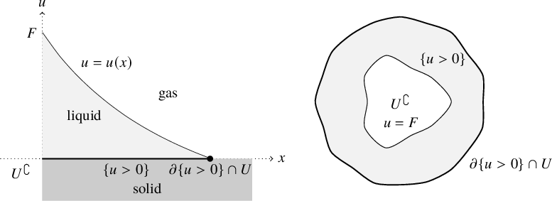


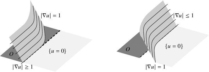


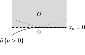

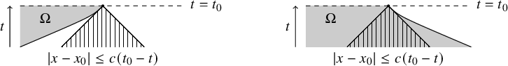


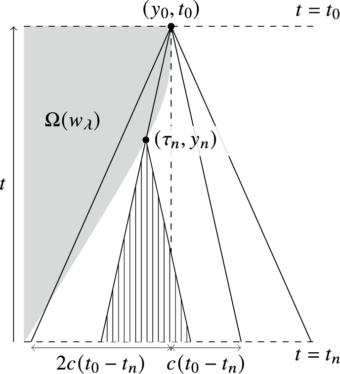


 Open access