


1. Introduction
Active colloids have a prominent position as self-propelling agents that enable the study of multi-agent systems, called ‘active matter’ (Ramaswamy Reference Ramaswamy2010). These canonical systems of active matter serve as micro-engineered analogues of crowds, flocks of birds or bacterial swarms. A common propulsion mechanism is phoresis, where particles move in gradients of a surrounding field (Anderson Reference Anderson1989). This occurs due to short-range interactions between a particle’s surface and the surrounding field that generate an effective slip flow close to the particle’s surface, such as solute concentration (Golestanian, Liverpool & Ajdari Reference Golestanian, Liverpool and Ajdari2005), temperature (Bickel, Majee & Würger Reference Bickel, Majee and Würger2013) or electric field (Nourhani et al. Reference Nourhani, Crespi, Lammert and Borhan2015). If the particle also creates gradients in the surrounding propulsive field, then it can self-propel; this self-propulsion is called autophoresis (Paxton et al. Reference Paxton, Kistler, Olmeda, Sen, Angelo, Cao, Mallouk, Lammert and Crespi2004).
One class of autophoretic particles consists of chemically active (diffusiophoretic) colloids, which are microscale particles that swim by converting a solute ‘fuel’ in their environment into propulsive slip flows (Golestanian, Liverpool & Ajdari Reference Golestanian, Liverpool and Ajdari2007). The canonical chemically active colloid is the ‘Janus’ particle, which is half active and half inert; typically, this takes the form of a rigid sphere, rod or disk, partially coated in a catalyst, such as platinum, in a surrounding solute such as hydrogen peroxide solution (Howse et al. Reference Howse, Jones, Ryan, Gough, Vafabakhsh and Golestanian2007; Ebbens & Howse Reference Ebbens and Howse2011). Differential reaction rates at the particle’s surface create surface gradients in the solute concentration; the resulting short-range solute–surface interactions generate pressure gradients in a thin layer that drives slip flows close to the surface that propel the swimmer.
A natural evolution in the field of active colloids is to consider chemically active filaments. The three-dimensional geometry and the separation of scales into long and thin directions unlocks extra degrees of freedom, functionality and dynamics. This includes localisation of surface flow patterns through the modulation of surface properties and precision-control of their three-dimensional positioning through the centreline shape. Dynamic control of the centreline shape, perhaps using external stimuli, could then be used to individually control the motion and function of slender microbots (Montenegro-Johnson Reference Montenegro-Johnson2018).
Modelling approaches have evolved to predict the benefits of creating slender phoretic microswimmers. Initial phoretic models addressed slender filaments with only straight centrelines, with spheroidal or arbitrary cross-section (Yariv & Schnitzer Reference Yariv and Schnitzer2013; Schnitzer & Yariv Reference Schnitzer and Yariv2015; Michelin & Lauga Reference Michelin and Lauga2017). This was followed by the development of slender phoretic theory (SPT) by Katsamba, Michelin & Montenegro-Johnson (Reference Katsamba, Michelin and Montenegro-Johnson2020), derived using matched asymptotics from a boundary integral formulation. Independently, Poehnl & Uspal (Reference Poehnl and Uspal2021) derived an SPT for curved rods from a more intuitive perspective of distributions of sources and dipoles. The SPT developed in Katsamba et al. (Reference Katsamba, Michelin and Montenegro-Johnson2020, Reference Katsamba, Butler, Koens and Montenegro-Johnson2022, Reference Katsamba and Montenegro-Johnson2024) calculates the induced slip velocities via evaluation of line integrals in the diffusion-dominated regime. The theory is asymptotically accurate for long and thin filaments, and is valid for general non-intersecting three-dimensional filament centrelines, both open-ended and looped. Further, it can accommodate varying circular cross-sectional radius with arbitrary chemical patterning, including discrete jumps in chemical patterning (Katsamba & Montenegro-Johnson Reference Katsamba and Montenegro-Johnson2024). Notably, numerical implementations of SPT (Katsamba et al. Reference Katsamba, Michelin and Montenegro-Johnson2020, Reference Katsamba, Butler, Koens and Montenegro-Johnson2024) are orders of magnitude faster than boundary element methods (Montenegro-Johnson, Michelin & Lauga Reference Montenegro-Johnson, Michelin and Lauga2015), which typically involve a large number of surface integrals.
This previous modelling of chemically propelled filaments has focused on rigid structures with pre-defined, fixed shapes. Realistically, phoretic filaments are not perfectly rigid, and the forces exerted on the body due to relative fluid motion and the chemically generated slip flows may deform the filament, changing its geometry and hence its swimming behaviour. A natural question is therefore: how do flexible phoretic filaments behave dynamically?
Microscale flexible filaments in viscous flows are well studied, due in part to their prevalence in many biological and artificial systems (Lauga & Powers Reference Lauga and Powers2009; Du Roure et al. Reference du Roure, Lindner, Nazockdast and Shelley2019). In biology, carpets of slender filaments, known as cilia, actively pump fluid over cycles driven by internal active forces (Ishikawa Reference Ishikawa2024); sperm cells swim due to active waves sent down their long and thin tail-like appendages (Gaffney et al. Reference Gaffney, Gadêlha, Smith, Blake and Kirkman-Brown2011); and bacteria rotate slender, helical flagella to propel themselves (Lauga Reference Lauga2016). Meanwhile, flexible fibres are present in many industrial and household processes, such as textile fibres in clothing (Duprat Reference Duprat2022), wood pulp fibres in the production of paper (Lundell, Söderberg & Alfredsson Reference Lundell, Söderberg and Alfredsson2011), and microplastics that can pollute the environment (DiBenedetto Reference DiBenedetto2025).
The dynamics of these flexible filaments in viscous flows is difficult to simulate since there is intrinsic feedback between the filament shape, the distribution of forces and the surrounding fluid. Simulations are often computationally expensive because the underlying equations are notoriously numerically stiff, and there are often also accompanying constraints, such as inextensiblity, that must be satisfied throughout the evolution of the system (Du Roure et al. Reference du Roure, Lindner, Nazockdast and Shelley2019). A range of methods have been used to model and simulate the hydrodynamics of slender flexible filaments. Local slender body theories, such as resistive force theory (Hancock Reference Hancock1953; Gray & Hancock Reference Gray and Hancock1955; Batchelor Reference Batchelor1970; Cox Reference Cox1970; Lighthill Reference Lighthill1976), have been applied to generate fast, efficient simulations of elastic filaments (Moreau, Giraldi & Gadêlha Reference Moreau, Giraldi and Gadêlha2018; Walker, Ishimoto & Gaffney Reference Walker, Ishimoto and Gaffney2020), while non-local slender body theories (Keller & Rubinow Reference Keller and Rubinow1976; Johnson Reference Johnson1977, Reference Johnson1980; Koens & Lauga Reference Koens and Lauga2018) provide greater accuracy through more intensive simulations (Tornberg & Shelley Reference Tornberg and Shelley2004). Alternative approaches involve using singularity methods such as regularised Stokeslets (Cortez Reference Cortez2001; Cortez, Fauci & Medovikov Reference Cortez, Fauci and Medovikov2005; Hall-McNair et al. Reference Hall-McNair, Montenegro-Johnson, Gadêlha, Smith and Gallagher2019), immersed boundary methods (Pozrikidis Reference Pozrikidis1992; Peskin Reference Peskin2002) and bead models (Delmotte, Climent & Plouraboué (Reference Delmotte, Climent and Plouraboué2015), and references therein). These models have been developed further to investigate the interaction of flexible fibres and the behaviour of passive and active suspensions (Tornberg & Shelley Reference Tornberg and Shelley2004; Schoeller et al. Reference Schoeller, Townsend, Westwood and Keaveny2021).
Elastic filaments demonstrate a wide range of interesting and exciting behaviours, depending on the strength of applied forces relative to the stiffness of the material. As summarised in the review of Du Roure et al. (Reference du Roure, Lindner, Nazockdast and Shelley2019), as the strength of external forcing or the flexibility of passive fibres in a flow increases, the dynamics progresses from behaving as rigid rods, to undergoing buckling instabilities, folding through hook shapes, and contorting out of plane, depending on the prescribed flow and surrounding environment.
Active fibres have also been found to undergo similar dynamic transitions depending on the strength of activity relative to the fibre stiffness, with a particular focus on clamped filaments as models of ciliary beating or actin filaments. Bead–spring models of a chain of elastically linked beads, such as with stresslets distributed along its axis (Laskar et al. Reference Laskar, Singh, Ghose, Jayaraman, Kumar and Adhikari2013) or when forced at one end (Laskar & Adhikari Reference Laskar and Adhikari2017), demonstrated whirling, corkscrewing and planar beating dynamics; similar linear, helical and planar modes were found when attached to a passive cargo (Manna, Kumar & Adhikari Reference Michelin and Lauga2017). This bead–spring approach has recently been extended to finer resolution to investigate active poroelastic filaments under ‘follower’ forces that act tangentially to the centreline at the free end of the filament (Altunkeyik, Rahmat & Montenegro-Johnson Reference Altunkeyik, Rahmat and Montenegro-Johnson2025), which showed rich transitions between dynamic behaviours, including for chemically active poroelastic filaments, and exhibited regimes of periodic and diffusive-like motion.
An alternative approach to studying active elastohydrodynamics is to combine resistive force theory with the mechanics of elastic filaments. When the motion is confined to lie in the plane, filaments deforming due to follower forces have been shown to undergo Hopf bifurcations, seen as a flapping motion for clamped filaments (De Canio et al. Reference De Canio, Lauga and Goldstein2017), while a two-dimensional linear stability analysis revealed transitions to rotation or beating that depend on mechanical boundary conditions, applied load, and noise effects (Fily et al. Reference Fily, Subramanian, Schneider, Chelakkot and Gopinath2020). Further dynamical regimes have been explored using this elastohydrodynamic theory when applying localised tangential forces (Man & Kanso Reference Man and Kanso2019) to extract motions such as straight swimming, circling, spiralling and undulating, and also with clamped filaments in confined domains (Stein et al. Reference Stein, De Canio, Lauga, Shelley and Goldstein2021), revealing transitions of filaments with distributed tangential forces from stable to oscillatory and streaming modes. Recent theoretical contributions by Clarke, Hwang & Keaveny (Reference Clarke, Hwang and Keaveny2024) and Schnitzer (Reference Schnitzer2025) further investigate the full three-dimensional motion of these follower-force models, identifying beating and whirling onset via bifurcation theory and weakly nonlinear analysis, enriching the fundamental understanding of these dynamics. Interestingly, clamped filaments that are free to deform in three dimensions display a non-planar ‘whirling’ motion following the onset of instability, and reach a planar beating state only when the applied force is much stronger. In a related system, Lough, Weibel & Spagnolie (Reference Lough, Weibel and Spagnolie2023) modelled the swarmer cell state of Proteus mirabilis as an active Kirchhoff rod, and found different swimming modes that may be planar or twisted into three dimensions, depending on the relative material stiffnesses. Although many of these models abstract away the details provided by the surface chemistry of phoretic propulsion, e.g. by using follower forces, we expect that they retain essential features of force-induced shape transformations and the resulting complex locomotion, and highlight the complex interplay of elasticity, active forcing and boundary conditions in shaping filament dynamics.
Recently, Makanga, Varma & Katsamba (Reference Makanga, Varma and Katsamba2025) conducted a detailed linear stability analysis of planar, uniformly active elastohydrodynamic filaments with phoretic slip flows, focusing exclusively on motion confined to a plane. Through numerical and analytical exploration, they identified the onset of planar buckling of uniformly active filaments, which led to net motion of otherwise immotile phoretic slender bodies. In this study, we move beyond planar motion by combining SPT (Katsamba et al. Reference Katsamba, Michelin and Montenegro-Johnson2020, Reference Katsamba, Butler, Koens and Montenegro-Johnson2022, Reference Katsamba, Butler, Koens and Montenegro-Johnson2024) with recent advances in the efficient simulation of elastohydrodynamic filaments in three spatial dimensions (Walker et al. Reference Walker, Ishimoto and Gaffney2020). This leads us beyond the planar buckling problem and enables exploration of rich, truly three-dimensional behaviours. We consider examples of canonical surface chemical patterning to study the transition between a range of qualitatively different dynamic regimes as the relative strength of the phoretic activity is varied, including a three-dimensional buckling phenomenon that drives dynamics out of the plane. Section 2 outlines our theoretical method and numerical implementation for modelling chemically active filaments, using a local slender body theory to calculate the resulting slip flows from chemical reactions on the filament’s surface, which are applied as a boundary condition in the numerical simulations of the elastohydrodynamics. We present our results in § 3, investigating typical behaviours via two key examples: a symmetrically patterned filament that buckles under its own induced slip flow, and an asymmetrically patterned filament whose swimming trajectory is altered by its deformation. We discuss and analyse the outcomes further in § 4.
2. Theory of chemoelastohydrodynamic filaments
A slender chemically active elastic filament in an infinite fluid bath. The filament geometry is captured by a centreline $\boldsymbol{X}(s)$
, parametrised by its arc length
$\boldsymbol{X}(s)$
, parametrised by its arc length $s$
, with local polar coordinates on any circular cross-section given by
$s$
, with local polar coordinates on any circular cross-section given by $(\rho ,\theta )$
. Chemical patterning can vary across the surface of the filament, as shown by the filament colour, and generates solute at rate
$(\rho ,\theta )$
. Chemical patterning can vary across the surface of the filament, as shown by the filament colour, and generates solute at rate $\mathcal{A}(s,\theta )$
. Any resulting surface solute concentration gradients generate a slip flow that moves the surrounding fluid and applies viscous forces on the filament that can propel and deform it.
$\mathcal{A}(s,\theta )$
. Any resulting surface solute concentration gradients generate a slip flow that moves the surrounding fluid and applies viscous forces on the filament that can propel and deform it.

We consider an inextensible slender elastic filament in an otherwise quiescent, infinite viscous fluid, as shown in figure 1. Within the fluid is a chemical solute that diffuses rapidly. The solute acts as a fuel for the filament’s self-propulsion: a chemical reaction of the solute dispersed in the surrounding fluid is catalysed by the catalytic coating on the surface of the filament, and short-range interactions between solute molecules and the filament’s surface generate propulsive slip flows from solute concentration gradients within a thin layer by the filament’s surface. The resulting bulk flow can propel and deform the filament, altering the filament conformation and changing the solute distribution; there is a complex feedback between shape, chemical patterning and swimming trajectory that we wish to explore.
Here, we outline the main theoretical components used to capture the evolution of slender chemically propelled elastic filaments. Our work combines two pre-existing methods: SPT (Katsamba et al. Reference Katsamba, Michelin and Montenegro-Johnson2020, Reference Katsamba, Butler, Koens and Montenegro-Johnson2022, Reference Katsamba, Butler, Koens and Montenegro-Johnson2024; Katsamba & Montenegro-Johnson Reference Katsamba and Montenegro-Johnson2024), which asymptotically calculates the leading-order slip flow around slender chemically active filaments when given their chemical patterning and shape, and an efficient method for simulating elastohydrodynamics (Walker et al. Reference Walker, Ishimoto and Gaffney2020). Together, these allow us to probe the dynamic behaviour of chemically propelled elastic filaments, which we refer to as chemoelastohydrodynamics.
2.1. The slender filament geometry
The geometry of a slender filament with a circular cross-section is captured by its centreline position $\boldsymbol{X}(s,t)$
and cross-sectional radius
$\boldsymbol{X}(s,t)$
and cross-sectional radius $\rho (s)$
, each parametrised by the arc length
$\rho (s)$
, each parametrised by the arc length $s$
such that
$s$
such that $|\partial \boldsymbol{X}/\partial s|=1$
. The filament centreline has total length
$|\partial \boldsymbol{X}/\partial s|=1$
. The filament centreline has total length $2{l}$
, and the maximum cross-sectional radius is
$2{l}$
, and the maximum cross-sectional radius is $r_{\!f}$
; and we assume that the filament is unshearable, so that cross-sections remain perpendicular to the centreline. We define a slenderness parameter by the ratio of the maximum diameter to the total arc length,
$r_{\!f}$
; and we assume that the filament is unshearable, so that cross-sections remain perpendicular to the centreline. We define a slenderness parameter by the ratio of the maximum diameter to the total arc length, $\epsilon =r_{\!f}/{l}$
, which can be considered an aspect ratio, and we assume that our filaments are long and thin so that
$\epsilon =r_{\!f}/{l}$
, which can be considered an aspect ratio, and we assume that our filaments are long and thin so that $\epsilon \ll 1$
.
$\epsilon \ll 1$
.
The surface of the filament is patterned with two important surface chemical properties: the activity $\mathcal{A}({\boldsymbol{x}})$
, which prescribes a surface solute flux (either generating or depleting solute), and the mobility
$\mathcal{A}({\boldsymbol{x}})$
, which prescribes a surface solute flux (either generating or depleting solute), and the mobility $\mathcal{M}({\boldsymbol{x}})$
, which quantifies how chemical gradients drive slip flows. Theoretically, we can set these independently, and they may vary over the surface, but we assume that the distribution remains fixed in the material frame.
$\mathcal{M}({\boldsymbol{x}})$
, which quantifies how chemical gradients drive slip flows. Theoretically, we can set these independently, and they may vary over the surface, but we assume that the distribution remains fixed in the material frame.
The system is non-dimensionalised: spatial coordinates are rescaled by the half-length of the filament $l$
, while the cross-sectional radius is rescaled by the maximum radius
$l$
, while the cross-sectional radius is rescaled by the maximum radius $r_{\!f}$
. Taking typical (maximum) values for the activity and mobility as
$r_{\!f}$
. Taking typical (maximum) values for the activity and mobility as $A$
and
$A$
and $M$
, respectively, we also use a concentration scale
$M$
, respectively, we also use a concentration scale $Ar_{\!f}/D$
and a velocity scale
$Ar_{\!f}/D$
and a velocity scale $AMr_{\!f}/ D {l}$
to rescale our equations, where
$AMr_{\!f}/ D {l}$
to rescale our equations, where $D$
is the diffusivity of the solute. All equations are henceforth given in dimensionless form.
$D$
is the diffusivity of the solute. All equations are henceforth given in dimensionless form.
2.2. Local SPT
The slip flow generated by the chemical activity is calculated using SPT. The full details of this asymptotically accurate theory are given in Katsamba et al. (Reference Katsamba, Michelin and Montenegro-Johnson2020, Reference Katsamba, Butler, Koens and Montenegro-Johnson2022, Reference Katsamba, Butler, Koens and Montenegro-Johnson2024) and Katsamba & Montenegro-Johnson (Reference Katsamba and Montenegro-Johnson2024); here, we outline the key points.
We consider the zero Péclet number limit for the solute dynamics, where diffusion dominates advection, so that the solute concentration $c$
in the surrounding fluid is governed by Laplace’s equation,
$c$
in the surrounding fluid is governed by Laplace’s equation,
 \begin{equation} {\nabla} ^2 c = 0, \end{equation}
where we consider the disturbance from a background concentration, so that $c\to 0$
far from the surface.
$c\to 0$
far from the surface.
The activity provides a normal flux boundary condition at the filament surface via zeroth-order reaction kinetics, and any resulting surface concentration gradients drive the slip flow proportional to the mobility. These are boundary conditions on the surface of the filament:
 \begin{align} -\boldsymbol{n}_{\!f}\boldsymbol{\cdot }\boldsymbol{\nabla } c &= \mathcal{A}(\boldsymbol{x}), \end{align}
 \begin{align} \boldsymbol{v}_{\textit{slip}} &= \mathcal{M}({\boldsymbol{x}}) \left (\boldsymbol{1} - \boldsymbol{n}_{\!f} \boldsymbol{n}_{\!f} \right )\boldsymbol{\cdot }\boldsymbol{\nabla } c, \end{align}
where $\boldsymbol{n}_{\!f}$
is the outward normal to the solid surface. Importantly, we frame our results in terms of the arc length
$\boldsymbol{n}_{\!f}$
is the outward normal to the solid surface. Importantly, we frame our results in terms of the arc length $s$
and local polar coordinates in the cross-section
$s$
and local polar coordinates in the cross-section $(r,\theta )$
. Surface properties are therefore defined by the arc length
$(r,\theta )$
. Surface properties are therefore defined by the arc length $s\in [-1,1]$
along the centreline, and angle
$s\in [-1,1]$
along the centreline, and angle $\theta \in [-\pi ,\pi ]$
around the cross-section, i.e.
$\theta \in [-\pi ,\pi ]$
around the cross-section, i.e. $\mathcal{A}=\mathcal{A}(s,\theta )$
and
$\mathcal{A}=\mathcal{A}(s,\theta )$
and $\mathcal{M}=\mathcal{M}(s,\theta )$
, with the surface at
$\mathcal{M}=\mathcal{M}(s,\theta )$
, with the surface at $r=\rho (s)\in [0,1]$
. Note that we take
$r=\rho (s)\in [0,1]$
. Note that we take $\theta$
as the angle relative to a fixed position in each cross-section in the material frame. These local coordinates are shown in the inset to figure 1.
$\theta$
as the angle relative to a fixed position in each cross-section in the material frame. These local coordinates are shown in the inset to figure 1.
In the framework of SPT (Katsamba et al. Reference Katsamba, Michelin and Montenegro-Johnson2020, Reference Katsamba, Butler, Koens and Montenegro-Johnson2022, Reference Katsamba, Butler, Koens and Montenegro-Johnson2024; Katsamba & Montenegro-Johnson Reference Katsamba and Montenegro-Johnson2024), the solution of Laplace’s equation for the solute concentration is derived via a matched-asymptotics expansion in the slenderness $\epsilon$
on the boundary integral solution of Laplace’s equation. This method systematically reduces the problem from solving an implicit indirect surface integral equation over the filament to a significantly simpler explicit calculation of a line integral along the filament centreline. This non-local slender theory for chemically active filaments is valid for arbitrary non-self-intersecting three-dimensional centrelines, and can deal with both varying thickness and non-axisymmetric chemical patterning. For this, the surface solute concentration is expanded as
$\epsilon$
on the boundary integral solution of Laplace’s equation. This method systematically reduces the problem from solving an implicit indirect surface integral equation over the filament to a significantly simpler explicit calculation of a line integral along the filament centreline. This non-local slender theory for chemically active filaments is valid for arbitrary non-self-intersecting three-dimensional centrelines, and can deal with both varying thickness and non-axisymmetric chemical patterning. For this, the surface solute concentration is expanded as
 \begin{align} c(s,\theta ) = {c}^{(0)}(s,\theta ;\epsilon ) + \epsilon\, {c}^{(1)}(s,\theta ;\epsilon ) + o(\epsilon ), \end{align}
where the terms ${c}^{(0)},\,{c}^{(1)}$
are allowed to depend weakly (i.e. logarithmically) upon
${c}^{(0)},\,{c}^{(1)}$
are allowed to depend weakly (i.e. logarithmically) upon $\epsilon$
. The resulting slip velocity over the surface of the swimmer can then be determined as a surface gradient of the concentration:
$\epsilon$
. The resulting slip velocity over the surface of the swimmer can then be determined as a surface gradient of the concentration:
 \begin{align} \frac {\boldsymbol{v}_{\textit{slip}}(s,\theta )}{\mathcal{M}(s,\theta )} =& \underbrace { \frac {\hat {\boldsymbol{e}}_{\theta }(s,\theta )}{\epsilon\, \rho (s)} \frac {\partial {c}^{(0)}}{\partial \theta } }_{O(1/\epsilon )} +\underbrace {\left [ \frac {\hat {\boldsymbol{e}}_{\theta }(s,\theta )}{ \rho } \frac {\partial {c}^{(1)}}{\partial \theta } + \hat {\boldsymbol{t}}(s) \frac {\partial {c}^{(0)}}{\partial s} \right ]}_{O(1)} + \,o(1), \end{align}
where $\hat {\boldsymbol{t}}(s)$
is the tangent to the centreline, and
$\hat {\boldsymbol{t}}(s)$
is the tangent to the centreline, and $\hat {\boldsymbol{e}}_{\theta }(s,\theta )$
is the unit vector pointing azimuthally around the cross-section. Note that gradients in concentration in the azimuthal direction around a cross-section, i.e. in the
$\hat {\boldsymbol{e}}_{\theta }(s,\theta )$
is the unit vector pointing azimuthally around the cross-section. Note that gradients in concentration in the azimuthal direction around a cross-section, i.e. in the $\theta$
direction, are magnified by a factor
$\theta$
direction, are magnified by a factor $1/\epsilon$
in the slip velocity.
$1/\epsilon$
in the slip velocity.
In this work, we focus on axisymmetric activities, with $\mathcal{A} = \mathcal{A}(s)$
. Katsamba et al. (Reference Katsamba, Michelin and Montenegro-Johnson2020) showed that this leads to axisymmetric surface concentration at leading order, which is independent of
$\mathcal{A} = \mathcal{A}(s)$
. Katsamba et al. (Reference Katsamba, Michelin and Montenegro-Johnson2020) showed that this leads to axisymmetric surface concentration at leading order, which is independent of $\theta$
,
$\theta$
, ${c}^{(0)} = {c}^{(0)}(s)$
, so that the
${c}^{(0)} = {c}^{(0)}(s)$
, so that the $O(1/\epsilon )$
term in (2.5) is identically zero. Hence both
$O(1/\epsilon )$
term in (2.5) is identically zero. Hence both ${c}^{(0)}(s)$
and
${c}^{(0)}(s)$
and ${c}^{(1)}(s,\theta )$
contribute to the leading-order slip velocity at
${c}^{(1)}(s,\theta )$
contribute to the leading-order slip velocity at $O(1)$
. Expressions for these terms are computed explicitly in Katsamba et al. (Reference Katsamba, Michelin and Montenegro-Johnson2020).
$O(1)$
. Expressions for these terms are computed explicitly in Katsamba et al. (Reference Katsamba, Michelin and Montenegro-Johnson2020).
Consistent with the local drag theory that we will use to couple the motion to the fluid, described in § 2.3, here we employ a local approximation of SPT. In this systematic, leading-order reduction of the theory, we retain only the local (non-integral) terms in the expressions for ${c}^{(0)}(s)$
and
${c}^{(0)}(s)$
and ${c}^{(1)}(s,\theta )$
given in Appendix A; the neglected integral terms are
${c}^{(1)}(s,\theta )$
given in Appendix A; the neglected integral terms are $O(1/\log {\epsilon })$
smaller than the local terms. This leads to an expression for
$O(1/\log {\epsilon })$
smaller than the local terms. This leads to an expression for $\boldsymbol{v}_{\textit{slip}}(s,\theta )$
that is accurate at leading order.
$\boldsymbol{v}_{\textit{slip}}(s,\theta )$
that is accurate at leading order.
The local contributions of ${c}^{(0)}(s)$
and
${c}^{(0)}(s)$
and ${c}^{(1)}(s,\theta )$
used to approximate the slip velocity
${c}^{(1)}(s,\theta )$
used to approximate the slip velocity $\boldsymbol{v}_{\textit{slip}}(s,\theta )$
are
$\boldsymbol{v}_{\textit{slip}}(s,\theta )$
are
 \begin{align} {c}^{(0)}(s) &= \frac {1}{2} \rho (s)\,\mathcal{A}(s)\log \left (\frac {4\bigl(1-s^2\bigr) }{\epsilon ^2\, \rho ^2(s)}\right )\!, \end{align}
 \begin{align} {c}^{(1)}(s,\theta ) &= \frac {1}{2} \rho ^2(s)\, \kappa (s)\, \mathcal{A}(s) \cos \varTheta (s,\theta ) \left [\log \left (\frac {4\bigl(1-s^2\bigr)}{\epsilon ^2\, \rho ^2(s)} \right ) - 3\right ]\!, \end{align}
where $\kappa$
is the Frenet–Serret curvature, and
$\kappa$
is the Frenet–Serret curvature, and $\varTheta$
is the azimuthal angle relative to the Frenet–Serret basis, tracking the azimuthal angle relative to the cumulative torsion. (Note that
$\varTheta$
is the azimuthal angle relative to the Frenet–Serret basis, tracking the azimuthal angle relative to the cumulative torsion. (Note that $\varTheta$
is not fixed relative to the material frame, and the Frenet–Serret normal coincides with
$\varTheta$
is not fixed relative to the material frame, and the Frenet–Serret normal coincides with $\varTheta =0$
.) We validate the resulting approximation for the slip velocity in Appendix B, finding good agreement. Notably, were one to use these expressions for
$\varTheta =0$
.) We validate the resulting approximation for the slip velocity in Appendix B, finding good agreement. Notably, were one to use these expressions for ${c}^{(0)}$
and
${c}^{(0)}$
and ${c}^{(1)}$
directly in (2.4), the expansion would not be asymptotically consistent, as the neglected integral in
${c}^{(1)}$
directly in (2.4), the expansion would not be asymptotically consistent, as the neglected integral in ${c}^{(0)}$
would be larger than the
${c}^{(0)}$
would be larger than the $O(\epsilon )$
contribution of
$O(\epsilon )$
contribution of ${c}^{(1)}$
.
${c}^{(1)}$
.
Further, to determine the leading-order kinematics of the filament, it is only necessary to calculate the cross-sectional average of the slip velocity, since all higher-order modes in a Fourier series in $\theta$
have smaller effects in the motion of the slender body (see e.g. Katsamba et al. Reference Katsamba, Michelin and Montenegro-Johnson2020, § 2.9). This is consistent with our use of the Kirchhoff rod equations (see § 2.4), which require only the net force and torque on the centreline, which in turn can be calculated from the cross-sectionally averaged slip flow (Koens & Lauga Reference Koens and Lauga2018). The slip velocity calculation can then be further simplified by decomposing
$\theta$
have smaller effects in the motion of the slender body (see e.g. Katsamba et al. Reference Katsamba, Michelin and Montenegro-Johnson2020, § 2.9). This is consistent with our use of the Kirchhoff rod equations (see § 2.4), which require only the net force and torque on the centreline, which in turn can be calculated from the cross-sectionally averaged slip flow (Koens & Lauga Reference Koens and Lauga2018). The slip velocity calculation can then be further simplified by decomposing $\hat {\boldsymbol{e}}_{\theta }$
into Frenet–Serret normal and binormal vectors, so that we find the cross-sectional average slip velocity to be
$\hat {\boldsymbol{e}}_{\theta }$
into Frenet–Serret normal and binormal vectors, so that we find the cross-sectional average slip velocity to be
 \begin{equation} \bar {\boldsymbol{v}}_{slip}(s) \equiv \frac {1}{2\pi } \int _{-\pi }^{\pi } \boldsymbol{v}_{\textit{slip}}(s,\tilde {\theta }) \,{\mathrm{d}} \tilde {\theta } = \mathcal{M}(s) \left [ \hat {\boldsymbol{t}}(s) \frac {\partial {c}^{(0)}}{\partial s} -\frac {1}{2}\hat {\boldsymbol{n}}(s)\,A_s(s) \right ]\! , \end{equation}
where $\hat {\boldsymbol{n}}(s)$
is the Frenet–Serret normal, and
$\hat {\boldsymbol{n}}(s)$
is the Frenet–Serret normal, and
 \begin{equation} A_s(s)= - \frac {1}{2}\left [\log \left (\frac {4\bigl(1-s^2\bigr)}{\epsilon ^2\, \rho ^2(s)}\right ) -3\right ]\rho (s)\,\kappa (s)\,\mathcal{A}(s). \end{equation}
2.3. Resistive force theory
The phoretic slip flow induces bulk flow in the surrounding fluid, acting as a boundary condition to the Stokes equations for a viscous fluid:
 \begin{equation} \mu {\nabla} ^2 \boldsymbol{u} = \boldsymbol{\nabla }p, \quad \boldsymbol{\nabla }\boldsymbol{\cdot }\boldsymbol{u} = 0, \end{equation}
where $\boldsymbol{u}(\boldsymbol{x},t)$
is the fluid velocity,
$\boldsymbol{u}(\boldsymbol{x},t)$
is the fluid velocity, $p(\boldsymbol{x},t)$
is the fluid pressure, and
$p(\boldsymbol{x},t)$
is the fluid pressure, and $\mu$
is the fluid’s dynamic viscosity. The flow is assumed to decay to
$\mu$
is the fluid’s dynamic viscosity. The flow is assumed to decay to $\boldsymbol{u}=\boldsymbol{0}$
in the far field, and satisfies a prescribed slip boundary condition on the surface of the body, with
$\boldsymbol{u}=\boldsymbol{0}$
in the far field, and satisfies a prescribed slip boundary condition on the surface of the body, with
 \begin{equation} \boldsymbol{u}\vert _{\textit{surface}}(s,\theta ) = \frac {\partial \boldsymbol{X}}{\partial t} + \boldsymbol{\varOmega }(s)\wedge \hat {\boldsymbol{e}}_{\rho }(s,\theta ) + \boldsymbol{v}_{\textit{slip}}(s,\theta ) \end{equation}
on the surface, where $\boldsymbol{\varOmega }(s)$
is the (implicitly time-dependent) rate of local rotation of the slender body about the centreline. This slip condition is consistent with the idea that slip velocities act in the direction opposite to the motion that they drive; for example, a force-free cylinder with slip moves at a speed given by the surface average of the slip velocity, but in the opposite direction, as can be shown by application of the reciprocal theorem for Stokes flow. It is convenient to decompose the surface velocity into its cross-sectional average and the angle-dependent components, defining
$\boldsymbol{\varOmega }(s)$
is the (implicitly time-dependent) rate of local rotation of the slender body about the centreline. This slip condition is consistent with the idea that slip velocities act in the direction opposite to the motion that they drive; for example, a force-free cylinder with slip moves at a speed given by the surface average of the slip velocity, but in the opposite direction, as can be shown by application of the reciprocal theorem for Stokes flow. It is convenient to decompose the surface velocity into its cross-sectional average and the angle-dependent components, defining
 \begin{equation} \bar {\boldsymbol{u}}\vert _{\textit{surface}}(s) \equiv \frac {1}{2\pi } \int _{-\pi }^{\pi } \boldsymbol{u}\vert _{\textit{surface}}(s,\tilde {\theta }) \,{\mathrm{d}} \tilde {\theta } = \frac {\partial \boldsymbol{X}}{\partial t} + \bar {\boldsymbol{v}}_{slip}(s). \end{equation}
As noted in § 2.2, at leading order in $\epsilon$
, we can neglect the angle-dependent components of
$\epsilon$
, we can neglect the angle-dependent components of $\boldsymbol{v}_{\textit{slip}}(s,\theta )$
in favour of
$\boldsymbol{v}_{\textit{slip}}(s,\theta )$
in favour of $\bar {\boldsymbol{v}}_{slip}(s)$
; hence the angle-dependent component of the velocity boundary condition reduces to
$\bar {\boldsymbol{v}}_{slip}(s)$
; hence the angle-dependent component of the velocity boundary condition reduces to
 \begin{equation} \boldsymbol{u}\vert _{\textit{surface}}(s,\theta ) - \bar {\boldsymbol{u}}\vert _{\textit{surface}}(s) \sim \boldsymbol{\varOmega }(s)\wedge \hat {\boldsymbol{e}}_{\rho }(s,\theta ), \end{equation}
corresponding to local rotation at leading order.
To relate flows to forces, we use resistive force theory (Hancock Reference Hancock1953; Gray & Hancock Reference Gray and Hancock1955). This is a systematically constructed, logarithmically accurate local slender body theory for viscous flow that decomposes the local motion of the filament (relative to a background or slip flow) into components that are locally tangential and normal to the centreline, linearly relating the leading-order force density and velocity of each via different drag coefficients. For tangential and normal components ( $\boldsymbol{u}_\parallel$
and
$\boldsymbol{u}_\parallel$
and $\boldsymbol{u}_\perp$
, respectively) of the cross-sectionally averaged translational flow
$\boldsymbol{u}_\perp$
, respectively) of the cross-sectionally averaged translational flow $\bar {\boldsymbol{u}}\vert _{\textit{surface}}(s)$
, resistive force theories state
$\bar {\boldsymbol{u}}\vert _{\textit{surface}}(s)$
, resistive force theories state
 \begin{equation} \boldsymbol{f}_\parallel = - C_\parallel \boldsymbol{u}_\parallel , \quad \boldsymbol{f}_\perp = - C_\perp \boldsymbol{u}_\perp , \end{equation}
where $\boldsymbol{f}_\parallel , \boldsymbol{f}_\perp$
denote the force densities applied on the filament in directions tangential to the centreline and normal to it. The drag coefficients
$\boldsymbol{f}_\parallel , \boldsymbol{f}_\perp$
denote the force densities applied on the filament in directions tangential to the centreline and normal to it. The drag coefficients $C_\parallel$
and
$C_\parallel$
and $C_\perp$
used in this study are those of Gray & Hancock (Reference Gray and Hancock1955), given by
$C_\perp$
used in this study are those of Gray & Hancock (Reference Gray and Hancock1955), given by
 \begin{equation} C_\parallel = \frac {2\pi \mu }{\log (4/\rho \epsilon )-0.5}, \quad C_\perp = \frac {4\pi \mu }{\log (4/\rho \epsilon )-0.5}. \end{equation}
Note that our application of resistive force theory to slip boundary conditions is valid for the slip flows generated by chemically propelled filaments, since local slender body theories are consistent with boundary conditions that enforce rigid body motion locally, as is the case here (Walker, Ishimoto & Gaffney Reference Walker, Ishimoto and Gaffney2023).
The resistive torque theory of Walker et al. (Reference Walker, Ishimoto and Gaffney2023) links local angular velocity (such as that about the local tangent) to local torque via an additional resistive coefficient, allowing us to capture the remainder of the velocity boundary condition. Following this, the leading-order, locally applied torque per unit length is given by
 \begin{equation} \boldsymbol{\tau }=4\pi \epsilon ^2\,\rho^2 (s)\,\mu \boldsymbol{\varOmega }, \end{equation}
where $\boldsymbol{\varOmega }$
is the angular velocity of the slender body from (2.10) and (2.12). This torque will often be negligible, as an
$\boldsymbol{\varOmega }$
is the angular velocity of the slender body from (2.10) and (2.12). This torque will often be negligible, as an $O(1)$
rotation rate leads to
$O(1)$
rotation rate leads to $O(\epsilon ^2)$
torques; however,
$O(\epsilon ^2)$
torques; however, $O(1)$
torques correspond to non-negligible angular velocities, as might arise from initially twisted slender bodies, for instance. Though we do not initially twist the slender bodies considered in this work, we retain this explicit coupling between local rotation and torque (rather than employing a suitable quasi-steady-state assumption) in pursuit of generality and to avoid introducing an additional approximation to the framework; it also proves to be convenient for the numerical simulation of the slender body dynamics.
$O(1)$
torques correspond to non-negligible angular velocities, as might arise from initially twisted slender bodies, for instance. Though we do not initially twist the slender bodies considered in this work, we retain this explicit coupling between local rotation and torque (rather than employing a suitable quasi-steady-state assumption) in pursuit of generality and to avoid introducing an additional approximation to the framework; it also proves to be convenient for the numerical simulation of the slender body dynamics.
2.4. Kirchhoff rod equations
We model the deformation of the filament using the Kirchhoff equations, which are the pointwise force and moment balance equations
 \begin{align} \frac {\partial \boldsymbol{F}}{\partial s} + \boldsymbol{f} &= \boldsymbol{0}, \end{align}
 \begin{align} \frac {\partial \boldsymbol{M}}{\partial s} + \hat {\boldsymbol{t}}\wedge \boldsymbol{F} + \boldsymbol{\tau } &=\boldsymbol{0}, \end{align}
where $\boldsymbol{F}$
is the internal force acting on the cross-section of the rod at
$\boldsymbol{F}$
is the internal force acting on the cross-section of the rod at $s$
, and
$s$
, and $\boldsymbol{M}$
is the bending moment. We identify
$\boldsymbol{M}$
is the bending moment. We identify $\boldsymbol{f}$
and
$\boldsymbol{f}$
and $\boldsymbol{\tau }$
as the force and torque densities due to the viscous tractions generated by the flow; these are computed using the resistive force framework of § 2.3. Specifically, the tangential and normal components of
$\boldsymbol{\tau }$
as the force and torque densities due to the viscous tractions generated by the flow; these are computed using the resistive force framework of § 2.3. Specifically, the tangential and normal components of $\boldsymbol{f}$
are calculated from (2.13), and
$\boldsymbol{f}$
are calculated from (2.13), and $\boldsymbol{\tau }$
is found from (2.15).
$\boldsymbol{\tau }$
is found from (2.15).
We impose conditions of zero force and torque at the filament ends, so that
 \begin{align} \boldsymbol{F}(-1) = \boldsymbol{F}(1) = \boldsymbol{M}(-1) = \boldsymbol{M}(1) = 0. \end{align}
Integrating (2.16) and (2.17) leads to the governing equations
 \begin{align} \int _{-1}^{1} \boldsymbol{f}(\tilde {s}) \,{\mathrm{d}}\tilde {s} &= 0, \end{align}
 \begin{align} \int _{s}^{1} [\boldsymbol{X}(\tilde {s})-\boldsymbol{X}(s)] \times \boldsymbol{f}(\tilde {s}) + \boldsymbol{\tau }(\tilde {s}) \,{\mathrm{d}}\tilde {s} &= \boldsymbol{M}(s). \end{align}
The bending moment is given by the constitutive equation
 \begin{align} \boldsymbol{M} = EI \left ( \kappa _1 \boldsymbol{d}_{1} + \kappa _2 \boldsymbol{d}_{2} + \frac {\kappa _3}{1+\nu } \boldsymbol{d}_{3} \right )\!, \end{align}
where the $\boldsymbol{d}_{i}$
are a right-handed orthonormal director basis with
$\boldsymbol{d}_{i}$
are a right-handed orthonormal director basis with $\boldsymbol{d}_{3}=\hat {\boldsymbol{t}}$
, and the
$\boldsymbol{d}_{3}=\hat {\boldsymbol{t}}$
, and the $\kappa _i$
are the components of the twist vector such that
$\kappa _i$
are the components of the twist vector such that $\partial \boldsymbol{d}_{i}/\partial s = \boldsymbol{\kappa }\times \boldsymbol{d}_{i}$
. The material parameters are captured by the bending stiffness
$\partial \boldsymbol{d}_{i}/\partial s = \boldsymbol{\kappa }\times \boldsymbol{d}_{i}$
. The material parameters are captured by the bending stiffness $EI$
and the Poisson ratio
$EI$
and the Poisson ratio $\nu$
; for simplicity, we assume that both of these are constant throughout the filament, with
$\nu$
; for simplicity, we assume that both of these are constant throughout the filament, with $\nu =1$
(Nizette & Goriely Reference Nizette and Goriely1999; Antman Reference Antman2005).
$\nu =1$
(Nizette & Goriely Reference Nizette and Goriely1999; Antman Reference Antman2005).
2.5. Numerical implementation
To solve this system numerically, we discretise the slender body into $N$
straight segments of equal length. We assign a local orthonormal director basis to each segment, fixed in the body so that it tracks the material deformation of the body. These director bases are parametrised using Euler angles, employing independent coordinate systems for each segment. Necessarily, this introduces singularities in the parametrisation that may be identified with the poles of canonical spherical polar coordinate systems and related to the gimbal lock phenomenon. These singularities are sidestepped numerically following the method of Walker et al. (Reference Walker, Ishimoto and Gaffney2020): during the dynamics, when any of the Euler angles approaches the singularities of their respective coordinate system, a new coordinate system is chosen for each segment such that the poles are maximally distant from the current configuration. In effect, this adaptive reparametrisation enables us to utilise the convenience of an Euler-angle parametrisation whilst avoiding the singularities associated with this approach.
$N$
straight segments of equal length. We assign a local orthonormal director basis to each segment, fixed in the body so that it tracks the material deformation of the body. These director bases are parametrised using Euler angles, employing independent coordinate systems for each segment. Necessarily, this introduces singularities in the parametrisation that may be identified with the poles of canonical spherical polar coordinate systems and related to the gimbal lock phenomenon. These singularities are sidestepped numerically following the method of Walker et al. (Reference Walker, Ishimoto and Gaffney2020): during the dynamics, when any of the Euler angles approaches the singularities of their respective coordinate system, a new coordinate system is chosen for each segment such that the poles are maximally distant from the current configuration. In effect, this adaptive reparametrisation enables us to utilise the convenience of an Euler-angle parametrisation whilst avoiding the singularities associated with this approach.
We direct the interested reader to the work of Walker et al. (Reference Walker, Ishimoto and Gaffney2020) for a full and detailed account of their approach. We provide a brief summary of the details of the discrete formulation in Appendix C, which results in the dimensionless discretised chemoelastohydrodynamic system
 \begin{equation} E_h {\textit{BAQ}}\dot {\boldsymbol{\varTheta }} = - \boldsymbol{R}, \end{equation}
where the vector $\boldsymbol{\varTheta }$
records the locally defined Euler angles and the position of one end of the slender body, from which the current configuration can be uniquely determined. The linear operators
$\boldsymbol{\varTheta }$
records the locally defined Euler angles and the position of one end of the slender body, from which the current configuration can be uniquely determined. The linear operators $B$
,
$B$
, $A$
and
$A$
and $Q$
encode various aspects of the theory:
$Q$
encode various aspects of the theory: $Q$
converts from the angular parametrisation to the laboratory frame coordinates of the endpoints of the
$Q$
converts from the angular parametrisation to the laboratory frame coordinates of the endpoints of the $N$
discrete segments;
$N$
discrete segments; $A$
uses the resistive force theory of Hancock (Reference Hancock1953) and Gray & Hancock (Reference Gray and Hancock1955), and the resistive torque theory of Walker et al. (Reference Walker, Ishimoto and Gaffney2023) to relate linear and angular velocities to the forces and torques on the slender body;
$A$
uses the resistive force theory of Hancock (Reference Hancock1953) and Gray & Hancock (Reference Gray and Hancock1955), and the resistive torque theory of Walker et al. (Reference Walker, Ishimoto and Gaffney2023) to relate linear and angular velocities to the forces and torques on the slender body; $B$
encodes the governing equations of force and torque balance on the slender body. Accordingly, the vector
$B$
encodes the governing equations of force and torque balance on the slender body. Accordingly, the vector $\boldsymbol{R}$
records any applied forces and torques on the body. In this case,
$\boldsymbol{R}$
records any applied forces and torques on the body. In this case, $\boldsymbol{R}$
includes elastic restoring moments and the forces and torques caused by the phoretic slip velocity.
$\boldsymbol{R}$
includes elastic restoring moments and the forces and torques caused by the phoretic slip velocity.
The key dimensionless parameter is the elastohydrodynamic number
 \begin{equation} E_h = \frac {8\pi \mu (2{l})^4}{\textit{EI}\,T} , \end{equation}
which is defined in terms of the fluid viscosity $\mu$
, the half-length
$\mu$
, the half-length $l$
of the slender body, the bending stiffness
$l$
of the slender body, the bending stiffness $EI$
of the body, and a characteristic time scale
$EI$
of the body, and a characteristic time scale $T$
. Here, we take
$T$
. Here, we take $T=D{l}^2/AMr_{\!f}$
as the characteristic time scale set by SPT. The elastohydrodynamic number therefore represents the ratio of the elastoviscous time scale,
$T=D{l}^2/AMr_{\!f}$
as the characteristic time scale set by SPT. The elastohydrodynamic number therefore represents the ratio of the elastoviscous time scale, $t_{ev} \propto \mu {l}^4/EI$
, to the flow time scale
$t_{ev} \propto \mu {l}^4/EI$
, to the flow time scale $T$
. It increases with chemical activity and mobility, and decreases with increasing filament bending stiffness, so that high
$T$
. It increases with chemical activity and mobility, and decreases with increasing filament bending stiffness, so that high $E_h$
corresponds to strong slip flows or very flexible filaments.
$E_h$
corresponds to strong slip flows or very flexible filaments.
The linear system defined by ${\textit{BAQ}}$
is square, so that one may readily solve for
${\textit{BAQ}}$
is square, so that one may readily solve for $\dot {\boldsymbol{\varTheta }}$
to yield evolution equations for the position and configuration of the slender body. These are implemented in MATLAB and solved using the adaptive, implicit time-stepping scheme ode15s (Shampine & Reichelt Reference Shampine and Reichelt1997). In adapting the implementation of Walker et al. (Reference Walker, Ishimoto and Gaffney2020), we are implicitly assuming that the slender body is inextensible, unshearable and moving in a Newtonian fluid at vanishing Reynolds number.
$\dot {\boldsymbol{\varTheta }}$
to yield evolution equations for the position and configuration of the slender body. These are implemented in MATLAB and solved using the adaptive, implicit time-stepping scheme ode15s (Shampine & Reichelt Reference Shampine and Reichelt1997). In adapting the implementation of Walker et al. (Reference Walker, Ishimoto and Gaffney2020), we are implicitly assuming that the slender body is inextensible, unshearable and moving in a Newtonian fluid at vanishing Reynolds number.
3. Results
In this section, we present an anthology of results for the intricate dynamics of chemoelastohydrodynamic filaments, exploring long-time, three-dimensional simulations for different chemical activity profiles. We focus on a prolate spheroidal geometry with $\rho (s)=\sqrt {1-s^2}$
, and activity profiles that decay to zero at the filament tips. Our theory is valid for profiles and chemical patterning that are more general than this (see e.g. Katsamba et al. Reference Katsamba, Michelin and Montenegro-Johnson2020); however, we focus on these examples to avoid more technical hurdles that might arise in choosing an appropriate discretisation to account for boundary layer effects (Katsamba et al. Reference Katsamba, Butler, Koens and Montenegro-Johnson2022) or from the breakdown of the slenderness assumptions of SPT near the ends,
$\rho (s)=\sqrt {1-s^2}$
, and activity profiles that decay to zero at the filament tips. Our theory is valid for profiles and chemical patterning that are more general than this (see e.g. Katsamba et al. Reference Katsamba, Michelin and Montenegro-Johnson2020); however, we focus on these examples to avoid more technical hurdles that might arise in choosing an appropriate discretisation to account for boundary layer effects (Katsamba et al. Reference Katsamba, Butler, Koens and Montenegro-Johnson2022) or from the breakdown of the slenderness assumptions of SPT near the ends, $s = \pm 1$
, for shapes that taper too rapidly. We thus consider two key axisymmetric activity profiles,
$s = \pm 1$
, for shapes that taper too rapidly. We thus consider two key axisymmetric activity profiles,
 \begin{equation} \text{(i) } \mathcal{A} = \sqrt {1 - s^2}, \quad \text{(ii) } \mathcal{A} = \sin ({\pi s}), \end{equation}
which represent (i) a symmetric smooth activity profile, and (ii) an antisymmetric smooth activity profile. In the rigid analogue, these profiles would behave as (i) Saturn and (ii) Janus rods, respectively. Unless otherwise stated, the initial configuration is an S-shaped planar curve, which is deformed from the elastic rest state of a perfectly straight filament. The activity and tangential slip velocity for these filaments in the straight rod configuration are shown in figure 2 for mobility $\mathcal{M}=-1$
. Note that when straight, the symmetric activity (i) generates an extensional flow in the surrounding fluid, from the centre to the tips; this causes compression in the elastic filament as the phoretic surface is propelled against the slip flow. For the antisymmetric example (ii), there are regions of both compression and extension.
$\mathcal{M}=-1$
. Note that when straight, the symmetric activity (i) generates an extensional flow in the surrounding fluid, from the centre to the tips; this causes compression in the elastic filament as the phoretic surface is propelled against the slip flow. For the antisymmetric example (ii), there are regions of both compression and extension.
The chemoelastic filaments considered. All shapes are prolate spheroidal, with cross-sectional radius $\rho = \sqrt {1-s^2}$
. The considered activities are
$\rho = \sqrt {1-s^2}$
. The considered activities are $\mathcal{A} = \sqrt {1-s^2}$
and
$\mathcal{A} = \sqrt {1-s^2}$
and $\mathcal{A} = \sin (\pi s)$
. (a) Representations of the activity and shape of the filaments in their elastic rest state. (b) The prescribed activity and (c) the slip velocity calculated from local SPT for the square root (blue) and sinusoidal (green) activities, when
$\mathcal{A} = \sin (\pi s)$
. (a) Representations of the activity and shape of the filaments in their elastic rest state. (b) The prescribed activity and (c) the slip velocity calculated from local SPT for the square root (blue) and sinusoidal (green) activities, when $\mathcal{M}=-1$
. The symmetrically patterned filament generates a surrounding extensional flow that applies compressive forces on the filament, while the antisymmetric filament has regions of both compression and extension.
$\mathcal{M}=-1$
. The symmetrically patterned filament generates a surrounding extensional flow that applies compressive forces on the filament, while the antisymmetric filament has regions of both compression and extension.

We focus on exploring the effect that varying the elastohydrodynamic number $E_h$
has on the swimming dynamics, in a similar manner to studies based upon follower forces (e.g. De Canio et al. Reference De Canio, Lauga and Goldstein2017; Laskar & Adhikari Reference Laskar and Adhikari2017; Man & Kanso Reference Man and Kanso2019; Fily et al. Reference Fily, Subramanian, Schneider, Chelakkot and Gopinath2020; Clarke et al. Reference Clarke, Hwang and Keaveny2024; Altunkeyik et al. Reference Altunkeyik, Rahmat and Montenegro-Johnson2025; Schnitzer Reference Schnitzer2025) and force distributions (e.g. Laskar et al. Reference Laskar, Singh, Ghose, Jayaraman, Kumar and Adhikari2013; Manna et al. Reference Michelin and Lauga2017; Stein et al. Reference Stein, De Canio, Lauga, Shelley and Goldstein2021; Lough et al. Reference Lough, Weibel and Spagnolie2023). We vary
$E_h$
has on the swimming dynamics, in a similar manner to studies based upon follower forces (e.g. De Canio et al. Reference De Canio, Lauga and Goldstein2017; Laskar & Adhikari Reference Laskar and Adhikari2017; Man & Kanso Reference Man and Kanso2019; Fily et al. Reference Fily, Subramanian, Schneider, Chelakkot and Gopinath2020; Clarke et al. Reference Clarke, Hwang and Keaveny2024; Altunkeyik et al. Reference Altunkeyik, Rahmat and Montenegro-Johnson2025; Schnitzer Reference Schnitzer2025) and force distributions (e.g. Laskar et al. Reference Laskar, Singh, Ghose, Jayaraman, Kumar and Adhikari2013; Manna et al. Reference Michelin and Lauga2017; Stein et al. Reference Stein, De Canio, Lauga, Shelley and Goldstein2021; Lough et al. Reference Lough, Weibel and Spagnolie2023). We vary $E_h$
within the range
$E_h$
within the range $E_h = 1000$
(very stiff, low activity) to
$E_h = 1000$
(very stiff, low activity) to $E_h = 100\,000$
(very deformable, high activity), looking for characteristic behaviours. In particular, we are interested in examining the transitions between different dynamic regimes – e.g. the initial buckling of an elastic filament, and transitions between planar, periodic and chaotic behaviours that may arise as the filament becomes more deformable (or equivalently, as the active forces increase).
$E_h = 100\,000$
(very deformable, high activity), looking for characteristic behaviours. In particular, we are interested in examining the transitions between different dynamic regimes – e.g. the initial buckling of an elastic filament, and transitions between planar, periodic and chaotic behaviours that may arise as the filament becomes more deformable (or equivalently, as the active forces increase).
3.1. Saturn-like activity: fore–aft symmetric profiles
A perfectly rigid, straight rod with activity $\mathcal{A}=\sqrt {1-s^2}$
does not move and generates a straining flow where fluid is pushed outwards towards the poles of the rod. We therefore expect the filament to be under a compressive loading and thus exhibit buckling for sufficiently high values of the elastohydrodynamic number
$\mathcal{A}=\sqrt {1-s^2}$
does not move and generates a straining flow where fluid is pushed outwards towards the poles of the rod. We therefore expect the filament to be under a compressive loading and thus exhibit buckling for sufficiently high values of the elastohydrodynamic number $E_h$
. Similar phenomena are observed for filaments driven by non-conservative follower forces, as discussed in the Introduction.
$E_h$
. Similar phenomena are observed for filaments driven by non-conservative follower forces, as discussed in the Introduction.
Planar ballistic motion of a filament with symmetric activity $\mathcal{A}=\sqrt {1-s^2}$
at low
$\mathcal{A}=\sqrt {1-s^2}$
at low $E_h$
. (a) An example trajectory with
$E_h$
. (a) An example trajectory with $E_h=5000$
up to
$E_h=5000$
up to $t=40$
, with time progressing from dark to light. A video of this motion is given in supplementary movie 1. (b) The maximum curvature at steady state as a function of
$t=40$
, with time progressing from dark to light. A video of this motion is given in supplementary movie 1. (b) The maximum curvature at steady state as a function of $E_h$
, with insets showing example filament shapes, computed until
$E_h$
, with insets showing example filament shapes, computed until $t=10$
. (c) The ballistic speed increases with
$t=10$
. (c) The ballistic speed increases with $E_h$
before plateauing.
$E_h$
before plateauing.

However, in contrast to follower-force models, we have not only tangential forces (potentially both extensional and compressive) distributed along the entire length of the filament, but also azimuthal slip flows, which at leading order generate normal forces on the filament in the plane of curvature. These normal forces may serve to suppress or enhance the buckling behaviour locally, depending on the sign of the mobility, and so offer some potentially rich additional behaviours.
We consider the dynamics of these filaments, beginning with stiff filaments that have low values of $E_h\approx 1000$
, and increasing to
$E_h\approx 1000$
, and increasing to $E_h=100\,000$
. This increase in
$E_h=100\,000$
. This increase in $E_h$
can be considered as increasing the deformability (decreasing stiffness) with fixed activity, or equivalently increasing the activity with fixed stiffness.
$E_h$
can be considered as increasing the deformability (decreasing stiffness) with fixed activity, or equivalently increasing the activity with fixed stiffness.
3.1.1. Planar buckling: low $E_h$
$E_h$

For very low values of the elastohydrodynamic number $E_h$
, the viscous forces due to the activity-induced flows are weak compared to the elastic forces. The filaments quickly straighten from any deformed perturbation, and little motion is observed.
$E_h$
, the viscous forces due to the activity-induced flows are weak compared to the elastic forces. The filaments quickly straighten from any deformed perturbation, and little motion is observed.
Once $E_h$
is above a critical value, close to
$E_h$
is above a critical value, close to $E_h\approx 2000$
, we observe a transition in behaviour: the filament deforms to a clear U-shape, and moves forwards on a ballistic, planar trajectory away from the tips of the U-shape. An example trajectory is shown in figure 3(a) for
$E_h\approx 2000$
, we observe a transition in behaviour: the filament deforms to a clear U-shape, and moves forwards on a ballistic, planar trajectory away from the tips of the U-shape. An example trajectory is shown in figure 3(a) for $E_h=5000$
(see supplementary movie 1 for a video of this motion). This transition is reminiscent of Euler buckling; starting from a small perturbation from a straight rod, the compressive forcing due to the chemical activity is large enough to buckle the filament into its first Euler mode, and the resulting shape asymmetry generates concentration gradients between the inside and outside of the curve that drive swimming. This buckling instability unlocks new modes of swimming via shape change from I-shaped pumps to U-shaped swimmers (Montenegro-Johnson Reference Montenegro-Johnson2018; Sharan et al. Reference Sharan, Maslen, Altunkeyik, Rehor, Simmchen and Montenegro-Johnson2021).
$E_h=5000$
(see supplementary movie 1 for a video of this motion). This transition is reminiscent of Euler buckling; starting from a small perturbation from a straight rod, the compressive forcing due to the chemical activity is large enough to buckle the filament into its first Euler mode, and the resulting shape asymmetry generates concentration gradients between the inside and outside of the curve that drive swimming. This buckling instability unlocks new modes of swimming via shape change from I-shaped pumps to U-shaped swimmers (Montenegro-Johnson Reference Montenegro-Johnson2018; Sharan et al. Reference Sharan, Maslen, Altunkeyik, Rehor, Simmchen and Montenegro-Johnson2021).
In this U-shaped swimming, we observe a settling towards a steady propelling state, which varies with $E_h$
. For example, as
$E_h$
. For example, as $E_h$
increases, so does the curvature of the filament at steady state, as shown in figure 3(b). This can be explained e.g. by considering the same compressive load being applied to a relatively more flexible filament, promoting further bending. With both ends of the filament pointing more directly backwards, more propulsive force is aligned with the direction of motion; the filament must remain force-free, so it moves more quickly to balance this force via viscous drag, which can be seen in figure 3(c). Long-time simulations indicate that these planar trajectories are likely stable for elastohydrodynamic numbers as large as
$E_h$
increases, so does the curvature of the filament at steady state, as shown in figure 3(b). This can be explained e.g. by considering the same compressive load being applied to a relatively more flexible filament, promoting further bending. With both ends of the filament pointing more directly backwards, more propulsive force is aligned with the direction of motion; the filament must remain force-free, so it moves more quickly to balance this force via viscous drag, which can be seen in figure 3(c). Long-time simulations indicate that these planar trajectories are likely stable for elastohydrodynamic numbers as large as $E_h \approx 21\,000$
. Even from out-of-plane helical initial conditions, planar behaviour seems to be a stable attractor for
$E_h \approx 21\,000$
. Even from out-of-plane helical initial conditions, planar behaviour seems to be a stable attractor for $E_h$
up to approximately
$E_h$
up to approximately $20\,000$
.
$20\,000$
.
3.1.2. Onset of three-dimensional motion: moderate
$E_h$

As the elastohydrodynamic number increases further, we observe a transition from planar motion to fully three-dimensional dynamics, with the filament leaving the initial plane of motion. Beginning with our initial planar S-shape perturbation, we observe this clearly within time $t=100$
from
$t=100$
from $E_h \approx 21\,500$
.
$E_h \approx 21\,500$
.
Just above this threshold, the initially planar filament adopts a U-shaped translating mode for a period of time, but then small amounts of out-of plane motion cause it to begin revolving about its direction of motion as it progresses forwards. As $E_h$
increases further, above approximately
$E_h$
increases further, above approximately $23\,000$
, the out-of-plane spinning increases in angular frequency, the filament begins to wobble, and for higher values of
$23\,000$
, the out-of-plane spinning increases in angular frequency, the filament begins to wobble, and for higher values of $E_h$
, we observe a sharp, non-planar turn followed by coherent ballistic helical motion out of the plane. This latter mode comprises a translational component and a spin about the axis of translation, with a small wobble. Extended simulations suggest that the resulting ‘wobbly helix’ trajectory is stable when it exists. This behaviour is shown for
$E_h$
, we observe a sharp, non-planar turn followed by coherent ballistic helical motion out of the plane. This latter mode comprises a translational component and a spin about the axis of translation, with a small wobble. Extended simulations suggest that the resulting ‘wobbly helix’ trajectory is stable when it exists. This behaviour is shown for $E_h = 23\,000$
in figure 4, with a video of this motion in supplementary movie 2.
$E_h = 23\,000$
in figure 4, with a video of this motion in supplementary movie 2.
At long times and above a threshold $E_h\approx 21\,500$
, trajectories deviate out of plane. Here, an example is shown for
$E_h\approx 21\,500$
, trajectories deviate out of plane. Here, an example is shown for $E_h=23\,000$
. (a) Trajectory snapshots up to time
$E_h=23\,000$
. (a) Trajectory snapshots up to time $t=100$
, with time progressing from dark to light, showing the initially planar trajectory begin to spin, and then sharply turn to settle into a near-helical trajectory. A video of this motion is given in supplementary movie 2. Heatmaps of (b) the filament curvature and (c) torsion demonstrate a clear transition in geometry and dynamics.
$t=100$
, with time progressing from dark to light, showing the initially planar trajectory begin to spin, and then sharply turn to settle into a near-helical trajectory. A video of this motion is given in supplementary movie 2. Heatmaps of (b) the filament curvature and (c) torsion demonstrate a clear transition in geometry and dynamics.

3.1.3. Stable periodic orbits: high
$E_h$

The out-of-plane helical trajectories described above undergo a critical transition to an apparently periodic state as $E_h$
increases slightly further. For example, after initial transients, the tight helical path of
$E_h$
increases slightly further. For example, after initial transients, the tight helical path of $E_h = 23\,000$
is lost by
$E_h = 23\,000$
is lost by $E_h=24\,000$
, whereafter the early-time planar translation deviates quickly to a tight, circular path that does not translate over long time scales. An example of this is shown in figure 5 and supplementary movie 3 for
$E_h=24\,000$
, whereafter the early-time planar translation deviates quickly to a tight, circular path that does not translate over long time scales. An example of this is shown in figure 5 and supplementary movie 3 for $E_h=32\,000$
. We refer to this state as ‘pinwheeling’.
$E_h=32\,000$
. We refer to this state as ‘pinwheeling’.
This pinwheeling behaviour, once exhibited, seems to be a stable attractor. As $E_h$
increases, the early-time dynamics prior to pinwheeling goes through a range of ballistic trajectories, including planar translation, flapping back and forth, and more chaotic-like motion, but these trajectories soon transition to the stable orbiting motion. These orbits appear to exist up to
$E_h$
increases, the early-time dynamics prior to pinwheeling goes through a range of ballistic trajectories, including planar translation, flapping back and forth, and more chaotic-like motion, but these trajectories soon transition to the stable orbiting motion. These orbits appear to exist up to $E_h \approx 48\,000$
.
$E_h \approx 48\,000$
.
During pinwheeling, the shape of the filament appears to be approximately fixed; these shapes are illustrated in figure 5(c). The filament is symmetric about the midpoint and takes the form of a U-shape that is bent out of plane near the tips. This bend becomes more pronounced as $E_h$
increases, resulting in a tighter pinwheeling trajectory, i.e. motion on a small circular attractor.
$E_h$
increases, resulting in a tighter pinwheeling trajectory, i.e. motion on a small circular attractor.
Stable periodic orbits exist at intermediate $E_h$
. (a) Snapshots of a stable ‘pinwheeling’ trajectory, with time progressing from dark to light, showing its characteristic tight circular motion for
$E_h$
. (a) Snapshots of a stable ‘pinwheeling’ trajectory, with time progressing from dark to light, showing its characteristic tight circular motion for $E_h = 32\,000$
. A video of this motion is given in supplementary movie 3. (b) A heatmap of the curvature shows an initial period of symmetric periodic flapping motion that gives way to the stable fixed shape of pinwheeling. (c) While orbiting, the filament is in an approximately fixed configuration that can be described as a folded or bent-over U-shape. As
$E_h = 32\,000$
. A video of this motion is given in supplementary movie 3. (b) A heatmap of the curvature shows an initial period of symmetric periodic flapping motion that gives way to the stable fixed shape of pinwheeling. (c) While orbiting, the filament is in an approximately fixed configuration that can be described as a folded or bent-over U-shape. As $E_h$
increases, the U-shape becomes increasingly non-planar, resulting in tighter circular motion.
$E_h$
increases, the U-shape becomes increasingly non-planar, resulting in tighter circular motion.

3.1.4. Diffusive-like motion: very high
$E_h$

The pinwheeling trajectory, however, cannot become tighter indefinitely. Once $E_h \approx 49\,000$
, early-time transient dynamics gives way to complex, three-dimensional motion. The active forces are sufficiently strong compared to the elastic forces that the filament deforms significantly, resulting in sharp changes in direction and speed. This behaviour looks qualitatively like a random walk, and perhaps even chaotic. Example trajectories are shown in figures 6(a,b) and supplementary movies 4 and 5.
$E_h \approx 49\,000$
, early-time transient dynamics gives way to complex, three-dimensional motion. The active forces are sufficiently strong compared to the elastic forces that the filament deforms significantly, resulting in sharp changes in direction and speed. This behaviour looks qualitatively like a random walk, and perhaps even chaotic. Example trajectories are shown in figures 6(a,b) and supplementary movies 4 and 5.
The progression in behaviour of the chemoelastic filaments can be clearly characterised by considering the midpoint displacement from its initial position over time, as shown in figure 6(c). The presence of significant ballistic-like motility can be seen clearly for $E_h=60\,000$
, with dynamics that is more similar to diffusion or a random walk occurring for the other values shown.
$E_h=60\,000$
, with dynamics that is more similar to diffusion or a random walk occurring for the other values shown.
3.1.5. Persistent ballistic motion
Prompted by the large displacement seen in figure 6(c), we focus on the dynamics for values near $E_h=60\,000$
, as shown in figure 7(c). This reveals more examples of apparently metastable planar dynamics, characterised by sustained ‘flapping’ motion. An example trajectory is shown in figure 7(a) for
$E_h=60\,000$
, as shown in figure 7(c). This reveals more examples of apparently metastable planar dynamics, characterised by sustained ‘flapping’ motion. An example trajectory is shown in figure 7(a) for $E_h=60\,000$
, as well as in supplementary movie 6. Additional simulations from a helical perturbation suggest that these dynamics can be reached from non-planar states, thus may be a stable (or metastable) attractor for some set of parameter values.
$E_h=60\,000$
, as well as in supplementary movie 6. Additional simulations from a helical perturbation suggest that these dynamics can be reached from non-planar states, thus may be a stable (or metastable) attractor for some set of parameter values.
The progressive flapping motion comprises a travelling wave of curvature that initiates in the middle of the filament, and alternates its direction of propagation towards either end of the filament, as seen in figure 7(b). As such, progress is a rocking back and forth motion along a nearly straight trajectory.
Diffusion-like behaviour at high $E_h$
. Snapshots of the trajectory of filament with (a)
$E_h$
. Snapshots of the trajectory of filament with (a) $E_h = 50\,000$
up to time
$E_h = 50\,000$
up to time $t=40$
, and (b)
$t=40$
, and (b) $E_h=70\,000$
up to time
$E_h=70\,000$
up to time $t=40$
. In each, time progresses from dark to light. After a short period of initial planar motion, the filament undergoes regular tumbling and reorientation in a chaotic, diffusion-like manner. Videos of these examples are given in supplementary movies 4 and 5, respectively. (c) Filament displacement for various elastohydrodynamic numbers, with the legend denoting
$t=40$
. In each, time progresses from dark to light. After a short period of initial planar motion, the filament undergoes regular tumbling and reorientation in a chaotic, diffusion-like manner. Videos of these examples are given in supplementary movies 4 and 5, respectively. (c) Filament displacement for various elastohydrodynamic numbers, with the legend denoting $E_h/1000$
. As
$E_h/1000$
. As $E_h$
increases, we can see the progression from trapped periodic orbits to more persistent directed motion, before reaching diffusive-like dynamics at very large
$E_h$
increases, we can see the progression from trapped periodic orbits to more persistent directed motion, before reaching diffusive-like dynamics at very large $E_h$
.
$E_h$
.

Within a band of high values of $E_h$
, a ballistic-like motion appears to persist. (a) Trajectory for
$E_h$
, a ballistic-like motion appears to persist. (a) Trajectory for $E_h=60\,000$
for time
$E_h=60\,000$
for time $t=100$
, with time progressing from dark to light. A video of this motion is given in supplementary movie 6. (b) Curvature heat map for the same simulation, showing waves of curvature travelling outwards from the centre of the filament. (c) The displacement over time for a range of values of
$t=100$
, with time progressing from dark to light. A video of this motion is given in supplementary movie 6. (b) Curvature heat map for the same simulation, showing waves of curvature travelling outwards from the centre of the filament. (c) The displacement over time for a range of values of $E_h$
, showing (planar) motion that persists for intermediate
$E_h$
, showing (planar) motion that persists for intermediate $E_h$
.
$E_h$
.

3.2. Janus-like activity: fore–aft antisymmetric profile
Qualitatively different behaviours are observed for ‘Janus’-style rods, where the activity profile is antisymmetric about the halfway cross-section. With this chemical patterning, a perfectly straight and rigid filament would translate tangential to its axis due to the self-generated concentration gradient between the front and back, contrasting the stationary pumping flow of the symmetric ‘Saturn’ examples previously considered.
As the elastohydrodynamic number $E_h$
is increased, we see transitions away from this swimming behaviour, with the filament buckling due to the viscous stresses from the active flow, and the resulting shape change causing circling and spiralling motions. Here, we consider an activity
$E_h$
is increased, we see transitions away from this swimming behaviour, with the filament buckling due to the viscous stresses from the active flow, and the resulting shape change causing circling and spiralling motions. Here, we consider an activity $\mathcal{A}=\sin \pi s$
, which is fore–aft antisymmetric and has extrema in activity a quarter of the way from the ends, at arc lengths
$\mathcal{A}=\sin \pi s$
, which is fore–aft antisymmetric and has extrema in activity a quarter of the way from the ends, at arc lengths $s=\pm 1/2$
.
$s=\pm 1/2$
.
3.2.1. Planar translation and circling: low
$E_h$

A stiff, antisymmetrically patterned filament, with $\mathcal{A} = \sin \pi s$
, straightens and propels along its axis at low
$\mathcal{A} = \sin \pi s$
, straightens and propels along its axis at low $E_h$
. (a) The evolution of a filament for
$E_h$
. (a) The evolution of a filament for $E_h=2000$
up to time
$E_h=2000$
up to time $t=2$
, with time progressing from dark to light. A video of this motion is given in supplementary movie 7. (b) The straight filament has slip flows (denoted by arrows) directed towards the minimum in activity, and away from the maximum. The filament experiences viscous forces opposing the slip flow, resulting in the lower activity region towards the rear experiencing extension, while the higher activity region at the front is under compression. If the active forcing is sufficiently high compared to the stiffness, then the region under compression may buckle.
$t=2$
, with time progressing from dark to light. A video of this motion is given in supplementary movie 7. (b) The straight filament has slip flows (denoted by arrows) directed towards the minimum in activity, and away from the maximum. The filament experiences viscous forces opposing the slip flow, resulting in the lower activity region towards the rear experiencing extension, while the higher activity region at the front is under compression. If the active forcing is sufficiently high compared to the stiffness, then the region under compression may buckle.

Buckling of the filament results in a planar circling motion. (a) Example circling trajectory for $E_h=28\,000$
for time
$E_h=28\,000$
for time $t=30$
, with time progressing from dark to light. A video of this motion is given in supplementary movie 8. (b) Steady-state hook shapes for
$t=30$
, with time progressing from dark to light. A video of this motion is given in supplementary movie 8. (b) Steady-state hook shapes for $E_h=6000$
–
$E_h=6000$
– $28\,000$
. Squares show the locations of maximum torsion. (c) Torsion heat map for
$28\,000$
. Squares show the locations of maximum torsion. (c) Torsion heat map for $E_h=28\,000$
, showing a localised increase in torsion towards the filament centre. Inset: at a fixed point along the filament (given by the white line), the torsion increases exponentially over time.
$E_h=28\,000$
, showing a localised increase in torsion towards the filament centre. Inset: at a fixed point along the filament (given by the white line), the torsion increases exponentially over time.

When the filament is sufficiently stiff, elastic restoring forces dominate the dynamics, causing any shape perturbation to decay. Hence the filament relaxes back to its straight configuration, propelling itself along its axis. We observe this behaviour for elastohydrodynamic numbers approximately lower than $5000$
, with an example shown in figure 8(a) and in supplementary movie 7.
$5000$
, with an example shown in figure 8(a) and in supplementary movie 7.
The concentration gradients generated by the antisymmetric activity $\mathcal{A}=\sin \pi s$
result in regions of both compression and extension in the filament, due to the slip flows illustrated in figure 8(b). The regions under compression are susceptible to buckling when the activity causes a strong enough flow relative to the material stiffness. Indeed, as
$\mathcal{A}=\sin \pi s$
result in regions of both compression and extension in the filament, due to the slip flows illustrated in figure 8(b). The regions under compression are susceptible to buckling when the activity causes a strong enough flow relative to the material stiffness. Indeed, as $E_h$
increases further, beyond
$E_h$
increases further, beyond $E_h=5000$
, the viscous forces acting on the self-propelled filament are sufficient to bend it. In particular, we observe deformation into a hook-shaped bend at the front end of the filament, with the corner of the hook centred close to the most active region (see figure 9
b).
$E_h=5000$
, the viscous forces acting on the self-propelled filament are sufficient to bend it. In particular, we observe deformation into a hook-shaped bend at the front end of the filament, with the corner of the hook centred close to the most active region (see figure 9
b).
Once in this configuration, there is a left–right asymmetry both in the distribution of the solute concentration (and the associated slip velocity) due to the activity sink on the longer leg of the hook, and in the resulting drag on each of the legs due to their different lengths. The outcome is that the hook shape propels at an angle to the line that bisects the corner of the hook, resulting in an overall circling motion. An example of this type of motion is shown in figure 9(a) and supplementary movie 8 for $E_h=28\,000$
. As
$E_h=28\,000$
. As $E_h$
increases, the hook shape becomes more curved, and the trajectories follow a tighter circle.
$E_h$
increases, the hook shape becomes more curved, and the trajectories follow a tighter circle.
3.2.2. Transition to helical motion: moderate
$E_h$

Filaments transition to three-dimensional motion via helical trajectories that, up to a point, become more pronounced with increasing $E_h$
. (a) The helical pitch of trajectories as a function of
$E_h$
. (a) The helical pitch of trajectories as a function of $E_h$
, with insets showing their motion. Pitch is highly non-monotonic: a sharp maximum is visible near
$E_h$
, with insets showing their motion. Pitch is highly non-monotonic: a sharp maximum is visible near $E_h\approx 8000$
, with trajectories reducing their pitch and radius (not shown) after the peak. For the largest values of
$E_h\approx 8000$
, with trajectories reducing their pitch and radius (not shown) after the peak. For the largest values of $E_h$
shown on this plot, the motion increasingly resembles quasi-planar dynamics, with slow out-of-plane drift. (b) Snapshots of a well-developed helical trajectory for
$E_h$
shown on this plot, the motion increasingly resembles quasi-planar dynamics, with slow out-of-plane drift. (b) Snapshots of a well-developed helical trajectory for $E_h=18\,000$
, with time progressing from dark to light. These simulations were initiated with the filament in a helical shape.
$E_h=18\,000$
, with time progressing from dark to light. These simulations were initiated with the filament in a helical shape.

Similarly to the symmetric activity profiles, we observe a transition from planar motion to full three-dimensional dynamics at sufficiently high $E_h$
. Here, this transition occurs at approximately
$E_h$
. Here, this transition occurs at approximately $E_h=5500$
, so that planar circling appears to be stable only for a small range of values. Commensurate with this, in this regime the planar circling behaviour appears to be metastable, as our initial planar perturbation settles into a fixed hook-shape circling behaviour on relatively short time scales, but a localised growth in torsion leads to out-of-plane motion on longer time scales. An example of the growth in torsion is shown in figure 9(c) for
$E_h=5500$
, so that planar circling appears to be stable only for a small range of values. Commensurate with this, in this regime the planar circling behaviour appears to be metastable, as our initial planar perturbation settles into a fixed hook-shape circling behaviour on relatively short time scales, but a localised growth in torsion leads to out-of-plane motion on longer time scales. An example of the growth in torsion is shown in figure 9(c) for $E_h=28\,000$
, demonstrating the exponential local growth of torsion. This localised torsion, typically observed between the midpoint of the filament and the most-curved region of the hook (positions highlighted in figure 9
b), destabilises the planar motion of the filament, twisting the filament out of plane into fully three-dimensional trajectories. Simulating the same motion for longer times reveals a seemingly robust helical trajectory.
$E_h=28\,000$
, demonstrating the exponential local growth of torsion. This localised torsion, typically observed between the midpoint of the filament and the most-curved region of the hook (positions highlighted in figure 9
b), destabilises the planar motion of the filament, twisting the filament out of plane into fully three-dimensional trajectories. Simulating the same motion for longer times reveals a seemingly robust helical trajectory.
To fully understand which values of the elastohydrodynamic number permit helical trajectories, we simulate the long-time dynamics of our chemoelastic filament when starting from an initially three-dimensional helical perturbation, and fit a helix to the resulting midpoint trajectory. In contrast to the sudden transition at a critical $E_h$
for the symmetrically patterned filaments shown in figure 3, this out-of-plane transition appears gradually as
$E_h$
for the symmetrically patterned filaments shown in figure 3, this out-of-plane transition appears gradually as $E_h$
increases. The resulting pitch of this helix is plotted as a function of
$E_h$
increases. The resulting pitch of this helix is plotted as a function of $E_h$
in figure 10(a), showing that pitch initially grows with
$E_h$
in figure 10(a), showing that pitch initially grows with $E_h$
. As
$E_h$
. As $E_h$
increases, the helix becomes significantly more pronounced and emerges over length scales many times that of the filament. Curiously, after a peak at
$E_h$
increases, the helix becomes significantly more pronounced and emerges over length scales many times that of the filament. Curiously, after a peak at $E_h\approx 8000$
, the pitch decreases, leading to large, approximately circular trajectories that slowly move in three dimensions and trace out very large helices. Notably, this dynamics might easily be mistaken for planar motion on shorter time scales. An example of this dynamics, associated with significantly smaller-scale helices than those before the peak in pitch, is shown in figure 10(b). We remark that the emergent radii of the helical trajectories follow the same trend as the measured pitches, such that the pitch serves as an approximate measure of the length scale of the helices.
$E_h\approx 8000$
, the pitch decreases, leading to large, approximately circular trajectories that slowly move in three dimensions and trace out very large helices. Notably, this dynamics might easily be mistaken for planar motion on shorter time scales. An example of this dynamics, associated with significantly smaller-scale helices than those before the peak in pitch, is shown in figure 10(b). We remark that the emergent radii of the helical trajectories follow the same trend as the measured pitches, such that the pitch serves as an approximate measure of the length scale of the helices.
These observations broadly align with simulations from an initially planar state, with helical motion of various forms present from $E_h\approx 5500$
. This suggests that this helical behaviour is a stable attractor of the dynamics, though a full and proper treatment of the solutions to the steady-state dynamics is warranted to formally address the notion of stability. A typical example of this form of helical motion from the planar initial configuration is shown in figure 11 and supplementary movie 9. The large value of
$E_h\approx 5500$
. This suggests that this helical behaviour is a stable attractor of the dynamics, though a full and proper treatment of the solutions to the steady-state dynamics is warranted to formally address the notion of stability. A typical example of this form of helical motion from the planar initial configuration is shown in figure 11 and supplementary movie 9. The large value of $E_h$
chosen here yields tight circles and a corresponding tight helix. The motion initially remains planar for some time before transitioning to a helical path. At larger
$E_h$
chosen here yields tight circles and a corresponding tight helix. The motion initially remains planar for some time before transitioning to a helical path. At larger $E_h$
, the out-of-plane motion appears to occur sooner, and the resulting helix pitch increases. During the helical motion, the base state of the filament is a hook shape with a localised twist out of plane. As is visible in figures 11(b,c), the curvature of the filament remains approximately unchanged throughout the motion (after initial transients), whilst the torsion undergoes a significant change that corresponds to the filament leaving the plane.
$E_h$
, the out-of-plane motion appears to occur sooner, and the resulting helix pitch increases. During the helical motion, the base state of the filament is a hook shape with a localised twist out of plane. As is visible in figures 11(b,c), the curvature of the filament remains approximately unchanged throughout the motion (after initial transients), whilst the torsion undergoes a significant change that corresponds to the filament leaving the plane.
The transition from planar to three-dimensional motion. Here, we see helical motion for $E_h=50\,000$
up to time
$E_h=50\,000$
up to time $t=50$
. (a) The trajectory showing an initial planar circling, before a sharp transition towards a helical spiralling motion out of plane, with time progressing from dark to light. A video of this motion is given in supplementary movie 9. Heat maps of (b) curvature and (c) torsion, with only the latter showing a clear transition from planar to non-planar motion.
$t=50$
. (a) The trajectory showing an initial planar circling, before a sharp transition towards a helical spiralling motion out of plane, with time progressing from dark to light. A video of this motion is given in supplementary movie 9. Heat maps of (b) curvature and (c) torsion, with only the latter showing a clear transition from planar to non-planar motion.

Beyond helical motion. Example trajectories for (a) $E_h=80\,000$
and (b)
$E_h=80\,000$
and (b) $E_h=90\,000$
, each up to time
$E_h=90\,000$
, each up to time $t=50$
, with time progressing from dark to light. The dynamics deviates from helical trajectories at large
$t=50$
, with time progressing from dark to light. The dynamics deviates from helical trajectories at large $E_h$
, showing something akin to run-and-tumble motion at high
$E_h$
, showing something akin to run-and-tumble motion at high $E_h$
. Videos of the evolution of these filaments are given in supplementary movies 10 and 11, respectively.
$E_h$
. Videos of the evolution of these filaments are given in supplementary movies 10 and 11, respectively.

3.2.3. Run-and-tumble and beyond: high
$E_h$

WhenIn addition to the dynamic $E_h$
moves beyond approximately
$E_h$
moves beyond approximately $80\,000$
, the helical dynamics is lost; the filament becomes more flexible, leading to more chaotic-looking paths, beginning with irregular, tightly wound helices. Examples of these trajectories are given in figure 12, as well as in supplementary movies 10 and 11. The resulting trajectories are reminiscent of a persistent random walk, or perhaps the run-and-tumble dynamics of bacteria, with intervals of relatively persistent trajectories connected by sharp turns.
$80\,000$
, the helical dynamics is lost; the filament becomes more flexible, leading to more chaotic-looking paths, beginning with irregular, tightly wound helices. Examples of these trajectories are given in figure 12, as well as in supplementary movies 10 and 11. The resulting trajectories are reminiscent of a persistent random walk, or perhaps the run-and-tumble dynamics of bacteria, with intervals of relatively persistent trajectories connected by sharp turns.
This run-and-tumble-like behaviour may be explained by looking more closely at the filament shape during the dynamics. As the filament propels forwards, the front end rapidly buckles from side to side in a chaotic manner, while the rear portion of the filament remains relatively straight. This is due to the slip flow in the front half applying locally compressional forces, leading to buckling, while the rear half experiences a locally extensional forcing, straightening the filament out. Whereas at lower $E_h$
the filament was both being pulled forwards by the front half and pushed by the rear, here the filament may be thought of as mostly being pushed from the back half, while the rapid oscillations of the front half cause small side-to-side deviations. These deviations may cause small, seemingly random perturbations in the path direction, making the trajectory more like a persistent random walk.
$E_h$
the filament was both being pulled forwards by the front half and pushed by the rear, here the filament may be thought of as mostly being pushed from the back half, while the rapid oscillations of the front half cause small side-to-side deviations. These deviations may cause small, seemingly random perturbations in the path direction, making the trajectory more like a persistent random walk.
3.3. Variations
In addition to the dynamics of the symmetric and antisymmetric examples considered above, we investigated some natural variations to more fully understand the type and sequence of dynamical behaviours observed in chemoelastic filaments. We outline a few key examples below.
3.3.1. A near constant, fore–aft symmetric activity profile
To investigate whether the dynamical behaviours observed are specific to the examples considered, or if they give general behaviours for other activity profiles, we repeated our simulations with different activity profiles. Here, we focus on the similarities and differences determined between the results of § 3.1 and a near-constant activity profile $\mathcal{A} = \tanh [10(1 - s^2)]/\tanh {10}$
.
$\mathcal{A} = \tanh [10(1 - s^2)]/\tanh {10}$
.
In general, the qualitative nature of the dynamics is largely unchanged from § 3.1. We see the same dynamic regimes and transitions as $E_h$
increases: buckling from straight to planar U-shaped translation, transition to out of plane via twisting, trapped periodic pinwheeling orbits, persistent planar trajectories and diffusive-like motion.
$E_h$
increases: buckling from straight to planar U-shaped translation, transition to out of plane via twisting, trapped periodic pinwheeling orbits, persistent planar trajectories and diffusive-like motion.
However, the values for $E_h$
where the behaviour transitions are noticeably higher. For instance, we first observe the stable periodic orbiting behaviours from
$E_h$
where the behaviour transitions are noticeably higher. For instance, we first observe the stable periodic orbiting behaviours from $E_h \approx 30\,000$
, in contrast to
$E_h \approx 30\,000$
, in contrast to $E_h\approx24\,000$
for
$E_h\approx24\,000$
for $\mathcal{A}=\sqrt {1-s^2}$
. This is perhaps because for this near-constant activity, the slip flows are weaker over the majority of the filament since concentration gradients are reduced, so either a higher propulsive force or a weaker bending rigidity is required to cause the appropriate buckling transitions.
$\mathcal{A}=\sqrt {1-s^2}$
. This is perhaps because for this near-constant activity, the slip flows are weaker over the majority of the filament since concentration gradients are reduced, so either a higher propulsive force or a weaker bending rigidity is required to cause the appropriate buckling transitions.
3.3.2. Reversing the activity and mobility
In the examples considered so far, we have focused on chemical patterning with positive activity and negative mobility, i.e. the solute is generated at the filament surface, and slip flows are directed down the surface concentration gradients. This choice resulted in straining flows that cause buckling in the symmetric filaments. A natural question to ask is: what happens if the activity and/or mobility change sign? Changing the sign of the activity causes the chemical patterning to deplete the solute, instead of generating it, and changing the sign of mobility causes slip flows to be directed up surface concentration gradients, rather than down them.
Due to the linearity of our system of equations, reversing the sign of both the activity and mobility results in the same slip flows and hence identical dynamics. In other words, the sign of $\mathcal{A}\mathcal{M}$
drives the dynamics. This means that chemical patterning that both depletes the solute,
$\mathcal{A}\mathcal{M}$
drives the dynamics. This means that chemical patterning that both depletes the solute, $\mathcal{A}\lt 0$
, and causes slip flows up the chemical gradients,
$\mathcal{A}\lt 0$
, and causes slip flows up the chemical gradients, $\mathcal{M}\gt 0$
, has the same dynamics as that considered above. It is therefore only necessary to additionally consider what happens when
$\mathcal{M}\gt 0$
, has the same dynamics as that considered above. It is therefore only necessary to additionally consider what happens when $\mathcal{A}\gt 0$
and
$\mathcal{A}\gt 0$
and $\mathcal{M}\gt 0$
, which we consider for the chemical patterns from §§ 3.1 and 3.2.
$\mathcal{M}\gt 0$
, which we consider for the chemical patterns from §§ 3.1 and 3.2.
For the symmetrically distributed chemical patterning, $\mathcal{A}=\sqrt {1-s^2}$
, the flow is reversed compared to that in § 3.1, leading to extensional viscous forces on the filament. Our simulations for
$\mathcal{A}=\sqrt {1-s^2}$
, the flow is reversed compared to that in § 3.1, leading to extensional viscous forces on the filament. Our simulations for $E_h\lt 100\,000$
all straighten on a fast time scale, and no non-trivial elastohydrodynamics is observed.
$E_h\lt 100\,000$
all straighten on a fast time scale, and no non-trivial elastohydrodynamics is observed.
Meanwhile, for antisymmetric chemical patternings, there is no observed difference in dynamics when reversing the sign of $\mathcal{A}\mathcal{M}$
. Indeed, reversing the sign of only one of activity and mobility is equivalent to swapping the front and back of the filament, thus yields unchanged dynamics.
$\mathcal{A}\mathcal{M}$
. Indeed, reversing the sign of only one of activity and mobility is equivalent to swapping the front and back of the filament, thus yields unchanged dynamics.
3.3.3. Turning off the azimuthal component
A key aspect of the theory of chemically propelled filaments that is uncommon in other physical systems is that the azimuthal slip flow (acting around the slender cross-sections, perpendicular to the local tangent) is as important to the leading order behaviour as the flow along the length of the filament, as can be seen in e.g. (2.5) and (2.7). It is not clear from our previous simulations what effect this component of the slip flow has on the observed dynamics.
To understand the importance of the azimuthal component of the flows, caused by the contribution of the ${c}^{(1)}$
component of the slip flow in SPT, as given in (2.5), we ran simulations with this component artificially set to zero. Qualitatively, we observe the same transitions in the dynamic behaviour for
${c}^{(1)}$
component of the slip flow in SPT, as given in (2.5), we ran simulations with this component artificially set to zero. Qualitatively, we observe the same transitions in the dynamic behaviour for $\mathcal{A}=\sqrt {1-s^2}$
. As
$\mathcal{A}=\sqrt {1-s^2}$
. As $E_h$
increases, the dynamics progresses from straightening to planar U-shape translation, followed by an out-of-plane transition, then pinwheeling orbits, and eventually paths that appear more random and diffusive. However, these transitions occurred at significantly lower
$E_h$
increases, the dynamics progresses from straightening to planar U-shape translation, followed by an out-of-plane transition, then pinwheeling orbits, and eventually paths that appear more random and diffusive. However, these transitions occurred at significantly lower $E_h$
than the full simulations including the azimuthal component. For example, the initial buckling occurs below
$E_h$
than the full simulations including the azimuthal component. For example, the initial buckling occurs below $E_h=1000$
, with pinwheeling by
$E_h=1000$
, with pinwheeling by $E_h=7000$
.
$E_h=7000$
.
This perhaps suggests that the azimuthal component is stabilising the flow around the filament and resisting deformation to the next dynamic mode in the full-physics simulations. A possible explanation for this is that the slip flow suppresses buckling. If the filament begins to curve, then the positive activity generates relatively higher solute concentration on the inside of the curve than outside; for the negative mobility considered, the slip flows are then directed from the inside of the bend to the outside, propelling the bend in the opposite direction, back towards a straight configuration (Makanga et al. Reference Makanga, Varma and Katsamba2025). When these azimuthal components are removed, there are only tangential forces promoting buckling instabilities, meaning that this three-dimensional transition occurs for much lower values of $E_h$
.
$E_h$
.
We note that in these simulations, the hydrodynamics is forced by effectively applying a distribution of tangential slip flows (generated by the chemical activity) that are independent of time and fixed in the body frame. Since we are using a linear local slender body theory for Stokes flow – resistive force theory – identical dynamics may be obtained by instead applying a distribution of tangential forces along the centreline, since tangential flow and force are linearly related. However, more generally, we do not expect this equivalence to hold for more accurate models, e.g. using non-local theories for chemical activity or flow.
4. Discussion
In this work, we have investigated the dynamics that arises when coupling the hydrodynamic loads induced by diffusiophoretic motility with the elastic behaviour of flexible filaments. In order to explore a large portion of the parameter space, we have opted for a coarse, rapid simulation methodology. This incorporates local versions of the slender body theories for hydrodynamic forcing and diffusion-dominated reactions, coupling resistive force theory with local slender phoretic theory (SPT). From our validations of local SPT and previous validation of the approach to slender elastohydrodynamics, we expect that this provides good qualitative agreement and fair quantitative agreement with higher-resolution methods. The key dimensionless quantity governing the strength of phoresis-induced hydrodynamic forces to elastic restoring forces is the elastohydrodynamic number $E_h$
. By varying this parameter across orders of magnitude, we have uncovered a profoundly rich array of dynamic behaviours that arise from the interplay between phoresis, hydrodynamics and three-dimensional elasticity.
$E_h$
. By varying this parameter across orders of magnitude, we have uncovered a profoundly rich array of dynamic behaviours that arise from the interplay between phoresis, hydrodynamics and three-dimensional elasticity.
In this exploratory study, we focused on slender spheroidal filaments that naturally relax to straight configurations, and on two archetypical activity patterns: symmetric Saturn-like and antisymmetric Janus-like catalytic coatings. In the rigid limit, these correspond to stationary pumps and self-propelling translators, respectively. When elasticity is introduced, these baseline behaviours evolve into a wide spectrum of nonlinear dynamical states. In both examples, as the elastohydrodynamic number is increased, equivalent to the filaments becoming more active or more flexible, the dynamics of the filaments passes through several key dynamic regimes. These regimes are summarised in figure 13.
Categorisation of the observed dynamic behaviours of the symmetric and antisymmetric chemical activities. In each case, as $E_h$
increases, we observe a planar buckling transition, followed by an out-of-plane transition. Beyond this, we see an array of dynamics, including closed orbits, helical trajectories, near-planar states and chaotic diffusion-like motion.
$E_h$
increases, we observe a planar buckling transition, followed by an out-of-plane transition. Beyond this, we see an array of dynamics, including closed orbits, helical trajectories, near-planar states and chaotic diffusion-like motion.

At very low $E_h$
, elasticity dominates activity, and filaments relax towards their rigid behaviour. Once
$E_h$
, elasticity dominates activity, and filaments relax towards their rigid behaviour. Once $E_h$
reaches a threshold value, we observe buckling phenomena that induce subsequent planar motion. This buckling is reminiscent of classical Euler buckling in beams and rods as the compressive load (here, due to viscous forcing) is increased. For Janus filaments, this buckling precipitates the onset of swimming behaviour; for the Saturn filaments, this transitions the dynamics from translation to rotation. Our buckling threshold
$E_h$
reaches a threshold value, we observe buckling phenomena that induce subsequent planar motion. This buckling is reminiscent of classical Euler buckling in beams and rods as the compressive load (here, due to viscous forcing) is increased. For Janus filaments, this buckling precipitates the onset of swimming behaviour; for the Saturn filaments, this transitions the dynamics from translation to rotation. Our buckling threshold $E_h\approx 2000$
in the Janus case agrees well with the critical value
$E_h\approx 2000$
in the Janus case agrees well with the critical value $E_h\approx 1400$
calculated from a two-dimensional linear stability analysis for a uniformly active slender prolate spheroid (Makanga et al. Reference Makanga, Varma and Katsamba2025).
$E_h\approx 1400$
calculated from a two-dimensional linear stability analysis for a uniformly active slender prolate spheroid (Makanga et al. Reference Makanga, Varma and Katsamba2025).
Increasing the elastohydrodynamic number further, early-time planar motion is seen to become unstable, and fully three-dimensional helical motion emerges. For the antisymmetric Saturn filaments, this occurred very soon after the buckling transition, and further study is needed to determine whether any planar states are stable on long times for these filaments. We observe that the out-of-plane transition is typically preceded by a localised increase in torsion near the least curved section of the filament, and this instability may allow for the relaxation of elastic energies in highly curved filaments by deforming out of plane. At very high $E_h$
, the filaments are easily deformed by the activity-induced viscous forces, leading to rapid shape changes that appear as diffusive-like motion.
$E_h$
, the filaments are easily deformed by the activity-induced viscous forces, leading to rapid shape changes that appear as diffusive-like motion.
These types of behaviours are similar to those seen in other models of active and forced elastic filaments, which often show regimes of linear, planar and three-dimensional motion (e.g. Laskar et al. Reference Laskar, Singh, Ghose, Jayaraman, Kumar and Adhikari2013; Du Roure et al. Reference du Roure, Lindner, Nazockdast and Shelley2019; Clarke et al. Reference Clarke, Hwang and Keaveny2024; Altunkeyik et al. Reference Altunkeyik, Rahmat and Montenegro-Johnson2025). However, we note that the details of the motion depend sensitively on the nature of the activity/forcing and the applied boundary conditions. For instance, as the strength of activity is increased, clamped filaments with follower forces have been seen to exhibit an initial three-dimensional whirling motion before planar deformation (Clarke et al. Reference Clarke, Hwang and Keaveny2024); instead, we observe an initial planar instability, with three-dimensional motion occurring for higher values of activity. We expect that in other systems, we will see different orderings of modes, at different parameter values, with different shape transitions. Further study is needed to determine whether the behaviour seen here is characteristic of free-swimming elastic active filaments, or specific to chemoelastohydrodynamic filaments.
Although the general trends seen in both examples of activity profile were similar, including transitions from rigid to planar to helical and diffusive behaviours, there are some additional noteworthy dynamical regimes specific to each example at intermediate values of the elastohydrodynamic number. For example, there is a range of values of $E_h$
, not far beyond the transition to three-dimensional motion, where we observed symmetric filaments settling into trapped periodic ‘pinwheeling’ orbits. These orbits emerge during the course of the motion, and appear to be stable attractors. We also observe a finite-width region of parameter space where the overall trajectories return to near-planar ballistic motion, with travelling waves moving from the filament centre to the tip, inducing a flapping-like motion from side to side. Further study is required to understand more fully why this dynamics emerges, along with the short- or long-time persistence of apparent transients.
$E_h$
, not far beyond the transition to three-dimensional motion, where we observed symmetric filaments settling into trapped periodic ‘pinwheeling’ orbits. These orbits emerge during the course of the motion, and appear to be stable attractors. We also observe a finite-width region of parameter space where the overall trajectories return to near-planar ballistic motion, with travelling waves moving from the filament centre to the tip, inducing a flapping-like motion from side to side. Further study is required to understand more fully why this dynamics emerges, along with the short- or long-time persistence of apparent transients.
This study is a key step in understanding the behaviour of free-swimming chemically propelled elastic filaments. The results presented here are numerical experiments of an initial-value problem, and not a full analysis of the nonlinear dynamics. Hence this study can be viewed as experimental evidence of the dynamics of these theoretical systems. Although we have made attempts to check the robustness of the presented behaviours to different conditions, it is possible that new dynamics may emerge, particularly on longer time scales. As such, we advocate for a detailed stability analysis of the dynamics, though this may be complicated by the non-small deviation of the dynamics from the elastic equilibrium. Such an analysis would likely be especially fruitful in the context of the antisymmetric activity profile considered in this work, where emergent behaviours were observed to depend on initial conditions.
Our numerics rely on asymptotically derived theories for both the chemical concentration and viscous flow around a thin and long filament. In each case, we use a local slender body theory, which leads to typical errors of a moderate size, $O(1/\log \epsilon )$
, as discussed in Appendix B. The errors are likely to be particularly acute when initially distant parts of the filaments become close together, and non-local effects are more significant. In our simulations, this appears to occur when the filament is at its most deformable, such as in the examples shown in figure 12; this suggests that there may be higher errors associated with the results for extremely high values of
$O(1/\log \epsilon )$
, as discussed in Appendix B. The errors are likely to be particularly acute when initially distant parts of the filaments become close together, and non-local effects are more significant. In our simulations, this appears to occur when the filament is at its most deformable, such as in the examples shown in figure 12; this suggests that there may be higher errors associated with the results for extremely high values of $E_h$
. We otherwise expect that our simulations provide reasonable accuracy for the dynamic behaviours observed across the wide range of parameter values considered.
$E_h$
. We otherwise expect that our simulations provide reasonable accuracy for the dynamic behaviours observed across the wide range of parameter values considered.
We envision this initial exploration of chemoelastohydrodynamic filaments as the doorstep along several exciting directions. Methodological advances in numerical simulations of chemically active filaments will allow for high-fidelity and high-accuracy exploration of the dynamic behaviours described. Our simulations have revealed an intricate array of dynamic transitions; further exploration of these and the broader parameter space is sure to reveal exciting behaviours when additional degrees of freedom are activated, such as non-axisymmetric activity patterns or other spatial, temporal or stochastic variations in surface activity. Moreover, the filament dynamics in more complex fluid environments, such as viscoelastic or shear flows, and their interactions in suspensions, offer rich grounds for cross-fertilisation with active rheology and collective behaviour studies by the active soft matter community. Coupling the present framework with stimuli-responsive materials and control theory will open applications for controllable microbot navigation and microfluidic mixing (Montenegro-Johnson Reference Montenegro-Johnson2018). We also hope that this work stimulates further experimental advances in the fabrication of flexible phoretic filaments.
Supplementary movies
Supplementary movies are available at https://doi.org/10.1017/jfm.2026.11208.
Acknowledgements
The authors thank Dr C. Marangos for support with the Figure 1 schematic. They are also grateful to Dr U. Makanga and Dr A. Varma for valuable discussions on the subject.
Funding
M.D.B. was funded by a Clifford Fellowship at University College London. B.J.W. was supported by the Royal Commission for the Exhibition of 1851. T.D.M.J. and P.K. acknowledge funding from the Engineering and Physical Sciences Research Council (EPSRC) under grant no. EP/R041555/1 (“Artificial transforming swimmers for precision microfluidics tasks”), awarded to T.D.M.J. T.D.M.J. also gratefully acknowledges support from the Leverhulme Trust Research Leadership Award (“Shape-transforming active microfluidics”), grant no. RL-2019-014. P.K. further acknowledges support from the Cyprus Research and Innovation Foundation under contract no. EXCELLENCE/0524/0363 for the Excellence Hub project “MICROFIBRES”.
Declaration of interests
The authors report no conflict of interest.
Appendix A. Non-local SPT
For an axisymmetric activity, $\mathcal{A}(s)$
, the first two terms of the surface concentration expansion for non-local SPT were previously calculated as (Katsamba et al. Reference Katsamba, Michelin and Montenegro-Johnson2020)
$\mathcal{A}(s)$
, the first two terms of the surface concentration expansion for non-local SPT were previously calculated as (Katsamba et al. Reference Katsamba, Michelin and Montenegro-Johnson2020)
 \begin{align} {c}^{(0)}(s) &= \frac {1}{2} \rho (s)\,\mathcal{A}(s)\log \left (\frac {4 }{\epsilon ^2\, \rho ^2(s)}\right ) + \frac {1}{2} \int _{-1}^{1} \left [ \frac {\rho (\tilde {s})\,\mathcal{A}(\tilde {s})}{ |\boldsymbol{R}_0(s,\tilde {s})|} -\frac {\rho (s)\,\mathcal{A}(s)}{|s-\tilde {s}|} \right ] {\mathrm{d}} \tilde {s} , \end{align}
 \begin{align} {c}^{(1)}(s,\theta ) &= \frac {1}{2} \rho ^2(s)\, \kappa (s)\, \mathcal{A}(s) \cos \varTheta (s,\theta ) \left [\log \left (\frac {4}{\epsilon ^2\, \rho ^2(s)} \right ) - 3\right ] \nonumber \\ &\quad {}- \rho (s) \!\int _{-1}^{1} \!\left [ \frac {\rho (\tilde {s})\,\mathcal{A}(\tilde {s})}{ |\boldsymbol{R}_0(s,\tilde {s})|^3} \boldsymbol{R}_0(s,\tilde {s}) \boldsymbol{\cdot }\hat {\boldsymbol{e}}_{\rho }(s,\theta ) + \frac {\rho (s)\,\kappa (s)\,\mathcal{A}(s)\cos \varTheta (s,\theta )}{2\,|s-\tilde {s}|}\right ]\!{\mathrm{d}} \tilde {s} , \end{align}
where $\hat {\boldsymbol{e}}_{\rho }(s,\theta )$
is the unit vector pointing radially outwards from any cross-section. The local version of SPT, used in this work, neglects the line integral contributions as they are size
$\hat {\boldsymbol{e}}_{\rho }(s,\theta )$
is the unit vector pointing radially outwards from any cross-section. The local version of SPT, used in this work, neglects the line integral contributions as they are size $\log (1/\epsilon )$
smaller than the logarithmic terms.
$\log (1/\epsilon )$
smaller than the logarithmic terms.
Appendix B. Verifying local SPT
B.1. Local versus non-local SPT
We verify the accuracy of using a local version of SPT by comparing the calculated slip flows with those computed by the non-local theory, which has been previously validated (Katsamba et al. Reference Katsamba, Michelin and Montenegro-Johnson2020, Reference Katsamba, Butler, Koens and Montenegro-Johnson2024). An example of the calculated slip flows for each of our considered activity profiles is shown in figure 14, for a fixed prescribed shape, showing good agreement between the local and non-local theories at the slenderness considered.
Comparison of leading-order slip flows calculated by local (solid) and non-local (dashed) SPT: (a) an S-shaped filament with $\mathcal{A}=\sqrt {1-s^2}$
, (b) a helical filament with
$\mathcal{A}=\sqrt {1-s^2}$
, (b) a helical filament with $\mathcal{A}=\sin {\pi s}$
. In both cases, we used mobility
$\mathcal{A}=\sin {\pi s}$
. In both cases, we used mobility $\mathcal{M}=+1$
, with
$\mathcal{M}=+1$
, with $N=40$
segments and slenderness
$N=40$
segments and slenderness $\epsilon =0.02$
.
$\epsilon =0.02$
.

B.2. Convergence study
To further confirm the reliability and accuracy of our local SPT, we calculated the instantaneous slip flows generated by filaments, each with a given shape and activity, as the number of discretised segments was varied. Two examples of this are given in figure 15, showing that the error decreases in inversely proportion to the number of segments. Our choice of $N=40$
for our simulations, suggests that we can calculate the slip velocity to within 10 % accuracy, which is consistent with the error of resistive force theory used for the resulting hydrodynamics.
$N=40$
for our simulations, suggests that we can calculate the slip velocity to within 10 % accuracy, which is consistent with the error of resistive force theory used for the resulting hydrodynamics.
Convergence of the local SPT code. The instantaneous slip flow from local SPT is calculated for different numbers of segments, $N=2^n$
, in the discretisation, and compared to the highest resolution,
$N=2^n$
, in the discretisation, and compared to the highest resolution, $m=12$
. The given shapes and activities are (a) an S-shape with
$m=12$
. The given shapes and activities are (a) an S-shape with $\mathcal{A}=\sqrt {1-s^2}$
, and (b) a helical filament with
$\mathcal{A}=\sqrt {1-s^2}$
, and (b) a helical filament with $\mathcal{A} = \sin (\pi s)$
. Blue crosses denote the maximum absolute error in slip velocity, and black triangles are the percentage error over the entire filament, calculated as
$\mathcal{A} = \sin (\pi s)$
. Blue crosses denote the maximum absolute error in slip velocity, and black triangles are the percentage error over the entire filament, calculated as $\epsilon (N)=(\sum _{segs} |U_N-U_{{ref}}|)/(\sum _{segs} |U_{{ref}}|)$
expressed as a percentage. The dashed line decreases like
$\epsilon (N)=(\sum _{segs} |U_N-U_{{ref}}|)/(\sum _{segs} |U_{{ref}}|)$
expressed as a percentage. The dashed line decreases like $N^{-1}$
.
$N^{-1}$
.

Appendix C. Details of the numerical scheme
We briefly recount the derivation of (2.22), as presented by Walker et al. (Reference Walker, Ishimoto and Gaffney2020). We approximate the filament shape with $N$
piecewise-linear segments, each of constant length
$N$
piecewise-linear segments, each of constant length $\Delta s$
, and denote the endpoints of segments by
$\Delta s$
, and denote the endpoints of segments by $\boldsymbol{X}_1,\ldots,\boldsymbol{X}_{N+1}$
, satisfying inextensibility exactly. Focusing on the integrated moment balance of (2.20), we have the discrete equations
$\boldsymbol{X}_1,\ldots,\boldsymbol{X}_{N+1}$
, satisfying inextensibility exactly. Focusing on the integrated moment balance of (2.20), we have the discrete equations
 \begin{equation} - \boldsymbol{d}_\alpha ^i\boldsymbol{\cdot }\sum _{\!j=i}^{N}\int _{s_{\!j}}^{s_{\!j+1}} \left [(\boldsymbol{X}(\tilde {s})-\boldsymbol{X}_i)\times \boldsymbol{f}(\tilde {s})+\boldsymbol{\tau }(\tilde {s})\right ] \mathrm{d}{\tilde {s}} = \frac {EI}{1+\delta _{\alpha ,3}\nu }\,\kappa _{\alpha }(s_i), \end{equation}
where $\alpha =1,2,3$
indexes the direction, and
$\alpha =1,2,3$
indexes the direction, and $s_i$
are the arc lengths corresponding to the segment endpoints, with
$s_i$
are the arc lengths corresponding to the segment endpoints, with $i = 1,\ldots, N+1$
and
$i = 1,\ldots, N+1$
and $\boldsymbol{X}(s_i)=\boldsymbol{X}_i$
. With assumed piecewise-linearity, we can express
$\boldsymbol{X}(s_i)=\boldsymbol{X}_i$
. With assumed piecewise-linearity, we can express $\boldsymbol{X}(s)$
as a linear combination of
$\boldsymbol{X}(s)$
as a linear combination of $\boldsymbol{X}_{\!j}$
and
$\boldsymbol{X}_{\!j}$
and $\boldsymbol{X}_{\!j+1}$
on the
$\boldsymbol{X}_{\!j+1}$
on the $j$
th segment. We also discretise
$j$
th segment. We also discretise $\boldsymbol{f}(s)$
into a piecewise-linear function, with values
$\boldsymbol{f}(s)$
into a piecewise-linear function, with values $\boldsymbol{f}_{\!i}$
specified at the segment endpoints, and
$\boldsymbol{f}_{\!i}$
specified at the segment endpoints, and $\boldsymbol{\tau }=\boldsymbol{\tau }_{\!j}$
as constant on each segment. This leads to the compact representation of (C1) as
$\boldsymbol{\tau }=\boldsymbol{\tau }_{\!j}$
as constant on each segment. This leads to the compact representation of (C1) as
 \begin{equation} -\boldsymbol{d}_{\alpha }^i \boldsymbol{\cdot }\left (\boldsymbol{I}_i^f + \boldsymbol{I}_i^{\tau }\right ) = \frac {EI}{1+\delta _{\alpha ,3}\nu }\,\kappa _{\alpha }(s_i), \end{equation}
where
 \begin{equation} \boldsymbol{I}_i^f = \sum \limits _{\!j=i}^N \left \{\left [\frac {{\Delta s}}{2}\left (\boldsymbol{X}_{\!j}-\boldsymbol{X}_i\right ) + \frac {{\Delta s}^2}{6}\boldsymbol{d}_3^j\right ] \times \boldsymbol{f}_{\!j} +\left [\frac {{\Delta s}}{2}\left (\boldsymbol{X}_{\!j}-\boldsymbol{X}_i\right ) + \frac {{\Delta s}^2}{3}\boldsymbol{d}_3^j\right ] \times \boldsymbol{f}_{\!j+1}\right \} \end{equation}
and
 \begin{equation} \boldsymbol{I}_i^{\tau } = \sum _{\!j=i}^N {\Delta s}\,\boldsymbol{\tau }_{\!j} \end{equation}
represent the contributions of the force and torque densities to the moment balance, respectively. In particular, we have written these as explicit linear operators acting on the $\boldsymbol{f}_{\!j}$
and the
$\boldsymbol{f}_{\!j}$
and the $\boldsymbol{\tau }_{\!j}$
.
$\boldsymbol{\tau }_{\!j}$
.
With our discretisation, the force balance of (2.19) becomes
 \begin{equation} -\frac {{\Delta s}}{2}\sum \limits _{\!j=1}^{N}(\boldsymbol{f}_{\!j}+\boldsymbol{f}_{\!j+1}) = \boldsymbol{0}. \end{equation}
Writing $\boldsymbol{f}_{\!v} = [f_{1,x},f_{1,y},f_{1,z},\ldots ,f_{N+1,x},f_{N+1,y},f_{N+1,z}]^{\rm T}$
for components
$\boldsymbol{f}_{\!v} = [f_{1,x},f_{1,y},f_{1,z},\ldots ,f_{N+1,x},f_{N+1,y},f_{N+1,z}]^{\rm T}$
for components $f_{\!j,x},f_{\!j,y}, f_{\!j,z}$
of
$f_{\!j,x},f_{\!j,y}, f_{\!j,z}$
of $\boldsymbol{f}_{\!j}$
with respect to the laboratory frame with basis
$\boldsymbol{f}_{\!j}$
with respect to the laboratory frame with basis $\{\boldsymbol{e}_x,\boldsymbol{e}_y,\boldsymbol{e}_z\}$
, and analogously
$\{\boldsymbol{e}_x,\boldsymbol{e}_y,\boldsymbol{e}_z\}$
, and analogously $\boldsymbol{\tau }_v$
for the vector of components of torque densities, we can write our overall balance equations in the concise form
$\boldsymbol{\tau }_v$
for the vector of components of torque densities, we can write our overall balance equations in the concise form
 \begin{equation} -\mathcal{B}\begin{bmatrix} \boldsymbol{f}_v\\ \boldsymbol{\tau }_v \end{bmatrix} = \boldsymbol{\mathcal{R}}, \end{equation}
where $\mathcal{B}$
is a matrix with rows
$\mathcal{B}$
is a matrix with rows $\mathcal{B}_k$
. We have
$\mathcal{B}_k$
. We have
 \begin{equation} \begin{aligned} \mathcal{B}_1 & = \frac {{\Delta s}}{2}[1,0,0,2,0,0,2,\ldots ,2,0,0,1,0,0],\\ \mathcal{B}_2 & = \frac {{\Delta s}}{2}[0,1,0,0,2,0,0,2,\ldots ,2,0,0,1,0],\\ \mathcal{B}_3 & = \frac {{\Delta s}}{2}[0,0,1,0,0,2,0,0,2,\ldots ,2,0,0,1],\\ \end{aligned} \end{equation}
with the remaining rows encoding the integrated moment balance of (C2) expressed in the laboratory frame. Explicitly, $\mathcal{B}_{3(i-1)+3+\alpha }$
captures the
$\mathcal{B}_{3(i-1)+3+\alpha }$
captures the $\boldsymbol{d}_{\alpha }^i$
component of
$\boldsymbol{d}_{\alpha }^i$
component of $-(\boldsymbol{I}_i^{f} + \boldsymbol{I}_i^{\tau })$
, written as a linear operator acting on
$-(\boldsymbol{I}_i^{f} + \boldsymbol{I}_i^{\tau })$
, written as a linear operator acting on $\boldsymbol{f}_v$
and
$\boldsymbol{f}_v$
and $\boldsymbol{\tau }_v$
. The right-hand side of (C6) is given as
$\boldsymbol{\tau }_v$
. The right-hand side of (C6) is given as
 \begin{equation} \boldsymbol{\mathcal{R}}=\frac {EI}{1+\delta _{\alpha ,3}\nu }[0,0,0,\kappa _1(s_1),\kappa _2(s_1),\kappa _3(s_1),\kappa _1(s_2),\ldots ,\kappa _3(s_N)]^{\rm T}, \end{equation}
corresponding to the elastic restoring moments.
Next, we relate $\boldsymbol{f}_{\!v}$
and
$\boldsymbol{f}_{\!v}$
and $\boldsymbol{\tau }_v$
to the motion of the slender body. Using the resistive framework described in § 2.3, we can write
$\boldsymbol{\tau }_v$
to the motion of the slender body. Using the resistive framework described in § 2.3, we can write
 \begin{equation} \dot {\boldsymbol{X}}_v + \bar {\boldsymbol{v}}_{\textit{slip},v} = \mathcal{A} \boldsymbol{f}_v \end{equation}
for linear operator $\mathcal{A}$
with entries given by projecting the
$\mathcal{A}$
with entries given by projecting the $\boldsymbol{f}_{\!j}$
onto the local tangent and normal directions. Here,
$\boldsymbol{f}_{\!j}$
onto the local tangent and normal directions. Here, $\boldsymbol{X}_v$
represents the concatenated entries of the
$\boldsymbol{X}_v$
represents the concatenated entries of the $\boldsymbol{X}_{\!j}$
, and
$\boldsymbol{X}_{\!j}$
, and $\bar {\boldsymbol{v}}_{\textit{slip},v}$
is the analogous concatenation of the averaged slip velocity at each segment endpoint, following § 2.3. Notably,
$\bar {\boldsymbol{v}}_{\textit{slip},v}$
is the analogous concatenation of the averaged slip velocity at each segment endpoint, following § 2.3. Notably, $\mathcal{A}$
is block diagonal, as the resistive framework is local. We can similarly relate the torque density
$\mathcal{A}$
is block diagonal, as the resistive framework is local. We can similarly relate the torque density $\boldsymbol{\tau }_v$
to the local rate of rotation of the slender body about its local tangent (denoted
$\boldsymbol{\tau }_v$
to the local rate of rotation of the slender body about its local tangent (denoted $\omega _i$
on the
$\omega _i$
on the $i$
th segment) via
$i$
th segment) via
 \begin{equation} \boldsymbol{\tau }_v = \tilde {\mathcal{A}}\boldsymbol{\omega }_v, \end{equation}
with $\boldsymbol{\omega }_v = [\omega _1,\ldots ,\omega _N]^{\rm T}$
, and no contribution from the slip velocity. Hence we can write
$\boldsymbol{\omega }_v = [\omega _1,\ldots ,\omega _N]^{\rm T}$
, and no contribution from the slip velocity. Hence we can write
 \begin{equation} \begin{bmatrix} \boldsymbol{f}_v\\ \boldsymbol{\tau }_v \end{bmatrix} = \begin{bmatrix} \mathcal{A}^{-1} & 0\\0 & \tilde {\mathcal{A}} \end{bmatrix} \begin{bmatrix} \dot {\boldsymbol{X}}_v+ \bar {\boldsymbol{v}}_{\textit{slip},v}\\ \boldsymbol{\omega }_v \end{bmatrix}. \end{equation}
Defining $\bar {\mathcal{A}}$
as the block diagonal matrix of (C11), we may write our balance equations as
$\bar {\mathcal{A}}$
as the block diagonal matrix of (C11), we may write our balance equations as
 \begin{equation} -\mathcal{B}\bar {\mathcal{A}}\begin{bmatrix} \dot {\boldsymbol{X}}_v+ \bar {\boldsymbol{v}}_{\textit{slip},v}\\ \boldsymbol{\omega }_v \end{bmatrix} = \boldsymbol{\mathcal{R}}. \end{equation}
More conveniently, we write this as
 \begin{equation} -\mathcal{B}\bar {\mathcal{A}}\begin{bmatrix} \dot {\boldsymbol{X}}_v\\ \boldsymbol{\omega }_v \end{bmatrix} = \boldsymbol{\tilde {\mathcal{R}}}, \end{equation}
defining
 \begin{equation} \boldsymbol{\tilde {\mathcal{R}}} = \boldsymbol{\mathcal{R}} + \mathcal{B}\bar {\mathcal{A}}\begin{bmatrix} \bar {\boldsymbol{v}}_{\textit{slip},v}\\[3pt]\boldsymbol{0} \end{bmatrix}\!. \end{equation}
Finally, we parametrise the orientation of each straight segment of the slender body using a local basis of Euler angles. With $\theta _i\in [0,\pi ]$
,
$\theta _i\in [0,\pi ]$
, $\phi _i\in (-\pi ,\pi ]$
,
$\phi _i\in (-\pi ,\pi ]$
, $\psi _i\in (-\pi ,\pi ]$
for
$\psi _i\in (-\pi ,\pi ]$
for $i=1,\ldots ,N$
constant on each segment, we parametrise the director basis as
$i=1,\ldots ,N$
constant on each segment, we parametrise the director basis as
 \begin{align} \boldsymbol{d}_1^i &= [-s_{\phi }c_{\psi }-c_{\theta }c_{\phi }s_{\psi },+c_{\phi }c_{\psi }-c_{\theta }s_{\phi }s_{\psi },s_{\theta }s_{\psi }]^{\rm T}, \end{align}
 \begin{align} \boldsymbol{d}_2^i &= [+s_{\phi }s_{\psi }-c_{\theta }c_{\phi }c_{\psi },-c_{\phi }s_{\psi }-c_{\theta }s_{\phi }c_{\psi },s_{\theta }c_{\psi }]^{\rm T}, \end{align}
 \begin{align} \boldsymbol{d}_3^i &= [s_{\theta }c_{\phi },s_{\theta }s_{\phi },c_{\theta }]^{\rm T}, \end{align}
written with respect to the laboratory frame, where $s_{\theta }{}\equiv \sin {\theta _i}$
,
$s_{\theta }{}\equiv \sin {\theta _i}$
, $c_{\theta }{}\equiv \cos {\theta _i}$
, and analogously for
$c_{\theta }{}\equiv \cos {\theta _i}$
, and analogously for $s_{\phi }{},c_{\phi }{},s_{\psi }, c_\psi$
. Noting that
$s_{\phi }{},c_{\phi }{},s_{\psi }, c_\psi$
. Noting that
 \begin{equation} \boldsymbol{X}_{\!j} = \boldsymbol{X}_1 + {\Delta s}\sum \limits _{i=1}^{j-1}\boldsymbol{d}_3^i, \end{equation}
we differentiate with respect to time to give the relation
 \begin{align} Q\dot {\boldsymbol{\varTheta }} &= \dot {\boldsymbol{X}_v}, \end{align}
 \begin{align} \boldsymbol{\varTheta }&=[X_{1,x},X_{1,y},X_{1,z},\theta _1,\ldots ,\theta _N,\phi _1,\ldots ,\phi _N,\psi _1,\ldots ,\psi _N]^{\rm T}. \end{align}
The entries of the matrix $Q$
can be constructed simply. Explicitly, as described by Walker et al. (Reference Walker, Ishimoto and Gaffney2020), we have
$Q$
can be constructed simply. Explicitly, as described by Walker et al. (Reference Walker, Ishimoto and Gaffney2020), we have
 \begin{equation} \tilde {Q} = \left [ \begin{array}{c|c|c|c|} Q_{11} & Q_{12} & Q_{13} \\ \hline Q_{21} & Q_{22} & Q_{23} \\ \hline Q_{31} & Q_{32} & Q_{33} \\ \end{array}\ 0\right ]\!, \quad Q = [\tilde {Q}]_P, \end{equation}
where the subscript $P$
denotes permutation of rows such that
$P$
denotes permutation of rows such that
 \begin{equation} P(i)=\begin{cases} 3(i-1)+1, & i = 1,\ldots ,N+1,\\ 3(i-N-2)+2, & i = N+2,\ldots ,2N+2,\\ 3(i-2N-3)+3, & i = 2N+3,\ldots ,3N+3, \end{cases} \end{equation}
and $P(i)$
denotes the mapping of the
$P(i)$
denotes the mapping of the $i$
th row of
$i$
th row of $Q$
. With this, we can compactly define the entries of the sub-blocks of
$Q$
. With this, we can compactly define the entries of the sub-blocks of $\tilde {Q}$
via
$\tilde {Q}$
via
 \begin{align} Q_{k1}^{i,j} &=\left \{\begin{array}{rl} 1, & j=k,\\ 0, & \text{otherwise}, \end{array}\right . \quad k=1,2,3, \nonumber \\ Q_{12}^{i,j} &={\Delta s}\left \{\begin{array}{rl} +\cos {\theta _{\!j}}\cos {\phi _{\!j}}, & j\lt i,\\ 0, & j\geqslant i, \end{array}\right . \nonumber \\ Q_{13}^{i,j} &={\Delta s}\left \{\begin{array}{rl} -\sin {\theta _{\!j}}\sin {\phi _{\!j}}, & j\lt i,\\ 0, & j\geqslant i, \end{array}\right . \nonumber \\ Q_{22}^{i,j} &={\Delta s}\left \{\begin{array}{rl} +\cos {\theta _{\!j}}\sin {\phi _{\!j}}, & j\lt i,\\ 0, & j\geqslant i, \end{array}\right . \nonumber \\ Q_{23}^{i,j} &={\Delta s}\left \{\begin{array}{rl} +\sin {\theta _{\!j}}\cos {\phi _{\!j}}, & j\lt i,\\ 0, & j\geqslant i, \end{array}\right . \nonumber \\ Q_{32}^{i,j} &={\Delta s}\left \{\begin{array}{rl} -\sin {\theta _{\!j}}, & j\lt i,\\ 0, & j\geqslant i, \end{array}\right . \nonumber \\ Q_{33}^{i,j} &= 0. \end{align}
This parametrisation also allows us to capture the rate of rotation about the local tangent, with $\omega _i = \cos (\theta _i)\,\dot {\phi }_i+\dot{\psi}_i$
. Hence we can write
$\omega _i = \cos (\theta _i)\,\dot {\phi }_i+\dot{\psi}_i$
. Hence we can write
 \begin{equation} \mathcal{Q}\dot {\boldsymbol{\varTheta }} = \begin{bmatrix} \dot {\boldsymbol{X}}_v \\ \boldsymbol{\omega }_v \end{bmatrix}, \end{equation}
defining
 \begin{equation} \mathcal{Q} = \left [ \frac {Q} {0 \ \mid C \mid I_N} \right ], \end{equation}
where $I_N$
is the
$I_N$
is the $N\times N$
identity matrix, and the
$N\times N$
identity matrix, and the $N\times N$
matrix
$N\times N$
matrix $C$
has diagonal elements
$C$
has diagonal elements $C_{i}=\cos ({\theta _i})$
for
$C_{i}=\cos ({\theta _i})$
for $i=1,\ldots ,N$
, with all other elements zero.
$i=1,\ldots ,N$
, with all other elements zero.
Thus overall, we have the parametrised governing equations
 \begin{equation} -\mathcal{B}\bar {\mathcal{A}}\mathcal{Q}\dot {\boldsymbol{\varTheta }} = \boldsymbol{\tilde {\mathcal{R}}}. \end{equation}
Following the non-dimensionalisation of § 2.5, we arrive at the dimensionless system
 \begin{equation} E_h {\textit{BAQ}}\dot {\boldsymbol{\varTheta }} = - \boldsymbol{R}. \end{equation}
Here, $E_h$
quantifies the relative importance of elastic and fluid effects,
$E_h$
quantifies the relative importance of elastic and fluid effects, $B$
encodes the integrated equations of force and moment balance in terms of force and torque densities,
$B$
encodes the integrated equations of force and moment balance in terms of force and torque densities, $A$
relates force and torque densities to linear and angular velocities,
$A$
relates force and torque densities to linear and angular velocities, $Q$
encodes the details of the parametrisation, and
$Q$
encodes the details of the parametrisation, and $\boldsymbol{R}$
incorporates the effects of the slip velocity and the elastic restoring moments.
$\boldsymbol{R}$
incorporates the effects of the slip velocity and the elastic restoring moments.


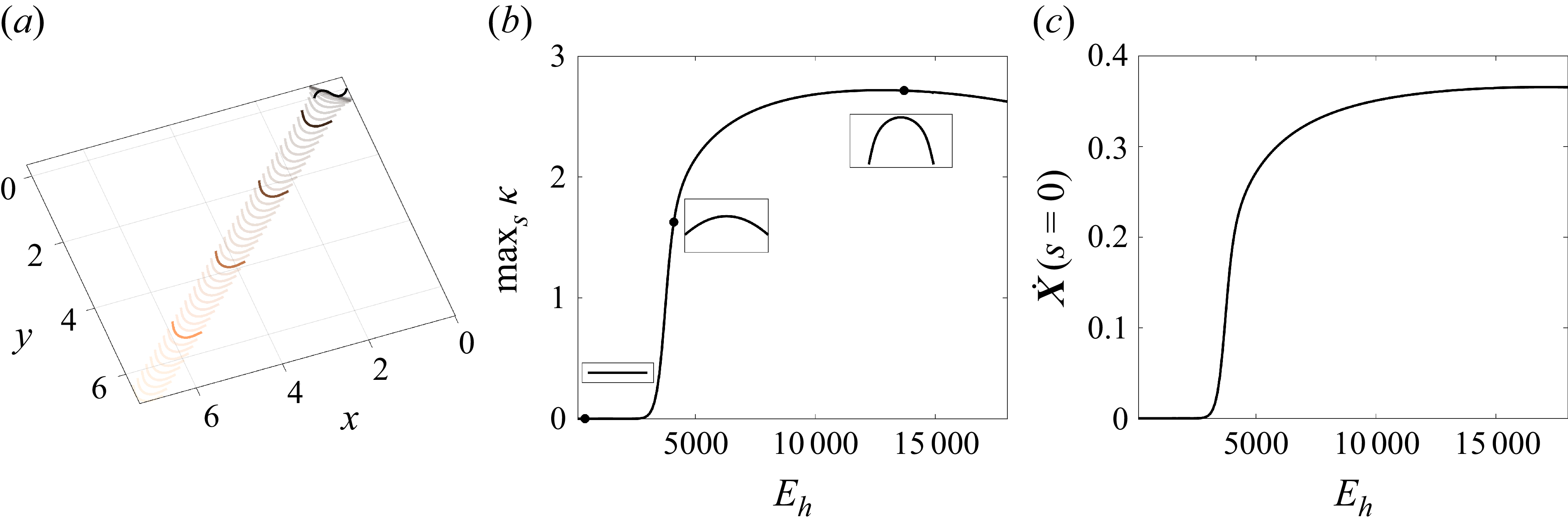


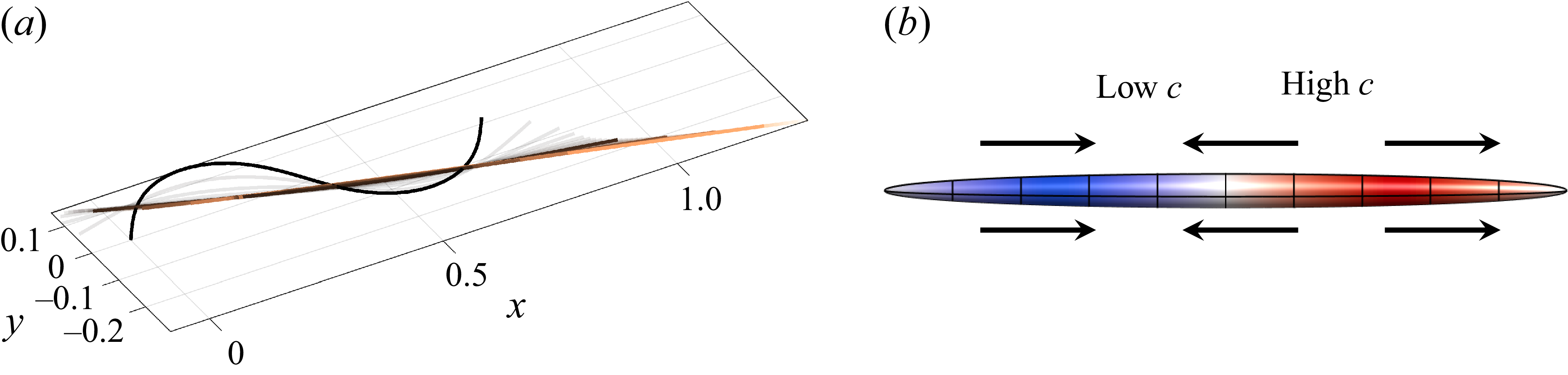


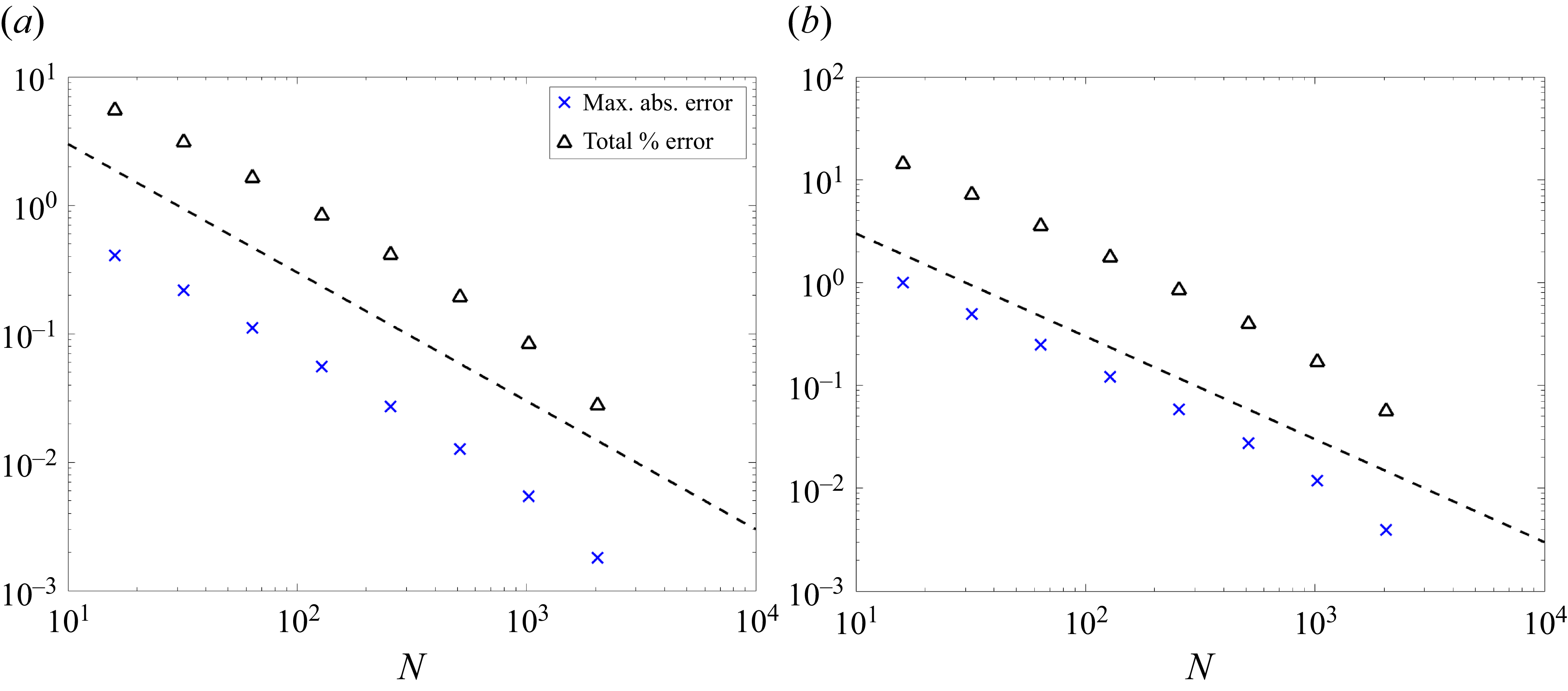


 Open access