


1. Introduction
It is well known that one of the most important properties of incompressible wall-bounded turbulence is the law of the wall, where the mean streamwise velocity exhibits a logarithmic scaling when normalised by the friction velocity. This canonical profile, typically expressed as
 \begin{equation} U^+ = \frac {1}{\kappa } \log \left (y^+\right ) + B, \end{equation}
has been a cornerstone in the development of turbulence modelling. Here, $U^{+}=\bar{u}/u_\tau$
is the non-dimensional mean streamwise velocity,
$U^{+}=\bar{u}/u_\tau$
is the non-dimensional mean streamwise velocity, $\bar{u}$
is the mean streamwise velocity,
$\bar{u}$
is the mean streamwise velocity, $ u_\tau =\sqrt {\bar {\tau }_w/\bar {\rho }_w}$
is the friction velocity,
$ u_\tau =\sqrt {\bar {\tau }_w/\bar {\rho }_w}$
is the friction velocity, $\bar {\tau }_w$
is the mean wall shear stress, and
$\bar {\tau }_w$
is the mean wall shear stress, and $\bar {\rho }_w$
is the mean wall density. Additionally,
$\bar {\rho }_w$
is the mean wall density. Additionally, $y^+=y/\delta _{\nu }$
is the non-dimensional wall-normal coordinate, where
$y^+=y/\delta _{\nu }$
is the non-dimensional wall-normal coordinate, where $\delta _{\nu }=\bar {\nu }_{w}/u_{\tau }$
is the viscous length scale,
$\delta _{\nu }=\bar {\nu }_{w}/u_{\tau }$
is the viscous length scale, $\bar {\nu }_{w}=\bar {\mu }_{w}/\bar {\rho }_w$
is the kinematic viscosity at the wall,
$\bar {\nu }_{w}=\bar {\mu }_{w}/\bar {\rho }_w$
is the kinematic viscosity at the wall, $\bar {\mu }_w$
is the dynamic viscosity at the wall, and
$\bar {\mu }_w$
is the dynamic viscosity at the wall, and $\bar {\phi }$
denotes Reynolds-averaged statistics. Also,
$\bar {\phi }$
denotes Reynolds-averaged statistics. Also, $\kappa$
is the von Kármán constant and
$\kappa$
is the von Kármán constant and $B$
is an integration constant. Inspired by the Reynolds analogy, which posits that momentum and heat transfer share similar turbulent transport mechanisms, a logarithmic scaling for the mean temperature in low-speed turbulent boundary layers has also been discovered (Kader Reference Kader1981), taking the form
$B$
is an integration constant. Inspired by the Reynolds analogy, which posits that momentum and heat transfer share similar turbulent transport mechanisms, a logarithmic scaling for the mean temperature in low-speed turbulent boundary layers has also been discovered (Kader Reference Kader1981), taking the form
 \begin{equation} \frac {\bar {\theta }}{\theta _{\tau }} = \frac {1}{\kappa _T} \log \left (y^+\right ) + B_T, \end{equation}
where $\bar {\theta } = \overline {T}{-} \overline {T}_w$
represents the difference between the mean temperature
$\bar {\theta } = \overline {T}{-} \overline {T}_w$
represents the difference between the mean temperature $\overline{T}$
and mean wall temperature
$\overline{T}$
and mean wall temperature $\overline{T}_w$
,
$\overline{T}_w$
, $\theta _{\tau } = \bar {q}_w / (\bar {\rho }_w c_p u_{\tau })$
is the friction temperature,
$\theta _{\tau } = \bar {q}_w / (\bar {\rho }_w c_p u_{\tau })$
is the friction temperature, $\bar{q}_w$
is the heat flux on the wall and
$\bar{q}_w$
is the heat flux on the wall and $c_p$
denotes the specific heat at constant pressure,
$c_p$
denotes the specific heat at constant pressure, $\kappa _T$
and
$\kappa _T$
and $B_T$
serve as analogous counterparts to the constants
$B_T$
serve as analogous counterparts to the constants $\kappa$
and
$\kappa$
and $B$
, with their values typically governed by the Prandtl number
$B$
, with their values typically governed by the Prandtl number $ \textit{Pr} $
.
$ \textit{Pr} $
.
For compressible turbulent flows, particularly at high Mach numbers, the situation is significantly more complex due to compressibility effects and aerodynamic heating. Following Morkovin’s hypothesis, which suggests that compressible turbulence dynamics can be mapped to incompressible flows by accounting for variations in fluid properties, numerous studies have developed transformations to map the compressible mean velocity profiles to their incompressible counterparts and recover the law of the wall. Notable examples include the transformations proposed by van Driest (Reference van Driest1951), Zhang et al (Reference Zhang, Bi, Hussain, Li and She2012), Trettel & Larsson (Reference Trettel and Larsson2016), Griffin, Fu & Moin (Reference Griffin, Fu and Moin2021), which account for compressibility effects and have significantly advanced turbulence modelling in high-speed flows.
In contrast, the extension to temperature transformations for compressible turbulent flows has been relatively underexplored due to the challenges posed by the complex coupling between velocity, pressure and temperature fields, alongside the influence of distinct wall thermal boundary conditions. Although algebraic temperature–velocity relations, such as the Crocco–Busemann formula and its modified versions (Walz Reference Walz1969; Duan & Martin Reference Duan and Martin2011; Zhang et al Reference Zhang, Bi, Hussain and She2014), have been proposed to connect the mean velocity and temperature in compressible flows, the corresponding implementation for modelling purposes typically necessitates the velocity and temperature values at the boundary-layer edge. However, the determination of boundary-layer thickness for complex flows is non-trivial and additional methodologies must be devised to estimate the values at the boundary-layer edge, which increases the complexity of the modelling process. Hence, direct temperature transformations within the inner layer are more desirable for the development of near-wall models in compressible wall turbulence.
A straightforward method for constructing a temperature transformation leverages the methodology of van Driest velocity transformations (van Driest Reference van Driest1951). Besides this, Patel, Boersma & Pecnik (Reference Patel, Boersma and Pecnik2017) develop an invariant function for the mean scalar field in variable-property turbulent channel flows at low Mach numbers and propose a semi-local-type temperature transformation, which effectively collapses the temperature profile under the non-adiabatic wall condition. However, the neglect of aerodynamic heating effects significantly constrains its applicability to high-speed compressible flows. Furthermore, observing that classical temperature normalisation based on the friction temperature becomes singular under adiabatic wall boundary conditions, where wall heat flux is zero, Chen et al (Reference Chen, Huang, Shi, Yang and Lv2022a ) introduce corrected van Driest and semi-local-type temperature transformations. By utilising local heat flux instead of wall heat flux, these temperature transformations are applicable to both isothermal and adiabatic wall conditions. More recently, Cheng & Fu (Reference Cheng and Fu2024) propose another van-Driest-type temperature transformation through the employment of semi-local scaling to diminish the Mach-number effects, which demonstrates improved performance in channel flows with adiabatic walls.
However, existing temperature transformations are typically designed and validated for supersonic channel and Couette flows, characterised by monotonic temperature profiles in the wall-normal direction. For supersonic and hypersonic turbulent boundary layers with cold walls, strong compressibility and aerodynamic heating effects induce pronounced non-monotonic temperature distributions in the wall-normal direction, posing significant challenges to the development of effective temperature transformations. Against this backdrop, we introduce a composite temperature transformation tailored for compressible turbulent boundary layers in this study. This new transformation seeks to recover the mean temperature profiles in compressible turbulent boundary layers with various Mach numbers and wall thermal conditions into the incompressible reference data, thereby providing a more robust tool for the turbulence modelling in high-speed flows.
2. Conventional temperature transformations
Throughout this study, both the Reynolds- (denoted as $\bar {\phi }$
) and the Favre-averaged (denoted as
$\bar {\phi }$
) and the Favre-averaged (denoted as $\widetilde {\phi }=\overline {\rho \phi }/\overline {\rho }$
) statistics are employed. Here,
$\widetilde {\phi }=\overline {\rho \phi }/\overline {\rho }$
) statistics are employed. Here, $\overline{\rho}$
is the mean density. The corresponding fluctuating components are represented as
$\overline{\rho}$
is the mean density. The corresponding fluctuating components are represented as $\phi '$
and
$\phi '$
and $\phi ^{\prime\prime}$
, respectively. Wall quantities are denoted by the subscript
$\phi ^{\prime\prime}$
, respectively. Wall quantities are denoted by the subscript $w$
, whereas the superscripts
$w$
, whereas the superscripts $+$
and
$+$
and $*$
indicate the wall scaling and semi-local scaling, respectively.
$*$
indicate the wall scaling and semi-local scaling, respectively.
2.1. Semi-local-type temperature transformation
Considering the statistically steady boundary-layer flows, the two-dimensional compressible energy equation can be cast as (Cebeci Reference Cebeci1974; Younes Reference Younes2021; Cheng & Fu Reference Cheng and Fu2024)
 \begin{align} \frac {\partial (\bar {\rho } \tilde {H} \tilde {u})}{\partial x} +\frac {\partial (\bar {\rho } \tilde {H} \tilde {v})}{\partial y}= &\frac {\partial }{\partial x}\left (\bar {q}_x-\overline {\rho H^{\prime \prime } u^{\prime \prime }}+\overline {u \tau _{x x}}+\overline {v \tau _{y x}}\right )\\ \nonumber&\quad + \frac {\partial }{\partial y}\left (\bar {q}_y-\overline {\rho H^{\prime \prime } v^{\prime \prime }}+\overline {u \tau _{x y}}+\overline {v \tau _{y y}}\right ), \end{align}
where $H=c_pT+(1/2)u^2$
denotes the total enthalpy;
$H=c_pT+(1/2)u^2$
denotes the total enthalpy; ${T}$
is the instantaneous temperature;
${T}$
is the instantaneous temperature; $\bar{q}_x$
is the streamwise heat flux;
$\bar{q}_x$
is the streamwise heat flux; $\boldsymbol{\tau}_{ij}$
and
$\boldsymbol{\tau}_{ij}$
and $\bar {q}_y=c_p({\bar {\mu }}/{Pr})({\partial \bar {\theta }}/{\partial y}) $
are the viscous stress tensor and the wall-normal heat flux, respectively;
$\bar {q}_y=c_p({\bar {\mu }}/{Pr})({\partial \bar {\theta }}/{\partial y}) $
are the viscous stress tensor and the wall-normal heat flux, respectively; $\bar{\mu}$
denotes the mean dynamic viscosity;
$\bar{\mu}$
denotes the mean dynamic viscosity; $u$
and
$u$
and $v$
represent the instantaneous streamwise and wall-normal velocities, respectively. Following the boundary-layer approximation and the scaling analysis of the energy terms, (2.1) can be further simplified into
$v$
represent the instantaneous streamwise and wall-normal velocities, respectively. Following the boundary-layer approximation and the scaling analysis of the energy terms, (2.1) can be further simplified into
 \begin{equation} \frac {\partial }{\partial y}\left (\bar {q}_y-\overline {\rho H^{\prime \prime } v^{\prime \prime }}+\overline {u \tau _{x y}}\right )=0. \end{equation}
The details are reported in Appendix A. It is pertinent to note that Younes (Reference Younes2021) has meticulously investigated this simplification process, allowing for a concise overview here. For a comprehensive understanding of the derivation, readers are directed to consult the foundational works of Cebeci (Reference Cebeci1974) and Younes (Reference Younes2021). The integration of (2.2) along the whole boundary layer results in
 \begin{equation} \bar {q}_y-\overline {\rho H^{\prime \prime } v^{\prime \prime }}+\overline {u \tau _{x y}}=Q, \end{equation}
where $ Q$
is the constant of integration, which can be evaluated by applying the boundary condition at the wall:
$ Q$
is the constant of integration, which can be evaluated by applying the boundary condition at the wall:
 \begin{equation} \underbrace {{{\left . \bar {q}_y \right |}_{y = 0}}}_{\bar q_w}- \underbrace {{{\left . {\overline {\rho {H^{\prime \prime }}{v^{\prime \prime }}} } \right |}_{y = 0}}}_0 + \underbrace {{{\left . {\overline {u{\tau _{xy}}} } \right |}_{y = 0}}}_0 = {\bar q_w} = Q. \end{equation}
Considering the definition of total enthalpy and the constant specific heat assumption, the corresponding fluctuating component $ H^{\prime \prime }$
can be derived as
$ H^{\prime \prime }$
can be derived as
 \begin{equation} H^{\prime \prime }=c_pT^{\prime \prime }+\frac {1}{2}u^{\prime \prime 2}+\tilde {u}u^{\prime \prime }. \end{equation}
Substituting (2.5) and (2.4) into (2.3) gives
 \begin{equation} \bar {q}_y-c_p\overline {\rho v^{\prime \prime } T^{\prime \prime }}={\bar q_w}+\overline {\rho \frac {1}{2}u^{\prime \prime 2}v^{\prime \prime }}+\overline {\rho \tilde {u}u^{\prime \prime }v^{\prime \prime }}-\overline {u \tau _{x y}}. \end{equation}
By retaining only the leading terms and invoking the constant-stress-layer approximation, the third and fourth terms on the right-hand side of (2.6) can be approximated as
 \begin{equation} \overline {\rho \tilde {u}u^{\prime\prime}v^{\prime \prime }}-\overline {u \tau _{x y}} \approx \tilde {u}\overline {\rho u^{\prime\prime}v^{\prime \prime }}-\tilde {u}\bar {\mu }\frac {\partial \tilde {u}}{\partial y} \approx -\tilde {u}\bar {\tau }_w. \end{equation}
Notably, the second term on the right-hand side of (2.6), representing a third-order correlation, is deemed negligible relative to other terms. To validate the rationality, we evaluate the magnitude of each term on the right-hand side of (2.6), as depicted in figure 1. It can be seen that $\overline {u \tau _{xy}}$
predominates in the near-wall region, whereas
$\overline {u \tau _{xy}}$
predominates in the near-wall region, whereas $\overline {\rho \tilde {u} u^{\prime \prime } v^{\prime \prime }}$
prevails in the logarithmic region. In contrast, the third-order correlation
$\overline {\rho \tilde {u} u^{\prime \prime } v^{\prime \prime }}$
prevails in the logarithmic region. In contrast, the third-order correlation $\overline {\rho (1/2) u^{\prime \prime 2} v^{\prime \prime }}$
is found to be of negligible magnitude in both regions. Additionally, the ratio between
$\overline {\rho (1/2) u^{\prime \prime 2} v^{\prime \prime }}$
is found to be of negligible magnitude in both regions. Additionally, the ratio between $\overline {\rho (1/2)u^{\prime \prime 2}v^{\prime \prime }}$
and
$\overline {\rho (1/2)u^{\prime \prime 2}v^{\prime \prime }}$
and $ \overline {\rho \tilde {u}u^{\prime \prime }v^{\prime \prime }}{-}\overline {u \tau _{x y}}$
exhibits a relatively large value solely in the vicinity of
$ \overline {\rho \tilde {u}u^{\prime \prime }v^{\prime \prime }}{-}\overline {u \tau _{x y}}$
exhibits a relatively large value solely in the vicinity of $ y^* \approx 20$
, corresponding to the buffer region. It indicates that the third-order correlation term is only non-negligible within this limited range. Slightly rearranging (2.6) gives
$ y^* \approx 20$
, corresponding to the buffer region. It indicates that the third-order correlation term is only non-negligible within this limited range. Slightly rearranging (2.6) gives
 \begin{equation} \bar {q}_y-c_p\overline {\rho v^{\prime \prime } T^{\prime \prime }} \approx \bar {q}_w-\tilde {u}\bar {\tau }_w. \end{equation}
(a) Distributions of $ {\overline {u{\tau _{xy}}} ^ + }$
,
$ {\overline {u{\tau _{xy}}} ^ + }$
, $ {\overline {\rho \tilde u{u^{\prime \prime }}{v^{\prime \prime }}} ^ + }$
and
$ {\overline {\rho \tilde u{u^{\prime \prime }}{v^{\prime \prime }}} ^ + }$
and ${\overline {\rho (1/2)u^{\prime \prime 2}v^{\prime \prime }}}^ +$
for M6Tw076R5, M8Tw048R5 and M14Tw018R6 turbulent boundary-layer cases; (b) distributions of the ratio between
${\overline {\rho (1/2)u^{\prime \prime 2}v^{\prime \prime }}}^ +$
for M6Tw076R5, M8Tw048R5 and M14Tw018R6 turbulent boundary-layer cases; (b) distributions of the ratio between $\overline {\rho (1/2)u^{\prime \prime 2}v^{\prime \prime }}$
and
$\overline {\rho (1/2)u^{\prime \prime 2}v^{\prime \prime }}$
and $ \overline {\rho \tilde {u}u^{\prime \prime }v^{\prime \prime }}{-}\overline {u \tau _{x y}}$
. The specific parameters and data sources for these cases are provided in table 1.
$ \overline {\rho \tilde {u}u^{\prime \prime }v^{\prime \prime }}{-}\overline {u \tau _{x y}}$
. The specific parameters and data sources for these cases are provided in table 1.

With the introduction of the turbulent eddy conductivity $\alpha _t=-\overline {\rho v^{\prime\prime} T^{\prime\prime}}/( {\partial \bar {\theta }}/{\partial y})$
and the semi-local friction Reynolds number as
$\alpha _t=-\overline {\rho v^{\prime\prime} T^{\prime\prime}}/( {\partial \bar {\theta }}/{\partial y})$
and the semi-local friction Reynolds number as $R e_{\tau }^{*}=R e_{\tau } \sqrt { (\bar {\rho } / \bar {\rho }_{w} )} / (\bar {\mu } / \bar {\mu }_{w} )$
, (2.8) can be reformulated as
$R e_{\tau }^{*}=R e_{\tau } \sqrt { (\bar {\rho } / \bar {\rho }_{w} )} / (\bar {\mu } / \bar {\mu }_{w} )$
, (2.8) can be reformulated as
 \begin{equation} \underbrace {\left (\frac {\alpha _t}{\bar {\mu }}+\frac {1}{\textit{Pr}}\right )}_{\psi _1}\underbrace {\frac {\delta }{R e_{\tau }^{*}}\sqrt {\bar {\rho }^{+}}\frac {\partial \bar {\theta }^+}{\partial y}}_{\psi _2}\approx \underbrace {1-\frac {\tilde {u}\bar {\tau }_w}{\bar {q}_w}}_{\psi _3}, \end{equation}
where $\delta$
denotes the boundary-layer thickness. According to Chen et al (Reference Chen, Huang, Shi, Yang and Lv2022a
,
Reference Chen, Lv, Xu, Shi and Yangb
), the function
$\delta$
denotes the boundary-layer thickness. According to Chen et al (Reference Chen, Huang, Shi, Yang and Lv2022a
,
Reference Chen, Lv, Xu, Shi and Yangb
), the function $\psi _3$
exhibits a proportional relationship with the local heat flux in high-speed flows and is disregarded by Patel et al (Reference Patel, Boersma and Pecnik2017), since their analysis is grounded in direct numerical simulation (DNS) datasets of fully developed channel flows at low Mach numbers. Based on this low-Mach-number DNS dataset, Patel et al (Reference Patel, Boersma and Pecnik2017) demonstrated that, for a given Prandtl number,
$\psi _3$
exhibits a proportional relationship with the local heat flux in high-speed flows and is disregarded by Patel et al (Reference Patel, Boersma and Pecnik2017), since their analysis is grounded in direct numerical simulation (DNS) datasets of fully developed channel flows at low Mach numbers. Based on this low-Mach-number DNS dataset, Patel et al (Reference Patel, Boersma and Pecnik2017) demonstrated that, for a given Prandtl number, $\psi _2$
is a Mach-number invariant function with respect to
$\psi _2$
is a Mach-number invariant function with respect to $y^*$
. This finding further implies that the function
$y^*$
. This finding further implies that the function $\psi _1(y^*)$
is also independent of the flow property.
$\psi _1(y^*)$
is also independent of the flow property.
Parameters of the DNS datasets for turbulent boundary layers with adiabatic and heated walls (Nos $1{-}8$
), supersonic turbulent boundary layers with cold walls (Nos
$1{-}8$
), supersonic turbulent boundary layers with cold walls (Nos $9{-}17$
) and hypersonic turbulent boundary layers with cold walls (Nos
$9{-}17$
) and hypersonic turbulent boundary layers with cold walls (Nos $18{-}26$
). Here,
$18{-}26$
). Here, $Re_{\theta }$
and
$Re_{\theta }$
and $Re_{\tau }$
are the momentum-thickness-based Reynolds number and friction Reynolds number, respectively. Here,
$Re_{\tau }$
are the momentum-thickness-based Reynolds number and friction Reynolds number, respectively. Here, $\varTheta =(\bar {T}_w-T_e)/(\bar {T}_r-T_e)$
denotes the diabatic parameter;
$\varTheta =(\bar {T}_w-T_e)/(\bar {T}_r-T_e)$
denotes the diabatic parameter; $ \bar {T}_r$
and
$ \bar {T}_r$
and $ T_e$
are the recovery temperature and the temperature at the boundary-layer edge, respectively. The abbreviations for data sources are CBCBP for Cogo et al (Reference Cogo, Baù, Chinappi, Bernardini and Picano2023), VBL for Volpiani et al (Reference Volpiani, Bernardini and Larsson2018, Reference Volpiani, Bernardini and Larsson2020), ZDC for Zhang, Duan & Choudhari (Reference Zhang, Duan and Choudhari2018), CSPB for Cogo et al (Reference Cogo, Salvadore, Picano and Bernardini2022). The notation expresses the free stream Mach number
$ T_e$
are the recovery temperature and the temperature at the boundary-layer edge, respectively. The abbreviations for data sources are CBCBP for Cogo et al (Reference Cogo, Baù, Chinappi, Bernardini and Picano2023), VBL for Volpiani et al (Reference Volpiani, Bernardini and Larsson2018, Reference Volpiani, Bernardini and Larsson2020), ZDC for Zhang, Duan & Choudhari (Reference Zhang, Duan and Choudhari2018), CSPB for Cogo et al (Reference Cogo, Salvadore, Picano and Bernardini2022). The notation expresses the free stream Mach number $Ma_{\infty }$
,
$Ma_{\infty }$
, $\bar {T}_w/\bar {T}_r$
and
$\bar {T}_w/\bar {T}_r$
and $Re_{\tau }$
.
$Re_{\tau }$
.

However, the invariant function $\psi _2(y^*)$
proves inadequate for high-speed turbulent flows with adiabatic wall condition, as the absence of wall heat flux introduces singularities in the associated temperature transformations. To address the effects of aerodynamic heating while preserving the invariance of
$\psi _2(y^*)$
proves inadequate for high-speed turbulent flows with adiabatic wall condition, as the absence of wall heat flux introduces singularities in the associated temperature transformations. To address the effects of aerodynamic heating while preserving the invariance of $\psi _1(y^*)$
, it can be posited that the function
$\psi _1(y^*)$
, it can be posited that the function
 \begin{equation} \phi _{\textit{SL}}(y^*)=\dfrac {\dfrac {\delta }{R e_{\tau }^{*}}\sqrt {\bar {\rho }^{+}}\dfrac {\partial \bar {\theta }^+}{\partial y}}{1-\dfrac {\tilde {u}\bar {\tau }_w}{\bar {q}_w}}=\dfrac {\sqrt {\bar {\rho }^{+}}\bar {\rho }_w c_pu_{\tau }}{\bar {q}_w-\tilde {u}\bar {\tau }_w}\dfrac {\delta }{R e_{\tau }^{*}}\dfrac {\partial \bar {\theta }}{\partial y}=\dfrac {{c_p\bar {\mu }}}{{{\bar q}_w} - \tilde u{{\bar \tau }_w}}\dfrac {\partial \bar {\theta }}{\partial y} \end{equation}
is Mach number and wall temperature invariant. Integrating $\phi _{\textit{SL}}$
with respect to
$\phi _{\textit{SL}}$
with respect to $y^*$
yields the corrected semi-local-type transformation put forward by Chen et al (Reference Chen, Huang, Shi, Yang and Lv2022a
) (denoted as
$y^*$
yields the corrected semi-local-type transformation put forward by Chen et al (Reference Chen, Huang, Shi, Yang and Lv2022a
) (denoted as $\theta _{\textit{SL}}^+$
hereafter). It is noteworthy that, while the derivation process presented in this study exhibits minor differences from that articulated in Chen et al (Reference Chen, Huang, Shi, Yang and Lv2022a
), the final transformations are fundamentally equivalent.
$\theta _{\textit{SL}}^+$
hereafter). It is noteworthy that, while the derivation process presented in this study exhibits minor differences from that articulated in Chen et al (Reference Chen, Huang, Shi, Yang and Lv2022a
), the final transformations are fundamentally equivalent.
2.2. van-Driest-type temperature transformation
On the other hand, by analogy with the invariant function governing the mean velocity transformation in compressible wall turbulence, as originally proposed by van Driest (Reference van Driest1951), a similar Mach-number invariant function can be constructed as
 \begin{equation} \phi _{vD}(y^+)=\dfrac {\sqrt {\bar {\rho }^{+}}\dfrac {\partial \bar {\theta }^+}{\partial y^+}}{1-\dfrac {\tilde {u}\bar {\tau }_w}{\bar {q}_w}} =\dfrac {\sqrt {\bar {\rho }^{+}}\bar {\rho }_w c_pu_{\tau }}{\bar {q}_w-\tilde {u}\bar {\tau }_w}\dfrac {\partial \bar {\theta }}{\partial y^+}. \end{equation}
Integrating $\phi _{vD}$
with respect to
$\phi _{vD}$
with respect to $y^+$
yields the van-Driest-type temperature transformation put forward by Patel et al (Reference Patel, Boersma and Pecnik2017) and Chen et al (Reference Chen, Huang, Shi, Yang and Lv2022a
). However, in the context of supersonic and hypersonic turbulent boundary layers,
$y^+$
yields the van-Driest-type temperature transformation put forward by Patel et al (Reference Patel, Boersma and Pecnik2017) and Chen et al (Reference Chen, Huang, Shi, Yang and Lv2022a
). However, in the context of supersonic and hypersonic turbulent boundary layers, $\phi _{vD}(y^+)$
is reported to be less effective than the semi-local-type
$\phi _{vD}(y^+)$
is reported to be less effective than the semi-local-type $\phi _{\textit{SL}}(y^*)$
. To improve the performance, Cheng & Fu (Reference Cheng and Fu2024) propose another improved van-Driest-type Mach-number invariant function for the mean temperature field, which takes the form
$\phi _{\textit{SL}}(y^*)$
. To improve the performance, Cheng & Fu (Reference Cheng and Fu2024) propose another improved van-Driest-type Mach-number invariant function for the mean temperature field, which takes the form
 \begin{equation} \phi _{S}(y^*)=\dfrac {\sqrt {\bar {\rho }^{+}}\dfrac {\partial \bar {\theta }^+}{\partial y^*}}{1-\dfrac {\tilde {u}\bar {\tau }_w}{\bar {q}_w}}=\dfrac {\sqrt {\bar {\rho }^{+}}\bar {\rho }_w c_pu_{\tau }}{\bar {q}_w-\tilde {u}\bar {\tau }_w}\dfrac {\partial \bar {\theta }}{\partial y^*}. \end{equation}
Compared with $\phi _{vD}(y^+)$
, the semi-local wall-normal coordinate
$\phi _{vD}(y^+)$
, the semi-local wall-normal coordinate $y^*$
is employed as a more appropriate non-dimensionalisation approach to account for the mean property variation. Integrating
$y^*$
is employed as a more appropriate non-dimensionalisation approach to account for the mean property variation. Integrating $\phi _{S}$
with respect to
$\phi _{S}$
with respect to $y^*$
yields the improved van-Driest-type temperature transformation (denoted as
$y^*$
yields the improved van-Driest-type temperature transformation (denoted as $\theta _{S}^+$
hereafter).
$\theta _{S}^+$
hereafter).
3. A composite temperature transformation
To the best of the authors’ knowledge, the transformations proposed by Patel et al (Reference Patel, Boersma and Pecnik2017), Chen et al (Reference Chen, Huang, Shi, Yang and Lv2022a
) and Cheng & Fu (Reference Cheng and Fu2024) represent the latest advancements in temperature scaling for compressible turbulent flows. Although the semi-local-type and van-Driest-type transformations have achieved significant progress in flows with monotonic temperature profiles, such as channel and Couette flows, the overall effectiveness for compressible turbulent boundary layers remains unsatisfactory, especially for cold-wall cases characterised by the non-monotonicity of $ \bar {T}(y)$
. The critical challenge arises from the derivation of the Mach-number invariant functions, as both the numerator and denominator in (2.12) (also (2.11) and (2.10)) can be zero in proximity to the temperature peak where
$ \bar {T}(y)$
. The critical challenge arises from the derivation of the Mach-number invariant functions, as both the numerator and denominator in (2.12) (also (2.11) and (2.10)) can be zero in proximity to the temperature peak where $ {\partial \bar {T}(y)}/{\partial y} \approx 0$
. However, due to the unavoidable omission of numerous high-order fluctuating terms during the average process, the zero-crossing points of the numerator and denominator do not align at the same wall-normal location, causing the corresponding Mach-invariant function to become ill-defined or exhibit singular behaviour.
$ {\partial \bar {T}(y)}/{\partial y} \approx 0$
. However, due to the unavoidable omission of numerous high-order fluctuating terms during the average process, the zero-crossing points of the numerator and denominator do not align at the same wall-normal location, causing the corresponding Mach-invariant function to become ill-defined or exhibit singular behaviour.
To address this challenge and trigger advanced near-wall models, a novel temperature transformation is proposed in this study. First, unlike the existing methodologies that utilised the local heat transfer (represented by $ \bar {q}_w{-}\tilde {u}\bar {\tau }_w$
(Chen et al Reference Chen, Huang, Shi, Yang and Lv2022a
)) for scaling, we introduce an alternative approach by adopting the total heat flux (represented by
$ \bar {q}_w{-}\tilde {u}\bar {\tau }_w$
(Chen et al Reference Chen, Huang, Shi, Yang and Lv2022a
)) for scaling, we introduce an alternative approach by adopting the total heat flux (represented by $ \bar {q}_y{-}c_p\overline {\rho v^{\prime \prime } T^{\prime \prime }}$
) as the new temperature scale. Although these two quantities exhibit comparable values and dimensional consistency, as delineated in (2.8), numerical experiments employing multiple DNS datasets reveal that the total-heat-flux-based approach yields better scaling performance for the temperature field within the near-wall viscous sublayer, as depicted in figure 2. Notwithstanding this, the incorporation of additional turbulent fluctuation statistics represents a notable limitation, as most of existing open-source datasets lack these high-order statistics, thereby hindering in-depth investigations of their relationship with the mean temperature.
$ \bar {q}_y{-}c_p\overline {\rho v^{\prime \prime } T^{\prime \prime }}$
) as the new temperature scale. Although these two quantities exhibit comparable values and dimensional consistency, as delineated in (2.8), numerical experiments employing multiple DNS datasets reveal that the total-heat-flux-based approach yields better scaling performance for the temperature field within the near-wall viscous sublayer, as depicted in figure 2. Notwithstanding this, the incorporation of additional turbulent fluctuation statistics represents a notable limitation, as most of existing open-source datasets lack these high-order statistics, thereby hindering in-depth investigations of their relationship with the mean temperature.
Premultiplied non-dimensionalisations of the mean temperature shear based on the local heat transfer $ \bar {q}_w{-}\tilde {u}\bar {\tau }_w$
and the total heat flux
$ \bar {q}_w{-}\tilde {u}\bar {\tau }_w$
and the total heat flux $ \bar {q}_y-c_p\overline {\rho v^{\prime \prime } T^{\prime \prime }}$
for (a) M6Tw076R5, (b) M8Tw048R5 and (c) M14Tw018R6 turbulent boundary-layer cases. The specific parameters and data sources for these cases are provided in table 1.
$ \bar {q}_y-c_p\overline {\rho v^{\prime \prime } T^{\prime \prime }}$
for (a) M6Tw076R5, (b) M8Tw048R5 and (c) M14Tw018R6 turbulent boundary-layer cases. The specific parameters and data sources for these cases are provided in table 1.

To further maintain the conciseness of the scaling, a variable turbulent heat flux model
 \begin{equation} \bar {q}_t=-{{{c_p}\overline {\rho v^{\prime \prime }T^{\prime \prime }} }} \approx \dfrac {{-\overline {\rho {u^{\prime \prime }}v^{\prime \prime }} }}{{{{\bar \tau }_w}}}({{{{\bar q}_w} - \tilde u{{\bar \tau }_w}}}) \approx \dfrac {{ {{\bar \tau }_w}-\bar {\mu }\dfrac {\partial \tilde {u}}{\partial y}}}{{{{\bar \tau }_w}}} ({{\bar q}_w} - \tilde u{{\bar \tau }_w}) \end{equation}
is introduced by analogy with the turbulent Reynolds stress in the velocity field. The motivation for this heuristic model arises from the pronounced correlation and coherence between streamwise velocity fluctuations and temperature fluctuations within the viscous sublayer, where these fluctuations are driven primarily by coherent near-wall velocity and temperature streaks (Cogo et al Reference Cogo, Salvadore, Picano and Bernardini2022; Cheng & Fu Reference Cheng and Fu2023). This strong correlation provides a robust physical foundation for using the turbulent Reynolds stress $\overline {\rho u^{\prime \prime } v^{\prime \prime }}$
to approximate the turbulent heat flux
$\overline {\rho u^{\prime \prime } v^{\prime \prime }}$
to approximate the turbulent heat flux $\overline {\rho v^{\prime \prime } T^{\prime \prime }}$
. Specifically, the term
$\overline {\rho v^{\prime \prime } T^{\prime \prime }}$
. Specifically, the term $(\bar {q}_w {-} \tilde {u} \bar {\tau }_w)$
, which encapsulates the combined effects of wall heat flux
$(\bar {q}_w {-} \tilde {u} \bar {\tau }_w)$
, which encapsulates the combined effects of wall heat flux $\bar{q}_w$
and wall-distance-dependent viscous heating, serves as an approximation for the local heat transfer, such that
$\bar{q}_w$
and wall-distance-dependent viscous heating, serves as an approximation for the local heat transfer, such that $(\bar {q}_w - \tilde {u} \bar {\tau }_w) \approx c_p ( {\bar {\mu }}/{\textit{Pr}})( {\partial \bar {T}}/{\partial y}) $
(Chen et al Reference Chen, Huang, Shi, Yang and Lv2022a
; Bradshaw & Huang Reference Bradshaw and Huang1995). Similarly, in the near-wall region, the wall shear stress
$(\bar {q}_w - \tilde {u} \bar {\tau }_w) \approx c_p ( {\bar {\mu }}/{\textit{Pr}})( {\partial \bar {T}}/{\partial y}) $
(Chen et al Reference Chen, Huang, Shi, Yang and Lv2022a
; Bradshaw & Huang Reference Bradshaw and Huang1995). Similarly, in the near-wall region, the wall shear stress ${\bar\tau}_w$
provides a coarse approximation for the local shear stress, i.e.
${\bar\tau}_w$
provides a coarse approximation for the local shear stress, i.e. ${\bar\tau}_w \approx \bar {\mu } ( {\partial \bar{u}}/{\partial y})$
. Consequently, (3.1) posits that the turbulent Reynolds stress, when normalised by the local shear stress, is proportional to the turbulent heat flux normalised by the local heat transfer. Alternatively, from a conceptual standpoint, (3.1) can be interpreted as a variant of
${\bar\tau}_w \approx \bar {\mu } ( {\partial \bar{u}}/{\partial y})$
. Consequently, (3.1) posits that the turbulent Reynolds stress, when normalised by the local shear stress, is proportional to the turbulent heat flux normalised by the local heat transfer. Alternatively, from a conceptual standpoint, (3.1) can be interpreted as a variant of $\textit{Pr}_t = ({\overline {\rho u^{\prime \prime } v^{\prime \prime }}}/{\overline {\rho v^{\prime \prime } T^{\prime \prime }}}) (\partial \bar{T} / \partial y)/(\partial \tilde{u} / \partial y)\approx \text{const}$
, which has been found to be insensitive to Mach number and wall-temperature conditions in the near-wall region across various studies (Zhang et al Reference Zhang, Bi, Hussain and She2014; Gibis et al Reference Gibis, Sciacovelli, Kloker and Wenzel2024). Nevertheless, it should be acknowledged that this heuristic model is expected to hold only within the viscous sublayer. In the buffer layer or the logarithmic region farther from the wall, the strong correlation between the streamwise velocity fluctuations and temperature fluctuations as well as the constant-stress-layer assumption become invalid and introduce substantial errors.
$\textit{Pr}_t = ({\overline {\rho u^{\prime \prime } v^{\prime \prime }}}/{\overline {\rho v^{\prime \prime } T^{\prime \prime }}}) (\partial \bar{T} / \partial y)/(\partial \tilde{u} / \partial y)\approx \text{const}$
, which has been found to be insensitive to Mach number and wall-temperature conditions in the near-wall region across various studies (Zhang et al Reference Zhang, Bi, Hussain and She2014; Gibis et al Reference Gibis, Sciacovelli, Kloker and Wenzel2024). Nevertheless, it should be acknowledged that this heuristic model is expected to hold only within the viscous sublayer. In the buffer layer or the logarithmic region farther from the wall, the strong correlation between the streamwise velocity fluctuations and temperature fluctuations as well as the constant-stress-layer assumption become invalid and introduce substantial errors.
To demonstrate the effectiveness within the viscous sublayer, figure 3 compares the normalised turbulent heat flux $\bar {q}_t^+=\bar {q}_t/{{\bar q}_w}$
derived from DNS data and the modelled turbulent heat flux with mean flow quantities
$\bar {q}_t^+=\bar {q}_t/{{\bar q}_w}$
derived from DNS data and the modelled turbulent heat flux with mean flow quantities $ \bar {q}_{t,m}^+=({{\bar \tau }_w}-{\bar {\mu }({\partial \tilde {u}}/{\partial y} }) )({({{\bar q}_w} - \tilde u{{\bar \tau }_w})}/{{{{\bar \tau }_w}}}) /{{\bar q}_w}$
. The small discrepancy between
$ \bar {q}_{t,m}^+=({{\bar \tau }_w}-{\bar {\mu }({\partial \tilde {u}}/{\partial y} }) )({({{\bar q}_w} - \tilde u{{\bar \tau }_w})}/{{{{\bar \tau }_w}}}) /{{\bar q}_w}$
. The small discrepancy between $ {\bar q}_t^+$
and
$ {\bar q}_t^+$
and $ {\bar q}_{t,m}^+$
in the near-wall viscous sublayer underscores the approximation’s reliability. Substituting (3.1) into (2.6), we obtain
$ {\bar q}_{t,m}^+$
in the near-wall viscous sublayer underscores the approximation’s reliability. Substituting (3.1) into (2.6), we obtain
 \begin{equation} \underbrace {\dfrac {{\bar q_w}+\overline {\rho \dfrac {1}{2}u^{\prime \prime 2}v^{\prime \prime }}+\overline {\rho \tilde {u}u^{\prime \prime }v^{\prime \prime }}-\overline {u \tau _{x y}}}{{\sqrt {\bar {\rho }^{+}}\bar {\rho }_w c_pu_{\tau }}\dfrac {\delta }{R e_{\tau }^{*}}\dfrac {\partial \bar {\theta }}{\partial y}}}_{\psi _4} {c_p\bar {\mu }\dfrac {\partial \bar {\theta }}{\partial y}} \approx \dfrac {c_p{\bar {\mu }}}{\textit{Pr}}\dfrac {\partial \bar {\theta }}{\partial y}-\dfrac {{\bar {\mu }\dfrac {\partial \tilde {u}}{\partial y} - {{\bar \tau }_w}}}{{{{\bar \tau }_w}}} ({{\bar q}_w} - \tilde u{{\bar \tau }_w}). \end{equation}
It can be analysed that the Mach-number invariant function $ \phi _{\textit{SL}}(y^*)$
can be regarded as the inverse of
$ \phi _{\textit{SL}}(y^*)$
can be regarded as the inverse of $ {\psi _4}$
when neglecting the high-order fluctuating terms. Given that the function
$ {\psi _4}$
when neglecting the high-order fluctuating terms. Given that the function $\phi _{\textit{SL}}(y^*)$
exhibits a substantial degree of independence from flow properties, it is straightforward to conjecture that the function
$\phi _{\textit{SL}}(y^*)$
exhibits a substantial degree of independence from flow properties, it is straightforward to conjecture that the function
 \begin{equation} \phi _{V}(y^*)=\dfrac {{c_p\bar {\mu }\dfrac {\partial \bar {\theta }}{\partial y}}}{\dfrac {c_p{\bar {\mu }}}{\textit{Pr}}\dfrac {\partial \bar {\theta }}{\partial y}-\dfrac {{\bar {\mu }\dfrac {\partial \tilde {u}}{\partial y} - {{\bar \tau }_w}}}{{{{\bar \tau }_w}}} ({{\bar q}_w} - \tilde u{{\bar \tau }_w})} \end{equation}
Distributions of $ \bar {q}^+$
,
$ \bar {q}^+$
, $\bar {q}_y^+$
,
$\bar {q}_y^+$
, $ \bar {q}_t^+$
and
$ \bar {q}_t^+$
and $ \bar {q}_{t,m}^+$
for (a) M6Tw076R5, (b) M8Tw048R5 and (c) M14Tw018R6 turbulent boundary-layer cases. The specific parameters and data sources for these cases are provided in table 1.
$ \bar {q}_{t,m}^+$
for (a) M6Tw076R5, (b) M8Tw048R5 and (c) M14Tw018R6 turbulent boundary-layer cases. The specific parameters and data sources for these cases are provided in table 1.

is also Mach number and wall temperature invariant with respect to $ y^*$
. To demonstrate the applicability, figure 4 shows the distributions of premultiplied mean temperature shear
$ y^*$
. To demonstrate the applicability, figure 4 shows the distributions of premultiplied mean temperature shear $y^*\phi _{\textit{SL}}$
,
$y^*\phi _{\textit{SL}}$
, $y^*\phi _{S}$
and present
$y^*\phi _{S}$
and present $y^*\phi _{V}$
in the viscous sublayer. In comparison with the classical Mach-number functions, the variation of
$y^*\phi _{V}$
in the viscous sublayer. In comparison with the classical Mach-number functions, the variation of $y^* \phi _{V}$
exhibits improved consistency with that of the incompressible reference data in the viscous sublayer. However, it should be recognised that both the total-heat-flux-based temperature scale and the approximation employed in (3.1) exhibit increasing deficiencies within the logarithmic region, as demonstrated in figure 3, resulting in a case-dependent behaviour of the function
$y^* \phi _{V}$
exhibits improved consistency with that of the incompressible reference data in the viscous sublayer. However, it should be recognised that both the total-heat-flux-based temperature scale and the approximation employed in (3.1) exhibit increasing deficiencies within the logarithmic region, as demonstrated in figure 3, resulting in a case-dependent behaviour of the function $ \phi _{V}(y^*)$
. To overcome this limitation and achieve a more general temperature scaling, we subsequently introduce a new Mach-number invariant function
$ \phi _{V}(y^*)$
. To overcome this limitation and achieve a more general temperature scaling, we subsequently introduce a new Mach-number invariant function
 \begin{equation} \phi _{L}(y^*)=\frac {\bar {\rho } c_pu_{\tau }}{\bar {q}_w-\tilde {u}\bar {\tau }_w}\frac {\delta }{R e_{\tau }^{*}}\frac {\partial \bar {\theta }}{\partial (y\sqrt {\bar {\rho }^{+}})}=\frac {{c_p\bar {\mu }\sqrt {\bar \rho ^{+}}}}{{{\bar q}_w} - \tilde u{{\bar \tau }_w}}\frac {\partial \bar {\theta }}{\partial (y\sqrt {\bar {\rho }^{+}})} \end{equation}
for the logarithmic region of turbulent boundary layers. Compared with the conventional function $ \phi _{\textit{SL}}(y^*)$
in (2.10), the van-Driest-type differentiation
$ \phi _{\textit{SL}}(y^*)$
in (2.10), the van-Driest-type differentiation $ \sqrt {\bar \rho ^{+}}\partial \bar {\theta }$
is retained in the new Mach-number invariant function to account for the density variation, facilitated by the introduction of the density-weighted wall-normal coordinate
$ \sqrt {\bar \rho ^{+}}\partial \bar {\theta }$
is retained in the new Mach-number invariant function to account for the density variation, facilitated by the introduction of the density-weighted wall-normal coordinate $ y\sqrt {\bar {\rho }^{+}}$
for dimensional consistency. Consequently,
$ y\sqrt {\bar {\rho }^{+}}$
for dimensional consistency. Consequently, $ \phi _{L}(y^*)$
is discovered to be more appropriate for mapping the wall-normal distributions of compressible temperature statistics to their incompressible counterparts in the logarithmic region, as evidenced in figure 5. Notwithstanding this, we want to acknowledge that the current choice relies chiefly on empirical numerical results rather than explicit physical insights; the underlying mechanisms and extension to other turbulence statistics merit future exploration.
$ \phi _{L}(y^*)$
is discovered to be more appropriate for mapping the wall-normal distributions of compressible temperature statistics to their incompressible counterparts in the logarithmic region, as evidenced in figure 5. Notwithstanding this, we want to acknowledge that the current choice relies chiefly on empirical numerical results rather than explicit physical insights; the underlying mechanisms and extension to other turbulence statistics merit future exploration.
Distributions of premultiplied mean temperature shear (a) $y^*\phi _{\textit{SL}}$
, (b)
$y^*\phi _{\textit{SL}}$
, (b) $y^*\phi _{S}$
and (c)
$y^*\phi _{S}$
and (c) $y^*\phi _{V}$
in the viscous sublayer for compressible turbulent boundary layers. The specific parameters and data sources for these cases are provided in table 1.
$y^*\phi _{V}$
in the viscous sublayer for compressible turbulent boundary layers. The specific parameters and data sources for these cases are provided in table 1.

Distributions of premultiplied mean temperature shear (a) $y^*\phi _{\textit{SL}}$
, (b)
$y^*\phi _{\textit{SL}}$
, (b) $y^*\phi _{S}$
and (c)
$y^*\phi _{S}$
and (c) $y^*\phi _{L}$
in the logarithmic region for compressible turbulent boundary layers. The specific parameters and data sources for these cases are provided in table 1.
$y^*\phi _{L}$
in the logarithmic region for compressible turbulent boundary layers. The specific parameters and data sources for these cases are provided in table 1.

Upon this discussion, it is sensible to derive a composite temperature transformation across the entire inner layer by leveraging different invariant functions in the viscous sublayer and the logarithmic region. Motivated by Griffin et al (Reference Griffin, Fu and Moin2021), a generalised non-dimensional temperature gradient $\phi _{\textit{VL}}$
can be defined as
$\phi _{\textit{VL}}$
can be defined as
 \begin{equation} \bar {q}=\phi _{\textit{VL}}\left (\frac {\bar {q}_{y}}{\phi _{V}}+\frac {\bar {q}_{t}}{\phi _{L}}\right )\!, \end{equation}
where $\bar {q}=\bar {q}_{y}+\bar {q}_{t}$
denotes the total heat flux generated by the fluid viscosity and turbulent transport. The blending in (3.5) is physically grounded in the dominance of viscous heat flux in the viscous sublayer, where turbulent transport is negligible, and turbulent heat flux in the logarithmic region, where molecular viscosity effects are minimal. As a sanity check, figure 3 compares the normalised total heat flux
$\bar {q}=\bar {q}_{y}+\bar {q}_{t}$
denotes the total heat flux generated by the fluid viscosity and turbulent transport. The blending in (3.5) is physically grounded in the dominance of viscous heat flux in the viscous sublayer, where turbulent transport is negligible, and turbulent heat flux in the logarithmic region, where molecular viscosity effects are minimal. As a sanity check, figure 3 compares the normalised total heat flux $ \bar {q}^+$
, viscous heat flux
$ \bar {q}^+$
, viscous heat flux $ \bar {q}_y^+$
, and turbulent heat flux
$ \bar {q}_y^+$
, and turbulent heat flux $ \bar {q}_t^+$
for three representative boundary-layer flows with varying Mach numbers and wall temperatures. It can be analysed that, in the near-wall viscous sublayer where
$ \bar {q}_t^+$
for three representative boundary-layer flows with varying Mach numbers and wall temperatures. It can be analysed that, in the near-wall viscous sublayer where $\bar {q} \rightarrow \bar {q}_{y}$
, the relation
$\bar {q} \rightarrow \bar {q}_{y}$
, the relation $\phi _{\textit{VL}} \rightarrow \phi _{V}$
can be established by this construction, whereas in the logarithmic region where
$\phi _{\textit{VL}} \rightarrow \phi _{V}$
can be established by this construction, whereas in the logarithmic region where $\bar {q} \rightarrow \bar {q}_{t}$
,
$\bar {q} \rightarrow \bar {q}_{t}$
, $\phi _{\textit{VL}}\rightarrow \phi _{L}$
holds. Observing that the derivation of
$\phi _{\textit{VL}}\rightarrow \phi _{L}$
holds. Observing that the derivation of $ \phi _{V}$
implies
$ \phi _{V}$
implies $\bar {q}_{y}/\bar {q} \approx \phi _{V}/\textit{Pr}$
, (3.5) can be further rearranged for
$\bar {q}_{y}/\bar {q} \approx \phi _{V}/\textit{Pr}$
, (3.5) can be further rearranged for $ \phi _{\textit{VL}}$
as
$ \phi _{\textit{VL}}$
as
 \begin{equation} {\phi _{\textit{VL}}} = \frac {{\bar q{\phi _V}{\phi _L}}}{{{{\bar q}_y}{\phi _L} + {{\bar q}_t}{\phi _V}}} = \frac {{{\phi _V}{\phi _L}}}{{{\phi _L}{{\bar q}_y}/\bar q + (1 - {{\bar q}_y}/\bar q){\phi _V}}} \approx \frac {{\textit{Pr}{\phi _L}}}{{{\phi _L} + \textit{Pr} - {\phi _V}}}. \end{equation}
Finally, the transformed temperature can be obtained by $\theta _{\textit{VL}}^+(y^*)=\int \phi _{\textit{VL}} dy^*$
. From a general view, it bears emphasis that this composite transformation not only deploys appropriate Mach-number invariant functions as the non-dimensional temperature gradient in the viscous sublayer and the logarithmic region, but also introduces an improved solution to the long-standing singularity challenge inherent in single invariant function models. To be specific, the targeted temperature transformation typically aims to normalise the temperature gradient
$\theta _{\textit{VL}}^+(y^*)=\int \phi _{\textit{VL}} dy^*$
. From a general view, it bears emphasis that this composite transformation not only deploys appropriate Mach-number invariant functions as the non-dimensional temperature gradient in the viscous sublayer and the logarithmic region, but also introduces an improved solution to the long-standing singularity challenge inherent in single invariant function models. To be specific, the targeted temperature transformation typically aims to normalise the temperature gradient $({\partial \bar {\theta }}/{\partial y})$
in compressible flows (across various Mach numbers and wall thermal conditions) using appropriate physical quantities (e.g. the local heat flux in Chen et al (Reference Chen, Huang, Shi, Yang and Lv2022a
) and the total heat flux in this study) to form the Mach-number invariant function. However, due to the pronounced non-monotonicity of mean temperature profiles in supersonic and hypersonic turbulent boundary layers with cold walls, single invariant function models (e.g.
$({\partial \bar {\theta }}/{\partial y})$
in compressible flows (across various Mach numbers and wall thermal conditions) using appropriate physical quantities (e.g. the local heat flux in Chen et al (Reference Chen, Huang, Shi, Yang and Lv2022a
) and the total heat flux in this study) to form the Mach-number invariant function. However, due to the pronounced non-monotonicity of mean temperature profiles in supersonic and hypersonic turbulent boundary layers with cold walls, single invariant function models (e.g. $\phi _{\textit{SL}}(y^*)$
and
$\phi _{\textit{SL}}(y^*)$
and $\phi _{S}(y^*)$
) inevitably introduce singularities in the vicinity of the temperature peak, since both the temperature gradient
$\phi _{S}(y^*)$
) inevitably introduce singularities in the vicinity of the temperature peak, since both the temperature gradient $( {\partial \bar {\theta }}/{\partial y})$
and its corresponding denominator (the normalising physical quantity) will cross zero. In contrast, the newly proposed Mach-number invariant functions,
$( {\partial \bar {\theta }}/{\partial y})$
and its corresponding denominator (the normalising physical quantity) will cross zero. In contrast, the newly proposed Mach-number invariant functions, $\phi _V(y^*)$
and
$\phi _V(y^*)$
and $\phi _L(y^*)$
, typically exhibit distinct wall-normal locations at which their denominators cross zero, thereby preventing simultaneous singularities. This non-coincident behaviour serves as a pivotal mechanism for ameliorating the abrupt temperature gradient discontinuities induced by a zero denominator in either function. By virtue of their synergistic interplay within the composite function
$\phi _L(y^*)$
, typically exhibit distinct wall-normal locations at which their denominators cross zero, thereby preventing simultaneous singularities. This non-coincident behaviour serves as a pivotal mechanism for ameliorating the abrupt temperature gradient discontinuities induced by a zero denominator in either function. By virtue of their synergistic interplay within the composite function $\phi _{\textit{VL}}(y^*)$
, the stabilising influence of one invariant function will counteract the computational instability introduced by the other, offering improved numerical robustness and precision in the vicinity of temperature peak.
$\phi _{\textit{VL}}(y^*)$
, the stabilising influence of one invariant function will counteract the computational instability introduced by the other, offering improved numerical robustness and precision in the vicinity of temperature peak.
Moreover, the new temperature transformation does not incorporate additional parameters or high-order turbulent fluctuation statistics, depending exclusively on mean flow quantities to preserve its conciseness and practical utility for turbulence modelling.
4. Validation by DNS datasets
In this section, the performance of the aforementioned temperature transformations is assessed by employing comprehensive open-source DNS datasets. The simulations are performed with a constant Prandtl number ranging from 0.7 to 0.72. Given the lack of reliable scalar statistics from incompressible high-Reynolds-number turbulent boundary-layer simulations, the mean temperature statistics derived from an incompressible channel flow with $Re_{\tau }=5000$
and
$Re_{\tau }=5000$
and $\textit{Pr}=0.71$
(Alcántara-Ávila et al Reference Alcántara-Ávila, Hoyas and Pérez-Quiles2021) are used for reference. The comparisons between the passive scalar from incompressible turbulent boundary layer with
$\textit{Pr}=0.71$
(Alcántara-Ávila et al Reference Alcántara-Ávila, Hoyas and Pérez-Quiles2021) are used for reference. The comparisons between the passive scalar from incompressible turbulent boundary layer with $Re_\theta = 800$
and
$Re_\theta = 800$
and $\textit{Pr}=0.71$
(Li et al Reference Li, Schlatter, Brandt and Henningson2009) and the results of the present temperature transformation are reported in Appendix B.
$\textit{Pr}=0.71$
(Li et al Reference Li, Schlatter, Brandt and Henningson2009) and the results of the present temperature transformation are reported in Appendix B.
4.1. Turbulent boundary layers with adiabatic and heated walls.
The first dataset comprises turbulent boundary layers with adiabatic and heated walls, characterised by monotonic temperature distributions. Specifically, this dataset includes six cases with adiabatic walls, corresponding to Mach numbers ranging from 2 to 6, and two cases with heated walls, where the wall-to-recovery temperature ratio is 1.9. The specific parameters and data sources for these cases are provided in table 1 (Nos $1{-}8$
).
$1{-}8$
).
Figure 6 displays the results of semi-local-type, improved van-Driest-type and present temperature transformations for adiabatic and heated walls. It is not difficult to observe that the performance of the present transformation is the best, and the corresponding profiles most closely match the incompressible reference.
Temperature profiles transformed as per the (a) semi-local-type, (b) improved van-Driest-type and (c) present temperature transformation for turbulent boundary layers with adiabatic and heated walls. Incompressible temperature profile of Alcántara-Ávila et al (Reference Alcántara-Ávila, Hoyas and Pérez-Quiles2021) is shown for reference (black dashed lines).

4.2. Supersonic turbulent boundary layers with cold walls.
The second dataset consists of supersonic turbulent boundary layers with cold walls, characterised by non-monotonic temperature distributions. This dataset encompasses nine cases with Mach numbers ranging from 2 to 5. The specific parameters and data sources for these cases are provided in table 1 (Nos $9{-}17$
).
$9{-}17$
).
As shown in figure 7, the temperature profiles obtained through conventional local-heat-transfer-based semi-local-type and van-Driest-type transformations exhibit noticeable deviations from incompressible reference data, commencing as early as the viscous sublayer. In the logarithmic region, although the van-Driest-type transformation enhances the performance in some cases, the overall results remain unsatisfactory. In contrast, the proposed transformation demonstrates better performance in both the viscous sublayer and the logarithmic region, offering a more consistent alignment with the reference data.
Temperature profiles transformed as per the (a) semi-local-type, (b) improved van-Driest-type and (c) present temperature transformation for supersonic turbulent boundary layers with cold walls. Incompressible temperature profile of Alcántara-Ávila et al (Reference Alcántara-Ávila, Hoyas and Pérez-Quiles2021) is shown for reference (black dashed lines).

4.3. Hypersonic turbulent boundary layers with cold walls.
The third dataset comprises hypersonic turbulent boundary layers with cold walls, characterised by non-monotonic temperature profiles and pronounced viscous heating effects. This dataset includes nine cases with Mach numbers ranging from 6 to 14. The detailed parameters and corresponding transformed temperature profiles for these cases are displayed in table 1 (Nos $18{-}26$
) and figure 8, respectively.
$18{-}26$
) and figure 8, respectively.
For hypersonic flows, it can be seen that both the semi-local-type and van-Driest-type transformations exhibit abrupt temperature discontinuities due to the pronounced non-monotonicity of the temperature distribution. Conversely, the newly proposed composite transformation significantly mitigates the critical singularity challenge and substantially enhances modelling accuracy in the vicinity of the temperature peak. While some scatter relative to the reference data persists in the buffer-logarithmic transitional region, this is anticipated since singularities cannot be entirely eliminated, as analysed in § 3. Nevertheless, compared with existing approaches, the proposed transformation markedly reduces deviation from the reference data, demonstrating improved performance.
Temperature profiles transformed as per the (a) semi-local-type, (b) improved van-Driest-type and (c) present temperature transformation for hypersonic turbulent boundary layers with cold walls. Incompressible temperature profile of Alcántara-Ávila et al (Reference Alcántara-Ávila, Hoyas and Pérez-Quiles2021) is shown for reference (black dashed lines).

4.4. Quantitative comparison of transformed temperature profiles.
In this subsection, the aforementioned temperature transformations are compared quantitatively. The integrated per cent error for the transformed temperature profiles can be defined as
 \begin{equation} \varepsilon = 100 \times \frac {{\int _0^{500} {\left | {\theta _a^ + - \theta _I^ + } \right |\textrm{d}{y_a}} }}{{\int _0^{500} {\theta _I^ + \textrm{d}{y_a}} }}, \end{equation}
where $\theta ^+_a$
represents the non-dimensional transformed compressible temperature profile,
$\theta ^+_a$
represents the non-dimensional transformed compressible temperature profile, $\theta _I^+$
refers to the incompressible reference temperature profile, non-dimensionalised with respect to wall units, and
$\theta _I^+$
refers to the incompressible reference temperature profile, non-dimensionalised with respect to wall units, and $y_a$
denotes the non-dimensional wall-normal coordinate corresponding to a specific transformation. The integration limits are fixed in transformation units as
$y_a$
denotes the non-dimensional wall-normal coordinate corresponding to a specific transformation. The integration limits are fixed in transformation units as $y_a \in [0, 500]$
in order to encompass contributions from the viscous sublayer, the buffer layer and the logarithmic region.
$y_a \in [0, 500]$
in order to encompass contributions from the viscous sublayer, the buffer layer and the logarithmic region.
Figure 9 illustrates the integrated per cent errors for all compressible DNS datasets listed in table 1. Compared with the semi-local-type and improved van-Driest-type temperature transformations, the proposed temperature transformation yields a lower $\varepsilon$
in most cases, indicating enhanced accuracy. As an overall measure, the mean integrated per cent error is reduced from 27.23 % for the semi-local-type transformation and 18.23 % for the improved van-Driest-type transformation to 1.87 % for the proposed transformation.
$\varepsilon$
in most cases, indicating enhanced accuracy. As an overall measure, the mean integrated per cent error is reduced from 27.23 % for the semi-local-type transformation and 18.23 % for the improved van-Driest-type transformation to 1.87 % for the proposed transformation.
Integrated per cent error for the transformed temperature profiles according to the semi-local-type ( $\theta _{\textit{SL}}^+$
), improved van Driest-type (
$\theta _{\textit{SL}}^+$
), improved van Driest-type ( $\theta _{S}^+$
), and proposed (
$\theta _{S}^+$
), and proposed ( $\theta _{\textit{VL}}^+$
) temperature transformations computed with respect to the incompressible temperature profile of Alcántara-Ávila et al (Reference Alcántara-Ávila, Hoyas and Pérez-Quiles2021). The case numbers are defined in table 1. The horizontal dashed lines represent the averaged error across all cases.
$\theta _{\textit{VL}}^+$
) temperature transformations computed with respect to the incompressible temperature profile of Alcántara-Ávila et al (Reference Alcántara-Ávila, Hoyas and Pérez-Quiles2021). The case numbers are defined in table 1. The horizontal dashed lines represent the averaged error across all cases.

5. Concluding remarks
In this study, we developed and validated a new temperature transformation tailored for compressible turbulent boundary layers, demonstrating improvements over conventional methodologies. Different from the local-heat-transfer-based methods, the total heat flux is employed as the temperature scale in the near-wall viscous sublayer, providing a more robust approach for capturing the thermal dynamics in this critical region with strong viscous heating effects. Furthermore, the new composite transformation strategy introduces an improved solution to the long-standing singularity challenge inherent in single invariant function models, such as those relying on $\phi _{\textit{SL}}(y^*)$
or
$\phi _{\textit{SL}}(y^*)$
or $\phi _{S}(y^*)$
, which exhibit case-dependent behaviour in the logarithmic region. A series of DNS validations demonstrates that the new transformation restores the variation tendencies of the incompressible temperature profiles not only in the viscous sublayer but also in the logarithmic region, which is instructive for advanced near-wall modelling in high-speed aerodynamics. Lastly, it merits emphasis that the open-source DNS databases employed in this study are primarily limited to calorically perfect gas with wall-temperature conditions ranging from low to moderately cooled regimes (Gibis et al Reference Gibis, Sciacovelli, Kloker and Wenzel2024), Mach number predominant range of
$\phi _{S}(y^*)$
, which exhibit case-dependent behaviour in the logarithmic region. A series of DNS validations demonstrates that the new transformation restores the variation tendencies of the incompressible temperature profiles not only in the viscous sublayer but also in the logarithmic region, which is instructive for advanced near-wall modelling in high-speed aerodynamics. Lastly, it merits emphasis that the open-source DNS databases employed in this study are primarily limited to calorically perfect gas with wall-temperature conditions ranging from low to moderately cooled regimes (Gibis et al Reference Gibis, Sciacovelli, Kloker and Wenzel2024), Mach number predominant range of $2 \leqslant Ma \leqslant 6$
, Prandtl number range of
$2 \leqslant Ma \leqslant 6$
, Prandtl number range of $0.7 \leqslant \textit{Pr} \leqslant 0.72$
and Reynolds number range of
$0.7 \leqslant \textit{Pr} \leqslant 0.72$
and Reynolds number range of ${Re}_\tau \leqslant \mathcal{O}(10^3)$
. Consequently, the validation of the proposed transformation is constrained to these conditions. The applicability of the transformation to compressible turbulent boundary layers with strongly cooled wall temperatures, high Mach and Reynolds numbers, variable Prandtl number and chemical reactions, where more pronounced heat-transfer and real-gas effects may arise, remains to be explored. Future investigations will aim to incorporate such cases as relevant DNS datasets become publicly accessible.
${Re}_\tau \leqslant \mathcal{O}(10^3)$
. Consequently, the validation of the proposed transformation is constrained to these conditions. The applicability of the transformation to compressible turbulent boundary layers with strongly cooled wall temperatures, high Mach and Reynolds numbers, variable Prandtl number and chemical reactions, where more pronounced heat-transfer and real-gas effects may arise, remains to be explored. Future investigations will aim to incorporate such cases as relevant DNS datasets become publicly accessible.
Funding
L.F. acknowledges the fund from the National Natural Science Foundation of China (no. 12422210), the Research Grants Council (RGC) of the Government of Hong Kong Special Administrative Region (HKSAR) with RGC/ECS Project (no. 26200222), RGC/GRF Project (no. 16201023), RGC/STG Project (no. STG2/E-605/23-N) and RGC/TRS Project (no. T22-607/24N), and the fund from Guangdong Basic and Applied Basic Research Foundation (no. 2024A1515011798).
Declaration of interests
The authors report no conflict of interest.
Data availability statement
The data that support the findings of this study are available on request from the corresponding author, L.F.
Appendix A. Scaling analysis for the energy equation
As delineated in Cebeci (Reference Cebeci1974), Younes (Reference Younes2021), Cheng & Fu (Reference Cheng and Fu2024), the dimensions of the physical quantities appearing in (2.1) are specified as follows:
 \begin{align} \bar {\rho }&=\mathcal{O}(1), \quad \tilde {u}=\mathcal{O}(1) , \quad \tilde {v}=\mathcal{O}(\delta ), \quad \tilde {H}=\mathcal{O}(1), \nonumber \\ \partial / \partial x&=\mathcal{O}(1), \quad \partial / \partial y=\mathcal{O}\big(\delta ^{-1}\big), \quad \mu =\mathcal{O}\big(\delta ^{2}\big),\nonumber \\ H^{\prime \prime }&=\mathcal{O}(\delta ), \quad H^{\prime \prime }u^{\prime \prime }=\mathcal{O}(\delta ), \quad H^{\prime \prime }v^{\prime \prime }=\mathcal{O}(\delta ), \end{align}
where $\delta$
represents the boundary-layer thickness. The terms on the left-hand side of (2.1) can be then be written as
$\delta$
represents the boundary-layer thickness. The terms on the left-hand side of (2.1) can be then be written as
 \begin{align} \frac {\partial (\bar {\rho }\tilde {H}\tilde {u})}{\partial x}&=\mathcal{O}(1)\mathcal{O}(1)\mathcal{O}(1)\mathcal{O}(1)=\mathcal{O}(1),\nonumber \\ \frac {\partial (\bar {\rho }\tilde {H}\tilde {v})}{\partial y}&=\mathcal{O}(\delta ^{-1})\mathcal{O}(1)\mathcal{O}(1)\mathcal{O}(\delta )=\mathcal{O}(1). \end{align}
The dimensions of other terms on the right-hand side of (2.1) can be estimated by individually evaluating each component as
 \begin{align} \frac {\partial \bar {q}_x}{\partial x}&=\mathcal{O}(\delta ^2), \quad \frac {\partial \overline {\rho H^{\prime \prime } u^{\prime \prime }}}{\partial x}=\mathcal{O}(\delta ), \quad \frac {\partial \overline {u \tau _{x x}}}{\partial x}=\mathcal{O}(\delta ^2), \quad \frac {\partial \overline {v \tau _{y x}}}{\partial x}=\mathcal{O}(\delta ^2),\\ \frac {\partial \bar {q}_y}{\partial y}&=\mathcal{O}(1), \quad \frac {\partial \overline {\rho H^{\prime \prime } v^{\prime \prime }}}{\partial y}=\mathcal{O}(1), \quad \frac {\partial \overline {u \tau _{x y}}}{\partial y}=\mathcal{O}(1), \quad \frac {\partial \overline {v \tau _{y y}}}{\partial y}=\mathcal{O}(\delta ^2).\nonumber \end{align}
Combining the terms leads to
 \begin{align} \frac {\partial }{\partial x}\left (\bar {q}_x-\overline {\rho H^{\prime \prime }u^{\prime \prime }}+\overline {u\tau _{xx}}+\overline {v\tau _{yx}}\right )&=\mathcal{O}(\delta ^2)+\mathcal{O}(\delta )+\mathcal{O}(\delta ^2)+\mathcal{O}(\delta ^2)=\mathcal{O}(\delta ),\nonumber \\ \frac {\partial }{\partial y}\left (\bar {q}_y-\overline {\rho H^{\prime \prime }v^{\prime \prime }}+\overline {u\tau _{xy}}+\overline {v\tau _{yy}}\right )&=\mathcal{O}(1)+\mathcal{O}(1)+\mathcal{O}(1)+\mathcal{O}(\delta ^2)=\mathcal{O}(1). \end{align}
Given that $\delta \ll 1$
, only the leading-order component with
$\delta \ll 1$
, only the leading-order component with $\mathcal{O}(1)$
is dominant. Neglecting the high-order terms yields
$\mathcal{O}(1)$
is dominant. Neglecting the high-order terms yields
 \begin{equation} \frac {\partial (\bar {\rho } \tilde {H} \tilde {u})}{\partial x}+\frac {\partial (\bar {\rho } \tilde {H} \tilde {v})}{\partial y}= \frac {\partial }{\partial y}\left (\bar {q}_y-\overline {\rho H^{\prime \prime } v^{\prime \prime }}+\overline {u \tau _{x y}}\right ). \end{equation}
Accordingly, (A5) can be further simplified by taking no account of the streamwise development of the boundary layer, and assuming the one-dimensionality of the flow, i.e.
 \begin{equation} \frac {\partial }{\partial y}\left (\bar {q}_y-\overline {\rho H^{\prime \prime } v^{\prime \prime }}+\overline {u \tau _{x y}}\right )=0. \end{equation}
Appendix B. Validation by the passive scalar from incompressible turbulent boundary layer (Li et al Reference Li, Schlatter, Brandt and Henningson2009)
In this appendix, the performance of the present temperature transformation is evaluated through a comparison with the passive scalar from an incompressible turbulent boundary layer (Li et al Reference Li, Schlatter, Brandt and Henningson2009), featuring $Re_\theta = 800$
and
$Re_\theta = 800$
and $\textit{Pr} = 0.71$
. As illustrated in figure 10, the profiles from Alcántara-Ávila et al (Reference Alcántara-Ávila, Hoyas and Pérez-Quiles2021) and Li et al (Reference Li, Schlatter, Brandt and Henningson2009) exhibit complete collapse within the viscous sublayer and buffer layer, thereby corroborating the rationale for adopting Alcántara-Ávila et al (Reference Alcántara-Ávila, Hoyas and Pérez-Quiles2021) as the incompressible reference. Furthermore, the transformed temperature profiles for the low-Reynolds-number cases, such as VBL
$\textit{Pr} = 0.71$
. As illustrated in figure 10, the profiles from Alcántara-Ávila et al (Reference Alcántara-Ávila, Hoyas and Pérez-Quiles2021) and Li et al (Reference Li, Schlatter, Brandt and Henningson2009) exhibit complete collapse within the viscous sublayer and buffer layer, thereby corroborating the rationale for adopting Alcántara-Ávila et al (Reference Alcántara-Ávila, Hoyas and Pérez-Quiles2021) as the incompressible reference. Furthermore, the transformed temperature profiles for the low-Reynolds-number cases, such as VBL $\_$
M2Tw10R2 with
$\_$
M2Tw10R2 with $Re_\theta \approx 1047$
and VBL
$Re_\theta \approx 1047$
and VBL $\_$
M2Tw19R1 with
$\_$
M2Tw19R1 with $Re_\theta \approx 868$
, align closely with the passive scalar profile from Li et al (Reference Li, Schlatter, Brandt and Henningson2009), thus underscoring the efficacy of the present transformation.
$Re_\theta \approx 868$
, align closely with the passive scalar profile from Li et al (Reference Li, Schlatter, Brandt and Henningson2009), thus underscoring the efficacy of the present transformation.
Transformed temperature profiles from the present temperature transformation for boundary layers with adiabatic and heated walls (a), supersonic (b) and hypersonic (c) turbulent boundary layers with cold walls. The temperature profile from incompressible channel flow (Alcántara-Ávila et al (Reference Alcántara-Ávila, Hoyas and Pérez-Quiles2021), black dashed lines) and the passive scalar from incompressible turbulent boundary layer (Li et al (Reference Li, Schlatter, Brandt and Henningson2009), blue dashed lines) are provided for reference.


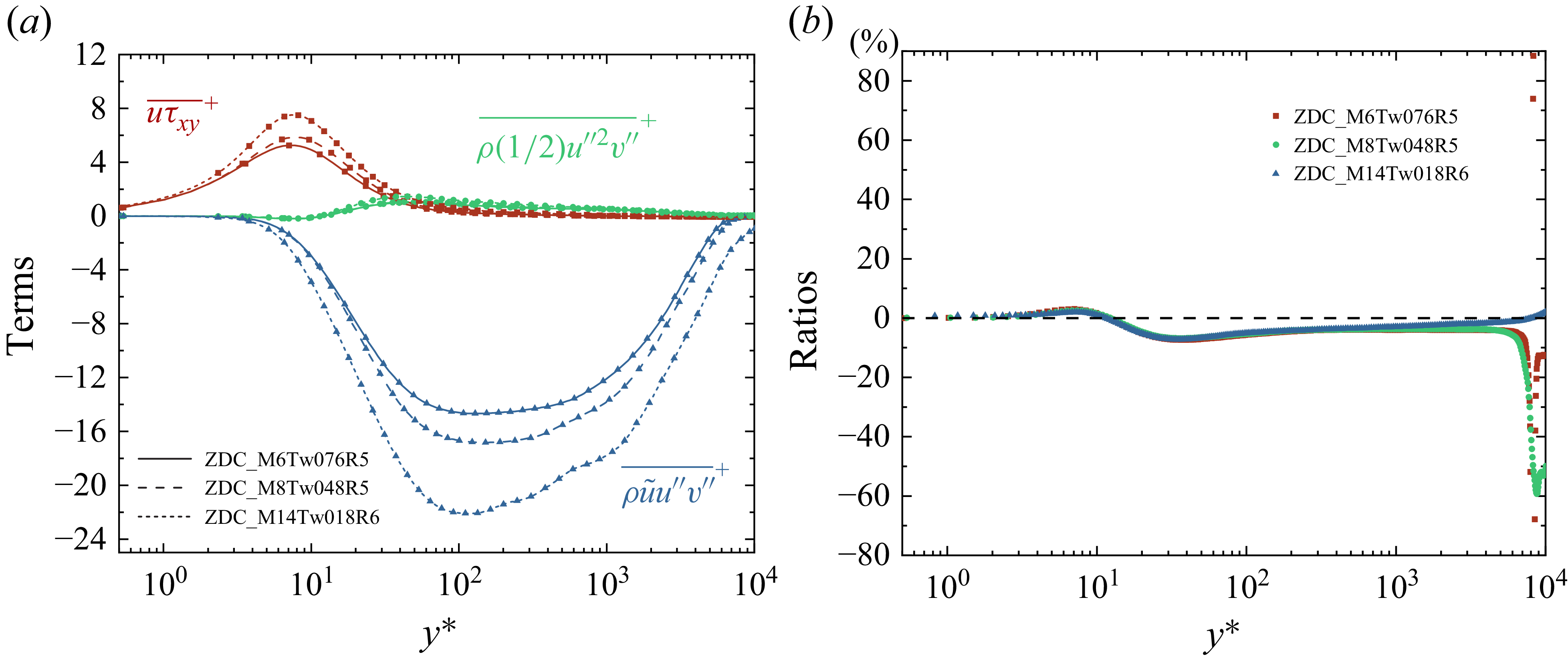


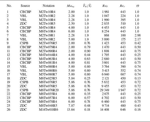


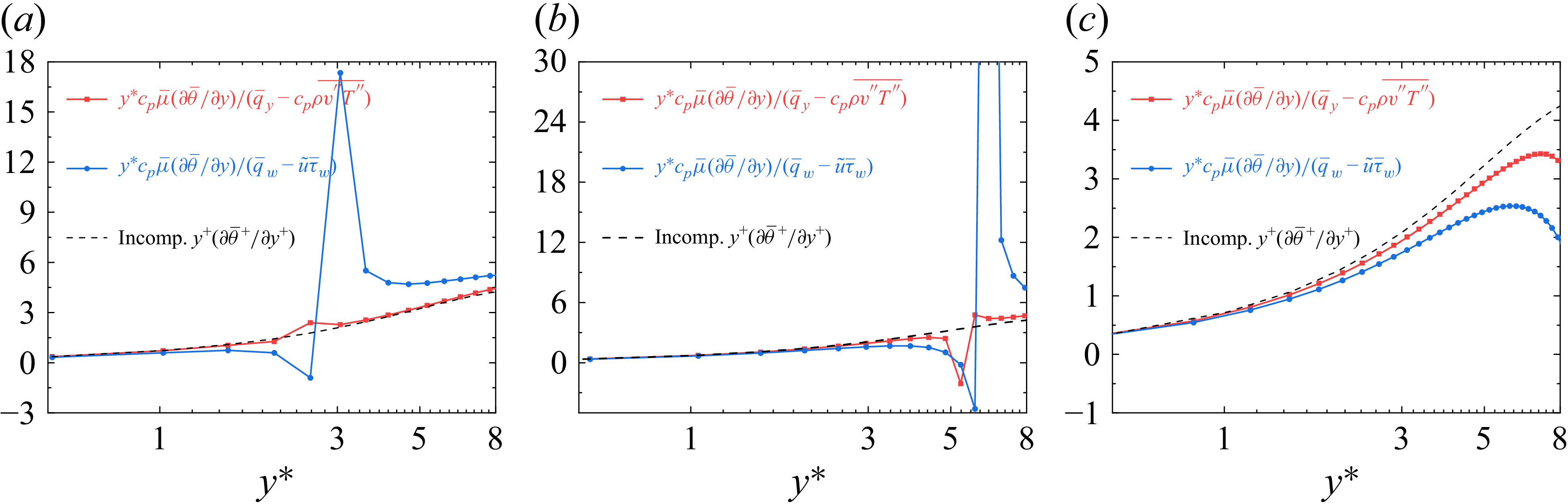


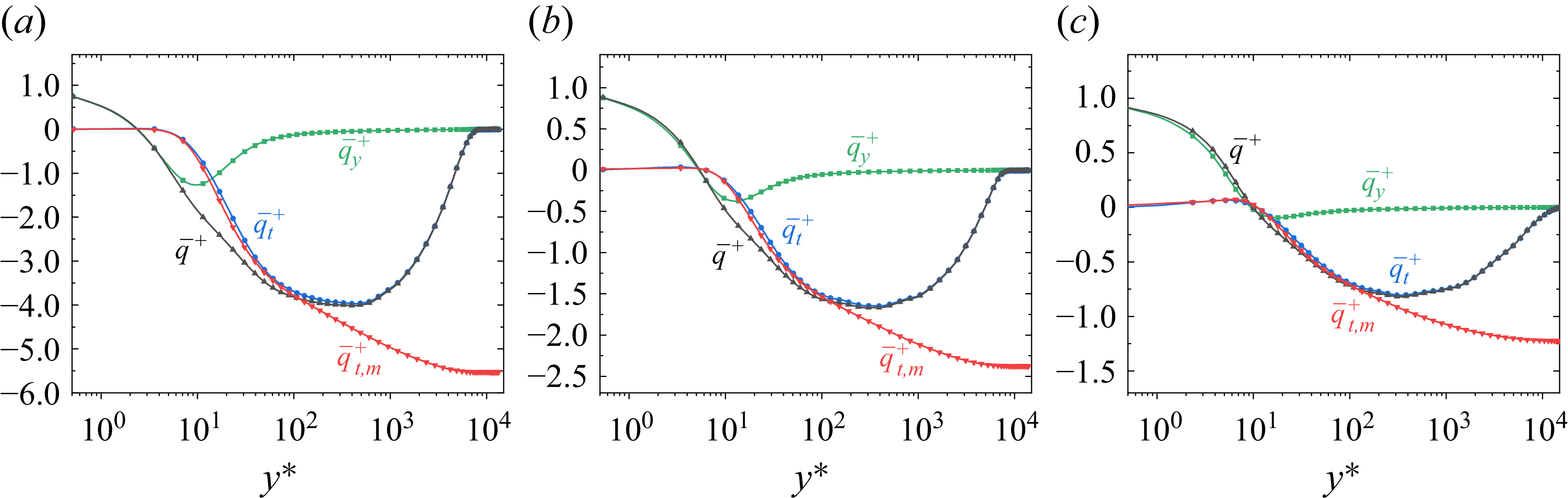


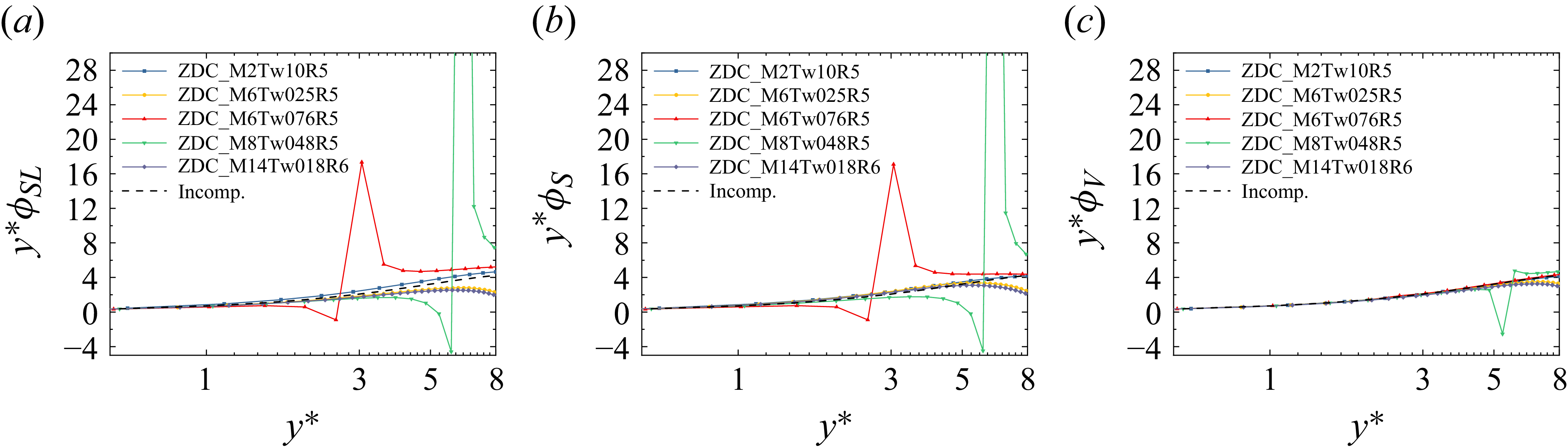


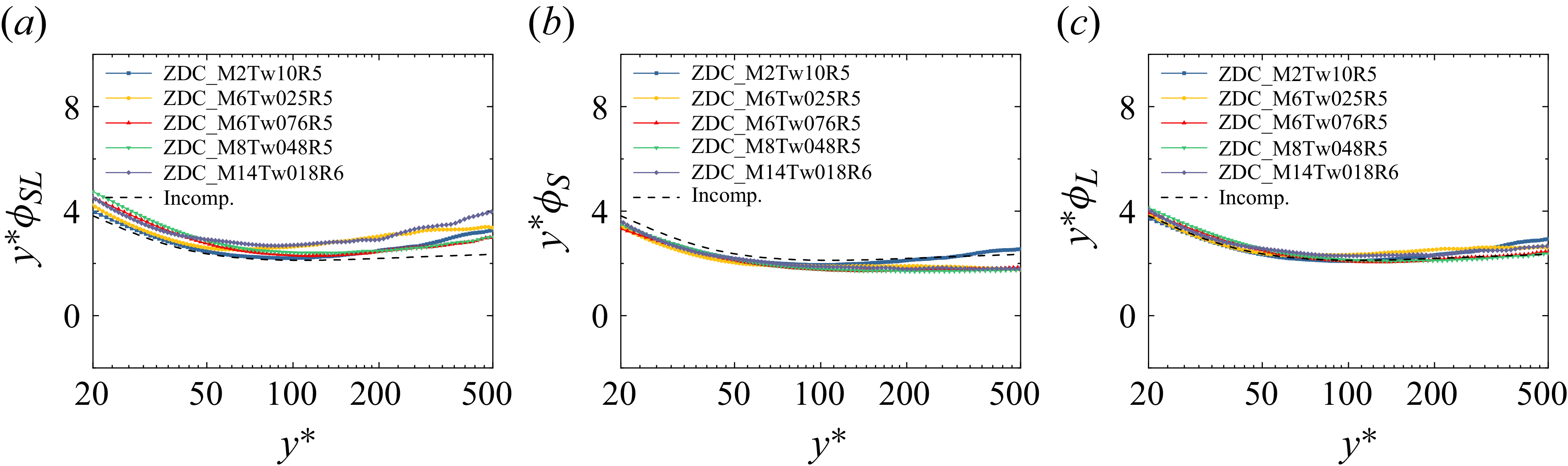


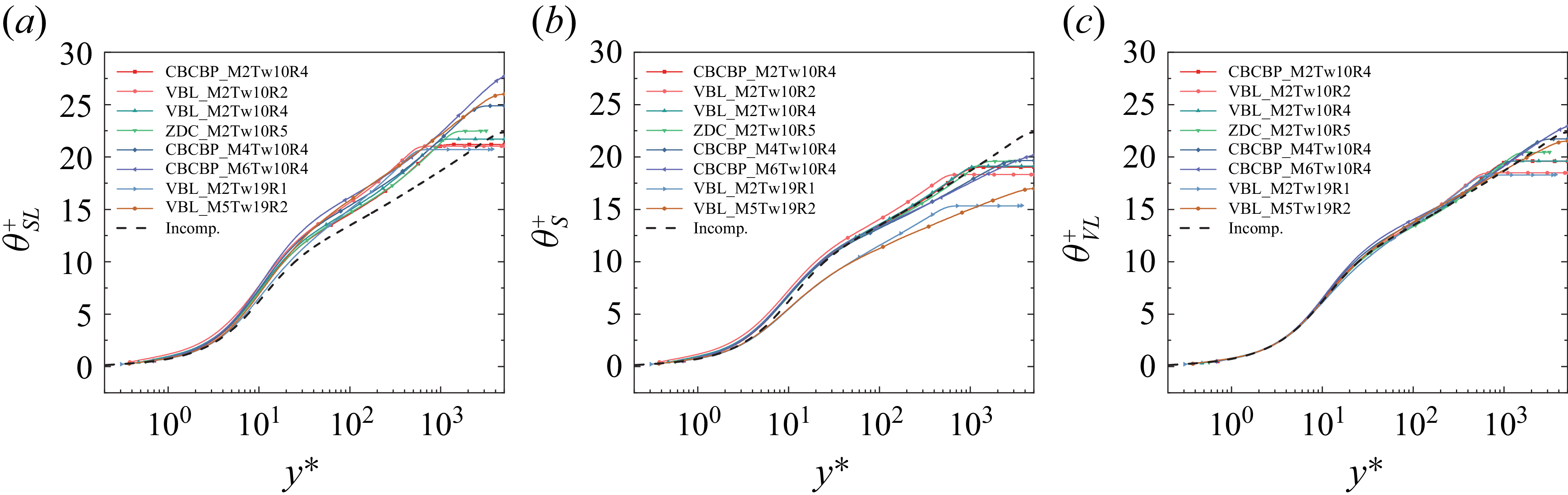
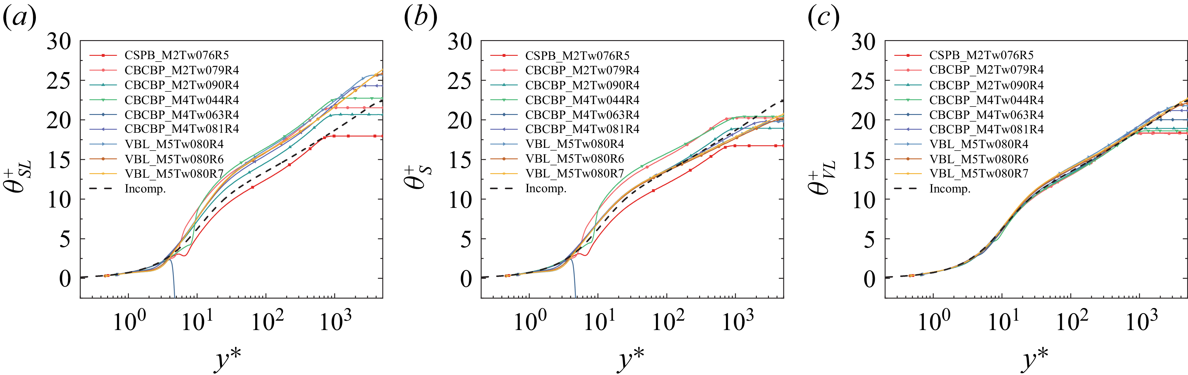
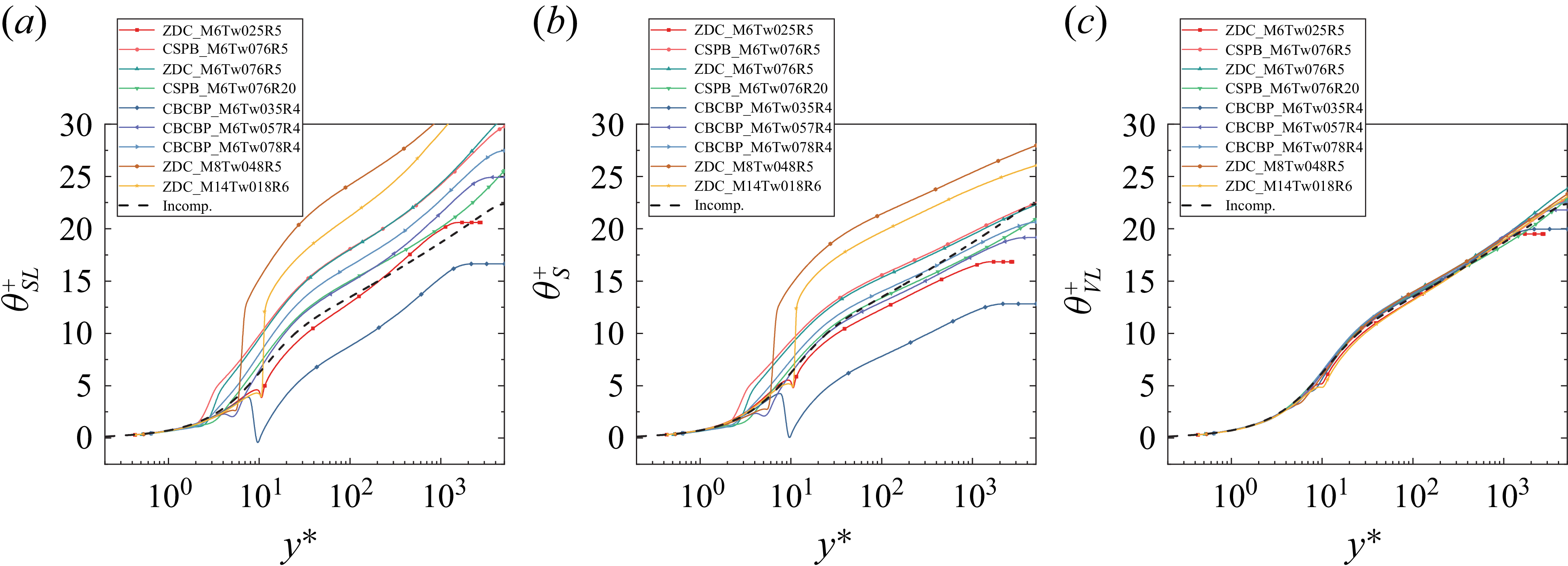
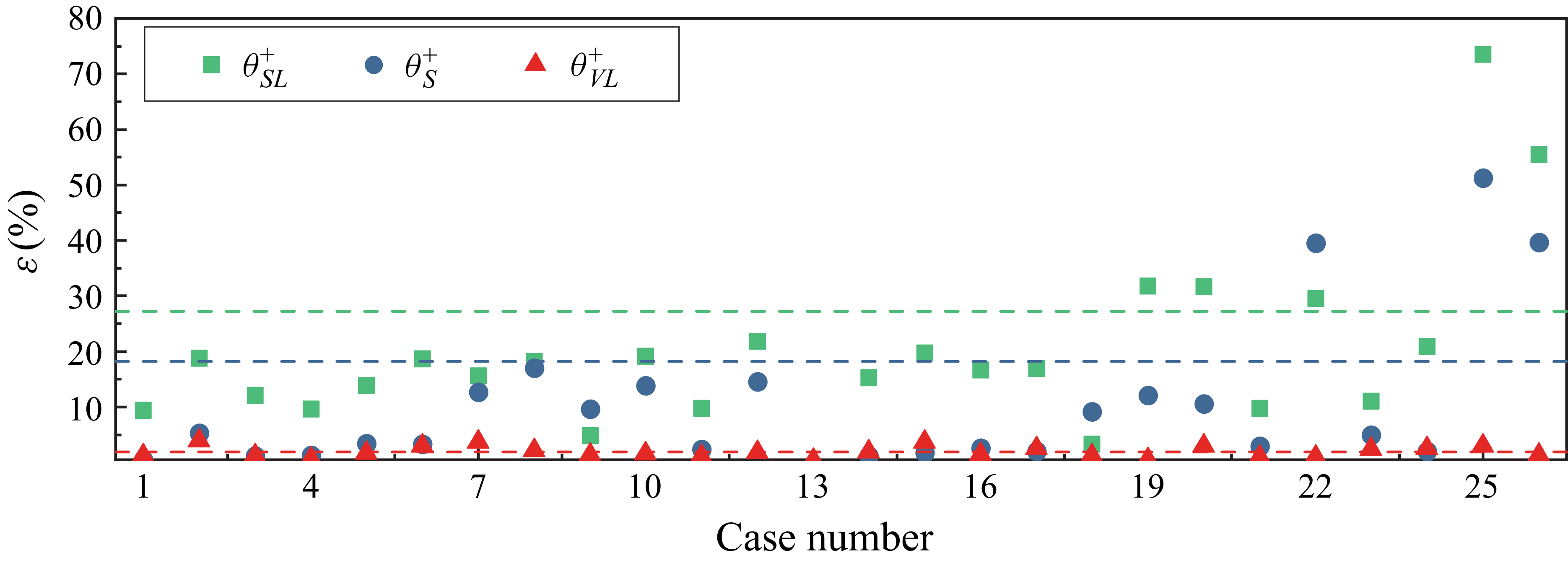


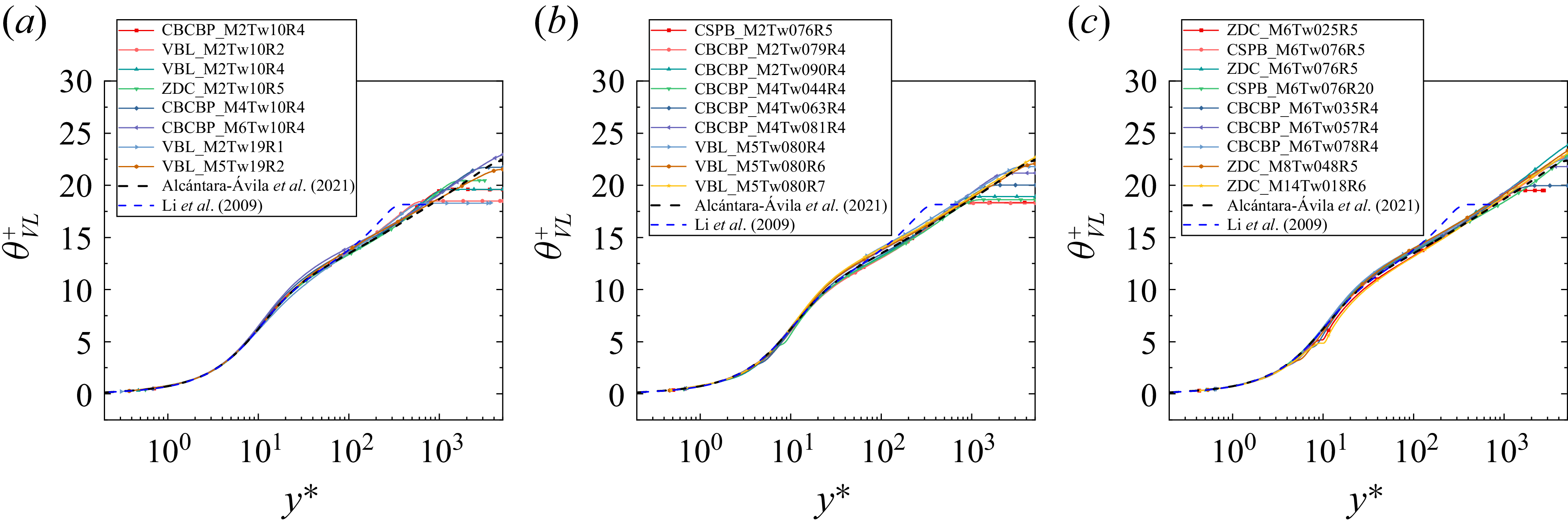

 Open access