2.1. The inverse Navier–Stokes problem

An $n$-dimensional velocimetry experiment usually provides noisy flow velocity images on a domain $I \subset \mathbb {R}^n$, depicting the measured flow velocity $\boldsymbol {u}^\star$ inside an object $\varOmega \subset I$ with boundary $\partial \varOmega = \varGamma \cup \varGamma _i \cup \varGamma _o$ (figure 1). An appropriate model is the Navier–Stokes problem

(2.1) \begin{equation} \left. \begin{array}{cl@{}} \boldsymbol{u}\boldsymbol{\cdot}\boldsymbol{\nabla}\boldsymbol{u}-\nu{\Delta} \boldsymbol{u} + \boldsymbol{\nabla} p = \boldsymbol{0} & \text{in}\ \varOmega,\\ \boldsymbol{\nabla} \boldsymbol{\cdot} \boldsymbol{u} = 0 & \text{in}\ \varOmega,\\ \boldsymbol{u} = \boldsymbol{0} & \text{on}\ \varGamma, \\ \boldsymbol{u} = \boldsymbol{g}_i & \text{on}\ \varGamma_i,\\ -\nu\partial_{\boldsymbol{\nu}}\boldsymbol{u}+p\boldsymbol{\nu} = \boldsymbol{g}_o & \text{on } \varGamma_o \end{array} \right\} \end{equation}

where $\boldsymbol {u}$ is the velocity, $p \unicode{x27FB} p/\rho$ is the reduced pressure, $\rho$ is the density, $\nu$ is the kinematic viscosity, $\boldsymbol {g}_i$ is the Dirichlet boundary condition at the inlet $\varGamma _i$, $\boldsymbol {g}_o$ is the natural boundary condition at the outlet $\varGamma _o$, $\boldsymbol {\nu }$ is the unit normal vector on $\partial \varOmega$ and ${\partial _{\boldsymbol {\nu }}\equiv \boldsymbol {\nu }\boldsymbol {\cdot } \boldsymbol {\nabla }}$ is the normal derivative.

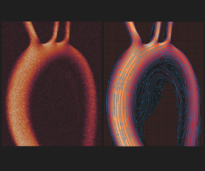
Figure 1. Given the images of a measured velocity field $\boldsymbol {u}^\star$, we solve an inverse Navier–Stokes problem to infer the boundary $\varGamma$ (or $\partial \varOmega$), the kinematic viscosity and the inlet velocity profile on $\varGamma _i$. The solution to this inverse problem is a reconstructed velocity field $\boldsymbol {u}^\circ$, from which the noise and the artefacts $(\boldsymbol {u}^\star -\mathcal {S}\boldsymbol {u}^\circ )$ have been filtered out.

We denote the data space by $\boldsymbol {D}$ and the model space by $\boldsymbol {M}$, and assume that both spaces are subspaces of $\boldsymbol {L}^2$. In the 2-D case, $\boldsymbol {u}^\star = (u^\star _x,u^\star _y)$ and we introduce the covariance operator

(2.2)\begin{equation} {{\mathcal{C}_{\boldsymbol{u}}} = \mathrm{diag}(\sigma^2_{u_x} \mathrm{I},\sigma^2_{u_y} \mathrm{I})}, \end{equation}

where $\sigma ^2_{u_x},\sigma ^2_{u_y}$ are the Gaussian noise variances of $u^\star _x,u^\star _y$, respectively, and $\mathrm {I}$ is the identity operator. The discrepancy between the measured velocity field ${\boldsymbol {u}^\star } \in \boldsymbol {D}$ and the modelled velocity field $\boldsymbol {u} \in \boldsymbol {M}$ is measured on the data space $\boldsymbol {D}$ using the reconstruction error functional

(2.3)\begin{equation} \mathscr{E}(\boldsymbol{u}) \equiv \tfrac{1}{2}\big\lVert \boldsymbol{u}^\star - \mathcal{S}\boldsymbol{u} \big\rVert^2_{\mathcal{C}_{\boldsymbol{u}}} := \tfrac{1}{2}\int_I (\boldsymbol{u}^\star - \mathcal{S}\boldsymbol{u})\mathcal{C}_{\boldsymbol{u}}^{ - 1}(\boldsymbol{u}^\star - \mathcal{S}\boldsymbol{u}), \end{equation}

where $\mathcal {S}: \boldsymbol {M}\to \boldsymbol {D}$ is the $L^2$-projection from the model space $\boldsymbol {M}$ to the data space $\boldsymbol {D}$. (Since the discretized space consists of bilinear quadrilateral finite elements (see § 2.7), this projection is a linear interpolation.)

Our goal is to infer the unknown parameters of the Navier–Stokes problem (2.1) such that the model velocity $\boldsymbol {u}$ approximates the noisy measured velocity $\boldsymbol {u}^\star$ in the covariance-weighted $L^2$-metric defined by $\mathscr {E}$. In the general case, the unknown model parameters of (2.1) are the shape of $\varOmega$, the kinematic viscosity $\nu$ and the boundary conditions $\boldsymbol {g}_i,\boldsymbol {g}_o$. This inverse Navier–Stokes problem leads to the nonlinearly constrained optimization problem

(2.4)\begin{equation} \text{find} \quad \boldsymbol{u}^\circ \equiv \underset{\varOmega,\boldsymbol{x}}{\mathrm{argmin}}~\mathscr{E}\left(\boldsymbol{u}(\varOmega;\boldsymbol{x})\right) \quad \text{such that }\boldsymbol{u}\text{ satisfies}\, (2.1),\end{equation}

where $\boldsymbol {u}^\circ$ is the reconstructed velocity field and $\boldsymbol {x}=(\boldsymbol {g}_i,\boldsymbol {g}_o,\nu )$. Like most inverse problems, (2.4) is ill-posed and hard to solve. To alleviate the ill-posedness of the problem, we need to restrict our search of the unknowns $(\varOmega,\boldsymbol {x})$ to function spaces of sufficient regularity.

2.2. Regularization

If $x(t) \in L^2(\mathbb {R})$ is an unknown parameter, one way to regularize the inverse problem (2.4) is to search for minimizers of the augmented functional $\mathscr {J} \equiv \mathscr {E} + \mathscr {R}$, where

(2.5)\begin{equation} \mathscr{R}(x) = \sum_{j=0}^k \int_{\mathbb{R}} \alpha_j \left|\partial_x^j(x-\bar{x})\right|^2 \end{equation}

is a regularization norm for a given (and fixed) prior assumption $\bar {x}(t) \in H^k(\mathbb {R})$, weights ${\alpha _j\in \mathbb {R}}$ and positive integer $k$. This simple idea can be quite effective because by minimizing $\mathscr {R}$, we force $x$ to lie in a subspace of $L^2$ having higher regularity, namely $H^k$, and as close to the prior value $\bar {x}$ as $\alpha _j$ allow. (The regularization term, given by (2.5), can be further extended to fractional Hilbert spaces by defining the norm $\big \lVert x \big \rVert _{H^s(\mathbb {R})} := \big \lVert (1+\lvert t \rvert ^s)\mathcal {F}x \big \rVert _{L^2(\mathbb {R})}$ for non-integer $s$, with $0< s<\infty$, and where $\mathcal {F}$ denotes the Fourier transform. Interestingly, under certain conditions, which are dictated by Sobolev's embedding theorem (Evans Reference Evans2010, Chapter 5), these Hilbert spaces can be embedded in the more familiar spaces of continuous functions.) However, as Stuart (Reference Stuart2010) points out, in this setting, the choice of $\alpha _j$, and even the form of $\mathscr {R}$, is arbitrary.

There is a more intuitive approach that recovers the form of the regularization norm $\mathscr {R}$ from a probabilistic viewpoint. In the setting of the Hilbert space $L^2$, the Gaussian measure $\gamma \sim \mathcal {N}(m,\mathcal {C})$ has the property that its finite-dimensional projections are multivariate Gaussian distributions, and it is uniquely defined by its mean $m \in L^2$, and its covariance operator $\mathcal {C}:L^2\to L^2$ (Appendix A). It can be shown that there is a natural Hilbert space $H_\gamma$ that corresponds to $\gamma$, and that (Bogachev Reference Bogachev1998; Hairer Reference Hairer2009)

(2.6)\begin{equation} H_\gamma = \sqrt{\mathcal{C}}(L^2). \end{equation}

In other words, if $x$ is a random function distributed according to $\gamma$, any realization of $x$ lies in $H_\gamma$, which is the image of $\sqrt {\mathcal {C}}$. Furthermore, the corresponding inner product

(2.7)\begin{equation} \big\langle x,x' \big\rangle_\mathcal{C} = \big\langle \mathcal{C}^{ - 1/2}x,\ \mathcal{C}^{ - 1/2}x' \big\rangle \end{equation}

is the covariance between $x$ and $x'$, and the norm $\big \lVert x \big \rVert ^2_\mathcal {C} = \big \langle x,x \big \rangle _\mathcal {C}$ is the variance of $x$. Therefore, if $x$ is an unknown parameter for which a priori statistical information is available, and if the Gaussian assumption can be justified, we can choose

(2.8)\begin{equation} \mathscr{R}(x) = \tfrac{1}{2}\big\lVert x-\bar{x} \big\rVert^2_\mathcal{C}. \end{equation}

In this way, $\mathscr {J}\equiv \mathscr {E}+\mathscr {R}$ increases as the variance of $x$ increases. Consequently, minimizing $\mathscr {J}$ penalizes improbable realizations.

As mentioned in § 2.1, the unknown model parameters of the Navier–Stokes problem (2.1) are the kinematic viscosity $\nu$, the boundary conditions $\boldsymbol {g}_i,\boldsymbol {g}_o$ and the shape of $\varOmega$. Since we consider the kinematic viscosity $\nu$ to be constant, the regularizing norm is simply

(2.9)\begin{equation} \frac{1}{2} \left|\nu - \bar{\nu}\right|^2_{\varSigma_\nu} = \frac{1}{2\sigma^2_{\nu}} \left|\nu - \bar{\nu}\right|^2_\mathbb{R}, \end{equation}

where $\bar {\nu }\in \mathbb {R}$ is a prior guess for $\nu$ and $\sigma ^2_{\nu }\in \mathbb {R}$ is the variance. For the Dirichlet boundary condition, $\boldsymbol {g}_i \in \boldsymbol {L}^2(\varGamma _i)$, we choose the exponential covariance function

(2.10)\begin{equation} C(x,x') = \frac{\sigma_{\boldsymbol{g}_i}^2}{2\ell} \exp\left(-\frac{\lvert x-x' \rvert}{\ell}\right) \end{equation}

with variance $\sigma _{\boldsymbol {g}_i}^2 \in \mathbb {R}$ and characteristic length $\ell \in \mathbb {R}$. For zero-Dirichlet (no-slip) or zero-Neumann boundary conditions on $\partial \varGamma _i$, (2.10) leads to the norm (Tarantola Reference Tarantola2005, Chapter 7.21)

(2.11)\begin{equation} \big\lVert \boldsymbol{g}_i \big\rVert_{\mathcal{C}_{\boldsymbol{g}_i}}^2 \simeq \frac{1}{\sigma_{\boldsymbol{g}_i}^2}\int_{\varGamma_i}\boldsymbol{g}^2_i + \ell^2 \left(\boldsymbol{\nabla}\boldsymbol{g}_i\right)^2 . \end{equation}

Using integration by parts, we find that the covariance operator is

(2.12)\begin{equation} \mathcal{C}_{\boldsymbol{g}_i} = \sigma_{\boldsymbol{g}_i}^2(\mathrm{I} - \ell^2\widetilde{\Delta})^{ - 1}, \end{equation}

where $\widetilde {\Delta }$ is the $L^2$-extension of the Laplacian $\Delta$ that incorporates the boundary condition $\boldsymbol {g}_i = \boldsymbol {0}$ on ${\partial \varGamma _i}$. For the natural boundary condition, $\boldsymbol {g}_o \in \boldsymbol {L}^2(\varGamma _o)$, we can use the same covariance operator, but equip $\widetilde {\Delta }$ with zero-Neumann boundary conditions, i.e. $\partial _{\boldsymbol {\nu }}\boldsymbol {g}_o = 0$ on $\partial \varGamma _o$. Lastly, for the shape of $\varOmega$, which we implicitly represent with a signed distance function ${\phi _{\pm }}$ (defined in § 2.4), we choose the norm

(2.13)\begin{equation} \frac{1}{2}\big\lVert \bar{\phi}_\pm - {\phi_{{\pm}}} \big\rVert^2_{\mathcal{C}_{\phi_{{\pm}}}}=\frac{1}{2\sigma^{2}_{\phi_{{\pm}}}}\big\lVert \bar{\phi}_\pm - {\phi_{{\pm}}} \big\rVert^2_{L^2(I)}, \end{equation}

where $\sigma _{\phi _{\pm }} \in \mathbb {R}$ and $\bar {\phi }_\pm \in L^2(I)$. Additional regularization for the boundary of $\varOmega$ (i.e. the zero level-set of ${\phi _{\pm }}$) is needed and it is described in § 2.4. Based on the above results, the regularization norm for the unknown model parameters is

(2.14)\begin{align} \mathscr{R}(\boldsymbol{x},{\phi_{{\pm}}}) &= \tfrac{1}{2}\left|\nu - \bar{\nu}\right|^2_{\varSigma_\nu} + \tfrac{1}{2}\big\lVert \boldsymbol{g}_i-\bar{\boldsymbol{g}}_i \big\rVert^2_{\mathcal{C}_{\boldsymbol{g}_i}} \nonumber\\ &\quad +\,\tfrac{1}{2}\big\lVert \boldsymbol{g}_o-\bar{\boldsymbol{g}}_o \big\rVert^2_{\mathcal{C}_{\boldsymbol{g}_o}}+\tfrac{1}{2}\big\lVert \bar{\phi}_\pm - {\phi_{{\pm}}} \big\rVert^2_{\mathcal{C}_{\phi_{{\pm}}}} . \end{align}

2.3. Euler–Lagrange equations for the inverse Navier–Stokes problem

Testing the Navier–Stokes problem (2.1) with functions ${(\boldsymbol {v},q) \in \boldsymbol {H}^1(\varOmega ) \times L^2(\varOmega )}$ and after integrating by parts, we obtain the weak form

(2.15)$$\begin{gather} \mathscr{M}(\varOmega)(\boldsymbol{u},p,\boldsymbol{v},q;\boldsymbol{x}) \equiv\int_\varOmega\left(\boldsymbol{v}\boldsymbol{\cdot}\left( \boldsymbol{u}\boldsymbol{\cdot}\boldsymbol{\nabla}\boldsymbol{u}\right) + \nu\boldsymbol{\nabla}\boldsymbol{v}\boldsymbol{:}\boldsymbol{\nabla} \boldsymbol{u} - (\boldsymbol{\nabla}\boldsymbol{\cdot}\boldsymbol{v}) p - q(\boldsymbol{\nabla}\boldsymbol{\cdot} \boldsymbol{u})\right) +\int_{\varGamma_o}\boldsymbol{v}\boldsymbol{\cdot}\boldsymbol{g}_o \nonumber\\ +\int_{\varGamma\cup\varGamma_i} \boldsymbol{v}\boldsymbol{\cdot}(-\nu\partial_{\boldsymbol{\nu}}\boldsymbol{u}+p\boldsymbol{\nu}) + \mathscr{N}_{\varGamma_i}(\boldsymbol{v},q,\boldsymbol{u};\boldsymbol{g}_i)+\mathscr{N}_{\varGamma}(\boldsymbol{v},q,\boldsymbol{u};\boldsymbol{0})={0}, \end{gather}$$

where $\mathscr {N}$ is the Nitsche (Reference Nitsche1971) penalty term

(2.16)\begin{equation} \mathscr{N}_{T}(\boldsymbol{v},q,\boldsymbol{u};\boldsymbol{z}) \equiv \int_{T} (-\nu\partial_{\boldsymbol{\nu}}\boldsymbol{v}+q\boldsymbol{\nu}+ \eta\boldsymbol{v})\boldsymbol{\cdot}(\boldsymbol{u}-\boldsymbol{z}), \end{equation}

which weakly imposes the Dirichlet boundary condition $\boldsymbol {z} \in \boldsymbol {L}^2(T)$ on a boundary $T$, given a penalization constant $\eta$. (The penalization $\eta$ is a numerical parameter with no physical significance (see § 2.7).) We define the augmented reconstruction error functional

(2.17)\begin{equation} \mathscr{J}(\varOmega)(\boldsymbol{u},p,\boldsymbol{v},q;\boldsymbol{x}) \equiv \mathscr{E}(\boldsymbol{u})+ \mathscr{R}(\boldsymbol{x},{\phi_{{\pm}}}) + \mathscr{M}(\varOmega)(\boldsymbol{u},p,\boldsymbol{v},q;\boldsymbol{x}), \end{equation}

which contains the regularization terms $\mathscr {R}$ and the model constraint $\mathscr {M}$, such that $\boldsymbol {u}$ weakly satisfies (2.1). To reconstruct the measured velocity field $\boldsymbol {u}^\star$ and find the unknowns $(\varOmega,\boldsymbol {x})$, we minimize $\mathscr {J}$ by solving its associated Euler–Lagrange system.

2.3.1. Adjoint Navier–Stokes problem

To derive the Euler–Lagrange equations for $\mathscr {J}$, we first define

(2.18)\begin{equation} \boldsymbol{\mathcal{U}}' = \left\{\boldsymbol{u}' \in \boldsymbol{H}^1(\varOmega): \boldsymbol{u}'\big\vert_{\varGamma\cup\varGamma_i} \equiv \boldsymbol{0} \right\} \end{equation}

to be the space of admissible velocity perturbations $\boldsymbol {u}'$ and $\mathcal {P}'\subset L^2(\varOmega )$ to be the space of admissible pressure perturbations $p'$, such that $(-\partial _{\boldsymbol {\nu }}\boldsymbol {u}'+p'\boldsymbol {\nu })\vert _{\varGamma _o}\equiv \boldsymbol {0}$. We start with

(2.19)\begin{align} \delta_{\boldsymbol{u}}\mathscr{E}\equiv\frac{{\rm d}}{{\rm d}\tau}\mathscr{E}(\boldsymbol{u}+\tau\boldsymbol{u}')\Big\vert_{\tau=0}&=\int_\varOmega -{\mathcal{C}^{ - 1}_{\boldsymbol{u}}}\left(\boldsymbol{u}^\star - \mathcal{S}\boldsymbol{u}\right)\boldsymbol{\cdot}\mathcal{S}\boldsymbol{u}'\nonumber\\ &= \int_\varOmega -\mathcal{S}^{\dagger}{\mathcal{C}^{ - 1}_{\boldsymbol{u}}}\left(\boldsymbol{u}^\star - \mathcal{S}\boldsymbol{u}\right)\boldsymbol{\cdot}\boldsymbol{u}'\equiv{\left\langle{D_{\boldsymbol{u}}\mathscr{E},\boldsymbol{u}'}\right\langle}_\varOmega . \end{align}

Adding together the first variations of $\mathscr {M}$ with respect to $(\boldsymbol {u},p)$,

(2.20a,b)\begin{align} \delta_{\boldsymbol{u}}\mathscr{M}\equiv\frac{{\rm d}}{{\rm d}\tau}\mathscr{M}({\cdot})(\boldsymbol{u}+\tau\boldsymbol{u}',\dots)\Big\vert_{\tau=0} , \quad \delta_{{p}}\mathscr{M}\equiv\frac{{\rm d}}{{\rm d}\tau}\mathscr{M}({\cdot})(\dots,p+\tau p',\dots)\Big\vert_{\tau=0}, \end{align}

and after integrating by parts, we find

(2.21)\begin{align} \delta_{\boldsymbol{u}}\mathscr{M}+\delta_{p}\mathscr{M}&=\int_\varOmega \left(-\boldsymbol{u}\boldsymbol{\cdot}\left(\boldsymbol{\nabla}\boldsymbol{v} + (\boldsymbol{\nabla}\boldsymbol{v})^{\dagger}\right) -\nu\Delta \boldsymbol{v} + \boldsymbol{\nabla} q \right)\boldsymbol{\cdot}\boldsymbol{u}' + \int_\varOmega (\boldsymbol{\nabla}\boldsymbol{\cdot}\boldsymbol{v})p' \nonumber\\ &\quad +\int_{\partial\varOmega} \left({(\boldsymbol{u}\boldsymbol{\cdot}\boldsymbol{\nu})\boldsymbol{v}}+{(\boldsymbol{u}\boldsymbol{\cdot}\boldsymbol{v})\boldsymbol{\nu}}+\nu\partial_{\boldsymbol{\nu}}\boldsymbol{v}-q\boldsymbol{\nu}\right)\boldsymbol{\cdot} \boldsymbol{u}' \nonumber\\ &\quad +\int_{\varGamma\cup\varGamma_i} \boldsymbol{v}\boldsymbol{\cdot}(-\nu\partial_{\boldsymbol{\nu}}\boldsymbol{u}'+p'\boldsymbol{\nu})+ \mathscr{N}_{\varGamma_i\cup\varGamma}(\boldsymbol{v},q,\boldsymbol{u}';\boldsymbol{0}) . \end{align}

Since $\mathscr {R}$ does not depend on $(\boldsymbol {u},p)$, we can use (2.19) and (2.21) to assemble the optimality conditions of $\mathscr {J}$ for $(\boldsymbol {u},p)$

(2.22)\begin{equation} {\left\langle{D_{\boldsymbol{u}}\mathscr{J},\boldsymbol{u}'}\right\rangle}_\varOmega = {0} ,\quad {\left\langle{D_{{p}}\mathscr{J},{p}'}\right\rangle}_\varOmega = 0. \end{equation}

For (2.22) to hold true for all perturbations ${(\boldsymbol {u}',p')\in \boldsymbol {\mathcal {U}}' \times \mathcal {P}'}$, we deduce that $(\boldsymbol {v},q)$ must satisfy the following adjoint Navier–Stokes problem

(2.23)\begin{equation} \left. \begin{array}{cl@{}} - \boldsymbol{u}\boldsymbol{\cdot}\left(\boldsymbol{\nabla}\boldsymbol{v} + (\boldsymbol{\nabla}\boldsymbol{v})^{\dagger}\right) -\nu\Delta \boldsymbol{v} + \boldsymbol{\nabla} q = - D_{\boldsymbol{u}}\mathscr{E} & \text{in}\ \varOmega,\\ \boldsymbol{\nabla} \boldsymbol{\cdot} \boldsymbol{v} = 0 & \text{in}\ \varOmega,\\ \boldsymbol{v} = \boldsymbol{0} & \text{on}\ \varGamma\cup\varGamma_i,\\ {(\boldsymbol{u}\boldsymbol{\cdot}\boldsymbol{\nu})\boldsymbol{v}}+{(\boldsymbol{u}\boldsymbol{\cdot}\boldsymbol{v})\boldsymbol{\nu}}+\nu\partial_{\boldsymbol{\nu}}\boldsymbol{v}-q\boldsymbol{\nu} = \boldsymbol{0} & \text{on}\ \varGamma_o. \end{array} \right\} \end{equation}

In this context, $\boldsymbol {v}$ is the adjoint velocity and $q$ is the adjoint pressure, which both vanish when $\boldsymbol {u}^\star \equiv \mathcal {S}\boldsymbol {u}$. Note also that we choose boundary conditions for the adjoint problem (2.23) that make the boundary terms of (2.21) vanish and that these boundary conditions are subject to the choice of $\boldsymbol {\mathcal {U}}'$, which, in turn, depends on the boundary conditions of the (primal) Navier–Stokes problem.

2.3.2. Shape derivatives for the Navier–Stokes problem

To find the shape derivative of an integral defined in $\varOmega$, when the boundary $\partial \varOmega$ deforms with speed $\mathscr {V}$, we use Reynold's transport theorem. For the bulk integral of $f:\varOmega \to \mathbb {R}$, we find

(2.24)\begin{equation} \frac{{\rm d}}{{\rm d}\tau}\left(\int_{\varOmega(\tau)} f\right)\bigg\vert_{\tau=0} = \int_\varOmega f' + \int_{\partial\varOmega}f~(\mathscr{V}\boldsymbol{\cdot}\boldsymbol{\nu}), \end{equation}

while for the boundary integral of $f$, we find (Walker Reference Walker2015, Chapter 5.6)

(2.25)\begin{equation} \frac{{\rm d}}{{\rm d}\tau}\left(\int_{\partial\varOmega(\tau)} f\right)\bigg\vert_{\tau=0} = \int_{\partial\varOmega} f' + (\partial_{\boldsymbol{\nu}}+\kappa)f (\mathscr{V}\boldsymbol{\cdot}\boldsymbol{\nu}), \end{equation}

where $f'$ is the shape derivative of $f$ (due to $\mathscr {V}$), $\kappa$ is the summed curvature of $\partial \varOmega$ and $\mathscr {V} \equiv \zeta \boldsymbol {\nu }$, with $\zeta \in L^2(\partial \varOmega )$, is the Hadamard parametrization of the speed field. Any boundary that is a subset of $\partial I$, i.e. the edge of the image $I$, is non-deforming and therefore the second term of the above integrals vanishes. The only boundary that deforms is $\varGamma \subset \partial \varOmega$. For brevity, let $\delta _\mathscr {V} I$ denote the shape perturbation of an integral $I$. Using (2.24) on $\mathscr {E}$, we compute

(2.26)\begin{equation} \delta_\mathscr{V}\mathscr{E} = {\left\langle{D_{\boldsymbol{u}}\mathscr{E},\boldsymbol{u}'}\right\rangle}_\varOmega, \end{equation}

where $D_{\boldsymbol {u}}\mathscr {E}$ is given by (2.19). Using (2.24) and (2.25) on $\mathscr {M}$, we obtain the shape derivatives problem for $(\boldsymbol {u}',p')$

(2.27)\begin{equation} \left. \begin{array}{cl@{}} \boldsymbol{u}'\boldsymbol{\cdot}\boldsymbol{\nabla}\boldsymbol{u}+\boldsymbol{u}\boldsymbol{\cdot}\boldsymbol{\nabla}\boldsymbol{u}'-\nu{\Delta} \boldsymbol{u}' + \boldsymbol{\nabla} p' = \boldsymbol{0} & \text{in}\ \varOmega,\\ \boldsymbol{\nabla} \boldsymbol{\cdot} \boldsymbol{u}' = 0 & \text{in}\ \varOmega,\\ \boldsymbol{u}' = - \partial_{\boldsymbol{\nu}}\boldsymbol{u}(\mathscr{V}\boldsymbol{\cdot}\boldsymbol{\nu}) & \text{on}\ \varGamma,\\ \boldsymbol{u}' = \boldsymbol{0} & \text{on}\ \varGamma_i, \\ -\nu\partial_{\boldsymbol{\nu}}\boldsymbol{u}'+p'\boldsymbol{\nu} = \boldsymbol{0} & \text{on}\ \varGamma_o, \end{array} \right\} \end{equation}

which can be used directly to compute the velocity and pressure perturbations for a given speed field $\mathscr {V}$. We observe that $(\boldsymbol {u}',p')\equiv \boldsymbol {0}$ when $\zeta \equiv \mathscr {V}\boldsymbol {\cdot } \boldsymbol {\nu }\equiv {0}$. Testing the shape derivatives problem (2.27) with $(\boldsymbol {v},q)$, and adding the appropriate Nitsche terms for the weakly enforced Dirichlet boundary conditions, we obtain

(2.28)$$\begin{align} \delta_\mathscr{V}\mathscr{M} &=\int_\varOmega\left(\boldsymbol{v}\boldsymbol{\cdot}\left( \boldsymbol{u}'\boldsymbol{\cdot}\boldsymbol{\nabla}\boldsymbol{u}+\boldsymbol{u}\boldsymbol{\cdot}\boldsymbol{\nabla}\boldsymbol{u}'\right) + \nu\boldsymbol{\nabla}\boldsymbol{v}\boldsymbol{:}\boldsymbol{\nabla} \boldsymbol{u}' - (\boldsymbol{\nabla}\boldsymbol{\cdot}\boldsymbol{v}) p' - q(\boldsymbol{\nabla}\boldsymbol{\cdot} \boldsymbol{u}')\right) \nonumber\\ &\quad +\int_{\varGamma\cup\varGamma_i} \boldsymbol{v}\boldsymbol{\cdot}(-\nu\partial_{\boldsymbol{\nu}}\boldsymbol{u}'+p'\boldsymbol{\nu}) + \mathscr{N}_{\varGamma_i}(\boldsymbol{v},q,\boldsymbol{u}';\boldsymbol{0})+\mathscr{N}_{\varGamma}(\boldsymbol{v},q,\boldsymbol{u}';-\zeta\partial_{\boldsymbol{\nu}}\boldsymbol{u})={0}. \end{align}$$

If we define $I_i$ to be the first four integrals in (2.21), integrating (2.28) by parts yields

(2.29)\begin{equation} \delta_\mathscr{V}\mathscr{M}= \sum_{i=1}^4 I_i + \mathscr{N}_{\varGamma_i}(\boldsymbol{v},q,\boldsymbol{u}';\boldsymbol{0})+\mathscr{N}_{\varGamma}(\boldsymbol{v},q,\boldsymbol{u}';-\zeta\partial_{\boldsymbol{\nu}}\boldsymbol{u})={0}, \end{equation}

and, due to the adjoint problem (2.23), we find

(2.30)\begin{equation} \delta_\mathscr{V}\mathscr{M}= - \delta_\mathscr{V}\mathscr{E} + \int_\varGamma \left(-\nu\partial_{\boldsymbol{\nu}}\boldsymbol{v}+q\boldsymbol{\nu}\right) \boldsymbol{\cdot}\zeta\partial_{\boldsymbol{\nu}}\boldsymbol{u}={0}, \end{equation}

since $\boldsymbol {u}'\vert _{\varGamma _i} \equiv \boldsymbol {0}$ and $\boldsymbol {u}\vert _{\varGamma } \equiv \boldsymbol {0}$. Therefore, the shape perturbation of $\mathscr {J}$ is

(2.31)\begin{equation} \delta_\mathscr{V} \mathscr{J} \equiv {\left\langle{D_{\mathscr{V}}\mathscr{J},\mathscr{V}\boldsymbol{\cdot}\boldsymbol{\nu}}\right\rangle}_\varGamma \equiv {\left\langle{D_{\zeta}\mathscr{J},\zeta}\right\rangle}_\varGamma = \delta_\mathscr{V} \mathscr{E} + \delta_\mathscr{V} \mathscr{M} + \delta_\mathscr{V} \mathscr{R} = 0, \end{equation}

which, due to (2.30) and $\delta _\mathscr {V} \mathscr {R} \equiv 0$, takes the form

(2.32)\begin{equation} {\left\langle{D_{\zeta}\mathscr{J},\zeta}\right\rangle}_\varGamma = {\left\langle{\partial_{\boldsymbol{\nu}}\boldsymbol{u}\boldsymbol{\cdot}\left(-\nu\partial_{\boldsymbol{\nu}}\boldsymbol{v}+q\boldsymbol{\nu}\right),\zeta}\right\rangle}_\varGamma , \end{equation}

where $D_{\zeta }\mathscr {J}$ is the shape gradient. Note that the shape gradient depends on the normal gradient of the (primal) velocity field and the pseudotraction, $(-\nu \boldsymbol {\nabla }\boldsymbol {v} + q\mathrm {I})\boldsymbol {\cdot } \boldsymbol {\nu }$, that the adjoint flow exerts on $\varGamma$.

2.3.3. Generalized gradients for the unknown model parameters ${x}$

The unknown model parameters $\boldsymbol {x}$ have an explicit effect on $\mathscr {M}$ and $\mathscr {R}$, and can therefore be obtained by taking their first variations. For the Dirichlet-type boundary condition at the inlet, we find

(2.33)\begin{align} {\left\langle{D_{\boldsymbol{g}_i}\mathscr{J},\boldsymbol{g}_i'}\right\rangle}_{\varGamma_i} &= {\left\langle{\nu\partial_{\boldsymbol{\nu}}\boldsymbol{v}-q\boldsymbol{\nu}- \eta\boldsymbol{v} + {\mathcal{C}^{ - 1}_{\boldsymbol{g}_i}}\left(\boldsymbol{g}_i-{\bar{\boldsymbol{g}}_i} \right),\boldsymbol{g}_i'}\right\rangle}_{\varGamma_i} \nonumber\\ &={\left\langle{{\mathcal{C}_{\boldsymbol{g}_i}}\left(\nu \partial_{\boldsymbol{\nu}}\boldsymbol{v}-q\boldsymbol{\nu}- \eta\boldsymbol{v}\right) + \boldsymbol{g}_i-\bar{\boldsymbol{g}}_i, \boldsymbol{g}_i'}\right\rangle}_{{\mathcal{C}_{\boldsymbol{g}_i}}}={\left\langle{\hat{D}_{\boldsymbol{g}_i}\mathscr{J},~\boldsymbol{g}_i'}\right\rangle}_{{\mathcal{C}_{\boldsymbol{g}_i}}}, \end{align}

where $-\hat {D}_{\boldsymbol {g}_i}\mathscr {J}$ is the steepest descent direction that corresponds to the covariance-weighted norm. For the natural boundary condition at the outlet, we find

(2.34)\begin{align} {\left\langle{D_{\boldsymbol{g}_o}\mathscr{J},\boldsymbol{g}_o'}\right\rangle}_{\varGamma_o} &= {\left\langle{\boldsymbol{v} + {\mathcal{C}^{ - 1}_{\boldsymbol{g}_o}}\left(\boldsymbol{g}_o-\bar{\boldsymbol{g}}_o\right),\boldsymbol{g}_o'}\right\rangle}_{\varGamma_o} \nonumber\\ &={\left\langle{{\mathcal{C}_{\boldsymbol{g}_o}}\boldsymbol{v} + \boldsymbol{g}_o-\bar{\boldsymbol{g}}_o,\boldsymbol{g}_o'}\right\rangle}_{{\mathcal{C}_{\boldsymbol{g}_o}}} = {\left\langle{\hat{D}_{\boldsymbol{g}_o}\mathscr{J}, \boldsymbol{g}_o'}\right\rangle}_{{\mathcal{C}_{\boldsymbol{g}_o}}}. \end{align}

Lastly, since the kinematic viscosity is considered to be constant within $\varOmega$, its generalized gradient is

(2.35)\begin{align} {\left\langle{D_{\nu}\mathscr{J}, \nu'}\right\rangle}_\mathbb{R} &= {\left\langle{\int_\varOmega \boldsymbol{\nabla}\boldsymbol{v}\boldsymbol{:}\boldsymbol{\nabla}\boldsymbol{u} + {\varSigma^{ - 1}_{\nu}} \left(\nu-\bar{\nu}\right), \nu'}\right\rangle}_\mathbb{R} \nonumber\\ & = {\left\langle{{\varSigma_{\nu}} \int_\varOmega \boldsymbol{\nabla}\boldsymbol{v}\boldsymbol{:}\boldsymbol{\nabla}\boldsymbol{u} + \nu-\bar{\nu}, \nu'}\right\rangle}_{{\varSigma_{\nu}}} = {\left\langle{\hat{D}_{\nu}\mathscr{J}, \nu'}\right\rangle}_{\varSigma_{\nu}} . \end{align}

For a given step size $\mathbb {R} \ni \tau > 0$, the steepest descent directions (2.33)–(2.35) can be used either to update an unknown parameter $x$ through

(2.36)\begin{equation} x_{k+1} = x_k + \tau s_k, \end{equation}

with $s_k = -\hat {D}_{x}\mathscr {J}$, or to reconstruct an approximation $\tilde {H}$ of the inverse Hessian matrix, in the context of a quasi-Newton method, and thereby to compute $s_k = -\tilde {H}\hat {D}_{x}\mathscr {J}$. We adopt the latter approach, which is discussed in § 2.5.

2.4. Geometric flow

To deform the boundary $\partial \varOmega$ using the simple update formula (2.36), we need a parametric surface representation. Here we choose to implicitly represent $\partial \varOmega$ using signed distance functions ${\phi _{\pm }}$. The object $\varOmega$ and its boundary $\partial \varOmega$ are then identified with a particular function ${\phi _{\pm }}$ such that

(2.37a,b)\begin{equation} \varOmega =\left\{x \in \varOmega:\ {\phi_{{\pm}}}(x) < 0 \right\},\quad \partial\varOmega = \left\{x \in \varOmega:\ {\phi_{{\pm}}}(x) = 0 \right\}. \end{equation}

2.4.1. Implicit representation of $\varOmega$ using signed distance functions

A signed distance function ${\phi _{\pm }}$ for $\varOmega$ can be obtained by solving the Eikonal equation

(2.38)\begin{equation} \lvert \boldsymbol{\nabla} {\phi_{{\pm}}}(x) \rvert = 1 \quad \text{subject to}\ {\phi_{{\pm}}}\big\vert_{\partial\varOmega} = 0 \quad x \in I. \end{equation}

One way to solve this problem is with level-set methods (Osher & Sethian Reference Osher and Sethian1988; Sethian Reference Sethian1996; Burger Reference Burger2001, Reference Burger2003; Burger & Osher Reference Burger and Osher2005; Yu, Juniper & Magri Reference Yu, Juniper and Magri2019). There is, however, a different approach, which relies on the heat equation (Varadhan Reference Varadhan1967b,Reference Varadhana; Crane, Weischedel & Wardetzky Reference Crane, Weischedel and Wardetzky2017). The main result that we draw from Varadhan (Reference Varadhan1967b), to justify the use of the heat equation for the approximation of ${\phi _{\pm }}$, states that

(2.39)\begin{equation} {d}(x,\partial\varOmega) = \lim_{\tau_1 \to 0} \left(-\frac{\sqrt{\tau_1}}{2}\log u(x,\tau_1) \right) ,\quad x \in I, \end{equation}

where ${d}(x,\partial \varOmega )$ is the Euclidean distance between any point $x \in I$ and $\partial \varOmega$, and $u$ is the solution of heat propagation away from $\partial \varOmega$

(2.40)\begin{equation} \left. \begin{array}{cl@{}} \left(I-\tau_1\Delta\right) u = 0 & \text{in}\ I, \\ u = 1 & \text{on}\ \partial \varOmega. \end{array} \right\} \end{equation}

Crane et al. (Reference Crane, Weischedel and Wardetzky2017) used the above result to implement a smoothed distance function computation method which they called the ‘heat method’. Here, we slightly adapt this method to compute signed distance functions ${\phi _{\pm }}$ in truncated domains (figure 2b). To compute ${\phi _{\pm }}$, we therefore solve (2.40) for $\tau _1 \ll 1$ and then obtain ${\phi _{\pm }}$ by solving

(2.41)\begin{equation} \left. \begin{array}{cl@{}} \boldsymbol{\nabla}\boldsymbol{\cdot}\boldsymbol{\nabla} {\phi_{{\pm}}} = \boldsymbol{\nabla} \boldsymbol{\cdot} X & \text{in}\ I,\\ \partial_{\boldsymbol{\nu}} {\phi_{{\pm}}} = X \boldsymbol{\cdot} \boldsymbol{\nu} & \text{on}\ \partial I,\\ {\phi_{{\pm}}} = 0 & \text{on}\ \partial \varOmega, \end{array} \right\} \quad X = - \text{sgn}(\psi) \dfrac{\boldsymbol{\nabla} u}{\lvert \boldsymbol{\nabla} u \rvert}, \end{equation}

with $X$ being the normalized heat flux and $\psi$ being a signed function such that $\psi (x)$ is negative for points $x$ in $\varOmega$ and positive for points $x$ outside ${\varOmega }$. This intermediate step (the solution of two Poisson problems (2.40)–(2.41) instead of one) is taken to ensure that $\lvert \boldsymbol {\nabla }{\phi _{\pm }} \rvert = 1$.

Figure 2. Geometric flow of $\partial \varOmega$ (figure 2a) relies on the computation of its signed distance field ${\phi _{\pm }}$ (figure 2b) and its normal vector extension ${\mathring {\boldsymbol {\nu }}}$ (figure 2c). The shape gradient $\zeta$ (figure 2d), which is initially defined on $\partial \varOmega$, is extended to the whole image $I$ (${\mathring {\zeta }}$ in figure 2e, f). Shape regularization is achieved by increasing the diffusion coefficient $\epsilon _{\zeta }$ to mitigate small-scale perturbations when assimilating noisy velocity fields $\boldsymbol {u}^\star$. Figure 2( f) shows results at a lower value of $\mbox {Re}_{\zeta }$ than figure 2(e). (a) Shape of $\partial \varOmega$. (b) Level-sets of ${\phi _{\pm }}$. (c) Magnitude of ${\phi _{\pm }}$ and ${\mathring {\boldsymbol {\nu }}}$. (d) Shape gradient $\zeta$ on $\partial \varOmega$. (e) ${\mathring {\zeta }}$ in $I$ ($\mbox {Re}_{\zeta }=1$). ( f) ${\mathring {\zeta }}$ in $I$ ($\mbox {Re}_{\zeta }=0.01$).

2.4.2. Propagating the boundary of $\varOmega$

To deform the boundary $\partial \varOmega$, we transport ${\phi _{\pm }}$ under the speed field ${\mathscr {V} \equiv \zeta \boldsymbol {\nu }}$. The convection-diffusion problem for ${\phi _{\pm }}(x,t)$ reads

(2.42)\begin{equation} \left. \begin{array}{cl@{}} \partial_t{\phi_{{\pm}}} + {\mathring{\mathscr{V}}}\boldsymbol{\cdot}\boldsymbol{\nabla}{\phi_{{\pm}}} -\epsilon_{\phi_{{\pm}}}\Delta{\phi_{{\pm}}} = 0 & \text{in}\ I\times (0,\tau],\\ {\phi_{{\pm}}} = {{\phi_{{\pm}}}}_0 \quad & \text{in}\ I\times \{t=0\}, \end{array} \right\} \quad \epsilon_{\phi_{{\pm}}} = \frac{\lvert \mathscr{V} \rvert_\infty \iota}{\textit{Re}_{\phi_{{\pm}}}}, \end{equation}

where ${{\phi _{\pm }}}_0$ denotes the signed distance function of the current domain $\varOmega$, $\epsilon _{\phi _{\pm }}$ is the diffusion coefficient, $\iota$ is a length scale, $\mbox {Re}_{\phi _{\pm }}$ is a Reynolds number and ${{\mathring {\mathscr {V}}}:I \to \mathbb {R}\times \mathbb {R}}$ is an extension of $\mathscr {V}: \partial \varOmega \to \mathbb {R}\times \mathbb {R}$. If we solve (2.42) for ${\phi _{\pm }}(x,\tau )$, we obtain the implicit representation of the perturbed domain $\varOmega _\tau$ at time $t=\tau$ (the step size), but to do so, we first need to extend $\mathscr {V}$ to the whole space of the image $I$.

To extend $\mathscr {V}$ to $I$, we extend the normal vector $\boldsymbol {\nu }$ and the scalar function $\zeta$, which are both initially defined on $\partial \varOmega$. The normal vector extension (figure 2c) is easily obtained by

(2.43)\begin{equation} {\mathring{\boldsymbol{\nu}}}(x) = \frac{\boldsymbol{\nabla} {\phi_{{\pm}}}}{\lvert \boldsymbol{\nabla}{\phi_{{\pm}}} \rvert} = \boldsymbol{\nabla} {\phi_{{\pm}}} ,\quad x \in I, \end{equation}

since $\lvert \boldsymbol {\nabla }{\phi _{\pm }} \rvert = 1$, and an outward-facing extension is given by

(2.44)\begin{equation} {\mathring{\boldsymbol{\nu}}}_o = \text{sgn}({\phi_{{\pm}}}){\mathring{\boldsymbol{\nu}}}. \end{equation}

We then use the extended normal vector ${\mathring {\boldsymbol {\nu }}}_o$ to extend $\zeta \in L^2(\partial \varOmega )$ to ${\mathring {\zeta }} \in L^2(I)$, using the convection-diffusion problem

(2.45)\begin{equation} \left. \begin{array}{cl@{}} \partial_t {\mathring{\zeta}} + {{\mathring{\boldsymbol{\nu}}}_o}\boldsymbol{\cdot}\boldsymbol{\nabla}{\mathring{\zeta}} - \epsilon_{\zeta} \Delta {\mathring{\zeta}} = 0 & \text{in}\ I\times (0,\tau_{\zeta}],\\ {\mathring{\zeta}} = \zeta & \text{on}\ \partial \varOmega\times (0,\tau_{\zeta}], \\ {\mathring{\zeta}} \equiv 0 & \text{in}\ I\times\{t=0\}, \end{array} \right\} \quad \epsilon_{\zeta} = \dfrac{\lvert {\mathring{\boldsymbol{\nu}}}_o \rvert_\infty \iota}{\textit{Re}_{\zeta}}. \end{equation}

In other words, we convect $\zeta$ along the predefined ${\mathring {\boldsymbol {\nu }}}_o$-streamlines and add isotropic diffusion for regularization (figure 2e, f). The choice of $\epsilon _{\phi _{\pm }}$ in (2.42) and $\epsilon _{\zeta }$ in (2.45) has been made for the shape regularization to depend only on the length scale $\iota$ and the Reynolds numbers $\mbox {Re}_{\phi _{\pm }},\mbox {Re}_{\zeta }$. More precisely, the shape regularization depends only on $\mbox {Re}_{\phi _{\pm }}$ and $\mbox {Re}_{\zeta }$ because we fix the length scale $\iota$ to equal the smallest possible length scale of the modelled flow, which is the numerical grid spacing $h$ for a uniform Cartesian grid. For illustration, if we consider $\zeta$ to be the concentration of a dye on $\partial \varOmega$ (figure 2d), using a simplified scaling argument similar to the growth of a boundary layer on a flat plate, we observe that the diffusing dye at distance $d$ from $\partial \varOmega$ will extend over a width $\delta$ such that

(2.46)\begin{equation} \delta \sim \sqrt{\frac{\epsilon_{\zeta} d}{\lvert {\mathring{\boldsymbol{\nu}}}_o \rvert_\infty}}=\sqrt{\frac{\iota d}{\textit{Re}_{\zeta}}}\quad \text{or}\quad \frac{\delta}{\iota} \sim \sqrt{\frac{\alpha}{\textit{Re}_{\zeta}}} \quad \text{when}\ d = \alpha \iota. \end{equation}

The above scaling approximation describes the dissipation rate of small-scale features such as roughness away from $\partial \varOmega$. This is therefore how $\mbox {Re}_{\phi _{\pm }}$ and $\mbox {Re}_{\zeta }$ control the regularity of the boundary $\partial \varOmega _\tau$ at time $t = \tau$, which is given by (2.42). We take $\tau _{\zeta }$ to be large enough to find a steady-state for (2.45). We recast the linear initial value problems (2.42) and (2.45) into their corresponding boundary value problems using backward-Euler temporal discretization because the time-dependent solution does not interest us here.

The extended shape gradient (2.32), after taking into account the regularizing term for ${\phi _{\pm }}$, is therefore given by

(2.47) \begin{align}{\left\langle{D_{\mathring{\zeta}}\mathscr{J}, {\mathring{\zeta}}'}\right\rangle}_I &={\left\langle{{\mathring{\zeta}} + \mathcal{C}^{ -1}_{\phi_{{\pm}}}\left(\bar{\phi}_\pm - {\phi_{{\pm}}}\right), {\mathring{\zeta}}'}\right\rangle}_I \nonumber\\ &={\left\langle{\mathcal{C}_{\phi_{{\pm}}}{\mathring{\zeta}} +\bar{\phi}_\pm - {\phi_{{\pm}}},{\mathring{\zeta}}'}\right\rangle}_{\mathcal{C}_{\phi_{{\pm}}}} ={\left\langle{\hat{D}_{\mathring{\zeta}}\mathscr{J},{\mathring{\zeta}}'}\right\rangle}_{\mathcal{C}_{\phi_{{\pm}}}},\end{align}

where ${\mathring {\zeta }}$ is the extension of the shape gradient $\zeta (x) = \partial _{\boldsymbol {\nu }}\boldsymbol {u}\boldsymbol {\cdot } (-\nu \partial _{\boldsymbol {\nu }}\boldsymbol {v}+q\boldsymbol {\nu })$, for $x$ on $\varGamma$.

2.5. Segregated approach for the Euler–Lagrange system

The inverse Navier–Stokes problem for the reconstruction and the segmentation of noisy velocity images $\boldsymbol {u}^\star$ can be written as the saddle point problem (Benzi, Golubt & Liesen Reference Benzi, Golubt and Liesen2005)

(2.48)\begin{equation} \text{find} \quad \boldsymbol{u}^\circ\equiv \mathrm{arg}\ \underset{\varOmega,\boldsymbol{x}}{\mathrm{min}}\, \underset{\boldsymbol{v},q}{\mathrm{max}}~\mathscr{J}(\varOmega)(\boldsymbol{u},p,\boldsymbol{v},q;\boldsymbol{x}), \end{equation}

where $\mathscr {J}$ is given by (2.17). The above optimization problem leads to an Euler–Lagrange system whose optimality conditions were formulated in § 2.3. We briefly describe our segregated approach to solve this Euler–Lagrange system in algorithm 1.

Algorithm 1: Reconstruction and segmentation of noisy flow velocity images.

To precondition the steepest descent directions (2.33)–(2.35) and (2.47), we reconstruct the approximated inverse Hessian $\tilde {H}$ of each unknown using the BFGS quasi-Newton method (Fletcher Reference Fletcher2000) with damping (Nocedal & Wright Reference Nocedal and Wright2006). Due to the large scale of the problem, it is only possible to work with the matrix-vector product representation of $\tilde {H}$. Consequently, the search directions are given by

(2.49) \begin{equation} \boldsymbol{s} = - \begin{pmatrix} \tilde{H}_{\mathring{\zeta}} & {\cdot} & {\cdot} & {\cdot} \\ {\cdot} & \tilde{H}_{\boldsymbol{g}_i} & {\cdot} & {\cdot} \\ {\cdot} & {\cdot} & \tilde{H}_{\boldsymbol{g}_o} & {\cdot} \\ {\cdot} & {\cdot} & {\cdot} & \tilde{H}_\nu \end{pmatrix} \begin{pmatrix} \hat{D}_{\mathring{\zeta}} \mathscr{J}\\ \hat{D}_{\boldsymbol{g}_i}\mathscr{J}\\ \hat{D}_{\boldsymbol{g}_o}\mathscr{J}\\ \hat{D}_\nu\mathscr{J} \end{pmatrix}, \end{equation}

and the unknown variables $\boldsymbol {x}$ are updated according to (2.36). The signed distance function ${\phi _{\pm }}$ is perturbed according to (2.42), with ${\mathring {\mathscr {V}}} \equiv -(\tilde {H}_{\mathring{\zeta}}\hat {D}_{\mathring{\zeta}}\mathscr {J}){\mathring {\boldsymbol {\nu }}}$. We start every line search with a global step size $\tau = 1$ and halve the step size until ${\mathscr {J}(({\phi _{\pm }},\boldsymbol {x})_{k+1}) < \mathscr {J}(({\phi _{\pm }},\boldsymbol {x})_{k})}$. To update the flowfield $\boldsymbol {u}_k$ to $\boldsymbol {u}_{k+1}$, we solve the Oseen problem for the updated parameters $({\phi _{\pm }},\boldsymbol {x})_{k+1}$

(2.50)\begin{equation} \boldsymbol{u}_k\boldsymbol{\cdot}\boldsymbol{\nabla}\boldsymbol{u}_{k+1}-\nu{\Delta} \boldsymbol{u}_{k+1} + \boldsymbol{\nabla} p_{k+1} = \boldsymbol{0},\quad \boldsymbol{\nabla}\boldsymbol{\cdot}\boldsymbol{u}_{k+1} = 0, \end{equation}

with the boundary conditions given by (2.1). Algorithm 1 terminates if either the covariance-weighted norm for the perturbations of the model parameters is below the user-specified tolerance or the line search fails to reduce $\mathscr {J}$.

2.6. Uncertainty estimation

We now briefly describe how the reconstructed inverse Hessian $\tilde {H}$ can provide estimates for the uncertainties of the model parameters. To simplify the description, let $x$ denote an unknown parameter distributed according to $\mathcal {N}(x_k,\mathcal {C}_x)$. The linear approximation to the data $\boldsymbol {u}^\star$ is given by

(2.51a,b)\begin{equation} \boldsymbol{u}^\star= \mathcal{Z}x + \varepsilon,\quad \varepsilon \sim \mathcal{N}(0,{\mathcal{C}_{\boldsymbol{u}}}), \end{equation}

where $\boldsymbol {u} = \mathcal {Z}x$, where $\mathcal {Z}$ is the operator that encodes the linearized Navier–Stokes problem around the solution $\boldsymbol {u}_k$. To solve (2.48), we update $x$ as

(2.52) \begin{equation} x_{k+1} = x_k + \mathcal{C}\mathcal{Z}^{\dagger}{\mathcal{C}^{ - 1}_{\boldsymbol{u}}}(\boldsymbol{u}^\star - \mathcal{Z}x_k),\quad \text{with}\ \mathcal{C} = (\mathcal{Z}^{\dagger}{\mathcal{C}^{ - 1}_{\boldsymbol{u}}}\mathcal{Z}+\mathcal{C}^{ - 1}_x)^{ - 1}, \end{equation}

where $\mathcal {Z}^{\dagger}$ is the operator that encodes the adjoint Navier–Stokes problem and $\mathcal {C}$ is the posterior covariance operator. It can be shown that (Tarantola Reference Tarantola2005, Chapter 6.22.8)

(2.53) \begin{equation} \mathcal{C} = (\mathcal{Z}^{\dagger}{\mathcal{C}^{ - 1}_{\boldsymbol{u}}}\mathcal{Z}+\mathcal{C}^{ - 1}_x)^{ - 1} = (\mathcal{C}_x\mathcal{Z}^{\dagger}{\mathcal{C}^{ - 1}_{\boldsymbol{u}}}\mathcal{Z}+\mathrm{I})^{ - 1}\mathcal{C}_x \simeq \tilde{H}_x\mathcal{C}_x, \end{equation}

where $\tilde {H}_x$ is the reconstructed inverse Hessian for $x$. Note that $\tilde {H}$ by itself approximates $(\mathcal {C}_x\mathcal {Z}^{\dagger} {\mathcal {C}^{-1}_{\boldsymbol {u}}}\mathcal {Z}+\mathrm {I})^{-1}$ and not $\mathcal {C}$, because we use the steepest ascent directions $\hat {D}_{({\cdot })}\mathscr {J}$ (prior-preconditioned gradients), instead of the gradients ${D}_{({\cdot })}\mathscr {J}$, in the BFGS formula. Therefore, if $\tilde {\mathcal {C}}\equiv \tilde {H}_x\mathcal {C}_x$ is the approximated covariance matrix, then samples $x^s_{k+1}$ from the posterior distribution can be drawn using the Karhunen–Loève expansion

(2.54)\begin{equation} x^s_{k+1} = x_k + \sum_k \eta_k~\sqrt{\lambda_k}\varphi_k, \quad \text{with}\ \eta_k \sim \mathcal{N}(0,1), \end{equation}

where $(\lambda,\varphi )_k$ is the eigenvalue/eigenvector pair of $\tilde {\mathcal {C}}$. The variance of $x_{k+1}$ can then be directly computed from the samples.

2.7. Numerics

To solve the above boundary value problems numerically, we use an immersed boundary finite element method. In particular, we implement the fictitious domain cut-cell finite element method (FEM), which was introduced by Burman (Reference Burman2010) and Burman & Hansbo (Reference Burman and Hansbo2012) for the Poisson problem, and extended by Burman, and Massing et al. (Reference Massing, Larson, Logg and Rognes2014); Massing, Schott & Wall (Reference Massing, Schott and Wall2018) to the Stokes and the Oseen problems. We define $\mathcal {T}_h$ to be a tessellation of $I$ produced by square cells (pixels) $K \in \mathcal {T}_h$, having sides of length $h$. We also define the set of cut-cells $\mathcal {T}_h^\triangleright$ consisting of the cells that are cut by the boundary $\partial \varOmega$, and $\mathcal {T}_h^{{\Box }}$ the set of cells that are found inside $\varOmega$ and which remain intact (not cut) (see figure 1). We assume that the boundary $\partial \varOmega$ is well-resolved, i.e. $\ell _{\partial \varOmega }/h \gg 1$ where $\ell _{\partial \varOmega }$ is the smallest length scale of $\partial \varOmega$. For the detailed assumptions on $\partial \varOmega$, we cite Burman & Hansbo (Reference Burman and Hansbo2012). The discretized space is generated by assigning a bilinear quadrilateral finite element $\mathcal {Q}_1$ to every cell $K$. To compute the integrals, we use standard Gaussian quadrature for cells $K \in \mathcal {T}_h^{\Box}$, while for cut-cells $K \in \mathcal {T}_h^\triangleright$, where integration must be considered only for the intersection $K\cap \varOmega$, we use the approach of Mirtich (Reference Mirtich1996), which relies on the divergence theorem and simply replaces the integral over $K \cap \varOmega$ with an integral over $\partial (K\cap \varOmega )$. The boundary integral on $\partial (K\cap \varOmega )$ is then easily computed using one-dimensional Gaussian quadrature (Massing, Larson & Logg Reference Massing, Larson and Logg2013). Since we use an inf-sup unstable finite element pair ($\mathcal {Q}_1$–$\mathcal {Q}_1$) (Brenner & Scott Reference Brenner and Scott2008), we use a pressure-stabilizing Petrov–Galerkin formulation (Tezduyar Reference Tezduyar1991; Codina Reference Codina2002) and $\boldsymbol {\nabla }$-div stabilization for preconditioning (Benzi & Olshanskii Reference Benzi and Olshanskii2006; Heister & Rapin Reference Heister and Rapin2013). Typical values and formulae for numerical parameters, e.g. Nitsche's penalization $\eta$, are given by Massing et al. (Reference Massing, Larson, Logg and Rognes2014, Reference Massing, Schott and Wall2018). Here, we take $\eta = \gamma \nu /h$ (Massing et al. Reference Massing, Schott and Wall2018), with $\gamma = 100$. To solve the Navier–Stokes problem, we use fixed-point iteration (Oseen linearization) and at each iteration, we solve the coupled system using the Schur complement; with an iterative solver (LGMRES) for the outer loops and a direct sparse solver (UMFPACK) for the inner loops. The immersed FEM solver and all the necessary numerical operations of algorithm 1 are implemented in Python, using its standard libraries for scientific computing, namely SciPy (Virtanen et al. Reference Virtanen2020) and NumPy (Harris et al. Reference Harris2020). Computationally intensive functions are accelerated using Numba (Lam, Pitrou & Seibert Reference Lam, Pitrou and Seibert2015) and CuPy (Okuta et al. Reference Okuta, Unno, Nishino, Hido and Loomis2017).

3.1. Synthetic data for 2-D flow in a converging channel

We start by testing algorithm 1 on a flow through a symmetric converging channel having a taper ratio of $0.67$. To generate synthetic 2-D Navier–Stokes data, we solve the Navier–Stokes problem (2.1) for a parabolic inlet velocity profile ($\boldsymbol {g}_i$), zero-pseudotraction boundary conditions at the outlet ($\boldsymbol {g}_o \equiv \boldsymbol {0}$) and $\mbox {Re} \simeq 534$, to obtain the ground truth velocity $\boldsymbol {u}^\bullet$. We then generate the synthetic data $\boldsymbol {u}^\star$ by corrupting the components of $\boldsymbol {u}^\bullet$ with white Gaussian noise such that $\textrm {SNR}_x=\textrm {SNR}_y=3$. For this test case, we are only trying to infer $\varOmega$ and $\boldsymbol {g}_i$. Note that, in our method, the initial guess $x_0$ of an unknown $x$ equals the mean of its prior distribution $\bar {x}$, i.e. $x_0\equiv \bar {x}$. We start the algorithm using bad initial guesses (high uncertainty in priors) for both the unknown parameters (see table 1). The initial guess for $\varOmega$, labelled $\varOmega _0$, is a rectangular domain with height equal to $0.7D$, centred in the image domain. For ${\boldsymbol {g}_i}_0$, we take a parabolic velocity profile with a peak velocity of approximately $2U$ that fits the inlet of $\varOmega _0$. For comparison, $\boldsymbol {g}_i^\bullet$ has a peak velocity of $1.5U$, while it is also defined on a different domain, namely $\varOmega ^\bullet$.

Table 1. Input parameters for the inverse 2-D Navier–Stokes problem.

The algorithm manages to reconstruct and segment the noisy flow images in 39 iterations, with a total reconstruction error $\mathcal {E}^\bullet \simeq 1.44\,\%$. The results are presented in figures 3 and 4. We observe that the inverse Navier–Stokes problem performs very well in filtering the noise $(\boldsymbol {u}^\star -\mathcal {S}\boldsymbol {u}^\circ )$ (figure 3c, f), providing noiseless images for each component of the velocity (figure 3b,e). As we expect, the discrepancies ${\mathcal {C}^{-1}_{\boldsymbol {u}}}(\boldsymbol {u}^\star -\mathcal {S}\boldsymbol {u}^\circ )$ (figure 3c, f) consist mainly of Gaussian white noise, except at the corners of the outlet (figure 3f), where there is a weak correlation. For a more detailed presentation of the denoising effect, we plot slices of the reconstructed velocity (figure 4c) and the ground truth velocity (figure 4d). The reconstructed pressure $p^\circ$, which is consistent with the reconstructed velocity $\boldsymbol {u}^\circ$ to machine precision accuracy, is, in effect, indistinguishable from the ground truth $p^\bullet$ (figure 5).

Figure 3. Reconstruction (algorithm 1) of synthetic noisy velocity images depicting the flow (from left to right) in a converging channel. Figures 3(a,b) and 3(d,e) show the horizontal, $u_x$, and vertical, $u_y$, velocities and share the same colourmap (colourbar not shown). Figure 3(c, f) shows the discrepancy between the noisy velocity images and the reconstruction (colourbars apply only to figure 3c, f). (a) Synthetic image $u^\star _x$. (b) Our reconstruction $u_x^\circ$. (c) Discrepancy $\sigma _{u_x}^{-1}(u^\star _x - \mathcal {S}u_x^\circ )$. (d) Synthetic image $u^\star _y$. (e) Our reconstruction $u_y^\circ$. ( f) Discrepancy $\sigma _{u_y}^{-1}(u^\star _y - \mathcal {S}u_y^\circ )$.

Figure 4. Reconstruction (algorithm 1) of synthetic images depicting the flow (from left to right) in a converging channel. Figure 4(a) depicts the reconstructed boundary $\partial \varOmega ^\circ$ (cyan line), the $2\sigma$ confidence region computed from the approximated posterior covariance $\tilde {\mathcal {C}}_{\mathring{\zeta}} \equiv \tilde {H}_{\mathring{\zeta}} \mathcal {C}_{\phi _{\pm }}$ (blue region), the ground truth boundary $\partial \varOmega ^\bullet$ (yellow line) and the initial guess $\partial \varOmega _0$ (white line). Figure 4(b) shows the reconstruction error as a function of iteration number. Velocity slices are drawn for 10 equidistant cross-sections (labelled with the letters A to J) for both the reconstructed images (figure 4c) and the ground truth (figure 4d), coloured red for positive values and blue for negative. (a) Velocity magnitude $\lvert \boldsymbol {u}^\circ \rvert$ and shape $\partial \varOmega ^\circ$. (b) Reconstruction error history. (c) Noisy data (grey) and reconstruction. (d) Ground truth velocity distributions.

Figure 5. (a) Reconstructed and (b) ground truth reduced hydrodynamic pressure ($p$) for the flow (from left to right) in the converging channel in figure 4. (a) Our reconstruction $p^\circ$. (b) Ground truth $p^\bullet$.

Having obtained the reconstructed velocity $\boldsymbol {u}^\circ$, we can compute the wall shear rate $\gamma _w^\circ$ on the reconstructed boundary $\partial \varOmega ^\circ$, which we compare with the ground truth $\gamma _w^\bullet$ in figure 6. Using the upper ($\partial \varOmega ^\circ _+$) and lower ($\partial \varOmega ^\circ _-$) limits of the $2\sigma$ confidence region for $\partial \varOmega ^\circ$ (figure 4a), we estimate a confidence region for $\gamma _w^\circ$; although this has to be interpreted carefully. Note that, for example, $\partial \varOmega ^\circ _+$ and $\partial \varOmega ^\circ _-$ can be smoother than the mean $\partial \varOmega ^\circ$, and, therefore, $\partial \varOmega ^\circ$ may be found outside this confidence region. A better estimate of the confidence region could be obtained by sampling the posterior distribution of $\partial \varOmega ^\circ$ solving a Navier–Stokes problem for each sample $\partial \varOmega _k$ and finding the distribution of $\gamma ^\circ _w$. Since the latter approach would be computationally intensive, we only provide our estimate, which requires the solution of only two Navier–Stokes problems.

Figure 6. Wall shear rate $\gamma _w \equiv \boldsymbol {\tau }\boldsymbol {\cdot } \partial _{\boldsymbol {\nu }}\boldsymbol {u}$, where $\boldsymbol {\tau }$ is the unit tangent vector of $\partial \varOmega$, for the converging channel flow in figure 4. The wall shear stress is found by multiplying this by the viscosity. The reconstructed wall shear rate ($\gamma _w^\circ$) is calculated on $\partial \varOmega ^\circ$ and for $\boldsymbol {u}^\circ$, while the ground truth ($\gamma _w^\bullet$) is calculated on $\partial \varOmega ^\bullet$ and for $\boldsymbol {u}^\bullet$. The blue region is bounded by the two wall shear rate distributions for $\boldsymbol {u}^\circ$, calculated on the upper ($\partial \varOmega ^\circ _+$) and lower ($\partial \varOmega ^\circ _-$) limits of the $2\sigma$ confidence region of $\partial \varOmega ^\circ$. Note that the reconstructed solution can sometimes be found outside the blue region because the reconstructed shape $\partial \varOmega ^\circ$ may be less regular than $\partial \varOmega ^\circ _+$ or $\partial \varOmega ^\circ _-$. (a) Lower boundary. (b) Upper boundary.

3.2. Synthetic data for 2-D flow in a simulated abdominal aortic aneurysm

Next, we test algorithm 1 in a channel that resembles the cross-section of a small abdominal aortic aneurysm, with $D_{max}/D\simeq 1.5$, where $D_{max}$ is the maximum diameter at the midsection. We generate synthetic images for $\boldsymbol {u}^\star$ as in § 3.1, again for ${\textrm {SNR}_x=\textrm {SNR}_y=3}$, but now for $\mbox {Re} = 153$. The ground truth domain $\varOmega ^\bullet$ has horizontal symmetry but the inlet velocity profile deliberately breaks this symmetry. The inverse problem is the same as that in § 3.1 but with different input parameters (see table 2). The initial guess $\varOmega _0$ is a rectangular domain with height equal to $0.85D$, centred in the image domain. For ${\boldsymbol {g}_i}_0$, we take a skewed parabolic velocity profile with a peak velocity of approximately $2U$ that fits the inlet of $\varOmega _0$.

Table 2. Input parameters for the inverse 2-D Navier–Stokes problem.

The algorithm manages to reconstruct and segment the noisy flow images in 39 iterations, with total reconstruction error $\mathcal {E}^\bullet \simeq 2.87\,\%$. The results are presented in figures 7 and 8. We observe that the discrepancy (figure 7c, f) consists mainly of Gaussian white noise. Again, some correlations are visible in the discrepancy of the $y$-velocity component at the upper inlet corner and the upper boundary of the simulated abdominal aortic aneurysm. The latter correlations (figure 7f) can be explained by the associated uncertainty in the predicted shape $\partial \varOmega ^\circ$ (figure 8a), which is well estimated for the upper boundary but slightly underestimated for the upper inlet corner. It is interesting to note that the upward skewed velocity profile at the inlet creates a region of low velocity magnitude on the lower boundary. The velocity profiles in this region produce low wall shear stresses, as seen in figures 8(c,d), and 10(b). These conditions are particularly challenging when one tries to infer the true boundary $\partial \varOmega ^\bullet$ because the local SNR is low ($\textrm {SNR} \ll 1$), meaning that there is considerable information loss there. Despite the above difficulties, algorithm 1 manages to approximate the posterior distribution of $\partial \varOmega ^\circ$ well, and successfully predicts extra uncertainty in this region (figure 8a). Again, the reconstructed pressure $p^\circ$ is indistinguishable from the ground truth $p^\bullet$ (figure 9).

Figure 7. As for figure 3 but for the synthetic images depicting the flow (from left to right) in the simulated 2-D model of an abdominal aortic aneurysm. (a) Synthetic image $u^\star _x$. (b) Our reconstruction $u_x^\circ$. (c) Discrepancy $\sigma _{u_x}^{-1}(u^\star _x - \mathcal {S}u_x^\circ )$. (d) Synthetic image $u^\star _y$. (e) Our reconstruction $u_y^\circ$. ( f) Discrepancy $\sigma _{u_y}^{-1}(u^\star _y - \mathcal {S}u_y^\circ )$.

Figure 8. As for figure 4 but for the synthetic images depicting the flow (from left to right) in the simulated 2-D model of an abdominal aortic aneurysm. (a) Velocity magnitude $\lvert \boldsymbol {u}^\circ \rvert$ and shape $\partial \varOmega ^\circ$. (b) Reconstruction error history. (c) Noisy data (grey) and reconstruction. (d) Ground truth velocity distributions.

Figure 9. (a) Reconstructed and (b) ground truth reduced hydrodynamic pressure ($p$) for the flow (from left to right) in the simulated 2-D model of an abdominal aortic aneurysm in figure 8. (a) Our reconstruction $p^\circ$. (b) Ground truth $p^\bullet$.

Figure 10. As for figure 6 but for the synthetic images depicting the flow (from left to right) in the simulated 2-D model of an abdominal aortic aneurysm in figure 8. (a) Lower boundary. (b) Upper boundary.

Using the reconstructions $\boldsymbol {u}^\circ$ and $\partial \varOmega ^\circ$, we compute the wall shear rate and we compare it with the ground truth in figure 10(b). We observe that the reconstructed solution approximates the ground truth well, even for very low SNRs ($\textrm {SNR}=3$). Note that the waviness of the ground truth $\gamma _w^\bullet$ is due to the relatively poor resolution of the level set function that we intentionally used to implicitly define this domain.

3.3. Synthetic data for 2-D flow in a simulated aortic aneurysm

Next, we test algorithm 1 in a channel that resembles the cross-section of an aorta that has an aneurysm in its ascending part. This test case is designed to demonstrate that the algorithm is applicable to realistic geometries with multiple inlets/outlets and for abnormal flow conditions (e.g. separation and recirculation zones). We generate synthetic images for $\boldsymbol {u}^\star$ as in § 3.1, but for ${\textrm {SNR}_x=\textrm {SNR}_y=2.5}$ and for $\mbox {Re} = 500$. For increased Reynolds numbers ($\mbox {Re} = 1000, 1500$), we observed vortex shedding within the aneurysm and we could not find a steady flow solution to generate synthetic images of steady flow. The inverse problem is the same as that in § 3.1 but with different input parameters (see table 3). The initial guess for the boundary of $\varOmega _0$ (figure 11a) is generated by using the Chan–Vese segmentation method (Chan & Vese Reference Chan and Vese2001; Getreuer Reference Getreuer2012a; Van Der Walt et al. Reference Van Der Walt, Schönberger, Nunez-Iglesias, Boulogne, Warner, Yager, Gouillart and Yu2014) on the noisy mask of the ground truth domain $\varOmega ^\bullet$ (figure 11b). The prior standard deviation $\sigma _{\phi _{\pm }}$ corresponds to the length of approximately $7$ pixels of the noisy mask. The initial guess for the inlet velocity profile ${\boldsymbol {g}_i}_0$ is also shown in figure 11(a). Using the prior information of the boundary and the inlet velocity profile, algorithm 1 generates an initial guess for the Navier–Stokes velocity field (figure 12a,b) during its zeroth iteration.

Figure 11. Initial guesses (input for algorithm 1) for the geometry ($\partial \varOmega _0$) and the inlet velocity profile (${\boldsymbol {g}_i}_0$) versus their corresponding ground truth (figure 11a) for the flow in the simulated 2-D model of an aortic aneurysm. The initial guess $\partial \varOmega _0$ (figure 11a) is generated by segmenting the noisy mask (figure 11b) of the ground truth domain $\varOmega ^\bullet$. (a) Initial guesses (priors) for $\partial \varOmega$ and $\boldsymbol {g}_i$. (b) Noisy mask of $\varOmega ^\bullet$.

Figure 12. Zeroth iteration (N–S solution for the initial guesses in figure 11) velocity images (figure 12a,b), streamlines (figure 12c) and discrepancies with the data (figure 12d–f) for the flow in the simulated 2-D model of an aortic aneurysm. Streamlines are plotted on top of the velocity/discrepancy magnitude image and streamline thickness increases as the velocity magnitude increases. Figures 12(a–c) (colourbar not shown) and 12(d–f) (colourbar shown on the right) share the same colourmap. (a) $(u_x)_0$. (b) $(u_y)_0$. (c) $\boldsymbol {u}_0$. (d) $\sigma _{u_x}^{-1}(u^\star _x - \mathcal {S}(u_x)_0)$. (e) $\sigma _{u_y}^{-1}(u^\star _y - \mathcal {S}(u_y)_0)$. ( f) ${\mathcal {C}^{-1}_{\boldsymbol {u}}}(\boldsymbol {u}^\star -\mathcal {S}\boldsymbol {u}_0)$.

Table 3. Input parameters for the inverse 2-D Navier–Stokes problem.

The algorithm manages to reconstruct and segment the noisy flow images in 15 iterations, with a total reconstruction error $\mathcal {E}^\bullet \simeq 5.73\,\%$. The results are presented in figures 13 and 14. We observe that the discrepancy of the last iteration (figure 13c, f) consists mainly of Gaussian white noise. Some correlations are visible in the discrepancy of the $x$-velocity component near the stagnation points of the upper branches, but these correlations are explained by the extra uncertainty in the predicted shape $\partial \varOmega ^\circ$ (figure 14a). By comparing figures 13(c, f) with figure 12(d,e), we confirm that the algorithm has successfully assimilated the remaining information from the noisy velocity measurements. Figure 15 shows the pressure of the zeroth iteration (figure 15a), and the reconstructed pressure $p^\circ$ (figure 15b), which compares well to the ground truth pressure $p^\bullet$ (figure 15c).

Figure 13. Reconstruction (final iteration of algorithm 1) of synthetic noisy velocity images depicting the flow in the simulated 2-D model of an aortic aneurysm. Figures 13(a,b) and 13(d,e) show the horizontal, $u_x$, and vertical, $u_y$, velocities and share the same colourmap (colourbar not shown). Figure 13(c, f) shows the discrepancy between the noisy velocity images and the reconstruction (colourbars apply only to figure 13c, f). (a) Synthetic image $u^\star _x$. (b) Our reconstruction $u_x^\circ$. (c) Discrepancy $\sigma _{u_x}^{-1}(u^\star _x - \mathcal {S}u_x^\circ )$. (d) Synthetic image $u^\star _y$. (e) Our reconstruction $u_y^\circ$. ( f) Discrepancy $\sigma _{u_y}^{-1}(u^\star _y - \mathcal {S}u_y^\circ )$.

Figure 14. Reconstruction (final iteration of algorithm 1) of synthetic images depicting the flow in the simulated 2-D model of an aortic aneurysm. Figure 14(a) depicts the reconstructed boundary $\partial \varOmega ^\circ$ (cyan line), the $2\sigma$ confidence region computed from the approximated posterior covariance $\tilde {\mathcal {C}}_{\mathring{\zeta}} \equiv \tilde {H}_{\mathring{\zeta}} \mathcal {C}_{\phi _{\pm }}$ (blue region) and the ground truth boundary $\partial \varOmega ^\bullet$ (yellow line). Figure 14(b) shows the reconstruction error as a function of iteration number. (a) Velocity magnitude $\lvert \boldsymbol {u}^\circ \rvert$ and shape $\partial \varOmega ^\circ$. (b) Reconstruction error history.

Figure 15. (a) Zeroth iteration (N–S solution for the initial guesses in figure 11), (b) reconstructed (final iteration of algorithm 1) and (c) ground truth reduced hydrodynamic pressure for the simulated 2-D model of an aortic aneurysm in figure 14. All panels share the same colourmap (symmetric logarithmic scale) and the same colourbar. (a) Zeroth iteration $p_0$. (b) Our reconstruction $p^\circ$. (c) Ground truth $p^\bullet$.

We further compare the performance of algorithm 1 with a state-of-the-art image denoising algorithm, namely total variation denoising using Bregman iteration (TV-B) (Getreuer Reference Getreuer2012b; Van Der Walt et al. Reference Van Der Walt, Schönberger, Nunez-Iglesias, Boulogne, Warner, Yager, Gouillart and Yu2014) in figure 16. We first observe that algorithm 1 denoises the velocity field without losing contrast near the walls of the aorta and accurately identifies the low-speed vortical structure within the aneurysm, which is obscured by noise. We then test three different values of the TV-B parameter $\lambda /\lambda _0$, which controls the total variation regularization, and observe that even though TV-B manages to denoise the velocity field and reveal certain large scale vortices, there is considerable loss of contrast near the walls of the aorta and a systematic error (e.g. decreasing peak velocity) that increases as $\lambda$ decreases. (The parameter $\lambda _0=\lambda _0(\sigma )$, where $\sigma$ is the noise standard deviation in the image, is given by Getreuer (Reference Getreuer2012b) as an optimal value for $\lambda$.)

Figure 16. Streamlines for the flow in the simulated 2-D model of an aortic aneurysm (figures 13 and 14), and comparison with total variation denoising using Bregman iteration (TV-B) with different weights $\lambda$. Streamlines are plotted on top of the velocity magnitude image and streamline thickness increases as the velocity magnitude increases. (a) Synthetic data $\boldsymbol {u}^\star$. (b) Our reconstruction $\boldsymbol {u}^\circ$. (c) Ground truth $\boldsymbol {u}^\bullet$. (d) TV-B $\lambda /\lambda _0=0.1$. (e) TV-B $\lambda /\lambda _0=0.01$. ( f) TV-B $\lambda /\lambda _0=0.001$.

Using the reconstructions $\boldsymbol {u}^\circ$ and $\partial \varOmega ^\circ$, we compute the reconstructed wall shear rate ($\gamma _w^\circ$) and compare it with the ground truth ($\gamma _w^\bullet$) (figure 17). We observe that $\gamma _w^\circ$ approximates $\gamma _w^\bullet$ well and that discrepancies are well accounted for by the $\gamma _w^\circ \pm 2\sigma$-bounds.

Figure 17. Wall shear rate $\gamma _w \equiv \boldsymbol {\tau }\boldsymbol {\cdot } \partial _{\boldsymbol {\nu }}\boldsymbol {u}$, where $\boldsymbol {\tau }$ is the unit tangent vector of $\partial \varOmega$, for the flow in the simulated 2-D model of an aortic aneurysm in figure 14. The wall shear stress is found by multiplying this by the viscosity. The reconstructed wall shear rate ($\gamma _w^\circ$) is calculated on $\partial \varOmega ^\circ$ and for $\boldsymbol {u}^\circ$, while the ground truth ($\gamma _w^\bullet$) is calculated on $\partial \varOmega ^\bullet$ and for $\boldsymbol {u}^\bullet$. The $\pm 2\sigma$-bounds are calculated on the upper ($\partial \varOmega ^\circ _+$) and lower ($\partial \varOmega ^\circ _-$) limits of the confidence region of $\partial \varOmega ^\circ$. All panels share the same colourmap (symmetric logarithmic scale) and the same colourbar. (a) Zeroth iteration $(\gamma _w)_0$. (b) Our reconstruction $\gamma ^\circ _w$. (c) Ground truth $\gamma ^\bullet _w$. (d) Lower confidence bound $\gamma ^\circ _w-2\sigma$. (e) Upper confidence bound $\gamma ^\circ _w+2\sigma$.

3.4. Magnetic resonance velocimetry experiment

We measured the flow through a converging nozzle using magnetic resonance velocimetry (Fukushima Reference Fukushima1999; Mantle & Sederman Reference Mantle and Sederman2003; Elkins & Alley Reference Elkins and Alley2007). The nozzle converges from an inner diameter of 25 mm to an inner diameter of 13 mm, over a length of 40 mm (figure 18b). On either side of the converging section, the entrance-to-exit length equals 10 times the local diameter (figure 18b) to ensure the absence of entrance/exit effects. We acquired velocity images for a Reynolds number of 162 (defined at the nozzle outlet). We used a 40 wt% glycerol in water solution (Cheng Reference Cheng2008; Volk & Kähler Reference Volk and Kähler2018) as the working fluid to increase the viscosity and minimize the effect of thermal convection in the resulting velocity field due to the temperature difference between the magnet bore and the working fluid. The nozzle is made of polyoxymethylene to minimize magnetic susceptibility differences between the nozzle wall and the working fluid (Wapler et al. Reference Wapler, Leupold, Dragonu, von Elverfeld, Zaitsev and Wallrabe2014). Figure 18(a) depicts the schematic of the flow loop of the MRV experiment. To pump the water/glycerol solution, we used a Watson Marlow 505S peristaltic pump (Watson Marlow, Falmouth UK) with a 2 l dampening vessel at its outlet to dampen flow oscillations introduced by the peristaltic pump. To make the flow uniform, we installed porous polyethylene distributor plates (SPC technologies, Fakenham UK) at the entrance and the exit of the nozzle.

Figure 18. Schematic of the rig that we use to conduct the MRV experiment consisting of: (1) 20 l holding tank; (2) peristaltic pump; (3) 2 l vessel; (4) clamp valves; (5) porous polyethylene distributor; (6) radiofrequency probe; (7) converging nozzle; (8) $4.7$ T superconducting magnet; (9) volumetric cylinder for flow measurements. Figure 18(b) shows a sketch of the converging nozzle with the active area of the spectrometer shown by a red box. The pulse sequence that we use for 2-D velocity imaging is shown in figure 18(c). (a) Magnet and flow loop. (b) Converging nozzle. (c) Spin-echo pulse sequence with slice selective refocusing and flow encoding.

We acquired the velocity images on a Bruker Spectrospin DMX200 with a $4.7$ T superconducting magnet, which is equipped with a gradient set providing magnetic field gradients of a maximum strength of 13.1 G cm$^{-1}$ in three orthogonal directions, and a birdcage radiofrequency coil tuned to a ${}^{1}\mathrm {H}$ frequency of 199.7 MHz with a diameter and a length of 6.3 cm. To acquire 2-D velocity images, we used slice-selective spin-echo imaging (Edelstein et al. Reference Edelstein, Hutchison, Johnson and Redpath1980) combined with pulsed gradient spin-echo (PGSE) (Stejskal & Tanner Reference Stejskal and Tanner1965) for motion encoding (figure 18c). We measured each of the three orthogonal velocity components in a 1 mm-thick transverse slice through the converging section of the nozzle, which is centred along the nozzle centreline. The flow images we acquired have a field of view of $84.2\times 28.6$ mm at $512\times 128$ pixels, giving an in-plane resolution of $165\times 223\,\mathrm {\mu }$m. For velocity measurements in the net flow direction, we used a gradient pulse duration, $\delta$, of 0.3–0.5 ms and flow observation times, ${\varDelta }$, of 9–12 ms. For velocity measurements in the perpendicular to the net flow direction, we used an increased gradient pulse duration, $\delta$, of 1.0 ms and an increased observation time, ${\varDelta }$, of 25–30 ms, due to the lower velocity magnitudes in this direction. We set the amplitude, $g$, of the flow encoding gradient pulses to $\pm$3 G cm$^{-1}$ for the direction parallel to the net flow and to $\pm$1.5 G cm$^{-1}$ for the direction perpendicular to the net flow to maximize phase contrast whilst avoiding velocity aliasing by phase wrapping. To obtain an image for each velocity component, we took the phase difference between two images acquired with flow encoding gradients having equal magnitude $g$ but opposite signs. To remove any phase shift contributions that are not caused by the flow, we corrected the measured phase shift of each voxel by subtracting the phase shift measured under zero-flow conditions. The gradient stabilization time that we used is 1 ms and we acquired the signal with a sweep width of 100 kHz. We used hard $90^\circ$ excitation pulses with a duration of $85\,\mathrm {\mu }$s, and a 512 $\mathrm {\mu }$s Gaussian-shaped soft $180^\circ$ pulse for slice selection and spin-echo refocusing. We found the $T_1$ relaxation time of the glycerol solution to be 702 ms, as measured by an inversion recovery pulse sequence. To allow for magnetization recovery between the acquisitions, we used a repetition time of 1.0 s. To eliminate unwanted coherences and common signal artefacts, such as DC offset, we used a four step phase cycle.

To be consistent with the standard definition used in MRI/MRV, we define the SNR of each MRV image using (3.1a,b), but with $\mu _x$ replaced by the mean signal intensity (images of the $^1\mathrm {H}$ spin density) over the nozzle domain ($\mu _I$) and $\sigma _{u_x}$ replaced by the standard deviation of the Rayleigh distributed noise in a region with no signal ($\sigma _I$) (Gudbjartsson & Patz Reference Gudbjartsson and Patz1995). The standard deviation for the phase is therefore ${\sigma _\varphi = 1/\textrm {SNR}}$. The MRV images are acquired by taking the sum/difference of four phase images and then multiplying by the constant factor $1/2\gamma g\delta \varDelta$, where $\gamma$ is the gyromagnetic ratio of $^1\mathrm {H}$ (linear relation between the image phase and the velocity). The error in the MRV measured velocity is therefore $\sigma _u = \sigma _\varphi /\gamma g \delta \varDelta$. To acquire high SNR images (figure 19), we averaged 32 scans, resulting in a total acquisition time of 137 minutes per velocity image ($\sim 4.6$ h for both velocity components). To evaluate the denoising capability of the algorithm, we acquired poor SNR images by averaging only four scans (the minimum requirement for a full phase cycle) and decreasing the repetition time to 300 ms, resulting in a total acquisition time of 5.1 min per velocity image ($10.2$ min for both velocity components).

Figure 19. High SNR images (average of 32 scans with $\textrm {SNR}_z\simeq 44,\textrm {SNR}_r\simeq 34$) that we acquired for the flow through the converging nozzle using MRV (units in $(\textrm {cm}\,\textrm {s}^{-1})$). (a) $u^\bullet _z$. (b) $u^\bullet _r$.

To verify the quantitative nature of the MRV experiment, we compared the volumetric flow rates calculated from the MRV images (using 2-D slice-selective velocity imaging in planes normal to the direction of net flow) with the volumetric flow rates measured from the pump outlet. The results agree with an average error of $\pm$1.8 %.

3.5. Magnetic resonance velocimetry data in a converging nozzle

We now use algorithm 1 to reconstruct and segment the low SNR images ($\boldsymbol {u}^\star$) that we acquired during the MRV experiment (§ 3.4), and compare them with the high SNR images of the same flow ($\boldsymbol {u}^\bullet$ in figure 19). The flow is axisymmetric with zero swirl. The subscript ‘$x$’ is replaced by ‘$z$’, which denotes the axial component of velocity, and the subscript ‘$y$’ is replaced by ‘$r$’, which denotes the radial component of velocity. The low SNR images ($\textrm {SNR}_z = 6.7$, $\textrm {SNR}_r = 5.8$) required a total scanning time of 5.1 minutes per velocity image (axial and radial components) and the high SNR images ($\textrm {SNR}_z = 44.2$, $\textrm {SNR}_r = 34.4$) required a total scanning time of 137 minutes per velocity image. Since the signal intensity of an MRV experiment corresponds to the $^1\mathrm {H}$ spin density, we segment the spin density image using a thresholding algorithm (Otsu Reference Otsu1979) to obtain a mask $\psi$, such that $\psi = 1$ inside $\varOmega$ (the nozzle) and $\psi = 0$ outside $\varOmega$. We consider $\psi$ to be the prior information for the geometry of the nozzle, which also serves as an initial guess for $\varOmega$ $(\varOmega _0)$. For ${\boldsymbol {g}_i}_0$, we take a parabolic velocity profile with a peak velocity of $0.6 U$, where $U \simeq 5\,\textrm {cm}\,\textrm {s}^{-1}$ is the characteristic velocity for this problem. In this case, we treat the kinematic viscosity as an unknown, with a prior distribution $\mathcal {N}(\bar {\nu },(0.1\bar {\nu })^2)$ and $\bar {\nu } = 4\times 10^{-6}\,\textrm {m}^2\,\textrm {s}^{-1}$. Note that the axis of the nozzle is not precisely known beforehand, and since we only solve an axisymmetric Navier–Stokes problem on the $z-r$ half-plane, we also introduce an unknown variable for the vertical position of the axis (see Appendix C).

Using the input parameters of table 4, the algorithm manages to reconstruct the noisy velocity image and reduce segmentation errors in just six iterations, with a total reconstruction error $\mathcal {E}^\bullet \simeq 5.94\,\%$. The results are presented in figures 20 and 21. We observe that algorithm 1 manages to filter out the noise, the outliers and the acquisition artefacts of the low SNR MRV images depicting the axial $u^\star _z$ (figure 20a) and the radial $u^\star _r$ (figure 20d) components of velocity. A notable difference between these real MRV images and the synthetic MRV images in §§ 3.1 and 3.2 is that the real MRV images display artefacts and contain outliers. We have not pre-processed the MRV images, for example, by removing outliers. The estimated posterior uncertainty of $\partial \varOmega ^\circ$ is depicted in figure 21(a), in which we observe that regions with gaps in the data coincide with regions of higher uncertainty. Although we treat the kinematic viscosity $\nu$ as an unknown parameter, the posterior distribution of $\nu$ remains effectively unchanged. More precisely, we infer a kinematic viscosity of ${\nu ^\circ = 3.995\times 10^{-6}\simeq \bar {\nu }}$, with a posterior variance of $(0.1005\bar {\nu })^2$. This is because we use a Bayesian approach to this inverse problem, where the prior information for $\nu$ is already rich enough. Technically, the reconstruction functional $\mathscr {E}$ is insensitive to small changes of $\nu$ (or $1/\mbox {Re}$), and, as a result, the prior term in the gradient of $\nu$ (2.35) dominates; i.e. the model $\mathscr {M}$ is not informative. Physically, it is not possible to infer $\nu$ (with reasonable certainty) for this particular flow without additional information on pressure.

Table 4. Input parameters for the inverse 3-D axisymmetric Navier–Stokes problem.

Figure 20. Reconstruction (algorithm 1) of low SNR MRV velocity images depicting the axisymmetric flow (from left to right) in the converging nozzle (figure 18b). Figures 20(a,b) and 20(d,e) show the horizontal, $u_x$, and vertical, $u_y$, velocities and share the same colourmap (colourbar not shown). Figure 20(c, f) show the discrepancy between the noisy velocity images and the reconstruction (colourbars apply only to figure 20c, f). The reconstructed flow $\boldsymbol {u}^\circ$ is axisymmetric by construction; therefore, $u^\circ _z$ depicts an even reflection and $u^\circ _r$ depicts an odd reflection, so that they can be compared with the MRV images (see Appendix C). (a) Low SNR MRV image $u^\star _z$. (b) Our reconstruction $u_z^\circ$. (c) Discrepancy $\sigma _{u_z}^{-1}(u^\star _z - \mathcal {S}u_z^\circ )$. (d) Low SNR MRV image $u^\star _r$. (e) Our reconstruction $u_r^\circ$. ( f) Discrepancy $\sigma _{u_r}^{-1}(u^\star _r - \mathcal {S}u_r^\circ )$.

Figure 21. Reconstruction (algorithm 1) of synthetic images depicting the axisymmetric flow (from left to right) in the converging nozzle (figure 18b). Figure 21(a) depicts the reconstructed boundary $\partial \varOmega ^\circ$ (cyan line), the $2\sigma$ confidence region computed from the approximated posterior covariance $\tilde {\mathcal {C}}_{\mathring{\zeta}} \equiv \tilde {H}_{\mathring{\zeta}} \mathcal {C}_{\phi _{\pm }}$ (blue region), the ground truth boundary $\partial \varOmega ^\bullet$ (yellow line) and the initial guess $\partial \varOmega _0$ (white line). Figure 21(b) shows the reconstruction error as a function of iteration number. Velocity slices are drawn for 10 equidistant cross-sections (labelled with the letters A to J) for both the reconstructed images (figure 21c) and the high SNR images (figure 21d), coloured red for positive values and blue for negative. (a) Velocity magnitude $\lvert \boldsymbol {u}^\circ \rvert$ and shape $\partial \varOmega ^\circ$. (b) Reconstruction error history. (c) Low SNR data (grey) and reconstruction. (d) High SNR velocity data.

As in § 3.3, we compare the denoising performance of algorithm 1 (figure 20) with TV-B (Getreuer Reference Getreuer2012b; Van Der Walt et al. Reference Van Der Walt, Schönberger, Nunez-Iglesias, Boulogne, Warner, Yager, Gouillart and Yu2014) (figure 22). We again observe that algorithm 1 has managed to filter out both the noise and the artefacts, while the TV-B-denoised images present artefacts, loss of contrast and a systematic error that depends on the parameter $\lambda$.

Figure 22. Total variation denoising using Bregman iteration with different weights $\lambda$ for the low SNR MRV images (figure 20a,d) depicting the axisymmetric flow (from left to right) in the converging nozzle. (a) $u_z$, TV-B $\lambda /\lambda _0=0.1$. (b) $u_z$, TV-B $\lambda /\lambda _0=0.01$. (c) $u_z$, TV-B $\lambda /\lambda _0=0.001$. (d) $u_r$, TV-B $\lambda /\lambda _0=0.1$. (e) $u_r$, TV-B $\lambda /\lambda _0=0.01$. ( f) $u_r$, TV-B $\lambda /\lambda _0=0.001$.

Figure 23(a) shows the reconstructed wall shear rate $\gamma ^\circ _w$, computed for the reconstructed velocity field $\boldsymbol {u}^\circ$ on the segmented shape $\partial \varOmega ^\circ$, and compares it with the ground truth wall shear rate $\gamma ^\bullet _w$ computed for the high SNR velocity field $\boldsymbol {u}^\bullet$ (figure 19) on the high SNR shape $\partial \varOmega ^\bullet$ ($^1$H spin density). We observe that the ground truth wall shear rate is particularly noisy, as MRV suffers from low resolution and partial volume effects (Bouillot et al. Reference Bouillot, Delattre, Brina, Ouared, Farhat, Chnafa, Steinman, Lovblad, Pereira and Vargas2018; Saito et al. Reference Saito, Abe, Kumamoto, Uchihara, Tanaka, Sugie, Ihara, Koga and Yamagami2020) near the boundaries $\partial \varOmega$. Certainly, it is possible to smooth the boundary $\partial \varOmega ^\bullet$ (which we obtained using the method of Otsu (Reference Otsu1979) for the $^1\mathrm {H}$ spin density) using conventional image processing algorithms. However, the velocity field $\boldsymbol {u}^\bullet$ will not be consistent with the new smoothed boundary (the no-slip boundary condition will not be satisfied). The method that we propose here for the reconstruction and segmentation of MRV images tackles exactly this problem: it infers the most likely shape of the boundary ($\partial \varOmega ^\circ$) from the velocity field itself, without requiring an additional experiment (e.g. CT, MRA) or manual segmentation using another software. Furthermore, in this Bayesian setting, we can use the $^1\mathrm {H}$ spin density to introduce a priori knowledge of $\partial \varOmega$ in the form of a prior, which would prove useful in areas of low velocity magnitudes where the velocity field itself does not provide enough information to segment the boundaries, e.g. flow within an aneurysm or a heart ventricle (Demirkiran et al. Reference Demirkiran2021). As a result, algorithm 1 performs very well in estimating the posterior distribution of wall shear rate, a quantity which depends both on the velocity field and the boundary shape, and which is hard to measure otherwise.

Figure 23. (a) Wall shear rates (as for figure 6) and (b) reduced hydrodynamic pressure inferred from the MRV images depicting the axisymmetric flow in the converging nozzle. (a) Wall shear rates $\gamma ^\circ _w$ and $\gamma ^\bullet _w$. (b) Our pressure reconstruction $p^\circ$.

3.6. Choosing the regularization parameters

Regularization is crucial to successfully reconstruct the velocity field and segment the geometry of the nozzle in the presence of noise, artefacts and outliers. Regularization comes from the Navier–Stokes problems (primal and adjoint) ($\mathscr {M}$), and the regularization of the model parameters ($\mathscr {R}$).