2. Experimental methods and procedure

The measurements were conducted in the water channel at the Norwegian University of Science and Technology. A schematic of the facility is provided in figure 1. The test section measures $11\ \textrm {m} \times 1.8\ \textrm {m} \times 1\ \textrm {m}$ ($\textrm {length} \times \textrm {width} \times \textrm {height}$) with a maximum water depth of 0.8 m. It is a recirculating, free surface, water channel with a $4:1$ contraction followed by an active grid upstream of the test section. A 10 mm thick acrylic plate measuring $1.8\ \textrm {m} \times 1.045\ \textrm {m}$ was placed at the start of the test section, immediately downstream of the active grid, on the water surface to dampen surface waves directly caused by the water flowing through the bars of the active grid; the remaining ${\sim }10\ \textrm {m}$ of the water channel has a free surface. More details on the facility can be found in appendix A.

Figure 1.

Schematic of the water channel facility in Strømningslaben at the Norwegian University of Science and Technology.

The active grid used in this study to generate the freestream turbulence is based on the design of Makita (Reference Makita1991). It is a biplanar grid with 28 rods – 10 horizontal and 18 vertical (figure 2). The rods are equipped with square-shaped wings that measure 100 mm on the diagonal and include two holes to reduce the motor loading, as well as to prevent 100 % blockage from occurring. Each rod can be controlled independently with a stepper motor. The mesh length of the grid, i.e. the spacing between each rod, is $M=100\ \textrm {mm}$. More information on the active grid design is provided in appendix B.

Figure 2.

Biplanar active grid featuring square wings with holes. Viewed from the test section at full blockage and full schematic of the active grid.

The boundary layer was tripped by the bars of the active grid and then allowed to develop along the glass floor of the water channel. Wall-normal boundary layer scans were performed in the centre of the channel at three streamwise positions, $x/M = 35$, 55, and 95. The downstream positions relative to the grid were chosen to be greater than $30M$ to be in keeping with grid turbulence norms for homogeneity and isotropy of the freestream at all measurement positions (Ertunç et al. Reference Ertunç, Özyilmaz, Lienhart, Durst and Beronov2010; Isaza et al. Reference Isaza, Salazar and Warhaft2014; Hearst & Lavoie Reference Hearst and Lavoie2015). Velocity measurements were performed with single-component laser doppler velocimetry (LDV). The laser has a wavelength of $514.5\ \mathrm {\mu }\textrm {m}$. A 60 mm FiberFlow probe from Dantec Dynamics was used in backscatter mode in combination with a beam expander and a lens with a focal length of 500 mm. This results in an elliptical measuring volume with dimensions $\textrm {d}x \times \textrm {d}y \times \textrm {d}z = 119\ \mathrm {\mu }\textrm {m} \times 119\ \mathrm {\mu }\textrm {m} \times 1590\ \mathrm {\mu }\textrm {m}$, which corresponds to 1.6–1.8 wall units $y^+$ in the wall-normal direction (depending on the case) and a fringe spacing of $3.33\ \mathrm {\mu }\textrm {m}$. Wall unit normalization of the wall-normal position is $y^+=y U_{\tau }/\nu$. The wall was found by manually positioning the measurement volume near the wall and then traversing downward in 0.1 mm steps until the data rate suddenly increased, indicating reflections by the glass floor. This gives an accuracy of ${\sim }0.05\ \textrm {mm}$. The probe was then traversed upward from this position to the water surface applying a logarithmic spacing with a total of 24 measurement points for each scan. A method to correct for the true wall-normal position from the mean velocity profile, introduced by Rodríguez-López et al. (Reference Rodríguez-López, Bruce and Buxton2015), was applied a posteriori.

The sampling rate of LDV is non-constant and varies with mean velocity – thus, in this study effectively with wall-normal distance. The mean sampling rate varied between 7 Hz directly at the wall and 155 Hz in the freestream. To guarantee convergence throughout the scans, every position was sampled for 10 min. This is between 630 and 1440 boundary layer turn-overs for a single measurement, depending on the test case. This might be low compared to some hot-wire studies, but it is still a substantial amount of data and sampling time with a single scan, pushing the realistic limits for what could be accomplished as a continuous run. Moreover, a 20 min convergence study in the freestream for the most turbulent case showed only a 0.4 % change in the variance compared to 10 min samples, which is smaller than the other measurement uncertainties. Time-series acquired with LDV also have a non-uniform time step distribution. To perform spectral analysis it is therefore required to resample the data. This is done with sample and hold reconstruction as proposed by Boyer & Searby (Reference Boyer and Searby1986) and Adrian & Yao (Reference Adrian and Yao1986). This method returns a uniformly spaced data series, which can then be used to compute spectra using a fast Fourier transform in the same manner as hot-wire data. The spectra are filtered with a bandwidth moving filter of $25\,\%$ to facilitate the identification of the underlying trends (Baars, Hutchins & Marusic Reference Baars, Hutchins and Marusic2016).

The friction velocity, $U_{\tau }$, was estimated from the measured velocity profiles using the method introduced by Rodríguez-López et al. (Reference Rodríguez-López, Bruce and Buxton2015), which was demonstrated to be effective in these flows by comparison to oil-film interferometry (Esteban et al. Reference Esteban, Dogan, Rodríguez-López and Ganapathisubramani2017). This method is essentially a multi-variable optimization applied to the composite boundary layer profile,

(2.1)\begin{equation} U^+ = \frac{1}{\kappa} \ln (y^+) + C^+ + \frac{2 \varPi}{\kappa} \mathcal{W} \left(\frac{y^+}{Re_{\tau}}\right), \end{equation}

where $\kappa$ is the von Kármán constant, $\varPi$ is Coles’ wake parameter (Coles Reference Coles1956) and $\mathcal {W}$ is the wake function defined as per Chauhan, Monkewitz & Nagib (Reference Chauhan, Monkewitz and Nagib2009). Due to a limited number of points acquired in the log-region, a simple comparison of $\kappa$ to $\kappa = 0.39 \pm 0.02$ as found by Marusic et al. (Reference Marusic, Monty, Hultmark and Smits2013) across several facilities was made and found to be in good agreement; this is illustrated explicitly in the subsequent figures. The von Kármán constant is not a specific focus of the present investigation, but the interested reader can find more details on $\kappa$ in the work by Hearst et al. (Reference Hearst, Dogan and Ganapathisubramani2018), who measured several points within the log-region for a TBL subjected to FST.

3. Freestream conditions

Four different inflow conditions were investigated in this work. They are presented in table 1 with their freestream statistics at the three measurement positions. The mean velocity in the freestream was kept constant at $U_{\infty } = 0.345 \pm 0.015\ \textrm {m}\,\textrm {s}^{-1}$ for all test cases. A slight increase in velocity was recorded for the downstream positions. This is expected due to the head loss and growing boundary layer in an open channel flow. Overall the differences in mean velocity are considered negligible here. The parameter of interest that was deliberately varied between cases is the turbulence intensity in the freestream $u^{\prime }_{\infty } / U_{\infty }$. The reference case (REF) was created by orienting all the wings of the active grid in line with the flow, resulting in $2.5\,\% \le u^{\prime }_{\infty } / U_{\infty } \le 3.2\,\%$ at the three measurement positions. It is worth noting that the background turbulence in water channel flows is typically on the order of 2 or 3 %, and thus this particular case quickly sees the flow return to the background state of the water channel. For comparison, the canonical turbulent boundary layer results presented by Laskari et al. (Reference Laskari, de Kat, Hearst and Ganapathisubramani2018) were measured in a water channel with ${\sim }3\,\%$ turbulence intensity in the freestream; thus our REF case is equivalent to their canonical case. For case A, the wings on the vertical rods remained static, while the horizontal rods were actuated. For the last two cases, B and C, all rods were actuated. The actuation mode for the cases A–C was always fully random. This means rotational velocity, acceleration and period were varied randomly over a set range (Hearst & Lavoie Reference Hearst and Lavoie2015). The parameter that was varied between cases was the mean rotational velocity ${\varOmega }$, i.e. ${\varOmega }_A, = \varOmega _B=1\ \textrm {Hz}$ and ${\varOmega }_C=0.1\ \textrm {Hz}$. All three cases were varied with a top-hat distribution ${\varOmega } \pm \omega$ with the limits $\omega =0.5 {\varOmega }$. The exact distributions used for each case are listed in table 1. The period and acceleration were always varied in the same range of 0.5–10 s and $10\text {--}100\ \textrm {s}^{-2}$, respectively. The parameters were chosen based on the findings of previous active grid studies (Kang, Chester & Meneveau Reference Kang, Chester and Meneveau2003; Larssen & Devenport Reference Larssen and Devenport2011; Hearst & Lavoie Reference Hearst and Lavoie2015; Hearst et al. Reference Hearst, Dogan and Ganapathisubramani2018) and slightly adapted to reflect the requirements of this study. The result is a wide range of turbulence intensities at the first measurement position $x/M=35$, from $3.2\,\%$ for REF up to $12.5\,\%$ for case C. The turbulence intensity at the first position will be referred to as the initial turbulence intensity, $u^{\prime }_0 / U_0 = ({u^{\prime }}_{\infty } / U_{\infty })_{x/M=35}$.

Table 1.

Freestream parameters of the examined cases at the different streamwise positions. Note that the colours fade with increasing downstream distance from the grid. These symbols are used in all figures and tables.

The decay of the turbulence in the freestream was measured with a finer streamwise discretization. Measurements were taken at 15 positions between $x/M=15$ and $x/M=107$ at $y=500\ \textrm {mm}$. This wall-normal position was chosen as it was always outside the boundary layer while also being far away from the free surface. As the turbulence decays with increasing distance from the grid, the spread of turbulence intensity between the cases becomes smaller from $\Delta u^{\prime }_{\infty } / U_{\infty }=9.3\,\%$ at $x/M=35$ down to $\Delta u^{\prime }_{\infty } / U_{\infty }=5.2\,\%$ at the last measurement position, $x/M=95$. The decay of the turbulence with increasing distance from the grid can be described by a power law (Comte-Bellot & Corrsin Reference Comte-Bellot and Corrsin1966; Mohamed & Larue Reference Mohamed and Larue1990; Lavoie, Djenidi & Antonia Reference Lavoie, Djenidi and Antonia2007; Isaza et al. Reference Isaza, Salazar and Warhaft2014),

(3.1)\begin{equation} \frac{{u^{\prime}}^2_{\infty}}{U^2_{\infty}} = A \left( \frac x M - \frac{x_0}{M} \right)^{-n}, \end{equation}

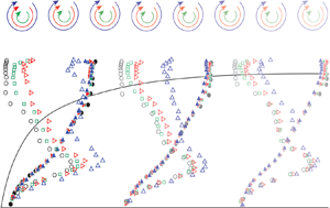
where $x_0$ is a virtual origin, and $A$ and $n$ are the decay coefficient and exponent, respectively. Figure 3 shows the best fits to (3.1), resulting in $n \approx 1$ for all cases. Here, all three variables, $A$, $x_0$ and $n$ were allowed to vary.

Figure 3.

Decay of turbulence for case REF $\bullet$; A $\blacksquare$, green; B $\blacktriangle$, red; C $\blacktriangleright$, blue with fading colours indicating increasing streamwise distance from the grid.

The Taylor microscale in the freestream $\lambda _{\infty }$ was calculated as

(3.2)\begin{equation} \lambda_{\infty}^2 = \frac{{u^{\prime}}^2}{\langle (\partial u / \partial x)^2 \rangle}, \end{equation}

assuming local isotropy and Taylor's frozen flow hypothesis to calculate $(\partial u / \partial x)^2$ from the time series data acquired at a singular streamwise position. A sixth-order central differencing scheme was used to determine the gradients as suggested by Hearst et al. (Reference Hearst, Buxton, Ganapathisubramani and Lavoie2012). This leads to turbulence Reynolds numbers $Re_{\lambda }$ between 45 and 725. A decrease of $Re_{\lambda }$ can be observed both for decreasing $u^{\prime }_0 / U_0$ and with streamwise evolution of the flow, as expected.

The integral length scale $L_{u,\infty }$ was calculated as proposed by Hancock & Bradshaw (Reference Hancock and Bradshaw1989) assuming isotropic turbulence,

(3.3)\begin{equation} U_{\infty} \frac{\mathrm{d}{u^{\prime}_{\infty}}^2}{\mathrm{d}x} = \frac{- ({u^{\prime}_{\infty}}^2)^{3/2}}{L_{u,\infty}}, \end{equation}

where $x$ is the downstream distance from the grid, and the gradient $\mathrm {d}{u^{\prime }_{\infty }}^2 / \mathrm {d}x$ is calculated in physical space by taking the analytical derivative of (3.1). An increase in $L_{u,\infty }$ exists as the distance from the grid grows (table 1), which is expected. The integral scale was also computed by other means, e.g. integrating the auto-correlation to the first zero-crossing, but this approach was found to be less robust. Kozul et al. (Reference Kozul, Hearst, Monty, Ganapathisubramani and Chung2020, figure 7) demonstrated that while the finite value of the integral scale in flows like the present one is dependent on the method chosen for estimating it, the trends with evolution time (distance) and turbulence intensity are preserved.

The global anisotropy is also reported in table 1 as $u^{\prime }_{\infty }/v^{\prime }_{\infty }$. A separate two-component measurement campaign was performed to obtain these estimates. In general, the anisotropy is between 1.1 and 1.2 and thus similar to what is typically reported in grid turbulence (Lavoie et al. Reference Lavoie, Djenidi and Antonia2007) and lower than the anistropy in some other studies of a similar nature (Sharp et al. Reference Sharp, Neuscamman and Warhaft2009; Dogan et al. Reference Dogan, Hearst, Hanson and Ganapathisubramani2019). In most cases, the anistropy grows slightly with downstream distance, which is a result of the slight flow acceleration. Nonetheless, the positional variation in anistropy is always within ${\pm }5\,\%$, which is approximately the uncertainty of this quantity. The isotropy itself was not a controlled parameter, and generally increasing the turbulence intensity with active grids comes with a loss of istropy (Hearst & Lavoie Reference Hearst and Lavoie2015). One should thus consider the present results in light of the anisotropy of the flow, which may also have an influence but was not rigorously controlled.

4. Evolution of the mean and variance profiles

Freestream turbulence has previously been shown to influence turbulent boundary layers all the way down to the wall (Castro Reference Castro1984; Dogan et al. Reference Dogan, Hanson and Ganapathisubramani2016; Hearst et al. Reference Hearst, Dogan and Ganapathisubramani2018). While the majority of earlier studies focused on the influence of FST at a single point, in the present study we demonstrate that the evolution of the FST also plays a significant role. We begin with the mean statistics. In figure 4 the velocity and variance profiles for the four inflow conditions are displayed together for every measurement position, showing the differences between the cases at distinct downstream positions. It can be observed that the velocity profiles all collapse in the viscous sublayer, the buffer layer and the logarithmic region. In the viscous sublayer they follow the relation $U^+ = y^+$, with $U^+$ being a function of the streamwise velocity and the friction velocity $U^+ = U / U_{\tau }$. In the logarithmic region, all profiles agree with the law of the wall. This corresponds to the first three terms in (2.1); the plotted logarithmic region reference line has $\kappa = 0.39$ and $C^+ = 4.35$. The only significant deviation between cases and locations is in the region between the logarithmic layer and the freestream. In a canonical TBL this is the wake region, where large-scale mixing leads to a velocity defect (Coles Reference Coles1956). When subjected to high enough freestream turbulence intensity, the wake region is known to be suppressed (Blair Reference Blair1983a; Thole & Bogard Reference Thole and Bogard1996; Dogan et al. Reference Dogan, Hanson and Ganapathisubramani2016). The freestream, being turbulent itself, leads to a suppression of the intermittent region that typically separates a canonical TBL from an approximately laminar freestream and replaces it with the inherent uniform intermittency of the FST, resulting in a suppressed wake in the boundary layer velocity profile (Dogan et al. Reference Dogan, Hanson and Ganapathisubramani2016). The same can be observed here as presented in figure 4. Case REF with the lowest turbulence intensity of $u^{\prime }_0/U_0 = 3.2\,\%$ shows traces of a wake region at $x/M=35$ which grows with the development of the boundary layer; the wake is visible at $x/M = 55$ and 95. This evolution becomes even more apparent when looking at the velocity profiles of a single case at the three streamwise positions plotted together as presented in figure 5; we note that figure 5 does not contain different information from figure 4, but that plotting it in this way is also informative for comparison. DNS data of a fully developed canonical TBL without FST (Sillero, Jiménez & Moser Reference Sillero, Jiménez and Moser2013) at a $Re_{\tau }$ comparable to REF is included in figure 5 for reference. The mean velocity profile of REF and the DNS are in good agreement at our last measurement station. The variance profiles are roughly in good agreement, but the background turbulence in the freestream elevates the fluctuations in outer regions of the boundary layer for the experiment. At $x/M=95$, the intermediate cases, A and B, also exhibit a wake region in the velocity profile (figures 4c, 5b) with turbulence intensities of $3.8\,\%$ and $5.0\,\%$, respectively, but this is still weaker than the REF case and the DNS. For case B, this trend starts to become visible at $x/M=55$ and $u^{\prime }_{\infty }/U_{\infty } = 4.7\,\%$. This is remarkably consistent with the limit of $u^{\prime }_{\infty }/U_{\infty } = 5.3\,\%$ found by Blair (Reference Blair1983a). The present results demonstrate for the first time that even if the wake region is initially suppressed by the FST, it redevelops as the FST decays below a certain threshold. This is also supported by looking at Coles’ wake parameter ${\varPi }$ (Coles Reference Coles1956). He predicted it to be 0.55 for a canonical turbulent boundary layer with no FST. Marusic et al. (Reference Marusic, McKeon, Monkewitz, Nagib, Smits and Sreenivasan2010) confirmed a similar value in their analysis using the model of Perry, Marusic & Jones (Reference Perry, Marusic and Jones1998). Dogan et al. (Reference Dogan, Hanson and Ganapathisubramani2016) found ${\varPi }=0.55$ in their no-FST case as well and showed that for FST with $7.4\,\% \leqslant u^{\prime }_{\infty }/U_{\infty } \leqslant 12.7\,\%$ at $x/M=43$, Coles’ wake parameter drops to between $-0.52$ and $-0.26$. At $x/M = 35$, the present study shows values between $-0.57$ and $-0.08$ (table 2). For all cases, ${\varPi }$ grows with the development of the TBL. The reference case reaches $\varPi =0.37$, which approaches Coles’ prediction. Both cases A and B eventually reach positive values for the wake parameter as the wake starts to become visible as one moves downstream. Case C does not show a visible recovery of the wake, as illustrated in figure 5(c). A visible difference remains compared to the canonical DNS of Sillero et al. (Reference Sillero, Jiménez and Moser2013). The wake parameter for case C grows but remains negative and within the range of values for FST found by Dogan et al. (Reference Dogan, Hanson and Ganapathisubramani2016) throughout the three positions. $u^{\prime}_{\infty }/U_{\infty }$ does not drop below $7.7\,\%$ within the studied distance from the grid for case C, suggesting it does not drop below the required threshold for wake recovery.

Figure 4.

Mean velocity and variance profiles for cases REF $\bullet$; A $\blacksquare$, green; B $\blacktriangle$, red; C $\blacktriangleright$, blue.

Figure 5.

Development of mean velocity and variance profiles for cases REF $\bullet$; A $\blacksquare$, green and C $\blacktriangleright$, blue with fading colours indicating increasing streamwise distance from the grid. DNS data of a fully developed canonical TBL at $Re_{\tau } \approx 1990$ by Sillero et al. (Reference Sillero, Jiménez and Moser2013) plotted as a reference solid black line.

Table 2.

Boundary layer parameters of the test cases at the different streamwise positions.

In the present study, we define the boundary layer thickness $\delta$ as the point where the velocity reaches $99\,\%$ of the freestream velocity, $\delta = \delta _{99}$. For all cases an increase of the boundary layer thickness is observed with the streamwise evolution of the TBL as documented in table 2. $\delta$ at $x/M = 35$ also scales with $u^{\prime }_{\infty }/U_{\infty }$, likely due to enhanced mixing. It is also worth highlighting that $L_{u,\infty }$ grows with $u^{\prime }_{\infty }/U_{\infty }$ at $x/M = 35$. From the first measurement station, the boundary layers with elevated FST (i.e. cases A, B and C) all grow more rapidly than the REF case.

Freestream turbulence is found to increase the friction velocity $U_{\tau }$ at a given point, in agreement with earlier works (Hancock & Bradshaw Reference Hancock and Bradshaw1989; Blair Reference Blair1983a; Castro Reference Castro1984; Stefes & Fernholz Reference Stefes and Fernholz2004; Dogan et al. Reference Dogan, Hanson and Ganapathisubramani2016; Esteban et al. Reference Esteban, Dogan, Rodríguez-López and Ganapathisubramani2017). This stems from the FST penetrating the boundary layer, increasing mixing and thus the momentum flux towards the wall. This increases the steepness of the velocity profile close to the wall (Dogan et al. Reference Dogan, Hanson and Ganapathisubramani2016) and as a result also the skin friction (Stefes & Fernholz Reference Stefes and Fernholz2004). A decrease in $U_{\tau }$ is observed as the boundary layer develops for each case. This agrees with the behaviour known for spatially evolving canonical turbulent boundary layers without FST (Anderson Reference Anderson2010; Vincenti et al. Reference Vincenti, Klewicki, Morrill-Winter, White and Wosnik2013; Marusic et al. Reference Marusic, Chauhan, Kulandaivelu and Hutchins2015). Values for the friction Reynolds number $Re_{\tau }$ range from 1210 to 5060 and increase both with freestream turbulence intensity and streamwise development. The same is true for $Re_{\theta }$, with values between 3080 and 9050. The empirical parameter $\beta$ defined by Hancock & Bradshaw (Reference Hancock and Bradshaw1989) is included in table 2. It follows the same trends as $u^{\prime }_{\infty }/U_{\infty }$, showing that the influence of the FST is dominant in this flow. Greater discussion of this parameter can be found in appendix C.

The variance profiles at the first measurement positions in figure 4(d) resemble results from Dogan et al. (Reference Dogan, Hanson and Ganapathisubramani2016), Hearst et al. (Reference Hearst, Dogan and Ganapathisubramani2018) and You & Zaki (Reference You and Zaki2019). They showed that the magnitude of the near-wall peak in the variance profiles correlates with the freestream turbulence intensity. The same can be observed in this study. The higher $u^{\prime }_{\infty }/U_{\infty }$, the stronger the near-wall variance peak. FST penetrates the boundary layer and amplifies the fluctuations close to the wall. Moving downstream we can see that the magnitude of the near-wall peaks approach each other until they approximately collapse at $x/M = 95$ (figure 4f). Note that the four flows all still have distinct $u^{\prime }_{\infty }/U_{\infty }$, $L_{u,\infty }$ and $\delta$ at $x/M = 95$. Thus, the present results demonstrate that if the boundary layer is allowed to evolve for a sufficient time, the correlation between the FST magnitude and the near-wall variance peak magnitude diminishes. This differs from earlier measurements performed at a single downstream position that could not observe this phenomenon. Taking a closer look at the development of the near-wall peak for the cases REF, A and C in figure 5, it becomes apparent that the approach to a common near-wall variance peak magnitude is due to different underlying trends in the four cases. For REF, the near-wall variance peak steadily increases with downstream position. This is in agreement with the results from Marusic et al. (Reference Marusic, Chauhan, Kulandaivelu and Hutchins2015) for spatially evolving canonical TBLs without FST. This trend is diminished but still present for case A; case B is similar to case A and is not plotted to reduce clutter. For case C, with the highest initial turbulence intensity, the trend reverses: instead of an increase, the near-wall variance peak decreases significantly with the development of the boundary layer. It can be concluded that the spatial development of the near-wall variance peak is strongly dependent on the initial level of turbulence intensity but approaches a common value downstream independently of the initial freestream state, at least for a given $Re_{\tau }$. Hutchins & Marusic (Reference Hutchins and Marusic2007) predicted this to be between 8.4 and 9.2 for the $Re_{\tau }$ examined here. The present measurements find a similar value of ${u^{\prime }}^2/U_{\tau }^2 \approx 9.5$. This is slightly higher than what was found by Hutchins & Marusic (Reference Hutchins and Marusic2007), which could be a result of the remaining freestream turbulence still present at the last measurement position, or differences in the noise floors of the measurement techniques used.

The displacement thickness $\delta ^*= \int _0^{\infty }(1-U(y)/U_{\infty })\,\mathrm {d}y$ and momentum thickness $\theta =\int _0^{\infty } U(y)/U_{\infty } (1-U(y)/U_{\infty })\,\mathrm {d}y$ grow with streamwise evolution for all cases. The ratio between the two is the shape factor $H = \delta ^*/\theta$, which is an indicator of the fullness of the boundary layer profile. Small deviations for the dimensional quantities $\delta ^*$ and $\theta$ can be explained by differences in the mean velocity and uncertainty in the measurements. The trend is still captured accurately. Consequently, in the nondimensional $H$, the small deviations vanish. This study shows that freestream turbulence reduces the shape factor as the boundary layer profile becomes fuller – i.e. the velocity rises more steeply close to the wall, while farther away from the wall the velocity profile becomes flatter. This is in good agreement with previous studies (Hancock & Bradshaw Reference Hancock and Bradshaw1983; Castro Reference Castro1984; Stefes & Fernholz Reference Stefes and Fernholz2004; Dogan et al. Reference Dogan, Hanson and Ganapathisubramani2016; Hearst et al. Reference Hearst, Dogan and Ganapathisubramani2018). As presented in figure 6 and table 2, the higher the initial turbulence intensity, the lower the shape factor. For a canonical turbulent boundary layer, Monkewitz, Chauhan & Nagib (Reference Monkewitz, Chauhan and Nagib2008) found that the shape factor decreases with increasing $Re_{\theta }$. This is confirmed for each downstream position in this study as depicted in figure 6; the data from Dogan et al. (Reference Dogan, Hanson and Ganapathisubramani2016) have also been plotted showing the same trend.

Figure 6.

Development of the shape factor $H$ for cases REF $\bullet$; A $\blacksquare$, green; B $\blacktriangle$, red; C $\blacktriangleright$, blue with fading colours indicating increasing streamwise distance from the grid. The data of Hancock & Bradshaw (Reference Hancock and Bradshaw1983) $\square$ and Dogan et al. (Reference Dogan, Hanson and Ganapathisubramani2016) $\circ$ are also included for reference. Lines connecting points indicate that they were acquired from the same set-up but at different streamwise positions. All Dogan et al. (Reference Dogan, Hanson and Ganapathisubramani2016) measurements were conducted at the same location but with different freestream conditions.

The aforementioned trend pertains to a single position. However, the question of how the evolution of $H$ is impacted by the FST is still open. The data of Hancock & Bradshaw (Reference Hancock and Bradshaw1983) suggest a decrease of the shape factor as one moves downstream; this data is also included in figure 6. It has to be kept in mind that their measurements were for relatively low turbulence intensities, and some of them were very close to the grid. We show that when the turbulence intensity in the freestream is increased further and the measurements are taken past $x/M=30$, this trend reverses. The shape factor is reduced significantly at the first measurement position, and as the freestream turbulence decreases it recovers towards its natural value. This value can be obtained by looking at the shape factor of canonical zero pressure gradient turbulent boundary layers for a wide range of $Re_{\delta ^*}=U_{\infty } \delta ^* / \nu$ as presented by Chauhan et al. (Reference Chauhan, Monkewitz and Nagib2009). For $Re_{\delta ^*}$ between 4000 and 10 000, as found in the present study, a shape factor between 1.35 and 1.41 would be expected without the presence of freestream turbulence (Chauhan et al. Reference Chauhan, Monkewitz and Nagib2009). While the shape factors of Hancock & Bradshaw (Reference Hancock and Bradshaw1983) drop away from the canonical values with increasing distance from the grid (Chauhan et al. Reference Chauhan, Monkewitz and Nagib2009), the data presented herein trend toward the predicted values. The boundary layer appears to forget it started with different conditions as the influence of these conditions diminishes farther downstream.

The continuous streamwise development of the boundary layer results in an increase of $Re_{\tau }$ for all cases. At the same time $Re_{\tau }$ scales with the level of freestream turbulence which decays with streamwise evolution of the flow. It is therefore interesting to compare boundary layers with similar $Re_{\tau }$ but different paths to get there. This is done in figure 7 with the reference case at $x/M=95$ with $u^{\prime }_{\infty }/U_{\infty } = 2.5\,\%$ and $Re_{\tau }=1870$ and case A at $x/M=35$ with $u^{\prime }_{\infty }/U_{\infty } = 5.5\,\%$ and $Re_{\tau }=1990$ (figure 7a,c), as well as with case A at $x/M=95$ with $u^{\prime }_{\infty }/U_{\infty } = 3.8\,\%$ and $Re_{\tau }=3700$ and case C at $x/M=35$ with $u^{\prime }_{\infty }/U_{\infty } = 12.5\,\%$ and $Re_{\tau }=3610$ (figure 7b,d). For the first comparison (figure 7a,c) with a moderate difference in freestream turbulence intensity, the deviations in the variance profiles are small. Nevertheless, a distinction in the outer region is visible in the velocity profile. Whereas for case A at $x/M=35$ the wake is still suppressed, for the most part, the reference case at $x/M=95$ displays a pronounced wake region. This is particularly interesting given these two cases have essentially the same freestream integral scale, $L_{u,\infty } \approx 310\ \textrm {mm}$ and $2.1 \le L_{u,\infty }/\delta \le 2.3$, suggesting that this parameter is not what is driving the difference in the outer region. When comparing cases with a bigger difference in freestream turbulence (figure 7b,d), the differences become even more distinct. Once again the velocity profiles are collapsed in the viscous sublayer, the buffer layer and the logarithmic region. Farther away from the wall the profiles diverge. For case C the wake region is fully suppressed at this point, whereas case A at $x/M=95$ shows the reemergence of a wake. In the variance profiles the considerable difference in $u^{\prime }_{\infty }/U_{\infty }$ is visible. Moving closer to the wall it becomes evident that the turbulence intensity in the freestream also influences the boundary layer close to the wall. The near-wall variance peak is significantly more pronounced for the case with the higher freestream turbulence intensity. These particular cases have the same $L_{u,\infty }$ and $1.9 \le L_{u,\infty }/\delta \le 2.0$, again suggesting the above differences are not a result of a difference in the size of the large scales in the freestream. The same general trends were also observed at $Re_{\tau } \approx 4500$. One can thus conclude that $Re_{\tau }$ alone is not sufficient to describe the profile of a turbulent boundary layer subjected to FST, but rather $u^{\prime }_{\infty }/U_{\infty }$ and the evolution distance must also be considered at a minimum.

Figure 7.

Comparison of TBL profiles with similar $Re_{\tau }$: (a,c) case REF at $x/M=95$ $\bullet$, grey and case A at $x/M=35$ $\blacksquare$, green; (b,d) case A at $x/M=95$ $\blacksquare$, light green and case C at $x/M=35$ $\blacktriangleright$, blue.

5. Evolution of the spectral distribution of energy

Further insight into the processes governing the evolution of a TBL subjected to FST can be gained by looking at the spectral distribution of energy at different streamwise positions. For this, the pre-multiplied spectra, $\phi ^+ = k_x \phi _u / U_{\tau }^2$, at every wall-normal position are plotted together in a contour map illustrating regions and wavelengths, $\zeta ^+ = 2 {\rm \pi}U_{\tau } / k_x \nu$, with high and low energy. This is based on the streamwise energy spectra $\phi _u$ in normalized wavenumber space $k_x$. Computing spectra from the LDV measurements is not as straightforward as it is from hot-wires, which is the more common measurement technique in TBLs. As stated in § 2, we have used the sample and hold technique to compute the spectra and applied a bandwidth moving filter. The spectra are also computed over less boundary layer turn-overs than is typical in hot-wire measurements, despite the long sample times used herein. As such, we provide the present spectra as qualitative relative comparisons in which we have confidence, rather than exact quantitative comparisons to the hot-wire-acquired spectra in the literature.

Hutchins & Marusic (Reference Hutchins and Marusic2007) showed that in a canonical turbulent boundary layer there is a fixed peak close to the wall at $y^+ \approx 15$ and $\zeta ^+ \approx 1000$. They further showed that for high $Re_{\tau } = 7300$, an outer spectral peak emerges. The evolution of the spectrograms in a spatially developing TBL for different initial freestream turbulence intensities is presented in figure 8. The first observation is that in agreement with Dogan et al. (Reference Dogan, Hanson and Ganapathisubramani2016), Hearst et al. (Reference Hearst, Dogan and Ganapathisubramani2018) and Ganapathisubramani (Reference Ganapathisubramani2018), the location of the near-wall spectral peak is independent of the level of freestream turbulence and coincides with the location found by Hutchins & Marusic (Reference Hutchins and Marusic2007). It seems that the small scales close to the wall are not affected by the freestream turbulence. This is displayed explicitly in figure 9, where the larger scales deviate visibly for the higher FST cases above $u^{\prime }_{\infty }/U_{\infty } \approx 6\,\%$, in agreement with Hearst et al. (Reference Hearst, Dogan and Ganapathisubramani2018).

Figure 8.

Spectrograms for cases REF (a–c), A (d–f), B (g–i) and C (j–l) at the three streamwise positions with increasing level of freestream turbulence from top to bottom.

Figure 9.

Normalized pre-multiplied velocity spectra at the near-wall spectral peak for cases REF solid black line, A solid green line, B solid red line, C solid blue with fading colours indicating increasing streamwise distance from the grid.

Looking at the first measurement position, $x/M = 35$, in figure 8 confirms the findings of Sharp et al. (Reference Sharp, Neuscamman and Warhaft2009), Dogan et al. (Reference Dogan, Hanson and Ganapathisubramani2016) and Hearst et al. (Reference Hearst, Dogan and Ganapathisubramani2018) that when subjected to strong enough FST an outer spectral peak forms at considerably lower Reynolds numbers than in canonical TBLs – here at $Re_{\tau }=3610$ for case C. For the lowest $Re_{\tau }$ of 1210, corresponding to the reference case at $x/M = 35$, no outer peak exists, and the spectrogram resembles the shape found by Hutchins & Marusic (Reference Hutchins and Marusic2007) for $Re_{\tau }=1010$. Cases B and C at $x/M=35$ demonstrate a timid emergence of an outer spectral peak. The novel element of the present study is the streamwise development of these features. For cases REF, A and B, with initial turbulence intensities between $3.2\,\%$ and $7.4\,\%$, the outer spectral peak grows in magnitude and moves away from the wall as the boundary layer develops. Of these three cases, case B with the highest initial turbulence intensity $u^{\prime }_0/U_0$, shows the strongest outer spectral peak. This agrees with the trend for increasing $Re_{\tau }$ detected by Hutchins & Marusic (Reference Hutchins and Marusic2007) in a canonical TBL.

Up until the present study there has been no reason not to expect a growth of the outer spectral peak with increasing $Re_{\tau }$ for higher freestream turbulence intensities as well. Instead, case C with the highest initial turbulence intensity of $u^{\prime }_0 / U_0 = 12.5\,\%$, presents different behaviour. The outer spectral peak is pronounced at $x/M=35$. In contrast to the expected continuous growth of the outer spectral peak in canonical TBLs, here it gradually decreases as the boundary layer develops and the freestream turbulence decays. Thus, if one did not know the measured values of $Re_{\tau }$, the spectrogram from earlier in the spatial evolution of case C gives the impression it is at a higher $Re_{\tau }$ than those from farther downstream. In contrast to the lower FST cases, the decay of the freestream turbulence more significantly influences the spectrogram than the growth of the TBL. This fading of the outer spectral peak is visible throughout the three measurement positions for case C. This behavior becomes more evident when looking at the net change $\Delta ^+ = (\phi ^+ - \phi ^+_0) / \phi ^+_{0,max}$ in spectrograms, where $\phi ^+_0$ is the spectrogram at $x/M=35$. This is displayed in figure 10 for the reference case compared to case C with the highest freestream turbulence intensity. The reference case (figure 10a,b) shows the slow emergence of an outer peak with a positive net change $\Delta ^+$ for $\zeta ^+ \approx 10^4$ most distinctly in the outer regions of the boundary layer at $y^+ \approx 10^3$. The opposite is observed for case C in figure 10(c,d), with a negative net change where the outer spectral peak was initially most pronounced at $10^3 \lesssim y^+ \lesssim 10^4$ and $10^4 \lesssim \zeta ^+ \lesssim 10^5$. The location of the outer spectral peak in outer scaling, i.e. $y/\delta$ and $\zeta /\delta$, does not coincide with the location for canonical TBLs identified by Hutchins & Marusic (Reference Hutchins and Marusic2007). This is to be expected for a TBL subjected to FST (Dogan et al. Reference Dogan, Hanson and Ganapathisubramani2016; Hearst et al. Reference Hearst, Dogan and Ganapathisubramani2018). The reason for this is that the peak is superimposed onto the outer boundary layer by the freestream turbulence. In fact, the peak is situated much higher for the FST cases and moves only once the boundary layer starts to redistribute the energy. This is documented in great detail for numerous cases in Hearst et al. (Reference Hearst, Dogan and Ganapathisubramani2018). As the outer peak evolves in this study, it approaches $\zeta _x/\delta \approx 10$ and $y/\delta \approx 0.4$ as found by Hearst et al. (Reference Hearst, Dogan and Ganapathisubramani2018).

Figure 10.

Net change $\Delta ^+ = (\phi ^+ - \phi ^+_0) / \phi ^+_{0,max}$ in spectrograms at $x/M=55$ and $x/M=95$ for cases REF (a,b) and C (c,d) with respect to initial spectrogram at $x/M=35$. The contour lines of the initial spectrogram are imprinted as a reference.

It is also interesting to compare case B at $x/M=35$ (figure 8g) and case C at $x/M=95$ (figure 8l), which have approximately the same freestream turbulence intensity $7.4\,\% \le u^{\prime }_{\infty } / U_{\infty }\le 7.7\,\%$ and integral scale relative to the boundary layer thickness $2.6 \le L_{u,\infty }/\delta \le 2.7$. Their spectrograms look very different, demonstrating the importance of the evolution on the energy distribution within the boundary layer. Furthermore, when comparing cases with similar $Re_{\tau }$, e.g. case A at $x/M=95$ (figure 8f) and case C at $x/M=35$ (figure 8j), the difference is even more apparent. Figure 8(f) shows a hint of an outer spectral peak, while figure 8(j) represents the most prominent occurrence of an outer peak of all the measurements. This underlines the fact that $Re_{\tau }$ must be considered alongside $u^{\prime }_{\infty } / U_{\infty }$ and the evolution distance when studying TBLs subjected to FST.

6. Global trends

The way this experiment was constituted, there were two main factors modulating the boundary layer contrarily to each other. On the one hand, the TBL was evolving spatially, growing and becoming more developed. On the other hand, the FST, which artificially matured the state of evolution of the boundary layer, decayed with increasing distance $x$ from its origin, the active grid. The streamwise evolution of a boundary layer may be expressed through $Re_x = U_{\infty } x / \nu$. Figure 11 summarizes how the natural growth of the boundary layer and the decay of the freestream turbulence interact, and which prevails under what conditions. The implications for different characteristics of a TBL are examined as the boundary layers evolve spatially.

Figure 11.

Trends for an evolving turbulent boundary layer subjected to different levels of freestream turbulence. Case REF $\bullet$; A $\blacksquare$, green; B $\blacktriangle$, red; C $\blacktriangleright$, blue with fading colours indicating increasing streamwise distance from the grid.

The boundary layer at a single position thickens with increasing freestream turbulence intensity. As the flow evolves, the turbulence in the freestream decays and the integral scale grows. At the same time the boundary layer develops. Overall this leads to a growth of the boundary layer thickness for all levels of freestream turbulence. Figure 11(b) shows a relatively uniform stacking of the boundary layer thickness with $u^{\prime }_{\infty }/U_{\infty }$ for low $Re_x$. As the flow develops, the higher FST intensity cases A, B and C have similar values of $\delta$, while $\delta$ for REF is demonstrably smaller. The influence of $u^{\prime }_{\infty } / U_{\infty }$ on $\delta$ decreases as the flow evolves, but a distinct difference remains between low and moderate to high FST intensity.

For a sufficiently developed canonical turbulent boundary layer, the shape factor $H$ decreases with increasing $Re_x$ (Vincenti et al. Reference Vincenti, Klewicki, Morrill-Winter, White and Wosnik2013; Marusic et al. Reference Marusic, Chauhan, Kulandaivelu and Hutchins2015). This decrease can also be achieved by introducing FST in the flow. The result is, contrarily to a canonical TBL, $H$ grows with increasing $Re_x$ as the boundary layer develops beneath decaying FST. Presumably there is a turning point when $H$ will start decreasing again. Throughout the examined range, the shape factor remains distinguished by $u^{\prime }_{\infty } / U_{\infty }$ (figure 11c). The influence of the initial difference in freestream turbulence is transported through the examined range of $Re_x$. Similar behaviour can be observed for the wake region of the TBL. This is quantified through Coles’ wake parameter ${\varPi }$, which is known to trend towards a fixed value for canonical conditions with high Reynolds numbers and sufficient development length (Marusic et al. Reference Marusic, McKeon, Monkewitz, Nagib, Smits and Sreenivasan2010). Freestream turbulence suppresses the intermittency in the wake region, thus leading to the suppression of the typical flow profile seen in the wake region and a significantly depleted wake parameter (Dogan et al. Reference Dogan, Hanson and Ganapathisubramani2016). The stronger the freestream turbulence intensity, the lower ${\varPi }$ becomes. The wake is predominantly influenced by the FST, and as it decays, the wake becomes more pronounced. The overall change of $\varPi$ with spatial evolution is more substantial than the change to $H$. For the lower turbulence intensities, $\varPi$ approaches the analytical value of 0.55 (Coles Reference Coles1956), and a visible wake region re-emerges within the investigated spatial development range (figure 5). The change in shape of the boundary layer indicates that the FST penetrates the boundary layer and has an influence on its evolution.

How deep and how significant that influence is becomes evident when looking at the modulation of the near-wall variance peak at $y^+ \approx 15$. The magnitude is strongly dependent on the level of turbulence in the freestream, with a higher turbulence intensity correlating with a higher peak in the variance. For canonical TBLs, the near-wall peak increases with the evolution of the boundary layer until the profiles become self-similar. This behaviour can be observed for lower initial freestream turbulence up to ${u^{\prime }_0/U_0=5.5\,\%}$. For the highest freestream turbulence intensity, the decay of the turbulence proves to be dominant, as the near-wall variance peak decreases in magnitude as the flow evolves.

For high enough $Re_{\tau }$, TBLs develop an outer peak in the spectral energy distribution (Hutchins & Marusic Reference Hutchins and Marusic2007). This state can also be reached by subjecting the boundary layer to high-intensity freestream turbulence (Dogan et al. Reference Dogan, Hanson and Ganapathisubramani2016; Hearst et al. Reference Hearst, Dogan and Ganapathisubramani2018). For canonical TBLs, this peak develops as the boundary layer grows spatially and $Re_{\tau }$ increases. This is observed for the lower freestream turbulence cases $3.2\,\% \leqslant u^{\prime }_0/U_0 \leqslant 7.4\,\%$ here. Initially there is no outer peak visible in the spectrograms, but as the boundary layer develops, the magnitude of the outer peak gradually increases. This evolution looks very different for the highest level of freestream turbulence. A strong peak exists at the first measurement position, then proceeds to decrease with streamwise evolution of the flow. For this case, the decay of the FST appears to drive the phenomenology. The drop in outer peak magnitude is significantly higher than the observed increase for the lower FST cases (figure 11f). We thus again arrive at the conclusion that these flows must be parameterized by $Re_{\tau }$, $u^{\prime }_{\infty } / U_{\infty }$ and the streamwise development of the flow.