


Impact Statement
A stochastic VAE-based data-driven model pre-trained on imperfect climate simulations and re-trained with transfer learning, on a limited number of observations, leads to accurate short-term weather forecasting along with long-term stable non-drifting climate.
1. Introduction
A surge of interest in building deep learning-based data-driven models for complex systems such as chaotic dynamical systems (Pathak et al., Reference Pathak, Hunt, Girvan, Lu and Ott2018; Chattopadhyay et al., Reference Chattopadhyay, Hassanzadeh and Subramanian2020a), fully turbulent flow (Chattopadhyay et al., Reference Chattopadhyay, Mustafa, Hassanzadeh and Kashinath2020b), and weather and climate models (Weyn et al., Reference Weyn, Durran and Caruana2019, Reference Weyn, Durran and Caruana2020, Reference Weyn, Durran, Caruana and Cresswell-Clay2021; Rasp and Thuerey, Reference Rasp and Thuerey2021; Chattopadhyay et al., Reference Chattopadhyay, Mustafa, Hassanzadeh, Bach and Kashinath2022) has been seen in the recent past. This interest in data-driven modeling stems from the hope that if these data-driven models are trained on observational data, (a) they would not suffer from some of the biases of physics-based numerical climate and weather models (Balaji, Reference Balaji2021; Schultz et al., Reference Schultz, Betancourt, Gong, Kleinert, Langguth, Leufen, Mozaffari and Stadtler2021), for example, due to ad hoc parameterizations, (b) they can be used to generate large ensemble forecasts for data assimilation (Chattopadhyay et al., Reference Chattopadhyay, Mustafa, Hassanzadeh, Bach and Kashinath2022), and (c) they might seamlessly be integrated to perform climate simulations (Watson-Parris, Reference Watson-Parris2021) that would allow for generating large synthetic datasets to study extreme events (Chattopadhyay et al., Reference Chattopadhyay, Nabizadeh and Hassanzadeh2020c).
Despite the promise of data-driven weather prediction (DDWP) models, most DDWP models cannot compete with state-of-the-art numerical weather prediction (NWP) models (Scher and Messori, Reference Scher and Messori2019; Weyn et al., Reference Weyn, Durran and Caruana2019, Reference Weyn, Durran and Caruana2020; Rasp and Thuerey, Reference Rasp and Thuerey2021; Chattopadhyay et al., Reference Chattopadhyay, Mustafa, Hassanzadeh, Bach and Kashinath2022) although more recently FourCastNet (Pathak et al., Reference Pathak, Subramanian, Harrington, Raja, Chattopadhyay, Mardani, Kurth, Hall, Li, Azizzadenesheli, Hassanzadeh, Kashinath and Anandkumar2022) has shown promise of being quite competitive with the best NWP models. There have also been some previous works, where pre-training models on climate simulations have also resulted in improved short-term forecasts on reanalysis datasets (Rasp and Thuerey, Reference Rasp and Thuerey2021). Moreover, these DDWP models, while comparable with NWP in terms of short-term forecasts, are unstable when integrated for longer time scales. These instabilities either appear in the form of blow-ups or unphysical climate drifts (Scher and Messori, Reference Scher and Messori2019; Chattopadhyay et al., Reference Chattopadhyay, Mustafa, Hassanzadeh and Kashinath2020b).
In this article, we consider the following realistic problem set-up, wherein, we have long-term climate simulations from an imperfect two-layer quasi-geostrophic (QG) flow (we will call it “imperfect system” hereafter) at our disposal to pre-train a DDWP. Following that, we have a few noisy observations from a perfect two-layer QG flow (“perfect system” hereafter) on which we are able to fine-tune our DDWP. This observationally constrained DDWP model is then expected to generalize to the perfect system with a noisy initial condition (obtained from the available observations) and perform stochastic short-term forecasting. It is also expected to be seamlessly time-integrated to obtain long-term climatology. We show that in this regard, a stochastic forecasting approach with a generative model such as a convolutional variational autoencoder (VAE) outperforms a deterministic encoder–decoder-based convolutional architecture in terms of short-term forecasts and remains stable without unphysical climate drift for long-term integration. A deterministic encoder–decoder would fail to do so and shows unphysical climate drift followed by a numerical blow-up.
2. Methods
2.1. Imperfect and perfect systems
In this article, we consider two-layer QG flow as the geophysical system on which we intend to perform both short-term forecasting and compute long-term statistics.
The dimensionless dynamical equations of the two-layer QG flow are derived following Lutsko et al. (Reference Lutsko, Held and Zurita-Gotor2015) and Nabizadeh et al. (Reference Nabizadeh, Hassanzadeh, Yang and Barnes2019). The system consists of two constant density layers with a $ \beta $
-plane approximation in which the meridional temperature gradient is relaxed toward an equilibrium profile. The equation of the system is described as
$ \beta $
-plane approximation in which the meridional temperature gradient is relaxed toward an equilibrium profile. The equation of the system is described as
 $$ {\displaystyle \begin{array}{l}\frac{\partial {q}_j}{\partial t}+J\left({\psi}_j,{q}_j\right)\hskip0.35em =\hskip0.35em -\frac{1}{\tau_d}{\left(-1\right)}^j\left({\psi}_1-{\psi}_2-{\psi}_R\right)\\ {}\hskip11.6em -\frac{1}{\tau_f}{\delta}_{k2}{\nabla}^2{\psi}_j-\nu {\nabla}^8{q}_j.\end{array}} $$
Here, $ q $
is potential vorticity and is expressed as
$ q $
is potential vorticity and is expressed as
 $$ {q}_j\hskip0.35em =\hskip0.35em {\nabla}^2{\psi}_j+{\left(-1\right)}^j\left({\psi}_1-{\psi}_2\right)+\beta y, $$
where $ {\psi}_j $
is the stream function of the system. In Equations (1) and (2),
$ {\psi}_j $
is the stream function of the system. In Equations (1) and (2), $ j $
denotes the upper (
$ j $
denotes the upper ( $ j\hskip0.35em =\hskip0.35em 1 $
) and lower (
$ j\hskip0.35em =\hskip0.35em 1 $
) and lower ( $ j\hskip0.35em =\hskip0.35em 2 $
) layers.
$ j\hskip0.35em =\hskip0.35em 2 $
) layers. $ {\tau}_d $
is the Newtonian relaxation time scale while
$ {\tau}_d $
is the Newtonian relaxation time scale while $ {\tau}_f $
is the Rayleigh friction time scale, which only acts on the lower layers represented by the Kronecker
$ {\tau}_f $
is the Rayleigh friction time scale, which only acts on the lower layers represented by the Kronecker $ \delta $
function (
$ \delta $
function ( $ {\delta}_{k2} $
).
$ {\delta}_{k2} $
). $ J $
denotes the Jacobian,
$ J $
denotes the Jacobian, $ \beta $
is the
$ \beta $
is the $ y- $
gradient of the Coriolis parameter, and
$ y- $
gradient of the Coriolis parameter, and $ \nu $
denotes the hyperdiffusion coefficient. We have induced a baroclinically unstable jet at the center of a horizontally (zonally) periodic channel by setting
$ \nu $
denotes the hyperdiffusion coefficient. We have induced a baroclinically unstable jet at the center of a horizontally (zonally) periodic channel by setting $ {\psi}_1-{\psi}_2 $
to be equal to a hyperbolic secant centered at
$ {\psi}_1-{\psi}_2 $
to be equal to a hyperbolic secant centered at $ y\hskip0.35em =\hskip0.35em 0 $
. When eddy fluxes are absent,
$ y\hskip0.35em =\hskip0.35em 0 $
. When eddy fluxes are absent, $ {\psi}_2 $
is identically zero, making zonal velocity in the upper layer
$ {\psi}_2 $
is identically zero, making zonal velocity in the upper layer $ u(y)\hskip0.35em =\hskip0.35em -\frac{\partial {\psi}_1}{\partial y}\hskip0.35em =\hskip0.35em -\frac{\partial {\psi}_R}{\partial y} $
where we set
$ u(y)\hskip0.35em =\hskip0.35em -\frac{\partial {\psi}_1}{\partial y}\hskip0.35em =\hskip0.35em -\frac{\partial {\psi}_R}{\partial y} $
where we set
 $$ -\frac{\partial {\psi}_R}{\partial y}\hskip0.35em =\hskip0.35em {\operatorname{sech}}^2\left(\frac{y}{\sigma}\right), $$ $ \sigma $
being the width of the jet. Parameters of the model are set following the previous studies (Lutsko et al., Reference Lutsko, Held and Zurita-Gotor2015; Nabizadeh et al., Reference Nabizadeh, Hassanzadeh, Yang and Barnes2019), in which
$ \sigma $
being the width of the jet. Parameters of the model are set following the previous studies (Lutsko et al., Reference Lutsko, Held and Zurita-Gotor2015; Nabizadeh et al., Reference Nabizadeh, Hassanzadeh, Yang and Barnes2019), in which $ \beta \hskip0.35em =\hskip0.35em 0.19 $
,
$ \beta \hskip0.35em =\hskip0.35em 0.19 $
, $ \sigma \hskip0.35em =\hskip0.35em 3.5 $
,
$ \sigma \hskip0.35em =\hskip0.35em 3.5 $
, $ {\tau}_f\hskip0.35em =\hskip0.35em 15 $
, and
$ {\tau}_f\hskip0.35em =\hskip0.35em 15 $
, and $ {\tau}_d\hskip0.35em =\hskip0.35em 100 $
.
$ {\tau}_d\hskip0.35em =\hskip0.35em 100 $
.
To non-dimensionalize the equations, we have used the maximum strength of the equilibrium velocity profile as the velocity scale ( $ U $
) and the deformation radius (
$ U $
) and the deformation radius ( $ L $
) for the length scale. The system’s time scale (
$ L $
) for the length scale. The system’s time scale ( $ L/U $
) is referred to as the “advective time scale” (
$ L/U $
) is referred to as the “advective time scale” ( $ {\tau}_{adv} $
).
$ {\tau}_{adv} $
).
The spatial discretization is spectral in both $ x $
and
$ x $
and $ y $
where we have retained 96 and 192 Fourier modes, respectively. The length and width of the domain is equal to 46 and 68, respectively, after non-dimensionalizing the numbers. The spurious waves on the northern and southern boundaries are damped by applying sponge layers. Note that, the domain is wide enough that the sponges do not affect the dynamics. Here,
$ y $
where we have retained 96 and 192 Fourier modes, respectively. The length and width of the domain is equal to 46 and 68, respectively, after non-dimensionalizing the numbers. The spurious waves on the northern and southern boundaries are damped by applying sponge layers. Note that, the domain is wide enough that the sponges do not affect the dynamics. Here, $ 5{\tau}_{adv}\hskip0.35em \approx \hskip0.35em 1 $
Earth day
$ 5{\tau}_{adv}\hskip0.35em \approx \hskip0.35em 1 $
Earth day $ \approx \hskip0.35em 200\Delta {t}_n $
, where
$ \approx \hskip0.35em 200\Delta {t}_n $
, where $ \Delta {t}_n\hskip0.35em =\hskip0.35em 0.025 $
is the time step of the leapfrog time integrator used in the numerical scheme.
$ \Delta {t}_n\hskip0.35em =\hskip0.35em 0.025 $
is the time step of the leapfrog time integrator used in the numerical scheme.
The imperfect system in this article has an increased value of $ \beta $
, given by
$ \beta $
, given by $ {\beta}^{\ast}\hskip0.35em =\hskip0.35em 3\beta $
and a decreased size of the jet, given by
$ {\beta}^{\ast}\hskip0.35em =\hskip0.35em 3\beta $
and a decreased size of the jet, given by $ \sigma \ast \hskip0.35em =\hskip0.35em \frac{4}{5}\sigma $
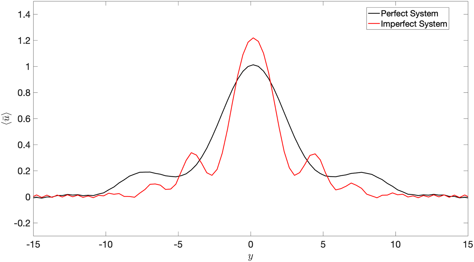
. We assume that we have long-term climate simulations of the imperfect system while we have only a few noisy observations of the perfect system. The difference in the long-term averaged zonal-mean velocity in the upper layer of the perfect and imperfect systems is shown in Figure 1. It is to be noted that the motivation behind having an imperfect and perfect system is the fact that we assume that the imperfect system represents a climate model with biases from which we have long simulations at our disposal, whereas the perfect system is analogous to actual observations from our atmosphere, where the sample size is small and contaminated with measurement noise.
$ \sigma \ast \hskip0.35em =\hskip0.35em \frac{4}{5}\sigma $
. We assume that we have long-term climate simulations of the imperfect system while we have only a few noisy observations of the perfect system. The difference in the long-term averaged zonal-mean velocity in the upper layer of the perfect and imperfect systems is shown in Figure 1. It is to be noted that the motivation behind having an imperfect and perfect system is the fact that we assume that the imperfect system represents a climate model with biases from which we have long simulations at our disposal, whereas the perfect system is analogous to actual observations from our atmosphere, where the sample size is small and contaminated with measurement noise.
Time-averaged zonal-mean velocity (over 20,000 days), $ \left\langle \overline{u}\right\rangle $
, of the imperfect and perfect system. The difference between
$ \left\langle \overline{u}\right\rangle $
, of the imperfect and perfect system. The difference between $ \left\langle \overline{u}\right\rangle $
of the perfect and imperfect systems indicates a challenge for DDWP models to seamlessly generalize from one system to the other.
$ \left\langle \overline{u}\right\rangle $
of the perfect and imperfect systems indicates a challenge for DDWP models to seamlessly generalize from one system to the other.
2.2. VAE and transfer learning frameworks
Here, we propose a generative modeling approach to perform both short- and long-term forecasting for the perfect QG system after being trained on the imperfect QG system. We assume that we have a long-term climate simulation from the imperfect system, with states $ {x}^m\left(k\Delta t\right) $
, where
$ {x}^m\left(k\Delta t\right) $
, where $ k\in 1,\hskip0.35em 2,\cdots K $
and
$ k\in 1,\hskip0.35em 2,\cdots K $
and $ {x}^m\in {\mathrm{\mathcal{R}}}^{2\times 96\times 192} $
. A convolutional VAE is trained on the states of this imperfect system to predict an ensemble of states with a probability density function,
$ {x}^m\in {\mathrm{\mathcal{R}}}^{2\times 96\times 192} $
. A convolutional VAE is trained on the states of this imperfect system to predict an ensemble of states with a probability density function, $ p\left({x}^m\left(t+\Delta t\right)\right) $
, from
$ p\left({x}^m\left(t+\Delta t\right)\right) $
, from $ {x}^m(t) $
. Here,
$ {x}^m(t) $
. Here, $ \Delta t\hskip0.35em =\hskip0.35em 40\Delta {t}_n $
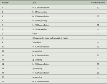
, which is also the sampling interval for training the model. Extensive trial and error-based search has been performed for hyperparameter optimization for the VAE. The details on the VAE architecture are given in Table 1.
$ \Delta t\hskip0.35em =\hskip0.35em 40\Delta {t}_n $
, which is also the sampling interval for training the model. Extensive trial and error-based search has been performed for hyperparameter optimization for the VAE. The details on the VAE architecture are given in Table 1.
Number of layers and filters in the convolutional VAE architecture used in this article.
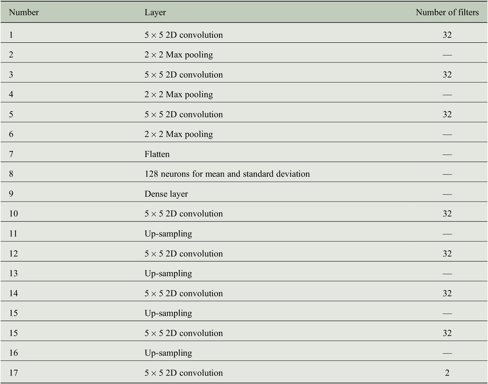
Note. The baseline convolutional encoder–decoder model would have the exact same architecture and the same latent space size as that of the VAE.
This pre-trained VAE would then undergo transfer learning on a small number of noisy observations of the states of the perfect system $ {x}^o\left(n\Delta t\right) $
, where
$ {x}^o\left(n\Delta t\right) $
, where $ n\in 1,\hskip0.35em 2,\cdots N $
and
$ n\in 1,\hskip0.35em 2,\cdots N $
and $ N\hskip0.35em \ll \hskip0.35em K $
. The VAE would then stochastically forecast an ensemble of states of the perfect system with a noisy initial condition from the perfect system. The noise in the initial condition is sampled from a Gaussian normal distribution with 0 mean and standard deviation being
$ N\hskip0.35em \ll \hskip0.35em K $
. The VAE would then stochastically forecast an ensemble of states of the perfect system with a noisy initial condition from the perfect system. The noise in the initial condition is sampled from a Gaussian normal distribution with 0 mean and standard deviation being $ {\eta \sigma}_Z $
, where
$ {\eta \sigma}_Z $
, where $ {\sigma}_Z $
is the standard deviation of
$ {\sigma}_Z $
is the standard deviation of $ {\psi}_k $
and
$ {\psi}_k $
and $ \eta $
is a fraction that determines the amplitude of the noise vector. A schematic of this framework is shown in Figure 2. In this work, we consider the stream function
$ \eta $
is a fraction that determines the amplitude of the noise vector. A schematic of this framework is shown in Figure 2. In this work, we consider the stream function $ {\psi}_k $
(
$ {\psi}_k $
( $ k\hskip0.35em =\hskip0.35em 1,\hskip0.35em 2 $
) to be the states of the system on which we would train our VAE.
$ k\hskip0.35em =\hskip0.35em 1,\hskip0.35em 2 $
) to be the states of the system on which we would train our VAE.
A schematic of the transfer learning framework with a VAE pre-trained on imperfect simulations and transfer learned on noisy observations from the perfect system. Here, $ {x}^m\left(k\Delta t\right) $
are states obtained from the imperfect system and
$ {x}^m\left(k\Delta t\right) $
are states obtained from the imperfect system and $ {x}^o\left(n\Delta t\right) $
are noisy observations from the perfect system. Here,
$ {x}^o\left(n\Delta t\right) $
are noisy observations from the perfect system. Here, $ \Delta t\hskip0.35em =\hskip0.35em 40\Delta {t}_n $
. Note that, our proposed VAE is convolutional and the schematic is just representative. Details about the architecture are given in Table 1.
$ \Delta t\hskip0.35em =\hskip0.35em 40\Delta {t}_n $
. Note that, our proposed VAE is convolutional and the schematic is just representative. Details about the architecture are given in Table 1.
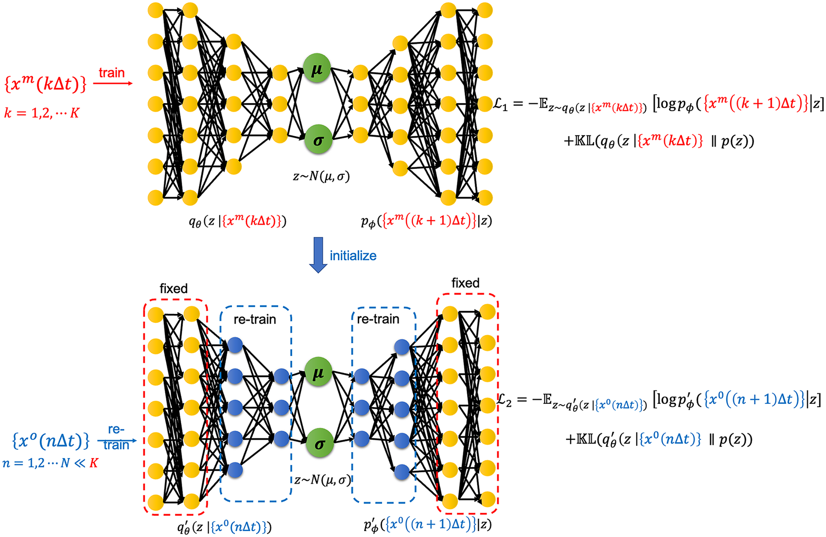
The VAE is trained on nine independent ensembles of the imperfect system with 1,400 consecutive days of climate simulation each with a sampling interval of $ \Delta t $
. Hence, the training size for the VAE is about 12,600 days of data. For transfer learning, we assume that only 10% of the number of training samples is available as noisy observations from the perfect system.
$ \Delta t $
. Hence, the training size for the VAE is about 12,600 days of data. For transfer learning, we assume that only 10% of the number of training samples is available as noisy observations from the perfect system.
3. Results
3.1. Short-term stochastic forecasting on the imperfect system
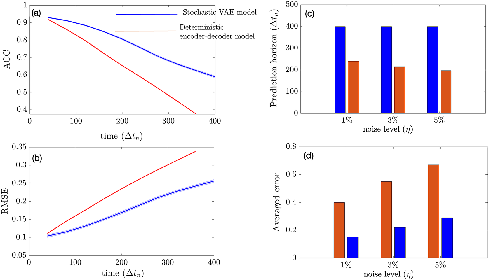
In this section, we show how well the stochastic VAE performs in terms of short-term forecasting on the imperfect system when the initial condition is sampled from the imperfect system. Our baseline model is a convolutional encoder–decoder-based deterministic model that has the exact same architecture as that of the convolutional VAE with the same size of the latent space. During inference, the stochastic VAE generates 100 ensembles at every $ \Delta t $
and the mean of these ensembles is fed back into the VAE autoregressively to predict future time steps. We see from Figure 3 that the stochastic VAE model outperforms the deterministic model. Our experiments suggest that increasing the noise level of the initial condition does not affect the prediction horizon of VAE if we consider ACC
$ \Delta t $
and the mean of these ensembles is fed back into the VAE autoregressively to predict future time steps. We see from Figure 3 that the stochastic VAE model outperforms the deterministic model. Our experiments suggest that increasing the noise level of the initial condition does not affect the prediction horizon of VAE if we consider ACC $ \hskip0.35em =\hskip0.35em 0.60 $
as the limit of prediction (although it is an ad hoc choice) as shown in Figure 3c. This may be attributed to the reduction of initial condition error (due to noise) with ensembling. The averaged RMSE error over 2 days grows faster with an increase in the noise level in the deterministic model as compared to the stochastic VAE model as shown in Figure 3d.
$ \hskip0.35em =\hskip0.35em 0.60 $
as the limit of prediction (although it is an ad hoc choice) as shown in Figure 3c. This may be attributed to the reduction of initial condition error (due to noise) with ensembling. The averaged RMSE error over 2 days grows faster with an increase in the noise level in the deterministic model as compared to the stochastic VAE model as shown in Figure 3d.
Performance of the stochastic convolutional VAE as compared to baseline convolutional encoder–decoder-based model when trained on the imperfect system and predicts from a noisy initial condition sampled from the imperfect system. (a) Anomaly correlation coefficient (ACC) between predicted $ {\psi}_1 $
and true
$ {\psi}_1 $
and true $ {\psi}_1 $
(Murphy and Epstein, Reference Murphy and Epstein1989) from the imperfect system with
$ {\psi}_1 $
(Murphy and Epstein, Reference Murphy and Epstein1989) from the imperfect system with $ \eta \hskip0.35em =\hskip0.35em 5\% $
(noise level) for the initial condition. (b) Same as panel (a), but for RMSE. (c) Prediction horizon (number of
$ \eta \hskip0.35em =\hskip0.35em 5\% $
(noise level) for the initial condition. (b) Same as panel (a), but for RMSE. (c) Prediction horizon (number of $ \Delta {t}_n $
until ACC
$ \Delta {t}_n $
until ACC $ \le \hskip0.35em 0.60 $
) for different noise levels added to the initial condition. (d) Averaged error over 2 days for different noise levels of initial condition. The shading shows the standard deviation across 100 ensembles generated by the VAE model during inference.
$ \le \hskip0.35em 0.60 $
) for different noise levels added to the initial condition. (d) Averaged error over 2 days for different noise levels of initial condition. The shading shows the standard deviation across 100 ensembles generated by the VAE model during inference.
3.2. Short-term stochastic forecasting on the perfect system
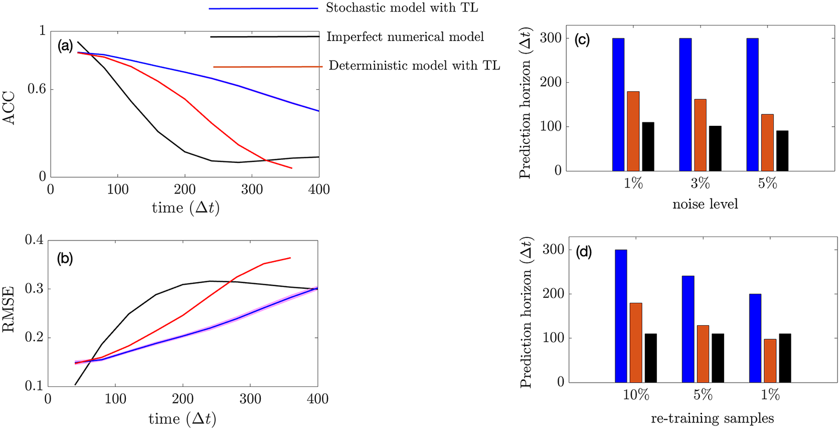
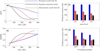
In this section, we show how well the pre-trained VAE (as compared to the baseline encoder–decoder and imperfect numerical model) on the imperfect climate simulations performs on the perfect system when constrained by noisy observations from the perfect system on which it is re-trained. Only two layers before and after the bottleneck layer are re-trained for both the VAE and the baseline model. Figure 4a,b shows that for short-term forecasting, VAE outperforms both the baseline deterministic encoder–decoder model as well as the imperfect numerical model. Figure 4c shows a similar behavior for VAE with an increase in noise level in the initial condition as Figure 3c. Figure 4d shows the effect of the number of re-training samples used as noisy observations for transfer learning on the prediction horizon. While the numerical model is unaffected by the impact of noisy observations (since it does not undergo any learning), an increase in noise level to the initial condition makes it more susceptible to error as compared to the data-driven models which are inherently more robust to noise (due to re-training on noisy observations). In all cases, the VAE outperforms both the deterministic encoder–decoder model and the imperfect numerical model for short-term forecasts.
Performance of the stochastic convolutional VAE compared to that of the baseline convolutional encoder–decoder-based model and the imperfect numerical model when trained on the imperfect system, re-trained on noisy observations from the perfect system, and initialized with a noisy initial condition sampled from the perfect system. (a) Anomaly correlation coefficient (ACC) between predicted $ {\psi}_1 $
and true
$ {\psi}_1 $
and true $ {\psi}_1 $
from the perfect system with
$ {\psi}_1 $
from the perfect system with $ \eta \hskip0.35em =\hskip0.35em 5\% $
(noise level) for the initial condition. (b) Same as panel (a), but for RMSE. (c) Prediction horizon (number of
$ \eta \hskip0.35em =\hskip0.35em 5\% $
(noise level) for the initial condition. (b) Same as panel (a), but for RMSE. (c) Prediction horizon (number of $ \Delta {t}_n $
until ACC
$ \Delta {t}_n $
until ACC $ \le 0.60 $
) for different noise levels added to initial condition. (d) Prediction horizon of the models with different sample sizes of noisy observation data (as percentages of original training sample size) from perfect system. Note that the numerical model is not trained on data and hence would show no effect.
$ \le 0.60 $
) for different noise levels added to initial condition. (d) Prediction horizon of the models with different sample sizes of noisy observation data (as percentages of original training sample size) from perfect system. Note that the numerical model is not trained on data and hence would show no effect.
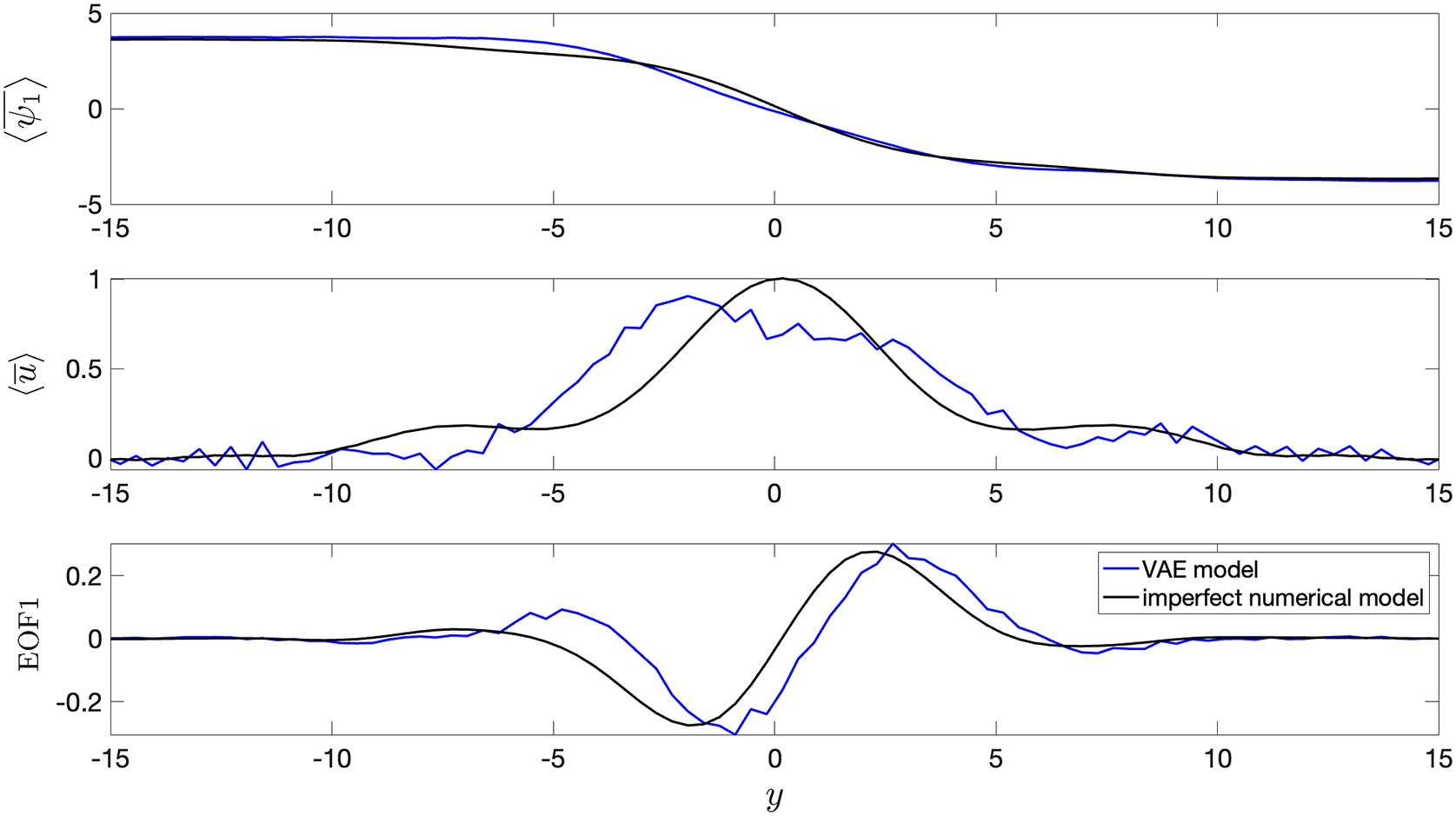
3.3. Long-term climate statistics
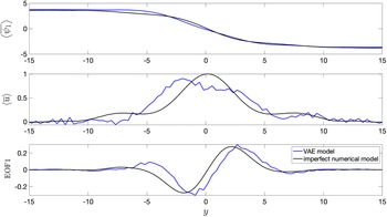
In this section, we show the comparison between long-term climatology obtained from seamlessly integrating the VAE for 20,000 days and the true climatology of the imperfect system. It must be noted that the deterministic encoder–decoder model is not stable and would show unphysical drifts in the climate similar to other deterministic data-driven models within a few days of seamless integration (Chattopadhyay et al., Reference Chattopadhyay, Mustafa, Hassanzadeh and Kashinath2020b). Figure 5 shows stable and non-drifting physical climate obtained from the VAE whose mean of $ {\psi}_j $
,
$ {\psi}_j $
, $ {u}_j $
, and EOF1 of
$ {u}_j $
, and EOF1 of $ {u}_1 $
closely match those of the true system.
$ {u}_1 $
closely match those of the true system.
Long-term climatology obtained from integrating the models for 20,000 days. $ \left\langle {\overline{\psi}}_1\right\rangle $
is the time mean zonally averaged
$ \left\langle {\overline{\psi}}_1\right\rangle $
is the time mean zonally averaged $ {\psi}_1 $
,
$ {\psi}_1 $
, $ \left\langle \overline{u}\right\rangle $
is the time mean zonally averaged upper-layer velocity, and EOF1 is the first EOF (empirical orthogonal function) of
$ \left\langle \overline{u}\right\rangle $
is the time mean zonally averaged upper-layer velocity, and EOF1 is the first EOF (empirical orthogonal function) of $ \left\langle \overline{u}\right\rangle $
. The VAE shows non-drifting physical climate. Baseline encoder–decoder model is not shown since it becomes unstable within 100 days of seamless integration.
$ \left\langle \overline{u}\right\rangle $
. The VAE shows non-drifting physical climate. Baseline encoder–decoder model is not shown since it becomes unstable within 100 days of seamless integration.
4. Conclusion
In this article, we have developed a convolutional VAE for stochastic short-term forecasting and long-term climatology of the stream function of a two-layer QG flow. The VAE is trained on climate simulations from an imperfect QG system before being fine-tuned on noisy observations from a perfect QG system on which it performs both short- and long-term forecasting. The VAE outperforms both the baseline convolutional encoder–decoder model as well as the imperfect numerical model.
One of the main advantages of using the stochastic VAE with multiple ensemble members is the reduction of the effect of noise in the initial condition for short-term forecasting. Moreover, the VAE remains stable through a seamless 20,000 days integration yielding a physical climatology that matches the numerical model. Deterministic data-driven models do not remain stable for long-term integration and hence a stochastic generative modeling approach may be a potential candidate when developing data-driven weather forecasting models that can seamlessly be integrated to yield long-term climate simulations.
Despite the improvement in performance in short-term skills as well as long-term stability, one of the caveats of the VAE is that it is less interpretable as compared to a deterministic model. Moreover, the VAE is more difficult to scale as compared to a deterministic model, especially for high-dimensional systems. This is because one would need to evolve a large number of ensembles for high-dimensional systems, and the exact relationship between short-term skills and long-term stability with the number of ensembles is not well known. Finally, while the application of VAE has resulted in long-term stability, the underlying causal mechanism by which instability is exhibited in a deterministic data-driven model is still largely unknown. Future work needs to be undertaken to understand the cause of this instability such that deterministic models that may be more scalable than VAE can also be used for data-driven weather and climate prediction.
Acknowledgments
This work was started as an internship project by A.C. at Lawrence Berkeley National Laboratory in the summer of 2021 under J.P. and W.B. It was then continued under P.H. as a part of A.C.’s PhD at Rice University. This research used resources of NERSC, a U.S. Department of Energy Office of Science User Facility operated under Contract No. DE-AC02-05CH11231. A.C., E.N., and P.H. were supported by ONR grant N00014-20-1-2722, NASA grant 80NSSC17K0266, and NSF CSSI grant OAC-2005123. A.C. also thanks the Rice University Ken Kennedy Institute for a BP HPC Graduate Fellowship. We are grateful to Kamyar Azizzadenesheli, Mustafa Mustafa, and Sanjeev Raja for providing invaluable advice for this work.
Author Contributions
Conceptualization: A.C., P.H.; Data curation: A.C., E.N.; Formal analysis: A.C.; Funding acquisition: W.B., P.H.; Investigation: A.C., J.P.; Methodology: A.C.; Software: A.C., Supervision: J.P., W.B., P.H.; Validation: A.C.; Visualization: A.C., Writing—original draft: A.C.; Writing—review and editing: A.C., E.N., P.H.
Competing Interests
The authors declare no competing interests exist.
Data Availability Statement
The codes for this work would be available to the public upon publication in this GitHub link: https://github.com/ashesh6810/Stochastic-VAE-for-Digital-Twins.git.
Ethics Statement
The research meets all ethical guidelines, including adherence to the legal requirements of the study country.
Funding Statement
This work received no specific grant from any funding agency, commercial or not-for-profit sectors.
Provenance
This article is part of the Climate Informatics 2022 proceedings and was accepted in Environmental Data Science on the basis of the Climate Informatics peer review process.


 Open access