


1. Introduction
The interactions between liquid drops and fibres is ubiquitous in a wide range of situations including liquid aerosol filtering (Agranovski & Braddock Reference Agranovski and Braddock1998; Zhang et al. Reference Zhang, Liu, Williams, Qu, Feng and Chen2015), coating processes (Quéré Reference Quéré1999; Chan et al. Reference Chan, Lee, Pedersen, Dalnoki-Veress and Carlson2021), digital microfluidics (Gilet, Terwagne & Vandewalle Reference Gilet, Terwagne and Vandewalle2009, Reference Gilet, Terwagne and Vandewalle2010) and fog harvesting (Klemm Reference Klemm2012; Labbé & Duprat Reference Labbé and Duprat2019). The latter has also motivated research of droplets interacting with biological systems (Malik et al. Reference Malik, Clement, Gethin, Krawszik and Parker2014) such as threads of spider silk (Zheng et al. Reference Zheng, Bai, Huang, Tian, Nie, Zhao, Zhai and Jiang2010; Ju, Zheng & Jiang Reference Ju, Zheng and Jiang2014) and plants with fibre-like features such as sequoia needles, cactus spines, grass blades and moss leaves (Limm et al. Reference Limm, Simonin, Bothman and Dawson2009; Ju et al. Reference Ju, Bai, Zheng, Zhao, Fang and Jiang2012; Roth-Nebelsick et al. Reference Roth-Nebelsick, Ebner, Miranda, Gottschalk, Voigt, Gorb, Stegmaier, Sarsour, Linke and Konrad2012; Pan et al. Reference Pan, Pitt, Zhang, Wu, Tao and Truscott2016) that are able to efficiently capture and transport water droplets. In most of these examples, the fibre is generally not still but subject to motion due to external forcing such as wind.
Drops can spontaneously move on horizontal fibres due to spatial gradients in various properties: thickness, most notably with conical fibres (Lorenceau & Quéré Reference Lorenceau and Quéré2004; McCarthy, Vella & Castrejón-Pita Reference McCarthy, Vella and Castrejón-Pita2019; Chan, Yang & Carlson Reference Chan, Yang and Carlson2020), wetting (Zheng et al. Reference Zheng, Bai, Huang, Tian, Nie, Zhao, Zhai and Jiang2010; Ju et al. Reference Ju, Zheng and Jiang2014), temperature (Yarin, Liu & Reneker Reference Yarin, Liu and Reneker2002) or elasticity (Duprat et al. Reference Duprat, Protiere, Beebe and Stone2012). Droplets on non-horizontal fibres slide when the gravitational force overcomes contact angle hysteresis. Gilet et al. (Reference Gilet, Terwagne and Vandewalle2010) studied this in detail for droplets that perfectly wet fibres while Christianto et al. (Reference Christianto, Rahmawan, Semprebon and Kusumaatmaja2022) recently investigated numerically the effect of a finite contact angle. In addition to these passive mechanisms, external perturbations in the form of standing waves (Bick et al. Reference Bick, Boulogne, Sauret and Stone2015) or wind (Dawar et al. Reference Dawar, Li, Dobson and Chase2006; Dawar & Chase Reference Dawar and Chase2008; Sahu et al. Reference Sahu, Sinha-Ray, Yarin and Pourdeyhimi2013; Bintein et al. Reference Bintein, Bense, Clanet and Quéré2019) also lead to directional transport. There have been anecdotal reports pointing to vibrations triggering droplet motion on fibres (Dawar et al. Reference Dawar, Li, Dobson and Chase2006; Dawar & Chase Reference Dawar and Chase2008; Zhang, Lin & Yin Reference Zhang, Lin and Yin2018), yet quantitative data to describe this effect are lacking.
One way to induce reproducible vibrations of droplets is by inducing rigid-body oscillations of the substrate. So far, studies of this phenomenon have only focused on flat, planar surfaces, where two types of experimental set-ups have been employed: droplets on a slanted flat substrate submitted to vertical oscillations, and droplets on a horizontal flat substrate submitted to slanted oscillations. In both cases a directional motion of the droplet is generated for high enough amplitude of oscillations. Recent reviews of experimental, theoretical and numerical results regarding the rich dynamics of these systems are given by Bradshaw & Billingham (Reference Bradshaw and Billingham2018), Deegan (Reference Deegan2020) and Costalonga & Brunet (Reference Costalonga and Brunet2020). In short, a droplet in such a situation experiences a modulation of its contact area through pumping modes of vibrations that periodically stretch and flatten it, while also experiencing rocking lateral vibrations. A schematic illustration of the first pumping and rocking modes is shown in figure 1(a,b). They correspond to the first mode with only radial deformations and to the first mode with azimuthal deformations. Bostwick & Steen (Reference Bostwick and Steen2014) rationalized their existence by adapting the Rayleigh–Lamb theory of vibrating free drops (Rayleigh Reference Rayleigh1879; Lamb Reference Lamb1924) to sessile drops. The combination of both rocking and pumping responses, and in particular their phase difference (Noblin, Kofman & Celestini Reference Noblin, Kofman and Celestini2009), can trigger directional motion. On slanted substrates, a pumping mode alone can trigger motion if the periodic evolution of the wetted area unpins the droplet.

Figure 1. (a,b) Schematic illustration of (a) the first pumping mode and (b) the first rocking mode of a sessile droplet with a mobile contact line on a flat substrate. A pumping droplet flattens and stretches perpendicularly with respect to the substrate, while a rocking droplet vibrates left and right along the substrate. (c) Schematic of the experimental set-up. A well-taut nylon fibre of diameter  $b$ is attached to a structure oscillating vertically with amplitude $A$ and angular frequency $\omega =2{\rm \pi} f$. The fibre makes an angle $\alpha$ with respect to the horizontal direction. As it oscillates and its position evolves as $y_{fibre}=A\cos (\alpha )\cos (\omega t)$, a water droplet of volume $V$ slides down at speed
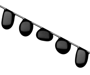
  $\langle U \rangle$. (d) Image a of droplet ( $V=4\ \mathrm {\mu }$l) on a still horizontal fibre ( $\alpha =0^\circ$). The static contact angle between the droplet and nylon fibres is measured to be $\theta =65^\circ \pm 7^\circ$. (e) Images of a droplet over one period $T=1/f$. Here, $V=4\ \mathrm {\mu }$l, $b=200\ \mathrm {\mu }$m, $\alpha =27.5^\circ$, $A=0.10$ mm and $f=60$ Hz. The resulting acceleration from the oscillations is $A\omega ^2=14.2\ {\rm m}\ {\rm s}^{-2}$ so that $\varGamma =A\omega ^2/g=1.45$. The dotted line represents the mean value of $y_{fibre}$ and highlights the fibre's motion. The position of the centre of mass of the droplet projected on the fibre is $x_{drop}$, that of the advancing contact line is $x_a$ and that of the receding contact line is $x_r$. (f) Top image shows the time evolution of the position of a droplet with the same conditions as in (e). The droplet moves at near-constant speed $\langle U \rangle =\langle {\rm d}\kern0.06em x_{drop}/{\rm d}t \rangle = 22.6\ {\rm mm}\ {\rm s}^{-1}$. The bottom image shows the corresponding time evolution of the position of the fibre $y_{fibre}$ (solid line) and of the basal diameter $d=x_a-x_r$ (dashed line).
Quantitatively, for a given frequency of vibrations  $f$, the mechanical amplitude of vibrations $A$ needs to be larger than a threshold $A_{th}$ to trigger motion: for $A>A_{th}$, droplets have a non-zero mean velocity $\langle U \rangle$, defined as the velocity of the centre of mass along the substrate averaged over one period of oscillations; $\langle U \rangle$ is typically in the direction of the oscillations or that of gravity, leading to a sliding droplet with $\langle U \rangle >0$. A less intuitive regime of climbing droplets with $\langle U \rangle <0$ also exists (Brunet, Eggers & Deegan Reference Brunet, Eggers and Deegan2007; Sartori et al. Reference Sartori, Guglielmin, Ferraro, Filippi, Zaltron, Pierno and Mistura2019; Costalonga & Brunet Reference Costalonga and Brunet2020). In the most common case of sliding drops, Costalonga & Brunet (Reference Costalonga and Brunet2020) proposed the following empirical relationship to fit experimental and numerical data:
 \begin{equation} \langle U \rangle-U_0 = s (A-A_{th})^\chi, \quad A>A_{th}. \end{equation}
We have modified this relation to account for  $U_0$, the speed that the droplet has without oscillations. The exponent $\chi$ and the mobility coefficient $s$ quantify the nature of the relationship between the speed and the amplitude. Their values, along with that of $A_{th}$, characterize the response of a droplet on a substrate submitted to oscillations. These parameters depend on the liquid properties (surface tension coefficient, density, viscosity), the size of the droplet, the wetting properties of the substrate, the frequency $f$ of the oscillations and the angles of both the substrate and oscillations with respect to the horizontal direction. Numerical and theoretical works are mostly consistent with $\chi =2$. In particular, Bradshaw & Billingham (Reference Bradshaw and Billingham2018) derived and verified numerically $\langle U \rangle \sim A^2$ for inviscid two-dimensional drops with no contact angle hysteresis and small amplitude of oscillations. Their results also confirm theoretically the importance of the phase shift between the rocking and pumping modes. Experimental investigations on the other hand usually suggest $\chi \simeq 1$, giving a linear relationship between the forcing amplitude and the speed. Yet values of $\chi$ larger than 1 can be also be observed experimentally, and a regime of decreasing speed upon increase of forcing has also been reported by Sartori et al. (Reference Sartori, Guglielmin, Ferraro, Filippi, Zaltron, Pierno and Mistura2019). Overall, the dependence of the coefficients involved in (1.1) is not well understood, even though the experiments by Costalonga & Brunet (Reference Costalonga and Brunet2020) shed some light on the influence of many of the parameters involved for horizontal flat surfaces with low contact angle hysteresis, namely the frequency, viscosity, droplet volume and angle of vibrations. To the best of our knowledge, the effect of the surface geometry has not been explored.
In this article we experimentally probe the behaviour of a droplet placed on a fibre that oscillates vertically. We report the sliding speed as a function of the amplitude and frequency of the forcing. Further, we describe transitions between different regimes in the phase space of the sliding droplet dynamics, which contrasts with prior observations on flat substrates.
2. Experimental set-up
Our experimental set-up is sketched in figure 1(c). A nylon fibre (fishing line, Abu Garcia abulon top) of diameter  $b$ and making an angle $\alpha$ with the horizontal is connected to a mechanical vibrator (PASCO SF-9324). A periodic sinusoidal signal is generated (NI myDAQ), amplified (QSC RMX850a) and fed into the vibrator so that the fibre displacement is $y_{fibre}(t)=A\cos (\alpha )\cos (\omega t)$, where $A$ is the amplitude of the mechanical oscillations and $\omega =2{\rm \pi} f$ their angular frequency. The fibre is taut enough so that it follows a rigid-body motion, and we verified that the precise value of the tension did not influence our results. The tension in the fibre is regularly readjusted to counteract the relaxation of the nylon. The maximum acceleration of the structure resulting from these oscillations is $A\omega ^2$, we normalize it using the gravitational acceleration $g=9.81\ {\rm m}\ {\rm s}^{-2}$ and define the ratio of accelerations as $\varGamma =A\omega ^2/g$. We deposit a droplet of volume $V$, equivalent spherical radius $r=(3V/4{\rm \pi} )^{1/3}$, onto the oscillating fibre with a micropipette and record its motion over approximately 40 mm along the fibre as it slides downward. The droplet motion is recorded with a high speed camera (Photron FASTCAM Mini) with a frame rate ranging from a few hundreds and up to 5000 f.p.s.; the typical resolution is $20\ \mathrm {\mu }{\rm m}\ {\rm pixel}^{-1}$ using a standard macro lens. Droplets are made of deionized water with a small amount of black die (nigrosin) to facilitate visualization. The relevant physical properties of water are its density $\rho =1.0 \times 10^3\ {\rm kg}\ {\rm m}^{-3}$, surface tension coefficient $\sigma =70\ {\rm mN}\ {\rm m}^{-1}$ and dynamic viscosity $\mu =1\ {\rm mPa}\ {\cdot}\ {\rm s}$. Experiments are performed at ambient temperature (22 $^\circ$C) and the droplet's evaporation is negligible over the time scale associated with its motion. Representative images and measurements are shown in figure 1(e,f). Between each experiment the fibre is cleaned with lint-free wipes soaked in acetone and a new droplet is placed on the fibre once the acetone has fully evaporated.
Inferring the contact angle of a droplet on a fibre is not straightforward (figure 1d). To measure the contact angle between nylon and water we used the following procedure. A glass slide is cleaned with isopropanol before being placed on top of small pieces of nylon fibre. This set-up is placed in an oven with a temperature just above the melting point of nylon. Once the nylon-covered glass slide is cooled to room temperature, the nylon film is peeled away and gives a uniform and flat film. We deposited 2  $\mathrm {\mu }$l water droplets on this nylon film and measured the contact angle using a subpixel edge detection method (Trujillo-Pino et al. Reference Trujillo-Pino, Krissian, Alemán-Flores and Santana-Cedrés2013). The static contact angle is $\theta =65^\circ \pm 7^\circ$, close to previously reported contact angle values for water droplets on nylon.
The behaviour of droplets on oscillating substrates depends strongly on the frequency  $f$ of the forcing oscillations, and in particular on the ratio $f/f_{pump}$, with $f_{pump}$ the natural frequency of the first pumping mode of the droplet (Costalonga & Brunet Reference Costalonga and Brunet2020). The natural frequencies of vibrations of inviscid droplets scale as $(\sigma /\rho V)^{1/2}$ and the full analytical expression for freely suspended spherical drops is well known (Rayleigh Reference Rayleigh1879; Lamb Reference Lamb1924). Sessile droplets on flat and horizontal surfaces exhibit different responses due to the change of geometry: this has been studied in detail by Bostwick & Steen (Reference Bostwick and Steen2014) and Chang et al. (Reference Chang, Bostwick, Daniel and Steen2015). We also expect drops on fibres to exhibit different eigenmodes and natural frequencies that are a function of the fibre diameter $b$ and of the wetting properties of the substrate. Here, we measure the first natural frequency $f_{pump}$ of pumping oscillations by subjecting a droplet with $V=4\ \mathrm {\mu }$l ( $r\simeq 1$ mm) deposited on a horizontal fibre ( $\alpha =0^\circ$) with diameter $b=200\ \mathrm {\mu }$m to a step vertical acceleration. We recorded the distance between the bottom of the fibre and the tip of the droplet following this impulse: this generates a periodic decaying signal with frequency $f_{pump}=57 \pm 1$ Hz.
To quantify the expected effect of viscosity in the droplet's behaviour, an important parameter is the ratio between the thickness of the Stokes’ boundary layer  $\delta =(2\mu /\rho \omega )^{1/2}$ and the characteristic size of the droplet, taken here as its equivalent spherical radius $r=(3V/4{\rm \pi} )^{1/3}$. Even for the smallest frequency we have used, the Stokes layer is much thinner than the droplet itself: $\delta \approx 0.15~{\rm mm} \ll r \approx 1$ mm for a $V=4\ \mathrm {\mu }$l water droplet on a fibre oscillating at $f=15$ Hz. This is equivalent to a large Reynolds number $Re =\rho (r\omega )r/\mu =2(r/\delta )^2\gtrsim 100$. This suggests that viscous effects are localized in a thin boundary layer and that the flow in most of the droplet is inertial. Another measure of the importance of viscosity is the Ohnesorge number $Oh =\mu (\rho r \sigma )^{-1/2}$, the inverse squared Reynolds number based on the capillary speed $\sigma /\mu$, which compares viscous effects with both inertial and capillary ones; here, $Oh \approx 4\times 10^{-3} \ll 1$. The Weber number comparing inertial with capillary effects is $We =\rho (r\omega )^2r/\sigma$ and ranges from $0.1$ to $10$ upon varying the frequency from 15 to 135 Hz, suggesting a competition between inertia and capillarity. We consider droplets that are larger than the fibre they are deposited on, $r>b$, but smaller than the capillary length $l_c=(\sigma /\rho g)^{1/2} \approx 3$ mm so that the Bond number quantifying the ratio of capillary to gravitational effects is $Bo =(r/l_c)^2 \approx 0.1$. While smaller than 1, this Bond number is large enough for gravity to significantly modify the equilibrium shape (Gupta et al. Reference Gupta, Konicek, King, Iqtidar, Yeganeh and Stone2021) and the droplets we study sag on the fibre, see figure 1(d,e).
3. Droplet sliding speed
Our main dataset focuses on a nylon fibre of diameter  $b=200\ \mathrm {\mu }$m making an angle $\alpha =27.5^\circ$ with the horizontal, on which a water droplet of volume $V=4\ \mathrm {\mu }$l is deposited. We systematically vary the frequency of oscillations from $f=15$ to 135 Hz, and the amplitude from zero and up to the detachment of the droplet from the fibre. Reported values of the speed of the droplet $\langle U \rangle$ shown throughout the article (figures 2, 9, 10 and 11) represent the mean and standard deviation of typically 3 different experiments. We note that, with these parameters, the droplet naturally slides down the fibre with a speed $U_0=2.5 \pm 1.6\ {\rm m}\ {\rm s}^{-1}$, the droplet's speed without vibrations ( $A=0,\varGamma =0$). We believe that this large relative error originates from small defects and chemical inhomogeneities in the nylon fishing lines, which can affect the contact angle dynamics. We will also show that there is no significant qualitative change in our observations when the droplet is pinned to the fibre ( $U_0=0$) for lower angles $\alpha$ or large diameters $b$.
$b$.

Figure 2. Experimental results regarding the droplet's sliding speed  $\langle U \rangle$ with $V=4\ \mathrm {\mu }$l, $b=200\ \mathrm {\mu }$m, $\alpha =27.5^\circ$. (a) Mobility parameter $s={\rm d}\langle U \rangle /{\rm d}A$ obtained from a linear fit as a function of the forcing frequency $f$ considering only droplets responding with a harmonic pumping mode. Panels (b–e) show $\langle U \rangle$ as a function of the normalized forcing acceleration $\varGamma$ for various frequencies $f$. Filled symbols represent experiments where the droplet exhibits harmonic pumping vibrations. Open symbols represent experiments where the droplet: (c) exhibits subharmonic pumping vibrations at frequency $f/2$; (d) exhibits both harmonic pumping and rocking modes; (e) swings subharmonically in a pendulum-like fashion at $f/2$. These various responses are illustrated in figures 4, 5 and 6, respectively. We have chosen to represent $\langle U \rangle$ as a function of the normalized acceleration $\varGamma =A\omega ^2/g$ rather than as a function of the amplitude $A$: this allows us to more easily compare data with different frequencies. The resonant response shown in (a) is also evident when representing the averaged slope ${\rm d}\langle U \rangle /{\rm d}\gamma$ as a function of $f$ (not shown).
As we discussed in the Introduction, § 1, an empirical correlation between the forcing amplitude and the droplet's speed is given by (1.1), which is typically linear ( $\chi =1$) in most experimental work using flat substrates. We therefore expect a linear relationship between the droplet sliding speed and the amplitude of vibrations as $\langle U \rangle -U_0 = s(A-A_{th})$ for $A>A_{th}$, which allows us to define a constant $s={\rm d}\langle U \rangle /{\rm d}A$. In figure 2(a) we show the evolution of $s$ as a function of the forcing frequency $f$: we observe a resonant behaviour with a maximum for $f \approx 50$ Hz, which is near but slightly below the natural pumping frequency $f_{pump}=57$ Hz discussed in § 2. We note that Costalonga & Brunet (Reference Costalonga and Brunet2020), using a different set-up, found a maximum of mobility $s$ for a frequency close to, but in their case larger than, $f_{pump}$. Figure 2(b) shows $\langle U \rangle$ as a function of $\varGamma$ for selected frequencies where the linear relation (1.1) with $\chi =1$ indeed seems to be satisfactory.
In figure 2(a) we extract  $s$ only considering droplets that respond solely with harmonic pumping. This mode of response is shown in figure 1(e) and is the analogue of the pumping response for a flat substrate (figure 1a): the droplet periodically stretches and flattens perpendicularly to the fibre, and with the same frequency as the forcing frequency $f$. The associated data are represented with filled markers in figure 2(b–e); we will discuss in the next section the other regimes we have observed. When the relationship between the droplet's speed and the forcing amplitude is nonlinear, we extracted $s$ from a linear fit but for small amplitudes only in order to compare with the other datasets. Indeed, while the exponent $\chi =1$ is reasonable for most frequencies, some of the data would be fitted more adequately with $\chi > 1$, e.g. $f=15$ Hz in figure 2(b). Such superlinear behaviour is common in numerical studies and has also been observed in some of the experiments of Costalonga & Brunet (Reference Costalonga and Brunet2020). In Appendix A we show data with a smaller tilt angle $\alpha =15$ and $7.5^\circ$ (figure 9) and with larger fibre diameters $b=400$ and 600 $\mathrm {\mu }$m (figure 10): in these cases $U_0=0$, and we still observe a monotonic increase of the sliding speed as a function of the amplitude of vibrations for harmonically pumping droplets. Varying the tilt angle still yields $\chi \approx 1$, while increasing the fibre diameter gives more consistently a sublinear behaviour with $\chi <1$.
Harmonic pumping vibrations of the droplet modulate its basal diameter  $d$ at the forcing frequency $f$. To investigate the relationship between the droplet's speed and the amplitude of oscillations, we first consider the average diameter $\langle d \rangle =(1/T)\int _0^T \, {\rm d}(t)\,{\rm d}t$. Figure 3(a) shows a correlation between $\langle d \rangle$ and the average droplet sliding speed $\langle U \rangle$, with a collapse of the data obtained at different frequencies: as the amplitude of fibre's oscillations increases, $\langle d \rangle$ decreases while $\langle U \rangle$ increases. We note that, given the shape of the droplet, $d$ is proportional to the wetted area of the droplet on the fibre $S\simeq {\rm \pi}b d$. It is, however, unclear how we should understand this link. There are three forces acting on the droplet along the fibre: the gravitational force $F_g=\rho g V \sin (\alpha )$, the viscous frictional force $F_v \sim d \mu U$ and the capillary force $F_c \sim \sigma b$. The viscous force depends on the distribution of shear stress: this has not been studied for non-axisymmetric droplets with a finite contact angle on fibres, even in the case of steady sliding, except for axisymmetric and perfectly wetting drops (Lorenceau & Quéré Reference Lorenceau and Quéré2004; Gilet et al. Reference Gilet, Terwagne and Vandewalle2010). The capillary force is the unbalanced Young's force which depends on the dynamic apparent contact angles, it is not possible to accurately estimate this in our experimental set-up. Additional experiments (see Appendix A) suggest that the driving force leading to sliding is gravity and that it is mostly resisted by the unbalanced Young's force, not by viscous drag. We therefore believe that the link between sliding speed and averaged basal diameter (figure 3a) reflects indirectly a dependence on the distribution of dynamic contact angles around the fibre.

Figure 3. Data corresponding to  $V=4\ \mathrm {\mu }$l, $b=200\ \mathrm {\mu }$m, $\alpha =27.5^\circ$. (a) Droplet's sliding speed $\langle U \rangle$ as a function of the averaged basal diameter $\langle d \rangle =\int _0^T \,{\rm d}(t)\,{\rm d}t/T$ for various frequencies $f$ upon varying the amplitude of the oscillations. Filled symbols represent data where the droplet exhibits a harmonic pumping mode. Open circles ( $\circ$) for $f=90$ Hz correspond to subharmonic pumping while open upwards triangle ( $\triangle$) for $f=120$ Hz correspond to a combination of pumping and rocking modes. (b) Phase angle $\beta$ between the basal diameter $d$ and the fibre's position $y_{fibre}$ as a function of the amplitude of oscillations for three representative frequencies. Only droplets showing a harmonic pumping mode are considered. (c) Mean value of $\beta$ averaged over all amplitudes as a function of the frequency $f$. To account for the fact that an angle is defined modulo $2{\rm \pi}$, the mean value and standard deviation used as error bars in (b) and (c) are defined as the following directional moments: $\arg (m)$ and $(-2\ln (\lvert m\rvert ))^{1/2}$, respectively, with $m=\sum _{j=1}^n \exp ({\rm i}\beta _j)/n$.
It is also interesting to look at the phase angle  $\beta$ between the basal diameter $d$ and the fibre position $y_{fibre}$: $\beta =0$ or $2{\rm \pi}$ corresponds to an evolution where $d$ is maximal at the crest of the fibre's oscillations, while $\beta ={\rm \pi}$ corresponds to the opposite situation where $d$ is minimal at the crest. Figure 1(e,f) shows an example where $\beta \approx {\rm \pi}$. We systematically extracted $\beta$ using a Fourier analysis of the two signals $d(t)$ and $y_{fibre}(t)$. Figure 3(b) shows the evolution of $\beta$ with the acceleration $\varGamma$ for three representative frequencies, while figure 3(c) shows $\beta$, averaged over all $\varGamma$, as a function of the frequency. For a fixed frequency there is generally little change of $\beta$ upon varying the acceleration: for $f\lesssim 40$ Hz, $\beta \gtrsim 3{\rm \pi} /2$, while it drops to $\beta \approx {\rm \pi}$ for $f\gtrsim 50$ Hz. For $f=45,47.5$ and 50 Hz, near the resonance peak shown in figure 2(a), $\beta$ continuously decreases with $\varGamma$. We note that $\beta$ has been correlated with the speed and mobility of droplets in prior works on vibrating flat substrate. Sartori et al. (Reference Sartori, Guglielmin, Ferraro, Filippi, Zaltron, Pierno and Mistura2019) delimited regimes of descending and fast descending droplets, where $\beta \approx {\rm \pi}$ in the descending regime and $\beta$ close to 0, or $2{\rm \pi}$, in the fast descending regime. Similarly Costalonga & Brunet (Reference Costalonga and Brunet2020) found $\beta \approx 0$ near the maximum droplet mobility $s$, while $\beta \approx {\rm \pi}$ corresponds to climbing drops in their experiments.
The discussion above only focused on droplets responding to the fibre's oscillations with a harmonic pumping motion, but this is not the only interfacial motion that is generated. While figures 1(e,f) and 2(a,b) summarize some of our observations on the droplet speed as a function of the amplitude, it also hides some complex interfacial flows: we have observed different regimes of droplet response for  $f\approx 90$ Hz, $f\geq 120$ Hz and $30 \lesssim f\lesssim 45$ Hz. We show in figure 2(c–e) the effects that these different regimes have on the sliding speed and focus next on these.
4. Regimes of droplet response
For some forcing frequencies the droplet can transition from one regime of vibrations to another upon increasing the forcing amplitude, with important effects on the sliding speed. We now discuss these different transitions in turn.
4.1. Transition from harmonic to subharmonic pumping for  $f \approx 90\ {\rm Hz}$

Figure 2(c) shows  $\langle U \rangle$ as a function of $\varGamma$ for $f=90$ and 95 Hz. Above a threshold normalized acceleration $\varGamma _{sub} \simeq 5$ and $6$, respectively, we observe that the droplet transitions from a regime of harmonic pumping to a regime of subharmonic pumping, where the droplet responds at half the forcing frequency $f$. We also observed the same behaviour for $f=85$ Hz, not shown for clarity since the corresponding data are very close to those with $f=90$ Hz. This transition from harmonic to subharmonic response corresponds to a sharp increase of the sliding speed $\langle U \rangle$ for $f=85$ and 90 Hz. There is also an increase, albeit more moderate, at $f=95$ Hz.
Figure 4 shows the difference in the shapes and dynamics of two representative experiments performed at  $f=90$ Hz and near $\varGamma _{sub}$, with a harmonic response for $\varGamma =4.7<\varGamma _{sub}$ and a subharmonic response for $\varGamma =5.5>\varGamma _{sub}$. Despite a relatively small change in the forcing amplitude, we observe a doubling of the speed of the droplet's centre of mass $\langle U \rangle$. Interestingly, one of the most obvious differences between the two droplets is regarding their basal diameter $d$. It shows little variation in the harmonic regime, evolving from 1.4 to 1.8 mm, compared with the subharmonic region, when it goes down to 1 and up to 2 mm. Its averaged value $\langle d \rangle$ is also smaller in the subharmonic case, and in fact figure 3(a) shows that the correlation between $\langle d \rangle$ and $\langle U \rangle$ previously discussed still holds. In Appendix A we show that this subharmonic response appears and also causes a jump in speed for thicker fibres or smaller tilt angles.

Figure 4. Illustration of the harmonic and subharmonic droplet behaviours observed at  $f=90$ Hz with $V=4\ \mathrm {\mu }$l, $b=200\ \mathrm {\mu }$m, $\alpha =27.5^\circ$ and (a,b) $A=0.14$ mm, $\varGamma =4.7$ (c,d) $A=0.17$ mm, $\varGamma =5.5$. (a,c) Snapshots showing that the shape of the droplet is periodic with period $T$ and $2T$, respectively. The dotted line is fixed in the laboratory frame and represents the maximum position of the fibre, which highlights its oscillations. (b,d) Corresponding evolution of the fibre's position (solid line) and basal diameter (dashed line). The mean value of the droplet's speed is (a,b) $\langle U \rangle =31\ {\rm mm}\ {\rm s}^{-1}$ and (c,d) $\langle U \rangle =58\ {\rm mm}\ {\rm s}^{-1}$. See supplementary movies 1 and 2 available at https://doi.org/10.1017/jfm.2023.462.
It is interesting to put these observations into perspective with prior work on droplets moving on a flat substrate. First, the existence of a subharmonic behaviour above a forcing threshold is reminiscent of the parametric Faraday instability (Miles & Henderson Reference Miles and Henderson1990) and is the result of a competition between inertia and capillarity. Subharmonic droplet deformations are commonly observed on forced sessile droplets on flat substrates (Chang et al. Reference Chang, Bostwick, Daniel and Steen2015; Chang, Daniel & Steen Reference Chang, Daniel and Steen2017). Maksymov & Pototsky (Reference Maksymov and Pototsky2019) showed, using an inertial thin film model, that, for small forcing accelerations, droplets respond harmonically, and that subharmonic Faraday waves only occur above a threshold acceleration. Costalonga & Brunet (Reference Costalonga and Brunet2020) observed experimentally the possibility of subharmonic response in their set-up of droplets on a horizontal substrate submitted to slanted vibrations. However, they report a transition from harmonic response for sliding droplets ( $\langle U \rangle >0$) to subharmonic response for climbing droplets ( $\langle U \rangle <0$), while we observe an acceleration of the descending speed in the subharmonic regime. We also note that they obtained a subharmonic regime for $f\simeq 1.5f_{pump}$; this 1.5 factor also matches our experiments ( $1.5 f_{pump} \simeq 85$ Hz). Second, using droplets on tilted liquid infused substrates submitted to vertical vibrations, Sartori et al. (Reference Sartori, Guglielmin, Ferraro, Filippi, Zaltron, Pierno and Mistura2019) observed experimentally above a threshold acceleration a regime that they refer to as fast descending, where droplets slide much faster. This regime is associated with a basal diameter showing much more important variations than in the regular descending regime, similarly to our experiments. Finally, through numerical simulations, Ding et al. (Reference Ding, Zhu, Gao and Lu2018) reproduced the experiments of Brunet et al. (Reference Brunet, Eggers and Deegan2007) of droplets on tilted substrates with vertical vibrations. Their results suggest the strong importance of a non-sinusoidal evolution of the wetted area $S\approx {\rm \pi}b d$. We also see in figure 4(b,d) that $d$ switches from near-sinusoidal in the harmonic case to completely non-sinusoidal when the response is subharmonic.
4.2. Transition from pumping to rocking for $f \geq 120\ {\rm Hz}$

Most droplets we have observed only exhibit a pumping mode, shown already in figures 1(b,c) and 4. For  $f=120$ and 135 Hz and for high enough amplitude of vibrations, we observe a transition where the droplet can exhibit a combination of pumping and rocking modes. This is illustrated in figure 5. The existence of this rocking mode is particularly evident when considering the instantaneous speed ${\rm d}\kern0.06em x_{drop}/{\rm d}t$, figure 5(e). In the pumping-only mode, the droplet exhibits a near-constant velocity, showing variations of $\approx$20 % around the mean value $\langle U \rangle$: this is because pumping vibrations are mostly normal to the fibre. When the rocking mode appears, lateral vibrations become significant and the speed of the centre of mass of the droplet shows significant variations around the mean.

Figure 5. Droplets with  $f=120$ Hz, $V=4\ \mathrm {\mu }$l, $b=200\ \mathrm {\mu }$m, $\alpha =27.5^\circ$ and (a,b) $A=0.23$ mm, $\varGamma =13.4$ (c,d) $A=0.31$ mm, $\varGamma =18.0$. The difference in the shape of the droplet over one period is illustrated in (a,b). The dotted line represents the maximum value of $y_{fibre}$ and highlights the fibre's vibrations. Panels (c) and (d) show the time evolution of the basal diameter for the droplets in (a) and (b), respectively. (e) Instantaneous droplet speed. Averaged over one period, the mean value is (a) $\langle U \rangle =38\ {\rm mm}\ {\rm s}^{-1}$ and (b) $\langle U \rangle =83\ {\rm mm}\ {\rm s}^{-1}$. See supplementary movies 3 and 4 available in the supplementary material.
As shown in figure 2(d), this rocking mode significantly increases the sliding speed  $\langle U \rangle$. This happens despite the fact that the averaged basal diameter $\langle d \rangle$ is larger in the presence of the rocking mode (figure 5c,d), and the correlation of figure 3 does not hold anymore. In this regime the combined effects of rocking and pumping cannot be captured solely by the change in wetted area, similarly to what is observed on droplets on horizontal flat surfaces submitted to slanted vibrations (see Costalonga & Brunet (Reference Costalonga and Brunet2020) and the discussion in § 1).
4.3. Transition between pumping and swinging for $30\ {\rm Hz} \lesssim f \lesssim 45\ {\rm Hz}$

Figure 2(e) shows the speed of droplets as a function of the amplitude of oscillations for  $f=30,40$ and 45 Hz. For these three frequencies the droplet can respond by swinging across the fibre similarly to a pendulum, as illustrated in figure 6. This swinging motion is subharmonic at half the forcing frequency.

Figure 6. Droplets at  $f=30$ Hz $V=4\ \mathrm {\mu }$l, $b=200\ \mathrm {\mu }$m, $\alpha =27.5^\circ$ and $A=0.26$ mm, $\varGamma =0.96$. (a,b) Vibrating-only regime where the droplet slides at $\langle U \rangle =18\ {\rm mm}\ {\rm s}^{-1}$, (c,d) Subharmonic swinging regime where the droplet slides at $\langle U \rangle =31\ {\rm mm}\ {\rm s}^{-1}$. (a,c) View from the side and (b,d) from the top, looking down at the droplet. (e) Time evolution of the basal diameter $d$ extracted from the movies corresponding to (a,b) and (c,d). In the latter case, when the droplet swings, we did not extract $d$ with automatic image processing but did manual measurements combining both the side and top views as needed. We could not extract accurate data for $0< t<0.5T$ and $T< t<1.5T$. See supplementary movies 5–8 available in the supplementary material.
At  $f=30$ Hz, the swinging motion is only observed for high enough amplitude of oscillations and when droplets are significantly perturbed or after being deposited on the fibre (e.g. due to the detachment from the micropipette, or by flicking the oscillating structure). When they are gently deposited on a still fibre with a slowly increasing amplitude of oscillations, only the harmonic pumping response is observed. However, once they enter the swinging mode they do not return to harmonic pumping. Henceforth, for $f=30\ {\rm Hz}$, the harmonic pumping response is unstable to finite perturbations. Figure 2(e) shows that the transition to the swinging mode significantly increases the sliding speed.
Figure 6(e) shows that, in the swinging mode, the basal diameter  $d$ and hence the wetting area $S$ are significantly smaller than in the pumping case. This can be understood at least partly by considering the centrifugal acceleration induced by the swinging motion. The droplet has an equivalent spherical radius $r=(3V/4{\rm \pi} )^{1/3} \simeq 1$ mm and swings at $f/2$ so that its angular velocity can be approximated, on average, as $\omega /2$. The resulting centrifugal acceleration is $r\omega /2 \approx 9\ {\rm m}\ {\rm s}^{-2}$, which is comparable to both the gravitational acceleration and to the acceleration induced by the fibre motion (here $\varGamma \simeq 1$ and hence $A\omega ^2 \simeq g=9.8\ {\rm m}\ {\rm s}^{-2}$). This supports the idea that the centrifugal acceleration due to swinging pushes the droplet away from the fibre, diminishing its wetting area. However, the data would not collapse on figure 3(a) showing the correlation between $\langle d \rangle$ and $\langle U \rangle$; this is not surprising and shows that energy is dissipated differently as the flow inside the droplet is very different when swinging as compared with when it is pumping.
When increasing the frequency to  $f=40$ Hz, harmonic pumping becomes more and more unstable and eventually cannot be reached anymore. Here, we only observe subharmonic swinging even at low amplitude of oscillations. Increasing again the frequency to $f=45$ Hz, we also only observed subharmonic swinging at low amplitude. However, upon increasing the amplitude the droplet switches to a subharmonic pumping mode. At this frequency ( $\,f=45$ Hz) it is now the swinging mode that becomes unstable at high amplitude; this transition also increases drastically the sliding speed (figure 2e). Data with a different fibre diameter and different tilt angles shown in Appendix A also exhibit this behaviour.
While the two previously discussed regimes of rocking and subharmonic pumping are also observed on flat vibrating substrates, swinging droplets can only occur on fibres. Next, we aim to rationalize the existence of this swinging mode.
5. Droplet swinging around a horizontal fibre
5.1. Experiments
In order to obtain a clearer picture of the pendulum-like swinging droplet motion illustrated in figure 6, we focus on droplets on horizontal fibres ( $\alpha =0^\circ$) to decouple the droplet's sliding motion from its response to oscillations. We construct a regime map from experiments, where we observe three different behaviours: harmonic vibrations, subharmonic vibrations and swinging. This is shown in figure 7, confirming the observations in § 3 on tilted fibres, namely, the existence of a subharmonic swinging regime for $f$ ranging from approximately 30 and up to 45 Hz, and a subharmonic vibration starting near $80$ Hz. This regime map is obtained as follow: at a given frequency, the amplitude of oscillations is increased from 0 and up to a change of regime of vibrations or detachment of the droplet from the fibre. Care was taken to ensure that the rate of the amplitude sweep, ${\rm d}A/{\rm d}t$, was small enough to not influence the measured threshold represented as symbols in figure 7. For each threshold, this procedure was repeated five times to obtain standard deviations shown by the error bars. For thresholds corresponding to transitions between two regimes of vibrations, the same procedure was then repeated starting from a high amplitude of oscillations and slowly lowering it. The two procedures, increasing or lowering the amplitude of oscillations, give slightly different thresholds; this explains the overlap between regions of harmonic and subharmonic pumping for $f\geq 80$ Hz. Figure 7 also shows a region where both a harmonic vibrating droplets and subharmonic swinging droplets can coexist. In the latter regime, subharmonic swinging only takes place if a finite perturbation is introduced in the system (e.g. blowing gently on the droplet, depositing the droplet on an already vibrating fibre or flicking the vibrating structure), or when decreasing the amplitude of vibrations from the region where only swinging motion occurs. Once a droplet is in the subharmonic swinging mode it enters a stable state, and we never observed a droplet switching from a swinging to a non-swinging motion. For $f=25$ and $30$ Hz, the structure was flicked manually to see if swinging could take place. At these two frequencies the region of swinging motion is bounded from above below the ejection threshold: this is not because the droplet switches to harmonic vibrations upon increasing the amplitude, but because it detaches from the fibre when the swinging mode is excited at higher amplitudes.

Figure 7. Regime map of the three different droplet behaviours ( $V=4\ \mathrm {\mu }$l) on a horizontal fibre ( $\alpha =0^\circ$) of thickness $b=200\ \mathrm {\mu }$m. The region between the horizontal line $\varGamma =0$ and the circles, in blue, represents the regime of harmonic vibrations. The region between triangles, in green, represents the regime of subharmonic vibrations at $f/2$. The region between squares, in red, represents the regime of subharmonic swinging at $f/2$. The grey hatched region between 45 and 47 Hz corresponds to a narrow range of frequencies where it is challenging to obtain reproducible results. The top axis represents the dimensionless frequency $\omega /\omega _p$, with $f_p=\omega _p/2{\rm \pi}$ the pendulum frequency discussed in the text. We have used $f_p=15$ Hz.
5.2. Analogy with a forced pendulum
The swinging motion of the droplet is reminiscent of a pendulum. We illustrate this analogy in figure 8(a,b) between a droplet hanging below an oscillating fibre and a pendulum with constant length  $L_{eq}$, mass $m$, in the gravitational field $g$ and submitted to vertical oscillations of its support as $A\cos (\omega t)$. By making this analogy we assume the droplet to be a solid with a motion described by a single degree of freedom, the angle $\phi$ with respect to the vertical direction, and ignore any interface deformations. This system obeys the following damped Mathieu equation (Kovacic, Rand & Sah Reference Kovacic, Rand and Sah2018), which is the classical pendulum equation written in the frame of the oscillating support:
 \begin{equation} \phi''(t) + 2{c_p}{\omega_p}\phi'(t)+\omega_p^2(1-\varGamma\cos(\omega t))\phi(t)=0,\quad \omega_p=(g/L_{eq})^{1/2}, \end{equation}
where  $({\cdot })'={\rm d}({\cdot } )/{\rm d}t$ denotes the derivative with respect to time, and $\omega _p$ is the natural frequency of pendulum oscillations. We have assumed small angles with $\vert \phi (t) \vert \ll 1$, and to account for dissipation we have included a linear damping term characterized by the dimensionless friction coefficient $c_p$. Equation (5.1) is an archetype for parametric instabilities with connections to a wide range of physical phenomena and has been studied extensively (Kovacic et al. Reference Kovacic, Rand and Sah2018). The equilibrium position $\phi =0$ is unstable for large enough values of the forcing $\varGamma$ at driving frequencies $\omega \approx 2\omega _p/n$, with $n=1,2,3,\ldots$ a positive integer. The most unstable mode corresponds to $n=1$, $\omega \simeq 2\omega _0$, where the pendulum then swings subharmonically at $\omega /2$. A stability diagram of (5.1) is shown in figure 8(d) where the greyed regions represent the so-called Arnold tongues of instability, where the position $\phi =0$ is linearly unstable and the oscillations of the substrate make the pendulum swings. The Arnold tongues would go down to $\varGamma =0$ in the undamped case ( $c_p=0$), the main effect of damping is to shift the tongue of instabilities to higher values of $\varGamma$.

Figure 8. Analogy between (a) a droplet swinging of a fibre – visualized in a plane perpendicular to the cross-section of the fibre – and (b) a simple pendulum or (c) an elastic pendulum with spring constant  $k$, with a point mass $m$ and an equilibrium length $L_{eq}$. The system is placed in the gravitational field $g$, the support oscillates as $A\cos \omega t$ and $\phi$ denotes the angle with respect to the vertical. (d) Linear stability diagrams of (5.2) for a simple pendulum and an elastic pendulum for different values of $\varOmega =\omega _p/\omega _s$, the ratio of the natural frequency of the pendulum motion $\omega _p=(g/L_{eq})^{1/2}$ to that of the spring motion $\omega _s=(k/m)^{1/2}$. The damping coefficients are $c_s=c_p=0.15$, and $\varGamma =A\omega ^2/g$ is the dimensionless forcing acceleration.
We assume that a droplet sagging on a fibre can be mimicked as a simple pendulum and can then be modelled by (5.1), with  $L_{eq}=I/a$, $\omega _p=(mga/I)^{1/2}$ for a physical pendulum with a homogeneous distribution of mass. Here, $a$ is the distance from the axis of rotation to the centre of mass of the droplet and $I$ the moment of inertia of the droplet about the axis of rotation. We estimate $a$ and $I$ from experimental images of a droplet on a static fibre ( $\varGamma =0$) and find $f_p = \omega _p/2{\rm \pi} \approx 15$ Hz for a $4\ \mathrm {\mu }$l water droplet on a $200\ \mathrm {\mu }$m horizontal nylon fibre. From the discussion above we would then expect to observe a swinging motion centred around $f\approx 2f_p=30$ Hz. Experiments show that the range of unstable frequencies is $30\ {\rm Hz} \lesssim f\lesssim 45\ {\rm Hz}$.
One explanation to this discrepancy could be an inaccurate estimation of the natural frequency  $f_p$. Another experimental procedure to measure it, distinct from the geometrical method described above, is to induce the swinging motion of the droplet on a still fibre and directly observe the period of oscillations. When perturbing the droplet using a mechanical impulse or blowing on it on a still fibre we, however, did not manage to induce significant oscillations without detaching the droplet. Instead, we oscillated the fibre for the droplet to naturally swing, and suddenly stopped the oscillations. The measured oscillation frequency is in this case $21$ Hz, which is different than the previous estimate $f_p=15$ Hz. This would predict a swinging motion with a tongue of instability centred around $21$ Hz, which might be considered to be in better agreement with our experimental results but still does not capture some of the experimental features, and in particular the fact that swinging cannot be observed above 45 Hz. With this method, however, the droplet is both swinging and vibrating in a pumping mode, and we cannot exclude an effect of the vibrations on the swinging itself. This is in fact always true and hints at the fact that the droplet pumping mode of response should be considered to explain the swinging region in the phase diagram shown in figure 7.
5.3. Analogy with a forced elastic pendulum
To account for the vibrations of the droplet itself, in addition to the possibility of swinging, we add in the analogy discussed above a linear spring (figure 8c). This spring allows for a modulation of the pendulum length, analogous to the pumping mode of vibration of the droplet that stretches and flattens it, and its spring constant  $k$ plays the role of the surface tension coefficient. This is a first-order model for the effect of surface tension and cannot capture all the features of droplet vibrations, but we use this minimal toy model to gain insights into the coupling between the swinging and pumping modes of vibrations. In Appendix B we show that, for small angles $\phi$, the dynamics of an elastic pendulum is governed by the following:
 \begin{gather} \ell(t)=\frac{-L_{eq} \varOmega^2}{(1-(\omega/\omega_s)^2)^2 +4c_s^2(\omega/\omega_s)^2}[\varGamma (1-(\omega/\omega_s)^2)\cos(\omega t)+ 2c_s (\omega/\omega_s)\sin(\omega t) ], \end{gather}
 \begin{gather}{\phi}''(t) + 2 \left(c_p\omega_p +\frac{\ell'(t)}{L_{eq}+\ell(t)}\right) {\phi}'(t) + \omega_p^2 \frac{1-\varGamma\cos(\omega t)}{1+\ell(t)/L_{eq}}\phi(t) = 0, \end{gather}
with a one-way coupling between the vibrations characterized by the extension  $\ell (t)$ and the swinging characterized by the angle $\phi (t)$ (see figure 8c). Here, $\omega _s=(k/m)^{1/2}$ is the natural frequency of the spring and $c_s$ is a damping coefficient introduced to model viscous dissipation. We define $\varOmega =\omega _p/\omega _s$, the ratio between the natural pendulum frequency of the droplet to its natural frequency of vibrations. For a droplet, we expect $\omega _s \sim (\sigma /\rho r^3)^{1/2}$ and $\omega _p\sim (g/r)^{1/2}$ with $r\sim V^{1/3}$ a characteristic size of the droplet, so that $\varOmega \sim Bo ^{1/2}$ with $Bo =\rho g r^2/\sigma$ the Bond number that compares gravitational and capillary effects.
When  $\ell (t)/L_{eq}$ remains small, (5.2) simplifies to the damped Mathieu equation (5.1) and the analysis discussed previously in § 5.2 applies. However, when $\ell (t)/L_{eq}$ can vary significantly, the coefficients in (5.2) remain periodic but depend on the evolution of $\ell (t)$. This regime of significant variation of the pendulum length is expected to be relevant close to the resonance frequency of the spring. We can then anticipate a possible effect on the instability diagram when the main unstable frequency of the pendulum $2\omega _p$ is close to the resonance frequency of the spring $\omega _s$, i.e. for $\varOmega \approx 1/2$.
We have discussed experimental measurements of  $\omega _p$ in § 5.2, yielding $\omega _p \approx 15\unicode{x2013}22$ Hz. In § 2 we discussed the natural frequency of the first pumping mode of the droplet: $f_{pump} \simeq 57$ Hz. Taking $\omega _s \approx \omega _{pump}$, this gives a ratio $\varOmega \approx 0.26\unicode{x2013}0.37$. We fix the values of $c_p=c_s=0.15$ arbitrarily and compute numerically the linear stability diagrams of the equilibrium position $\phi =0$ in the $(\omega /\omega _p-\varGamma )$ plane for chosen values of $\varOmega$. We explain in Appendix B how we have obtained these stability diagrams, and the results are shown in figure 8 for $\varOmega$ ranging from 0.2 to 0.5. As expected, for $\varOmega =0.2$ there is little influence of the spring on the stability of the swinging motion. As $\varOmega$ gets closer to 0.5, however, the modulation of the pendulum length due to the spring makes the position $\phi =0$ more easily unstable and lowers the main tongue of instability down to $\varGamma =0$, despite the presence of damping. Interestingly, the high-frequency limit of the instability band near $\omega =2\omega _p$ becomes very steep: this feature is also observed in our experimental phase diagram shown in figure 7 where the swinging motion is observed for all amplitudes at $f=45$ Hz, but is never reached at $47$ Hz and above. This band is also not necessarily centred near $\omega = 2\omega _p$ but is shifted to higher values of $\omega$ for $\varOmega <0.5$; this is consistent with the apparent underestimation of $\omega _p$ from geometric considerations.
The damping coefficients we have chosen are arbitrary. We let  $c_s=c_p=c$ and are limited to large values such that $c_s\gtrsim \varOmega ^2/2 \approx 0.15$, otherwise (5.2) would yield a non-physical negative pendulum length. We show (see Appendix B, figure 13) that there are no qualitative differences in the instability diagrams when varying $c$ in the range $0.15 \leq c \leq 0.3$, and in particular all the features discussed above still hold. A simple way to measure experimentally the coefficient $c_s$ is to submit a droplet to a step acceleration and to fit the obtained data to the exponentially decaying motion expected for a harmonic oscillator. We estimate $c_s \approx 0.01$, which is too small to model with (5.2). A more realistic droplet model would involve a nonlinear spring showing stiffening as it elongates and allowing for smaller damping coefficients; a Duffing oscillator indeed models well a forced droplet (Deepu, Chowdhuri & Basu Reference Deepu, Chowdhuri and Basu2014). However, doing so requires additional parameters and the added nonlinearity would greatly complicate the analysis of the system.
6. Discussion
In this article we have described the behaviour of water droplets deposited on small titled fibres that undergo sinusoidal oscillations. For a given frequency of oscillations, the higher the amplitude is, the faster the droplet slides down the fibre (figure 2). The relation between the amplitude of oscillations and the droplet's sliding speed is typically linear, i.e.  $\chi = 1$ in (1.1), even though both sublinear and superlinear behaviours can also be observed. Most of our observations are droplets which present a harmonic pumping motion, which periodically flattens and stretches the droplet, modulating its wetted area (figure 3a). However, it is not the viscous stresses distributed over the wetted area that control the droplet's motion, but rather the capillary forces at the contact line. Prior work on vibrating flat substrates by Brunet et al. (Reference Brunet, Eggers and Deegan2007) and Costalonga & Brunet (Reference Costalonga and Brunet2020) successfully linked the droplet's speed to the distribution of contact angle along the contact line using the unbalanced Young's law. This is challenging to do see here given that the fibre geometry makes it difficult to measure accurately the contact angles.
Besides harmonic pumping, we observed three other possible responses of the droplet. At a fixed frequency this is associated with transitions between the different regimes upon increasing the amplitude of oscillations: (i) from harmonic pumping to subharmonic pumping for  $f\approx 90$ Hz (figure 4); (ii) from harmonic pumping to a combination of harmonic pumping and rocking for $f\geq 120$ Hz (figure 5); (iii) from harmonic pumping to subharmonic swinging for $f=30$ Hz (figure 6); and (iv) from subharmonic swinging to harmonic pumping for $f=45$ Hz. All of these transitions greatly increase the droplet's sliding speed (figure 2).
The first two regimes are not unexpected. The combination between rocking and pumping modes is ubiquitous for droplets on flat substrates and is one of the main observed drivers of directional motion. Subharmonic responses are also ubiquitous in free surface flows and have been observed as well for drops on vibrating planes. The other two transitions associated with a swinging motion are due to the specific geometry of a droplet hanging down a fibre. We rationalized this swinging motion by developing a simple model with only two degrees of freedom: a mass attached by a linear spring to an oscillating base. In this elastic pendulum analogy, the spring is a simple model for the modulation of the droplet's height that is resisted by surface tension. This yields a modified Mathieu equation able to explain why a droplet pumping vertically below the fibre is unstable and starts to swing. Despite being a minimal model, this explains why the swinging motion appears, why there is a narrow range of frequencies where the swinging motion is excited even at very low amplitude of oscillations and why there is a sharp cutoff frequency after which swinging is never observed even at high amplitudes. However, it is limited to droplets on horizontal fibres, which do not show exactly the same features as droplets on tilted fibres that in addition slide. In particular, we do not explain the fourth transition discussed above, where the swinging motion is suppressed upon increasing the amplitude of oscillations at 45 Hz. More generally, and similarly to studies on flat substrates, it remains challenging to link the droplet's mode of response to its sliding speed. Detailed characterization of the response of drops on horizontal oscillating fibres, similar to the extensive body of literature on drops on flat horizontal substrates (e.g. Bostwick & Steen Reference Bostwick and Steen2014; Chang et al. Reference Chang, Bostwick, Daniel and Steen2015), would be very interesting in order to understand fully the changes induced by the fibre geometry alone. While we do not understand quantitatively the effect of the fibre diameter, droplets show a regime transition (e.g. harmonic to subharmonic) at lower accelerations on smaller fibres. They also slide faster, and require relatively small accelerations to reach high sliding speeds as compared with droplets on flat substrates (e.g. Sartori et al. Reference Sartori, Guglielmin, Ferraro, Filippi, Zaltron, Pierno and Mistura2019).
Vibrations of drops on fibres have been reported both in the context of aerosol filtration (Dawar et al. Reference Dawar, Li, Dobson and Chase2006; Dawar & Chase Reference Dawar and Chase2008) and fog harvesting (Zhang et al. Reference Zhang, Lin and Yin2018), where they were observed to trigger or enhance motion. Wind is in fact present in many situations involving drops and fibres and can induce structural oscillations; we demonstrated here the impact this can have on the transport of droplets on fibres. In applications such as digital microfluidics, oscillations can be controlled to induce motion and precisely vary the droplet speed. In addition to the shape and surface properties of the fibre, structural oscillations therefore have the potential to be a design parameter to control the behaviour of drops.
Supplementary movies
The supplementary movies show the different modes of droplet vibrations. Supplementary movies are available at https://doi.org/10.1017/jfm.2023.462.
Acknowledgements
We thank O. Gundersen for help with the experimental set-up, Dr A. Cazaubiel for useful discussions, Dr V. Kern for useful discussions and for performing the measurements of static contact angle and Dr L. Mahadevan for stimulating discussions about the Mathieu equation.
Funding
This research has been founded by the Research Council of Norway through the programme NANO2021, project number 301138.
Declaration of interests
The authors report no conflict of interest.
Appendix A. Additional data
Additional data are presented for the speed  $\langle U \rangle$ of the droplet as a function of the amplitude of oscillations, keeping the volume $V=4\ \mathrm {\mu }$l unchanged. First, for $b=200\ \mathrm {\mu }$m and $f=30, 45, 60$ and 90 Hz, we have decreased the tilt angle $\alpha$ from 27.5 $^\circ$ down to 15.3 $^\circ$ and 7.5 $^\circ$ (figures 9 and 11a). For the same frequencies and $\alpha =27.5^\circ$ we also have increased the fibre diameter up to $b=400$ and 600 $\mathrm {\mu }$m (figures 10 and 11b). In all these cases this leads to droplets being pinned on the fibre without oscillations: $U_0=0$. Finally, for $f=60$ Hz, $\alpha =27.5^\circ$ and $b=200\ \mathrm {\mu }$m, we have varied the viscosity from $\mu =1$ to $2$ and $5\ {\rm mPa}\ {\cdot}\ {\rm s}$ while keeping other relevant properties nearly constant (figure 11c–e). We did so using solutions of deionized water with 27 % and 50 % weight ratio of glycerol.

Figure 9. Effect of the angle  $\alpha =27.5, 15.3$ and $7.5^\circ$ on the sliding speed $\langle U \rangle$ as a function of the normalized acceleration. Here, $V=4\ \mathrm {\mu }$l, $b=200\ \mathrm {\mu }$m. (a,b) $f=30$ and 45 Hz, respectively. Filled symbols represent harmonic pumping, open symbols represent subharmonic swinging at $f/2$; (c) $f=60$ Hz. Filled symbols represent harmonic pumping, (d) $f=90$ Hz. Filled symbols represent harmonic pumping, open symbols represent subharmonic pumping at $f/2$.

Figure 10. Effect of the fibre diameter  $b=200$, 400 and 600 $\mathrm {\mu }$m on the sliding speed $\langle U \rangle$ as a function of the normalized acceleration. Here, $V=4\ \mathrm {\mu }$l, $\alpha =27.5^\circ$; (a–c) $f=30,$ 45 and 60 Hz, respectively. Filled symbols represent harmonic pumping, open symbols represent subharmonic swinging at $f/2$; (d) $f=90$ Hz. Filled symbols represent a harmonic (harm) motion, open symbols represent subharmonic (sub) pumping at $f/2$.

Figure 11. (a,b) Normalized sliding speed as a function of the averaged basal diameter with  $f=60$ Hz and for (a) different angles with $b=200\ \mathrm {\mu }$m and (b) different fibre radii with $\alpha =27.5^\circ$. (c–e) Sliding speed for solutions of water and glycerol of different viscosities with $b=200\ \mathrm {\mu }$m, $\alpha =27.5^\circ$ and $f=60$ Hz.
A.1. Link between speed and basal diameter
In § 3 and figure 3 we show that representing the sliding speed  $\langle U \rangle$ as a function of the averaged basal diameter $\langle d \rangle$ collapses data obtained at different frequencies for droplets that respond with a pumping motion. To investigate this correlation, we recall that the forces applied to a droplet and projected along the fibre are: the gravitational force $F_g =(4 {\rm \pi}/3) \rho g r^3 \sin \alpha$, the viscous drag force $F_v\sim d\mu U$ and the capillary force $F_c\sim \sigma b$. We choose to represent the dimensionless mean sliding speed $\langle U \rangle /\rho g r^2 \sin (\alpha )$ as a function of the dimensionless basal diameter $\langle d\rangle /b$; these dimensionless quantities are obtained by balancing viscosity and gravity. Figure 11(a) shows that this allows us to collapse the data obtained at different inclination angles $\alpha$, which confirms that the driving force of the sliding motion is gravity. Figure 11(d,e) shows data obtained with different viscosities: the raw data of the speed $\langle U \rangle$ as a function of the diameter $\langle d \rangle$ collapse much better than in dimensionless form. This suggests that viscous drag is not the main resisting force of the sliding motion, but rather that capillary forces are. In the case of a flat surface, this capillary force simplifies to a relation only involving the front and back contact angle of a droplet: Brunet et al. (Reference Brunet, Eggers and Deegan2007) and Costalonga & Brunet (Reference Costalonga and Brunet2020) successfully correlated this unbalanced Young's force to the droplet motion. We cannot do so here given the complexity of the geometry and our inability to obtain an accurate estimate of the distribution of the dynamic contact angles. To understand more precisely this correlation between $\langle U \rangle$ and $\langle d \rangle$, a better understanding of the droplet instantaneous geometry and contact angle distribution is needed. This is more challenging to achieve on fibres than on flat substrates, and in particular we have not been able to find a simple scaling that collapses the data obtained for different fibre diameters (figure 11b).
A.2. Regimes of vibrations
Figures 9–11(c) show similar transitions between regimes of droplet vibrations as those discussed in § 4. We also note that the data for the largest fibre diameter  $b=600\ \mathrm {\mu }$m show that the pumping mode is excited at higher frequencies than for smaller diameters. This is consistent with our geometric interpretation of this swinging mode discussed in § 5: droplets of the same volume extend less below a thick fibre than below a thin fibre, so that their natural pendulum frequency $\omega =(g/L_{eq})^{1/2}$ is expected to be larger.
We also have observed an additional vibration mode for droplet on the largest fibre at high frequency and amplitude of oscillations. This is illustrated in figure 12. This mode of vibrations corresponds to a droplet that does not sag on the fibre, instead the fibre seems to go back and forth through the droplet. These data, shown figure 3(d), with a very small sliding speed at high amplitude correspond to this mode of vibration; indeed it seems to drastically impair the mobility of the droplet.

Figure 12. Illustration of the two types of harmonic motion observed with the largest fibre with diameter  $b=600\ \mathrm {\mu }$m with $\alpha =27.5^\circ$, $V=4\ \mathrm {\mu }$l and $f=90$ Hz. (a) At $\varGamma =8.7$ we observe harmonic pumping with a sliding speed $\langle U \rangle =17\ {\rm m}\ {\rm s}^{-1}$, while (b) at $\varGamma =14.4$ the fibre moves through the droplet which then only slides at a speed of $0.4\ {\rm m}\ {\rm s}^{-1}$. See supplementary movies 9 and 10 available in the supplementary material.
Appendix B. Governing equations of an elastic pendulum
We consider a pendulum in a two-dimensional plane consisting of a point mass  $m$ attached to a support by a linear spring of constant $k$ and length $L=L_0+r$, with $L_0$ the length of the spring at rest and $r$ its extension, see figure 8(c). The pendulum makes an angle $\phi$ with respect to the vertical; it is placed in a gravitational field $g$ and its support oscillates vertically as $A\cos (\omega t)$. We let $\varGamma =A\omega ^2/g$ the normalized maximal acceleration due to these oscillations. The dynamics of the system is governed by the following nonlinear system of ordinary differential equations (Nayfeh & Mook Reference Nayfeh and Mook2008):
 \begin{gather} r'' + 2\alpha_1 r' + \frac{k}{m}r - L {\phi}'^2 = g(1-\varGamma \cos\omega t)\cos\phi, \end{gather}
 \begin{gather}\phi'' + 2\alpha_2 \phi' + \frac{g}{L}(1-\varGamma \cos \omega t) \sin \phi + \frac 2L r' {\phi}'=0. \end{gather}
Here,  $({\cdot })'$ represent the derivative with respect to the time $t$,
$t$,  $\alpha _1$ and $\alpha _2$ are two positive coefficients modelling linear damping. At $\phi =0$ and without forcing ( $\varGamma =0$) the pendulum has an equilibrium length $L_{eq}=L_0 + gm/k$, and we let $\ell =L_0+r-L_{eq}$ the extension with respect to $L_{eq}$. We also introduce the following variables in order to make (B1) dimensionless:
 \begin{equation} \left.\begin{array}{c} \displaystyle \omega_s=\left(\dfrac km\right)^{1/2}, \quad \omega_p=\left(\dfrac{g}{L_{eq}}\right)^{1/2},\quad \varOmega=\dfrac{\omega_p}{\omega_s}, \quad \eta=\dfrac{\omega}{\omega_p}, \\ \displaystyle c_s=\dfrac{\alpha_s}{\omega_s}, \quad c_p=\dfrac{\alpha_p}{\omega_p}, \quad R=\dfrac{\ell}{L_{eq}}, \quad \tau=\omega t, \end{array}\right\} \end{equation}
with  $\omega _s$ and $\omega _p$ the natural frequencies of oscillations of the spring and of the pendulum, respectively. We use $\dot {( {\cdot } )}$ to denote derivatives with respect to the dimensionless time $\tau$, so that the dimensionless version of (B1) is
 \begin{gather} \ddot{R} + 2\frac{c_s}{\eta\varOmega}\dot{R} + \frac{1}{\eta^2\varOmega^2}R - (1+R)\dot\phi^2 ={-}\frac{1}{\eta^2}(1-\cos\phi+\varGamma\cos\tau), \end{gather}
 \begin{gather}\ddot{\phi} + 2\left(\frac{c_p}{\eta}+\frac{\dot R}{1+R}\right) \dot{\phi} + \frac{1}{\eta^2} \frac{1-\varGamma\cos\tau}{1+R}\sin\phi = 0. \end{gather}
This system is governed by five dimensionless parameters:  $\varOmega$, $\eta$, $\varGamma$, $c_s$ and $c_p$. We now assume small angles $\phi =O(\epsilon )$ with $\lvert \epsilon \rvert \ll 1$. Neglecting terms of order $\epsilon ^2$ and higher, (B3) simplifies to
 \begin{gather} \ddot{R} + 2\frac{c_s}{\eta\varOmega}\dot{R} + \frac{1}{\eta^2\varOmega^2}R ={-}\frac{\varGamma}{\eta^2}\cos\tau, \end{gather}
 \begin{gather}\ddot{\phi} + 2\left(\frac{c_p}{\eta}+\frac{\dot R}{1+R}\right) \dot{\phi} + \frac{1}{\eta^2} \frac{1-\varGamma\cos\tau}{1+R}\phi = 0. \end{gather}
Under this limit of small angles, (B4) exhibits one-way coupling: the pendulum mode governed by  $\phi$ depends on the spring mode governed by $R$, but $R$ is independent of $\phi$.
We first assume small oscillations of the spring with  $R=O(\epsilon )$. The equation for the pendulum (B4b) is then independent of $R$ at $O(\epsilon )$ and is given by the following damped Mathieu equation:
 \begin{equation} \ddot{\phi}+2\frac{c_p}{\eta}\dot{\phi}+\frac{1}{\eta^2} (1-\varGamma\cos\tau)\phi=0.\end{equation}
The dimensional version of (B5) is (5.1), discussed in § 5.2.
Assuming now  $R=O(1)$, the variations of $R$ cannot be neglected. The solution of (B4a) consists of a transient regime that exponentially decays and that we neglect, and of harmonic oscillations given by
 \begin{equation} R(\tau)=\frac{-\varOmega^2}{(1-\eta^2\varOmega^2)^2 +4c_s^2\eta^2\varOmega^2}[\varGamma(1-\eta^2 \varOmega^2)\cos\tau+ 2c_s\eta\varOmega\sin\tau], \end{equation}
while  $\phi$ is still governed by (B4b). The dimensional version of this system is (5.2) discussed in § 5.3.
The linear stability diagrams of the position  $\phi =0$ of (B4), or (5.1) and (5.2) in § 5, are shown in figure 8(d) with $c_p=c_s=0.15$. Additional diagrams for larger damping coefficients are shown in figure 13. They are obtained using Floquet theory, the theory of linear ordinary differential equations with time-periodic coefficients, combined with numerical integration (Cesari Reference Cesari1971; Kovacic et al. Reference Kovacic, Rand and Sah2018).

Figure 13. Linear stability diagrams for (left column) a simple pendulum modelled by (B5) ((5.1) in the main text) or an elastic pendulum modelled by (B4b) and (B6) ((5.2) in the main text) with (middle column)  $\varOmega =0.4$ and (right column) $\varOmega =0.5$. Different rows show different damping coefficients $c=c_p=c_s$ going from (top row) $c=0.15$ and up to 0.2, 0.25 and (bottom row) $c=0.3$. Shaded areas represent regions where the position $\phi =0$ is linearly unstable.


 Open access