



1. Introduction
Active flow control technology is currently one of the critical research fields in the aerodynamic/thermal design of advanced hypersonic vehicles (Collis et al. Reference Collis, Joslin, Seifert and Theofilis2004; Zhang et al. Reference Zhang, Bi, Hussain and She2014; Wygnanski Reference Wygnanski2024), which can effectively manipulate near-wall flows and significantly improve the comprehensive performance of these vehicles (Zhang & Wang Reference Zhang and Wang2025). When hypersonic vehicles fly in the dense atmosphere under 35 km, the averaged skin-friction coefficient $c_{\kern-1.5pt f}$
and wall-heat-flux
$c_{\kern-1.5pt f}$
and wall-heat-flux $q_w$
of hypersonic turbulent boundary layers (HTBLs) over the surface can be 3–5 times larger than those in laminar boundary layers (Schneider Reference Schneider2004; Franko & Lele Reference Franko and Lele2013). This implies not only severe aerodynamic heating that could lead to thermal protection failure, but also increased skin-friction, which adversely affects the lift-to-drag ratio and range of the vehicle. Therefore, employing active flow control techniques to reduce skin-friction and wall-heat-flux in HTBLs is the current development trend in the aerodynamic/thermal design of advanced hypersonic vehicles. Among these, active flow control methods based on wall mass transport, including wall mass blowing/suction, are considered to have great potential for application.
$q_w$
of hypersonic turbulent boundary layers (HTBLs) over the surface can be 3–5 times larger than those in laminar boundary layers (Schneider Reference Schneider2004; Franko & Lele Reference Franko and Lele2013). This implies not only severe aerodynamic heating that could lead to thermal protection failure, but also increased skin-friction, which adversely affects the lift-to-drag ratio and range of the vehicle. Therefore, employing active flow control techniques to reduce skin-friction and wall-heat-flux in HTBLs is the current development trend in the aerodynamic/thermal design of advanced hypersonic vehicles. Among these, active flow control methods based on wall mass transport, including wall mass blowing/suction, are considered to have great potential for application.
The active control of turbulent boundary layers via wall mass blowing was studied early in low-speed flows, primarily aiming for skin-friction drag reduction. Kametani & Fukagata (Reference Kametani and Fukagata2011) first conducted a direct numerical simulation (DNS) study on an incompressible turbulent boundary layer at a momentum thickness Reynolds number of $Re_{\theta }\approx 300$
with uniform blowing. Their results showed that at blowing ratio
$Re_{\theta }\approx 300$
with uniform blowing. Their results showed that at blowing ratio $F=\rho _wv_w/\rho _{\infty }v_{\infty }=$ $0.1\,\%$
,
$0.1\,\%$
, $0.5\,\%$
and
$0.5\,\%$
and $1\,\%$
, the skin-friction coefficient was reduced by approximately
$1\,\%$
, the skin-friction coefficient was reduced by approximately $10\,\%$
,
$10\,\%$
, $50\,\%$
and
$50\,\%$
and $80\,\%$
, respectively. Subsequently, Kametani et al. (Reference Kametani, Fukagata, Örlü and Schlatter2015) extended the research to the medium Reynolds number of
$80\,\%$
, respectively. Subsequently, Kametani et al. (Reference Kametani, Fukagata, Örlü and Schlatter2015) extended the research to the medium Reynolds number of $Re_{\theta }\approx 2000$
, which is closer to engineering applications. Their large eddy simulation results indicated that at the blowing ratio of
$Re_{\theta }\approx 2000$
, which is closer to engineering applications. Their large eddy simulation results indicated that at the blowing ratio of $0.1\,\%$
, the skin-friction coefficient of the turbulent boundary layer was also reduced by approximately
$0.1\,\%$
, the skin-friction coefficient of the turbulent boundary layer was also reduced by approximately $10\,\%$
, which implies that the drag reduction ratio was not significantly affected by Reynolds number effects. Furthermore, Fan et al. (Reference Fan, Atzori, Vinuesa, Gatti, Schlatter and Li2021) applied uniform blowing to the more complex NACA4412 aerofoil, their DNS results demonstrated that when the blowing ratio does not exceed
$10\,\%$
, which implies that the drag reduction ratio was not significantly affected by Reynolds number effects. Furthermore, Fan et al. (Reference Fan, Atzori, Vinuesa, Gatti, Schlatter and Li2021) applied uniform blowing to the more complex NACA4412 aerofoil, their DNS results demonstrated that when the blowing ratio does not exceed $0.2\,\%$
, the drag reduction ratio followed an approximately linear trend. In recent years, research on active control of turbulent boundary layers via uniform blowing has expanded from low-speed to supersonic flows. A DNS study by Guo et al. (Reference Guo, Tong, Ji and Li2024) on a supersonic turbulent boundary layer at
$0.2\,\%$
, the drag reduction ratio followed an approximately linear trend. In recent years, research on active control of turbulent boundary layers via uniform blowing has expanded from low-speed to supersonic flows. A DNS study by Guo et al. (Reference Guo, Tong, Ji and Li2024) on a supersonic turbulent boundary layer at $ \textit{Ma}_{\infty }=2.25$
with uniform blowing showed that the blowing ratio of
$ \textit{Ma}_{\infty }=2.25$
with uniform blowing showed that the blowing ratio of $0.9\,\%$
resulted in approximately
$0.9\,\%$
resulted in approximately $30\,\%$
drag reduction.
$30\,\%$
drag reduction.
As the flows accelerate to hypersonic speeds, the primary purpose of employing wall mass blowing for active flow control is not only to reduce skin-friction drag but more importantly to reduce aerodynamic heating. Compared with low-speed and supersonic flows with free stream Mach numbers $ \textit{Ma}_{\infty }\lt 3$
, hypersonic flows exhibit significantly higher total temperature, and the temperature in HTBLs becomes substantially higher than the wall temperature due to the effects of shock waves and molecular viscosity. In this condition, the primary objective of active flow control is to reduce the wall-heat-flux to overcome the severe aerodynamic heating issues. Gaseous transpiration cooling is a typical application of wall mass blowing in hypersonic boundary layers. For instance, Marvin & Akin (Reference Marvin and Akin1970) conducted experimental studies on gaseous transpiration cooling using a sharp cone with a half-angle of
$ \textit{Ma}_{\infty }\lt 3$
, hypersonic flows exhibit significantly higher total temperature, and the temperature in HTBLs becomes substantially higher than the wall temperature due to the effects of shock waves and molecular viscosity. In this condition, the primary objective of active flow control is to reduce the wall-heat-flux to overcome the severe aerodynamic heating issues. Gaseous transpiration cooling is a typical application of wall mass blowing in hypersonic boundary layers. For instance, Marvin & Akin (Reference Marvin and Akin1970) conducted experimental studies on gaseous transpiration cooling using a sharp cone with a half-angle of $5^{\circ }$
under
$5^{\circ }$
under $ \textit{Ma}_{\infty }=7.4$
. Employing air as the coolant, they found that a blowing ratio of
$ \textit{Ma}_{\infty }=7.4$
. Employing air as the coolant, they found that a blowing ratio of $0.59\,\%$
could reduce wall-heat-flux in the large-area region by over
$0.59\,\%$
could reduce wall-heat-flux in the large-area region by over $30\,\%$
. Christopher et al. (Reference Christopher, Peter, Kloker and Hickey2020) performed the DNS study on gaseous transpiration cooling in a turbulent boundary layer over a flat plate at
$30\,\%$
. Christopher et al. (Reference Christopher, Peter, Kloker and Hickey2020) performed the DNS study on gaseous transpiration cooling in a turbulent boundary layer over a flat plate at $ \textit{Ma}_{\infty }=0.3$
, primarily comparing the effects of uniform blowing and strip blowing. Chen et al. (Reference Chen, Yu, Li and Li2016) conducted the DNS study on uniform blowing in HTBL over a flat plate at
$ \textit{Ma}_{\infty }=0.3$
, primarily comparing the effects of uniform blowing and strip blowing. Chen et al. (Reference Chen, Yu, Li and Li2016) conducted the DNS study on uniform blowing in HTBL over a flat plate at $ \textit{Ma}_{\infty }=6$
under quasiadiabatic wall temperature condition, focusing mainly on drag reduction effects. Although previous reports have demonstrated that uniform blowing can effectively reduce both skin-friction and wall-heat-flux in turbulent boundary layers, DNS studies on uniform blowing in hypersonic cold-wall turbulent boundary layers under typical flight conditions remain extremely deficient.
$ \textit{Ma}_{\infty }=6$
under quasiadiabatic wall temperature condition, focusing mainly on drag reduction effects. Although previous reports have demonstrated that uniform blowing can effectively reduce both skin-friction and wall-heat-flux in turbulent boundary layers, DNS studies on uniform blowing in hypersonic cold-wall turbulent boundary layers under typical flight conditions remain extremely deficient.
It is noteworthy that the studies mentioned above generally adopt the uniform blowing, which is categorized as open-loop control since the wall blowing velocity is fixed and cannot receive feedback from the instantaneous flow fields for optimized adjustment (Collis et al. Reference Collis, Joslin, Seifert and Theofilis2004). Previous research on low-speed wall-bounded turbulence has revealed that the instantaneous high skin-friction events are highly correlated with the near-wall streamwise vortices (Kim & Moin Reference Kim and Moin1986; Kim, Moin & Moser Reference Kim, Moin and Moser1987; Robinson Reference Robinson1991; Kravchenko, Choi & Moin Reference Kravchenko, Choi and Moin1993). Controlling the ejection and sweep events induced by these streamwise vortices has been proven effective in suppressing turbulent fluctuations, thereby achieving skin-friction drag reduction (Chung & Talha Reference Chung and Talha2011; Deng & Xu Reference Deng and Xu2012). However, according to previous reports on incompressible wall-bounded turbulence (Kametani & Fukagata Reference Kametani and Fukagata2011), the uniform blowing not only fails to suppress near-wall turbulence effectively but may even enhance turbulent fluctuations. Therefore, if uniform blowing also causes enhanced near-wall turbulence in HTBLs, it can be inferred that this may be detrimental to the reduction of skin-friction and wall-heat-flux, although this inference requires further verification via DNS. In contrast to open-loop control represented by uniform blowing, closed-loop control can acquire feedback from instantaneous flow fields for optimized adjustments (Zhou & Bai Reference Zhou and Bai2011), enabling targeted control of the near-wall coherent structures in wall-bounded turbulence. The opposition control technique (Choi, Moin & Kim Reference Choi, Moin and Kim1994; Chung & Talha Reference Chung and Talha2011; Deng & Xu Reference Deng and Xu2012; Deng et al. Reference Deng, Xu, Huang and Cui2014; Yao, García & Hussain Reference Yao, García and Hussain2025) is a typical closed-loop control scheme, which applied blowing/suction on the walls exactly opposite to the normal component of the velocity at a prescribed detection plane (an imaginary plane parallel to the wall, and the wall distance is denoted as $y_d$
) to control the near-wall streamwise vortices, thereby achieving simultaneous suppression of turbulent fluctuations and skin-friction drag reduction. This technique was first proposed by Choi et al. (Reference Choi, Moin and Kim1994) and an approximately
$y_d$
) to control the near-wall streamwise vortices, thereby achieving simultaneous suppression of turbulent fluctuations and skin-friction drag reduction. This technique was first proposed by Choi et al. (Reference Choi, Moin and Kim1994) and an approximately $20\,\%{-}30\,\%$
of drag reduction was observed in incompressible channel turbulence. Later, Deng & Xu (Reference Deng and Xu2012) applied the opposition control to the incompressible turbulent boundary layer, achieving a drag reduction rate (DR) of approximately
$20\,\%{-}30\,\%$
of drag reduction was observed in incompressible channel turbulence. Later, Deng & Xu (Reference Deng and Xu2012) applied the opposition control to the incompressible turbulent boundary layer, achieving a drag reduction rate (DR) of approximately $25\,\%$
with the detection plane located at
$25\,\%$
with the detection plane located at $y^+_d=10$
. Since the opposition control directly manipulates the near-wall coherence structures, it is conceivable that this active control technique not only holds promise for achieving skin-friction drag reduction in HTBLs but also has the potential to control wall-heat-flux. However, systematic studies on the opposition control in HTBLs are still blank. It remains unclear whether it can achieve skin-friction drag reduction performance as effective as that in low-speed wall-bounded turbulence, and its performance in wall-heat-flux reduction is even more unknown.
$y^+_d=10$
. Since the opposition control directly manipulates the near-wall coherence structures, it is conceivable that this active control technique not only holds promise for achieving skin-friction drag reduction in HTBLs but also has the potential to control wall-heat-flux. However, systematic studies on the opposition control in HTBLs are still blank. It remains unclear whether it can achieve skin-friction drag reduction performance as effective as that in low-speed wall-bounded turbulence, and its performance in wall-heat-flux reduction is even more unknown.
In summary, conducting DNS studies on uniform blowing and opposition control for hypersonic cold-wall turbulent boundary layers is of great significance. Furthermore, DNS datasets can be employed to investigate the generation mechanisms of skin-friction and wall-heat-flux in turbulent boundary layers, which will contribute to a deeper understanding of the skin-friction and wall-heat-flux reduction mechanisms of the aforementioned active flow control techniques. Although the skin-friction and wall-heat-flux are wall properties, they are related to the mean turbulent quantities across the boundary layer and can be further decomposed into various physical components based on different mathematical derivations. Fukagata, Iwamoto & Kasagi (Reference Fukagata, Iwamoto and Kasagi2002) performed three successive integrations of the mean streamwise momentum equation for a wall-bounded turbulence to obtain the Fukagata–Iwamoto–Kasagi identity, which theoretically decomposes the skin-friction coefficient into contributions from boundary layer thickness, Reynolds stress, etc. However, this identity includes wall-distance linearly weighting, which results in its poor physical interpretation (Renard & Deck Reference Renard and Deck2016; Li et al. Reference Li, Fan, Modesti and Cheng2019; Wenzel, Gibis & Kloker Reference Wenzel, Gibis and Kloker2022). To deal with this issue, Renard & Deck (Reference Renard and Deck2016) proposed the Renard–Deck (RD) identity, which theoretically decomposes the skin-friction coefficient into three contributions with clear physical interpretations related to viscous dissipation, turbulent kinetic energy (TKE) production, etc., without requiring wall-distance weighting. Subsequently, Li et al. (Reference Li, Fan, Modesti and Cheng2019) extended the RD identity to a compressible form (referred to as the CRD identity), and Ma et al. (Reference Ma, Gao, Lu and Chen2022) employed this identity to study the effect of uniform blowing on the skin-friction coefficient of a flat-plate turbulent boundary layer at Mach 2.25. Based on the theoretical framework of the CRD identity, Sun et al. (Reference Sun, Guo, Yuan, Zhang, Li and Liu2021) derived a decomposition identity for the wall-heat-flux coefficient in compressible turbulent boundary layers (referred to as the CRDS identity) and applied it to a $ \textit{Ma}_{\infty }=6$
HTBL to systematically evaluate the contributions of various components to generation of the wall-heat-flux. However, due to the current deficiency of DNS studies on both uniform blowing and opposition control in hypersonic cold-wall turbulent boundary layers, there have been no reports on the use of the CRD and CRDS identities to study the corresponding skin-friction drag and wall-heat-flux reduction mechanisms. In addition, the existing CRD and CRDS identities cannot directly reveal how active control modulates the near-wall streamwise vortices, such as ejection and sweep events, to affect the contributions to skin-friction and wall heat generation. Therefore, further research is needed on how to integrate these identities with turbulent motion to enhance their physical explanatory power regarding flow control mechanisms.
$ \textit{Ma}_{\infty }=6$
HTBL to systematically evaluate the contributions of various components to generation of the wall-heat-flux. However, due to the current deficiency of DNS studies on both uniform blowing and opposition control in hypersonic cold-wall turbulent boundary layers, there have been no reports on the use of the CRD and CRDS identities to study the corresponding skin-friction drag and wall-heat-flux reduction mechanisms. In addition, the existing CRD and CRDS identities cannot directly reveal how active control modulates the near-wall streamwise vortices, such as ejection and sweep events, to affect the contributions to skin-friction and wall heat generation. Therefore, further research is needed on how to integrate these identities with turbulent motion to enhance their physical explanatory power regarding flow control mechanisms.
This paper aims to employ DNS to investigate the active control of HTBLs via wall mass transport, including uniform blowing, opposition control and their combination. Based on the analysis of the influence patterns of these control methods on the characteristics of HTBLs, the new dimensionless control parameters with physical meaning are identified, and the underlying skin-friction and wall-heat-flux reduction mechanisms are revealed, thereby providing a theoretical foundation for the practical application. The paper is organized as follows: § 2 introduces the detailed information, including the flow conditions, computational domain and grid used for the DNS in this study; § 3 applies uniform blowing for active control of HTBLs, the influence patterns of different blowing conditions on characteristics of HTBLs are analysed, and CRD and CRDS identities are integrated with turbulent motion to reveal the skin-friction and wall-heat-flux reduction mechanisms; § 4 extends opposition control method to HTBLs, systematically conducts DNS studies on opposition control at different detection locations, and the skin-friction and wall-heat-flux reduction mechanisms are revealed in combination with the turbulent motion; § 5 combines uniform blowing and opposition control, and proposes a novel composite control technique for HTBLs to synergistically reduce skin-friction and wall-heat-flux; Finally, conclusions are presented in § 6.
2. Simulation details
2.1. Governing equations and numerical methods
The governing equations for DNS in this paper are the compressible Navier–Stokes equations based on the calorically perfect gas model. In the Cartesian coordinate system, the compressible Navier–Stokes equations can be written in the conservation form as follows:
 \begin{align} \begin{cases} \begin{split} & \frac {\partial \rho }{\partial t}+\frac {\partial }{\partial x_j} ({\rho }u_{\kern-1pt j})=0, \\[3pt]&\frac {\partial ({\rho }u_i)}{\partial t}+\frac {\partial }{\partial x_j}\left ({\rho }u_iu_{\kern-1pt j}+{\delta }_{\textit{ij}}p\right )=\frac {\partial {\tau }_{\textit{ij}}}{x_j}, \\[3pt]&\frac {\partial ({\rho }E)}{\partial t}+\frac {\partial }{\partial x_j}\left [\left ({\rho }E+p\right )u_{\kern-1pt j}\right ]=\frac {\partial }{\partial x_j}\left ({\tau }_{\textit{ij}}u_i+\kappa \frac {\partial T}{\partial x_j}\right ), \end{split} \end{cases} \end{align}
where $E$
and
$E$
and $\tau _{\textit{ij}}$
are the total energy per unite mass and the molecular viscous stresses, respectively,
$\tau _{\textit{ij}}$
are the total energy per unite mass and the molecular viscous stresses, respectively,
 \begin{align} {\rho }E={\rho }e+\frac {1}{2}{\rho }u_i u_i, \\[-28pt] \nonumber \end{align}
 \begin{align} \tau _{\textit{ij}}={\mu }\left (\frac {\partial u_i}{\partial x_j}+\frac {\partial u_{\kern-1pt j}}{\partial x_i}\right )-\frac {2}{3}{\mu }\frac {\partial u_k}{\partial x_k}{\delta }_{\textit{ij}}. \\[0pt] \nonumber \end{align}
The equation of state is given as
 \begin{align} p={\rho }RT, \end{align}
where the gas constant $R$
=
$R$
= $287.053 \rm J\,(\rm kg\, K)^{-1}$
for air. Sutherland’s law
$287.053 \rm J\,(\rm kg\, K)^{-1}$
for air. Sutherland’s law
 \begin{align} \frac {\mu }{{\mu }_0}=\left (\frac {T}{T_0}\right )^{1.5}{\boldsymbol{\cdot }}\,\frac {T_0+S}{T+S},\quad T_0=288\,\textrm {K},\quad {S}=110\textrm { K},\quad {\mu }_0=1.789{\times }10^{-5}\textrm {N}\,\textrm {s}\,\textrm {m}^{-2}, \end{align}
is used to calculate the dynamic viscosity $\mu$
, and the thermal conductivity
$\mu$
, and the thermal conductivity $\kappa$
can be obtained from
$\kappa$
can be obtained from $\mu$
and the Prandtl number
$\mu$
and the Prandtl number $\textrm {Pr}$
as
$\textrm {Pr}$
as
 \begin{align}\kappa =\frac {{\mu }c_p}{\textrm {Pr}},\end{align}
where $c_p$
is the specific heat at constant pressure. For a perfect gas,
$c_p$
is the specific heat at constant pressure. For a perfect gas, $c_p$
is given by
$c_p$
is given by $c_p={\gamma }R/(\gamma -1)$
, where the specific heat ratio
$c_p={\gamma }R/(\gamma -1)$
, where the specific heat ratio $\gamma$
is set to
$\gamma$
is set to $1.4$
. In this paper,
$1.4$
. In this paper, $\textrm {Pr}$
is assumed to be 0.72 for standard air condition.
$\textrm {Pr}$
is assumed to be 0.72 for standard air condition.
All the numerical simulations in this paper are conducted using ACANS, a finite-difference computational fluid dynamics in-house code developed by the authors (Mo et al. Reference Mo, Su, Gao, Du, Jiang and Lee2022, Reference Mo, Li, Zhang and Gao2023; Mo & Gao Reference Mo and Gao2024; Mo et al. Reference Mo, Gao, Li and Jiang2025). As for the numerical methods adopted in DNS in this paper, the seventh-order WENO-Z scheme (Borges et al. Reference Borges, Carmona, Costa and Don2008) and the fourth-order central difference scheme are applied to discretize the inviscid and viscid flux vectors, respectively, while the time advancement is performed with a third-order Runge–Kutta technique (Shu & Osher Reference Shu and Osher1988). For the three-dimensional multiblock structure grid, the partitioned parallel solving technique using message passing interface is used to improve computational efficiency.
2.2. Computational set-up and flow statistics
2.2.1. Flow parameters and computational grids
To conduct the study on active control of skin-friction and wall-heat-flux in HTBLs using wall mass transport, a benchmark DNS case with typical hypersonic flow conditions is designed. The free stream parameters are designed based on the background of a hypersonic wedge with a half-angle $\alpha =9^{\circ }$
flying in the dense atmosphere at an altitude of 30 km, as shown in figure 1(
$\alpha =9^{\circ }$
flying in the dense atmosphere at an altitude of 30 km, as shown in figure 1( $a$
). This wedge is assumed to fly at Mach 8, the Mach number behind the oblique shock is 5.9, while the static temperature
$a$
). This wedge is assumed to fly at Mach 8, the Mach number behind the oblique shock is 5.9, while the static temperature $T_{\infty }$
and static pressure
$T_{\infty }$
and static pressure $P_{\infty }$
are 395.5 K and 5673.6 Pa, respectively. At this point, the unit Reynolds number is
$P_{\infty }$
are 395.5 K and 5673.6 Pa, respectively. At this point, the unit Reynolds number is ${Re}={\rho _{\infty }u_{\infty }/\mu _{\infty }}$
. For the wall temperature
${Re}={\rho _{\infty }u_{\infty }/\mu _{\infty }}$
. For the wall temperature $T_w$
, since the wall-heat-flux is an important subject of study, a cold wall condition is required. Here, the wall temperature ratio
$T_w$
, since the wall-heat-flux is an important subject of study, a cold wall condition is required. Here, the wall temperature ratio $T_w/T_r$
is introduced to represent the strength of the cold-wall effect, where
$T_w/T_r$
is introduced to represent the strength of the cold-wall effect, where $T_r=T_{\infty } (1+r((\gamma -1)/2)Ma^2_{\infty })$
is the recovery temperature,
$T_r=T_{\infty } (1+r((\gamma -1)/2)Ma^2_{\infty })$
is the recovery temperature, $r$
is the recovery factor with
$r$
is the recovery factor with $r$
= 0.9,
$r$
= 0.9, $ \textit{Ma}_{\infty }=u_{\infty }/a_{\infty }$
,
$ \textit{Ma}_{\infty }=u_{\infty }/a_{\infty }$
, $a$
is the speed of sound. In this paper, the subscripts
$a$
is the speed of sound. In this paper, the subscripts $w$
,
$w$
, $e$
and
$e$
and $\infty$
denote value at the wall, at the boundary layer edge and in the free stream, respectively. Ultimately, an isothermal wall with
$\infty$
denote value at the wall, at the boundary layer edge and in the free stream, respectively. Ultimately, an isothermal wall with $T_w$
= 800 K is applied, and the corresponding wall temperature ratio is
$T_w$
= 800 K is applied, and the corresponding wall temperature ratio is $T_w/T_r=0.28$
.
$T_w/T_r=0.28$
.
Under the above hypersonic flow conditions, a computational subdomain for DNS is selected downstream of the wedge, and the simulation configuration is simplified to be a flat plate with a length of 0.4 m, as shown in figure 1( $b$
). The computational subdomain size
$b$
). The computational subdomain size $L_x \times L_y \times L_z$
(the subscripts
$L_x \times L_y \times L_z$
(the subscripts $x$
,
$x$
, $y$
and
$y$
and $z$
denote the streamwise, wall-normal and spanwise directions, respectively, and the computational domain size is scaled by the boundary layer thickness,
$z$
denote the streamwise, wall-normal and spanwise directions, respectively, and the computational domain size is scaled by the boundary layer thickness, $\delta$
), the grid size
$\delta$
), the grid size $\Delta x^+=\rho _wu_{\tau }{\Delta x}/\mu _w$
,
$\Delta x^+=\rho _wu_{\tau }{\Delta x}/\mu _w$
, $\Delta y^+_1=\rho _wu_{\tau }{\Delta y_1}/\mu _w$
and
$\Delta y^+_1=\rho _wu_{\tau }{\Delta y_1}/\mu _w$
and $\Delta z^+=\rho _wu_{\tau }{\Delta z}/\mu _w$
, as well as the number of grid points
$\Delta z^+=\rho _wu_{\tau }{\Delta z}/\mu _w$
, as well as the number of grid points $N_x \times N_y \times N_z$
employed for DNS in this paper are collected in table 1, which have been verified to meet the grid independence requirement. Note that the normalized grid spacings listed in table 1 are measured at the typical streamwise location
$N_x \times N_y \times N_z$
employed for DNS in this paper are collected in table 1, which have been verified to meet the grid independence requirement. Note that the normalized grid spacings listed in table 1 are measured at the typical streamwise location $x$
= 0.38 m of the uncontrolled DNS case.
$x$
= 0.38 m of the uncontrolled DNS case.
Grid information for DNS of HTBLs.

Overview of the DNS configuration of HTBLs with active control: ( $a$
) HTBLs over the wedge; (
$a$
) HTBLs over the wedge; ( $b$
) computational subdomain for DNS of HTBLs; (
$b$
) computational subdomain for DNS of HTBLs; ( $c$
) schematic diagram of uniform blowing; (
$c$
) schematic diagram of uniform blowing; ( $d$
) schematic diagram of opposition control.
$d$
) schematic diagram of opposition control.

Figure 1. Long description
The diagram consists of four subfigures labeled (a) through (d). Subfigure (a) depicts hypersonic turbulent boundary layers over a wedge at an altitude of 30 kilometers and a Mach number of 8, illustrating the transition from laminar to turbulent flow due to an oblique shock. Subfigure (b) shows the computational subdomain for the direct numerical simulation (DNS) of hypersonic turbulent boundary layers, including a flat plate of 0.4 meters, a control region, and a buffer zone. Subfigure (c) provides a schematic diagram of uniform blowing, indicating the direction of flow and the periodic boundary conditions. Subfigure (d) illustrates the schematic diagram of opposition control, showing the formation of streamwise vortices and the detection plane for measuring flow characteristics.
Since the DNS study in this paper primarily focuses on fully developed turbulence, an efficient inflow turbulence generation method based on the turbulence fluctuation library (TFL) is employed, which was developed by the authors in a previous work (Mo et al. Reference Mo, Li, Zhang and Gao2023). The TFL is extracted from the fully developed turbulence region in the DNS of a Mach 2.25 supersonic flat-plate bypass transition flow. The turbulence inflow boundary conditions for DNS of HTBLs can be obtained by combining the properly transformed TFL with the predicted mean profiles, where the Spalart-Allmaras model provides the mean velocity profiles, and the mean temperature profiles are calculated using the enthalpy-velocity relation (Duan & Martín Reference Duan and Martín2011; Zhang et al. Reference Zhang, Bi, Hussain and She2014). The inflow boundary conditions based on the TFL method can rapidly obtain the fully developed HTBLs downstream with the average recovery distance of $L_{r}\approx 11\delta _{\textit{in}}$
(Mo et al. Reference Mo, Li, Zhang and Gao2023), where
$L_{r}\approx 11\delta _{\textit{in}}$
(Mo et al. Reference Mo, Li, Zhang and Gao2023), where $\delta _{\textit{in}}$
denotes the boundary layer thickness at inflow. The non-penetrating wall boundary condition is applied in the benchmark case M5.9NC, which denotes the case with
$\delta _{\textit{in}}$
denotes the boundary layer thickness at inflow. The non-penetrating wall boundary condition is applied in the benchmark case M5.9NC, which denotes the case with $ \textit{Ma}_{\infty }=5.9$
and no active control. Additional information about the validation of benchmark DNS case Ma5.9NC, including the computational domain size and grid independence study, is given in Appendix A. For the cases with active control, the control region is set downstream of the flat plate with a length of 0.1 m, and the three different active control strategies, including uniform blowing, opposition control and their combination, are introduced and applied in §§ 3.1, 4.1 and 5.1, respectively.
$ \textit{Ma}_{\infty }=5.9$
and no active control. Additional information about the validation of benchmark DNS case Ma5.9NC, including the computational domain size and grid independence study, is given in Appendix A. For the cases with active control, the control region is set downstream of the flat plate with a length of 0.1 m, and the three different active control strategies, including uniform blowing, opposition control and their combination, are introduced and applied in §§ 3.1, 4.1 and 5.1, respectively.
2.2.2. Description of the statistics
In the following sections, the turbulence statistics are averaged first in the spanwise direction and then in the temporal direction. Statistical convergence is verified by calculating averages over different numbers of snapshots, confirming that the differences are negligible ( $\lt$
1.5 %). It should be noted that throughout the paper, the Reynolds (time) averages are denoted by an overbar,
$\lt$
1.5 %). It should be noted that throughout the paper, the Reynolds (time) averages are denoted by an overbar, $\overline {f}$
, while the Favré (density-weighted) averages are denoted by a tilde,
$\overline {f}$
, while the Favré (density-weighted) averages are denoted by a tilde, $\tilde {f}=\overline {\rho f}/\overline {\rho }$
. Fluctuations around Reynolds and Favré averages are denoted by single and double primes, as with
$\tilde {f}=\overline {\rho f}/\overline {\rho }$
. Fluctuations around Reynolds and Favré averages are denoted by single and double primes, as with $f^{\prime}=f-\overline {f}$
and
$f^{\prime}=f-\overline {f}$
and $f^{\prime \prime }=f-\tilde {f}$
, respectively.
$f^{\prime \prime }=f-\tilde {f}$
, respectively.
3. Active control of HTBLs via uniform blowing
Based on the Ma5.9NC benchmark case, this section will perform the DNS of HTBLs with uniform blowing by applying the corresponding wall boundary condition to the control region. First, based on the DNS results, the effects of uniform blowing on the characteristics of HTBLs, including skin-friction, wall-heat-flux, Reynolds shear stress, etc., are investigated. For the Reynolds shear stress, the quadrant analysis is employed to connect it with the turbulent motion. Subsequently, the CRD and CRDS identities are introduced to decompose the skin-friction and wall-heat-flux coefficients, respectively. By using quadrant analysis, the contributions of these identities are further decomposed to establish their physical connection with turbulent motion, which provides insight into the mechanism by which uniform blowing regulates and reduces skin-friction and wall-heat-flux of HTBLs.
3.1. Control strategy and wall boundary condition
In the previous study, the wall blowing ratio $F=\rho _wv_w/\rho _{\infty }v_{\infty }$
is employed to represent the strength of uniform blowing. In this paper, three different wall blowing ratios
$F=\rho _wv_w/\rho _{\infty }v_{\infty }$
is employed to represent the strength of uniform blowing. In this paper, three different wall blowing ratios $F$
= 0.02 %, 0.05 % and 0.12 % are selected, and the constant wall-normal velocity boundary condition is imposed in the control region to introduce the uniform blowing effect, as shown in figure 1(
$F$
= 0.02 %, 0.05 % and 0.12 % are selected, and the constant wall-normal velocity boundary condition is imposed in the control region to introduce the uniform blowing effect, as shown in figure 1( $c$
). Under the above selected wall blowing ratio, the mean wall-normal velocities at the wall,
$c$
). Under the above selected wall blowing ratio, the mean wall-normal velocities at the wall, $v_w$
, are 1, 2 and 5 ms−1, respectively. These three DNS cases are denoted as
$v_w$
, are 1, 2 and 5 ms−1, respectively. These three DNS cases are denoted as $\textrm {M5.9V1}$
,
$\textrm {M5.9V1}$
, $\textrm {M5.9V2}$
and
$\textrm {M5.9V2}$
and $\textrm { M5.9V5}$
, respectively. The turbulent boundary layer parameters at the typical streamwise location
$\textrm { M5.9V5}$
, respectively. The turbulent boundary layer parameters at the typical streamwise location $x$
= 0.38 m are collected in table 2 for reference.
$x$
= 0.38 m are collected in table 2 for reference.
Flow parameters for DNS of HTBLs with different uniform blowing conditions. Here ${Re_{\tau }}={\rho _wu_{\tau }{\delta }/\mu _w}$
is the friction Reynolds number, where the boundary layer thickness
${Re_{\tau }}={\rho _wu_{\tau }{\delta }/\mu _w}$
is the friction Reynolds number, where the boundary layer thickness $\delta$
is defined as the wall-normal height with the local value of the streamwise velocity is
$\delta$
is defined as the wall-normal height with the local value of the streamwise velocity is $0.99$
of the free stream value;
$0.99$
of the free stream value; $Re^{\ast }_{\tau }={\rho }u^{\ast }_{\tau }{\delta }/\mu$
is the semilocal units based friction Reynolds number, where
$Re^{\ast }_{\tau }={\rho }u^{\ast }_{\tau }{\delta }/\mu$
is the semilocal units based friction Reynolds number, where $u^{\ast }_{\tau }=\sqrt {\tau _w/\rho }$
;
$u^{\ast }_{\tau }=\sqrt {\tau _w/\rho }$
; $v_{w,0}^{+}$
is the friction blowing velocity, where
$v_{w,0}^{+}$
is the friction blowing velocity, where $u_{\tau ,0}$
denotes friction velocity of uncontrolled case;
$u_{\tau ,0}$
denotes friction velocity of uncontrolled case; $\dot {m}={\rho _w}{v_w}$
is the wall mass flux.
$\dot {m}={\rho _w}{v_w}$
is the wall mass flux.

Table 2. Long description
The table presents flow parameters for DNS of HTBLs with different uniform blowing conditions. It includes data for cases M5.9NC, M5.9V1, M5.9V2, and M5.9V5, with columns for various parameters such as F, vw (meters per second), v+ w,0, mdot (milligrams per square meter per second), Retau, Res tau, Retheta, delta (millimeters), and ut (meters per second). The table shows specific values for each case, highlighting differences in flow parameters under varying conditions.
3.2. Characteristics of HTBLs with uniform blowing
Next, based on the DNS results, the effects of uniform blowing on characteristics of HTBLs, including skin-friction, wall-heat-flux, mean profiles, etc., will be investigated.
3.2.1. Skin-friction and wall-heat-flux
One of the main benefits of uniform blowing is the reduction of the skin-friction and wall-heat-flux of HTBLs. Figure 2 shows contours of the instantaneous skin-friction of HTBLs under different uniform blowing conditions, it can be seen that the uniform blowing effectively reduces the instantaneous skin-friction in the control region, and the high skin-friction events are significantly suppressed. Similar conclusions can be drawn from instantaneous wall-heat-flux; however, due to space limitations, they are not presented here. Figures 3( $a$
) and 4(
$a$
) and 4( $a$
) further show the distribution of the averaged skin-friction coefficient
$a$
) further show the distribution of the averaged skin-friction coefficient
 \begin{align} c_{f}=\frac {\overline {\tau }_{w}}{\dfrac{1}{2} \rho _{\infty } u_{\infty }^{2}} \end{align}
and wall-heat-flux coefficient
 \begin{align} c_{h}=\frac {\overline {q}_{w}}{\rho _{\infty }u_{\infty }^{3}} \end{align}
Contours of the instantaneous skin-friction coefficient of HTBLs under different uniform blowing conditions: ( $a$
)
$a$
) $\textrm {M5.9NC}$
; (
$\textrm {M5.9NC}$
; ( $b$
)
$b$
) $\textrm {M5.9V1}$
; (
$\textrm {M5.9V1}$
; ( $c$
)
$c$
) $\textrm {M5.9V2}$
; (
$\textrm {M5.9V2}$
; ( $d$
)
$d$
) $\textrm { M5.9V5}$
.
$\textrm { M5.9V5}$
.

Figure 2. Long description
A heat map displays the contours of the instantaneous skin-friction coefficient of hairpin turbulent boundary layers under different uniform blowing conditions. The map features a grid layout with the x-axis labeled from 0.20 to 0.40 meters and the z-axis labeled from 0 to 0.03 meters. The color scale ranges from blue to red, indicating values from 0 to 3 times 10 to the power of 3. Red areas represent higher skin-friction coefficients, while blue areas represent lower values. The map shows variations in skin-friction coefficients across different blowing conditions, with distinct patterns and clusters of higher and lower values. The overall trend indicates changes in skin-friction due to varying blowing conditions.
along the streamwise direction, where $\overline {\tau }_{w}$
is the wall shear stress and
$\overline {\tau }_{w}$
is the wall shear stress and $\overline {q}_{w}$
is the wall-heat-flux. It can be seen that an adjustment distance before fully developed turbulence could be observed, which is usually referred to as the recovery distance
$\overline {q}_{w}$
is the wall-heat-flux. It can be seen that an adjustment distance before fully developed turbulence could be observed, which is usually referred to as the recovery distance $L_r$
. Following the criterion suggested by Mo et al. (Reference Mo, Li, Zhang and Gao2023), the
$L_r$
. Following the criterion suggested by Mo et al. (Reference Mo, Li, Zhang and Gao2023), the $L_r$
is defined from the inflow to the peak location of the
$L_r$
is defined from the inflow to the peak location of the $c_{\kern-1.5pt f}$
, then in this simulation
$c_{\kern-1.5pt f}$
, then in this simulation $L_r\approx 10\delta _{\textit{in}}$
. To confirm that outer-layer self-similarity is achieved in the fully developed turbulence region, the mean velocity profiles at
$L_r\approx 10\delta _{\textit{in}}$
. To confirm that outer-layer self-similarity is achieved in the fully developed turbulence region, the mean velocity profiles at $x$
= 0.12, 0.2 and 0.38 m in the boundary layer of Ma5.9NC have been compared (though not shown here). These analyses indicate that fully developed turbulence has been formed before the control region. To quantify the influence of uniform blowing on
$x$
= 0.12, 0.2 and 0.38 m in the boundary layer of Ma5.9NC have been compared (though not shown here). These analyses indicate that fully developed turbulence has been formed before the control region. To quantify the influence of uniform blowing on $c_{\kern-1.5pt f}$
and
$c_{\kern-1.5pt f}$
and $c_h$
, the drag reduction rate,
$c_h$
, the drag reduction rate,
 \begin{align} \textit{DR}=\frac {c_{f,\textit{ref}}-c_{f,\textit{control}}}{c_{f,\textit{ref}}} \times 100\,\%, \end{align}
and the wall-heat-flux reduction rate,
 \begin{align} \textit{HR}=\frac {c_{h,\textit{ref}}-c_{h,\textit{control}}}{c_{h,\textit{ref}}}\times 100\,\%, \end{align}
are defined, where the subscript ‘ $_{\textit{ref}}$
’ represents the DNS result of benchmark case M5.9NC, and the subscript ‘
$_{\textit{ref}}$
’ represents the DNS result of benchmark case M5.9NC, and the subscript ‘ $_{\textit{control}}$
’ represents the DNS result using active control. It can be seen in figures 3(
$_{\textit{control}}$
’ represents the DNS result using active control. It can be seen in figures 3( $a$
) and 4(
$a$
) and 4( $a$
) that compared with the benchmark case M5.9NC, the
$a$
) that compared with the benchmark case M5.9NC, the $c_{\kern-1.5pt f}$
of uniform blowing cases
$c_{\kern-1.5pt f}$
of uniform blowing cases $\textrm {M5.9V1}$
,
$\textrm {M5.9V1}$
, $\textrm {M5.9V2}$
and
$\textrm {M5.9V2}$
and $\textrm {M5.9V5}$
at the typical downstream position
$\textrm {M5.9V5}$
at the typical downstream position $x$
= 0.38 m are reduced by approximately 17.1 %, 28.1 % and 50.8 %, respectively, while the
$x$
= 0.38 m are reduced by approximately 17.1 %, 28.1 % and 50.8 %, respectively, while the $c_h$
is reduced by approximately 15.1 %, 24.6 % and 46.1 %, respectively.
$c_h$
is reduced by approximately 15.1 %, 24.6 % and 46.1 %, respectively.
Skin-friction coefficient and DR. ( $a$
) Spanwise- and time-averaged skin-friction coefficient for
$a$
) Spanwise- and time-averaged skin-friction coefficient for $\textrm {M5.9NC}$
,
$\textrm {M5.9NC}$
, $\textrm {M5.9V1}$
,
$\textrm {M5.9V1}$
, $\textrm {M5.9V2}$
and
$\textrm {M5.9V2}$
and $\textrm {M5.9V5}$
; (
$\textrm {M5.9V5}$
; ( $b$
) DR as a function of the wall blowing ratio
$b$
) DR as a function of the wall blowing ratio $F$
.
$F$
.

Figure 3. Long description
The image contains two graphs: a line graph showing skin-friction coefficient and a scatter plot showing DR as a function of wall blowing ratio. The line graph on the left displays the spanwise- and time-averaged skin-friction coefficient for different conditions labeled as M5.9NC, M5.9V1, M5.9V2, and M5.9V5. The x-axis represents the distance x in meters, and the y-axis represents the skin-friction coefficient cf multiplied by 103. The graph highlights a recovery distance and a control region. The scatter plot on the right shows DR as a function of the wall blowing ratio F in percentage. Different symbols represent data from various studies, including Fukagata et al., Kametani et al., Guo et al., and the present study. The scatter plot includes data points for different Mach numbers, such as Ma∞ approximately equal to 0 and Ma∞ equal to 5.9.
Wall-heat-flux coefficient and HR. ( $a$
) Wall-heat-flux coefficient averaged in spanwise direction and time of M5.9NC,
$a$
) Wall-heat-flux coefficient averaged in spanwise direction and time of M5.9NC, $\textrm {M5.9V1}$
,
$\textrm {M5.9V1}$
, $\textrm {M5.9V2}$
and
$\textrm {M5.9V2}$
and $\textrm { M5.9V5}$
; (
$\textrm { M5.9V5}$
; ( $b$
) HR as a function of the wall blowing ratio
$b$
) HR as a function of the wall blowing ratio $F$
.
$F$
.

Figure 4. Long description
The image contains two graphs. The first graph shows the wall-heat-flux coefficient averaged in the spanwise direction and time for different conditions labeled M5.9NC, M5.9VI, M5.9V2, and M5.9V5. The x-axis represents the distance x in meters, ranging from 0 to 0.4 meters, and the y-axis represents the wall-heat-flux coefficient ch multiplied by 103, ranging from 0 to 0.6. The graph highlights a control region shaded in gray. The second graph plots HR as a function of the wall blowing ratio F in percentage. The x-axis ranges from 0 to 2.0 percent, and the y-axis ranges from 0 to 1.0. Different symbols represent data from various studies: squares for Ma∞ = 0.3 by Christopher et al., triangles for Ma∞ = 2.25 by Guo et al., and circles for Ma∞ = 5.9 by the present study. All values are approximated.
Figures 3( $b$
) and 4(
$b$
) and 4( $b$
) further display the DR and HR as a function of the wall blowing ratio
$b$
) further display the DR and HR as a function of the wall blowing ratio $F$
, respectively. For comparison, several published DNS datasets, including the incompressible turbulent boundary layers (Kametani & Fukagata Reference Kametani and Fukagata2011; Kametani et al. Reference Kametani, Fukagata, Örlü and Schlatter2015; Christopher et al. Reference Christopher, Peter, Kloker and Hickey2020) and compressible turbulent boundary layers (Guo et al. Reference Guo, Tong, Ji and Li2024), are collected, postprocessed and provided in figures. It can be seen that the DR and HR of compressible flows are completely different from those of incompressible flows at similar
$F$
, respectively. For comparison, several published DNS datasets, including the incompressible turbulent boundary layers (Kametani & Fukagata Reference Kametani and Fukagata2011; Kametani et al. Reference Kametani, Fukagata, Örlü and Schlatter2015; Christopher et al. Reference Christopher, Peter, Kloker and Hickey2020) and compressible turbulent boundary layers (Guo et al. Reference Guo, Tong, Ji and Li2024), are collected, postprocessed and provided in figures. It can be seen that the DR and HR of compressible flows are completely different from those of incompressible flows at similar $F$
. For example, the DR of
$F$
. For example, the DR of $\textrm {M5.9V5}$
with the wall blowing ratio
$\textrm {M5.9V5}$
with the wall blowing ratio $F$
= 0.12 % is 50.8 %, which is significantly different from
$F$
= 0.12 % is 50.8 %, which is significantly different from $\textrm {DR}\approx 13\,\%$
of incompressible turbulent boundary layer under the wall blowing ratio
$\textrm {DR}\approx 13\,\%$
of incompressible turbulent boundary layer under the wall blowing ratio $F$
= 0.1 % (Kametani & Fukagata Reference Kametani and Fukagata2011). This discrepancy suggests that even with similar uniform blowing ratios, the DR and HR under different flow conditions may still be significantly different. Therefore, the wall blowing ratio is not a universal quantity to measure the blowing strength across various flow conditions, and a new dimensionless blowing parameter is required. Since this discrepancy could be attributed to the compressibility and cold-wall effect in HTBLs, it is more rational to scale the wall blowing velocity using wall units rather than free stream units. Consequently, this study defines a new friction blowing velocity as follows:
$F$
= 0.1 % (Kametani & Fukagata Reference Kametani and Fukagata2011). This discrepancy suggests that even with similar uniform blowing ratios, the DR and HR under different flow conditions may still be significantly different. Therefore, the wall blowing ratio is not a universal quantity to measure the blowing strength across various flow conditions, and a new dimensionless blowing parameter is required. Since this discrepancy could be attributed to the compressibility and cold-wall effect in HTBLs, it is more rational to scale the wall blowing velocity using wall units rather than free stream units. Consequently, this study defines a new friction blowing velocity as follows:
 \begin{align} v_{w,0}^{+}=\frac {\tilde {v}_{w}}{u_{\tau ,0}}, \end{align}
where the subscript ‘ $_0$
’ denotes the quantities based on the uncontrolled case. Further, based on the assumption that
$_0$
’ denotes the quantities based on the uncontrolled case. Further, based on the assumption that $\overline {p}=\overline {\rho }R\tilde {T}$
in the boundary layers, the approximate relation between friction blowing velocity and wall blowing ratio can be derived as follows:
$\overline {p}=\overline {\rho }R\tilde {T}$
in the boundary layers, the approximate relation between friction blowing velocity and wall blowing ratio can be derived as follows:
 \begin{align} v_{w,0}^{+}=\tilde {v}_{w}\sqrt {\frac {\overline {\rho }_{w,0}}{\frac {1}{2}\rho _{\infty }u_{\infty }^{2}c_{f,0}}}\approx \sqrt {\frac {2}{c_{f,0}}}\sqrt {\frac {\rho _{\infty }}{\overline {\rho }_{w,0}}}F\approx \sqrt {\frac {2}{c_{f,0}}}\sqrt {\frac {T_{w,0}}{T_{\infty }}}F. \end{align}
( $a$
) DR and (
$a$
) DR and ( $b$
) HR as a function of the friction blowing velocity.
$b$
) HR as a function of the friction blowing velocity.

Figure 5. Long description
Two line graphs depict drag reduction and heat reduction as functions of friction blowing velocity in hypersonic flows. The left graph shows drag reduction (DR) on the y-axis and friction blowing velocity (v_{w,0}^+) on the x-axis. The right graph shows heat reduction (HR) on the y-axis and friction blowing velocity (v_{w,0}^+) on the x-axis. Both graphs include data points from various studies, indicated by different symbols: squares, triangles, and circles. The dashed lines represent the theoretical model DR(v_{w,0}^+) = 1 - exp(-10v_{w,0}^+) for drag reduction and HR(v_{w,0}^+) = 1 - exp(-10v_{w,0}^+) for heat reduction. The data points from different studies are compared against these theoretical models. The left graph includes data from Fukagata et al., Kametani et al., Guo et al., and the present study, with varying Mach numbers (Mainfinity). The right graph includes data from Christoper et al., Guo et al., and the present study, also with varying Mach numbers. The graphs illustrate how drag and heat reduction vary with friction blowing velocity under different conditions.
It can be seen in (3.6) that the square root terms on the right-hand side of the relation involve the compressibility and the cold wall effect. Figure 5 shows the distribution of DR and HR of $\textrm {M5.9V1}$
,
$\textrm {M5.9V1}$
, $\textrm {M5.9V2}$
and
$\textrm {M5.9V2}$
and $\textrm {M5.9V5}$
as a function of
$\textrm {M5.9V5}$
as a function of $v_{w,0}^{+}$
, and the published DNS results are also provided for comparison. The DNS results show that the friction blowing velocity
$v_{w,0}^{+}$
, and the published DNS results are also provided for comparison. The DNS results show that the friction blowing velocity $v_{w,0}^{+}$
effectively eliminates the effects of Reynolds number, Mach number and wall temperature ratio among the different flows included in this study, and there is a scaling relation between DR (HR) and
$v_{w,0}^{+}$
effectively eliminates the effects of Reynolds number, Mach number and wall temperature ratio among the different flows included in this study, and there is a scaling relation between DR (HR) and $v_{w,0}^{+}$
. From another perspective, recalling the relation between
$v_{w,0}^{+}$
. From another perspective, recalling the relation between $v_{w,0}^{+}$
and
$v_{w,0}^{+}$
and $F$
in (3.6), it indicates that only if different flows share similar skin-friction coefficients
$F$
in (3.6), it indicates that only if different flows share similar skin-friction coefficients $c_{f,0}$
and temperature ratios
$c_{f,0}$
and temperature ratios $T_{w,0}/T_{\infty }$
can
$T_{w,0}/T_{\infty }$
can $F$
possess the scaling relation with DR (HR) as
$F$
possess the scaling relation with DR (HR) as $v_{w,0}^{+}$
. However, this requirement is generally not met between incompressible turbulent boundary layers and HTBLs, which leads to the discrepancy when using
$v_{w,0}^{+}$
. However, this requirement is generally not met between incompressible turbulent boundary layers and HTBLs, which leads to the discrepancy when using $F$
.
$F$
.
To make these observed scaling relations in figure 5 possible for engineering applications, this study proposes the following exponential empirical functions:
 \begin{align} \textrm {DR}\big (v_{w,0}^+\big )=1-\exp \big (-10v_{w,0}^+\big ),\textrm { HR}\big (v_{w,0}^+\big )=1-\exp \big (-10v_{w,0}^+\big ) \end{align}
by fitting the DNS results. These empirical functions enable rapid engineering estimation of DR and HR for turbulent boundary layers with uniform blowing, provided that $\tilde {v}_{w}$
and
$\tilde {v}_{w}$
and $u_{\tau ,0}$
are known. This capability provides valuable guidance for the preliminary design of skin-friction and wall-heat-flux reduction under a wide range of flow conditions.
$u_{\tau ,0}$
are known. This capability provides valuable guidance for the preliminary design of skin-friction and wall-heat-flux reduction under a wide range of flow conditions.
3.2.2. Mean profiles
Then, the effect of uniform blowing on the mean profiles of HTBLs is further investigated. Figure 6 presents distributions of mean velocity and temperature profiles in the turbulent boundary layers of Ma5.9NC, Ma5.9V1, Ma5.9V2 and Ma5.9V5, where semilocal units based $y^*_0={\rho }u^*_{\tau ,0}{y}/\mu$
is employed for ease of comparison. For the mean velocity profiles, uniform blowing causes a significant downward shift across the inner layer compared with the
$y^*_0={\rho }u^*_{\tau ,0}{y}/\mu$
is employed for ease of comparison. For the mean velocity profiles, uniform blowing causes a significant downward shift across the inner layer compared with the $\textrm {M5.9NC}$
case. This shift manifests as a reduced velocity gradient in the viscous sublayer and a slightly increased gradient in the logarithmic layer. As for the mean temperature profiles, uniform blowing shifts the temperature peak away from the wall, accompanied by a significant decrease in temperature in the viscous sublayer while an increase occurs in the logarithmic layer. In summary, uniform blowing attenuates the near-wall velocity and temperature gradients in HTBLs, which leads to the direct reduction of
$\textrm {M5.9NC}$
case. This shift manifests as a reduced velocity gradient in the viscous sublayer and a slightly increased gradient in the logarithmic layer. As for the mean temperature profiles, uniform blowing shifts the temperature peak away from the wall, accompanied by a significant decrease in temperature in the viscous sublayer while an increase occurs in the logarithmic layer. In summary, uniform blowing attenuates the near-wall velocity and temperature gradients in HTBLs, which leads to the direct reduction of $c_{\kern-1.5pt f}$
and
$c_{\kern-1.5pt f}$
and $c_h$
.
$c_h$
.
Comparison of mean profiles between different uniform blowing conditions: ( $a$
) mean streamwise velocity profiles; (
$a$
) mean streamwise velocity profiles; ( $b$
) mean temperature profiles; (
$b$
) mean temperature profiles; ( $c$
) wall-normal gradient of the mean streamwise velocity; (
$c$
) wall-normal gradient of the mean streamwise velocity; ( $d$
) wall-normal gradient of the mean temperature.
$d$
) wall-normal gradient of the mean temperature.

Figure 6. Long description
The image contains four line graphs comparing mean profiles of streamwise velocity, temperature, and their wall-normal gradients under different uniform blowing conditions. The x-axis represents the dimensionless wall-normal distance, while the y-axes represent normalized values for velocity, temperature, and their gradients. Each graph shows four different data series labeled as M5.9NC, M5.9V1, M5.9V2, and M5.9V5. The first graph shows the mean streamwise velocity profiles, the second graph shows the mean temperature profiles, the third graph shows the wall-normal gradient of the mean streamwise velocity, and the fourth graph shows the wall-normal gradient of the mean temperature. Arrows indicate trends or significant changes in the data. All values are approximated.
3.2.3. Reynolds stresses and turbulent structure
Before further investigating the effect of uniform blowing on turbulent fluctuations in HTBLs, figure 7 presents the isosurfaces of $Q$
-criterion (
$Q$
-criterion ( $Q$
= 3
$Q$
= 3 $\times 10^{11}$
) coloured by temperature
$\times 10^{11}$
) coloured by temperature $T$
for HTBLs under different uniform blowing conditions. These visualizations show that the number of vortex structures in HTBLs increases significantly with enhancement of the strength of uniform blowing, indicating that uniform blowing enhances turbulence generation.
$T$
for HTBLs under different uniform blowing conditions. These visualizations show that the number of vortex structures in HTBLs increases significantly with enhancement of the strength of uniform blowing, indicating that uniform blowing enhances turbulence generation.
Isosurface of $Q$
= 3
$Q$
= 3 $\times 10^{11}$
coloured by temperature
$\times 10^{11}$
coloured by temperature $T$
: (
$T$
: ( $a$
) M5.9NC; (
$a$
) M5.9NC; ( $b$
)
$b$
) $\textrm {M5.9V1}$
; (
$\textrm {M5.9V1}$
; ( $c$
)
$c$
) $\textrm {M5.9V2}$
; (
$\textrm {M5.9V2}$
; ( $d$
)
$d$
) $\textrm {M5.9V5}$
.
$\textrm {M5.9V5}$
.

Figure 7. Long description
The image shows isosurfaces of Q-criterion coloured by temperature for HTBLs under different uniform blowing conditions (v_w = 0 ms^-1, v_w = 1 ms^-1, v_w = 2 ms^-1, v_w = 5 ms^-1). Thesevisualizations show that the number of vortex structures in HTBLs increases significantly with enhancement of the strength of uniform blowing, indicating that uniform blowing enhances turbulence generation.
Figure 8 illustrates the distributions of Reynolds shear stress and TKE in HTBLs under different uniform blowing conditions. The DNS results show that uniform blowing enhances Reynolds shear stress and TKE not only within the viscous sublayer but also across the entire inner layer, thereby promoting turbulence. In contrast, the effect is minimal in the outer layer of HTBLs.
To reveal the influence mechanism of uniform blowing on Reynolds shear stress, analysis of ejection and sweep events in HTBLs can be conducted. The quadrant decomposition is introduced to separate the Reynolds shear stress $-\overline {\rho u^{^{\prime \prime }}\nu ^{^{\prime \prime }}}$
into four possible quadrants:
$-\overline {\rho u^{^{\prime \prime }}\nu ^{^{\prime \prime }}}$
into four possible quadrants:
 \begin{align} & Q_1,\text{`outward interaction' events}, \quad u^{\prime\prime}\gt 0, v^{\prime\prime}\gt 0; \\[-12pt] \nonumber \end{align}
 \begin{align} & Q_2,\text{`ejection' events}, \quad u^{\prime\prime}\lt 0, v^{\prime\prime}\gt 0; \\[-12pt] \nonumber \end{align}
 \begin{align} & Q_3,\text{`inward interaction' events}, \quad u^{\prime\prime}\lt 0, v^{\prime\prime}\lt 0; \\[-12pt] \nonumber \end{align}
 \begin{align} & Q_4,\text{`sweep' events}, \quad u^{\prime\prime}\gt 0, v^{\prime\prime}\lt 0. \\[10pt] \nonumber \end{align}
The mean contribution to the total Reynolds shear stress for each quadrant is calculated from
 \begin{align} -\big (\overline {\rho u^{\prime \prime }v^{\prime \prime }}\big )_i=\frac {1}{N}\sum _{n=1}^N\left [-\left (\rho u^{\prime \prime }v^{\prime \prime }\right )_i\right ]_n,\quad i=1,\ldots ,4, \end{align}
where
 \begin{align} \sum _{n=1}^{4}-\big (\overline {\rho u^{\prime \prime }v^{\prime \prime }}\big )_{i}=-\overline {\rho u^{\prime \prime }v^{\prime \prime }}. \end{align}
Here, $N$
is the number of samples,
$N$
is the number of samples, $n$
is the current sample number and
$n$
is the current sample number and $i$
indexes the quadrant number.
$i$
indexes the quadrant number.
Distributions of ( $a$
) Reynolds shear stress and (
$a$
) Reynolds shear stress and ( $b$
) TKE under different uniform blowing conditions.
$b$
) TKE under different uniform blowing conditions.

Figure 8. Long description
The image contains two line graphs labeled (a) and (b). Graph (a) shows the distribution of Reynolds shear stress, while graph (b) shows the distribution of turbulent kinetic energy under different uniform blowing conditions. The x-axis for both graphs is labeled y* and spans from 100 to 103. The y-axis for graph (a) is labeled with the unit of measurement for Reynolds shear stress, and for graph (b), it is labeled with the unit of measurement for turbulent kinetic energy. Four different conditions are represented by different line styles: solid red for M5.9NC, dashed green for M5.9V1, dotted blue for M5.9V2, and dash-dotted orange for M5.9V5. Each graph shows how these conditions affect the respective measurements across the range of y*. The trends indicate variations in Reynolds shear stress and turbulent kinetic energy under the different blowing conditions.
Quadrant decomposition analysis of Reynolds shear stress in HTBLs under different uniform blowing conditions: ( $a$
)
$a$
) $Q_1$
; (
$Q_1$
; ( $b$
)
$b$
) $Q_2$
; (
$Q_2$
; ( $c$
)
$c$
) $Q_3$
; (
$Q_3$
; ( $d$
)
$d$
) $Q_4$
.
$Q_4$
.

Figure 9. Long description
The image contains four line graphs labeled (a), (b), (c), and (d), each depicting the quadrant decomposition analysis of Reynolds shear stress in hypersonic turbulent boundary layers under different uniform blowing conditions. The x-axis represents the normalized Reynolds shear stress values, ranging from negative one to two, while the y-axis represents the dimensionless wall-normal coordinate, ranging from ten to ten thousand. Each graph compares four different conditions: M5.9NC, M5.9V1, M5.9V2, and M5.9V5, represented by distinct line styles and colors. The graphs show how the Reynolds shear stress varies with the wall-normal coordinate under these conditions. The trends indicate differences in the flow characteristics under each blowing condition, highlighting the impact of active flow control techniques on the near-wall flows in hypersonic vehicles.
The wall-normal profiles of the quadrant Reynolds shear stress are extracted from the quadrant analysis of each case for further analysis. The contributions of quadrant events to the Reynolds shear stress are presented in figure 9, where each components are scaled by the peak value of $-\overline {\rho u^{\prime \prime }v^{\prime \prime }}$
(denoted as
$-\overline {\rho u^{\prime \prime }v^{\prime \prime }}$
(denoted as $R^{\textit{max}}_{12}$
) in turbulent boundary layer of Ma5.9NC. For the benchmark case M5.9NC, it can be seen that the
$R^{\textit{max}}_{12}$
) in turbulent boundary layer of Ma5.9NC. For the benchmark case M5.9NC, it can be seen that the $Q_2$
and
$Q_2$
and $Q_4$
events typically have the largest normalized values. These are associated with ejection and sweep events, respectively, which are known to be the dominant processes in turbulent boundary layers (Adrian, Meinhart & Tomkins Reference Adrian, Meinhart and Tomkins2000; Tichenor, Humble & Bowersox Reference Tichenor, Humble and Bowersox2013). After applying uniform blowing, it can be seen in figure 9 that the contributions of
$Q_4$
events typically have the largest normalized values. These are associated with ejection and sweep events, respectively, which are known to be the dominant processes in turbulent boundary layers (Adrian, Meinhart & Tomkins Reference Adrian, Meinhart and Tomkins2000; Tichenor, Humble & Bowersox Reference Tichenor, Humble and Bowersox2013). After applying uniform blowing, it can be seen in figure 9 that the contributions of $Q_1$
and
$Q_1$
and $Q_3$
quadrants are slightly enhanced, while those of the
$Q_3$
quadrants are slightly enhanced, while those of the $Q_2$
and
$Q_2$
and $Q_4$
quadrants are significantly enhanced. Beyond expectation, the
$Q_4$
quadrants are significantly enhanced. Beyond expectation, the $Q_4$
event associated with the sweep is also promoted by the uniform blowing effect. The above comparison indicates that the enhancement of Reynolds stress in HTBLs by uniform blowing is primarily attributable to the promotion of ejection and sweep events.
$Q_4$
event associated with the sweep is also promoted by the uniform blowing effect. The above comparison indicates that the enhancement of Reynolds stress in HTBLs by uniform blowing is primarily attributable to the promotion of ejection and sweep events.
In previous studies, an increase in Reynolds stress has generally been regarded as a direct indicator of enhanced momentum and heat exchange in canonical turbulent boundary layers, typically leading to higher $c_{\kern-1.5pt f}$
and
$c_{\kern-1.5pt f}$
and $c_h$
. However, the present DNS results show that uniform blowing increases Reynolds stress in HTBLs while simultaneously reducing skin-friction and wall-heat-flux. This observation contradicts conventional theory and understanding in canonical turbulent boundary layers. Therefore, the skin-friction and wall-heat-flux reduction mechanisms of uniform blowing in HTBLs will be analysed in detail in the following section.
$c_h$
. However, the present DNS results show that uniform blowing increases Reynolds stress in HTBLs while simultaneously reducing skin-friction and wall-heat-flux. This observation contradicts conventional theory and understanding in canonical turbulent boundary layers. Therefore, the skin-friction and wall-heat-flux reduction mechanisms of uniform blowing in HTBLs will be analysed in detail in the following section.
3.3. Analysis of skin-friction reduction mechanism
To reveal the skin-friction reduction mechanism of HTBLs with uniform blowing, this study introduces the CRD identity developed by Li et al. (Reference Li, Fan, Modesti and Cheng2019), which is based on the theoretical framework of incompressible skin-friction coefficient identity (known as the RD identity) proposed by Renard & Deck (Reference Renard and Deck2016). The CRD identity is given as follows:
 \begin{align} c_{f}& =\underbrace {\dfrac {2}{\rho _{\infty }u_{\infty }^{3}}\int _{0}^{\infty }\overline {\tau }_{xy}\dfrac {\partial \tilde {u}}{\partial y}\mathrm{d}y}_{c_{\kern-1.5pt f,V}}+\underbrace {\dfrac {2}{\rho _{\infty }u_{\infty }^{3}}\int _{0}^{\infty }-\overline {\rho u^{\prime \prime }v^{\prime \prime }}\dfrac {\partial \tilde {u}}{\partial y}\mathrm{d}y}_{c_{\kern-1pt f,T}} \nonumber \\& \quad +\underbrace {\dfrac {2}{\rho _{\infty }u_{\infty }^{3}}\int _{0}^{\infty }\left (\tilde {u}-u_{\infty }\right )\left [\overline {\rho }\left (\tilde {u}\dfrac {\partial \tilde {u}}{\partial x}+\tilde {v }\dfrac {\partial \tilde {u}}{\partial y}\right )\right ]\mathrm{d}y}_{c_{\kern-1.5pt f,G1}} -\underbrace {\dfrac {2}{\rho _{\infty }u_{\infty }^{3}}\int _{0}^{\infty }\left (\tilde {u}-u_{\infty }\right )\dfrac {\partial \overline {\tau }_{xx}}{\partial x}\mathrm{d}y}_{c_{\kern-1.5pt f,G2}}\nonumber \\& \quad +\underbrace {\dfrac {2}{\rho _{\infty }u_{\infty }^{3}}\int _{0}^{\infty }\left (\tilde {u}-u_{\infty }\right )\dfrac {\partial }{\partial x}\overline {\rho u^{\prime \prime }u^{\prime \prime }}\mathrm{d}y}_{c_{\kern-1.5pt f,G3}} +\underbrace {\dfrac {2}{\rho _{\infty }u_{\infty }^{3}}\int _{0}^{\infty }\left (\tilde {u}-u_{\infty }\right )\dfrac {\partial \overline {p}}{\partial x}\mathrm{d}y}_{c_{\kern-1.5pt f,G4}}. \end{align}
Contribution of each term in the CRD identity under different uniform blowing conditions. ( $a$
) The contribution of molecular viscosity dissipation term
$a$
) The contribution of molecular viscosity dissipation term $c_{\kern-1.5pt f,V}$
, TKE production term
$c_{\kern-1.5pt f,V}$
, TKE production term $c_{\kern-1pt f,T}$
, mean convection term
$c_{\kern-1pt f,T}$
, mean convection term $c_{\kern-1.5pt f,G1}$
and the streamwise inhomogeneity term
$c_{\kern-1.5pt f,G1}$
and the streamwise inhomogeneity term $c_{\kern-1.5pt f,G2}+ c_{\kern-1.5pt f,G3}+ c_{\kern-1.5pt f,G4}$
. (
$c_{\kern-1.5pt f,G2}+ c_{\kern-1.5pt f,G3}+ c_{\kern-1.5pt f,G4}$
. ( $b$
) Quadrant decomposition of TKE production term
$b$
) Quadrant decomposition of TKE production term $c_{\kern-1pt f,T}$
.
$c_{\kern-1pt f,T}$
.

Figure 10. Long description
The image contains two bar graphs labeled (a) and (b). Graph (a) shows the contribution of molecular viscosity dissipation term, TKE production term, mean convection term, and the streamwise inhomogeneity term under different uniform blowing conditions. Graph (b) presents the quadrant decomposition of the TKE production term. Each bar represents a specific term’s contribution, with values and percentages indicated. The x-axis in both graphs represents different blowing conditions, while the y-axis represents the contribution values multiplied by 10 to the power of 3. The bars are color-coded to distinguish between different terms. The data shows variations in contributions across different conditions, highlighting the impact of uniform blowing on each term. All values are approximated.
The CRD identity was derived from the mean streamwise kinetic energy equation within an absolute reference frame, where the undisturbed fluid is stationary. In this framework, the $c_{\kern-1.5pt f}$
is interpreted as the mean power input from the wall to the fluid in the absolute frame, and this energy transfer can be decomposed into several contributions with physical interpretation. For its practical use, it is always rewritten as a function of the wall reference frame variables (3.14), and the physical interpretation of each contributions remains clear:
$c_{\kern-1.5pt f}$
is interpreted as the mean power input from the wall to the fluid in the absolute frame, and this energy transfer can be decomposed into several contributions with physical interpretation. For its practical use, it is always rewritten as a function of the wall reference frame variables (3.14), and the physical interpretation of each contributions remains clear: $c_{\kern-1.5pt f,V}$
represents the contribution from molecular viscous dissipation,
$c_{\kern-1.5pt f,V}$
represents the contribution from molecular viscous dissipation, $c_{\kern-1pt f,T}$
denotes the contribution from TKE production;
$c_{\kern-1pt f,T}$
denotes the contribution from TKE production; $c_{\kern-1.5pt f,G1}$
represents the contributions from mean convection;
$c_{\kern-1.5pt f,G1}$
represents the contributions from mean convection; $c_{\kern-1.5pt f,G2}$
,
$c_{\kern-1.5pt f,G2}$
, $c_{\kern-1.5pt f,G3}$
and
$c_{\kern-1.5pt f,G3}$
and $c_{\kern-1.5pt f,G4}$
denote the contribution from streamwise inhomogeneity of viscous normal stress, Reynolds normal stress and pressure, respectively. The terms
$c_{\kern-1.5pt f,G4}$
denote the contribution from streamwise inhomogeneity of viscous normal stress, Reynolds normal stress and pressure, respectively. The terms $c_{\kern-1.5pt f,G2}$
,
$c_{\kern-1.5pt f,G2}$
, $c_{\kern-1.5pt f,G3}$
and
$c_{\kern-1.5pt f,G3}$
and $c_{\kern-1.5pt f,G4}$
are collectively termed the streamwise inhomogeneity terms. The accuracy of CRD identity under the flow conditions in this study has been verified, details are given in Appendix B.
$c_{\kern-1.5pt f,G4}$
are collectively termed the streamwise inhomogeneity terms. The accuracy of CRD identity under the flow conditions in this study has been verified, details are given in Appendix B.
According to the definition of the CRD identity (3.14), the values of each contribution at $x$
= 0.38 m under different uniform blowing conditions are calculated using DNS results and displayed in figure 10(
$x$
= 0.38 m under different uniform blowing conditions are calculated using DNS results and displayed in figure 10( $a$
). First, it can be found in benchmark case M5.9NC, that the contributions of molecular viscosity dissipation
$a$
). First, it can be found in benchmark case M5.9NC, that the contributions of molecular viscosity dissipation $c_{\kern-1.5pt f,V}$
and TKE production
$c_{\kern-1.5pt f,V}$
and TKE production $c_{\kern-1pt f,T}$
to the total skin-friction coefficient are both approximately 43 %, which is dominant in the generation of the
$c_{\kern-1pt f,T}$
to the total skin-friction coefficient are both approximately 43 %, which is dominant in the generation of the $c_{\kern-1.5pt f}$
; while mean convection term
$c_{\kern-1.5pt f}$
; while mean convection term $c_{\kern-1.5pt f,G1}$
provides less contribution to the total skin-friction coefficient, approximately 13 %; in addition, the streamwise inhomogeneity terms
$c_{\kern-1.5pt f,G1}$
provides less contribution to the total skin-friction coefficient, approximately 13 %; in addition, the streamwise inhomogeneity terms $c_{\kern-1.5pt f,G2}$
,
$c_{\kern-1.5pt f,G2}$
, $c_{\kern-1.5pt f,G3}$
and
$c_{\kern-1.5pt f,G3}$
and $c_{\kern-1.5pt f,G4}$
contribute very little to the total skin-friction coefficient, only approximately 1.5 %.
$c_{\kern-1.5pt f,G4}$
contribute very little to the total skin-friction coefficient, only approximately 1.5 %.
After applying the uniform blowing, the contributions of $c_{\kern-1.5pt f,V}$
,
$c_{\kern-1.5pt f,V}$
, $c_{\kern-1pt f,T}$
and
$c_{\kern-1pt f,T}$
and $c_{\kern-1.5pt f,G1}$
to the total skin-friction coefficient change significantly:
$c_{\kern-1.5pt f,G1}$
to the total skin-friction coefficient change significantly: $c_{\kern-1.5pt f,V}$
decreases markedly, indicating an attenuation of molecular viscous dissipation attributed to the decreased near-wall mean velocity gradient, as shown in figures 6(
$c_{\kern-1.5pt f,V}$
decreases markedly, indicating an attenuation of molecular viscous dissipation attributed to the decreased near-wall mean velocity gradient, as shown in figures 6( $a$
) and 6(c);
$a$
) and 6(c); $c_{\kern-1.5pt f,G1}$
shifts from positive to negative and plays a predominant role in skin-friction reduction, which is caused by the increase of the mean wall-normal velocity (convection). In contrast,
$c_{\kern-1.5pt f,G1}$
shifts from positive to negative and plays a predominant role in skin-friction reduction, which is caused by the increase of the mean wall-normal velocity (convection). In contrast, $c_{\kern-1pt f,T}$
increases significantly, suggesting a promotion of TKE production due to enhanced Reynolds stresses, as shown in figure 8(
$c_{\kern-1pt f,T}$
increases significantly, suggesting a promotion of TKE production due to enhanced Reynolds stresses, as shown in figure 8( $a$
), which is detrimental to the active control and reduction of skin-friction.
$a$
), which is detrimental to the active control and reduction of skin-friction.
Unlike $c_{\kern-1.5pt f,V}$
and
$c_{\kern-1.5pt f,V}$
and $c_{\kern-1.5pt f,G1}$
, which are solely associated with the mean profiles,
$c_{\kern-1.5pt f,G1}$
, which are solely associated with the mean profiles, $c_{\kern-1pt f,T}$
is related to turbulent fluctuations and can be further analysed in combination with turbulent motion. Consequently, this study proposes to introduce the quadrant analysis of Reynolds shear stress into the CRD identity to enhance the physical interpretability of the TKE production term,
$c_{\kern-1pt f,T}$
is related to turbulent fluctuations and can be further analysed in combination with turbulent motion. Consequently, this study proposes to introduce the quadrant analysis of Reynolds shear stress into the CRD identity to enhance the physical interpretability of the TKE production term, $c_{\kern-1pt f,T}$
, which leads to
$c_{\kern-1pt f,T}$
, which leads to
 \begin{align} c_{\kern-1pt f,T}=c_{\kern-1pt f,T}^1+c_{\kern-1pt f,T}^2+c_{\kern-1pt f,T}^3+c_{\kern-1pt f,T}^4, \end{align}
where
 \begin{align} c_{\kern-1pt f,T}^{i}=\frac {2}{\rho _{\infty }u_{\infty }^{3}}\int _{0}^{\infty }-\big (\overline {\rho u^{\prime \prime }v ^{\prime \prime }}\big )_{i}\frac {\partial \tilde {u}}{\partial y}\mathrm{d}y,\quad i=1,2,3,4. \end{align}
Figure 10( $b$
) presents the quadrant decomposition of the
$b$
) presents the quadrant decomposition of the $c_{\kern-1pt f,T}$
in HTBLs under different uniform blowing conditions. It can be observed that the
$c_{\kern-1pt f,T}$
in HTBLs under different uniform blowing conditions. It can be observed that the $c^2_{f,T}$
and
$c^2_{f,T}$
and $c^4_{f,T}$
, associated with ejection and sweep events, exhibit the most significant increase. Therefore, the enhancement of ejection and sweep events induced by uniform blowing impedes skin-friction reduction in HTBLs.
$c^4_{f,T}$
, associated with ejection and sweep events, exhibit the most significant increase. Therefore, the enhancement of ejection and sweep events induced by uniform blowing impedes skin-friction reduction in HTBLs.
3.4. Analysis of wall-heat-flux reduction mechanism
Similar to the decomposition of the $c_{\kern-1.5pt f}$
, the
$c_{\kern-1.5pt f}$
, the $c_h$
can also be decomposed, which can be employed to analyse the wall-heat-flux reduction mechanism of HTBLs with uniform blowing. Based on the theories of Renard & Deck (Reference Renard and Deck2016) and Li et al. (Reference Li, Fan, Modesti and Cheng2019), Sun et al. (Reference Sun, Guo, Yuan, Zhang, Li and Liu2021) derived from the mean specific total energy equation in an absolute reference frame, and proposed a wall-heat-flux coefficient identity for compressible turbulent boundary layers (hereafter referred to as the CRDS identity), which forms as follows:
$c_h$
can also be decomposed, which can be employed to analyse the wall-heat-flux reduction mechanism of HTBLs with uniform blowing. Based on the theories of Renard & Deck (Reference Renard and Deck2016) and Li et al. (Reference Li, Fan, Modesti and Cheng2019), Sun et al. (Reference Sun, Guo, Yuan, Zhang, Li and Liu2021) derived from the mean specific total energy equation in an absolute reference frame, and proposed a wall-heat-flux coefficient identity for compressible turbulent boundary layers (hereafter referred to as the CRDS identity), which forms as follows:
 \begin{align} & c_{h} = \underbrace {\dfrac {1}{\rho _{\infty }u_{\infty }^{4}}\int _{0}^{\infty }q_{L,y}\dfrac {\partial \tilde {u}}{\partial y}\mathrm{d}y}_{C_{h,y}}+\underbrace {\dfrac {1}{\rho _{\infty }u_{\infty }^{4}}\int _{0}^{\infty }q_{T,y}\dfrac {\partial \tilde {u}}{\partial y}\mathrm{d}y}_{C_{h,\textit{TH}}}\nonumber \\& \quad \underbrace {-\dfrac {1}{\rho _{\infty }u_{\infty }^{4}}\int _{0}^{\infty }\left (\tilde {u}-u_{\infty }\right )\dfrac {\partial D_{y}}{\partial y}\mathrm{d}y}_{C_{h,D}} \underbrace {-\dfrac {1}{\rho _{\infty }u_{\infty }^{4}}\int _{0}^{\infty }\left (\tilde {u}-u_{\infty }\right )\dfrac {\partial T_{y}}{\partial y}\mathrm{d}y}_{C_{h,K}}\nonumber \\& \quad \underbrace {-\dfrac {1}{\rho _{\infty }u_{\infty }^{4}}\int _{0}^{\infty }\left (\tilde {u}-u_{\infty }\right )\dfrac {\partial MS_{y}}{\partial y}\mathrm{d}y}_{C_{h,\textit{MS}}} \underbrace {-\dfrac {1}{\rho _{\infty }u_{\infty }^{4}}\int _{0}^{\infty }\left (\tilde {u}-u_{\infty }\right )\dfrac {\partial RS_{y}}{\partial y}\mathrm{d}y}_{C_{h,\textit{RS}}} \nonumber \\& \quad +\underbrace {\dfrac {1}{\rho _{\infty }u_{\infty }^{4}}\int _{0}^{\infty }\left (\tilde {u}-u_{\infty }\right )\left [\overline {\rho }\dfrac {D\tilde {E}}{Dt}+\dfrac {\partial \overline {p}\tilde {u}}{\partial x}+\dfrac {\partial \overline {p}\tilde {v }}{\partial y}-\dfrac {\partial }{\partial x}\left (q_{L,x}+q_{T,x}+D_{x}+T_{x}+MS_{x}+RS_{x}\right )\right ]\mathrm{d}y}_{C_{h,G}}. \end{align}
The CRDS identity decomposes the wall-heat-flux of compressible turbulent boundary layers into seven contributions: $c_{h,V}$
represents the contribution of heat conduction,
$c_{h,V}$
represents the contribution of heat conduction, $c_{h, \textit{TH}}$
represents the contribution of turbulent heat flux,
$c_{h, \textit{TH}}$
represents the contribution of turbulent heat flux, $c_{h,D}$
represents the contribution of molecular diffusion,
$c_{h,D}$
represents the contribution of molecular diffusion, $c_{h,K}$
represents the contribution of TKE transport,
$c_{h,K}$
represents the contribution of TKE transport, $c_{h,\textit{MS}}$
represents the contribution of the work by molecular viscous stress,
$c_{h,\textit{MS}}$
represents the contribution of the work by molecular viscous stress, $c_{h,\textit{RS}}$
represents the contribution of the work by Reynolds stress and
$c_{h,\textit{RS}}$
represents the contribution of the work by Reynolds stress and $c_{h,G}$
represents the contribution of streamwise inhomogeneity, pressure work and total energy with body derivative. In addition, the expressions and physical interpretation of the symbols in the CRDS identity (3.17) are summarized in table 3. The accuracy of CRDS identity under the flow conditions in this study has been verified, details are given in Appendix B.
$c_{h,G}$
represents the contribution of streamwise inhomogeneity, pressure work and total energy with body derivative. In addition, the expressions and physical interpretation of the symbols in the CRDS identity (3.17) are summarized in table 3. The accuracy of CRDS identity under the flow conditions in this study has been verified, details are given in Appendix B.
Expressions and physical interpretation of the symbols in the CRDS identity.

Table 3. Long description
The table contains three columns labeled Symbols, Expressions, and Physical interpretation. It has seven rows, each detailing a different contribution to the wall-heat-flux in compressible turbulent boundary layers. The first row shows q subscript L, y with the expression q subscript L, j equals negative k times the partial derivative of T over the partial derivative of x subscript j, representing molecular heat conduction. The second row shows q subscript T, y with the expression q subscript T, j equals negative rho times u subscript j times u subscript k times h double prime, representing turbulent heat flux. The third row shows D subscript y with the expression D subscript j equals u subscript k times tau subscript k, j, representing molecular diffusion. The fourth row shows T subscript y with the expression T subscript j equals negative rho times u subscript j times u subscript k times u subscript k over 2, representing turbulent transport of TKE. The fifth row shows M subscript S, y with the expression M subscript S, j equals u subscript k times tau subscript k, j, representing work by molecular viscous stresses. The sixth row shows R subscript S, y with the expression R subscript S, j equals negative u subscript k times rho times u subscript k times u subscript j, representing work by Reynolds stresses.
According to the definition of the CRDS identity (3.17), the values of each contribution at $x$
= 0.38 m under different uniform blowing conditions are numerically integrated using DNS results and displayed in figure 11(
$x$
= 0.38 m under different uniform blowing conditions are numerically integrated using DNS results and displayed in figure 11( $a$
). First, it can be found in benchmark case M5.9NC, that the work by Reynolds stress term
$a$
). First, it can be found in benchmark case M5.9NC, that the work by Reynolds stress term $c_{h,\textit{RS}}$
provides the largest positive contribution to the wall-heat-flux coefficient, approximately 68 %; while the turbulent heat flux term
$c_{h,\textit{RS}}$
provides the largest positive contribution to the wall-heat-flux coefficient, approximately 68 %; while the turbulent heat flux term $c_{h,\textit{TH}}$
gives the largest negative contribution to the wall-heat-flux coefficient, approximately –21 %.
$c_{h,\textit{TH}}$
gives the largest negative contribution to the wall-heat-flux coefficient, approximately –21 %.
Contribution of each term in the CRDS identity under different uniform blowing conditions. ( $a$
) The contribution of
$a$
) The contribution of $c_{h,V}$
,
$c_{h,V}$
, $c_{h,\textit{TH}}$
,
$c_{h,\textit{TH}}$
, $c_{h,D}$
,
$c_{h,D}$
, $c_{h,K}$
,
$c_{h,K}$
, $c_{h,\textit{MS}}$
,
$c_{h,\textit{MS}}$
, $c_{h,\textit{RS}}$
and
$c_{h,\textit{RS}}$
and $c_{h,G}$
. (
$c_{h,G}$
. ( $b$
) Quadrant decomposition of
$b$
) Quadrant decomposition of $c_{h,\textit{RS}}$
.
$c_{h,\textit{RS}}$
.

Figure 11. Long description
The image contains two bar graphs labeled (a) and (b). Graph (a) shows the contribution of various terms under different uniform blowing conditions, with each term represented by a different color. The x-axis represents the contribution values multiplied by 10 to the power of 3, and the y-axis lists the different uniform blowing conditions. Graph (b) presents the quadrant decomposition of a specific term, with the x-axis representing the decomposed values multiplied by 10 to the power of 3 and the y-axis listing the different quadrants. Each bar in both graphs is color-coded to indicate different terms or quadrants, and the values are displayed within the bars. The graphs illustrate how different terms contribute under varying conditions and how a specific term is decomposed into different quadrants.
After applying the uniform blowing, the contributions of $c_{h,D}$
and
$c_{h,D}$
and $c_{h,K}$
to the total wall-heat-flux change minimally, whereas
$c_{h,K}$
to the total wall-heat-flux change minimally, whereas $c_{h,V}$
,
$c_{h,V}$
, $c_{h,\textit{MS}}$
,
$c_{h,\textit{MS}}$
, $c_{h,G}$
and
$c_{h,G}$
and $c_{h,\textit{RS}}$
exhibit significant alterations:
$c_{h,\textit{RS}}$
exhibit significant alterations: $c_{h,V}$
and
$c_{h,V}$
and $c_{h,\textit{MS}}$
decrease markedly, indicating an attenuation of molecular heat transfer and viscous dissipation, which could be attributed to the decreased mean temperature and velocity gradient in the near-wall region (see figure 6);
$c_{h,\textit{MS}}$
decrease markedly, indicating an attenuation of molecular heat transfer and viscous dissipation, which could be attributed to the decreased mean temperature and velocity gradient in the near-wall region (see figure 6); $c_{h,G}$
shifts from positive to negative and plays a predominant role in wall-heat-flux reduction, which is caused by the increase in the mean wall-normal velocity (convection); in contrast,
$c_{h,G}$
shifts from positive to negative and plays a predominant role in wall-heat-flux reduction, which is caused by the increase in the mean wall-normal velocity (convection); in contrast, $c_{h,\textit{RS}}$
increases significantly, suggesting a promotion of work by Reynolds stresses due to enhanced Reynolds stresses (see figure 7), which is detrimental to the active control of wall-heat-flux and reduction. Specially,
$c_{h,\textit{RS}}$
increases significantly, suggesting a promotion of work by Reynolds stresses due to enhanced Reynolds stresses (see figure 7), which is detrimental to the active control of wall-heat-flux and reduction. Specially, $c_{h,\textit{TH}}$
remains almost unchanged in Ma5.9V1 and Ma5.9V2 cases, but increases slightly in Ma5.9V5 case, indicating an increased negative contribution to total wall-heat-flux. This demonstrates the essentially different behaviour of turbulent heat flux and Reynolds stress under uniform blowing.
$c_{h,\textit{TH}}$
remains almost unchanged in Ma5.9V1 and Ma5.9V2 cases, but increases slightly in Ma5.9V5 case, indicating an increased negative contribution to total wall-heat-flux. This demonstrates the essentially different behaviour of turbulent heat flux and Reynolds stress under uniform blowing.
Unlike $c_{h,V}$
,
$c_{h,V}$
, $c_{h,\textit{MS}}$
and
$c_{h,\textit{MS}}$
and $c_{h,G}$
, which are solely associated with mean profiles,
$c_{h,G}$
, which are solely associated with mean profiles, $c_{h,\textit{RS}}$
is related to turbulent fluctuations and can be further analysed in combination with turbulent motion. Consequently, this study proposes to introduce the quadrant analysis of Reynolds shear stress into the CRDS identity to enhance the physical interpretability of the work by the Reynolds stresses term,
$c_{h,\textit{RS}}$
is related to turbulent fluctuations and can be further analysed in combination with turbulent motion. Consequently, this study proposes to introduce the quadrant analysis of Reynolds shear stress into the CRDS identity to enhance the physical interpretability of the work by the Reynolds stresses term, $c_{h,\textit{RS}}$
, which leads to
$c_{h,\textit{RS}}$
, which leads to
 \begin{align} c_{h,\textit{RS}}=c_{h,\textit{RS}}^1+c_{h,\textit{RS}}^2+c_{h,\textit{RS}}^3+c_{h,\textit{RS}}^4, \end{align}
where
 \begin{align} c_{h,\textit{RS}}^{i}\approx \frac {1}{\rho _{\infty }u_{\infty }^{4}}\int _{0}^{\infty }\big (\tilde {u}-u_{\infty }\big )\frac {\partial \tilde {u}\big (\overline {\rho u^{\prime \prime }v ^{\prime \prime }}\big )_{i}}{\partial y}\mathrm{d}y,\quad i=1,2,3,4. \end{align}
Figure 11( $b$
) presents the quadrant decomposition of the
$b$
) presents the quadrant decomposition of the $c_{h,\textit{RS}}$
in HTBLs under different uniform blowing conditions, it can be observed that the contributions from all four quadrants increase under the uniform blowing effect. Among them, the
$c_{h,\textit{RS}}$
in HTBLs under different uniform blowing conditions, it can be observed that the contributions from all four quadrants increase under the uniform blowing effect. Among them, the $c^2_{h,\textit{RS}}$
and
$c^2_{h,\textit{RS}}$
and $c^4_{ h,RS }$
, associated with ejection and sweep events, respectively, exhibit the most significant increase. Therefore, the enhancement of ejection and sweep events induced by uniform blowing impedes wall-heat-flux reduction in HTBLs.
$c^4_{ h,RS }$
, associated with ejection and sweep events, respectively, exhibit the most significant increase. Therefore, the enhancement of ejection and sweep events induced by uniform blowing impedes wall-heat-flux reduction in HTBLs.
Based on the above analysis, the skin-friction and the wall-heat-flux reduction mechanism of uniform blowing in HTBLs, as revealed by the CRD and CRDS identities analysis, can be summarized and compared as follows. The uniform blowing promotes ejection and sweep events of turbulence, which significantly enhance the Reynolds stress, the TKE production term $c_{\kern-1pt f,T}$
, and the work by Reynolds stress term
$c_{\kern-1pt f,T}$
, and the work by Reynolds stress term $c_{h,\textit{RS}}$
; however, the reduced mean velocity and temperature gradients near the wall weaken molecular viscous dissipation and molecular heat transfer, leading to a notable decrease in
$c_{h,\textit{RS}}$
; however, the reduced mean velocity and temperature gradients near the wall weaken molecular viscous dissipation and molecular heat transfer, leading to a notable decrease in $c_{\kern-1.5pt f,V}$
,
$c_{\kern-1.5pt f,V}$
, $c_{h,V}$
and
$c_{h,V}$
and $c_{h,\textit{MS}}$
; in addition, the enhanced wall-normal convection shifts the contribution of the mean convection terms
$c_{h,\textit{MS}}$
; in addition, the enhanced wall-normal convection shifts the contribution of the mean convection terms $c_{\kern-1.5pt f,G1}$
and
$c_{\kern-1.5pt f,G1}$
and $c_{h,G}$
from positive to negative. Consequently, the combined effect ultimately results in net skin-friction and net wall-heat-flux reduction.
$c_{h,G}$
from positive to negative. Consequently, the combined effect ultimately results in net skin-friction and net wall-heat-flux reduction.
4. Active control of HTBLs via opposition control
The study in § 3 demonstrates that uniform blowing can effectively reduce the $c_{\kern-1.5pt f}$
and
$c_{\kern-1.5pt f}$
and $c_h$
of HTBLs, while concurrently enhancing the Reynolds stress. Quadrant analysis of the Reynolds shear stress reveals that uniform blowing significantly enhances sweep and ejection events, which is the essential reason for the increase in Reynolds shear stress. Further analysis using the CRD and CRDS identities in HTBLs without active control shows that the Reynolds-stress-related terms contribute more than 40 % and 60 % to the generation of
$c_h$
of HTBLs, while concurrently enhancing the Reynolds stress. Quadrant analysis of the Reynolds shear stress reveals that uniform blowing significantly enhances sweep and ejection events, which is the essential reason for the increase in Reynolds shear stress. Further analysis using the CRD and CRDS identities in HTBLs without active control shows that the Reynolds-stress-related terms contribute more than 40 % and 60 % to the generation of $c_{\kern-1.5pt f}$
and
$c_{\kern-1.5pt f}$
and $c_h$
, respectively. Under uniform blowing, the contributions of the Reynolds-stress-related terms to the
$c_h$
, respectively. Under uniform blowing, the contributions of the Reynolds-stress-related terms to the $c_{\kern-1.5pt f}$
and
$c_{\kern-1.5pt f}$
and $c_h$
significantly increase to over 60 % and 85 %, respectively. Consequently, the observed increase in Reynolds stress in the inner layer due to uniform blowing is detrimental to both skin-friction and wall-heat-flux reduction. Therefore, how to reduce the Reynolds stress in HTBLs is also one of the key issues in achieving skin-friction and wall-heat-flux reduction through active control technology. This section will employ the opposition control strategy for HTBLs, which aims to effectively control the Reynolds stress in HTBLs by suppressing the ejection and sweep events simultaneously, thereby achieving a reduction in both skin-friction and wall-heat-flux. On this basis, the skin-friction and wall-heat-flux reduction mechanisms are revealed, and new empirical functions to predict DR and HR of HTBLs with opposition control are proposed.
$c_h$
significantly increase to over 60 % and 85 %, respectively. Consequently, the observed increase in Reynolds stress in the inner layer due to uniform blowing is detrimental to both skin-friction and wall-heat-flux reduction. Therefore, how to reduce the Reynolds stress in HTBLs is also one of the key issues in achieving skin-friction and wall-heat-flux reduction through active control technology. This section will employ the opposition control strategy for HTBLs, which aims to effectively control the Reynolds stress in HTBLs by suppressing the ejection and sweep events simultaneously, thereby achieving a reduction in both skin-friction and wall-heat-flux. On this basis, the skin-friction and wall-heat-flux reduction mechanisms are revealed, and new empirical functions to predict DR and HR of HTBLs with opposition control are proposed.
4.1. Control strategy and wall boundary condition
In the previous study on active control in turbulent boundary layers, uniform blowing is categorized as an open-loop control scheme (Collis et al. Reference Collis, Joslin, Seifert and Theofilis2004). In contrast, closed-loop control can achieve targeted manipulation of near-wall coherent structures in wall turbulence, as it utilizes real-time feedback from the instantaneous flow field to optimize adjustments. An effective closed-loop control scheme is the opposition control (Choi et al. Reference Choi, Moin and Kim1994; Chung & Talha Reference Chung and Talha2011; Deng & Xu Reference Deng and Xu2012; Deng et al. Reference Deng, Xu, Huang and Cui2014; Yao et al. Reference Yao, García and Hussain2025). This technology is first proposed by Choi et al. (Reference Choi, Moin and Kim1994) and has demonstrated impressive skin-friction drag reduction performance when applied to incompressible channel turbulence. As shown in figure 1( $d$
), the opposition control chooses a virtual detection plane parallel to the wall at a distance of
$d$
), the opposition control chooses a virtual detection plane parallel to the wall at a distance of $y_d$
, and a wall-normal velocity boundary condition
$y_d$
, and a wall-normal velocity boundary condition
 \begin{align} v_w\begin{pmatrix}x,z,t\end{pmatrix}=-v\begin{pmatrix}x,y_d,z,t\end{pmatrix} \end{align}
is applied, which sets the wall-normal velocity at the wall opposite to that at the detection plane (Choi et al. Reference Choi, Moin and Kim1994). Since the near-wall streamwise vortices are effectively controlled and suppressed by blowing and suction, the skin-friction could be successfully reduced. In previous studies of opposition control for incompressible wall-bounded turbulence, the wall-normal distance of the detection plane is usually defined as wall-units based $y^+_d=\rho _wu_{\tau,0}{y_d}/\mu _w$
, where
$y^+_d=\rho _wu_{\tau,0}{y_d}/\mu _w$
, where $u_{\tau,0}$
is the friction velocity without control. To achieve effective skin-friction reduction, the detection plane is usually located within the viscous sublayer or buffer layer, i.e.,
$u_{\tau,0}$
is the friction velocity without control. To achieve effective skin-friction reduction, the detection plane is usually located within the viscous sublayer or buffer layer, i.e., $y^+_d\lt 20$
(Choi et al. Reference Choi, Moin and Kim1994; Chung & Talha Reference Chung and Talha2011; Deng et al. Reference Deng, Xu, Huang and Cui2014; Yao et al. Reference Yao, García and Hussain2025). Theoretically, the opposition control technique not only holds promise for reducing skin-friction in HTBLs but also potentially offers wall-heat-flux reduction capabilities. However, this technique has primarily been applied to skin-friction reduction in incompressible wall-bounded turbulence, and its application to HTBLs remains unexplored.
$y^+_d\lt 20$
(Choi et al. Reference Choi, Moin and Kim1994; Chung & Talha Reference Chung and Talha2011; Deng et al. Reference Deng, Xu, Huang and Cui2014; Yao et al. Reference Yao, García and Hussain2025). Theoretically, the opposition control technique not only holds promise for reducing skin-friction in HTBLs but also potentially offers wall-heat-flux reduction capabilities. However, this technique has primarily been applied to skin-friction reduction in incompressible wall-bounded turbulence, and its application to HTBLs remains unexplored.
To conduct a DNS study on the opposition control of HTBLs, it is necessary to employ appropriate wall-normal velocity boundary conditions. Preliminary DNS test results of this study show that the present wall-normal velocity boundary condition (4.1) fails to achieve the expected control effect in hypersonic cold-wall turbulent boundary layers, primarily due to the severe near-wall density (or temperature) variations. Under cold wall conditions, since the wall density $\rho _w$
is significantly higher than that of the viscous sublayer and buffer layer, when the detection plane is selected in the viscous sublayer or buffer layer, the instantaneous wall-normal mass flux
$\rho _w$
is significantly higher than that of the viscous sublayer and buffer layer, when the detection plane is selected in the viscous sublayer or buffer layer, the instantaneous wall-normal mass flux $\rho _wv_w$
at the wall is significantly greater than that of the detection plane. The DNS test results show that using the wall-normal velocity boundary condition (4.1) not only fails to suppress but also enhances the Reynolds stress in HTBLs (refer to the analysis in § 4.2). Therefore, to apply opposition control technology to HTBLs, it is necessary to employ a more rational and physical wall-normal velocity boundary condition. Since the mass flux is a key factor in opposition control, it is natural to take the wall-normal mass flux as the opposite value of that at the detection plane, i.e.
$\rho _wv_w$
at the wall is significantly greater than that of the detection plane. The DNS test results show that using the wall-normal velocity boundary condition (4.1) not only fails to suppress but also enhances the Reynolds stress in HTBLs (refer to the analysis in § 4.2). Therefore, to apply opposition control technology to HTBLs, it is necessary to employ a more rational and physical wall-normal velocity boundary condition. Since the mass flux is a key factor in opposition control, it is natural to take the wall-normal mass flux as the opposite value of that at the detection plane, i.e.
 \begin{align} \rho _w\left (x,z,t\right )\boldsymbol{\cdot }v_w\left (x,z,t\right )=-\rho \left (x,y_d,z,t\right )\boldsymbol{\cdot }v\left (x,y_d,z,t\right ), \end{align}
thus obtaining the density corrected wall-normal velocity boundary condition
 \begin{align} v_w\left (x,z,t\right )=-\frac {\rho \left (x,y_d,z,t\right )\boldsymbol{\cdot }v\left (x,y_d,z,t\right )}{\rho _w\left (x,z,t\right )} \end{align}
for opposition control of HTBLs. This density corrected wall-normal velocity boundary condition for compressible wall-bounded flows was first proposed by Yao & Hussain (Reference Yao and Hussain2021), and achieved effective skin-friction reduction effect in opposition control study of channel turbulence with bulk Mach numbers up to 1.5. On this basis, this study will subsequently employ the boundary condition (4.3) to the control region in figure 2( $d$
) to conduct the DNS study on opposition control of HTBLs. Following the wall-units based
$d$
) to conduct the DNS study on opposition control of HTBLs. Following the wall-units based $y^+_d$
in opposition control of incompressible wall-bounded turbulence (Choi et al. Reference Choi, Moin and Kim1994; Deng & Xu Reference Deng and Xu2012), a specific non-dimensional wall distance of the detection plane in opposition control of HTBLs will be defined. Since the semilocal units based
$y^+_d$
in opposition control of incompressible wall-bounded turbulence (Choi et al. Reference Choi, Moin and Kim1994; Deng & Xu Reference Deng and Xu2012), a specific non-dimensional wall distance of the detection plane in opposition control of HTBLs will be defined. Since the semilocal units based $y^*={\rho }u^*_{\tau }{y}/\mu$
has been proven to effectively involve compressibility and cold wall effects in compressible turbulent boundary layers (Huang, Coleman & Bradshaw Reference Huang, Coleman and Bradshaw1995; Bradshaw & Huang Reference Bradshaw and Huang1995; Larsson et al. Reference Larsson, Kawai, Bodart and Bermejo-Moreno2016), this study adopts
$y^*={\rho }u^*_{\tau }{y}/\mu$
has been proven to effectively involve compressibility and cold wall effects in compressible turbulent boundary layers (Huang, Coleman & Bradshaw Reference Huang, Coleman and Bradshaw1995; Bradshaw & Huang Reference Bradshaw and Huang1995; Larsson et al. Reference Larsson, Kawai, Bodart and Bermejo-Moreno2016), this study adopts $y^*_d={\rho }u^*_{\tau ,0}{y_d}/\mu$
as the non-dimensional detection location for subsequent studies, where
$y^*_d={\rho }u^*_{\tau ,0}{y_d}/\mu$
as the non-dimensional detection location for subsequent studies, where $u^*_{\tau ,0}=\sqrt {\rho _w/\rho }u_{\tau ,0}$
. Five different typical wall distances of detection plane are selected, namely
$u^*_{\tau ,0}=\sqrt {\rho _w/\rho }u_{\tau ,0}$
. Five different typical wall distances of detection plane are selected, namely $y^*_d$
= 2, 7, 10, 15 and 20, with the corresponding DNS cases denoted as M5.9Y2, M5.9Y7, M5.9Y10, M5.9Y15 and M5.9Y20, respectively.
$y^*_d$
= 2, 7, 10, 15 and 20, with the corresponding DNS cases denoted as M5.9Y2, M5.9Y7, M5.9Y10, M5.9Y15 and M5.9Y20, respectively.
4.2. Characteristics of HTBLs with opposition control
Contours of the instantaneous wall-normal velocity $v$
at (
$v$
at ( $a$
) the detection plane
$a$
) the detection plane $y^{\ast }$
= 10 and (
$y^{\ast }$
= 10 and ( $b$
) the wall in boundary layer of M5.9Y10.
$b$
) the wall in boundary layer of M5.9Y10.

Figure 12. Long description
A heat map displays contours of the instantaneous wall-normal velocity at two different planes in the boundary layer of a supersonic flow. The left subplot represents the detection plane at a specific distance, while the right subplot shows the wall. The x-axis ranges from 0.32 to 0.38 meters, and the z-axis ranges from 0 to 0.03 meters. The color scale indicates velocity values, with red representing higher velocities and blue representing lower velocities. The contours show varying patterns of velocity distribution across the planes, highlighting areas of higher and lower wall-normal velocity within the boundary layer.
According to previous reports on opposition control of incompressible wall-bounded turbulence (Chung & Talha Reference Chung and Talha2011), a significant skin-friction control effect of approximately 20 % is achieved when the wall-distance of detection plane is $y^+_d$
= 10. Therefore, the subsequent study will be first conducted based on the DNS results of M5.9Y10 with a typical wall-distance of detection plane
$y^+_d$
= 10. Therefore, the subsequent study will be first conducted based on the DNS results of M5.9Y10 with a typical wall-distance of detection plane $y^*_d$
= 10. Figure 12 first presents contours of wall-normal velocity
$y^*_d$
= 10. Figure 12 first presents contours of wall-normal velocity $v$
at the detection plane
$v$
at the detection plane $y^*_d$
= 10 and the wall (
$y^*_d$
= 10 and the wall ( $v_w$
) in HTBLs of M5.9Y10, with the two contours coloured with opposite positive and negative values. It can be observed that after using the new wall-normal velocity boundary condition, the magnitude of wall-normal velocity on the wall is overall weaker than that on the detection plane, which is due to the higher density (or lower temperature) of the wall compared with the detection plane.
$v_w$
) in HTBLs of M5.9Y10, with the two contours coloured with opposite positive and negative values. It can be observed that after using the new wall-normal velocity boundary condition, the magnitude of wall-normal velocity on the wall is overall weaker than that on the detection plane, which is due to the higher density (or lower temperature) of the wall compared with the detection plane.
Distributions of ( $a$
) Reynolds shear stress and (
$a$
) Reynolds shear stress and ( $b$
) TKE in HTBLs of M5.9NC, M5.9V1 and M5.9Y10.
$b$
) TKE in HTBLs of M5.9NC, M5.9V1 and M5.9Y10.

Figure 13. Long description
The image contains two line graphs side by side. The left graph shows the distribution of Reynolds shear stress, while the right graph shows the distribution of turbulent kinetic energy in hypersonic turbulent boundary layers for different cases. The x-axis for both graphs represents the variable y-star on a logarithmic scale ranging from 100 to 103. The y-axis of the left graph represents the normalized Reynolds shear stress, and the y-axis of the right graph represents the normalized turbulent kinetic energy. Four different cases are plotted: M5.9NC, M5.9V1, M5.9Y10, and M5.9Y10V. Each case is represented by a different line style and color: solid red for M5.9NC, dashed green for M5.9V1, dotted blue for M5.9Y10, and dash-dotted magenta for M5.9Y10V. The graphs show how these quantities vary with y-star for each case, highlighting differences in the distributions of Reynolds shear stress and turbulent kinetic energy across the boundary layers. All values are approximated.
Quadrant decomposition analysis of Reynolds shear stress in HTBLs of M5.9NC, M5.9V1 and M5.9Y10: ( $a$
)
$a$
) $Q_1$
; (
$Q_1$
; ( $b$
)
$b$
) $Q_2$
; (
$Q_2$
; ( $c$
)
$c$
) $Q_3$
; (
$Q_3$
; ( $d$
)
$d$
) $Q_4$
.
$Q_4$
.

Figure 14. Long description
Four line graphs compare the quadrant decomposition analysis of Reynolds shear stress in hypersonic turbulent boundary layers (HTBLs) for three different models: M5.9NC, M5.9V1, and M5.9Y10. Each graph plots the normalized Reynolds shear stress against a dimensionless wall-normal coordinate. The x-axis represents the normalized Reynolds shear stress, ranging from negative one to two, while the y-axis represents the dimensionless wall-normal coordinate, ranging from ten to ten thousand. The three models are represented by different line styles: solid for M5.9NC, dashed for M5.9V1, and dotted for M5.9Y10. The graphs show how the Reynolds shear stress varies across different quadrants for each model, highlighting differences in flow characteristics. All values are approximated.
To demonstrate the control effect of opposition control on turbulence fluctuations, figure 13 illustrates distributions of the Reynolds shear stress and the TKE in HTBLs of M5.9NC, M5.9V1, M5.9Y10 and Ma5.Y10V, where Ma5.Y10V is denoted as the DNS case using boundary condition (4.1). As can be seen, the Reynolds shear stress in the boundary layer of Ma5.9Y10V does not decrease but is instead enhanced, with similar trends observed for TKE. This indicates that the previous opposition control method based on wall-normal velocity is no longer suitable for HTBLs. In contrast, the Reynolds shear stress in the boundary layer of Ma5.9Y10 is markedly suppressed, demonstrating effective control. This confirms that the opposition control method based on wall-normal mass flux is applicable to HTBLs. Further quadrant decomposition of Reynolds shear stress in HTBLs of M5.9NC, M5.9V1 and M5.9Y10, presented in figure 14( $a$
–
$a$
– $d$
), shows that the contributions from all four quadrants are reduced in the inner layer, where
$d$
), shows that the contributions from all four quadrants are reduced in the inner layer, where $Q_2$
and
$Q_2$
and $Q_4$
events show the most remarkable changes. This result indicates that the newly proposed opposition control boundary condition (4.3) successfully reduces the Reynolds stress in HTBLs primarily by suppressing the ejection and sweep events.
$Q_4$
events show the most remarkable changes. This result indicates that the newly proposed opposition control boundary condition (4.3) successfully reduces the Reynolds stress in HTBLs primarily by suppressing the ejection and sweep events.
Figure 15 presents contours of the instantaneous skin-friction and wall-heat-flux coefficient in HTBLs of M5.9Y10. It can be observed that opposition control effectively reduces the instantaneous skin-friction and wall-heat-flux in the control region, and the high skin-friction and wall-heat-flux events are also significantly reduced. Figure 16 further illustrates spanwise- and time-averaged skin-friction and wall-heat-flux for M5.9NC, M5.9V1 and M5.9Y10. It can be seen that results for M5.9Y10 are comparable to those for M5.9V1 in control region, both of which reduce the skin-friction and the wall-heat-flux by approximately 17 %.
Contours of the instantaneous ( $a$
) skin-friction and (
$a$
) skin-friction and ( $b$
) wall-heat-flux coefficient in HTBLs of M5.9Y10.
$b$
) wall-heat-flux coefficient in HTBLs of M5.9Y10.

Figure 15. Long description
A heat map showing contours of instantaneous skin-friction and wall-heat-flux coefficients in hypersonic turbulent boundary layers. The heat map consists of two subplots labeled (a) and (b). Subplot (a) displays the skin-friction coefficient with a color scale ranging from 0 to 3 times 10 to the power of 3. Subplot (b) displays the wall-heat-flux coefficient with a color scale ranging from 0 to 400 kilowatts per square meter. Both subplots have the x-axis labeled as x/m and the y-axis labeled as z/m. The color scale indicates the intensity of the coefficients, with red representing higher values and blue representing lower values. The heat maps show varying patterns of skin-friction and wall-heat-flux coefficients across the boundary layers, highlighting regions of high and low intensity.
Spanwise- and time-averaged ( $a$
) skin-friction and (
$a$
) skin-friction and ( $b$
) wall-heat-flux coefficients for M5.9NC,
$b$
) wall-heat-flux coefficients for M5.9NC, $\textrm {M5.9V1}$
and
$\textrm {M5.9V1}$
and $\textrm {M5.9Y10}$
.
$\textrm {M5.9Y10}$
.

Figure 16. Long description
The image contains two line graphs side by side. The left graph shows the spanwise- and time-averaged skin-friction coefficients for three different conditions: M5.9NC, M5.9V1, and M5.9Y10. The x-axis represents the distance in meters, ranging from 0 to 0.4 meters, and the y-axis represents the skin-friction coefficient multiplied by 1000, ranging from 0 to 2. The right graph shows the spanwise- and time-averaged wall-heat-flux coefficients for the same three conditions. The x-axis is the same as in the left graph, and the y-axis represents the wall-heat-flux coefficient multiplied by 1000, ranging from 0 to 0.6. Both graphs have a shaded control region starting at approximately 0.3 meters. The red solid line represents M5.9NC, the green dashed line represents M5.9V1, and the purple dash-dotted line represents M5.9Y10. The graphs indicate that opposition control effectively reduces the skin-friction and wall-heat-flux coefficients in the control region.
4.3. Analysis of skin-friction and wall-heat-flux reduction mechanism
As demonstrated in § 4.2, the new opposition control boundary condition (4.3) achieves the desired goal of reducing skin-friction and wall-heat-flux while suppressing Reynolds stress in the inner layer of HTBLs. To further elucidate the skin-friction and wall-heat-flux reduction mechanism of HTBLs with opposition control, the CRD identity (3.14) in § 3.3 and the CRDS identity (3.17) in § 3.4 are reintroduced for analysis. The subsequent study will be based on the DNS results of M5.9Y10 with the detection location $y^*_d$
= 10.
$y^*_d$
= 10.
First, the effect of opposition control on skin-friction generation in HTBLs is analysed. According to the definition of the CRD identity (3.14), the values of each contribution at the position $x$
= 0.38 m under different active control conditions are numerically integrated using DNS results and collected in table 4. It can be observed that opposition control primarily affects
$x$
= 0.38 m under different active control conditions are numerically integrated using DNS results and collected in table 4. It can be observed that opposition control primarily affects $c_{\kern-1.5pt f,V}$
,
$c_{\kern-1.5pt f,V}$
, $c_{\kern-1pt f,T}$
and
$c_{\kern-1pt f,T}$
and $c_{\kern-1.5pt f,G1}$
, but its effects on these terms differ significantly from those of uniform blowing case
$c_{\kern-1.5pt f,G1}$
, but its effects on these terms differ significantly from those of uniform blowing case $\textrm { M5.9V1}$
:
$\textrm { M5.9V1}$
: $c_{\kern-1.5pt f,V}$
decreases under the opposition control, indicating that the molecular viscosity dissipation in HTBLs is weakened, but it is still stronger than that of
$c_{\kern-1.5pt f,V}$
decreases under the opposition control, indicating that the molecular viscosity dissipation in HTBLs is weakened, but it is still stronger than that of $\textrm {M5.9V1}$
;
$\textrm {M5.9V1}$
; $c_{\kern-1pt f,T}$
decreases significantly and plays a dominant role in the skin-friction reduction, indicating that the TKE production is suppressed by the opposition control (contrary to
$c_{\kern-1pt f,T}$
decreases significantly and plays a dominant role in the skin-friction reduction, indicating that the TKE production is suppressed by the opposition control (contrary to $\textrm {M5.9V1}$
), which results from the attenuation of the Reynolds stress in the inner layer of HTBLs;
$\textrm {M5.9V1}$
), which results from the attenuation of the Reynolds stress in the inner layer of HTBLs; $c_{\kern-1.5pt f,G1}$
decreases but remains positive, and its contribution to skin-friction drag reduction is diminished. These results and analyses demonstrate that the skin-friction reduction mechanisms of the opposition control and uniform blowing are essentially distinct.
$c_{\kern-1.5pt f,G1}$
decreases but remains positive, and its contribution to skin-friction drag reduction is diminished. These results and analyses demonstrate that the skin-friction reduction mechanisms of the opposition control and uniform blowing are essentially distinct.
Comparison of the terms ( $\times 10^3$
) in the CRD identity at position
$\times 10^3$
) in the CRD identity at position $x$
= 0.38 m under different active control conditions, and the percentage of each term in
$x$
= 0.38 m under different active control conditions, and the percentage of each term in $c_{f,\textit{RD}}$
is also provided for reference.
$c_{f,\textit{RD}}$
is also provided for reference.

Table 4. Long description
The table presents a comparison of the effects of opposition control on skin-friction generation in HTBLs under different active control conditions at the position of 0.38 meters. It includes three cases: M5.9NC, M5.9V1, and M5.9Y10. The table has five columns: cf,v, cf,T, cf,G1, cf,G2 plus cf,G3 plus cf,G4, and cf,RD plus cf,DNS. Each case shows the values of these contributions and their corresponding percentages. For M5.9NC, the values are 0.563, 0.572, 0.165, 0.02, and 1.320 with percentages 42.65%, 43.33%, 12.50%, 1.52%, and 100.00%. For M5.9V1, the values are 0.492, 0.694, -0.108, 0.007, and 1.085 with percentages 45.35%, 63.96%, -9.95%, 0.64%, and 100.00%. For M5.9Y10, the values are 0.535, 0.472, 0.06, 0.008, and 1.075 with percentages 49.77%, 43.91%, 5.58%, 0.74%, and 100.00%. The table highlights how opposition control affects different terms, showing that it primarily impacts cf,v, cf,T, and cf,G1, with significant differences compared to the uniform blowing case.
Then, the effect of opposition control on wall-heat-flux generation in HTBLs is further analysed. Based on the definition of the CRDS identity (3.17), the values of each contribution at $x$
= 0.38 m under different wall active control conditions are numerically integrated using DNS results and collected in table 5. Firstly, it can be observed that under M5.9Y10 conditions, the contributions of
$x$
= 0.38 m under different wall active control conditions are numerically integrated using DNS results and collected in table 5. Firstly, it can be observed that under M5.9Y10 conditions, the contributions of $c_{h,D}$
and
$c_{h,D}$
and $c_{h,K}$
to the wall-heat-flux coefficient are still minimal. Secondly,
$c_{h,K}$
to the wall-heat-flux coefficient are still minimal. Secondly, $c_{h,\textit{TH}}$
and
$c_{h,\textit{TH}}$
and $c_{h,\textit{MS}}$
are not significantly affected by the opposition control, showing little deviation from results of M5.9NC. However, for
$c_{h,\textit{MS}}$
are not significantly affected by the opposition control, showing little deviation from results of M5.9NC. However, for $c_{h,V}$
,
$c_{h,V}$
, $c_{h,\textit{RS}}$
and
$c_{h,\textit{RS}}$
and $c_{h,G}$
, the influence of opposition control is evident:
$c_{h,G}$
, the influence of opposition control is evident: $c_{h,V}$
decreases similar to
$c_{h,V}$
decreases similar to $\textrm {M5.9V1}$
, indicating that the effect of molecular heat conduction is weakened;
$\textrm {M5.9V1}$
, indicating that the effect of molecular heat conduction is weakened; $c_{h,\textit{RS}}$
decreases significantly, indicating a reduction in the work by Reynolds stress (contrary to
$c_{h,\textit{RS}}$
decreases significantly, indicating a reduction in the work by Reynolds stress (contrary to $\textrm {M5.9V1}$
), which is due to the suppression of Reynolds stress (as shown in figure 13), facilitating the wall-heat-flux reduction;
$\textrm {M5.9V1}$
), which is due to the suppression of Reynolds stress (as shown in figure 13), facilitating the wall-heat-flux reduction; $c_{h,G}$
decreases but remains positive, providing less contribution to wall-heat-flux reduction. These results and analyses demonstrate that the wall-heat-flux reduction mechanisms of the opposition control and uniform blowing are also essentially distinct.
$c_{h,G}$
decreases but remains positive, providing less contribution to wall-heat-flux reduction. These results and analyses demonstrate that the wall-heat-flux reduction mechanisms of the opposition control and uniform blowing are also essentially distinct.
Comparison of the terms ( $\times 10^3$
) in the CRDS identity at position
$\times 10^3$
) in the CRDS identity at position $x$
= 0.38m under different active control conditions, and the percentage of each term in
$x$
= 0.38m under different active control conditions, and the percentage of each term in $c_{h,\textit{RD}}$
is also provided for reference.
$c_{h,\textit{RD}}$
is also provided for reference.

Table 5. Long description
The table presents a comparison of the terms in the CRDS identity at a position of 0.38 meters under various active control conditions. It includes three rows labeled M5.9NC, M5.9V1, and M5.9Y10, each with corresponding values for different terms such as ch,V, ch,TH, ch,D, ch,K, ch,MS, ch,RS, ch,G, ch,RD, and ch,DNS. Each cell contains numerical values and percentages that indicate the contribution of each term to the wall-heat-flux coefficient under different conditions. Notable trends include minimal contributions of ch,V and ch,TH under M5.9Y10 conditions, and significant reductions in ch,MS and ch,RS due to opposition control, which facilitates wall-heat-flux reduction.
4.4. Control effect under different $y^\ast _d$
of the detection planes
$y^\ast _d$
of the detection planes

Chung & Talha (Reference Chung and Talha2011) studied the opposition control of incompressible channel turbulence, suggesting that the detection location, $y^+_d$
, affects its effectiveness in reducing skin-friction. Therefore, to investigate the influence and mechanism of the detection location
$y^+_d$
, affects its effectiveness in reducing skin-friction. Therefore, to investigate the influence and mechanism of the detection location $y^\ast _d$
on the skin-friction and wall-heat-flux in HTBLs, detection planes located at
$y^\ast _d$
on the skin-friction and wall-heat-flux in HTBLs, detection planes located at $y^\ast _d$
= 2, 7, 10, 15 and 20 (corresponding to
$y^\ast _d$
= 2, 7, 10, 15 and 20 (corresponding to $y^+_d$
= 2.6, 10.1, 14.5, 22.4 and 28.8) are selected for further study.
$y^+_d$
= 2.6, 10.1, 14.5, 22.4 and 28.8) are selected for further study.
( $a$
) DR and (
$a$
) DR and ( $b$
) HR of opposition control as a function of
$b$
) HR of opposition control as a function of $y^\ast _d$
. (
$y^\ast _d$
. ( $c$
) Linear dependence of DR and HR on
$c$
) Linear dependence of DR and HR on $v^+_{w,\textit{rms}}$
under different opposition control conditions. Here (
$v^+_{w,\textit{rms}}$
under different opposition control conditions. Here ( $d$
)
$d$
) $v^+_{w,\textit{rms}}$
as a function of
$v^+_{w,\textit{rms}}$
as a function of $y^\ast _d$
under different opposition control conditions.
$y^\ast _d$
under different opposition control conditions.

Figure 17. Long description
The image contains four graphs analyzing the effects of wall mass blowing on turbulent boundary layers. The first graph shows the drag reduction rate (DR) as a function of blowing ratio (yd *) for two different Mach numbers, with data points from Chung et al. and present study. The second graph illustrates the HR (another measure of reduction) as a function of yd * for a Mach number of 5.9. The third graph demonstrates the linear dependence of DR and HR on the root mean square of wall-normal velocity fluctuations (v_{w,rms}^+). The fourth graph presents v_{w,rms}^+ as a function of yd * for a Mach number of 5.9. Each graph includes data points and a dashed line representing a linear fit. The trends indicate that both DR and HR increase linearly with yd * and v_{w,rms}^+, suggesting consistent drag reduction effects across different conditions. All values are approximated.
Figure 17( $a$
) first presents the DR of opposition control as a function of
$a$
) first presents the DR of opposition control as a function of $y^\ast _d$
. For comparison, the DNS results of Chung & Talha (Reference Chung and Talha2011) for the opposition control of incompressible channel turbulence are also provided. It can be observed that within the range of
$y^\ast _d$
. For comparison, the DNS results of Chung & Talha (Reference Chung and Talha2011) for the opposition control of incompressible channel turbulence are also provided. It can be observed that within the range of $y^\ast _d\leqslant 15$
, the DR for hypersonic flows and incompressible flows exhibit a similar linear dependence on
$y^\ast _d\leqslant 15$
, the DR for hypersonic flows and incompressible flows exhibit a similar linear dependence on $y^\ast _d$
, this observation is consistent with the report of Yao & Hussain (Reference Yao and Hussain2021) in channel turbulence with bulk Mach numbers up to 1.5. This indicates that semilocal units based
$y^\ast _d$
, this observation is consistent with the report of Yao & Hussain (Reference Yao and Hussain2021) in channel turbulence with bulk Mach numbers up to 1.5. This indicates that semilocal units based $y^\ast _d$
can eliminate the effect of different Mach numbers and wall temperature ratios on the DR of opposition control in turbulent boundary layers in this study. Therefore, it is reasonable to propose the following linear empirical function:
$y^\ast _d$
can eliminate the effect of different Mach numbers and wall temperature ratios on the DR of opposition control in turbulent boundary layers in this study. Therefore, it is reasonable to propose the following linear empirical function:
 \begin{align} {\textit{DR}=0.019y^\ast _d.} \end{align}
However, as the detection location is moved beyond $y^\ast _d=15$
, the DR for opposition control of HTBLs begins to decrease, and the decreasing trend is more pronounced under incompressible conditions. Therefore, both hypersonic and incompressible turbulence boundary layers exhibit an optimal detection location for the skin-friction drag reduction with the opposition control, approximately
$y^\ast _d=15$
, the DR for opposition control of HTBLs begins to decrease, and the decreasing trend is more pronounced under incompressible conditions. Therefore, both hypersonic and incompressible turbulence boundary layers exhibit an optimal detection location for the skin-friction drag reduction with the opposition control, approximately $y^\ast _d=15$
.
$y^\ast _d=15$
.
On the other hand, as shown in figure 17( $b$
), the HR follows a nearly identical linear dependence on
$b$
), the HR follows a nearly identical linear dependence on $y^\ast _d$
to that of DR when
$y^\ast _d$
to that of DR when $y^\ast _d\leqslant 15$
, i.e.
$y^\ast _d\leqslant 15$
, i.e.
 \begin{align} {\textit{HR}=0.019y^\ast _d.} \end{align}
According to previous reports on opposition control in incompressible wall-bounded turbulence (Chung & Talha Reference Chung and Talha2011), DR not only depends on $y^\ast _d$
but is also highly correlated with turbulent fluctuations at the wall. To interpret the linear dependence of DR and HR on
$y^\ast _d$
but is also highly correlated with turbulent fluctuations at the wall. To interpret the linear dependence of DR and HR on $y^\ast _d$
observed in figures 17(
$y^\ast _d$
observed in figures 17( $a$
) and 17(b), the non-dimensional root mean square (r.m.s.) of the wall-normal velocity at the wall
$a$
) and 17(b), the non-dimensional root mean square (r.m.s.) of the wall-normal velocity at the wall
 \begin{align} v_{w,\textit{rms}}^+ = \frac {v_{w,\textit{rms}}}{u_{\tau ,0}} \end{align}
is defined. This non-dimensional value could be regarded as a quantitative representation of the strength of DR/HR and $v_{w,\textit{rms}}^+$
could be observed, while the relation between
$v_{w,\textit{rms}}^+$
could be observed, while the relation between $v_{w,\textit{rms}}^+$
and
$v_{w,\textit{rms}}^+$
and $y^\ast _d$
is also linear. Therefore, the linear relation between DR/HR and
$y^\ast _d$
is also linear. Therefore, the linear relation between DR/HR and $y^\ast _d$
could be derived as follows:
$y^\ast _d$
could be derived as follows:
 \begin{align} \textit{DR} \big(v_{w,\textit{rms}}^+ \big) = \textit{HR} \big(v_{w,\textit{rms}}^+ \big) = 1.2v_{w,\textit{rms}}^+=1.2\times 0.016{y^\ast _d} \approx 0.019 {y^\ast _d}. \end{align}
These results suggest that the linear growth of $v_{rms}^+$
may be the essential reason for the linear increase of DR/HR in figures 17(
$v_{rms}^+$
may be the essential reason for the linear increase of DR/HR in figures 17( $a$
) and 17(b). In fact, the DNS results also show that the asymptotic behaviour of
$a$
) and 17(b). In fact, the DNS results also show that the asymptotic behaviour of $v_{rms}^+=v_{rms}/u_\tau$
with respect to
$v_{rms}^+=v_{rms}/u_\tau$
with respect to $y^\ast$
in the near wall region
$y^\ast$
in the near wall region $(y^*\lt 20)$
of Ma5.9NC is approximately linear (not shown here), which has also been observed in the compressible channel flows (Baranwal, Donzis & Bowersox Reference Baranwal, Donzis and Bowersox2022). Since
$(y^*\lt 20)$
of Ma5.9NC is approximately linear (not shown here), which has also been observed in the compressible channel flows (Baranwal, Donzis & Bowersox Reference Baranwal, Donzis and Bowersox2022). Since $v_{rms}$
at the wall and detection plane is highly correlated, this linear asymptotic behaviour of
$v_{rms}$
at the wall and detection plane is highly correlated, this linear asymptotic behaviour of $v_{rms}^+$
is believed to provide physically support for the observation in figure 17.
$v_{rms}^+$
is believed to provide physically support for the observation in figure 17.
In previous studies on the opposition control of incompressible wall-bounded turbulence, the observed decrease in DR as the detection location increases was vaguely attributed to the enhancement of turbulence fluctuations (Chung & Talha Reference Chung and Talha2011). However, it remains unclear which turbulence fluctuation quantity is primarily involved and how it affects skin-friction drag reduction. This phenomenon is also observed in the opposition control of HTBLs in the above study. To address this issue and establish a quantitative relation between the specific turbulence fluctuation quantity and skin-friction drag reduction, the CRD identity is employed for further investigation. Table 6 first compares skin-friction coefficients between the original definition (3.1) and CRD identity (3.14) under different opposition control conditions, which proves the accuracy of the CRD identity. Then, figure 18 collects the contributions of various terms ( $\times 10^3$
) in the CRD identity at different wall distances of the detection plane. It can be observed that when
$\times 10^3$
) in the CRD identity at different wall distances of the detection plane. It can be observed that when $y^\ast _d\leqslant 15$
, both
$y^\ast _d\leqslant 15$
, both $c_{f}$
and the terms
$c_{f}$
and the terms $c_{f,i}$
in the CRD identity decrease with the increase of
$c_{f,i}$
in the CRD identity decrease with the increase of $y^\ast _d$
. However, when
$y^\ast _d$
. However, when $y^\ast _d$
is further increased to 20, although
$y^\ast _d$
is further increased to 20, although $c_{\kern-1.5pt f,V}$
and
$c_{\kern-1.5pt f,V}$
and $c_{\kern-1.5pt f,G1}$
still show a downward trend,
$c_{\kern-1.5pt f,G1}$
still show a downward trend, $c_{\kern-1pt f,T}$
increases significantly, indicating that the TKE production is promoted.
$c_{\kern-1pt f,T}$
increases significantly, indicating that the TKE production is promoted.
Comparison of the skin-friction coefficients ( $\times 10^3$
) between original definition (3.1) and CRD identity (3.14) under different opposition control conditions, the DR is calculated using
$\times 10^3$
) between original definition (3.1) and CRD identity (3.14) under different opposition control conditions, the DR is calculated using $c_{\kern-1.5pt f}$
.
$c_{\kern-1.5pt f}$
.

Table 6. Long description
The table presents a comparison of skin-friction coefficients (cf) between the original definition and the CRD identity under various opposition control conditions. It includes five different conditions labeled as M5.9Y2, M5.9Y7, M5.9Y10, M5.9Y15, and M5.9Y20. The table has three rows and five columns. The first row lists the conditions, the second row shows the skin-friction coefficients (cf) for the original definition, the third row displays the skin-friction coefficients (cf, CRD) for the CRD identity, and the fourth row indicates the drag reduction (DR) in percentage. Notable trends include a general decrease in skin-friction coefficients as the opposition control condition increases, with the highest drag reduction observed at M5.9Y15.
Contribution of each term in the CRD identity under different opposition control conditions.

Figure 18. Long description
The bar graph compares the contribution of each term in the CRD identity under different opposition control conditions. It features horizontal bars with five categories labeled as Ma5.9NC, Ma5.9Y2, Ma5.9Y7, Ma5.9Y10, Ma5.9Y15, and Ma5.9Y20. The x-axis represents the values of cf,i multiplied by 103, ranging from 0 to 1.6. The y-axis lists the different opposition control conditions. Each bar is divided into segments of different colors representing various terms: cf,V in orange, cf,T in green, cf,G1 in purple, and cf,G2 plus cf,G3 plus cf,G4 in yellow. The total contribution cf is marked with a black square at the end of each bar. The values for each segment and the total contribution are labeled within the bars. Notable trends include varying contributions of each term across different conditions, with some conditions showing higher total contributions than others. All values are approximated.
To reveal the mechanism behind the increase in $c_{\kern-1pt f,T}$
of Ma5.9Y20 HTBLs, the wall-normal profiles of the Reynolds shear stress and the premultiplied integrands of
$c_{\kern-1pt f,T}$
of Ma5.9Y20 HTBLs, the wall-normal profiles of the Reynolds shear stress and the premultiplied integrands of $c_{\kern-1pt f,T}$
in HTBLs under different opposition control conditions are extracted from the quadrant analysis of each case for further analysis. The normalized Reynolds shear stress components are presented in figure 19(
$c_{\kern-1pt f,T}$
in HTBLs under different opposition control conditions are extracted from the quadrant analysis of each case for further analysis. The normalized Reynolds shear stress components are presented in figure 19( $a$
–
$a$
– $d$
), it can be seen that compared with the cases of Ma5.9Y10 and Ma5.9Y15, the major difference in the case of Ma5.9Y20 is an increased contribution from
$d$
), it can be seen that compared with the cases of Ma5.9Y10 and Ma5.9Y15, the major difference in the case of Ma5.9Y20 is an increased contribution from $Q_2$
events in the viscous sublayer and
$Q_2$
events in the viscous sublayer and $Q_4$
events in both the viscous sublayer and the buffer layer. Since velocity fluctuations increase monotonically with wall distance below the logarithmic layer, this difference can be attributed to the upward shift of the detection plane, which introduces stronger wall-normal velocity fluctuations (also see figure 17
d). Consequently, the quadrant decomposition of the premultiplied integrands of
$Q_4$
events in both the viscous sublayer and the buffer layer. Since velocity fluctuations increase monotonically with wall distance below the logarithmic layer, this difference can be attributed to the upward shift of the detection plane, which introduces stronger wall-normal velocity fluctuations (also see figure 17
d). Consequently, the quadrant decomposition of the premultiplied integrands of $c_{\kern-1pt f,T}$
, shown in figure 19(
$c_{\kern-1pt f,T}$
, shown in figure 19( $e$
–
$e$
– $h$
), proves that the increased contributions from
$h$
), proves that the increased contributions from $Q_2$
and
$Q_2$
and $Q_4$
events are the essential reason for the deterioration in skin-friction drag reduction performance observed in case Ma5.9Y20.
$Q_4$
events are the essential reason for the deterioration in skin-friction drag reduction performance observed in case Ma5.9Y20.
On the other hand, as shown in figure 17( $b$
), the HR follows a trend nearly identical to that of DR when
$b$
), the HR follows a trend nearly identical to that of DR when $y^\ast _d\leqslant 15$
. However, unlike DR, when the detection location is further increased to
$y^\ast _d\leqslant 15$
. However, unlike DR, when the detection location is further increased to $y^\ast _d$
= 20, DR shows a downward trend, while HR continues to increase with a nearly constant slope. This suggests that there is a new wall-heat-flux reduction mechanism to be explored. Table 7 first compares the
$y^\ast _d$
= 20, DR shows a downward trend, while HR continues to increase with a nearly constant slope. This suggests that there is a new wall-heat-flux reduction mechanism to be explored. Table 7 first compares the $c_h$
between the original definition (3.2) and CRDS identity (3.17) under different opposition control conditions, which proves the accuracy of the CRDS identity. Then, figure 20 compares contributions of each term in the CRDS identity under different opposition control conditions, it can be seen that as the detection location increases, the molecular heat conduction term
$c_h$
between the original definition (3.2) and CRDS identity (3.17) under different opposition control conditions, which proves the accuracy of the CRDS identity. Then, figure 20 compares contributions of each term in the CRDS identity under different opposition control conditions, it can be seen that as the detection location increases, the molecular heat conduction term $c_{h,V}$
continues to decrease, while the work by Reynolds stress term
$c_{h,V}$
continues to decrease, while the work by Reynolds stress term $c_{h,\textit{RS}}$
first decreases and then increases. Further quadrant decomposition of premultiplied integrands of
$c_{h,\textit{RS}}$
first decreases and then increases. Further quadrant decomposition of premultiplied integrands of $c_{h,\textit{RS}}$
in figure 21 proves that the increased contributions from
$c_{h,\textit{RS}}$
in figure 21 proves that the increased contributions from $Q_2$
and
$Q_2$
and $Q_4$
events deteriorate the wall-heat-flux reduction effect of Ma5.9Y20. Notably, the turbulent heat flux term
$Q_4$
events deteriorate the wall-heat-flux reduction effect of Ma5.9Y20. Notably, the turbulent heat flux term $c_{h, \textit{TH}}$
is not significantly affected by opposition control when
$c_{h, \textit{TH}}$
is not significantly affected by opposition control when $y^\ast _d\leqslant 15$
. However, when the detection location increases to
$y^\ast _d\leqslant 15$
. However, when the detection location increases to $y^\ast _d$
= 20, this term provides more negative contribution, thereby further improving the wall-heat-flux reduction effect. Since
$y^\ast _d$
= 20, this term provides more negative contribution, thereby further improving the wall-heat-flux reduction effect. Since $c_{h, \textit{TH}}$
is related to the distribution of turbulent heat flux in HTBLs, the underlying mechanisms driving these changes in turbulent heat flux and
$c_{h, \textit{TH}}$
is related to the distribution of turbulent heat flux in HTBLs, the underlying mechanisms driving these changes in turbulent heat flux and $c_{h,\textit{TH}}$
will be further analysed in combination with turbulent motion and flow structures in § 4.5.
$c_{h,\textit{TH}}$
will be further analysed in combination with turbulent motion and flow structures in § 4.5.


Quadrant decomposition analysis of Reynolds shear stress and premultiplied integrands of $c_{\kern-1pt f,T}$
in HTBLs under different opposition control conditions. (
$c_{\kern-1pt f,T}$
in HTBLs under different opposition control conditions. ( $a{-}d$
) Reynolds stresses normalized by
$a{-}d$
) Reynolds stresses normalized by $\rho _{e}u_{e}^2$
: four quadrant contributions of (
$\rho _{e}u_{e}^2$
: four quadrant contributions of ( $a$
)
$a$
) $Q_1$
; (
$Q_1$
; ( $b$
)
$b$
) $Q_2$
; (
$Q_2$
; ( $c$
)
$c$
) $Q_3$
; (
$Q_3$
; ( $d$
)
$d$
) $Q_4$
. (
$Q_4$
. ( $e{-}h$
) The quadrant decomposition of premultiplied integrands of
$e{-}h$
) The quadrant decomposition of premultiplied integrands of $c_{\kern-1pt f,T}$
: (
$c_{\kern-1pt f,T}$
: ( $e$
)
$e$
) $c^{1}_{f,T}$
; (
$c^{1}_{f,T}$
; ( $f$
)
$f$
) $c^{2}_{f,T}$
; (
$c^{2}_{f,T}$
; ( $g$
)
$g$
) $c^{3}_{f,T}$
; (
$c^{3}_{f,T}$
; ( $h$
)
$h$
) $c^{4}_{f,T}$
.
$c^{4}_{f,T}$
.

Figure 19. Long description
The image contains eight line graphs labeled (a) through (h), each depicting different components of Reynolds shear stress and premultiplied integrands in HTBLs under various opposition control conditions. The x-axes represent different normalized values, while the y-axes represent the wall-normal profiles. Each graph shows data for four cases: M5.9NC, M5.9Y10, M5.9Y15, and M5.9Y20, distinguished by different line styles and colors. Graphs (a) through (d) display the four quadrant contributions of Reynolds stresses normalized by specific values. Graphs (e) through (h) show the quadrant decomposition of premultiplied integrands. The trends and values vary across the graphs, indicating the impact of different opposition control conditions on the Reynolds shear stress and premultiplied integrands in HTBLs. All values are approximated.
Contribution of each term in the CRDS identity under different opposition control conditions.

Figure 20. Long description
The bar graph compares the contribution of each term in the CRDS identity under different opposition control conditions. It features horizontal bars grouped by different conditions labeled on the y-axis, including M5.9NC, M5.9Y2, M5.9Y7, M5.9Y10, M5.9Y15, and M5.9Y20. The x-axis represents the values of each term, with a range from -0.1 to 0.4 times 10-3. Each bar is segmented into different colors representing various terms: Ch,V, Ch,TH, Ch,D, Ch,K, Ch,MS, Ch,RS, Ch,G, and Ch. The graph shows how each term contributes differently under each condition, with notable variations in the values of these terms. For instance, the Ch,RS term consistently shows higher values across all conditions, while other terms like Ch,V and Ch,TH exhibit negative values. The color scheme helps distinguish between the different terms, and the data points are clearly marked with their respective values. All values are approximated.
The quadrant decomposition of premultiplied integrands of $c_{h,\textit{RS}}$
: (
$c_{h,\textit{RS}}$
: ( $a$
)
$a$
) $c^{1}_{h, RS}$
; (
$c^{1}_{h, RS}$
; ( $b$
)
$b$
) $c^{2}_{h,\textit{RS}}$
; (
$c^{2}_{h,\textit{RS}}$
; ( $c$
)
$c$
) $c^{3}_{h,\textit{RS}}$
; (
$c^{3}_{h,\textit{RS}}$
; ( $d$
)
$d$
) $c^{4}_{h,\textit{RS}}$
.
$c^{4}_{h,\textit{RS}}$
.

Figure 21. Long description
The image contains four line graphs labeled (a), (b), (c), and (d), each depicting the effects of wall mass blowing on turbulent boundary layers. The x-axes represent dimensionless wall-normal distance, while the y-axes represent dimensionless quantities related to turbulent flow. Each graph shows multiple lines representing different blowing ratios: M5.9NC, M5.9Y10, M5.9Y15, and M5.9Y20. The graphs illustrate how these ratios affect the skin-friction coefficient and drag reduction. The trends indicate that higher blowing ratios generally lead to greater reductions in skin-friction, with specific reductions noted at different Reynolds numbers and blowing conditions. The graphs are used to compare the effectiveness of uniform blowing in reducing drag across various flow conditions, from low-speed to supersonic flows.
4.5. Flow structure and turbulent heat flux analysis
To investigate the physical mechanism behind the increased contribution of turbulent heat flux to the wall-heat-flux when the detection location $y^\ast _d$
= 20 in HTBLs, a detailed analysis of turbulent heat flux, combined with the turbulent motion and flow structures, will be performed. First, following the quadrant decomposition of the Reynolds shear stress in § 3.2.3, this study proposes to decompose the turbulent heat flux
$y^\ast _d$
= 20 in HTBLs, a detailed analysis of turbulent heat flux, combined with the turbulent motion and flow structures, will be performed. First, following the quadrant decomposition of the Reynolds shear stress in § 3.2.3, this study proposes to decompose the turbulent heat flux $-\overline {\rho v^{\prime \prime }T^{\prime \prime }}$
into four quadrants:
$-\overline {\rho v^{\prime \prime }T^{\prime \prime }}$
into four quadrants:
 \begin{align} & Q_1,\text{`ejection cooling' events}, \quad v^{\prime\prime}\gt 0, T^{\prime\prime}\gt 0; \\[-12pt] \nonumber \end{align}
 \begin{align} & Q_2,\text{`ejection heating' events}, \quad v^{\prime\prime}\gt 0, T^{\prime\prime}\lt 0; \\[-12pt] \nonumber \end{align}
 \begin{align} & Q_3,\text{`sweep cooling' events}, \quad v^{\prime\prime}\lt 0, T^{\prime\prime}\lt 0; \\[-12pt] \nonumber \end{align}
 \begin{align} & Q_4,\text{`sweep heating' events}, \quad v^{\prime\prime}\lt 0, T^{\prime\prime}\gt 0. \\[10pt] \nonumber \end{align}
The mean contribution to the total wall-normal turbulent heat flux for each quadrant is calculated from
 \begin{align} -\big (\overline {\rho v^{\prime \prime }T^{\prime \prime }}\big )_i=\frac {1}{N}\sum _{n=1}^{N}\left [-\left (\rho v^{\prime \prime }T^{\prime \prime }\right )_i\right ]_n,i=1,\ldots ,4, \end{align}
where
 \begin{align} \sum _{n=1}^{4}-\big (\overline {\rho v^{\prime \prime }T^{\prime \prime }}\big )_{i}=-\overline {\rho v^{\prime \prime }T^{\prime \prime }}. \end{align}
From the definition of $Q_1$
–
$Q_1$
– $Q_4$
, the physical meanings of their names are clear: for example,
$Q_4$
, the physical meanings of their names are clear: for example, $Q_1$
is named the ejection cooling event, because it represents the ability to lower the local temperature by throwing the high-temperature fluid into the outside; similarly,
$Q_1$
is named the ejection cooling event, because it represents the ability to lower the local temperature by throwing the high-temperature fluid into the outside; similarly, $Q_3$
is called the sweep cooling event as it involves the downward sweep of low-temperature fluids, which can also lower the local temperatures.
$Q_3$
is called the sweep cooling event as it involves the downward sweep of low-temperature fluids, which can also lower the local temperatures.
Quadrant decomposition analysis of turbulent heat flux and premultiplied integrands of $c_{h,\textit{TH}}$
in HTBLs under different opposition control conditions. (
$c_{h,\textit{TH}}$
in HTBLs under different opposition control conditions. ( $a$
–
$a$
– $d$
) Turbulent heat flux normalized by
$d$
) Turbulent heat flux normalized by $\rho _eu_eT_e$
: four quadrant contributions of (
$\rho _eu_eT_e$
: four quadrant contributions of ( $a$
)
$a$
) $Q_1$
; (
$Q_1$
; ( $b$
)
$b$
) $Q_2$
; (
$Q_2$
; ( $c$
)
$c$
) $Q_3$
; (
$Q_3$
; ( $d$
)
$d$
) $Q_4$
. (
$Q_4$
. ( $e{-}h$
) The quadrant decomposition of premultiplied integrands of
$e{-}h$
) The quadrant decomposition of premultiplied integrands of $c_{h,\textit{TH}}$
: (
$c_{h,\textit{TH}}$
: ( $e$
)
$e$
) $c^{1}_{h,\textit{TH}}$
; (
$c^{1}_{h,\textit{TH}}$
; ( $f$
)
$f$
) $c^{2}_{h,\textit{TH}}$
; (
$c^{2}_{h,\textit{TH}}$
; ( $g$
)
$g$
) $c^{3}_{h,\textit{TH}}$
; (
$c^{3}_{h,\textit{TH}}$
; ( $h$
)
$h$
) $c^{4}_{h,\textit{TH}}$
.
$c^{4}_{h,\textit{TH}}$
.

Figure 22. Long description
Eight line graphs compare turbulent heat flux and premultiplied integrands in HTBLs under different opposition control conditions. The x-axis represents normalized values, while the y-axis represents the dimensionless wall-normal coordinate. Each graph shows data for four different conditions: M5.9NC, M5.9Y10, M5.9Y15, and M5.9Y20. The first four graphs (a-d) depict the four quadrant contributions of turbulent heat flux normalized by specific parameters. The last four graphs (e-h) show the quadrant decomposition of premultiplied integrands of another parameter. The graphs illustrate how different opposition control conditions affect turbulent heat flux and premultiplied integrands in HTBLs.
The wall-normal profiles of the quadrant turbulent heat flux are extracted from the quadrant analysis of each case for further analysis. The normalized turbulent heat flux components are presented in figure 22( $a$
–
$a$
– $d$
), for the benchmark case M5.9NC, it can be seen that the
$d$
), for the benchmark case M5.9NC, it can be seen that the $Q_1$
and
$Q_1$
and $Q_3$
events typically have the largest normalized values. These are associated with ejection cooling and sweep cooling events, respectively, which are observed to be the dominant processes in HTBLs. After applying the opposition control, it can be seen in figure 22(
$Q_3$
events typically have the largest normalized values. These are associated with ejection cooling and sweep cooling events, respectively, which are observed to be the dominant processes in HTBLs. After applying the opposition control, it can be seen in figure 22( $a$
–
$a$
– $d$
) that the contributions of
$d$
) that the contributions of $Q_2$
and
$Q_2$
and $Q_4$
events have hardly changed, while slight differences could be observed in the contributions of
$Q_4$
events have hardly changed, while slight differences could be observed in the contributions of $Q_1$
and
$Q_1$
and $Q_3$
events. For the opposition control cases Ma5.9Y10 and Ma5.9Y15, the contributions of
$Q_3$
events. For the opposition control cases Ma5.9Y10 and Ma5.9Y15, the contributions of $Q_1$
and
$Q_1$
and $Q_3$
events decrease in the logarithmic layer but increase in the outer layer. However, these differences occur primarily above the near-wall region, while the viscous sublayer and buffer layer remain largely unaffected. For the opposition control case Ma5.9Y20, the major difference is that the viscous sublayer and buffer layers are also affected, and the contributions of
$Q_3$
events decrease in the logarithmic layer but increase in the outer layer. However, these differences occur primarily above the near-wall region, while the viscous sublayer and buffer layer remain largely unaffected. For the opposition control case Ma5.9Y20, the major difference is that the viscous sublayer and buffer layers are also affected, and the contributions of $Q_1$
and
$Q_1$
and $Q_3$
events are significantly increased in these regions. Consequently, to quantify the impact of this near-wall increased contributions from
$Q_3$
events are significantly increased in these regions. Consequently, to quantify the impact of this near-wall increased contributions from $Q_1$
and
$Q_1$
and $Q_3$
events on wall-heat-flux generation, this study proposes to introduce the quadrant analysis of turbulent heat flux into the CRDS identity to enhance the physical interpretability of the turbulent heat flux term,
$Q_3$
events on wall-heat-flux generation, this study proposes to introduce the quadrant analysis of turbulent heat flux into the CRDS identity to enhance the physical interpretability of the turbulent heat flux term, $c_{h,\textit{TH}}$
, which leads to
$c_{h,\textit{TH}}$
, which leads to
 \begin{align} c_{h,\textit{TH}}=c_{h,\textit{TH}}^{1}+c_{h,\textit{TH}}^{2}+c_{h,\textit{TH}}^{3}+c_{h,\textit{TH}}^{4}, \end{align}
where
 \begin{align} c_{h,\textit{TH}}^{i}=-\frac {1}{\rho _{\infty }u_{\infty }^{4}}\int _{0}^{\infty }\big (\overline {\rho v^{\prime \prime }h^{\prime \prime }}\big )_{i}\frac {\partial \tilde {u}}{\partial y}\mathrm{d}y,\quad i=1,2,3,4. \end{align}
Figure 22( $e$
–
$e$
– $h$
) displays the quadrant decomposition of premultiplied integrands of
$h$
) displays the quadrant decomposition of premultiplied integrands of $c_{h,\textit{TH}}$
, it can be seen that the contributions of
$c_{h,\textit{TH}}$
, it can be seen that the contributions of $Q_1$
and
$Q_1$
and $Q_3$
events significantly increased in the viscous sublayer and buffer layer, which is caused by the enhancement of turbulent heat flux
$Q_3$
events significantly increased in the viscous sublayer and buffer layer, which is caused by the enhancement of turbulent heat flux $-(\overline {{\rho }v^{\prime \prime }T^{\prime \prime }})_1$
and
$-(\overline {{\rho }v^{\prime \prime }T^{\prime \prime }})_1$
and $-(\overline {{\rho }v^{\prime \prime }T^{\prime \prime }})_3$
in these region.
$-(\overline {{\rho }v^{\prime \prime }T^{\prime \prime }})_3$
in these region.
Instantaneous temperature flow fields in the $x$
–
$x$
– $z$
plane at (
$z$
plane at ( $a$
)
$a$
) $y^\ast _0$
= 10 in the
$y^\ast _0$
= 10 in the $\rm M5.9Y10$
and (
$\rm M5.9Y10$
and ( $b$
)
$b$
) $y^\ast _0$
= 20 in the
$y^\ast _0$
= 20 in the $\rm M5.9Y20$
; (
$\rm M5.9Y20$
; ( $c$
) Instantaneous temperature flow fields in the
$c$
) Instantaneous temperature flow fields in the $x$
–
$x$
– $z$
plane; (
$z$
plane; ( $d$
) Instantaneous temperature and wall-normal velocity flow fields in the
$d$
) Instantaneous temperature and wall-normal velocity flow fields in the $x$
–
$x$
– $z$
plane; (
$z$
plane; ( $e$
) distribution of the temperature and the wall-normal velocity along the streamwise at
$e$
) distribution of the temperature and the wall-normal velocity along the streamwise at $y\approx 5\times 10^{-4}$
m.
$y\approx 5\times 10^{-4}$
m.

Figure 23. Long description
The heat map displays temperature distribution in a flow field, with the x-axis representing the horizontal distance in meters and the z-axis representing the vertical distance in meters. The color scale ranges from blue to red, indicating temperatures from 900 Kelvin to 1400 Kelvin. The map shows a transition from lower temperatures on the left to higher temperatures on the right, with a notable change in temperature distribution around the 0.30-meter mark on the x-axis. The detailed view highlights a specific region with intricate temperature variations and a corresponding change in wall-normal velocity.
To enable a more in-depth analysis in combination with the turbulent flow structures, figures 23( $a$
) and 23(
$a$
) and 23( $b$
) presents the instantaneous temperature flow fields in the
$b$
) presents the instantaneous temperature flow fields in the $x$
–
$x$
– $z$
plane at
$z$
plane at $y^\ast _0$
= 10 for case M5.9Y10 and at
$y^\ast _0$
= 10 for case M5.9Y10 and at $y^\ast _0$
= 20 for case M5.9Y20, respectively. In figure 23(
$y^\ast _0$
= 20 for case M5.9Y20, respectively. In figure 23( $a$
), the coherent structures in the control region show no significant difference from those in the upstream uncontrolled region. However, when the detection location is further increased to
$a$
), the coherent structures in the control region show no significant difference from those in the upstream uncontrolled region. However, when the detection location is further increased to $y^\ast _d$
= 20 in figure 23(
$y^\ast _d$
= 20 in figure 23( $b$
), a notable increase in instantaneous temperature is observed in the control region, accompanied by the wavy high-temperature streamwise coherent structure. This new coherent structure is very similar to the characteristics of resonance buffer layer reported by Yao & Hussain (Reference Yao and Hussain2021) in channel turbulence with bulk Mach numbers up to 1.5, although the former is a temperature coherent structure while the latter is a velocity coherent structure. For the discussion of their similarities and differences, please refer to Appendix C. To analyse the mechanism behind this new coherent structure in the control region, the
$b$
), a notable increase in instantaneous temperature is observed in the control region, accompanied by the wavy high-temperature streamwise coherent structure. This new coherent structure is very similar to the characteristics of resonance buffer layer reported by Yao & Hussain (Reference Yao and Hussain2021) in channel turbulence with bulk Mach numbers up to 1.5, although the former is a temperature coherent structure while the latter is a velocity coherent structure. For the discussion of their similarities and differences, please refer to Appendix C. To analyse the mechanism behind this new coherent structure in the control region, the $x$
–
$x$
– $z$
plane at a typical position of
$z$
plane at a typical position of $x=0.3$
–
$x=0.3$
– $0.35$
m in figure 23(
$0.35$
m in figure 23( $b$
) is extracted and displayed in figure 23(
$b$
) is extracted and displayed in figure 23( $c$
), it can be found that an intermittent streamwise-coherent high-temperature structure appears in the near-wall region. Figure 23(
$c$
), it can be found that an intermittent streamwise-coherent high-temperature structure appears in the near-wall region. Figure 23( $d$
) enlarges this region in figure 23(
$d$
) enlarges this region in figure 23( $c$
), which displays the instantaneous temperature and normal velocity fields, respectively. It can be observed that the high-temperature structure corresponds to positive wall-normal velocity, while the low-temperature structure corresponds to negative wall-normal velocity. Further, figure 23(
$c$
), which displays the instantaneous temperature and normal velocity fields, respectively. It can be observed that the high-temperature structure corresponds to positive wall-normal velocity, while the low-temperature structure corresponds to negative wall-normal velocity. Further, figure 23( $e$
) extracts the temperature and velocity distributions at
$e$
) extracts the temperature and velocity distributions at $y^\ast _0$
= 20 (
$y^\ast _0$
= 20 ( $y\approx 5\times 10^{-4}$
m, dashed line) in figure 23(
$y\approx 5\times 10^{-4}$
m, dashed line) in figure 23( $d$
), where the mainstream is already supersonic (though not shown here). As can be seen, the positive wall-normal velocity represents the wall blowing, which, when interacting with the high-speed (supersonic) flow in the near-wall region, causes compression, resulting in a temperature increase. A negative wall-normal velocity, on the other hand, represents wall suction, which, when interacting with the high-speed (supersonic) flow in the near-wall region, causes expansion, resulting in a temperature decrease. This coupling effect between wall blowing/suction and the near-wall supersonic flows enhances the
$d$
), where the mainstream is already supersonic (though not shown here). As can be seen, the positive wall-normal velocity represents the wall blowing, which, when interacting with the high-speed (supersonic) flow in the near-wall region, causes compression, resulting in a temperature increase. A negative wall-normal velocity, on the other hand, represents wall suction, which, when interacting with the high-speed (supersonic) flow in the near-wall region, causes expansion, resulting in a temperature decrease. This coupling effect between wall blowing/suction and the near-wall supersonic flows enhances the $Q_1$
and
$Q_1$
and $Q_3$
events of the turbulent heat flux, thus ultimately improving the wall-heat-flux reduction performance.
$Q_3$
events of the turbulent heat flux, thus ultimately improving the wall-heat-flux reduction performance.
5. Active control of HTBLs via the novel composite control method
The above study on active control of HTBLs reveals that the uniform blowing and opposition control exhibit distinct mechanisms for skin-friction and wall-heat-flux reduction. Uniform blowing primarily reduces skin-friction and wall-heat-flux by enhancing the mean wall-normal convection, though the simultaneously promoted Reynolds stress counteracts the skin-friction and wall-heat-flux reduction. In contrast, opposition control effectively suppresses Reynolds stress, thereby reducing the generation of skin-friction and wall-heat-flux, but it has limited control ability on mean wall-normal convection. It is evident that the strengths of each control technique in reducing skin-friction and wall-heat-flux exactly correspond to the weaknesses of the other. This naturally leads to the question of whether it is possible to design a novel flow control strategy that can effectively control the mean wall-normal convection while suppressing Reynolds stress, thereby synergistically reducing skin-friction and wall-heat-flux. This goal can be achieved through composite control, which usually combines two or more different control methods and applies them simultaneously to produce better performance (Yao, Chen & Hussain Reference Yao, Chen and Hussain2021). Therefore, this section will focus on the active control of HTBLs based on composite control.
5.1. Composite control strategy and control effect in HTBLs
Based on the above motivation, this study combines uniform blowing and opposition control, proposing a novel composite control technique for HTBLs to synergistically reduce skin-friction and wall-heat-flux. The wall boundary condition for wall-normal velocity is
 \begin{align} v_w\left (x,z,t\right )=-\frac {\rho \left (x,y_d,z,t\right )\boldsymbol{\cdot }v\left (x,y_d,z,t\right )}{\rho _w\left (x,z,t\right )}+v_c, \end{align}
where $v_c$
represents the uniform blowing effect and is constant. Thus, the composite control involves two parameters: the uniform blowing velocity
$v_c$
represents the uniform blowing effect and is constant. Thus, the composite control involves two parameters: the uniform blowing velocity $v_c$
and the detection plane location
$v_c$
and the detection plane location $y_d$
. In this section, for convenience, these parameters are chosen as
$y_d$
. In this section, for convenience, these parameters are chosen as $v_c=1\,\textrm {ms}^{-1}$
and
$v_c=1\,\textrm {ms}^{-1}$
and $y^\ast _d=10$
, with the corresponding DNS case is denoted as Ma5.9Y10V1.
$y^\ast _d=10$
, with the corresponding DNS case is denoted as Ma5.9Y10V1.
Figures 24( $a$
) and 24(
$a$
) and 24( $b$
) first demonstrate the effect of the composite control on the averaged skin-friction and wall-heat-flux coefficients, and show a further reduction for Ma5.9Y10V1 compared with Ma5.9V1 and Ma5.9Y10. At this point, the DR and HR of Ma5.9Y10V1 are significantly promoted to 24.2 % and 23.6 %, respectively. Figure 24(
$b$
) first demonstrate the effect of the composite control on the averaged skin-friction and wall-heat-flux coefficients, and show a further reduction for Ma5.9Y10V1 compared with Ma5.9V1 and Ma5.9Y10. At this point, the DR and HR of Ma5.9Y10V1 are significantly promoted to 24.2 % and 23.6 %, respectively. Figure 24( $c$
) compares the Reynolds shear stress in turbulent boundary layers of Ma5.9NC, Ma5.9V1, Ma5.9Y10 and Ma5.9Y10V1. It shows that although the composite control involves uniform blowing effect due to the control parameter
$c$
) compares the Reynolds shear stress in turbulent boundary layers of Ma5.9NC, Ma5.9V1, Ma5.9Y10 and Ma5.9Y10V1. It shows that although the composite control involves uniform blowing effect due to the control parameter $v_c$
, the Reynolds shear stress for Ma5.9Y10V1 is not enhanced but is still significantly suppressed compared with Ma5.9NC. Moreover, it is only slightly higher than that of Ma5.9Y10. These DNS results and analyses indicate that the composite control retains the advantage of opposition control in reducing Reynolds stress.
$v_c$
, the Reynolds shear stress for Ma5.9Y10V1 is not enhanced but is still significantly suppressed compared with Ma5.9NC. Moreover, it is only slightly higher than that of Ma5.9Y10. These DNS results and analyses indicate that the composite control retains the advantage of opposition control in reducing Reynolds stress.
Effect of composite control on HTBL, including ( $a$
) averaged skin-friction coefficient, (
$a$
) averaged skin-friction coefficient, ( $b$
) averaged wall-heat-flux coefficient and (
$b$
) averaged wall-heat-flux coefficient and ( $c$
) Reynolds shear stress. The results of Ma5.9NC, Ma5.9V1 and Ma5.9Y10 are also provided for comparisons.
$c$
) Reynolds shear stress. The results of Ma5.9NC, Ma5.9V1 and Ma5.9Y10 are also provided for comparisons.

Figure 24. Long description
The image contains three line graphs that compare the effects of composite control on hypersonic turbulent boundary layers (HTBL). The first graph (a) displays the averaged skin-friction coefficient (cf) against the distance (x) in meters, with four different control methods: M5.9NC, M5.9V1, M5.9Y10, and M5.9Y10V1. The second graph (b) shows the averaged wall-heat-flux coefficient (ch) against the same distance (x) in meters, with the same control methods. The third graph (c) illustrates the Reynolds shear stress (negative rho u’ v’) normalized by the product of density (rhoe), velocity (ue), and wall distance (y) against the dimensionless wall distance (y*). The control region is highlighted in gray in graphs (a) and (b). The results of M5.9NC, M5.9V1, and M5.9Y10 are provided for comparison. The graphs show how different control methods affect the skin-friction coefficient, wall-heat-flux coefficient, and Reynolds shear stress in HTBLs.
To further analyse the mechanisms of skin-friction and wall-heat-flux reduction through composite control in HTBLs, tables 8 and 9 summarize the contributions of each terms in CRD and CRDS identities at position $x$
= 0.38 m in boundary layer of M5.9Y10V1, respectively. Compared with the results of Ma5.9NC, Ma5.9V1 and Ma5.9Y10 in tables 4 and 5, the main differences lie in the Reynolds-stress-related terms and the convection terms. Taking the skin-friction coefficient in table 8 as an example: on the one hand, the contribution of
$x$
= 0.38 m in boundary layer of M5.9Y10V1, respectively. Compared with the results of Ma5.9NC, Ma5.9V1 and Ma5.9Y10 in tables 4 and 5, the main differences lie in the Reynolds-stress-related terms and the convection terms. Taking the skin-friction coefficient in table 8 as an example: on the one hand, the contribution of $c_{\kern-1pt f,T}$
for Ma5.9Y10V1 is significantly decreased compared with those of Ma5.9NC and Ma5.9V1, while showing a slight increase compared with that of the Ma5.9Y10 case. This observation can be attributed to the reduction of Reynolds shear stress in figure 24(
$c_{\kern-1pt f,T}$
for Ma5.9Y10V1 is significantly decreased compared with those of Ma5.9NC and Ma5.9V1, while showing a slight increase compared with that of the Ma5.9Y10 case. This observation can be attributed to the reduction of Reynolds shear stress in figure 24( $c$
). On the other hand, although the contribution of
$c$
). On the other hand, although the contribution of $c_{\kern-1.5pt f,G1}$
to the total skin-friction coefficient for Ma5.9Y10V1 case becomes smaller than that of Ma5.9V1, this term changes from positive to negative compared with the results for Ma5.9NC and Ma5.9Y10. This observation suggests the role of
$c_{\kern-1.5pt f,G1}$
to the total skin-friction coefficient for Ma5.9Y10V1 case becomes smaller than that of Ma5.9V1, this term changes from positive to negative compared with the results for Ma5.9NC and Ma5.9Y10. This observation suggests the role of $c_{\kern-1.5pt f,G1}$
has turned from generation to consumption, which provides the ability to reduce skin-friction and wall-heat-flux through wall-normal convection, much like uniform blowing. The wall-heat-flux coefficient in table 9 follows the similar trends. Therefore, it can be concluded that the composite control successfully combines the advantages of uniform blowing and opposition control. It achieves effectively controlling the mean wall-normal convection while suppressing Reynolds stress, thereby acquire better reduction in skin-friction and wall-heat-flux of HTBLs.
$c_{\kern-1.5pt f,G1}$
has turned from generation to consumption, which provides the ability to reduce skin-friction and wall-heat-flux through wall-normal convection, much like uniform blowing. The wall-heat-flux coefficient in table 9 follows the similar trends. Therefore, it can be concluded that the composite control successfully combines the advantages of uniform blowing and opposition control. It achieves effectively controlling the mean wall-normal convection while suppressing Reynolds stress, thereby acquire better reduction in skin-friction and wall-heat-flux of HTBLs.
Contributions of each term ( $\times 10^3$
) in the CRD identity at position
$\times 10^3$
) in the CRD identity at position $x$
= 0.38m in boundary layer of M5.9Y10V1. Coloured arrows denote variations relative to Ma5.9NC (red), Ma5.9V1 (green) and Ma5.9Y10 (purple), with upward/downward directions indicating increase/decrease.
$x$
= 0.38m in boundary layer of M5.9Y10V1. Coloured arrows denote variations relative to Ma5.9NC (red), Ma5.9V1 (green) and Ma5.9Y10 (purple), with upward/downward directions indicating increase/decrease.

Table 8. Long description
The table presents the contributions of each term in the CRD identity at a position of 0.38 meters in the boundary layer of M5.9Y10V1. It includes columns for various terms such as cf,v, cf,T, cf,G1, cf,G2 plus cf,G3 plus cf,G4, cf,RD, cf,DNS, and DR. The table has one row labeled M5.9Y10V1 with corresponding values for each term. Colored arrows denote variations relative to Ma5.9NC (red), Ma5.9V1 (green), and Ma5.9Y10 (purple), with upward and downward directions indicating increases and decreases, respectively. The values for each term are as follows: cf,v is 0.505, cf,T is 0.496, cf,G1 is -0.015, cf,G2 plus cf,G3 plus cf,G4 is 0.009, cf,RD is 0.995, cf,DNS is 0.998, and DR is 24.2 percent.
Contributions of each term ( $\times 10^3$
) in the CRDS identity at position
$\times 10^3$
) in the CRDS identity at position $x$
= 0.38m in boundary layer of M5.9Y10V1. Coloured arrows denote variations relative to Ma5.9NC (red), Ma5.9V1 (green) and Ma5.9Y10 (purple), with upward/downward directions indicating increase/decrease.
$x$
= 0.38m in boundary layer of M5.9Y10V1. Coloured arrows denote variations relative to Ma5.9NC (red), Ma5.9V1 (green) and Ma5.9Y10 (purple), with upward/downward directions indicating increase/decrease.

5.2. Decomposition of DR and HR with
$v_w$
-based empirical functions

The previous study in § 3 showed that uniform blowing reduces skin-friction and wall-heat-flux primarily through the mean wall-normal convection induced by blowing. Therefore, the empirical functions based on the friction blowing velocity $v_{w,0}^+$
(3.7) are proposed to predict DR and HR of HTBLs under uniform blowing. In contrast, opposition control mainly modulates sweeping and ejection events via wall blowing and suction, which suppresses near-wall vortex intensity and thereby reduces skin-friction and wall-heat-flux. Accordingly, the empirical functions based on the
$v_{w,0}^+$
(3.7) are proposed to predict DR and HR of HTBLs under uniform blowing. In contrast, opposition control mainly modulates sweeping and ejection events via wall blowing and suction, which suppresses near-wall vortex intensity and thereby reduces skin-friction and wall-heat-flux. Accordingly, the empirical functions based on the $v_{w,\textit{rms}}^+$
(4.7) are proposed to predict DR and HR of HTBLs under opposition control. Given these separate functions, a natural question arises: Can empirical functions be developed for composite control as well?
$v_{w,\textit{rms}}^+$
(4.7) are proposed to predict DR and HR of HTBLs under opposition control. Given these separate functions, a natural question arises: Can empirical functions be developed for composite control as well?
Averaged and r.m.s. values of wall-normal velocity at the wall ( $x$
= 0.38 m) under different active control conditions.
$x$
= 0.38 m) under different active control conditions.

Table 10. Long description
The table presents data on averaged and root mean square (r.m.s.) values of wall-normal velocity at the wall (located at 0.38 meters) under various active control conditions. It consists of three rows and five columns. The columns are labeled as Case, vtilde w (meters per second), vw,0 (meters per second), vw,rms (meters per second), and vw,rms (meters per second). The rows provide specific values for different cases: M5.9V1, M5.9Y10, and M5.9Y10V1. For M5.9V1, the values are 1 meters per second, 0.0118 meters per second, 0 meters per second, and 0 meters per second. For M5.9Y10, the values are -0.063 meters per second, -0.0007 meters per second, 12.44 meters per second, and 0.146 meters per second. For M5.9Y10V1, the values are 0.459 meters per second, 0.0054 meters per second, 13.22 meters per second, and 0.156 meters per second.
In the composite control, uniform blowing and opposition control coexist and are coupled. Table 10 summarizes the $v_{w,0}^+$
and
$v_{w,0}^+$
and $v_{w,\textit{rms}}^+$
under the Ma5.9Y10V1 condition, and the results of Ma5.9V1 and Ma5.9Y10 are also provided for comparison. As can be seen, compared with the result of uniform blowing,
$v_{w,\textit{rms}}^+$
under the Ma5.9Y10V1 condition, and the results of Ma5.9V1 and Ma5.9Y10 are also provided for comparison. As can be seen, compared with the result of uniform blowing, $v_{w,0}^+$
decreased under composite control, indicating that the mean wall-normal flow exhibits the characteristics of uniform blowing, similar to Ma5.9V1, but with a smaller magnitude. This discrepancy occurs because when the wall-normal convection passes through the detection plane, the detected velocity is imposed at the wall in the opposite direction, thus partially counteracting the part of
$v_{w,0}^+$
decreased under composite control, indicating that the mean wall-normal flow exhibits the characteristics of uniform blowing, similar to Ma5.9V1, but with a smaller magnitude. This discrepancy occurs because when the wall-normal convection passes through the detection plane, the detected velocity is imposed at the wall in the opposite direction, thus partially counteracting the part of $v_c$
. Meanwhile,
$v_c$
. Meanwhile, $v_{w,\textit{rms}}^+$
of Ma5.9Y10V1 case is slightly larger than that of the Ma5.9Y10 case, due to the fact that the involved uniform blowing effect enhances velocity fluctuations. Therefore, the DR and HR under Ma5.9Y10V1 physically include contributions from the mean convective effect of uniform blowing and the fluctuation modulation effect of opposition control. Based on this analysis, this study proposes to decompose the total DR (HR) of composite control into
$v_{w,\textit{rms}}^+$
of Ma5.9Y10V1 case is slightly larger than that of the Ma5.9Y10 case, due to the fact that the involved uniform blowing effect enhances velocity fluctuations. Therefore, the DR and HR under Ma5.9Y10V1 physically include contributions from the mean convective effect of uniform blowing and the fluctuation modulation effect of opposition control. Based on this analysis, this study proposes to decompose the total DR (HR) of composite control into ${\textit{DR}_U (\textit{HR}_U)}$
from wall mean convection and
${\textit{DR}_U (\textit{HR}_U)}$
from wall mean convection and ${\textit{DR}_{OC} (\textit{HR}_{OC})}$
from wall fluctuation modulation, where
${\textit{DR}_{OC} (\textit{HR}_{OC})}$
from wall fluctuation modulation, where $ {\textit{DR}_U}$
,
$ {\textit{DR}_U}$
, ${\textit{HR}_U}$
,
${\textit{HR}_U}$
, ${\textit{DR}_{OC}}$
and
${\textit{DR}_{OC}}$
and ${\textit{HR}_{OC}}$
can be estimated using empirical functions (3.7), and (4.7), respectively. Using the value of
${\textit{HR}_{OC}}$
can be estimated using empirical functions (3.7), and (4.7), respectively. Using the value of $v_{w,0}^+$
and
$v_{w,0}^+$
and $v_{w,\textit{rms}}^+$
for Ma5.9Y10V1 in table 10,
$v_{w,\textit{rms}}^+$
for Ma5.9Y10V1 in table 10, ${\textit{DR}_U}$
and
${\textit{DR}_U}$
and ${\textit{DR}_{OC}}$
are calculated from these equations and obtained:
${\textit{DR}_{OC}}$
are calculated from these equations and obtained:
 \begin{align} \begin{aligned} {\textit{DR}} &= {\textit{DR}_{U}} + {\textit{DR}_{{OC}}} \\ &= 1 - \exp \big (-10v_{w,0}^+\big ) + 1.2v_{w,\textit{rms}}^+ \\ &\approx 1-\exp (-10\times 5.4\times 10^{-3}) + 1.2\times 0.156 \\ &\approx 0.0526 + 0.1872 \\ &\approx 24.0\,\%, \end{aligned} \end{align}
which closely matches the DNS statistics in table 8. Similar agreement is also found for HR in table 9. Thus, for composite control in HTBLs, the DR and HR are approximately equal to the direct superposition of the results from the individual empirical functions for uniform blowing and opposition control. However, the independent variables used in the empirical functions here are no longer the values when each control strategy acts alone, but the final effective values after the interaction of uniform blowing and opposition control. Further analysis of the calculation results of (5.2) indicate that the wall fluctuation modulation $\rm {DR_{OC}}$
provides the majority of the drag reduction
$\rm {DR_{OC}}$
provides the majority of the drag reduction $(78\,\%)$
, while the wall mean convection
$(78\,\%)$
, while the wall mean convection $\rm {DR_U}$
accounts for only a minor portion
$\rm {DR_U}$
accounts for only a minor portion $(22\,\%)$
. It should be noted that this conclusion is drawn from the flow conditions in this study and may be limited to the linear regimes of empirical functions (3.7) and (4.7). Extension to broader control parameters and flow conditions requires further evaluation in future studies.
$(22\,\%)$
. It should be noted that this conclusion is drawn from the flow conditions in this study and may be limited to the linear regimes of empirical functions (3.7) and (4.7). Extension to broader control parameters and flow conditions requires further evaluation in future studies.
6. Conclusions
This study investigates active flow control of HTBLs at Mach 5.9 via uniform blowing, opposition control and their combination using DNS. The influence of these active control methods on the characteristics of HTBLs is systematically analysed, on this basis, the skin-friction and wall-heat-flux reduction mechanisms are revealed. The main conclusions of this paper are as follows.
-
(i) The scaling relations between the DR, HR and the dimensionless blowing velocity for uniform blowing are revealed. The DNS results indicate that the traditional wall blowing ratio, scaled by free stream units, fails to unify the variation trends of DR and HR across hypersonic and incompressible turbulent boundary layers due to the compressibility and cold wall effect. This study proposes a novel friction blowing velocity (
$v_{w,0}^+$
) scaled by wall units to involve the compressibility and cold wall effect, which successfully achieves a unified scaling for the variation trends of DR and HR in turbulent boundary layers under a wide range of free stream conditions. Based on this, the exponential empirical functions for DR and HR are proposed, which could rapidly predict DR and HR based on the friction velocity of the uncontrolled case and the blowing velocity. -
(ii) The physical reason for the enhancement of Reynolds shear stress in HTBLs by uniform blowing is addressed, and the skin-friction and wall-heat-flux reduction mechanisms are elucidated. By introducing the skin-friction coefficient (CRD) and wall-heat-flux coefficient (CRDS) identities with clear physical interpretations, it is found that the enhanced mean wall-normal convection caused by uniform blowing plays the primary role in skin-friction and wall-heat-flux reduction, while the Reynolds shear stress is enhanced and detrimental to control performance. Quadrant analysis show that the promotion of both ejection and sweep events by uniform blowing is the main reason for the increase in Reynolds shear stress. Interestingly, the turbulent heat flux in HTBLs is almost unaffected by uniform blowing with small
$v_{w,0}^+$
, despite the significant increase in Reynolds shear stress. -
(iii) The opposition control method is successfully extended to HTBLs, achieving reducing skin-friction and wall-heat-flux while suppressing the Reynolds stress. The DNS results indicate that in HTBLs, it is necessary to employ the mass-flux-based boundary condition for the opposition control to account for the severe density variations near the wall due to the cold wall condition, thereby to achieve expected control performance. Quadrant analysis results indicated that opposition control primarily reduces Reynolds stress by suppressing both ejection and sweep events. Further analysis using the CRD and CRDS identities confirmed that the decrease in Reynolds stress is the primary mechanism behind the skin-friction and wall-heat-flux reduction achieved by opposition control, while the contribution of mean convection to skin-friction drag reduction is weaker than that in uniform blowing.
-
(iv) It is discovered that for HTBLs under opposition control, both DR and HR are linearly dependent on
$y^*_d$
with Mach number invariance within the detection location
$y^*_d\leqslant 15$
, but shows significant difference beyond this region. This linear dependence is revealed highly correlated with the linear increase of
$v_{w,\textit{rms}}^+$
with respect to
$y^*_d$
, which is defined as a dimensionless control parameter in this study to measure the opposition control strength at different
$y^\ast _d$
. On this basis, the empirical functions for DR and HR based on
$ v_{w,\textit{rms}}^+$
are proposed. However, as
$y^*_d$
increases to 20, DR decreases while HR continues to increase linearly. The deterioration in DR is attributed to the strong nonlinear growth of
$v_{w,\textit{rms}}^+$
due to the increase of
$y^*_d$
, which promotes ejection and sweep events, leading to higher Reynolds shear stress and poorer skin-friction reduction performance. Meanwhile, the interaction between strong wall-normal velocity fluctuations and high-speed near-wall fluid forms a new temperature coherent structure, which promotes ‘ejection-cooling’ and ‘sweep-cooling’ events of turbulent heat flux, thereby driving a further increase in HR. -
(v) By combining uniform blowing and opposition control, a novel composite control technique for HTBLs is proposed to synergistically reduce skin-friction and wall-heat-flux. The DNS results show that composite control successfully combines the advantages of uniform blowing and opposition control, which achieves effectively controlling the mean wall-normal convection while suppressing Reynolds stress, thereby acquire better reduction in skin-friction (
$24.2\,\%$
) and wall-heat-flux (
$23.6\,\%$
) than uniform blowing (Ma5.9V1, DR =
$17.1\,\%$
, HR =
$15.1\,\%$
) and opposition control (Ma5.9Y10, DR =
$17.7\,\%$
, HR =
$17.3\,\%$
). On this basis, this study proposes to decompose DR and HR into the contributions from the wall mean convection and wall fluctuation modulation, which can be estimated using empirical functions based on the
$v_{w,0}^+$
and
$ v_{w,\textit{rms}}^+$
. The decomposition results show that the wall fluctuation modulation provides the majority of the drag reduction
$(78\,\%)$
, while the wall mean convection accounts for only a minor portion
$(22\,\%)$
. However, this conclusion is drawn from the flow conditions in this study and may be limited to the linear regimes of empirical functions. Extension to broader control parameters and flow conditions requires further evaluation in future studies.


Funding
This research is supported by the National Natural Science Foundation of China through grant nos. U24B2007 and 12372283.
Declaration of interests
The authors report no conflict of interest.
Appendix A. Computational domain size and grid sensitivity assessment
In order to assess the sensitivity of the DNS statistics to computational domain size and grid density, the grid independence studies have been performed based on the case of M5.9NC, where the refined case is denoted as M5.9NC–Finer and the corresponding grid information is collected in table 11. For the case of M5.9NC–Finer, the grid spacing in the streamwise direction is refined from $\Delta x^+ = 12.2$
to 6.1, and the wide length of the computational domain has also been enlarged to
$\Delta x^+ = 12.2$
to 6.1, and the wide length of the computational domain has also been enlarged to $L_z$
= 3.0
$L_z$
= 3.0 $\delta$
.
$\delta$
.
Parameters used in the grid independence studies for the case of M5.9NC.

Streamwise distributions of the ( $a$
) averaged skin-friction coefficient
$a$
) averaged skin-friction coefficient $c_{\kern-1.5pt f}$
and (
$c_{\kern-1.5pt f}$
and ( $b$
) averaged wall-heat-flux coefficient
$b$
) averaged wall-heat-flux coefficient $c_h$
for different computational domain cases. Wall-normal profiles of the (
$c_h$
for different computational domain cases. Wall-normal profiles of the ( $c$
) Reynolds normal stresses
$c$
) Reynolds normal stresses $-R_{ii}$
(scaled by the wall shear stress
$-R_{ii}$
(scaled by the wall shear stress $\tau _w$
), (
$\tau _w$
), ( $d$
) r.m.s. of the temperature fluctuation, (
$d$
) r.m.s. of the temperature fluctuation, ( $e$
) mean velocity based on the Griffin–Fu–Moin transformation (Griffin, Fu & Moin Reference Griffin, Fu and Moin2021) and (
$e$
) mean velocity based on the Griffin–Fu–Moin transformation (Griffin, Fu & Moin Reference Griffin, Fu and Moin2021) and ( $f$
) mean temperature-velocity relation (Zhang et al. Reference Zhang, Bi, Hussain and She2014) for different computational domain cases.
$f$
) mean temperature-velocity relation (Zhang et al. Reference Zhang, Bi, Hussain and She2014) for different computational domain cases.

Figure 25. Long description
The image contains six graphs. The first graph shows the streamwise distributions of the averaged skin-friction coefficient for different computational domain cases. The x-axis represents the streamwise distance in meters, and the y-axis represents the skin-friction coefficient. The second graph shows the streamwise distributions of the averaged wall-heat-flux coefficient for different computational domain cases. The x-axis represents the streamwise distance in meters, and the y-axis represents the wall-heat-flux coefficient. The third graph displays wall-normal profiles of the Reynolds normal stresses scaled by the wall shear stress for different computational domain cases. The x-axis represents the wall-normal distance in wall units, and the y-axis represents the scaled Reynolds normal stresses. The fourth graph shows the root mean square of the temperature fluctuation for different computational domain cases. The x-axis represents the wall-normal distance in wall units, and the y-axis represents the root mean square of the temperature fluctuation. The fifth graph presents the mean velocity based on the GriffinFuMoin transformation for different computational domain cases. The x-axis represents the wall-normal distance in wall units, and the y-axis represents the mean velocity. The sixth graph illustrates the mean temperature-velocity relation for different computational domain cases. The x-axis represents the normalized velocity, and the y-axis represents the normalized temperature. The graphs compare two cases: M5.9NC and M5.9NC-Finer.
Correlation coefficients of ( $a$
) streamwise velocity fluctuations
$a$
) streamwise velocity fluctuations $R_{uu}$
and (
$R_{uu}$
and ( $b$
) temperature
$b$
) temperature $R_{TT}$
as the function of spanwise separation
$R_{TT}$
as the function of spanwise separation $\Delta z/\delta$
at
$\Delta z/\delta$
at $y^\ast$
= 4,
$y^\ast$
= 4, $y^\ast$
= 100 and
$y^\ast$
= 100 and $y^\ast$
= 200 for the case of M5.9NC.
$y^\ast$
= 200 for the case of M5.9NC.

Figure 26. Long description
Two line graphs depict correlation coefficients of streamwise velocity fluctuations and temperature as a function of spanwise separation. The x-axis represents the spanwise separation normalized by boundary layer thickness, while the y-axis represents the correlation coefficients. The graphs compare data for three different cases: y* = 4, y* = 100, and y* = 200. Each case is represented by a different line style and color: red squares for y* = 4, green triangles for y* = 100, and blue diamonds for y* = 200. The left graph shows the correlation coefficients for streamwise velocity fluctuations, while the right graph shows the correlation coefficients for temperature. Both graphs indicate a general trend of decreasing correlation with increasing spanwise separation. The correlation coefficients start near 1 at zero separation and decrease towards zero as the spanwise separation increases. All values are approximated.
Figures 25( $a$
) and 25(
$a$
) and 25( $b$
) show a comparison of the averaged skin-friction coefficient
$b$
) show a comparison of the averaged skin-friction coefficient $c_{\kern-1.5pt f}$
and wall-heat-flux coefficient
$c_{\kern-1.5pt f}$
and wall-heat-flux coefficient $c_h$
of M5.9NC and M5.9NC–Finer cases, respectively. Meanwhile, the Reynolds normal stresses, r.m.s. of the temperature fluctuations, mean velocity based on the Griffin–Fu–Moin transformation (Griffin et al. Reference Griffin, Fu and Moin2021), and temperature-velocity relation (Zhang et al. Reference Zhang, Bi, Hussain and She2014) between the two cases are compared in figure 25(
$c_h$
of M5.9NC and M5.9NC–Finer cases, respectively. Meanwhile, the Reynolds normal stresses, r.m.s. of the temperature fluctuations, mean velocity based on the Griffin–Fu–Moin transformation (Griffin et al. Reference Griffin, Fu and Moin2021), and temperature-velocity relation (Zhang et al. Reference Zhang, Bi, Hussain and She2014) between the two cases are compared in figure 25( $c$
–
$c$
– $f$
). All of the quantities collapse well, indicating an acceptable grid convergence of both the wall quantities and the boundary layer profiles.
$f$
). All of the quantities collapse well, indicating an acceptable grid convergence of both the wall quantities and the boundary layer profiles.
In addition, following Yao & Hussain (Reference Yao and Hussain2021) and Huang, Duan & Choudhari (Reference Huang, Duan and Choudhari2022), two-point correlations in the spanwise direction for the case of M5.9NC are performed at the typical streamwise location $x$
= 0.38 m. Figure 26 shows the correlation coefficients of streamwise velocity fluctuations
$x$
= 0.38 m. Figure 26 shows the correlation coefficients of streamwise velocity fluctuations $R_{uu}$
and temperature fluctuations
$R_{uu}$
and temperature fluctuations $R_{TT}$
as a function of spanwise separation
$R_{TT}$
as a function of spanwise separation $\Delta z/\delta$
at
$\Delta z/\delta$
at $y^\ast$
= 4,
$y^\ast$
= 4, $y^\ast$
= 100 and
$y^\ast$
= 100 and $y^\ast$
= 200, respectively. It can be seen that the correlation coefficients decay rapidly and approach zero before the centre of the spanwise computational domain
$y^\ast$
= 200, respectively. It can be seen that the correlation coefficients decay rapidly and approach zero before the centre of the spanwise computational domain $\Delta z/\delta \approx 1.1$
, suggesting that the wide length of the computational domain provides sufficient distance to achieve an appropriate decorrelation of turbulent signals in the periodic direction.
$\Delta z/\delta \approx 1.1$
, suggesting that the wide length of the computational domain provides sufficient distance to achieve an appropriate decorrelation of turbulent signals in the periodic direction.
Appendix B. Verification of CRD and CRDS identities
This appendix aims to verify the accuracy of the CRD and CRDS identities under different uniform blowing conditions in § 3. Figure 27 compares the results using the CRD and CRDS identities versus the original definitions (3.1) and (3.2) under different uniform blowing conditions, showing excellent agreement. Table 12 also summarizes the errors at the typical position $x$
= 0.38 m, all of which are less than 1 %. This demonstrates that the CRD and CRDS identities are accurate when applied to HTBLs with uniform blowing and can be used in further analysis.
$x$
= 0.38 m, all of which are less than 1 %. This demonstrates that the CRD and CRDS identities are accurate when applied to HTBLs with uniform blowing and can be used in further analysis.
Appendix C. Identifying the propagation speed of the coherent structure
Comparison of the results $(\times 10^3)$
using the CRD and CRDS identities versus the original definitions (3.1) and (3.2) at position
$(\times 10^3)$
using the CRD and CRDS identities versus the original definitions (3.1) and (3.2) at position $x$
= 0.38 m under different uniform blowing conditions.
$x$
= 0.38 m under different uniform blowing conditions.

Table 12. Long description
The table presents a comparison of results using the CRD and CRDS identities versus the original definitions at a position of 0.38 meters under various uniform blowing conditions. It includes four rows labeled M5.9NC, M5.9V1, M5.9V2, and M5.9V5, each with corresponding values for cf, cfCRD, ch, chCRDS, Error (cf, percentage), and Error (ch). The columns provide numerical data for each condition, showing the differences and errors in measurements. The errors are all less than 1 percentage, indicating excellent agreement and accuracy of the CRD and CRDS identities.
Comparison of the results using the CRD and CRDS identities versus the original definitions (3.1) and (3.2) under different uniform blowing conditions: ( $a,d$
)
$a,d$
) $\textrm {M5.9V1}$
; (
$\textrm {M5.9V1}$
; ( $b,e$
)
$b,e$
) $\textrm {M5.9V2}$
; (
$\textrm {M5.9V2}$
; ( $c,f$
)
$c,f$
) $\textrm {M5.9V5}$
.
$\textrm {M5.9V5}$
.

Figure 27. Long description
The image contains six line graphs comparing the results using the CRD and CRDS identities versus the original definitions under different uniform blowing conditions. Each graph plots the coefficient values on the y-axis against the distance on the x-axis. The graphs are arranged in two rows, with the top row showing the skin-friction coefficient and the bottom row showing the wall-heat-flux coefficient. Each column represents different conditions. The CRD identity is represented by a dashed line, while the original definition is represented by black squares. The graphs illustrate how the skin-friction and wall-heat-flux coefficients vary with distance under different uniform blowing conditions. The trends, values, and relationships between the different conditions are visually depicted, providing insights into the effects of uniform blowing on these coefficients.
Following the previous study on opposition control of compressible channel turbulence (Yao & Hussain Reference Yao and Hussain2021), this study also performs two-point space–time autocorrelations of wall-normal velocity fluctuations
 \begin{align} R_{\nu \nu }\left (\Delta x,\Delta \tau ,y\right )=\frac {\overline {v^{^{\prime }}\left (x,y,z,t\right )v^{^{\prime }}\left (x+\Delta x,y,z,t+\Delta \tau \right )}}{\overline {v^{^{\prime }2}\left (y\right )}} \end{align}
to determine the characteristics of the coherent component in newly observed coherent structures in the M5.9Y20 case. These structures are observed as non-stationary, which will propagate in the streamwise direction. The propagation speed $c_x$
could be calculated using
$c_x$
could be calculated using $c_x = \lambda _xf_r$
, where the streamwise wavelength
$c_x = \lambda _xf_r$
, where the streamwise wavelength $\lambda _x$
and frequency
$\lambda _x$
and frequency $f_r = 1/\Delta \tau$
could be determined from the peaks of
$f_r = 1/\Delta \tau$
could be determined from the peaks of $R_{vv}(\Delta x,0,y)$
and
$R_{vv}(\Delta x,0,y)$
and $R_{vv}(0,\Delta \tau ,y)$
, respectively. Figures 28(
$R_{vv}(0,\Delta \tau ,y)$
, respectively. Figures 28( $a$
) and 28(
$a$
) and 28( $b$
) show two-point autocorrelations of wall-normal velocity fluctuations
$b$
) show two-point autocorrelations of wall-normal velocity fluctuations $R_{vv}(\Delta x,0,y)$
and
$R_{vv}(\Delta x,0,y)$
and $R_{vv}(0,\Delta \tau ,y)$
for the case of M5.9Y20 at
$R_{vv}(0,\Delta \tau ,y)$
for the case of M5.9Y20 at $y^\ast _0$
= 4, 8, 17, 24 and 34. It can be seen that coherent components within the buffer layer (
$y^\ast _0$
= 4, 8, 17, 24 and 34. It can be seen that coherent components within the buffer layer ( $y^\ast _0\lt 30$
) indeed exhibit clear wavelengths
$y^\ast _0\lt 30$
) indeed exhibit clear wavelengths $\lambda _x$
and frequencies
$\lambda _x$
and frequencies $f_r$
, which are insensitive to the wall-normal location
$f_r$
, which are insensitive to the wall-normal location $y^\ast _0$
. The propagation speed
$y^\ast _0$
. The propagation speed $c_x$
at different
$c_x$
at different $y^\ast _0$
(except for
$y^\ast _0$
(except for $y^\ast _0$
= 34) is calculated using the extracted
$y^\ast _0$
= 34) is calculated using the extracted $\lambda _x$
and frequency
$\lambda _x$
and frequency $f_r$
in figures 28(
$f_r$
in figures 28( $a$
) and 28(
$a$
) and 28( $b$
), and the results are collected in table 13. The local sound speed
$b$
), and the results are collected in table 13. The local sound speed $c=\sqrt {\gamma R\tilde {T}}$
at different
$c=\sqrt {\gamma R\tilde {T}}$
at different $y^\ast _0$
is also provided for comparison. It can be seen that with the increase of
$y^\ast _0$
is also provided for comparison. It can be seen that with the increase of $y^\ast _0$
(within the buffer layer,
$y^\ast _0$
(within the buffer layer, $y^\ast _0\lt 30$
), the variation of
$y^\ast _0\lt 30$
), the variation of $c_x$
is very small, while
$c_x$
is very small, while $c$
changes significantly, with the maximum relative error
$c$
changes significantly, with the maximum relative error $e_c = |c_x-c |/c$
reaching 12.5 %. This is similar to the conclusion reported by Yao & Hussain (Reference Yao and Hussain2021) that the propagation speed of the coherent component is comparable to the local speed of sound, although the larger relative error is produced due to the larger near-wall temperature gradient in hypersonic conditions.
$e_c = |c_x-c |/c$
reaching 12.5 %. This is similar to the conclusion reported by Yao & Hussain (Reference Yao and Hussain2021) that the propagation speed of the coherent component is comparable to the local speed of sound, although the larger relative error is produced due to the larger near-wall temperature gradient in hypersonic conditions.
Relative errors between $c_x$
and
$c_x$
and $c$
at different wall-normal locations for the M5.9Y20 case.
$c$
at different wall-normal locations for the M5.9Y20 case.

Two-point ( $a$
) space and (
$a$
) space and ( $b$
) time autocorrelations of wall-normal velocity fluctuations for the case of M5.9Y20.
$b$
) time autocorrelations of wall-normal velocity fluctuations for the case of M5.9Y20.

Figure 28. Long description
The image contains two line graphs side by side. The left graph, labeled (a), shows the space autocorrelation of wall-normal velocity fluctuations with the x-axis labeled as Delta x over delta and the y-axis labeled as Rvv(Delta x, 0, y). The right graph, labeled (b), shows the time autocorrelation of wall-normal velocity fluctuations with the x-axis labeled as Delta t times ue over delta and the y-axis labeled as Rvv(0, Delta t, y). Both graphs feature multiple lines representing different y0 values: 4, 8, 17, 24, and 34. The lines exhibit various patterns of oscillation and decay, indicating the behavior of velocity fluctuations at different spatial and temporal scales. All values are approximated.
However, the newly observed coherent structure in this study is not exactly the same as the resonance described in Yao & Hussain (Reference Yao and Hussain2021), especially there are significant differences in the generation mechanism of new temperature coherent structures. In the M5.9Y20 case, the wall-normal flow introduced by opposition control (wall blowing and suction) strongly interacted with the supersonic mainstream in the near-wall region of HTBLs, as can be seen in figure 23( $d$
). Figure 23(
$d$
). Figure 23( $e$
) further extracts the instantaneous temperature and velocity distributions in the streamwise direction at
$e$
) further extracts the instantaneous temperature and velocity distributions in the streamwise direction at $y$
= 5
$y$
= 5 $\times 10^{-4}$
m, where the mainstream is already supersonic (though not shown here). Therefore, when the wall-normal flow interacts with the supersonic mainstream, the positive wall-normal velocity (blowing) causes compression, resulting in a temperature increase, while the negative wall-normal velocity (suction) causes expansion, resulting in a temperature decrease. This coupling effect directly enhances the
$\times 10^{-4}$
m, where the mainstream is already supersonic (though not shown here). Therefore, when the wall-normal flow interacts with the supersonic mainstream, the positive wall-normal velocity (blowing) causes compression, resulting in a temperature increase, while the negative wall-normal velocity (suction) causes expansion, resulting in a temperature decrease. This coupling effect directly enhances the $Q_1$
and
$Q_1$
and $Q_3$
events of the turbulent heat flux, thus ultimately improving the wall-heat-flux reduction performance.
$Q_3$
events of the turbulent heat flux, thus ultimately improving the wall-heat-flux reduction performance.
In conclusion, the newly observed coherent structure in this study exhibits the typical characteristic of the resonance described in Yao & Hussain (Reference Yao and Hussain2021). However, in HTBLs, the wall blowing and suction interact with the near-wall supersonic mainstream, resulting in compression and expansion, which significantly changes the flow field and forms the new temperature coherent structure. This is essentially different from the study of Yao & Hussain (Reference Yao and Hussain2021) in channel turbulence at $ \textit{Ma}_b=0.3$
, 0.8 and 1.5.
$ \textit{Ma}_b=0.3$
, 0.8 and 1.5.


 a
a b
b c
c d
d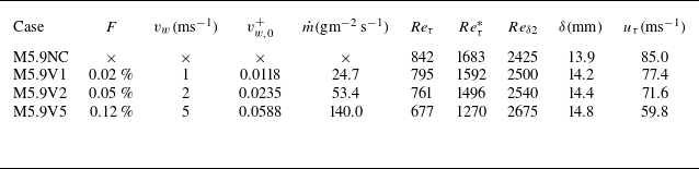
 Reτ=ρwuτδ/μw
 δ
δ 0.99
0.99 Reτ∗=ρuτ∗δ/μ
 uτ∗=τw/ρ
 vw,0+
vw,0+ uτ,0
uτ,0 m˙=ρwvw
 a
a M5.9NC
 b
b M5.9V1
 c
c M5.9V2
 d
d M5.9V5
 a
a M5.9NC
 M5.9V1
 M5.9V2
 M5.9V5
 b
b F
F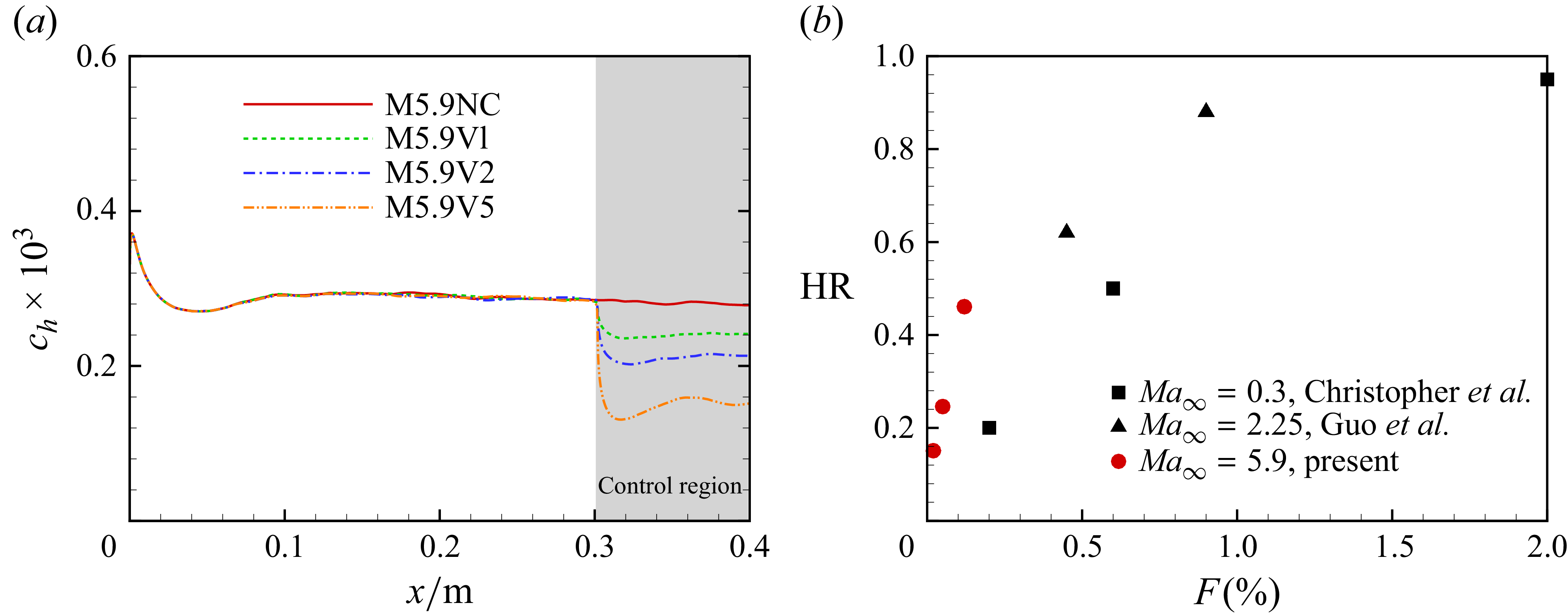
 a
a M5.9V1
 M5.9V2
 M5.9V5
 b
b F
F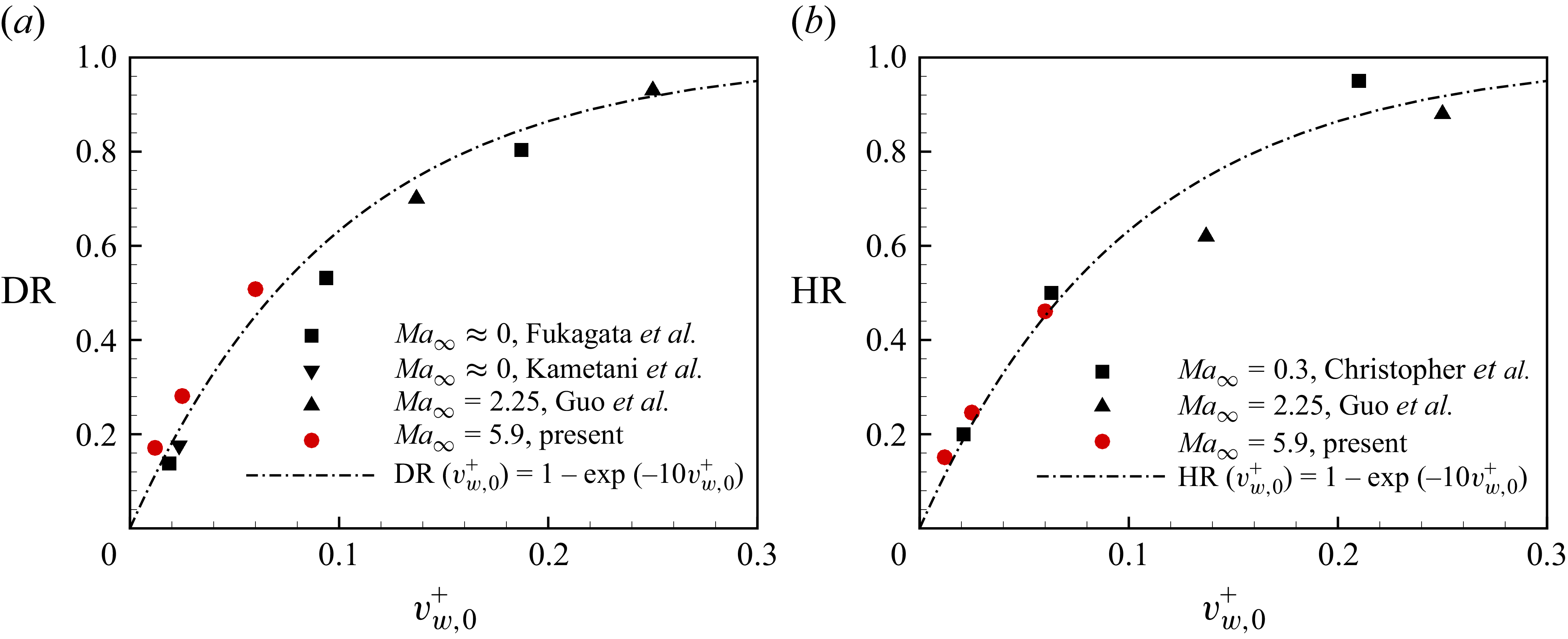
 a
a b
b
 a
a b
b c
c d
d
 Q
Q ×1011
×1011 T
T a
a b
b M5.9V1
 c
c M5.9V2
 d
d M5.9V5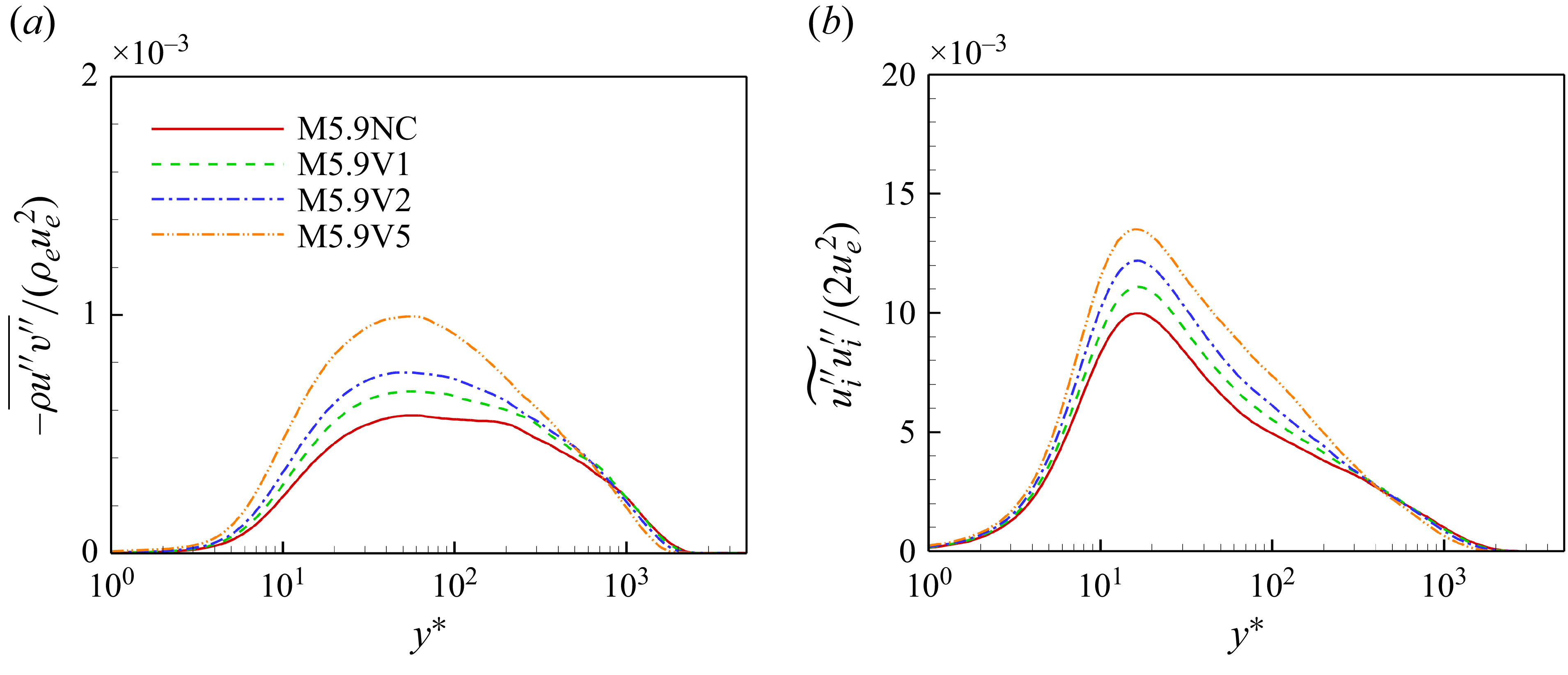
 a
a b
b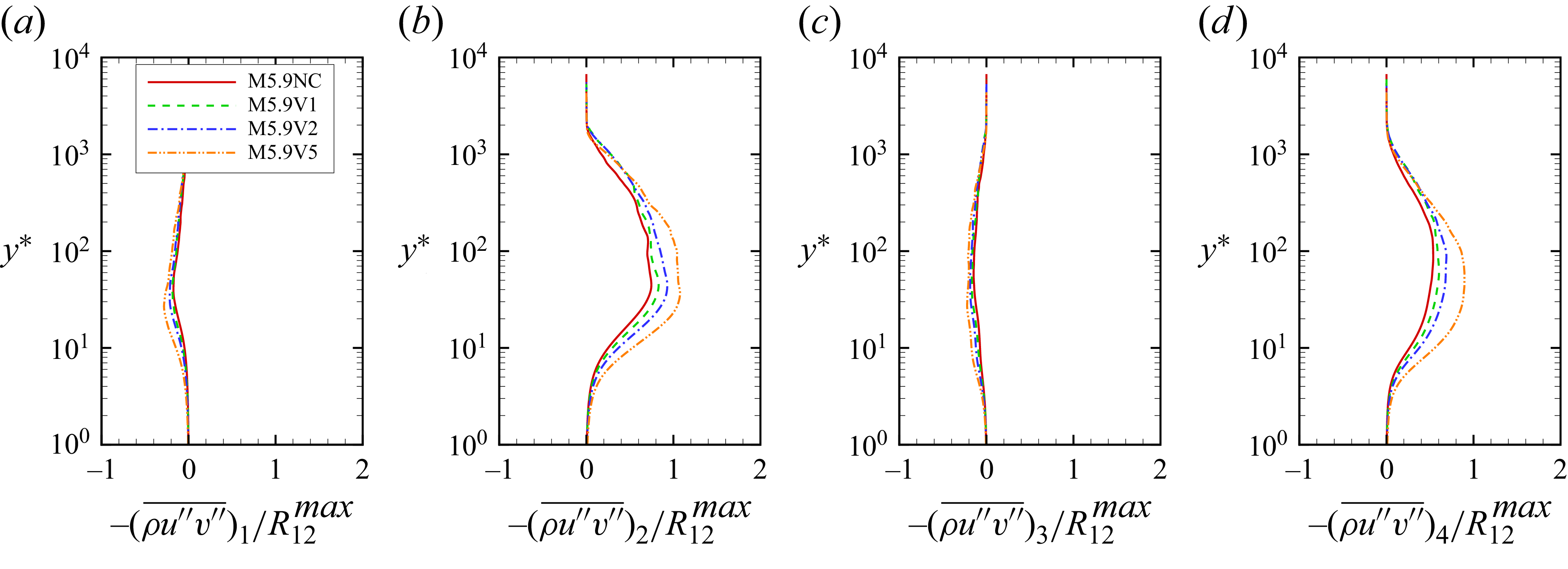
 a
a Q1
Q1 b
b Q2
Q2 c
c Q3
Q3 d
d Q4
Q4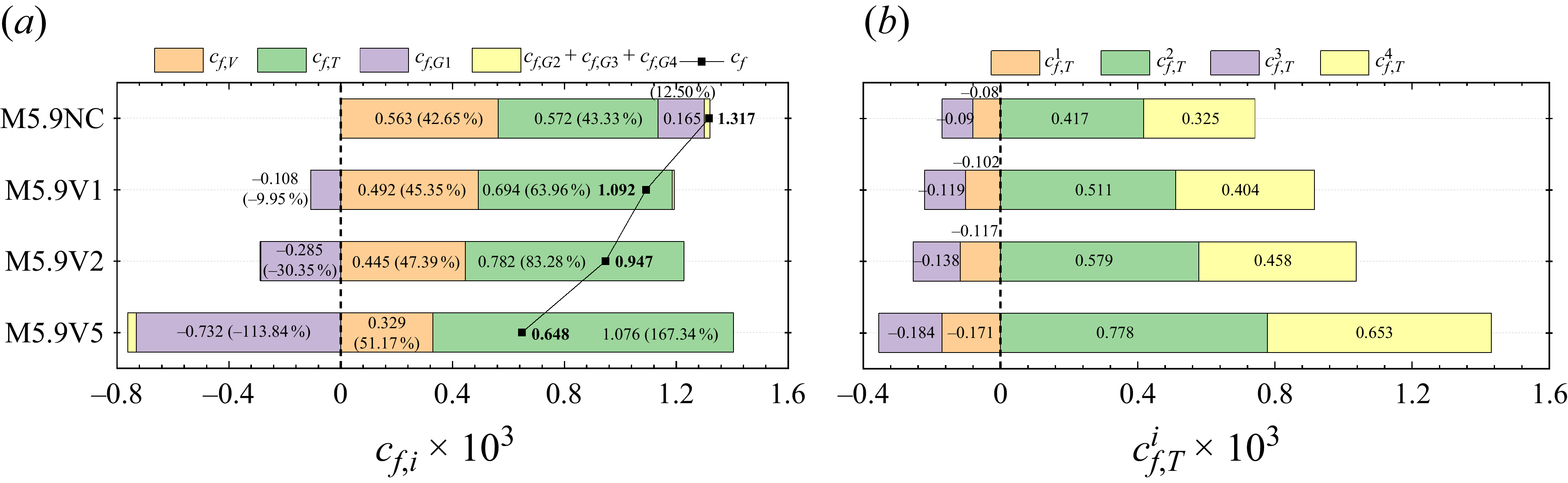
 a
a cf,V
cf,V cf,T
cf,T cf,G1
cf,G1 cf,G2+cf,G3+cf,G4
 b
b cf,T
cf,T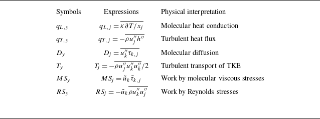

 a
a ch,V
ch,V ch,TH
ch,TH ch,D
ch,D ch,K
ch,K ch,MS
ch,MS ch,RS
ch,RS ch,G
ch,G b
b ch,RS
ch,RS
 v
v a
a y∗
y∗ b
b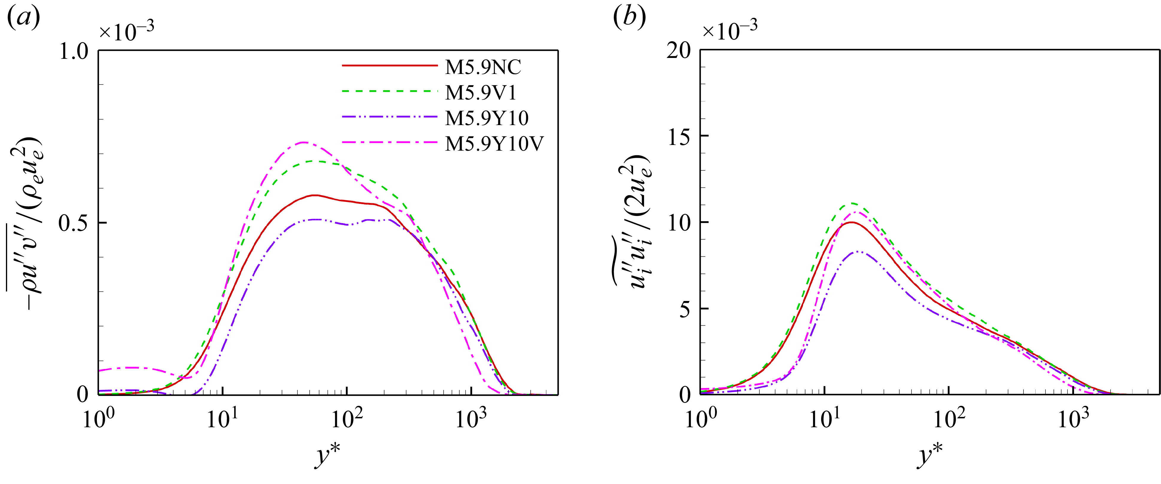
 a
a b
b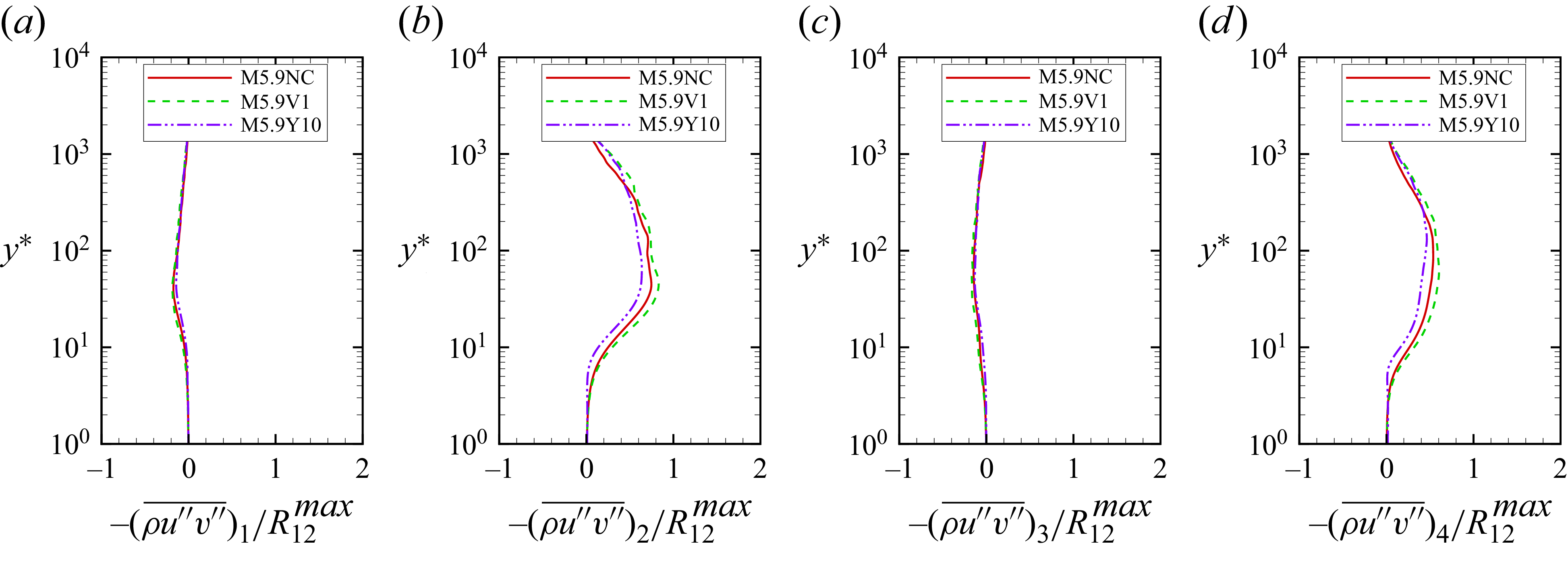
 a
a Q1
Q1 b
b Q2
Q2 c
c Q3
Q3 d
d Q4
Q4
 a
a b
b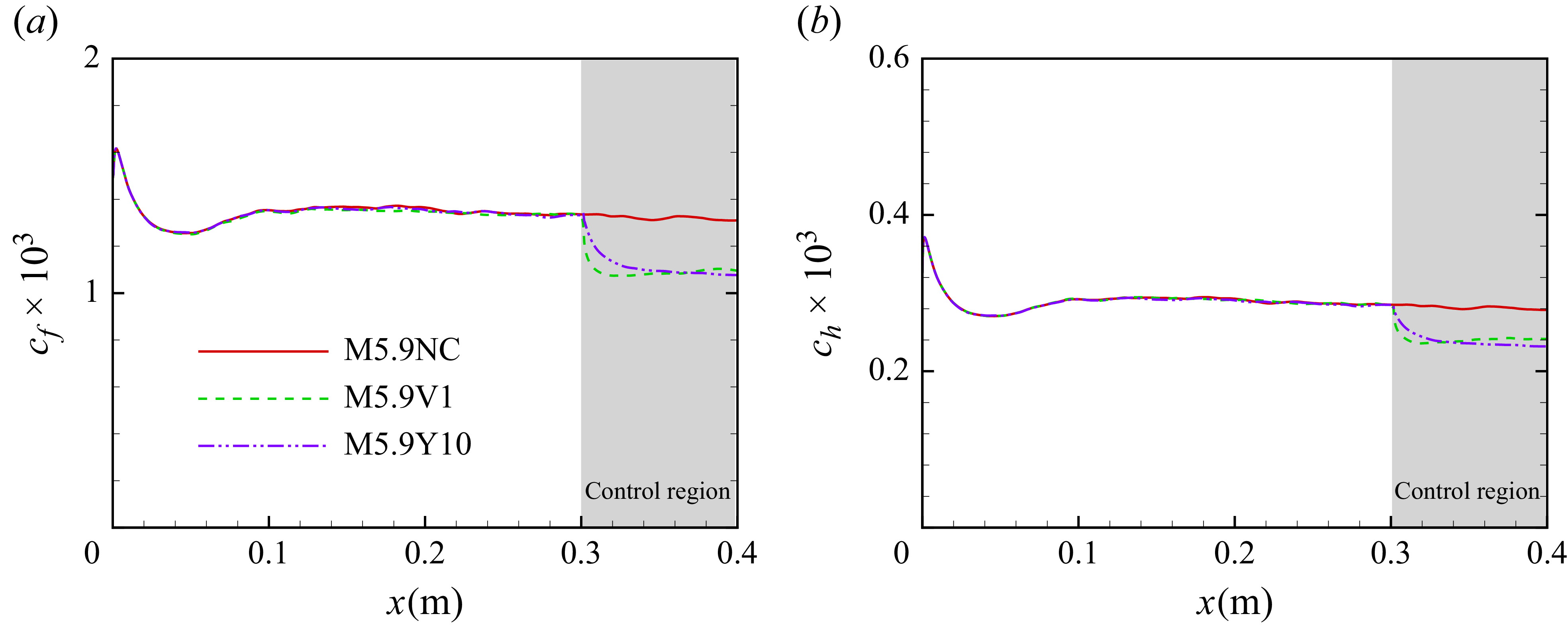
 a
a b
b M5.9V1
 M5.9Y10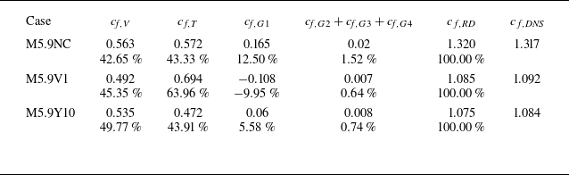
 ×103
×103 x
x cf,RD
cf,RD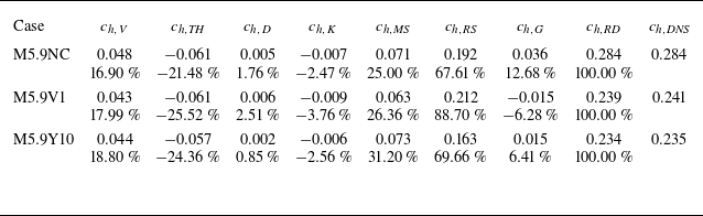
 ×103
×103 x
x ch,RD
ch,RD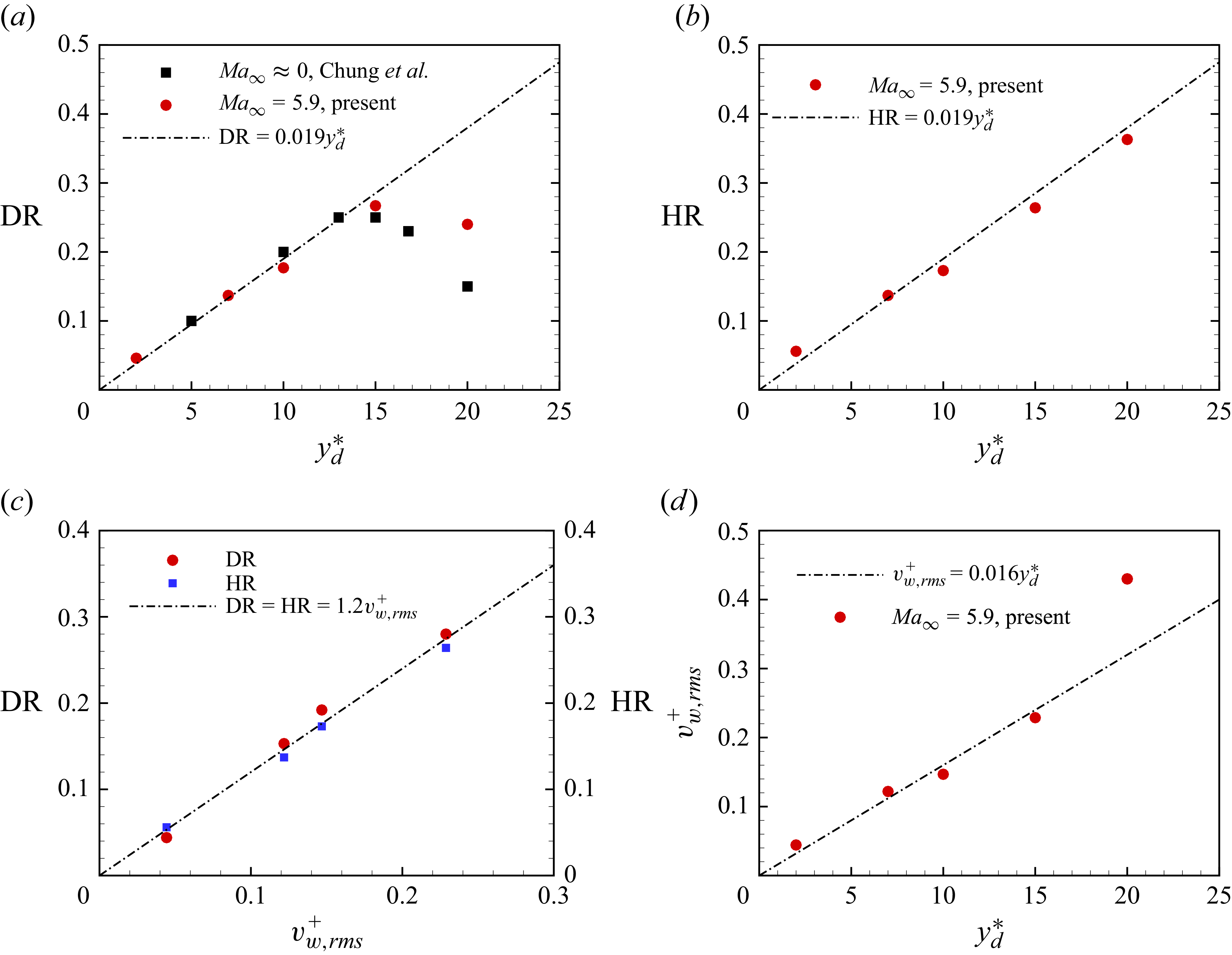
 a
a b
b yd∗
yd∗ c
c vw,rms+
 d
d vw,rms+
 yd∗
yd∗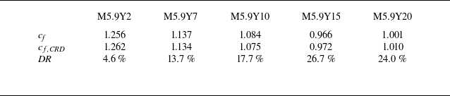
 ×103
×103 cf
cf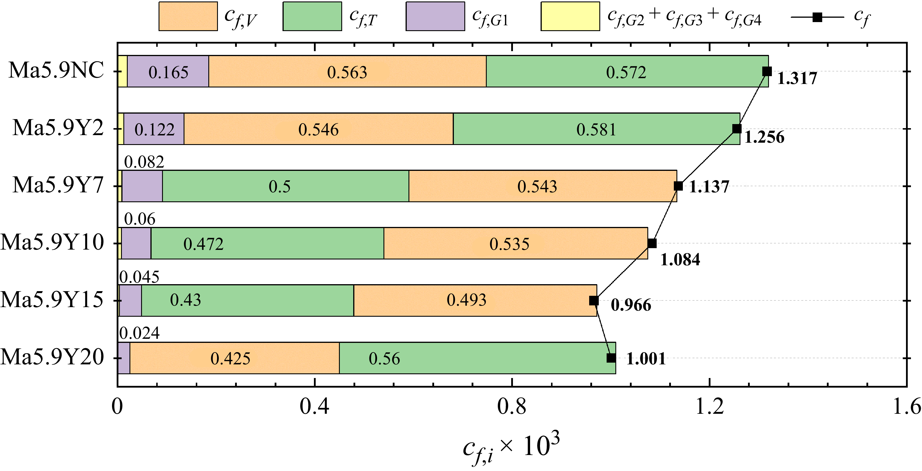

 ×103
×103 ch
ch
 cf,T
cf,T a−d
a−d ρeue2
ρeue2 a
a Q1
Q1 b
b Q2
Q2 c
c Q3
Q3 d
d Q4
Q4 e−h
e−h cf,T
cf,T e
e cf,T1
cf,T1 f
f cf,T2
cf,T2 g
g cf,T3
cf,T3 h
h cf,T4
cf,T4

 ch,RS
ch,RS a
a ch,RS1
 b
b ch,RS2
 c
c ch,RS3
 d
d ch,RS4
 ch,TH
ch,TH a
a d
d ρeueTe
 a
a Q1
Q1 b
b Q2
Q2 c
c Q3
Q3 d
d Q4
Q4 e−h
e−h ch,TH
ch,TH e
e ch,TH1
 f
f ch,TH2
 g
g ch,TH3
 h
h ch,TH4
 x
x z
z a
a y0∗
y0∗ M5.9Y10
 b
b y0∗
y0∗ M5.9Y20
 c
c x
x z
z d
d x
x z
z e
e y≈5×10⁻⁴
 a
a b
b c
c
 ×103
×103 x
x
 ×103
×103 x
x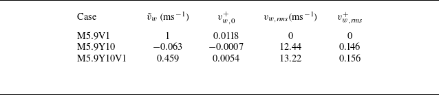
 x
x

 a
a cf
cf b
b ch
ch c
c −Rii
−Rii τw
τw d
d e
e f
f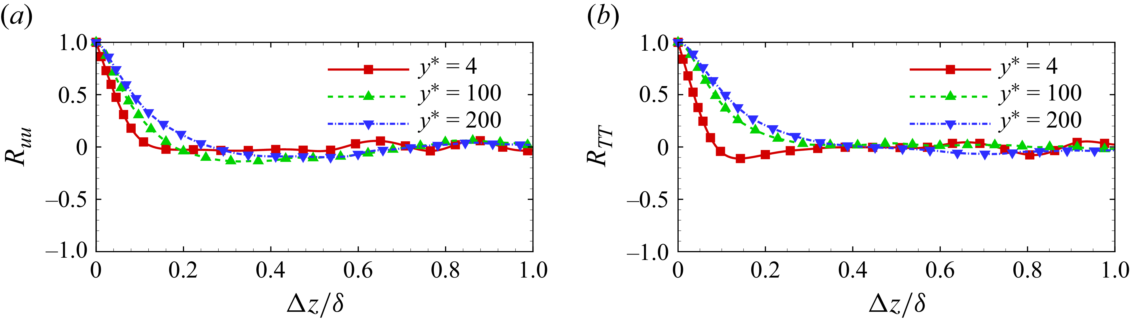
 a
a Ruu
Ruu b
b RTT
RTT Δz/δ
Δz/δ y∗
y∗ y∗
y∗ y∗
y∗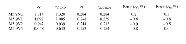
 (×103)
 x
x
 a,d
a,d M5.9V1
 b,e
b,e M5.9V2
 c,f
c,f M5.9V5
 cx
cx c
c
 a
a b
b

