


INTRODUCTION
During the final part of the Late Pleistocene (i.e., during Marine Oxygen Isotope Stage 2; 29–14 ka; Lisiecki and Raymo, Reference Lisiecki and Raymo2005), large ice sheets developed in Europe over Scandinavia and the British Isles. A network of valley glaciers covered the Alps at the same time. Previous work showed that ice build-up and decay followed complex temporal and spatial patterns (e.g., Ivy-Ochs et al., Reference Ivy-Ochs, Kerschner, Reuther, Preusser, Heine, Maisch, Kubik and Schlüchter2008; Hughes and Gibbard, Reference Hughes and Gibbard2015; Gaar et al., Reference Gaar, Graf and Preusser2019; Clark et al., Reference Clark, Ely, Hindmarsh, Bradley, Ignéczi, Fabel, Cofaigh and et al2022), apparently reflecting shifts of the position of the polar front over the North Atlantic (Florineth and Schlüchter, Reference Florineth and Schlüchter2000; Kuhlemann et al., Reference Kuhlemann, Rohling, Krumrei, Kubik, Ivy-Ochs and Kucera2008; Monegato et al., Reference Monegato, Scardia, Hajdas, Rizzini and Piccin2017; Gribenski et al., Reference Gribenski, Valla, Preusser, Roattino, Crouzet and Buoncristiani2021). Chronological data from moraines confirmed that, apart from these ice masses, ice caps and glaciers covered the currently ice-free, mid-elevation mountainous regions in Central Europe, including the Jura (Graf et al., Reference Graf, Akçar, Ivy-Ochs, Strasky, Kubik, Christl, Burkhard, Wieler and Schlüchter2015), the Vosges (Mercier et al., Reference Mercier, Bourlès, Kalvoda, Braucher and Paschen1999), the Black Forest (Hofmann et al., Reference Hofmann, Preusser, Schimmelpfennig and Léanni2022), the Bavarian Forest (Reuther, Reference Reuther2007), the Bohemian Forest (Mentlík et al., Reference Mentlík, Engel, Braucher, Léanni and Team2013), and the Giant Mountains (Mercier et al., Reference Mercier, Kalvoda, Bourlès, Braucher and Engel2000; Engel et al., Reference Engel, Traczyk, Braucher, Woronko and Křížek2011, Reference Engel, Braucher, Traczyk and Léanni2014). The highest peaks in these regions reach maximum elevations between 1424 m (Vosges) and 1720 m (Jura) above sea-level (note that elevations are given in meters above present-day sea-level throughout this paper). Episodes of abrupt cooling punctuated the warming trend during the last glacial termination (see Heiri et al., Reference Heiri, Koinig, Spötl, Barrett, Brauer, Drescher-Schneider and Gaar2014a, and Palacios et al., Reference Palacios, Hughes, García Ruiz and Andrés2023, for overviews), which was the period between the last glacial maximum (at 27.5–23.3 ka; Hughes and Gibbard, Reference Hughes and Gibbard2015) and the onset of the Holocene (at 11.7 ka; Rasmussen et al., Reference Rasmussen, Bigler, Blockley, Blunier, Buchardt, Clausen and Cvijanovic2014). These cooling events (at ca. 14 ka and ca. 12.7 ka) led to glacial re-advances and standstills in mid-elevation mountainous regions in Central Europe (Mercier et al., Reference Mercier, Bourlès, Kalvoda, Braucher and Paschen1999, Reference Mercier, Kalvoda, Bourlès, Braucher and Engel2000; Reuther, Reference Reuther2007; Engel et al., Reference Engel, Traczyk, Braucher, Woronko and Křížek2011, Reference Engel, Braucher, Traczyk and Léanni2014; Mentlík et al., Reference Mentlík, Engel, Braucher, Léanni and Team2013; Hofmann et al., Reference Hofmann, Preusser, Schimmelpfennig and Léanni2022).
Investigating past glaciations of mid-elevation mountainous regions in Central Europe (Fig. 1) may further refine our understanding of the mechanisms of Pleistocene climate change (cf., Heyman et al., Reference Heyman, Heyman, Fickert and Harbor2013). While the evolution of summer temperatures during the last glacial termination has been quantified at multiple sites in and around the Alps through the investigation of chironomid assemblages (e.g., Heiri and Millet, Reference Heiri and Millet2005; Larocque-Tobler et al., Reference Larocque-Tobler, Heiri and Wehrli2010; Heiri et al., Reference Heiri, Brooks, Renssen, Bedford, Hazekamp, Ilyashuk and Jeffers2014b; Bolland et al., Reference Bolland, Rey, Gobet, Tinner and Heiri2020), precipitation records are scarce (Guiot et al., Reference Guiot, Pons, Beaulieu and Reille1989; Magny et al., Reference Magny, Guiot and Schoellammer2001, Reference Magny, Aalbersberg, Bégeot, Benoit-Ruffaldi, Bossuet, Disnar and Heiri2006; Peyron et al., Reference Peyron, Bégeot, Brewer, Heiri, Magny, Millet, Ruffaldi, van Campo and Yu2005). Rea et al. (Reference Rea, Pellitero, Spagnolo, Hughes, Ivy-Ochs, Renssen, Ribolini, Bakke, Lukas and Braithwaite2020) attempted to fill this gap by conducting a reconstruction of precipitation during the 12.9–11.7 ka period, often referred to as the Younger Dryas (Mangerud, Reference Mangerud2021; Naughton et al., Reference Naughton, Sánchez-Goñi, Landais, Rodrigues, Riveiros, Toucanne, Palacios, Hughes, García Ruiz and Andrés2023). This reconstruction was based on temperature records from sites across Europe and on equilibrium-line altitudes (ELAs) of 122 glaciers (i.e., the zones of glaciers where net accumulation corresponded to net ablation over a period of one year; Bakke and Nesje, Reference Bakke, Nesje, Singh, Singh and Haritashya2011). Because ablation and accumulation are linked to the summer temperature and annual precipitation, respectively (Ohmura and Boettcher, Reference Ohmura and Boettcher2018), past precipitation at ELAs can be inferred with the aid of empirical relationships (Ohmura et al., Reference Ohmura, Kasser and Funk1992; Dahl et al., Reference Dahl, Nesje and Øvstedal1997; Ohmura and Boettcher, Reference Ohmura and Boettcher2018), if summer temperature estimates are available from an independent record. However, for Central Europe, the study of Rea et al. (Reference Rea, Pellitero, Spagnolo, Hughes, Ivy-Ochs, Renssen, Ribolini, Bakke, Lukas and Braithwaite2020) is limited to only one cirque glacier in the Giant Mountains. Although Rea et al. (Reference Rea, Pellitero, Spagnolo, Hughes, Ivy-Ochs, Renssen, Ribolini, Bakke, Lukas and Braithwaite2020) did not provide uncertainties for their precipitation estimates, the annual precipitation at the ELA of this glacier during the 12.9–11.7 ka period (1435 mm/yr) was in the range of present-day values (~1500 mm/yr-; Engel et al., Reference Engel, Braucher, Traczyk and Léanni2014). Interestingly, it is still unclear whether other mid-elevation mountainous regions in Central Europe, such as the Vosges or the Southern Black Forest, were also glaciated during this cool period. Furthermore, reconstruction of precipitation during other periods of the last glacial termination would enhance our understanding of past circulation changes but it would require additional data on the temporal and spatial evolution of glaciers and ELAs. Small ice masses are particularly suitable for precipitation reconstruction due to their short response times to climatic oscillations and their high sensitivity to short-term climatic changes (Mackintosh et al., Reference Mackintosh, Anderson and Pierrehumbert2017). However, topoclimatic factors, such as shading, may significantly influence their mass balance and need to be considered (e.g., Coleman et al., Reference Coleman, Carr and Parker2009; Mills et al., Reference Mills, Grab and Carr2009; Chandler and Lukas, Reference Chandler and Lukas2017).
Topographic map of Central Europe showing sites discussed in the text. The digital elevation model in the background is a SRTM–DEM (shuttle radar topography mission–digital elevation model; Jarvis et al., Reference Jarvis, Reuter, Nelson and Guevara2008). ©EuroGeographics for administrative boundaries. ©European Environment Agency for rivers and lakes.

The Black Forest is situated in southwestern Germany (Fig. 1) and is commonly subdivided into a northern, central, and southern part. During the last Pleistocene glaciation, the Northern Black Forest (max. elevation: 1164 m) hosted a small icefield and numerous cirque glaciers (Fezer et al., Reference Fezer, Günther and Reichelt1961; Zienert and Fezer, Reference Zienert and Fezer1967). Small cirque and valley glaciers covered areas at high elevation (max. elevation: ~1000 m) in the Central Black Forest (Reichelt, Reference Reichelt1996). Because a significant portion of the Southern Black Forest is situated above 1000 m, this region was the most extensively glaciated. Previous studies concluded that this region temporarily hosted four, presumably interconnected ice caps and their outlet glaciers, covering altogether an area of about 1000 km2 (Metz and Saurer, Reference Metz and Saurer2012). The largest ice cap rested on the highest summit, Feldberg (1493 m), and on the surrounding region (Fig. 2; cf., Hofmann et al., Reference Hofmann, Rauscher, McCreary, Bischoff and Preusser2020). The outlet glaciers of this ice cap attained lengths of up to 25 km and a maximum thickness of 440 m (Sawatzki, Reference Sawatzki1992; Hemmerle et al., Reference Hemmerle, May and Preusser2016). Three summits in the surrounding region (Belchen [1414 m], Köhlgarten [1224 m], and Schauinsland [1284 m]; Fig. 2) hosted significantly smaller ice caps (Giermann, Reference Giermann1964; Rahm, Reference Rahm1987).
Location of the study area and map of the study area showing sites discussed in the text. The assumed Late Pleistocene maximum ice extent in the Southern Black Forest (Hemmerle et al., Reference Hemmerle, May and Preusser2016) is shown in white. The DEM in the background was derived from data obtained during the SRTM (Earth Resources Observation and Science [EROS] Center, 2018). Photo locations/directions of view for Figure 3A–C shown as diagrammatic eyes.

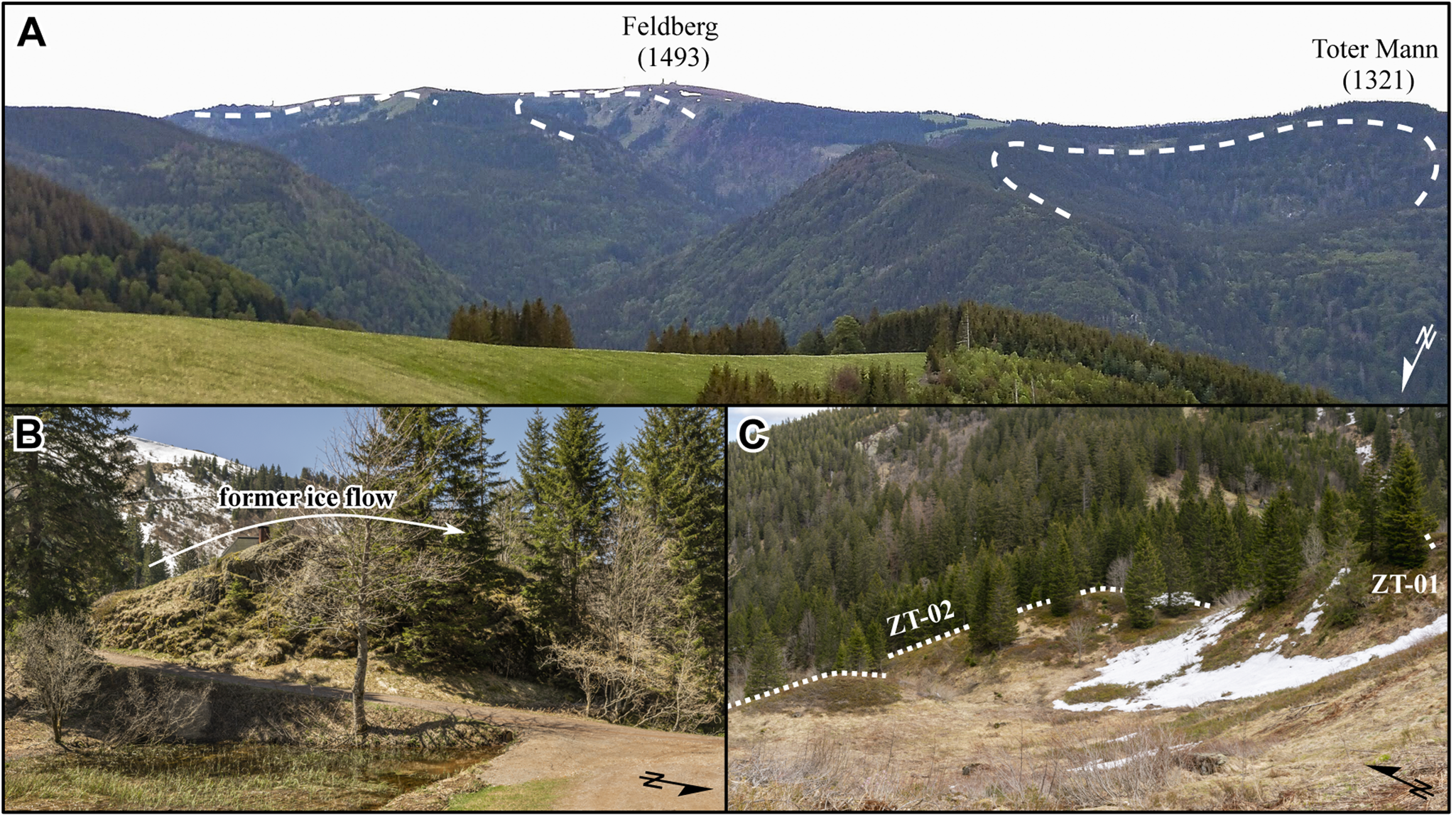
Examples of glacial landforms in the study area (elevations in m). (A) Panorama of the Zastler Tal Valley from Hinterwaldkopf. Three glacial cirques (marked with dashed lines) that are well recognizable from Hinterwaldkopf, from east to west, are the cirque in the upper reaches of the Sägenbachtal Valley, the stairway cirque in the uppermost part of the Zastler Tal Valley (Zastler Loch), and the Angelsbach Stairway Cirque. (B) Whaleback at an elevation of 1250 m in Zastler Loch. (C) Moraines at ice-marginal positions ZT-01 and ZT-02 (Hofmann et al., Reference Hofmann, Rauscher, McCreary, Bischoff and Preusser2020) seen from the western headwall of Zastler Loch. See Figure 2 for the locations and view directions from where photos were taken (all photos: F.M. Hofmann).
Numerous moraines have been mapped inside the assumed Late Pleistocene maximum ice extent around Feldberg, Belchen, Köhlgarten, and Schauinsland (Steinmann, Reference Steinmann1902; Liehl, Reference Liehl1982; Metz and Saurer, Reference Metz and Saurer2012). These landforms indicate that the ice caps first decayed into valley glaciers with independent accumulation areas and then evolved into small cirque glaciers (Hofmann et al., Reference Hofmann, Rauscher, McCreary, Bischoff and Preusser2020). 10Be CRE ages for moraines of one valley glacier suggest successive standstills and/or re-advances during overall glacier recession (between ca. 17 ka and ca. 16 ka), while final glacier recession in two cirques began no later than 14 ka (Hofmann et al., Reference Hofmann, Preusser, Schimmelpfennig and Léanni2022). Despite this recently published glacier chronology, Late Pleistocene glacier variations in the Southern Black Forest are not sufficiently understood for three reasons: (1) the onset of ice retreat from the last glaciation maximum position has not been dated (cf., Hofmann et al., Reference Hofmann, Preusser, Schimmelpfennig and Léanni2022), but this would answer the question if it occurred simultaneously with Alpine glaciers and the European ice shields; (2) it is not clear whether the deglaciation chronology presented by Hofmann et al. (Reference Hofmann, Preusser, Schimmelpfennig and Léanni2022) is representative for the entire Southern Black Forest; and (3) glacier variations at the end of the last deglaciation are poorly constrained because the presumably youngest moraines in the Black Forest have not been dated. These landforms are situated in the Zastler Tal Valley north of Feldberg. Lang (Reference Lang2005) speculated that these moraines might have the same age as those of the Egesen stadial in the Alps, exposure dated to 13.5–11 ka at multiple sites across the Alps (cf., Ivy-Ochs et al., Reference Ivy-Ochs, Monegato, Reitner, Palacios, Hughes, García Ruiz and Andrés2023).
For this study, previously mapped moraines in the Zastler Tal Valley and one of its tributary valleys were selected for 10Be CRE dating to elucidate the spatial and temporal evolution of the glaciers during the last glaciation of the Black Forest in more detail. This study aims to determine the onset of glacier recession from the moraines of the Late Pleistocene glaciation maximum and to test the hypothesis of Lang (Reference Lang2005) that the presumably youngest moraines have an age of about 13–11 ka. Determining their age has important implications for the reconstruction of precipitation patterns during the last cool period of the Pleistocene (12.9–11.7 ka). ELAs during moraine formation were reconstructed for use in tandem with previously published July temperature estimates for precipitation reconstruction.
STUDY AREA AND PREVIOUS WORK
Regional setting
The Zastler Tal Valley consists of the Zastler Tal Valley sensu stricto, hereinafter referred to as the main valley, and its tributary valleys, the Brumisbach Valley, Stollenbach Valley, Angelsbach Valley, Ahorndobel Valley, and the Rinkendobel Valley (Fig. 2). The uppermost reach of the main valley, referred to as Zastler Loch, is situated on the northeastern flank of Feldberg. The main valley meets the Bruggatal Valley at an elevation of about 450 m and leads into the Zarten Basin east of the city of Freiburg. The Hochfahrn–Toter Mann Massif separates the study area from the Sankt Wilhelmer Tal Valley to the southwest, whereas the Hinterwaldkopf Massif delimits the study area to the northeast. The entire study area drains to the Rhine.
The study area is located in the crystalline part of the Black Forest, representing the basement of the Variscan orogeny (380–290 Ma). With the denudation of the orogen, various sediments were deposited on top of the crystalline basement under terrestrial and marine conditions during the Permian, Triassic, and Jurassic (cf., Geyer and Gwinner, Reference Geyer and Gwinner2011). Due to tectonic activity associated with the formation of the Upper Rhine Graben (starting at around 50 Ma; Ziegler, Reference Ziegler1992), the Southern Black Forest was uplifted, and the Mesozoic sedimentary rocks were stripped off. Lithologies of the Variscan basement, such as migmatites, paragneisses, or orthogneisses, dominate the study area (Schreiner, Reference Schreiner1996).
A subarctic climate prevails in the summit area of Feldberg (Dfc climate according to the Köppen climate classification). According to data of the German Weather Service (DWD), mean annual precipitation and mean annual temperature from 1961–1990 CE amounted to 1909 mm and 3.3°C at the weather station on Feldberg (at 1486 m), respectively (https://opendata.dwd.de; accessed 22 June 2023). Snowfall accounts for about two-thirds of the annual precipitation (Parlow and Rosner, Reference Parlow, Rosner, Mäckel and Metz1997). Snow cover on Feldberg lasts, on average, for 157 days per year (Matzarakis, Reference Matzarakis2012). The climate at lower elevations than the summit area of Feldberg is classified as temperate (Cfb climate according to the Köppen climate classification). Elevation has a strong effect on the amount of annual precipitation, with mean annual precipitation increasing by 100 mm per 100 m in elevation (Parlow and Rosner, Reference Parlow, Rosner, Mäckel and Metz1997).
Ice-marginal positions in the Zastler Tal Valley
Widespread glacial landforms and deposits in the Zastler Tal Valley document the strong imprint of Quaternary glaciations (Wimmenauer et al., Reference Wimmenauer, Liehl and Schreiner1990; Hann et al., Reference Hann, Schreiner and Zedler2011; Metz and Saurer, Reference Metz and Saurer2012). Glaciers covered the main valley and probably four of its tributary valleys (the Brumisbach Valley, Stollenbach Valley, Angelsbach Valley, and the Rinkendobel Valley; Liehl, Reference Liehl1982). Prominent examples of erosional glacial landforms are the stairway cirque in the main valley (Zastler Loch), the Angelsbach Cirque, and a whaleback in Zastler Loch (Fig. 3).
Ice-marginal moraines occur at elevations between 550 m and 1430 m in the main valley as well as in two of its tributary valleys, the Angelsbach Valley and the Rinkendobel Valley. They were first mapped by Steinmann (Reference Steinmann1902, Reference Steinmann1910), whereas Erb (Reference Erb and Müller1948), Zienert (Reference Zienert1973), Liehl (Reference Liehl, Hofmann and Louis1975), and Schreiner (Reference Schreiner1977) identified additional moraines. Metz (Reference Metz1985a) later published a geomorphological map showing glacial landforms in the upper reaches of the study area. After the publication of two geological maps including the Zastler Tal Valley (Wimmenauer et al., Reference Wimmenauer, Liehl and Schreiner1990; Schreiner, Reference Schreiner1996), interest in the glaciation of the study area markedly declined. Previous work on moraines in the Zastler Tal Valley was summarized by Liehl (Reference Liehl1982), Metz and Saurer (Reference Metz and Saurer2012), Hemmerle et al. (Reference Hemmerle, May and Preusser2016), and Hofmann et al. (Reference Hofmann, Rauscher, McCreary, Bischoff and Preusser2020).
The availability of high-resolution elevation data has led to a renewed interest in glacial landforms in the study area. Geomorphological mapping was recently undertaken with the aid of such data (Hofmann et al., Reference Hofmann, Rauscher, McCreary, Bischoff and Preusser2020). Revisiting glacial landforms in the Zastler Tal Valley proved to be a prerequisite for this study because some of previously mapped moraines turned out to be landforms other than moraines, whereas some glacial landforms were mapped for the first time. Therefore, we refer to the study of Hofmann et al. (Reference Hofmann, Rauscher, McCreary, Bischoff and Preusser2020) in the following synthesis (see Fig. 4 for a map of moraines and ice-marginal positions).
Glacial cirques, moraine crests and ice-marginal positions in the (A) Zastler Tal Valley, the (B) Angelsbach Cirque, and the (C) uppermost part of the Zastler Tal Valley and in the Rinkendobel Valley (Hofmann et al., Reference Hofmann, Rauscher, McCreary, Bischoff and Preusser2020). See Figure 2 for the data source of the DEM in the background.

The lowermost ice-marginal landform in the main valley is a short sediment ridge on the southwestern valley wall at an elevation of 540–600 m (ZT-18; Fig. 4). It has been tentatively mapped as an ice-marginal moraine (Erb, Reference Erb and Müller1948; Hüttner, Reference Hüttner1967; Hofmann et al., Reference Hofmann, Rauscher, McCreary, Bischoff and Preusser2020). This landform has been considered indicative of the Late Pleistocene maximum ice extent in the Zastler Tal Valley (Fig. 2; Erb, Reference Erb and Müller1948; Liehl, Reference Liehl1982; Metz and Saurer, Reference Metz and Saurer2012). A nearby sediment ridge has been interpreted as an ice-marginal moraine and ascribed to ice-marginal position ZT-17.
A prominent ice-marginal moraine is located at the northwestern end of a tongue basin farther upvalley (ice-marginal position ZT-16). According to Zienert (Reference Zienert1973), this moraine represents the Late Pleistocene glaciation maximum in the Zastler Tal Valley. A ridge-shaped accumulation of boulders on the northeast-facing valley wall between the entrance to the Stollenbach Valley and Angelsbach Valley probably pertains to the same ice-marginal position (Hofmann et al., Reference Hofmann, Rauscher, McCreary, Bischoff and Preusser2020, Fig. 13).
The moraines atice-marginal position ZT-15 are situated at around 640 m. A small ice-marginal moraine farther upvalley (at 720 m) documents ice-marginal position ZT-14. Two ice-marginal moraines are situated on the western valley wall near the entrance to the Rinkendobel Valley (ice-marginal positions ZT-13 and ZT-12). Two moraines on the eastern valley wall probably belong to the same ice-marginal positions (Fig. 4C). Two smooth moraines lie on the valley floor (ice-marginal positions ZT-11 and ZT-10). These moraines have been considered as old as two moraines on the eastern valley wall farther southeast (Fig. 4C).
The morphologically most prominent ice-marginal moraine in the entire main valley is a semi-circular, double-crested moraine complex at an elevation of 1030 m (at ice-marginal positions ZT-09 and ZT-08). The eastern part of the moraine complex is oriented parallel to the valley floor and progresses in a southerly direction farther upvalley.
An ice-marginal moraine is situated farther southeast on the eastern valley wall high above the valley floor (ice-marginal position ZT-07). An ice-marginal moraine on the eastern valley wall and a moraine on the opposite valley wall have been ascribed to the next younger ice-marginal position ZT-06. Two rather small ice-marginal moraines lie on the eastern valley wall farther southeast. These landforms probably pertain to ice-marginal positions ZT-08 and ZT-05. The ice-marginal moraines at ice-marginal position ZT-04 are situated on the lowermost cirque floor of Zastler Loch. Lang (Reference Lang2005) correlated the moraines at ice-marginal positions ZT-04 and younger moraines with those ascribed to the Egesen stadial in the Alps (exposure dated to 13.5–11 ka; Ivy-Ochs et al., Reference Ivy-Ochs, Monegato, Reitner, Palacios, Hughes, García Ruiz and Andrés2023).
An ice-marginal moraine is located at an elevation of 1340–1350 m on the western headwall of Zastler Loch. This landform is probably as old as an ice-marginal moraine farther east, hence these landforms are considered indicative of ice-marginal position ZT-03. The geometries of the crests of all moraines in younger morphostratigraphic positions (ice-marginal positions ZT-02 and ZT-01) suggest that the moraines formed at the margin of two different glaciers. A lobate series of ice-marginal moraines at 1320–1340 m documents ice-marginal position ZT-02 of a small glacier on the cirque's western headwall. The innermost ice-marginal position ZT-01 at this locality is documented by small ice-marginal moraines. Another set of moraines is situated on the uppermost cirque floor farther southeast (at 1400–1430 m). The moraines on the uppermost cirque floor (ice-marginal positions ZT-02 and ZT-01) are located at a significantly higher elevation than those on the western headwall.
Numerous moraines have been mapped in the Rinkendobel Valley and on the main ridge between the Rinkendobel Valley and the upper part of the Zastler Tal Valley. Because till covers the southward-facing slope north of Rinken Pass up to an elevation of 1240 m (Metz, Reference Metz1985b; Wimmenauer et al., Reference Wimmenauer, Liehl and Schreiner1990; Schreiner, Reference Schreiner1996), the moraines probably formed at the margin of an ice stream that advanced from the Sägenbachtal Valley over Rinken Pass into the Rinkendobel Valley. The lobate moraine in the southern glacial cirque west of Rinken Pass probably formed at the margin of a small cirque glacier (Liehl, Reference Liehl, Hofmann and Louis1975; Metz, Reference Metz1985b).
The moraines in the Angelsbach Valley have been assigned to five ice-marginal positions (Fig. 4B). The moraine at ice-marginal position AB-05 is situated on the eastern valley wall. A double-crested moraine complex on the valley floor documents ice-marginal positions AB-04 and AB-03. This landform is probably as old as two ice-marginal moraines on the eastern valley wall farther south. The morphologically most prominent glacial landforms in the Angelsbach Cirque, the moraines at ice-marginal position AB-02, are situated farther upvalley. These moraines surround Heibeermoos, a peat bog in the former tongue basin in the Angelsbach Cirque (Fig. 4; Erb, Reference Erb and Müller1948; Hann et al., Reference Hann, Schreiner and Zedler2011). An ice-marginal moraine is situated at the northern end of the southernmost cirque in the Angelsbach Valley. This landform documents ice-marginal position AB-01. Although initial cirques have been mapped in the upper reaches of the Stollenbach Valley and the Brumisbach Valley (Hofmann et al., Reference Hofmann, Rauscher, McCreary, Bischoff and Preusser2020), these valleys are devoid of ice-marginal landforms.
METHODS
10Be CRE dating
Fieldwork
During geomorphological field mapping for an earlier study (Hofmann et al., Reference Hofmann, Rauscher, McCreary, Bischoff and Preusser2020), all suitable moraine boulders with a height of ≥ 1 m observed in the main valley as well as in the Angelsbach Cirque were sampled for 10Be CRE dating. In an attempt to avoid complex exposure histories, we only selected boulders that were well embedded in moraines. Most of these boulders were not flat-topped, thus inclined rock surfaces with a constant angle were chosen. Rock surfaces near edges were avoided to prevent potential edge effects (Masarik and Wieler, Reference Masarik and Wieler2003). The strike and dip of the selected sampling surfaces were recorded with a geological compass. The coordinates of sampling sites were determined with a handheld GPS. Rock samples (n = 18; Table 1) were obtained with the aid of a battery-powered saw and a chisel. A detailed sample documentation is given in the supplementary material.
Characteristics of samples from moraine boulders in the Zastler Tal Valley. Sample numbers from the moraine boulders refer to the morphostratigraphic positions of the respective ice-marginal moraines.

Sample preparation and accelerator mass spectrometry measurements
Prior to sample preparation, the mass and thickness of each rock fragment in a sample was determined to compute the mass-weighted average of the sample's thickness. Quartz separation and 10Be extraction from purified quartz were conducted in the laboratory facilities of the University of Freiburg (Germany) and the Laboratoire National des Nucléides Cosmogéniques (LN2C) in Aix-en-Provence (France) according to a protocol adapted from Brown et al. (Reference Brown, Edmond, Raisbeck, Yiou, Kurz and Brook1991) and Merchel and Herpers (Reference Merchel and Herpers1999). After crushing, and wet sieving, the samples were passed through a magnetic separator (S.G. Frantz Co.). The samples were then treated with mixtures of 37% HCl and 35% H2SiF6 to further isolate quartz and remove feldspars. Because the samples still contained feldspar after this treatment, they were etched with diluted 5.5% HF, dried, spiked with magnetite powder (325 mesh) and passed through a magnetic separator. Atmospheric 10Be was removed with 48% HF in three steps. In each step, 10% of the quartz was dissolved. About 150 mg of a 9Be carrier solution (3025 ± 9 μg 9Be/g) was added to each sample before total dissolution with 48% HF. Chromatography with anionic and cationic exchange resins (DOWEX 1X8 and 50WX8), as well as precipitation stages subsequently were conducted to further separate and purify beryllium. The final Be(OH)2 precipitate was dried and oxidized at 700°C to obtain BeO.
Beryllium oxide was mixed with niobium powder and loaded into copper cathodes for accelerator mass spectrometry (AMS) measurements. AMS measurements were performed at the French national facility ASTER (Accélérateur pour les Sciences de la Terre, Environnement, Risques; Arnold et al., Reference Arnold, Merchel, Bourlès, Braucher, Benedetti, Finkel, Aumaître, Gottdang and Klein2010) at CEREGE (Centre Européen de Recherche et d'Enseignement des Geosciences de l'Environnement) in Aix-en-Provence, France. Measured 10Be/9Be ratios were normalized with respect to the in-house standard STD-11 using an assigned 10Be/9Be ratio of (1.191 ± 0.013) × 10−11 (Braucher et al., Reference Braucher, Guillou, Bourlès, Arnold, Aumaître, Keddadouche and Nottoli2015) and the 10Be half-life of (1.387 ± 0.012) × 106 years (Chmeleff et al., Reference Chmeleff, Blanckenburg, Kossert and Jakob2010; Korschinek et al., Reference Korschinek, Bergmaier, Faestermann, Gerstmann, Knie, Rugel and Wallner2010). It should be noted that the STD-11 standard was calibrated by reference to the NIST_27900 standardization that is equivalent to the widely used KNSTD07 standardization (Nishiizumi et al., Reference Nishiizumi, Imamura, Caffee, Southon, Finkel and McAninch2007) at rounding error (https://hess.ess.washington.edu/math/docs/al_be_v22/AlBe_standardization_table.pdf; accessed 30 June 2023). The 10Be/9Be ratio uncertainty in Table 2 includes the measurement uncertainty (counting statistics), the uncertainty of average standard measures, and the systematic error of ASTER (0.5%; Arnold et al., Reference Arnold, Merchel, Bourlès, Braucher, Benedetti, Finkel, Aumaître, Gottdang and Klein2010). 10Be concentrations in rock samples (Table 2) were corrected with the 10Be concentration in a batch-specific chemical blank (measured 10Be/9Be ratio: [0.125 ± 0.021] × 1014; number of added 9Be atoms: [2.98355 ± 0.02208] × 1019; 10Be concentration: 37264 ± 6365 atoms 10Be).
Results of Be measurements and cosmic-ray exposure ages of moraine boulders in the Angelsbach Cirque (AB) and in the Zastler Tal Valley sensu stricto (ZT). 10Be concentrations in samples were corrected with the 10Be concentration in a batch-specific chemical blank (37,264 ± 6365 atoms 10Be). *During AMS measurements, 9Be currents strongly decreased from 3.8 μA to 0.2 μA, therefore the age should not be considered reliable. **During Be measurements, Be currents dropped from 1.6 μA to 0.3 μA, therefore the age stated here should not be considered robust.

CRE age calculations
The elevations of the sampling sites were retrieved from a digital elevation model of the study area with x-y resolution of 1 m derived from light detection and ranging (LiDAR) data of the Baden–Württemberg State Agency for Spatial Information and Rural Development. Topographic shielding is commonly determined by approximating the horizon with a series of points and straight lines between them. Pairs of azimuth and elevation angles are recorded with an inclinometer as well as a compass and subsequently converted into a shielding factor (Li, Reference Li2013, Reference Li2018; Hofmann, Reference Hofmann, Preusser, Schimmelpfennig and Léanni2022). This approach could not be applied to most sampling sites in the study area because most boulders were situated in dense forests where the horizon was not visible. Therefore, topographic shielding factors were computed with an ArcGIS toolbox (Li, Reference Li2018). As recommended by Hofmann (Reference Hofmann2022), the high-resolution digital elevation model was resampled to x-y resolution of 30 m for shielding factor calculations.
Apparent CRE ages in ka (kiloyears before 2010 CE) as well as internal (analytical) and external uncertainties (analytical uncertainties plus the error of the 10Be production rate added in quadrature) were calculated with the online cosmic-ray exposure program (CREp; Martin et al., Reference Martin, Blard, Balco, Lavé, Delunel, Lifton and Laurent2017), which is available at https://crep.otelo.univ-lorraine.fr (accessed 16 May 2022). The 10Be production rate deduced from rock samples of the Chironico landslide in southern Switzerland (Claude et al., Reference Claude, Ivy-Ochs, Kober, Antognini, Salcher and Kubik2014) was selected because the landslide was the closest production-rate reference site to the study area. Time-dependent ‘Lm’ scaling (Nishiizumi et al., Reference Nishiizumi, Winterer, Kohl, Klein, Middleton, Lal and Arnold1989; Lal, Reference Lal1991; Stone, Reference Stone2000; Balco et al., Reference Balco, Stone, Lifton and Dunai2008) and the ERA atmosphere model (Uppala et al., Reference Uppala, Kållberg, Simmons, Andrae, Da Bechtold, Fiorino and Gibson2005), as recommended by Martin et al. (Reference Martin, Blard, Balco, Lavé, Delunel, Lifton and Laurent2017), were selected in CREp to scale the 10Be production rate to sampling sites. The ages were corrected for changes in Earth's magnetic field with data from an atmospheric 10Be-based geomagnetic database (Muscheler et al., Reference Muscheler, Beer, Kubik and Synal2005). Selecting these parameters led to a production rate of 4.10 ± 0.10 atoms 10Be/g quartz/yr at sea-level and high latitudes (SLHL), thus concurring with the global production rate in CREp (4.11 ± 0.19 atoms 10Be/g quartz/yr at SLHL). Since the sampled boulders were quartz rich, the density of quartz (2.65 g/cm3) was assumed to perform the thickness correction.
Because no protruding quartz veins were observed on the sampled boulders, we were unable to calculate sampling site-specific denudation rates for CRE age calculations. Reuther (Reference Reuther2007) proposed a denudation rate of 0.24 cm/ka for a similar lithological and environmental setting in the Bavarian Forest (Fig. 1; recalculated with CREp and the parameters listed previously). Incorporating this (recalculated) denudation rate yielded, on average, 2.7% older ages. The age difference was largest for the ZT-15a-1 boulder (3.4%).
The 10Be production rate from the Chironico landslide is affected by snow-cover bias but is not accounted in CREp. Because almost all sampling sites in the study area lie at a much higher elevation than the Chironico landslide (~800 m), snow cover is likely more important for our study. According to field observations, the sampled boulders were covered in winter by a few decimeters of snow, which is not easily removed by wind in forested areas. According to data from the weather station of the German Weather Service in the municipality of Titisee (at 846 m), situated east of the study area, seasonal snow cover lasted, on average, for four months in the 1961–1990 CE period (average snow thickness : 30 cm). Assuming similar snow cover on the sampled boulders during the whole duration of exposure, a snow density of 0.3 g/cm3, an attenuation length for fast neutrons in snow of 109 g/cm2 (Zweck et al., Reference Zweck, Zreda and Desilets2013), and the commonly used equation 3.76 of Gosse and Phillips (Reference Gosse and Phillips2001), an additional snow shielding factor of ~0.974 is suggested. Incorporating this factor during age calculations yields ages older by 2.6% on average.
Correcting the ages for both denudation and snow shielding leads to ages that are older by 5.4% on average (Table 2). These considerations imply that the ages presented here may be underestimated by a few centuries. However, because we cannot prove that the corrections for snow shielding and postglacial denudation are correct, we present both uncorrected (minimum estimate) and corrected exposure ages (Table 2).
Statistical assessment of ages
Where possible, multiple boulders were sampled at individual ice-marginal positions to detect potential under- and overestimated ages. The assessment of ages follows the procedure in Hofmann et al. (Reference Hofmann, Preusser, Schimmelpfennig and Léanni2022): if three or more ages were available from the same landform, reduced chi-squared ($\chi ^2_R$ ) was computed. $\chi ^2_R$
 was compared with a critical value from a standard χ 2-table (degrees of freedom = n–1). The confidence interval was set to 95%. If $\chi ^2_R$
 was lower than the critical value, the hypothesis that the data form a single population is at 95% confidence (Balco, Reference Balco2011). In this case, the landform age corresponds to the arithmetic mean of the ages. The mean internal uncertainty of the ages plus the production rate error added in quadrature was defined as landform age uncertainty. If $\chi ^2_R$
 exceeded the critical value, measurement uncertainties did not fully account for scatter in ages from the same landform (Balco, Reference Balco2011). In this case, the age that was farthest from the average age in relation to its measurement uncertainty was considered an outlier. This procedure was repeated until the remaining ages yielded an acceptable $\chi ^2_R$
 value. No more than half of the ages from the same landform were excluded. The landform age was determined by calculating the arithmetic mean of the remaining ages. The landform age uncertainty corresponds to the mean internal uncertainty of the remaining ages and the production rate error (2.4%) added in quadrature.
Glacier reconstructions and ELA calculations
Reconstructing ELAs of a former glacier provides valuable insights into the paleoclimate if the glacier's mass balance was predominantly controlled by temperature and precipitation (Mackintosh et al., Reference Mackintosh, Anderson and Pierrehumbert2017). Common methods for reconstructing ELAs are the accumulation area ratio (AAR) and the area–altitude balance ratio (AABR) methods (Pearce et al., Reference Pearce, Ely, Barr, Boston, Clarke and Nield2017). In contrast to the former, the latter explicitly takes the hypsometry of a glacier into account (Osmaston, Reference Osmaston2005) and was therefore adopted for this study.
This approach required glacier-surface reconstructions. For establishing DEMs of former glacier surfaces, the GlaRe toolbox for the ESRI ArcGIS software was chosen (Pellitero et al., Reference Pellitero, Rea, Spagnolo, Bakke, Ivy-Ochs, Frew, Hughes, Ribolini, Lukas and Renssen2016). For the first step, flowlines of former glaciers were created in ArcMap 10.8.1 and points with a spacing of 50 m were created along the flowlines. To calculate ice thickness, the basal shear stress needed to be provided at these points. Pellitero et al. (Reference Pellitero, Rea, Spagnolo, Bakke, Ivy-Ochs, Frew, Hughes, Ribolini, Lukas and Renssen2016) suggested adjusting the basal shear stress progressively until the reconstructed ice thickness agrees with the position of ice-marginal landforms, such as moraines. In most cases, ice-marginal landforms have only been preserved close to former positions of glacier fronts. In these areas, the basal shear stress could be adjusted to tune glacier surfaces to geomorphological evidence. In all remaining areas, the default value of the GlaRe toolbox was used (100,000 Pa).
In topographically constrained areas, resistance to glacier flow can be provided by lateral drag (Benn and Hulton, Reference Benn and Hulton2010). Dimensionless shape factors (f) for points in topographically constrained areas were deduced from automatically created cross sections and ice thicknesses were recalculated. Contour lines of modern surfaces were derived from a resampled version of the high-resolution digital terrain model of the study area (x-y resolution = 5 m). Contour lines of former glaciers were drawn by hand. Following the approach of Sissons (Reference Sissons1974), concave and convex contour lines were drawn in the suspected accumulation and ablation areas, respectively. DEMs of former glacier surfaces were established by applying the ‘from contour to DEM’ tool in the ELA calculation toolbox of Pellitero et al. (Reference Pellitero, Rea, Spagnolo, Bakke, Hughes, Ivy-Ochs, Lukas and Ribolini2015).
In an earlier study on the Late Pleistocene glaciation of the Southern Black Forest (Hofmann et al., Reference Hofmann, Preusser, Schimmelpfennig and Léanni2022), ELAs were calculated with balance ratios for the Alps. Since we aimed to reconstruct annual precipitation at the ELA based on a precipitation/temperature function derived from data from modern glaciers across the world, ELAs were calculated with the global AABR to ensure consistency. Oien et al. (Reference Oien, Rea, Spagnolo, Barr and Bingham2022) demonstrated that the mean global AABR (1.75; presented by Rea, Reference Rea2009) is statistically invalid and proposed that the median global AABR of 1.56 should be used for ELA calculations. Therefore, ELAs in the study area were calculated with a balance ratio of 1.56. The recently published AABR–ELAs of former glaciers in the Southern Black Forest (Hofmann et al., Reference Hofmann, Preusser, Schimmelpfennig and Léanni2022) that were calculated with a balance ratio of 1.59 were recalculated with the median global AABR, leading to subtle shifts in ELAs.
Oien et al. (Reference Oien, Rea, Spagnolo, Barr and Bingham2022) found that the absolute median difference between ELAs calculated with the median global balance ratio and the actual ELAs of glaciers across the world amounts to 65.5 m. They argued that this difference can be regarded as potential error associated with calculated AABR–ELAs. The error of the ELA calculation is half of the interval chosen for ELA calculations (Pellitero et al., Reference Pellitero, Rea, Spagnolo, Bakke, Hughes, Ivy-Ochs, Lukas and Ribolini2015). Because the interval was set to 2 m for this study, the error of the ELAs amounts to 1 m. This value and the potential error associated with the calculated AABR–ELAs were added in quadrature to determine the total ELA uncertainty. It should be noted that total ELA uncertainties only comprise the error associated with the AABR method.
ELA-based precipitation reconstruction
According to a global dataset compiled by Ohmura and Boettcher (Reference Ohmura and Boettcher2018), winter accumulation plus summer precipitation (Pa) in mm/yr at the ELA is related to the 3-month summer temperature (T3) in the free atmosphere (°C) (i.e., the June, July, and August temperature in the northern hemisphere) which is:

The standard error of this relationship amounts to 648 mm/yr (Ohmura and Boettcher, Reference Ohmura and Boettcher2018).
The suitability of temperature/precipitation (P/T) relationships at ELAs of modern glaciers for formerly glaciated areas has been vigorously debated (e.g., Golledge et al., Reference Golledge, Hubbard and Sugden2008, Reference Golledge, Hubbard and Bradwell2010; Boston et al., Reference Boston, Lukas and Carr2015; Chandler et al., Reference Chandler, Boston and Lukas2019). Golledge et al. (Reference Golledge, Hubbard and Sugden2008, Reference Golledge, Hubbard and Bradwell2010) argued that the P/T function of Ohmura et al. (Reference Ohmura, Kasser and Funk1992) ignores the principle of continentality. Indeed, the equations of both Ohmura et al. (Reference Ohmura, Kasser and Funk1992) and Ohmura and Boettcher (Reference Ohmura and Boettcher2018) were derived from a global dataset of glaciers in various climatic regimes, including strongly maritime and continental Arctic settings. Increased seasonality results in a shorter ablation season (Hughes and Braithwaite, Reference Hughes and Braithwaite2008), hence both equations will lead to an overestimation of accumulation or precipitation in settings with a highly continental climate. Climatic reconstructions point to extreme seasonality in Europe during the last glacial termination (Isarin and Renssen, Reference Isarin and Renssen1999; Renssen and Isarin, Reference Renssen and Isarin2001; Denton et al., Reference Denton, Alley, Comer and Broecker2005, Reference Denton, Anderson, Toggweiler, Edwards, Schaefer and Putnam2010; Schenk et al., Reference Schenk, Väliranta, Muschitiello, Tarasov, Heikkilä, Björck, Brandefelt, Johansson, Näslund and Wohlfarth2018). To the best of our knowledge, no relationship between summer temperatures and precipitation at the ELA has been proposed for the last glacial termination in Central Europe. Owing to the lack of a suitable alternative, the equation of Ohmura and Boettcher (Reference Ohmura and Boettcher2018) was adopted for this study.
Unfortunately, no July temperature record is available for the last glacial termination in the Black Forest. The closest site to the study area for which July temperatures have been inferred from chironomid assemblages is Burgäschisee on the Swiss Plateau (situated ~80 km south-southwest of the study area; Fig. 1). The recently published Burgäschisee July temperature record (Bolland et al., Reference Bolland, Rey, Gobet, Tinner and Heiri2020) encompasses the period from ca. 18.4 ka to ca. 14.1 ka. The July temperature reconstruction for Lac Lautret (Jura; Fig. 1) for the 16.0–11.1 ka period (Heiri and Millet, Reference Heiri and Millet2005) was not used for two reasons. First, the reconstructed July temperatures for both sites (adjusted to an elevation of 1000 m assuming a lapse rate of 0.007 K/m; Kuttler, Reference Kuttler2013) differ significantly in the 16.0–14.1 ka period, with an offset of up to ~5°C. As discussed by Heiri et al. (Reference Heiri, Ilyashuk, Millet, Samartin and Lotter2015), this offset might be due to microclimatological/topographical effects that are known to affect water temperatures of lakes or regional differences in temperatures. Second, Lac Lautret is located about 220 km to the southwest of the study area and therefore likely less representative for the Southern Black Forest than Burgäschisee. Since the CRE ages of ice-marginal positions ZT-08 and ZT-04 did not overlap with the Burgäschisee record, we were able to reconstruct only annual precipitation at the ELA for ice-marginal positions ZT-15, AB-03, and AB-02. Due to the high temporal resolution of the record, multiple July temperature values matched the (minimum) landform ages. The lowest July temperature in the record that overlaps with the CRE ages of ice-marginal positions was extracted to reconstruct annual precipitation during moraine formation. This approach is based on the idea that periods of glacier expansion and moraine emplacement often coincide with climatically cool phases.
The P/T function of Ohmura and Boettcher (Reference Ohmura and Boettcher2018) requires T 3 instead of the mean July temperature. Rea et al. (Reference Rea, Pellitero, Spagnolo, Hughes, Ivy-Ochs, Renssen, Ribolini, Bakke, Lukas and Braithwaite2020, fig. S7) proposed a sound approach to convert the mean July temperature into T 3. They assumed that average monthly temperatures are best described by a sinusoidal function and obtained T 3 by fitting such a function through any two of the average annual temperature, the mean temperature of the coldest month, or the average temperature of the warmest month.
For this study, sinusoidal functions were established for the sampled ice-marginal positions based on the July temperature at the ELA and the annual temperature range. For each ice-marginal position, the average July temperature at Burgäschisee was adjusted to the ELA of each ice-marginal position assuming a 6.5°C/km lapse rate (ISO 2533:1975; https://www.iso.org/standard/7472.html). During the last glacial termination, the annual temperature range (i.e., the difference between the average temperatures of the coldest and warmest month) in Central Europe amounted to about 30°C (Isarin et al., Reference Isarin, Renssen and Vandenberghe1998; Isarin and Renssen, Reference Isarin and Renssen1999; Renssen and Isarin, Reference Renssen and Isarin2001; Denton et al., Reference Denton, Alley, Comer and Broecker2005, Reference Denton, Anderson, Toggweiler, Edwards, Schaefer and Putnam2010).
The following sinusoidal function allows for determining T 3 with the aid of data on July temperature at Burgäschisee and the assumed annual temperature range:

with

and

where T is the temperature (°C), T mean is the mean annual temperature (°C), A is the amplitude, t is the time (months), T January is the mean January temperature (°C), T July is the mean July temperature (°C), and δT is the annual temperature range (°C).
It should be noted that $A\ne {{\delta T} \over 2}$ , because δT refers to the mean July and January temperature. Instead,

which is recognized by integrating the sinusoidal function from t = 6 months to t = 7 months.
Mean summer temperature was then obtained as follows:

The approach for the determination of T 3 is demonstrated for ice-marginal position AB-02 in Figure 5.
Determination of the mean summer temperature demonstrated for ice-marginal position AB-02. Average summer temperature was obtained by fitting a sinusoidal function with the aid of the mean July temperature and the annual temperature range. t = 0 corresponds to the first of January.

The error of T July at the ELA was determined by multiplying the uncertainty of the ELA with the 6.5°C/km lapse rate (ISO 2533:1975; https://www.iso.org/standard/7472.html). This value and the error of T July were subsequently added in quadrature.
Annual precipitation subsequently was calculated with the P/T function of Ohmura and Boettcher (Reference Ohmura and Boettcher2018). To account for (1) the uncertainty of the P/T function of Ohmura and Boettcher (Reference Ohmura and Boettcher2018) and (2) the error of T 3 (δT 3), the uncertainty of P a (δP) was determined by adding the standard error of the P/T function (648 mm/yr) and the derivation of the P/T function (multiplied by the uncertainty of T3) in quadrature:

To be able to compare reconstructed P a with present-day P a, annual precipitation in the 1961–1990 CE period around the ELAs of former glaciers was retrieved from gridded precipitation data of the DWD (spatial resolution = 1000 m; available at https://opendata.dwd.de; accessed 22 June 2023).
Reconstruction of potential snow-blow and avalanche areas
In general, topoclimatic factors on snow accumulation (snow blow and avalanching) and ablation (topographic shading from incoming solar radiation) exert a particularly strong control on spatially restricted glaciations (Plummer and Phillips, Reference Plummer and Phillips2003; Coleman et al., Reference Coleman, Carr and Parker2009; Mills et al., Reference Mills, Grab, Rea, Carr and Farrow2012). These factors may significantly influence mass balances and, thus, ELAs (e.g., Mitchell, Reference Mitchell1996; Mills et al., Reference Mills, Grab and Carr2009; Chandler and Lukas, Reference Chandler and Lukas2017). The Angelsbach Cirque has a northeasterly aspect. Areas with a relatively subdued relief exist to the southwest of the cirque. Wind from the southwest and avalanching from the headwall of the cirque conceivably could have transported substantial amounts of snow to the cirque glacier during formation of the moraines in the cirque. Both proxy-based reconstructions and model simulations indicate that, during the last glacial termination, winds from the southwest were dominant over the southern part of Central Europe during winter (Renssen et al., Reference Renssen, Kasse, Vandenberghe and Lorenz2007). Under the assumption of predominant surface winds from the southwest during winter, the conditions were favorable for snow blow from the southwest. This would have two main implications for the reconstruction of annual precipitation: (1) ELAs of glaciers in the cirque would lie below the climatic ELA (Bakke and Nesje, Reference Bakke, Nesje, Singh, Singh and Haritashya2011), and (2) ELA-inferred annual precipitation for ice-marginal positions AB-03 and AB-02 would be overestimated.
To evaluate whether these factors exerted control on the former glacier in the Angelsbach Cirque, the potential snow-blow and avalanche areas during emplacement of the moraines at ice-marginal position AB-02 were reconstructed with established approaches (Mitchell, Reference Mitchell1996; Mills et al., Reference Mills, Grab and Carr2009; Chandler and Lukas, Reference Chandler and Lukas2017). We restricted this reconstruction to ice-marginal position AB-02 and ice-marginal positions in the neighboring Sankt Wilhelmer Tal Valley for two reasons. First, the CRE age of ice-marginal position AB-02 matches well those of ice-marginal positions SW-02, SW-03, KS-01, KS-02, and KS-03 (ca. 14 ka) in the Sankt Wilhelmer Tal Valley to the southwest of the study area. Second, the moraines at ice-marginal position AB-02 in the Angelsbach Cirque lie in a similar morphostratigraphical position to those at ice-marginal positions WB-01, WB-02, and WB-03 in the Sankt Wilhelmer Tal Valley. Hofmann et al. (Reference Hofmann, Preusser, Schimmelpfennig and Léanni2022) already noted that, at ca. 14 ka, there was probably an ELA gradient across the Sankt Wilhelmer Tal Valley. They calculated lower ELAs during moraine formation for ice-marginal positions KS-01, KS-02, and KS-03 (~1150 m) than for ice-marginal positions WB-01, WB-02, WB-03, SW-02, and SW-03 (~1200 m). The cirque glaciers in the Sankt Wilhelmer Tal Valley at ca. 14 ka and the Angelsbach Cirque lay in a roughly 4 × 3 km area and, therefore, differences in temperature and precipitation across this area were probably very minor. The x-y coordinates of the midpoints of ELAs (coordinate system: ETRS 1989 UTM 32N) were plotted against ELAs to evaluate whether there was a W–E or N–S gradient in ELAs. We did not observe any clear spatial trend in ELAs across this area.
The lack of a clear spatial pattern called for assessment of the influence of topoclimatic effects on ELAs. Reconstructing potential snow-blow and avalanche areas of seven cirque glaciers in a relatively compact area (roughly 4 × 3 km) allowed us to assess whether differing ELAs of cirque glaciers could be explained by the varying sizes of potential snow-blow and avalanche areas. This analysis was based on the implicit assumption that the ELAs for ice-marginal positions were synchronous. We are aware that this might not have been the case.
The reconstruction of potential snow-blow areas was based on the assumption that the mass balances of glaciers were influenced by snow blow from all ground above the ELA, which was laterally continuous to glaciers. Following Chandler and Lukas (Reference Chandler and Lukas2017), the reconstructed potential snow-blow areas also comprised relatively flat areas above the ELA with a slope angle of ≤ 10°, irrespective of orientation. This threshold was used because areas with a slope angle of more than 10° dipping away from glacier surfaces may act as snow-fences (Chandler and Lukas, Reference Chandler and Lukas2017, citing Robertson, 1988). Since surface winds from the southwest were dominant during winter at around 15 ka (Renssen et al., Reference Renssen, Kasse, Vandenberghe and Lorenz2007), only potential snow-blow areas in a southwestern quadrant (180–270°) of glacier surfaces were included during the reconstruction of potential snow-blow areas, as has been done elsewhere (e.g., Benn and Ballantyne, Reference Benn and Ballantyne2005; Ballantyne, Reference Ballantyne2007). Potential avalanche areas encompassed all areas with a slope angle of ≥ 20° uphill from glacier surfaces (Chandler and Lukas, Reference Chandler and Lukas2017).
Following the approach of Mitchell (Reference Mitchell1996), the significance of reconstructed potential snow-blow areas and potential avalanche areas was assessed by calculating the ratios of potential snow-blow area to glacier area (snow-blow ratios) and potential avalanche area to glacier area (avalanche ratio). Since not all ground inside potential snow-blow areas equally contributes snow to glaciers, Sissons (Reference Sissons1980) proposed calculating snow-blow factors by taking the square root of the ratios of potential snow-blow area to glacier area. This approach was adopted for this study. Following the approach of Ballantyne (Reference Ballantyne2007), who observed that potential snow-blow areas and potential avalanche areas frequently overlap, snow-blow and avalanching areas were merged into snow-contributing areas. Ratios of potential snow-contributing areas to glacier surfaces (avalanche and snow-blow ratios) were finally calculated.
RESULTS
CRE ages
We cannot unequivocally prove that the corrections for snow shielding and postglacial denudation are appropriate, therefore we present minimum exposure ages of individual boulders and landform ages (Figs. 6, 7). In addition, we report corrected ages in Table 2. See Table 3 for landform ages and $\chi ^2_R$ values.
Glacial landforms in the Zastler Tal Valley (Hofmann et al., Reference Hofmann, Rauscher, McCreary, Bischoff and Preusser2020) and boulders sampled for CRE dating. Exposure ages of moraine boulders and external uncertainties are given in ka (kiloyears before 2010 CE and ka, respectively). Ages in white font (brown boxes) are landform ages. Individual ages are presented in gray boxes. Ages in gray font were excluded (see the text for explanation). The source of the DEM is given in caption of Figure 2.

Moraine record in the Zastler Tal Valley and reconstructed glacier extents. CRE ages and associated external uncertainties are presented in ka. ELAs are given in m. See Figure 2 for the data source of the DEM.

Ages of moraines in the Angelsbach Cirque and in the Zastler Tal Valley. $\chi ^2_R$ was computed as outlined in Balco (Reference Balco2011).

No sufficiently large and stable boulders were observed on the moraines at ice-marginal positions ZT-18 and ZT-17. The moraine on the valley floor farther upvalley (at ice-marginal position ZT-16) had large and stable boulders on its west-southwest facing side. However, this part of the moraine probably was partly removed by a nearby stream, therefore these boulders may have been reworked and were not sampled. Only one well-rounded and large boulder on a moraine at ice-marginal position ZT-15 proved to be a suitable candidate for exposure dating. Two sampling surfaces on the boulder, ZT-15a-1 and ZT-15a-2, gave exposure ages of 16.9 ± 0.7 ka and 15.8 ± 0.6 ka, respectively, resulting in a mean age of 16.4 ± 0.7 ka.
No suitable boulders were observed on moraines at ice-marginal positions ZT-14 to ZT-10. Two sampling surfaces (ZT-08a-1 and ZT-08a-2) on the ZT-08a boulder were exposure dated. This boulder was located on the double-crested moraine at ice-marginal positions ZT-09 and ZT-08. The ZT-08a-1 and ZT-08a-2 sampling surfaces gave ages of 13.4 ± 0.6 ka and 12.3 ± 0.6 ka, respectively. The ZT-08b boulder farther south-southeast gave an exposure age of 11.0 ± 0.4 ka. Because $\chi ^2_R$ (8.8) was higher than the critical value, the age of the ZT-08b boulder was classified as an outlier. A landform age of 12.8 ± 0.6 ka was calculated for the moraine at ice-marginal position ZT-08. The moraines at ice-marginal positions ZT-07, ZT-06, and ZT-05 were devoid of sufficiently large and stable boulders.
Five boulders were sampled on two moraines at ice-marginal position ZT-04. The ZT-04a boulder on the westernmost moraine at this ice-marginal position was exposure dated to 16.0 ± 1.1 ka. The ZT-04b, ZT-04c, ZT-04d, and ZT-04e boulders on a moraine farther east gave exposure ages of 12.6 ± 0.6 ka, 7.0 ± 0.3 ka, 12.3 ± 0.5 ka, and 14.3 ± 0.6 ka, respectively. 9Be currents dropped from 1.6 μA to 0.3 μA during AMS measurements on the ZT-04a sample, thus the age of the ZT-04a boulder was considered unreliable and excluded from further analysis. The age of the ZT-04c boulder (7.0 ± 0.3 ka) was classified as an outlier. Averaging the remaining ages resulted in a landform age of 13.1 ± 0.6 ka. No suitable boulders were identified on the moraines in younger morphostratigraphic positions (ice-marginal positions ZT-03, ZT-02, and ZT-01).
The moraine at ice-marginal position AB-05 in the Angelsbach Cirque was devoid of suitable boulders for dating. Three boulders, AB-03a, AB-03b, and AB-03c, were sampled on the double-crested moraine at ice-marginal positions AB-04 and AB-03 and gave exposure ages of 15.1 ± 1.8 ka, 14.3 ± 0.5 ka, and 16.8 ± 0.9 ka, respectively. Due to a sharp decline of 9Be currents (from 3.8 μA to 0.2 μA) during AMS measurements on the AB-03a sample, the age was not considered reliable and excluded. Averaging the remaining two ages resulted in a landform age of 15.5 ± 0.7 ka.
Five boulders on two moraines at ice-marginal position AB-02 met the criteria for sampling. The AB-02a, AB-02b, AB-02c, and AB-02d boulders on a large ice-marginal moraine on the left-hand side of the former glacier yielded exposure ages of 11.0 ± 0.6 ka, 14.3 ± 0.5 ka, 10.8 ± 0.5 ka, and 13.7 ± 0.8 ka, respectively. The largest boulder sampled in the entire study area (AB-02e) on a moraine farther east gave an age of 16.0 ± 0.8 ka. $\chi ^2_R$ considerably exceeded the critical value, therefore the ages of the AB-02a and AB-02c boulders were excluded. Averaging the remaining ages resulted in a landform age of 14.6 ± 0.7 ka.
The moraine at ice-marginal position AB-01 was devoid of boulders suited for CRE dating.
Reconstructed glaciers and ELAs
ELAs are presented in Table 4 and Figure 7, with the latter also displaying reconstructed glacier extents.
Landform ages, associated uncertainties, and ELAs for moraines in the Zastler Tal Valley and in the Sankt Wilhelmer Tal Valley.

For the moraines at ice-marginal position ZT-15, an ELA of 1142 ± 66 m was determined. The moraines at ice-marginal position ZT-08 formed in front of a small valley glacier in the upper reaches of the Zastler Tal Valley. The equilibrium-line of this glacier was situated at 1298 ± 66 m. An ELA of 1400 ± 66 m was inferred for the moraines at ice-marginal position ZT-04. During moraine formation, glaciation of the valley was restricted to the stairway cirque in the uppermost part of the valley. The moraines at ice-marginal positions AB-03 and AB-02 probably formed at the margin of a cirque glacier. An ELA of 1184 ± 66 m was reconstructed for ice-marginal position AB-03. During formation of the moraines at ice-marginal position AB-02, the ELA was not considerably different (1194 ± 66 m).
Annual precipitation at ELAs
The reconstructed annual precipitation at the ELAs during moraine formation is presented in Table 5. At the onset of glacier recession from the moraine at ice-marginal position ZT-15, annual precipitation at the ELA was 920–2420 mm/yr. The reconstructed annual precipitation thus was indistinguishable from the average annual precipitation in the area around the former ELA during the period 1961–1990 CE (1700 mm/yr). We observed a similar pattern for ice-marginal positions AB-03 and AB-02 (1030–2540 mm /yr and 1330–2860 mm/yr, respectively), the reconstructed annual precipitation at the ELA had a similar order of magnitude as the average annual precipitation during the period 1961–1990 CE (1760 mm/yr). Due to the large uncertainty of the P/T function (standard error = 648 mm/yr) used to reconstruct precipitation, annual precipitation might have been considerably lower or higher than during the 1961–1990 CE period.
Reconstructed annual precipitation for ice-marginal positions AB-02, AB-03, and ZT-15.

Potential snow-blow and avalanche areas
Snow-blow factors, avalanche ratios, and avalanche and snow-blow ratios are given in Table 6. See Figure 8 for reconstructed avalanche and snow-blow areas for ice-marginal positions in the Sankt Wilhelmer Tal Valley and in the Zastler Tal Valley. Figure 9B shows that avalanche ratios do not explain the observed variations in ELAs. Plotting snow-blow factors against ELAs and performing linear regression showed a strong negative relationship between these variables (Fig. 9C); snow-blow factors account for 69% of the variation in ELAs (p < 0.05). We observed a stronger negative relationship between the snow-blow/avalanche ratios and ELAs:

where rs,a is the snow-blow/avalanche ratio. Of the variance in ELA values, 80% is attributable to differences in snow-blow/avalanche ratios (p < 0.05; Fig. 9D). Figure 9D shows that clustering of data points may indicate a strengthened relationship between snow-blow/avalanche ratios and ELAs. To further assess the relationship between the two variables, ELAs, potential snow-blow areas, and potential avalanche areas of other glaciers in the Southern Black Forest need to be reconstructed. Since the regression line intercepts the ordinate at ~1260 m, a hypothetical glacier without snow-blow and avalanching catchments would have had an ELA of this elevation.
Potential avalanche and snow-blow areas for selected ice-marginal positions. (A) AB-02, (B) SW-02 and SW-03 (C) KS-01, (D) KS-02 and KS-03, (E) WB-01.

(A) y-coordinates of midpoints of ELAs (UTM coordinate system) in the Zastler Tal Valley and in the Sankt Wilhelmer Tal Valley versus ELAs (in meters) of glaciers ELAglacier (m). (B) Avalanche ratios versus ELAglacier. (C) Snow-blow factors versus ELAglacier. (D) Avalanche and snow-blow ratios versus ELAglacier.

ELAs, potential snow blow, avalanche, and snow-blow/avalanche areas for ice-marginal positions in the Zastler Tal Valley and in the Sankt Wilhelmer Tal Valley.

DISCUSSION
Deglaciation chronology
Due to the lack of suitable boulders, the onset of glacier retreat from the presumably oldest ice-marginal positions (ZT-18, ZT-17, and ZT-16) could not be determined. We were unable to verify the previous assumption (Erb, Reference Erb and Müller1948; Liehl, Reference Liehl1982; Metz and Saurer, Reference Metz and Saurer2012) that these moraines are of Late Pleistocene age and that the moraine at ice-marginal position ZT-18 documents the Late Pleistocene maximum ice extent. We argue that the dated moraine at ice-marginal position ZT-15 should be regarded as a recessional moraine due to its limited size. Thus, the timing of glacier retreat from the presumed Late Pleistocene maximum position remains unknown for the time being. Glacier recession from the moraine at ice-marginal position ZT-15 was underway by 16.4 ± 0.7 ka at the latest. The Angelsbach Cirque glacier withdrew from ice-marginal positions AB-03 and AB-02 no later than 15.5 ± 0.7 and 14.6 ± 0.7 ka, respectively. The Zastler glacier receded from the moraines at ice-marginal position ZT-08 no later than 12.8 ± 0.6 ka. Because the sampling surfaces on the flat ZT-08a boulder were not situated high above ground, they might have weathered out of the moraine well after glacier retreat. Glacier retreat probably occurred earlier than suggested by the CRE ages. Glacier recession from ice-marginal position ZT-04 occurred by 13.1 ± 0.6 ka at the latest.
Figures 10 and 11 show a compilation of previously published 10Be CRE ages for the Southern Black Forest (Hofmann et al., Reference Hofmann, Preusser, Schimmelpfennig and Léanni2022) and chronological data obtained for this study (see also Table 4). Because we only refer to 10Be CRE ages in this sub-section, both internal and external uncertainties are given, the latter in brackets. Within the temporal resolution of CRE dating, it appears that the valley glaciers receded simultaneously from the moraines at ice-marginal positions ZT-15 (16.4 ± 0.5 [0.7] ka) and SW-09 (16.1 ± 0.6 [0.7] ka) in the Zastler Tal Valley and the Sankt Wilhelmer Tal Valley, respectively. Glacier retreat from the moraine at ice-marginal position AB-02 (no later than 14.6 ± 0.6 [0.7] ka) may have occurred simultaneously with glacier recession from the moraine at ice-marginal positions SW-03 and SW-02 in the Sankt Wilhelmer Tal Valley (by 14.0 ± 0.8 [0.8] ka at the latest), and from the moraines at ice-marginal positions KS-03, KS-02, and KS-01 in the Katzensteig Cirque (no later than 14.0 ± 0.6 [0.7] ka, 14.2 ± 0.6 [0.7] ka, and 14.3 ± 0.5 [0.6] ka, respectively). As outlined previously, the moraines at ice-marginal positions WB-01 to WB-03 in the Wittenbach Cirque lie in similar morphostratigraphic positions to those at ice-marginal positions AB-02, KS-01 to KS-03, SW-02, and SW-03. Therefore, these moraines are probably of a similar age. We propose that a common forcing led to glacier retreat in the Angelsbach, Katzensteig, and Wittenbach Cirques, as well as in the cirque in the upper reaches of the Sankt Wilhelmer Tal Valley senso strictu. The minimum age for the onset of glacier recession overlap with the rapid warming in summer temperatures is ca. 14.7 ka (Heiri et al., Reference Heiri, Koinig, Spötl, Barrett, Brauer, Drescher-Schneider and Gaar2014a). Therefore, it is possible that this abrupt rise in summer temperatures might have driven glacier retreat.
Probability density functions of periods of glacier recession from ice-marginal positions in the (A) Zastler Tal Valley (this study), (B) Angelsbach Cirque (this study), (C) Sankt Wilhelmer Tal Valley (Hofmann et al., Reference Hofmann, Preusser, Schimmelpfennig and Léanni2022), and (D) Katzensteig Cirque (Hofmann et al., Reference Hofmann, Preusser, Schimmelpfennig and Léanni2022) according to CRE ages of moraines. (E) July temperature at 1000 m in the Southern Black Forest according to regional paleoclimate records. Chironomid-inferred July temperatures at Burgäschisee (Fig. 1) on the Swiss Plateau (red line; Bolland et al., Reference Bolland, Rey, Gobet, Tinner and Heiri2020) and at Lac Lautrey (Fig. 1) in the French Jura (purple line; Heiri and Millet, Reference Heiri and Millet2005) were adjusted to an elevation of 1000 m, assuming a lapse rate of 7 °C/km (Kuttler, Reference Kuttler2013). (F) Greenland stadials (GS) and interstadials (GI) according to the INTIMATE event stratigraphy (Rasmussen et al., Reference Rasmussen, Bigler, Blockley, Blunier, Buchardt, Clausen and Cvijanovic2014) are shown for comparison.

Glacial landforms in the Sankt Wilhelmer Tal Valley, Zastler Tal Valley, and in the surrounding region (Hofmann et al., Reference Hofmann, Rauscher, McCreary, Bischoff and Preusser2020, Reference Hofmann, Preusser, Schimmelpfennig and Léanni2022). Landform ages in white boxes are given in ka before 2010 CE. See Figure 2 for the data source of the shaded relief.

The uncorrected CRE ages of ice-marginal positions ZT-04 (13.1 ± 0.6 ka) and ZT-08 (12.8 ± 0.6 ka) overlap with the cool phase in Central Europe of 12.9–11.7 ka, documented elsewhere (cf., Heiri et al., Reference Heiri, Koinig, Spötl, Barrett, Brauer, Drescher-Schneider and Gaar2014a). However, correcting these landform ages for postglacial denudation and snow shielding leads to landform ages of ca. 13.8 ± 0.6 ka (ZT-04) and 13.6 ± 0.7 ka (ZT-08), which predate the cool phase. Possibly, these ice-marginal positions could be linked with decadal to centennial cooling events at ca. 14 ka, ca. 13.5 ka, or ca. 12.9 ka, respectively (cf., Heiri et al., Reference Heiri, Koinig, Spötl, Barrett, Brauer, Drescher-Schneider and Gaar2014a).
Spatial discrepancies in ELAs and their causes
In Figure 12, ELAs for ice-marginal positions are color-coded according to their CRE ages. ELAs for ice-marginal positions with a CRE age of 17–16 ka, 15–14 ka, and 13 ka are shown in yellow, orange, and dark red, respectively. ELAs were similar in the Zastler Tal Valley and in the Sankt Wilhelmer Tal Valley in the 17–16 ka period. ELAs between 1123 ± 66 m and 1142 ± 66 m were reconstructed for ice-marginal positions ZT-15, SW-09, SW-10, SW-11, and SW-12. Calculating ELAs for the ice-marginal positions with a CRE age of about 15–14 ka (i.e., for ice-marginal position AB-02 in the Zastler Tal Valley and ice-marginal positions SW-02, SW-03, KS-01, KS-02, and KS-03 in the Sankt Wilhelmer Tal Valley) resulted in a strong scatter. ELAs range from 1143 ± 66 m to 1194 ± 66 m. As shown previously, 80% of the variance in ELAs at around 15–14 ka is attributable to differences in avalanche/snow-blow ratios. This suggests that the observed variation in ELAs at 15–14 ka results from topoclimatic factors, namely snow blow and avalanching. High avalanche/snow-blow ratios for ice-marginal positions KS-01 to KS-03 support the assumption that the Katzensteig Cirque glacier owed its existence to a relatively large snow-contributing area.
Reconstructed ELAs for ice-marginal positions in the Zastler Tal Valley sensu stricto, in the Angelsbach Cirque, as well as recalculated ELAs for ice-marginal positions in the Sankt Wilhelmer Tal Valley sensu stricto, in the Wittenbach Cirque, and in the Katzensteig Cirque (Hofmann et al., Reference Hofmann, Preusser, Schimmelpfennig and Léanni2022). See Figure 11 for the locations of the sites. CRE ages and associated internal uncertainties are given in ka.

Are the ELA-based estimates of annual precipitation realistic?
The few available precipitation records for the last glacial termination imply that annual precipitation in the southern part of Central Europe was significantly lower than today (Guiot et al., Reference Guiot, Pons, Beaulieu and Reille1989; Peyron et al., Reference Peyron, Bégeot, Brewer, Heiri, Magny, Millet, Ruffaldi, van Campo and Yu2005; Magny et al., Reference Magny, Aalbersberg, Bégeot, Benoit-Ruffaldi, Bossuet, Disnar and Heiri2006), particularly before the increase in summer temperatures at ca. 14.7 ka (cf., Peyron et al., Reference Peyron, Bégeot, Brewer, Heiri, Magny, Millet, Ruffaldi, van Campo and Yu2005; Magny et al., Reference Magny, Aalbersberg, Bégeot, Benoit-Ruffaldi, Bossuet, Disnar and Heiri2006). A pollen-based reconstruction revealed that annual precipitation at Lac Lautret in the Jura (Fig. 1) amounted to about 350 mm/yr before the rapid rise in summer temperatures in Central Europe at ca. 14.7 ka (Peyron et al., Reference Peyron, Bégeot, Brewer, Heiri, Magny, Millet, Ruffaldi, van Campo and Yu2005; Magny et al., Reference Magny, Aalbersberg, Bégeot, Benoit-Ruffaldi, Bossuet, Disnar and Heiri2006). Annual precipitation was thus considerably lower than present-day precipitation (~1500 mm/yr; Magny et al., Reference Magny, Aalbersberg, Bégeot, Benoit-Ruffaldi, Bossuet, Disnar and Heiri2006). According to Guiot et al. (Reference Guiot, Pons, Beaulieu and Reille1989), annual precipitation at the Grande Pile Bog in the southwestern part of the Vosges (Fig. 1) amounted to less than 20% of current average annual precipitation (~1000 mm/yr; Ponel, Reference Ponel1995) prior to 14 ka. The lower bounds of reconstructed annual precipitation for ice-marginal positions ZT-15, AB-03, and AB-02 (920, 1030, and 1330 mm/yr) concur with the common hypothesis of low precipitation in Central Europe during the last glacial termination. However, due to the large uncertainties of the precipitation reconstructions that predominantly result from the large error of the used P/T function (standard error = 648 mm/yr; Ohmura and Boettcher, Reference Ohmura and Boettcher2018), we cannot exclude the scenario that annual precipitation at the ELA at 17–16 ka and around 15–14 ka was equal to average annual precipitation in the 1961–1990 CE period or even exceeded present-day precipitation.
To answer the question whether actual annual precipitation at the ELAs was closer to the upper or lower bounds of the precipitation estimates, an in-depth discussion of the limitations of the ELA-based precipitation reconstruction is mandatory. A detailed assessment of the aforementioned studies on annual precipitation during the last glacial termination is beyond the scope of this paper. In the following sub-sections, we discuss limitations of the methodology adopted for this study, including (1) uncertainties of reconstructed glacier surfaces, (2) robustness of the reconstructed ELAs, (3) uncertainties of CRE ages of ice-marginal positions, and (4) the reliability of the July temperature record used. We also consider (5) shortcomings of the P/T function, and (6) the potential role of factors other than precipitation and temperature that may have influenced the mass balance of the reconstructed glaciers.
Uncertainties of reconstructed glacier surfaces
The range of published shear stress values beneath modern glaciers is large (e.g., Paterson, Reference Paterson1970; Boulton et al., Reference Boulton, Morris, Armstrong and Thomas1979; Cohen, Reference Cohen2005) and, therefore, the choice of this value is regarded as the major source of uncertainty in glacier surface reconstructions. The reconstruction of glacier geometry during moraine formation was not straightforward for all ice-marginal positions. While ice-marginal positions ZT-08, ZT-04, AB-03, and AB-02 are well documented by moraines and the upper limits of the headwall of cirques, ice-marginal position ZT-15 is only represented by two moraines near the former glacier terminus. It follows that the ELA for ice-marginal positions ZT-08, ZT-04, AB-03, and AB-02 should be considered much more reliable than the ELA for ice-marginal position ZT-15. Because the Angelsbach Cirque glacier was small during emplacement of the moraines at ice-marginal positions AB-03 and AB-02, and the former glacier extent is well documented by geomorphological evidence, we argue that the glacier surface reconstruction likely introduced only a small error to the precipitation estimates.
Robustness of the reconstructed ELAs
For ELA reconstructions, we chose the (median) global AABR (1.56) presented by Oien et al. (Reference Oien, Rea, Spagnolo, Barr and Bingham2022). It should be noted that this balance ratio was derived from glaciers across the globe in various climatic settings, including areas with maritime and continental climates. Oien et al. (Reference Oien, Rea, Spagnolo, Barr and Bingham2022) also presented balance ratios for distinct regions of the world, such as the Alps, and demonstrated that use of the balance ratio for this region allowed for reducing the discrepancy between calculated and actual ELAs of the considered glaciers from ~110 m to ~70 m. Hofmann et al. (Reference Hofmann, Preusser, Schimmelpfennig and Léanni2022) argued that glaciers in the Alps are probably the best analogues for the former glaciers in the study area. It is conceivable that use of the balance ratio for the Alps could have resulted in more appropriate AABR–ELAs. If we had chosen the balance ratio for the Alps for ELA calculations, we would have needed to select a specific precipitation/temperature function for the Alps to ensure consistency. Following the recommendation of Golledge et al. (Reference Golledge, Hubbard and Bradwell2010), who advocated the use of regional precipitation/temperature functions, we extracted data on annual precipitation and summer temperature at the ELAs of 16 glaciers in the Alps from the dataset of Ohmura and Boettcher (Reference Ohmura and Boettcher2018). We subsequently plotted summer temperature versus annual precipitation at the ELA and performed a linear regression. This analysis revealed the absence of a clear relationship between these variables (R2 = 0.00; p = 0.88). It follows that a specific precipitation/temperature function for the Alps cannot be established with the data from Ohmura and Boettcher (Reference Ohmura and Boettcher2018). Therefore, we argue that the approach selected for this study (i.e., the application of the [median] global AABR and use of the precipitation/temperature function of Ohmura and Boettcher, Reference Ohmura and Boettcher2018) remains the most robust approach for precipitation reconstruction. The methodology is consistent with the recommendation of Oien et al. (Reference Oien, Rea, Spagnolo, Barr and Bingham2022) who advocated the use of the median global AABR if “boundary conditions relevant to the mass-balance regime” (Oien et al., Reference Oien, Rea, Spagnolo, Barr and Bingham2022, p. 366) are likely to have been different in the past. Oien et al. (Reference Oien, Rea, Spagnolo, Barr and Bingham2022) found that the median absolute difference between actual ELAs of glaciers around the globe (n = 64) and those determined with the global median AABR of glaciers amounted to 65.5 m. Assuming a lapse rate of 6.5°C/km (ISO 2533:1975; https://www.iso.org/standard/7472.html), we infer that the uncertainty of the AABR method introduces an error of 0.42°C in the summer temperature at the ELA. This compares favorably with the uncertainty of the utilized July temperature record (~1.4°C).
Uncertainties of CRE ages of ice-marginal positions
For the precipitation reconstruction, we assumed that uncorrected landform ages indicate the timing of the onset of glacier recession from ice-marginal positions. Correcting the ages of ice-marginal positions for snow cover and postglacial denudation would lead to an increase of the ages in the order of 5%. If we had assumed that corrected ages were more appropriate, precipitation reconstructions would have yielded lower precipitation at the ELAs. For example, if we had used the corrected landform age (15.5 ± 0.8 ka) for ice-marginal position AB-02, we would have assumed a mean summer temperature at the ELA of 3.3 ± 1.4°C instead of 4.4 ± 1.4°C, which would have resulted in lower annual precipitation at the ELA (1030–2530 mm/yr instead of 1330–2860 mm yr). This reasoning supports the hypothesis that the lower bounds of the estimates of annual precipitation should be regarded as the most realistic.
Reliability of the July temperature record used
For the reconstruction of annual precipitation at the ELA, a July temperature record based on chironomid assemblages was used. It has been suggested that chironomids also react to environmental variables other than peak summer temperatures, such as seasonality (cf., Eggermont and Heiri, Reference Eggermont and Heiri2012; Schenk et al., Reference Schenk, Väliranta, Muschitiello, Tarasov, Heikkilä, Björck, Brandefelt, Johansson, Näslund and Wohlfarth2018). It is therefore possible that the peak summer temperatures inferred by chironomid assemblages may have introduced a bias in the ELA-based precipitation reconstruction, but we cannot determine whether this bias led to an over- or underestimation of annual precipitation at the ELA. As outlined previously, the average July temperature at Burgäschisee was adjusted to the ELAs in the Southern Black Forest assuming a 6.5°C/km lapse rate. However, catabatic effects and the larger albedo of glacier surfaces lead to lower temperatures in areas adjacent to glaciers (cf., Golledge et al., Reference Golledge, Hubbard and Bradwell2010). Therefore, adjusting July temperatures from an ice-free environment (Burgäschisee) to ELAs in the study area probably led to an overestimation of July temperatures at the ELAs. To the best of our knowledge, no quantitative temperature reconstruction has been published for a site close to the glaciers of the Southern Black Forest. To improve the accuracy and reliability of glacier-based precipitation reconstructions, temperature reconstructions for mid-elevation mountainous regions in Central Europe would be beneficial but might be limited by a lack of suitable archives.
Shortcomings of the P/T function
Two shortcomings of the P/T function of Ohmura and Boettcher (Reference Ohmura and Boettcher2018) have to be considered when discussing the robustness of the estimates of annual precipitation. First, the selected P/T function does not take continentality into account. The choice of this function might have led to a considerable overestimation of annual precipitation. This view is reinforced by ELA-based paleoprecipitation estimates for different regions around Scotland with a similar P/T function (Ohmura et al., Reference Ohmura, Kasser and Funk1992). The application of this function led to an overestimation of annual precipitation in the 12.9–11.7 ka cool period by more than 500 mm/yr (Golledge et al., Reference Golledge, Hubbard and Bradwell2010). Therefore, Braithwaite (Reference Braithwaite2008, p. 442) argued that “users of exponential or power-law relations between accumulation and summer temperature should be prepared to calculate different curves to use in different climatic regions”. Following this suggestion, Golledge et al. (Reference Golledge, Hubbard and Bradwell2010) designed a specific P/T function for the 12.9–11.7 ka cool period in Scotland. Although these authors argued that continentality in Central Europe was less pronounced than in Scotland, it would be desirable to replace the P/T function of Ohmura and Boettcher (Reference Ohmura and Boettcher2018) by a more suitable one. Second, the standard error (648 mm/yr) of the P/T function is very large. Future studies should aim to develop a P/T function that allows for obtaining more precise estimates of annual precipitation at ELAs.
Potential role of factors other than precipitation and temperature that may have influenced mass balance of reconstructed glaciers
Reconstructed annual precipitation should be treated as “winter mass balance plus summer precipitation” (Hughes and Braithwaite, Reference Hughes and Braithwaite2008, p. 113). There are several examples of glaciers that largely owe their existence to snow blow and avalanching, such as the small cirque glaciers in the Polar Urals in Russia. According to mass balance measurements (Voloshina, Reference Voloshina1988) and data from a nearby weather station (Ananicheva and Kononov, written communication, 2007, in Mangerud et al., Reference Mangerud, Gosse, Matiouchkov and Dolvik2008), the winter mass balance of the Obruchev glacier was, on average, 5.3 times higher than winter precipitation from 1957–1962 CE (Mangerud et al., Reference Mangerud, Gosse, Matiouchkov and Dolvik2008). Winter mass balance of the IGAN glacier, the largest glacier in the Polar Urals, was, on average, 4.3 times higher than winter precipitation during the same period (Voloshina, Reference Voloshina1988; Ananicheva and Kononov, written communication, 2007, in Mangerud et al., Reference Mangerud, Gosse, Matiouchkov and Dolvik2008). Although the estimated climatic ELA in the Polar Urals (~1600 m; Svendsen et al., Reference Svendsen, Mangerud, Nazarov, Regnéll, Palacios, Hughes, García Ruiz and Andrés2023) might be overestimated (see discussion in Mangerud et al., Reference Mangerud, Gosse, Matiouchkov and Dolvik2008) and winter precipitation at the weather station might have been underestimated (Ivanov, Reference Ivanov2012), the ELA of the Obruchev and IGAN glaciers was probably well below the climatic ELA from 1959–1962 CE (Voloshina, Reference Voloshina1988). The annual temperature range (i.e., the difference between the mean temperature of the coldest month and the mean temperature of the warmest month) amounts to 30°C in the Polar Urals (Mangerud et al., Reference Mangerud, Gosse, Matiouchkov and Dolvik2008, Fig. 2). This is broadly equivalent to the temperature range in Central Europe during the last glacial termination (Isarin et al., Reference Isarin, Renssen and Vandenberghe1998; Isarin and Renssen, Reference Isarin and Renssen1999; Renssen and Isarin, Reference Renssen and Isarin2001; Denton et al., Reference Denton, Alley, Comer and Broecker2005, Reference Denton, Anderson, Toggweiler, Edwards, Schaefer and Putnam2010). Because the climatic setting in the Polar Urals resembles the climatic regime in Central Europe during the last glacial termination and since the glaciers in the Polar Urals are highly dependent on snow blow and avalanching, we argue that these ice masses might be good analogues for the former cirque glaciers in the Black Forest at around 15–14 ka. If we consider the possible scenario that annual precipitation only accounted for about one-fourth of the winter mass balance of the cirque glaciers in the Southern Black Forest, our estimate of annual precipitation at the ELA (or rather the winter mass balance plus summer precipitation), would largely exceed annual precipitation.
This raises the question of how we might correct the estimate of annual precipitation for the influence of snow blow and avalanching. As shown previously, a potential cirque glacier at 15–14 ka without a snow-blow and avalanche source area would have had a theoretical ELA of ~1260 m. We argue that inserting this theoretical ELA in the P/T function of Ohmura and Boettcher (Reference Ohmura and Boettcher2018) would not help us to tackle this issue because the mass balance of at least some glaciers in the dataset of Ohmura and Boettcher (Reference Ohmura and Boettcher2018) is affected by snow blow and/or avalanching. If we had used the theoretical ELA for precipitation reconstructions, we essentially would have corrected twice for snow blow and avalanching.
To revisit the question of whether the presented ELA-based estimates of annual precipitation are realistic, the considerations in the previous paragraphs lead to the conclusion that the lower bounds of the precipitation estimates are probably closest to actual annual precipitation at the ELAs. Reconstructing potential snow-contributing areas for cirque glaciers at 15–14 ka revealed that the mass balance of all considered glaciers was, at least to some extent, influenced by snow blow and avalanching. We therefore conclude that disentangling the contributions of snow blow/avalanching and annual precipitation, respectively, to the mass balance of small ice masses should be regarded as prerequisite for realistic estimates of annual precipitation at the ELA. This should be complemented by radiation modeling to assess the role of topographic shading on the mass balance of glaciers (e.g., Mills et al., Reference Mills, Grab, Rea, Carr and Farrow2012). It follows that further research is needed before ELAs of small ice masses, such as those in the Southern Black Forest, can be employed—if at all—for quantitative precipitation reconstructions.
CONCLUSIONS
This study provided valuable insights into the Late Pleistocene glaciation history of mid-elevation mountainous regions in Central Europe and complements the previously published first glacier chronology from the Southern Black Forest (Hofmann et al., Reference Hofmann, Preusser, Schimmelpfennig and Léanni2022). Due to the lack of boulders suitable for CRE dating, the ages of the morphostratigraphically oldest moraines, hence, the onset of glacier retreat from the presumed Late Pleistocene maximum position, could not be determined. Periods of glacier recession from different ice-marginal positions during the subsequent deglaciation began no later than 16 ka, 15 ka, and 13 ka, respectively. Two phases of glacier retreat (no later than 16 ka and 15 ka, respectively) also are documented in the Sankt Wilhelmer Tal Valley southwest of the study area. This similarity supports the hypothesis that these phases of glacier recession were events of regional relevance. Assuming that these phases were climatically driven, the corresponding climatic shifts must have affected at least the Southern Black Forest.
The reconstructed annual precipitation at the ELAs at around 16 ka and 15–14 ka overlaps with the present-day precipitation but is associated with substantial uncertainties caused by the large error of the utilized P/T function. In addition, the following caveats should be considered when interpreting the ELA-based precipitation estimates: (1) extrapolating July temperatures from an ice-free region to a partly glaciated area may have led to overestimation of the summer temperature at the ELA, (2) the utilized P/T function does not adequately account for continentality, and (3) the ELAs of cirque glaciers at around 15–14 ka probably lay below the climatic ELA due to the influence of topoclimatic factors. Potential avalanche and snow-blow areas, and ELAs of additional glaciers at around 15–14 ka need to be reconstructed to assess the influence of topoclimatic factors in more detail. In addition, radiation modeling should be undertaken to assess the role of topographic shading. We conclude that the lower bounds of the precipitation estimates appear to be the most realistic. They concur with the common hypothesis that the amount of precipitation in the southern part of Central Europe was low at this time. Currently, the uncertainty of the P/T function particularly strongly limits the value of the entire approach. We therefore strongly encourage research that aims to develop approaches for obtaining more precise estimates of annual precipitation at ELAs. Additional work is needed before ELAs of small ice masses in mid-elevation mountainous regions in Central Europe can—if at all—be used for realistic and precise estimates of annual precipitation.
Supplementary Material
The supplementary material for this article can be found at https://doi.org/10.1017/qua.2023.53
Acknowledgments
This work was undertaken while Felix Martin Hofmann was in receipt of a PhD studentship of Studienstiftung des Deutschen Volkes. This study was financially supported by the German Research Foundation through the ‘Geometry, chronology and dynamics of the last Pleistocene glaciation of the Black Forest’ and ‘Chronology of the glaciation of the Southern Black Forest after the Late Pleistocene glaciation maximum’ projects granted to Frank Preusser (project numbers: 426333515 and 516126018, respectively). The French AMS national facility ASTER at CEREGE is supported by the INSU/CNRS, the ANR through the ‘Projets thématiques d'excellence’ programme for the ‘Equipements d'excellence‘ ASTER-CEREGE action and IRD. We gratefully appreciate the help of Florian Rauscher and Oliver Kox during fieldwork. Alicia Sullivan is acknowledged for her help during sample preparation. The authors thank Irene Schimmelpfennig for her advice during sample preparation. Thanks are due to the State Geological Survey of Baden–Württemberg for providing LiDAR data of the study area. The nature protection department of Regierungspräsidium Freiburg and the forestry department of the Breisgau–Hochschwarzwald district, particularly Clemens Glunk and Jens-Uwe Strauch, are thanked for permission for sampling. The forestry department of the Breisgau–Hochschwarzwald district kindly provided a forest access permit. We express our gratitude to William McCreary III for performing a language check. We also thank the two reviewers and Yeong Bae Seong, the associate editor, for their very thoughtful and constructive comments, which resulted in considerable improvements to the manuscript.


 Open access