





1. Introduction
The spontaneous emergence of spatial patterns in reaction–diffusion (R–D) equations was first rigorously explained by Turing in his seminal work [34], where he demonstrated that diffusion-driven instability can destabilise homogeneous equilibria and give rise to non-trivial patterns when chemical species diffuse at disparate rates. Since then, R–D equations have become foundational in modelling diverse pattern formation in, for example, biology, chemistry and physics. The most interesting problem is the two-component R–D system with slow-fast diffusion described by
 \begin{equation} \left \{ {\begin{array}{l} \tau U_{t}= U_{xx}+H_{1}(U,U_x,V, V_x, \varepsilon ),\\[5pt] V_t =\varepsilon ^{2}V_{xx}+H_{2}(U,U_x,V, V_x,\varepsilon ), \end{array}} \right . \end{equation}
where $\varepsilon \gt 0$
is sufficiently small;
$\varepsilon \gt 0$
is sufficiently small; $x\in \mathbb{R}$
and
$x\in \mathbb{R}$
and $t\geq 0$
denote space and time, respectively;
$t\geq 0$
denote space and time, respectively; $\tau$
is the reaction time constant; and
$\tau$
is the reaction time constant; and $H_{1}$
and
$H_{1}$
and $H_{2}$
are sufficiently smooth functions. Gray–Scott equation for autocatalytic reactions [Reference Chen and Ward6, Reference Sewalt and Doelman31, Reference Sun, Ward and Russell33, Reference Wei38] and Gierer–Meinhardt (GM) equation for morphogenesis [Reference Chen and Shen8, Reference Iron, Ward and Wei19, Reference Morimoto25, Reference Wei, Winter and Yang40] are the typical examples. The existence and stability of localised patterns in these models, as well as other R–D systems [Reference Byrnes, Carter, Doelman and Liu5, Reference de Rijk, Doelman and Rademacher10, Reference Kong, Ward and Wei22, Reference Qiao and Zhang29, Reference Tzou, Xie, Kolokolnikov and Ward35], have been studied extensively. However, most previous studies focus on spatially homogeneous media. Though this assumption simplifies the underlying mathematical structure, it significantly limits the applicability of the models to realistic heterogeneous environments.
$H_{2}$
are sufficiently smooth functions. Gray–Scott equation for autocatalytic reactions [Reference Chen and Ward6, Reference Sewalt and Doelman31, Reference Sun, Ward and Russell33, Reference Wei38] and Gierer–Meinhardt (GM) equation for morphogenesis [Reference Chen and Shen8, Reference Iron, Ward and Wei19, Reference Morimoto25, Reference Wei, Winter and Yang40] are the typical examples. The existence and stability of localised patterns in these models, as well as other R–D systems [Reference Byrnes, Carter, Doelman and Liu5, Reference de Rijk, Doelman and Rademacher10, Reference Kong, Ward and Wei22, Reference Qiao and Zhang29, Reference Tzou, Xie, Kolokolnikov and Ward35], have been studied extensively. However, most previous studies focus on spatially homogeneous media. Though this assumption simplifies the underlying mathematical structure, it significantly limits the applicability of the models to realistic heterogeneous environments.
In contrast, heterogeneity is a ubiquitous phenomenon in nature, manifesting in diverse processes such as fluid convection in combustion, heterogeneous porous structures in solute transport, deposition processes and noise effects in biological systems. In recent decades, the impacts of spatial heterogeneity on the existence, stability and bifurcations of localised patterns in R–D equations have attracted significant attention; see, for example, [Reference Avitabile, Brena and Ward2, Reference Bastiaansen, Chirilus-Bruckner and Doelman3, Reference Chen, Li, Shen and Zhang7, Reference Doelman, Van Heijster and Shen15, Reference Knight, Derks, Doelman and Susanto21, Reference Van Heijster, Doelman, Kaper, Nishiura and Ueda36] and the references therein. Notably, heterogeneity breaks the translational invariance of the system, which makes the analysis more challenging.
In this paper, we investigate a singularly perturbed, non-autonomous two-component R–D system on the real line, namely,
 \begin{equation} \left \{ {\begin{array}{l} \varepsilon ^{2}U_{t}= U_{xx}-\varepsilon ^{2}\dfrac {\partial }{\partial U}W(U,\chi )-F(U,V),\\[12pt] V_{t}=\varepsilon ^{2}V_{xx}-G(U,V,\varepsilon ), \end{array}} \right . \end{equation}
where $U = U(x,t)$
and
$U = U(x,t)$
and $V = V(x,t)$
denote the slow and fast components, respectively. The spatial heterogeneity is introduced through the potential
$V = V(x,t)$
denote the slow and fast components, respectively. The spatial heterogeneity is introduced through the potential $W(U, \chi )$
, which is piecewise smooth in
$W(U, \chi )$
, which is piecewise smooth in $\chi$
and exhibits a finite jump discontinuity at
$\chi$
and exhibits a finite jump discontinuity at $\chi = \pm L$
, where
$\chi = \pm L$
, where $\chi =\varepsilon x$
is a slow variable. This structure models an abrupt change in the underlying medium or energy landscape such as a sharp interface between distinct materials or biological domains. More precisely, we consider
$\chi =\varepsilon x$
is a slow variable. This structure models an abrupt change in the underlying medium or energy landscape such as a sharp interface between distinct materials or biological domains. More precisely, we consider
 \begin{equation} W(U, \chi )= \begin{cases} W_1(U), & |\chi |\gt L,\\[5pt] W_2(U), & |\chi |\lt L \end{cases} \end{equation}
with $W_1(U)\not \equiv W_2(U)$
; that is, the potentials
$W_1(U)\not \equiv W_2(U)$
; that is, the potentials $W(U, \chi )$
itself has a jump when
$W(U, \chi )$
itself has a jump when $\chi =\pm L$
. The resulting discontinuity in
$\chi =\pm L$
. The resulting discontinuity in $W$
breaks the translational invariance and induces spatial pinning of localised structures, a phenomenon that plays a central role in the emergence, stability and persistence of patterns in heterogeneous media.
$W$
breaks the translational invariance and induces spatial pinning of localised structures, a phenomenon that plays a central role in the emergence, stability and persistence of patterns in heterogeneous media.
The functions $F$
,
$F$
, $G$
,
$G$
, $W_1$
and
$W_1$
and $W_2$
are assumed to be sufficiently smooth. To proceed with our analysis, the following assumptions are needed:
$W_2$
are assumed to be sufficiently smooth. To proceed with our analysis, the following assumptions are needed:
-
• $(\text{A}1)$
$G(U, 0, \varepsilon )=G_U(U, 0, \varepsilon )\equiv 0$
,
$G_V(U,0, \varepsilon )\gt 0$
and
$G_U(U,V, \varepsilon )\gt 0$
for
$U$
,
$V\gt 0$
.
$(\text{A}1)$
$G(U, 0, \varepsilon )=G_U(U, 0, \varepsilon )\equiv 0$
,
$G_V(U,0, \varepsilon )\gt 0$
and
$G_U(U,V, \varepsilon )\gt 0$
for
$U$
,
$V\gt 0$
. -
•
$(\text{A}2)$
$F(U, 0)=F_U(U, 0)=F_V(U,0)\equiv 0$
. -
•
$(\text{A}3)$
$W_1(U)$
has a local minimum at
$U=0$
, that is,
$\frac {\partial }{\partial U} W_1(0)=0$
and
$\frac {\partial ^2 }{\partial U^2} W_1(0)\gt 0$
. -
• (A4) For each
$u\gt 0$
, there exists a positive homoclinic solution
$(v_{0}(\xi;\;u), q_{0}(\xi;\;u))$
to the following system:such that
\begin{equation*} \left \{ {\begin{array}{l} v^\prime =q,\\[5pt] q^{\prime }=G(u,v,0), \end{array}} \right .\end{equation*}
$(v_{0}(\xi;\;u), q_{0}(\xi;\;u))$
converges to
$(0,0)$
as
$|\xi |\to \infty$
and satisfies
$q_{0}(0, u)=0$
. That is, for any
$u\gt 0$
, there exists
$v_m \gt 0$
such that
$\int ^{v_m}_0 G(u, s, 0) \,\textrm {d}s =0$
.















Remark 1. If $W_1(U)=W_2(U)$
, then
$W_1(U)=W_2(U)$
, then $W(U,\chi )\equiv W_1(U)$
, and system (1.2) reduces to the autonomous one
$W(U,\chi )\equiv W_1(U)$
, and system (1.2) reduces to the autonomous one
 \begin{equation} \left \{ {\begin{array}{l} \varepsilon ^{2}U_{t}= U_{xx}-\varepsilon ^{2} W^{\prime }_1(U)-F(U,V),\\[5pt] V_{t}=\varepsilon ^{2}V_{xx}-G(U,V,\varepsilon ). \end{array}} \right . \end{equation}
-
• When
$ W^{\prime }_1(U)=\alpha U$
,
$F(U,V)=-U^{a_1}V^{b_1}$
and
$G(U,V,\varepsilon )=V-U^{a_2}V^{b_2}$
, then system (1.4) is the generalised GM system, and in particular, it reduces to the classical GM equation when
$a_1=0$
,
$a_2=-1$
and
$b_1=b_2=2$
. -
• When
$ W^{\prime }_1(U)=\alpha (U-1)$
,
$F(U,V)=UV^{2}$
and
$G(U,V,\varepsilon )=\beta V-UV^{2}$
, then system (1.4) reduces to the Klausmeier–Gray–Scott system arising in many fields such as vegetative patterns [Reference Siero, Doelman, Eppinga, Rademacher, Rietkerk and Siteur32] and phase transition [Reference Muratov and Osipov26].








The autonomous systems have translational invariance, while this property fails for the heterogeneous ones.
Doelman and Veerman [Reference Doelman and Veerman16] established the criteria for the existence and stability of pinned pulses in the general autonomous system (1.4). These criteria provide a theoretical framework for analysing pulse solutions in autonomous systems. However, the analysis becomes considerably complex for non-autonomous systems owing to the lack of translation invariance in non-autonomous equation (1.2). Thus, the methods developed in [Reference Doelman, Gardner and Kaper12, Reference Doelman and Veerman16, Reference Veerman and Doelman37] for autonomous systems cannot be applied directly.
To address this issue, we extend the methodology developed in [Reference Derks, Doelman, Knight and Susanto11] to the non-autonomous equation (1.2). The approach developed in [Reference Derks, Doelman, Knight and Susanto11] is suitable for analysing pinned pulses in heterogeneous systems. In our current work, by integrating geometric singular perturbation theory (GSPT) [Reference Fenichel17] and the analytical frameworks established in [Reference Doelman, Gardner and Kaper12] and [Reference Veerman and Doelman37], we investigate the formation of pinned pulses in non-autonomous system (1.2). Our analysis shows that equation (1.2) can admit multi-hump pinned pulse solutions. It is also found that the number of humps depends mainly on the spatial heterogeneity length $2L$
and the properties of the heterogeneous function
$2L$
and the properties of the heterogeneous function $W(U, \chi )$
. In contrast, for the autonomous case, the number of humps is at most two.
$W(U, \chi )$
. In contrast, for the autonomous case, the number of humps is at most two.
A central motivation for the present study is to investigate the GM system with jump-type spatial heterogeneities in its parameters. By introducing the discontinuities in the reaction and diffusion coefficients, the model captures a range of biologically and chemically relevant scenarios, in which the underlying medium exhibits abrupt spatial transitions. In fact, gene regulatory boundaries, cellular niche interfaces and spatially structured micro-environments are typical heterogeneities. Generally, the classical smooth models fail to reflect the discrete, compartmentalised organisation observed in real situations. In gene regulation, threshold-dependent activation of morphogen-responsive genes can lead to sharp on–off domains in gene expression, which is a behaviour that can be effectively modelled via spatially discontinuous reaction terms [Reference Meinhardt and Gierer24]. In developmental biology, niche transitions and tissue compartmentalisation such as those seen in limb formation or Drosophila wing patterning often give rise to abrupt changes in local kinetics and transport rates [Reference Benson, Maini and Sherratt4]. Likewise, heterogeneities in cellular micro-environments, including localised extracellular matrix structures or biochemical barriers, can create sharp spatial gradients in diffusion or reaction properties [Reference Page, Maini and Monk27]. Wei and Winter [Reference Wei and Winter39] provided a rigorous analysis of the GM system with discontinuous diffusion coefficients, where it is shown that such jumps can induce spike pinning, asymmetry and even multistability.
The first main result of this article is the criteria for the existence of pinned pulse solutions to system (1.2). The existence of such pulses is governed by geometric conditions involving the phase space orbits of certain reduced Hamiltonian systems defined by the heterogeneous potential $W(U, \chi )$
. Depending on the different signs of the points where the pinned pulse enters the heterogeneous region (
$W(U, \chi )$
. Depending on the different signs of the points where the pinned pulse enters the heterogeneous region ( $|\chi |\lt L$
), denoted by
$|\chi |\lt L$
), denoted by $(u_{in},p_{in})$
, and the points where the pinned pulse enters the fast field (
$(u_{in},p_{in})$
, and the points where the pinned pulse enters the fast field ( $|\xi |\lt 1/\sqrt {\varepsilon }$
), denoted by
$|\xi |\lt 1/\sqrt {\varepsilon }$
), denoted by $(u_0, p_0)$
, four distinct cases arise accordingly. Each case corresponds to a different class of orbit structures across the heterogeneous interface (see Figure 3).
$(u_0, p_0)$
, four distinct cases arise accordingly. Each case corresponds to a different class of orbit structures across the heterogeneous interface (see Figure 3).
Before we state the existence result, we need the following notations.
Notation 1. We refer to the system
 \begin{equation} \left \{ {\begin{array}{l} u_{\chi }=p,\\[5pt] p_{\chi }=W^{\prime }_i(u), \end{array}} \right .\qquad i=1,2 \end{equation}
the i-th system for convenience.
Notation 2.
Let $\mathbf{P}$
denote the set of closed orbits of the 2nd system restricted to the region
$\mathbf{P}$
denote the set of closed orbits of the 2nd system restricted to the region $u \gt 0$
. Given an energy level
$u \gt 0$
. Given an energy level $h \in \mathbf{P}$
, then the Hamiltonian
$h \in \mathbf{P}$
, then the Hamiltonian
 \begin{equation*} H_s(u,p) \;:\!=\; \frac {1}{2}p^2 - W_2(u) = h \end{equation*}
defines a periodic orbit. Otherwise, if $h \notin \mathbf{P}$
, then the corresponding trajectory is non-periodic. Moreover, let
$h \notin \mathbf{P}$
, then the corresponding trajectory is non-periodic. Moreover, let $\mathbf{P}_1$
denote the set of orbits of the 2nd system that possess a turning point (i.e.
$\mathbf{P}_1$
denote the set of orbits of the 2nd system that possess a turning point (i.e. $p=0$
) in the region
$p=0$
) in the region $u \gt 0$
.
$u \gt 0$
.
Theorem 1. Consider system (1.2) under the assumptions (A1)–(A4), and define
 \begin{equation*} \mathcal{H}(u_1,u_2,h)\;:\!=\;\int ^{u_1}_{u_{2}}\frac {\textrm { d}u}{\sqrt {2h+2W_2(u)}}. \end{equation*}
If
 \begin{equation} \left \{\begin{array}{l} 0 \,=p_{in}^2-2W_1(u_{in}),\\[5pt] 2h =p_{in}^2-2W_2(u_{in}) \end{array}\quad \textrm {and}\quad \left \{\begin{array}{l} p_0 = \mathcal{T}_-(u_0),\\[5pt] 2h = p_{0}^2 - 2W_2(u_{0}) \end{array}\right .\right . \end{equation}
admit non-degenerate solutions $(u_{in}(h), p_{in}(h))$
and
$(u_{in}(h), p_{in}(h))$
and $(u_0(h), p_0(h))$
, respectively, with
$(u_0(h), p_0(h))$
, respectively, with $u_0 \gt u_{in}$
, then for sufficiently small
$u_0 \gt u_{in}$
, then for sufficiently small $\varepsilon \gt 0$
, the following statements hold:
$\varepsilon \gt 0$
, the following statements hold:
-
(i) If
$ p_{0},\, p_{in} \gt 0$
, and there exists
$ h_0 \notin \mathbf{P}$
such that
(1.7)or
\begin{align} \mathcal{H}(u_0(h_0),u_{in}(h_0),h_0) = L, \end{align}
$ h_0 \in \mathbf{P}$
such that
(1.8)where
\begin{align} \mathcal{H}(u_0(h_0),u_{in}(h_0),h_0)= L\pmod { T}, \end{align}
in which
\begin{equation*} T = 2\int _{u_{l}(h_0)}^{u_{r}(h_0)} \frac {\textrm { d}u}{\sqrt {2W_2(u)+2h_0}}, \end{equation*}
$ u_{l}(h_0)$
and
$ u_{r}(h_0)$
are the intersection points of the periodic orbit with the
$ u$
-axis, then system (1.2) admits pinned pulse solutions.
-
(ii) If
$ p_{0} \lt 0$
and
$ p_{in} \gt 0$
, and there exists
$ h_0 \in \mathbf{P_1}$
such that
(1.9)where
\begin{align} \mathcal{H}(u_0(h_0),u_{in}(h_0),h_0) + 2\mathcal{H}(u_t(h_0),u_{0}(h_0),h_0) = L, \end{align}
$ (u_t(h_0), 0)$
represents the turning point of the orbit of the 2nd system, and
$ u_t(h_0) \gt u_0(h_0)$
, or there exists
$ h_0 \in \mathbf{P}$
such that
(1.10)then system (1.2) admits pinned pulse solutions.
\begin{align} \mathcal{ H}(u_0(h_0),u_{in}(h_0)) + 2\mathcal{H}(u_r(h_0),u_{0}(h_0))= L\pmod { T}, \end{align}
-
(iii) If
$ p_{0}, p_{in} \lt 0$
, the 1st system has a homoclinic orbit connecting
$(0,0)$
, and there exists
$ h_0 \in \mathbf{P}$
such that
(1.11)then system (1.2) admits pinned pulse solutions.
\begin{align} 2T - \mathcal{H}(u_0(h_0),u_{in}(h_0),h_0)= L\pmod { T}, \end{align}
-
(iv) If
$ p_{0} \gt 0$
and
$ p_{in} \lt 0$
, and the 1st system has a homoclinic orbit connecting
$(0,0)$
, and there exists
$ h_0 \in \mathbf{P}$
such that
(1.12)then system (1.2) admits pinned pulse solutions.
\begin{align} \mathcal{H}(u_{in}(h_0),u_{l}(h_0),h_0) +\mathcal{ H}(u_0,u_{l}(h_0),h_0)= L\pmod { T}, \end{align}


To determine the sufficient conditions for the (in)stability of pinned pulses, we analyse the point spectrum of the associated variational equation by using the Evans function. By the singularly perturbed structure of the underlying pulse solutions, the Evans function can be decomposed into the product of a fast transmission function and a slow transmission function. These transmission functions correspond to the lower-order eigenvalue problems that govern the leading order dynamics on the fast and slow scales. More precisely, the slow limiting eigenvalue problem is given by
 \begin{equation} \left (\textrm {slow} \right ):\left \{\begin{array}{l} u_{\chi }=p,\\[5pt] p_{\chi }=\left (W^{\prime \prime }(u_{p,0}(\chi ),\chi )+\lambda \right )u, \end{array} \right . \end{equation}
while the fast limiting eigenvalue problem takes the form
 \begin{equation} (\textrm {fast}): \left \{\begin{array}{l} v_{\xi }=q, \\[5pt] q_{\xi }=(G_v(u_{0},v_{0}(\xi ),0)+\lambda )v+G_u(u_{0},v_{0}(\xi ),0)\,\bar {u}(0). \end{array} \right . \end{equation}
Our analysis shows that the fast transmission function possesses a simple zero in the right half of the complex plane, that is, for values of $\lambda$
with
$\lambda$
with $\text{Re}\,\lambda \gt 0$
. However, the Evans function remains nonzero at this point due to the presence of a first-order pole in the slow transmission function. This implies that the ‘
$\text{Re}\,\lambda \gt 0$
. However, the Evans function remains nonzero at this point due to the presence of a first-order pole in the slow transmission function. This implies that the ‘ $\mathcal{O}(1)$
-eigenvalues’ generated by the fast transmission function are restricted to the stable left-half complex plane, that is,
$\mathcal{O}(1)$
-eigenvalues’ generated by the fast transmission function are restricted to the stable left-half complex plane, that is, $\{\lambda \in \mathbb{C}\,|\, \text{Re}\,\lambda \lt 0\}$
.
$\{\lambda \in \mathbb{C}\,|\, \text{Re}\,\lambda \lt 0\}$
.
In autonomous systems, due to the translational invariance, the eigenvalue $\lambda =0$
remains a root of the fast transmission function for
$\lambda =0$
remains a root of the fast transmission function for $0 \lt \varepsilon \ll 1$
. However, for the non-autonomous system (1.2), this conclusion no longer holds. Consequently, the trivial eigenvalue may be perturbed to an ‘
$0 \lt \varepsilon \ll 1$
. However, for the non-autonomous system (1.2), this conclusion no longer holds. Consequently, the trivial eigenvalue may be perturbed to an ‘ $\mathcal{O}(\varepsilon )$
-eigenvalue’, whose real part is either positive or negative. This subtle perturbation adds a new layer of complexity to the spectral stability problem. To overcome this difficulty, we derive sufficient conditions for instability by analysing the behaviour of the slow transmission function.
$\mathcal{O}(\varepsilon )$
-eigenvalue’, whose real part is either positive or negative. This subtle perturbation adds a new layer of complexity to the spectral stability problem. To overcome this difficulty, we derive sufficient conditions for instability by analysing the behaviour of the slow transmission function.
Let $\left (u_{\pm }(\chi , \lambda ), p_{\pm }(\chi , \lambda )\right )$
and
$\left (u_{\pm }(\chi , \lambda ), p_{\pm }(\chi , \lambda )\right )$
and $\left (v_{\pm }(\xi , \lambda ), q_{\pm }(\xi , \lambda )\right )$
denote solutions to the slow and fast limiting eigenvalue problems, respectively, which satisfy
$\left (v_{\pm }(\xi , \lambda ), q_{\pm }(\xi , \lambda )\right )$
denote solutions to the slow and fast limiting eigenvalue problems, respectively, which satisfy
 \begin{equation*} \begin{aligned} \lim _{\chi \rightarrow \mp \infty }( u_{\pm }(\chi , \lambda ), p_{\pm }(\chi , \lambda ))\textrm {e}^{\mp \Lambda _s(\lambda )\chi } =(1,\,\pm \Lambda _s(\lambda )),\\[5pt] \lim _{\xi \rightarrow \mp \infty }( v_{\pm }(\xi , \lambda ), q_{\pm }(\xi , \lambda ))\textrm {e}^{\mp \Lambda _f(\lambda )\chi } =(1,\,\pm \Lambda _f(\lambda )), \end{aligned} \end{equation*}
where $\Lambda _{f}(\lambda )=\sqrt {G_v(0,0,\varepsilon )+\lambda }$
and
$\Lambda _{f}(\lambda )=\sqrt {G_v(0,0,\varepsilon )+\lambda }$
and $\Lambda _{s}(\lambda )=\sqrt {W^{\prime \prime }_1(0)+\lambda }$
.
$\Lambda _{s}(\lambda )=\sqrt {W^{\prime \prime }_1(0)+\lambda }$
.
Theorem 2.
The pinned pulses of system (1.2) are unstable if either of the following equations admits a root $\lambda$
with positive real part:
$\lambda$
with positive real part:
 \begin{equation} u_+(0,\lambda )=0 \end{equation}
or
 \begin{equation} \mathcal{G}(\lambda )+2\frac {p_+(0,\lambda )}{u_+(0,\lambda )}=0, \end{equation}
where $u_{+}(0, \lambda )=u_{+}(\chi =0, \lambda )$
,
$u_{+}(0, \lambda )=u_{+}(\chi =0, \lambda )$
, $p_{+}(0, \lambda )=p_{+}(\chi =0, \lambda )$
, and
$p_{+}(0, \lambda )=p_{+}(\chi =0, \lambda )$
, and
 \begin{equation} \mathcal{G}(\lambda )=\int ^{+\infty }_{-\infty }\int ^{\xi }_{-\infty }\Big (F_u(u_{0},v_{0}(\xi )+\frac {F_v(u_{0},v_{0}(\xi ))}{E_f(\lambda )} G_u(u_{0},v_{0}(s),0)v_{+}(s, \lambda )v_{-}(\xi , \lambda )\Big )\,\operatorname{d}s \operatorname{d}\xi , \end{equation}
where $E_f(\lambda )$
is defined in (4.25).
$E_f(\lambda )$
is defined in (4.25).
The structure of this paper is as follows. In Section 2, we prove Theorem1, which concerns the existence of stationary pinned pulse solutions for the general system (1.2) by GSPT and the technique of matching. Then in Section 3, we apply the results in Section 2 to a non-autonomous GM system to give the explicit existence of this explicit model. Based on the nonlocal eigenvalue problem (NLEP) method, Section 4 contains the analytical framework on the spectral stability for the general system (1.2) by computing the Evans function. These results are stated in Theorem2. Finally, in Section 5, we apply the stability criteria in Section 4 to a non-autonomous GM system to identify the parameter under which the pinned pulses of this model are unstable.
2. Proof of Theorem 1
A stationary pulse solution to (1.2) corresponds to a homoclinic orbit of the following $4$
-dimensional singularly perturbed ordinary differential system:
$4$
-dimensional singularly perturbed ordinary differential system:
 \begin{equation} \left \{ {\begin{array}{l} \,\,\, \dot {u}= p,\\[5pt] \,\,\, \dot {p}=-\varepsilon ^{2}\dfrac {\partial }{\partial u}W(u,\chi )+F(u,v),\\[5pt] \varepsilon \dot {v}=q,\\[5pt] \varepsilon \dot {q}=G(u,v,\varepsilon ), \end{array}} \right . \end{equation}
where $u$
and
$u$
and $v$
represent the slow and fast variables, respectively, the dot indicates the differentiation in
$v$
represent the slow and fast variables, respectively, the dot indicates the differentiation in $x$
and
$x$
and $0\lt \varepsilon \ll 1$
. To analyse the fast dynamics, we introduce a fast scale
$0\lt \varepsilon \ll 1$
. To analyse the fast dynamics, we introduce a fast scale $\xi =\frac {x}{\varepsilon }$
to yield
$\xi =\frac {x}{\varepsilon }$
to yield
 \begin{equation} \left \{ {\begin{array}{l} u^\prime \,= \varepsilon p,\\[5pt] p^\prime =\varepsilon ^{3}\dfrac {\partial }{\partial u}W(u,\chi )+\varepsilon F(u,v),\\[5pt] v^\prime =q,\\[5pt] q^{\prime }=G(u,v,\varepsilon ), \\[5pt] \end{array}} \right . \end{equation}
where the prime denotes the differentiation in $\xi$
. Systems (2.1) and (2.2) are equivalent if
$\xi$
. Systems (2.1) and (2.2) are equivalent if $\varepsilon \neq 0$
.
$\varepsilon \neq 0$
.
Systems (2.1) and (2.2) are reversible with respect to
 \begin{equation*} x, \xi \rightarrow -x, -\xi , \quad u \rightarrow u, \quad p \rightarrow -p, \quad v \rightarrow v, \quad q \rightarrow -q. \end{equation*}
Due to the definition of $ W(u,\chi )$
given in (1.3),
$ W(u,\chi )$
given in (1.3), $ W(u, -\chi ) = W(u, \chi )$
always holds. Together with the fact that
$ W(u, -\chi ) = W(u, \chi )$
always holds. Together with the fact that $ F(u,v)$
and
$ F(u,v)$
and $ G(u,v,\varepsilon )$
do not explicitly depend on
$ G(u,v,\varepsilon )$
do not explicitly depend on $ x$
, systems (2.1) and (2.2) remain invariant under the reversibility transformation mentioned above. This reversibility plays a crucial role in simplifying the forthcoming analysis on the existence and stability of pinned pulses.
$ x$
, systems (2.1) and (2.2) remain invariant under the reversibility transformation mentioned above. This reversibility plays a crucial role in simplifying the forthcoming analysis on the existence and stability of pinned pulses.
2.1. Fast connections
Taking the singular limit $\varepsilon \rightarrow 0$
in (2.2) yields the limiting fast system
$\varepsilon \rightarrow 0$
in (2.2) yields the limiting fast system
 \begin{equation} \left \{ {\begin{array}{l} v^\prime =q,\\[5pt] q^{\prime }=G(u,v,0), \\[5pt] \end{array}} \right . \end{equation}
in which the slow variables $(u,p)$
serve as parameters.
$(u,p)$
serve as parameters.
By the assumption (A1), $G(u, 0, 0)=0$
holds for certain values of
$G(u, 0, 0)=0$
holds for certain values of $u$
. It thus follows that the set
$u$
. It thus follows that the set
 \begin{equation*} \mathcal{M}=\{(u, p, v, q)|v=q=0\} \end{equation*}
consists of the equilibria of system (2.3). Furthermore, $\mathcal{M}$
is normally hyperbolic since
$\mathcal{M}$
is normally hyperbolic since $G_v(u,0,\varepsilon )\gt 0$
, which ensures that each equilibrium in
$G_v(u,0,\varepsilon )\gt 0$
, which ensures that each equilibrium in $\mathcal{M}$
is a saddle of system (2.3). Consequently, both the stable and unstable manifolds
$\mathcal{M}$
is a saddle of system (2.3). Consequently, both the stable and unstable manifolds $\mathcal{W}^{s}(\mathcal{M})$
and
$\mathcal{W}^{s}(\mathcal{M})$
and $\mathcal{W}^{u}(\mathcal{M})$
are
$\mathcal{W}^{u}(\mathcal{M})$
are $3$
-dimensional in the
$3$
-dimensional in the $4$
-dimensional phase space.
$4$
-dimensional phase space.
System (2.3) is integrable with the Hamiltonian
 \begin{equation} H(v,q;\; u)=\frac {1}{2}q^{2}-\int ^v_0 G( u,s,0)\,\textrm {d}s. \end{equation}
The assumption (A4) ensures the existence of a homoclinic pulse in system (2.3). Moreover, the stable and unstable manifolds $\mathcal{W}^{s}(\mathcal{M})$
and
$\mathcal{W}^{s}(\mathcal{M})$
and $\mathcal{W}^{u}(\mathcal{M})$
coincide, forming a
$\mathcal{W}^{u}(\mathcal{M})$
coincide, forming a $3$
-dimensional homoclinic manifold, which is composed of a two-parameter family of homoclinic orbits (see Figure 1a).
$3$
-dimensional homoclinic manifold, which is composed of a two-parameter family of homoclinic orbits (see Figure 1a).
(a) The $3$
-dimensional homoclinic manifold of the fast limiting system (2.3) at
$3$
-dimensional homoclinic manifold of the fast limiting system (2.3) at $\varepsilon =0$
. (b) A transversal intersection between
$\varepsilon =0$
. (b) A transversal intersection between $\mathcal{W}^{s}(\mathcal{M}_\varepsilon )$
and
$\mathcal{W}^{s}(\mathcal{M}_\varepsilon )$
and $\mathcal{W}^{u}(\mathcal{M}_\varepsilon )$
for
$\mathcal{W}^{u}(\mathcal{M}_\varepsilon )$
for $0\lt \varepsilon \ll 1$
, which is homoclinic to the slow manifold
$0\lt \varepsilon \ll 1$
, which is homoclinic to the slow manifold $\mathcal{M}_\varepsilon$
.
$\mathcal{M}_\varepsilon$
.

Figure 1 Long description
Panel A: A three-dimensional plot shows the homoclinic manifold of the fast limiting system at epsilon equals zero. The plot features a cylindrical surface with a gradient from yellow to red, indicating varying values of q. The horizontal axis is labeled v, and the vertical axis is labeled u and p. The plane at epsilon equals zero is highlighted. Panel B: A two-dimensional plot illustrates a transversal intersection between the stable and unstable manifolds of the slow manifold for small epsilon values. The plot features two curved lines, one red and one blue, intersecting on a green plane. The horizontal axis is labeled u, and the vertical axis is labeled v. The slow manifold is labeled as M sub epsilon, and the trajectories T sub d and T sub o are marked.
When $\varepsilon \gt 0$
is sufficiently small, by GSPT,
$\varepsilon \gt 0$
is sufficiently small, by GSPT, $\mathcal{M}$
perturbs to a
$\mathcal{M}$
perturbs to a $2$
-dimensional locally invariant manifold
$2$
-dimensional locally invariant manifold $\mathcal{M}_\varepsilon$
, which is
$\mathcal{M}_\varepsilon$
, which is $\mathcal{O}(\varepsilon )$
-close to its counterpart. Since
$\mathcal{O}(\varepsilon )$
-close to its counterpart. Since $\mathcal{M}$
is invariant under the flow of (2.2)
$\mathcal{M}$
is invariant under the flow of (2.2) $_2$
, it follows
$_2$
, it follows $\mathcal{M}_\varepsilon =\mathcal{M}.$
Similarly, by GSPT again,
$\mathcal{M}_\varepsilon =\mathcal{M}.$
Similarly, by GSPT again, $\mathcal{W}^{s/u}(\mathcal{M})$
perturbs to
$\mathcal{W}^{s/u}(\mathcal{M})$
perturbs to $3$
-dimensional locally invariant manifolds
$3$
-dimensional locally invariant manifolds $\mathcal{W}^{s/u}(\mathcal{M}_\varepsilon )$
, which are also
$\mathcal{W}^{s/u}(\mathcal{M}_\varepsilon )$
, which are also $\mathcal{O}(\varepsilon )$
-close to their counterparts. These manifolds consist of the fast stable and unstable fibres with their bases on the slow manifold
$\mathcal{O}(\varepsilon )$
-close to their counterparts. These manifolds consist of the fast stable and unstable fibres with their bases on the slow manifold $\mathcal{M}_\varepsilon$
. When
$\mathcal{M}_\varepsilon$
. When $0\lt \varepsilon \ll 1$
,
$0\lt \varepsilon \ll 1$
, $\mathcal{W}^{s}(\mathcal{M}_\varepsilon )$
and
$\mathcal{W}^{s}(\mathcal{M}_\varepsilon )$
and $\mathcal{W}^{u}(\mathcal{M}_\varepsilon )$
no longer coincide. Under appropriate conditions, they can intersect transversely, giving rise to a
$\mathcal{W}^{u}(\mathcal{M}_\varepsilon )$
no longer coincide. Under appropriate conditions, they can intersect transversely, giving rise to a $2$
-dimensional manifold
$2$
-dimensional manifold $\mathcal{W}^{s}(T_d) \cap \mathcal{W}^{u}(T_o)$
(see Remark2 and Figure 1b).
$\mathcal{W}^{s}(T_d) \cap \mathcal{W}^{u}(T_o)$
(see Remark2 and Figure 1b).
Here, we want to remark that although the slow variables in system (2.2) are discontinuous due to the term $ W(u, \chi )$
, with each subregion, the system under consideration becomes autonomous with respect to
$ W(u, \chi )$
, with each subregion, the system under consideration becomes autonomous with respect to $ \chi$
. Thus, within each subregion, the standard framework of GSPT can still be applied to the two autonomous subsystems. At the positions of interfaces
$ \chi$
. Thus, within each subregion, the standard framework of GSPT can still be applied to the two autonomous subsystems. At the positions of interfaces $\chi = \pm L$
, we match the orbits of the two autonomous subsystems in a continuous, differentiable manner; that is, the orbits together with their derivatives are both connected. In this manner, we can still obtain the
$\chi = \pm L$
, we match the orbits of the two autonomous subsystems in a continuous, differentiable manner; that is, the orbits together with their derivatives are both connected. In this manner, we can still obtain the $C^1$
-smooth orbits of the full system (2.2) by using GSPT within each smooth region and smooth matching at the position of heterogeneities.
$C^1$
-smooth orbits of the full system (2.2) by using GSPT within each smooth region and smooth matching at the position of heterogeneities.
We now employ the adiabatic Melnikov method [Reference Palmer28, Reference Robinson30] to examine the persistence of the 3-dimensional homoclinic manifold, which is homoclinic to $\mathcal{M}_\varepsilon$
for
$\mathcal{M}_\varepsilon$
for $0 \lt \varepsilon \ll 1$
. The analysis reveals that the homoclinic orbit acts as a dynamical bridge that enables the flow originating from the slow unstable manifold of the saddle on
$0 \lt \varepsilon \ll 1$
. The analysis reveals that the homoclinic orbit acts as a dynamical bridge that enables the flow originating from the slow unstable manifold of the saddle on $\mathcal{M}_\varepsilon$
to return to the slow stable manifold, thereby facilitating a dynamical transition.
$\mathcal{M}_\varepsilon$
to return to the slow stable manifold, thereby facilitating a dynamical transition.
To facilitate the analysis, we partition the entire spatial interval $(\!-\infty , +\infty )$
into three subregions, namely, two slow regions
$(\!-\infty , +\infty )$
into three subregions, namely, two slow regions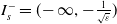 $I_s^- = (\!-\infty , -\frac {1}{\sqrt {\varepsilon }})$
and
$I_s^- = (\!-\infty , -\frac {1}{\sqrt {\varepsilon }})$
and $I_s^+ = (\frac {1}{\sqrt {\varepsilon }}, \infty )$
and a fast region
$I_s^+ = (\frac {1}{\sqrt {\varepsilon }}, \infty )$
and a fast region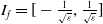 $I_f = [-\frac {1}{\sqrt {\varepsilon }}, \frac {1}{\sqrt {\varepsilon }}]$
. The boundaries of the fast region
$I_f = [-\frac {1}{\sqrt {\varepsilon }}, \frac {1}{\sqrt {\varepsilon }}]$
. The boundaries of the fast region $I_f$
are placed in the transition zone, satisfying
$I_f$
are placed in the transition zone, satisfying $|\xi | \gg 1$
and
$|\xi | \gg 1$
and $|x| \ll 1$
. In other words, the exact location of
$|x| \ll 1$
. In other words, the exact location of $\partial I_f$
is not critical [Reference Doelman, Gardner and Kaper12, Reference Doelman and Veerman16]. Indeed, the width of
$\partial I_f$
is not critical [Reference Doelman, Gardner and Kaper12, Reference Doelman and Veerman16]. Indeed, the width of $I_f$
should be chosen appropriately to ensure that
$I_f$
should be chosen appropriately to ensure that $v_h(\xi )$
is exponentially small everywhere outside
$v_h(\xi )$
is exponentially small everywhere outside $I_f$
, while
$I_f$
, while $u_h(\xi )$
remains approximately constant, to the leading order, within the fast region
$u_h(\xi )$
remains approximately constant, to the leading order, within the fast region $I_f$
.
$I_f$
.
Remark 2. For convenience, we denote by $\mathcal{W}^{u}(T_o)$
the collection of unstable fibres with base points on the curve
$\mathcal{W}^{u}(T_o)$
the collection of unstable fibres with base points on the curve $T_o$
and by
$T_o$
and by $\mathcal{W}^{s}(T_d)$
the collection of stable fibres with base points on the curve
$\mathcal{W}^{s}(T_d)$
the collection of stable fibres with base points on the curve $T_d$
. These sets intersect forming a
$T_d$
. These sets intersect forming a $2$
-dimensional manifold, denoted as
$2$
-dimensional manifold, denoted as $\mathcal{W}^{s}(T_d)\cap \mathcal{W}^{u}(T_o)$
. In the subsequent analysis, we will prove that
$\mathcal{W}^{s}(T_d)\cap \mathcal{W}^{u}(T_o)$
. In the subsequent analysis, we will prove that
 \begin{equation} \mathcal{W}^{s}(\mathcal{M}_{\varepsilon })\cap \mathcal{W}^{u}(\mathcal{M}_{\varepsilon })=\mathcal{W}^{s}(T_d)\cap \mathcal{W}^{u}(T_o). \end{equation}
Remark 3. In our setup, the heterogeneity region $ [-L, L]$
is defined in terms of the super-slow spatial variable
$ [-L, L]$
is defined in terms of the super-slow spatial variable $ \chi = \varepsilon x=\varepsilon ^2 \xi$
, as introduced in equation (1.2). Thus, in terms of the original spatial variable
$ \chi = \varepsilon x=\varepsilon ^2 \xi$
, as introduced in equation (1.2). Thus, in terms of the original spatial variable $ \xi$
, the corresponding heterogeneous region is rescaled to
$ \xi$
, the corresponding heterogeneous region is rescaled to $ \left [ -\frac {L}{\varepsilon ^2}, \frac {L}{\varepsilon ^2} \right ]$
, which becomes much wider as
$ \left [ -\frac {L}{\varepsilon ^2}, \frac {L}{\varepsilon ^2} \right ]$
, which becomes much wider as $ \varepsilon \to 0$
. On the other hand, the fast region is defined as
$ \varepsilon \to 0$
. On the other hand, the fast region is defined as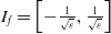 $ I_f = \left [ -\frac {1}{\sqrt {\varepsilon }}, \frac {1}{\sqrt {\varepsilon }} \right ]$
. Therefore, we have
$ I_f = \left [ -\frac {1}{\sqrt {\varepsilon }}, \frac {1}{\sqrt {\varepsilon }} \right ]$
. Therefore, we have
 \begin{equation*} \left [ -\frac {1}{\sqrt {\varepsilon }}, \frac {1}{\sqrt {\varepsilon }} \right ] \subset \left [ -\frac {L}{\varepsilon ^2}, \frac {L}{\varepsilon ^2} \right ]. \end{equation*}
In the fast system (2.2), the Hamiltonian $H(v,q;\;u)$
becomes a slowly varying function. Its derivative with respect to the fast time variable
$H(v,q;\;u)$
becomes a slowly varying function. Its derivative with respect to the fast time variable $\xi$
is given by
$\xi$
is given by
 \begin{equation} H_{\xi }(v,q;\;u)=\big (G(u,v,\varepsilon )-G(u,v,0)\big )q-\varepsilon p\int ^v_0 G_u( u,s,0)\,\textrm {d}s +\mathcal{O}(\varepsilon ^2). \end{equation}
The unperturbed homoclinic orbit $(u^{(0)},p^{(0)},v_{0}(\xi ),q_{0}(\xi ))$
is perturbed to a solution of the full fast system (2.2), denoted by
$(u^{(0)},p^{(0)},v_{0}(\xi ),q_{0}(\xi ))$
is perturbed to a solution of the full fast system (2.2), denoted by
 \begin{equation*}\gamma _{h}(\xi )=\left (u_h(\xi ),\,p_h(\xi ),\,v_h(\xi ),\,q_h(\xi )\right ),\end{equation*}
which is homoclinic to $\mathcal{M}_{\varepsilon }$
, provided that the Melnikov integral
$\mathcal{M}_{\varepsilon }$
, provided that the Melnikov integral
 \begin{equation} \begin{aligned} \triangle _{I_{f}}H(u,p) =& \int _{I_{f}} \big (G(u_{h}(\xi ),v_{h}(\xi ),\varepsilon )-G(u_{h}(\xi ),v_{h}(\xi ),0)\big )q_{h}(\xi )\,\textrm {d}\xi \\[5pt] & \quad -\varepsilon \int _{I_{f}} p_{h}(\xi ) \int ^{v_{h}(\xi )}_0 G_u( u_{h}(\xi ),s,0)\,\textrm {d}s \textrm {d} \xi +\mathcal{O}(\varepsilon ^2) \end{aligned} \end{equation}
has a simple zero. In that case, we have $\gamma _{h}(\xi )\subset \mathcal{W}^{s}(\mathcal{M}_\varepsilon )\cap \mathcal{W}^{u}(\mathcal{M}_\varepsilon )$
. The improper integral is well-defined because
$\gamma _{h}(\xi )\subset \mathcal{W}^{s}(\mathcal{M}_\varepsilon )\cap \mathcal{W}^{u}(\mathcal{M}_\varepsilon )$
. The improper integral is well-defined because $\gamma _{h}(\xi )$
converges exponentially to
$\gamma _{h}(\xi )$
converges exponentially to $(0,0,0,0)$
as
$(0,0,0,0)$
as $\xi \rightarrow \pm \infty$
.
$\xi \rightarrow \pm \infty$
.
To leading order,
 \begin{equation} \begin{aligned} \triangle _{I_{f}}H(u^{(0)},p^{(0)}) =& \int _{I_{f}} \big (G(u^{(0)},v_{0}(\xi ),\varepsilon )-G(u^{(0)},v_{0}(\xi ),0)\big )q_{0}(\xi )\,\textrm {d}\xi \\[5pt] & \quad \quad \quad \quad -\varepsilon \int _{I_{f}} p^{(0)} \int ^{v_{0}(\xi )}_0 G_u( u^{(0)},s,0)\,\textrm {d}s\textrm {d}\xi . \end{aligned} \end{equation}
Since $v_{ 0}(\xi )$
is even and
$v_{ 0}(\xi )$
is even and $q_{0}(\xi )$
is odd, so
$q_{0}(\xi )$
is odd, so $\big (G(u^{(0)},v_{0}(\xi ),\varepsilon )-G(u^{(0)},v_{0}(\xi ),0)\big )$
and
$\big (G(u^{(0)},v_{0}(\xi ),\varepsilon )-G(u^{(0)},v_{0}(\xi ),0)\big )$
and $\int ^{v_{0}(\xi )}_0 G_u( u^{(0)},s,0)\,\textrm { d}s$
are even functions. Note that
$\int ^{v_{0}(\xi )}_0 G_u( u^{(0)},s,0)\,\textrm { d}s$
are even functions. Note that $u^{(0)}$
is assumed to be positive; it then follows from (A1) that
$u^{(0)}$
is assumed to be positive; it then follows from (A1) that $G_u( u^{(0)},v,0)$
is also positive. Consequently, solving
$G_u( u^{(0)},v,0)$
is also positive. Consequently, solving $\triangle _{I_{f}}H(u^{(0)},p^{(0)})=0$
gives
$\triangle _{I_{f}}H(u^{(0)},p^{(0)})=0$
gives $p^{(0)}=0$
.
$p^{(0)}=0$
.
To compute the correction, we expand $(u_{h}(\xi ), p_{h}(\xi ), v_{h}(\xi ), q_{h}(\xi ))$
in the power of
$(u_{h}(\xi ), p_{h}(\xi ), v_{h}(\xi ), q_{h}(\xi ))$
in the power of $\varepsilon$
, namely,
$\varepsilon$
, namely,
 \begin{align} \begin{aligned} u_{h}(\xi )&=u^{(0)}+ \varepsilon u_{1}(\xi )+ \textrm {h.o.t.}, \\[5pt] p_{h}(\xi )&= \varepsilon p_{1}(\xi )+ \textrm {h.o.t.}, \\[5pt] v_{h}(\xi )&=v_{0}(\xi )+\textrm {h.o.t.},\\[5pt] q_{h}(\xi )&=q_{0}(\xi )+\textrm {h.o.t.}, \end{aligned} \end{align}
where the initial conditions are $u_{h}(0)=u^{(0)}$
and
$u_{h}(0)=u^{(0)}$
and $u_{j}(0)=0$
for all
$u_{j}(0)=0$
for all $j\geq 1$
. Substituting (2.9) into (2.2) gives
$j\geq 1$
. Substituting (2.9) into (2.2) gives
 \begin{equation*} u_{1}(\xi )\equiv 0,\,\,\, p_{1}(\xi )=\int _{0}^{\xi }F\big (u^{(0)},v_0(\omega )\big )\,\textrm {d}\omega + p_{1}(0). \end{equation*}
Note that the integral term in $p_{1}(\xi )$
is an odd function since
$p_{1}(\xi )$
is an odd function since $v_{ 0}(\xi )$
is an even function; thus, (2.7) becomes
$v_{ 0}(\xi )$
is an even function; thus, (2.7) becomes
 \begin{equation} \begin{aligned} \int _{I_{f}}H_{\xi }\,\textrm {d}\xi =&\int ^{+\infty }_{-\infty } \big (G(u^{(0)},v_{0}(\xi ),\varepsilon )-G(u^{(0)},v_{0}(\xi ),0)\big )q_{0}(\xi )\,\textrm {d}\xi \\[5pt] &\quad -\varepsilon \int ^{+\infty }_{-\infty }(p^{(0)}+ \varepsilon p_{1}(\xi ))\int ^{v_{0}(\xi )}_0 G_u( u^{(0)},s,0)\,\textrm { d}s \textrm {d}\xi + \textrm {h.o.t.}\\[5pt] =&-2\varepsilon (p^{(0)}+\varepsilon p_1(0))\int ^{+\infty }_{0} \int ^{v_{0}(\xi )}_0 G_u( u^{(0)},s,0)\,\textrm {d}s \textrm { d}\xi +\textrm {h.o.t.} \end{aligned} \end{equation}
Since $u_0$
is positive, the integral in (2.10) is also positive by the assumption (A1). Therefore, we conclude that the condition for vanishing Melnikov integral up to
$u_0$
is positive, the integral in (2.10) is also positive by the assumption (A1). Therefore, we conclude that the condition for vanishing Melnikov integral up to $\mathcal{O}(\varepsilon ^2)$
is
$\mathcal{O}(\varepsilon ^2)$
is
 \begin{equation*}p^{(0)}=0,\,\,\,\qquad \,\,\, p_1(0)=0.\end{equation*}
Remark 4. For any orbit
 \begin{equation*} \gamma _{h}(\xi )=(u_{h}(\xi ), p_{h}(\xi ), v_{h}(\xi ), q_{h}(\xi )) \subset \mathcal{W}^{s}(\mathcal{M}_\varepsilon )\cap \mathcal{W}^{u}(\mathcal{M}_\varepsilon ),\end{equation*}
it follows from the reversibility symmetry that
 \begin{align} u_{h}(\xi )=u_{h}(\!-\xi ),\quad \quad v_{h}(\xi )=v_{h}(\!-\xi ). \end{align}
Therefore, $\xi = 0$
must be an extremum (specifically, a local maximum) of both
$\xi = 0$
must be an extremum (specifically, a local maximum) of both $u_{h}(\xi )$
and
$u_{h}(\xi )$
and $v_{h}(\xi )$
. By Fermat’s Lemma, this yields
$v_{h}(\xi )$
. By Fermat’s Lemma, this yields $p_{h}(0)=0$
and
$p_{h}(0)=0$
and $q_{h}(0)=0$
.
$q_{h}(0)=0$
.
Define the Take-off curve $T_{o}$
and the Touch-down curve
$T_{o}$
and the Touch-down curve $T_{d}$
on
$T_{d}$
on $\mathcal{M_{\varepsilon }}$
by
$\mathcal{M_{\varepsilon }}$
by
 \begin{equation} T_{o/d}=\left \{(u,p,v,q)\left |\,u=u_h\left (\mp \frac {1}{\sqrt {\varepsilon }}\right ),\,p=p_h\left (\mp \frac {1}{\sqrt {\varepsilon }}\right ),\right .v=q=0\right \} \end{equation}
with $p=\frac {1}{\varepsilon }\frac {d\,u}{d\,\xi }$
. By (2.2), we have
$p=\frac {1}{\varepsilon }\frac {d\,u}{d\,\xi }$
. By (2.2), we have
 \begin{equation} \begin{aligned} \Delta u=\int _{I_{f}}u_{\xi }\,\text{d}\xi =&\int _{I_{f}}\varepsilon ^2p_{1}(\xi )\,\text{d}\xi =\mathcal{O}(\varepsilon ^{3/2}),\\[5pt] \Delta p= \int _{I_{f}}p_{\xi }\,\text{d}\xi =&\int _{I_{f}}\varepsilon F(u,v(\xi )) + \mathcal{O}(\varepsilon ^{3})\,\text{d}\xi \\[5pt] =&\,2\varepsilon \int ^{0}_{-\infty } F(u,v_0(\xi )) \,\text{ d}\xi +\mathcal{O}(\varepsilon ^{2}), \end{aligned} \end{equation}
where we have used the facts that $u_{\xi }=\varepsilon p$
and
$u_{\xi }=\varepsilon p$
and $p=\mathcal{O}(\varepsilon )$
during
$p=\mathcal{O}(\varepsilon )$
during $I_f$
in the first equation, and
$I_f$
in the first equation, and $v_0(\xi )$
is an even function with respect to
$v_0(\xi )$
is an even function with respect to $\xi$
in the second equation. So, to leading order, the explicit representations of the Take-off curve
$\xi$
in the second equation. So, to leading order, the explicit representations of the Take-off curve $T_{o}$
and the Touch-down curve
$T_{o}$
and the Touch-down curve $T_{d}$
on
$T_{d}$
on $\mathcal{M_{\varepsilon }}$
are, respectively
$\mathcal{M_{\varepsilon }}$
are, respectively
 \begin{equation} T_{o,d}(u)=\big \{(u,p,0,0)\in \mathcal{M_{\varepsilon }}\,|\,p= \mathcal{T}_{\mp }(u)+\mathcal{O}(\varepsilon ^{2}),\,u\gt 0\,\big \}, \end{equation}
where $\mathcal{T}_{\mp }(u)=\mp \varepsilon \int ^{0}_{-\infty } F(u,v_0(\xi ))\text{ d}\xi$
and
$\mathcal{T}_{\mp }(u)=\mp \varepsilon \int ^{0}_{-\infty } F(u,v_0(\xi ))\text{ d}\xi$
and $p=\frac {1}{\varepsilon }\frac {du}{d\xi }$
.
$p=\frac {1}{\varepsilon }\frac {du}{d\xi }$
.
Remark 5. The homoclinic solution $(v_{0}(\xi;\;u), q_{0}(\xi;\;u))$
of system (2.3) provides the leading order solution of (2.2), given by
$(v_{0}(\xi;\;u), q_{0}(\xi;\;u))$
of system (2.3) provides the leading order solution of (2.2), given by
 \begin{equation} \phi _h(\xi )\;:\!=\;\left (u, \varepsilon \int ^{\xi }_{0} F(u,v_0(x;\;u))\,\textrm {d}x,v_{0}(\xi;\;u), q_{0}(\xi;\;u)\right ), \end{equation}
which is homoclinic to $\mathcal{M}_{\varepsilon }$
. Moreover, its asymptotic limits
$\mathcal{M}_{\varepsilon }$
. Moreover, its asymptotic limits $\lim _{\xi \to \pm \infty } \phi _h(\xi )$
correspond precisely to the Touch-down and Take-off curves.
$\lim _{\xi \to \pm \infty } \phi _h(\xi )$
correspond precisely to the Touch-down and Take-off curves.
2.2. Slow dynamics on the slow manifold
A singular homoclinic orbit is constructed by concatenating trajectories of the fast and slow limiting systems. Though this singular homoclinic orbit is not an exact solution to system (2.2), GSPT ensures that a true homoclinic orbit exists within a small neighbourhood of this singular trajectory. In the previous subsection, the trajectories of the fast limiting system had been derived. In this section, we focus on the slow dynamics on the slow manifold and match them with the fast segments to complete the full orbit.
On the slow manifold
 \begin{equation} \mathcal{M}_{\varepsilon }=\{(u, p, v, q) | v=q=0,\,u\gt 0\}, \end{equation}
the dynamics of system (2.2) are governed by
 \begin{equation} u_{\xi \xi }=\varepsilon ^{4}\frac {\partial }{\partial u}W(u,\chi ). \end{equation}
In the super-slow coordinate $\chi =\varepsilon ^2 \xi$
, the slow limiting system can be transformed into
$\chi =\varepsilon ^2 \xi$
, the slow limiting system can be transformed into
 \begin{equation} \left \{ {\begin{array}{l} u_{\chi }=p,\\[10pt] p_{\chi }=\dfrac {\partial }{\partial u}W(u,\chi ),\\[5pt] \end{array}} \right . \end{equation}
which is a non-autonomous Hamiltonian system with
 \begin{equation} H_s(u,p)=\frac {1}{2}p^2-W(u,\chi ). \end{equation}
It follows from (A3) that system (2.18) admits a saddle $(0,0)$
. The slow trajectories can be constructed via the phase plane analysis on two autonomous Hamiltonian systems,
$(0,0)$
. The slow trajectories can be constructed via the phase plane analysis on two autonomous Hamiltonian systems,
 \begin{equation} \left \{ {\begin{array}{l} u_{\chi }=p,\\[5pt] p_{\chi }=W^{\prime }_i(u), \end{array}} \right .\qquad i=1,2, \end{equation}
where $W^{\prime }_i(u)$
are the potentials outside and inside the heterogeneous region, respectively. Appropriate boundary conditions must be imposed to ensure that the matching between the trajectories and their derivatives at the endpoints of each region can be performed. These trajectories decay exponentially to
$W^{\prime }_i(u)$
are the potentials outside and inside the heterogeneous region, respectively. Appropriate boundary conditions must be imposed to ensure that the matching between the trajectories and their derivatives at the endpoints of each region can be performed. These trajectories decay exponentially to $(0,0)$
as
$(0,0)$
as $\chi \rightarrow \pm \infty$
. In this manner, the solutions to system (2.18) are
$\chi \rightarrow \pm \infty$
. In this manner, the solutions to system (2.18) are $\textrm{C}^1$
-smooth.
$\textrm{C}^1$
-smooth.
In the following, we will demonstrate that the value of the Hamiltonian $h$
inside the heterogeneity with the length
$h$
inside the heterogeneity with the length $2L$
serves as an important parameter to characterise the pinned pulses. A pinned pulse is generally determined by four points in the phase plane, namely:
$2L$
serves as an important parameter to characterise the pinned pulses. A pinned pulse is generally determined by four points in the phase plane, namely:
-
• The points where the pinned pulse enters and exits the heterogeneous region, respectively, denoted by
$(u_{in}, p_{in})$
and
$(u_{out}, p_{out})$
. -
• The points where the pinned pulse enters and exits the fast field, respectively, denoted by
$(u_0, p_0)$
and
$(u_d, p_d)$
.


Since system (2.2) is symmetric under $\chi \rightarrow -\chi$
, we have
$\chi \rightarrow -\chi$
, we have
 \begin{align*} \begin{aligned} u_{in} &= u_{out}, \qquad \qquad p_{in} = -p_{out},\\[5pt] u_{0}\, &= u_{d},\qquad \qquad \,\,\, p_{0}\, = -p_{d}. \end{aligned} \end{align*}
Therefore, only $(u_{in}, p_{in})$
and
$(u_{in}, p_{in})$
and $(u_0, p_0)$
need to be determined. More precisely,
$(u_0, p_0)$
need to be determined. More precisely, $(u_{in}, p_{in})$
is the intersection between the unstable manifold of the saddle
$(u_{in}, p_{in})$
is the intersection between the unstable manifold of the saddle $(0, 0)$
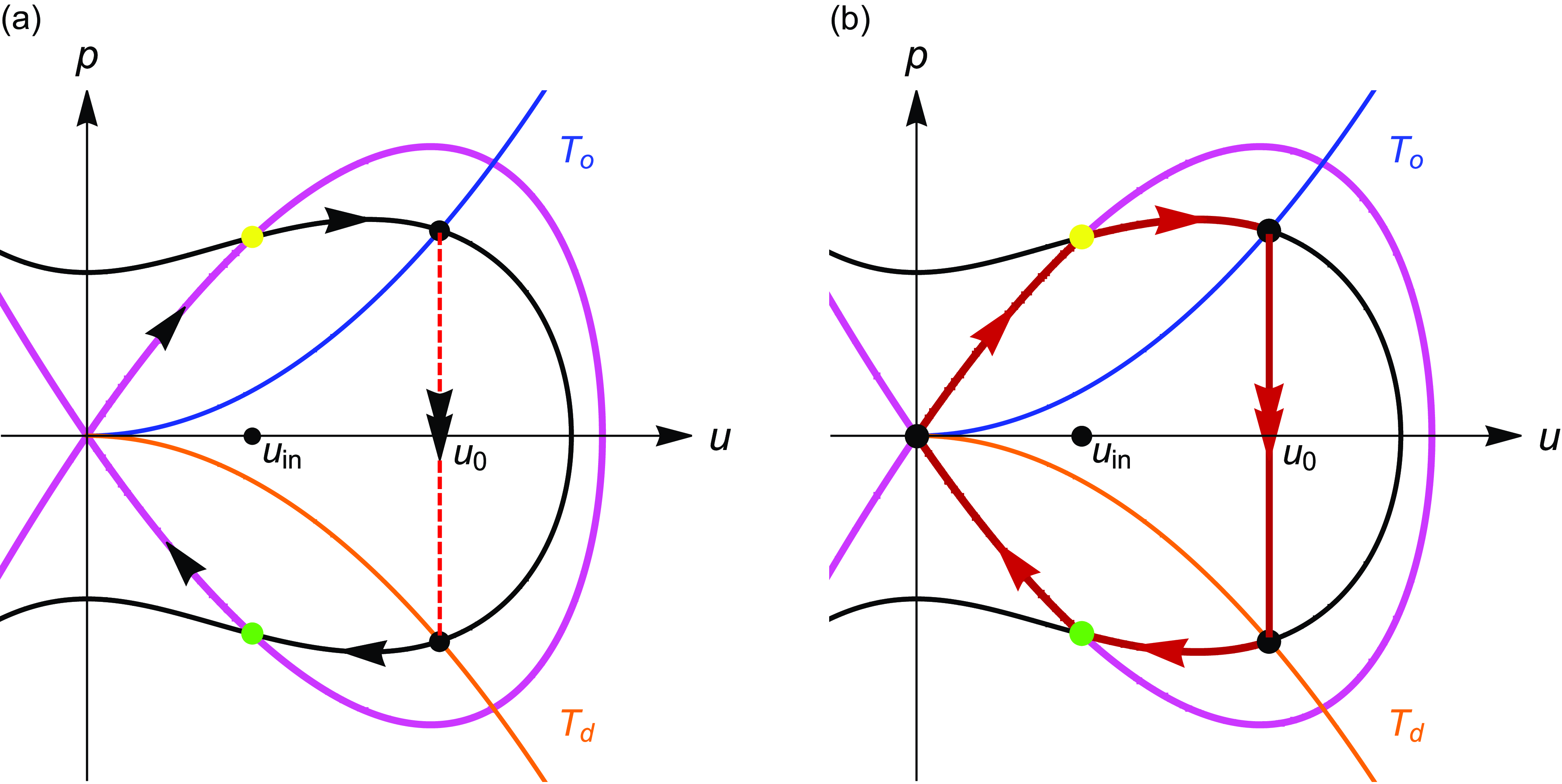
outside the heterogeneity (the purple solid curve in Figure 2) and the level set
$(0, 0)$
outside the heterogeneity (the purple solid curve in Figure 2) and the level set $H_s(u, p) = h$
within the heterogeneous region (the black curve). They satisfy
$H_s(u, p) = h$
within the heterogeneous region (the black curve). They satisfy
 \begin{equation} \begin{aligned} 0&=p_{in}^2-2W_1(u_{in}),\\[5pt] 2h&=p_{in}^2-2W_2(u_{in}), \end{aligned} \end{equation}
where
 \begin{equation*} W^{\prime }_1(u_{in})-W^{\prime }_2(u_{in})\neq 0 \end{equation*}
is required to ensure that the intersection between such two slow trajectories is transverse, and $h$
represents the Hamiltonian value within the heterogeneity. By solving system (2.21), we can obtain
$h$
represents the Hamiltonian value within the heterogeneity. By solving system (2.21), we can obtain $(u_{in}, p_{in}) = (u_{in}(h), p_{in}(h))$
, where
$(u_{in}, p_{in}) = (u_{in}(h), p_{in}(h))$
, where $h$
acts as a free parameter.
$h$
acts as a free parameter.
Singular homoclinic orbit of system (2.2) with $1$
fast and
$1$
fast and $4$
slow segments. Left panel: two slow segments outside the heterogeneity are marked by the solid purple curves, indicating the stable and unstable manifolds of the saddle
$4$
slow segments. Left panel: two slow segments outside the heterogeneity are marked by the solid purple curves, indicating the stable and unstable manifolds of the saddle $(0, 0)$
; two slow segments inside the heterogeneity (the black curves), representing the orbits defined by
$(0, 0)$
; two slow segments inside the heterogeneity (the black curves), representing the orbits defined by $H_s(u,p)=h$
; and a fast segment is indicated by the red dashing line. In the figure, the yellow dot represents
$H_s(u,p)=h$
; and a fast segment is indicated by the red dashing line. In the figure, the yellow dot represents $(u_{in}, p_{in})$
, and the green one stands for
$(u_{in}, p_{in})$
, and the green one stands for $(u_{out}, p_{out})$
. Right panel: the thick red curve indicates the whole singular homoclinic orbit.
$(u_{out}, p_{out})$
. Right panel: the thick red curve indicates the whole singular homoclinic orbit.
Remark 6. Let $u=u_{in,k}\gt 0$
,
$u=u_{in,k}\gt 0$
, $k=1, 2, \cdots , K$
, be the
$k=1, 2, \cdots , K$
, be the $K$
non-degenerate solutions obtained from (2.21), then there exist
$K$
non-degenerate solutions obtained from (2.21), then there exist $2K$
distinct points
$2K$
distinct points $(u_{in,k}, p^{\pm }_{in,k})$
. These points play a key role in constructing the transversely intersecting homoclinic orbits.
$(u_{in,k}, p^{\pm }_{in,k})$
. These points play a key role in constructing the transversely intersecting homoclinic orbits.
Based on the curves $T_{o,d}$
on
$T_{o,d}$
on $\mathcal{M}_\varepsilon$
defined in (2.14), a homoclinic orbit
$\mathcal{M}_\varepsilon$
defined in (2.14), a homoclinic orbit $\phi _h$
of the limiting fast system (2.3) can be connected with the slow orbits on the slow manifold
$\phi _h$
of the limiting fast system (2.3) can be connected with the slow orbits on the slow manifold $\mathcal{M}_\varepsilon$
to construct a singular homoclinic orbit. To guarantee that this singular orbit persists under small perturbations, it is essential that the Take-off curve
$\mathcal{M}_\varepsilon$
to construct a singular homoclinic orbit. To guarantee that this singular orbit persists under small perturbations, it is essential that the Take-off curve $T_o$
intersects transversely with the orbit of the 2nd system (2.20). The corresponding intersection point
$T_o$
intersects transversely with the orbit of the 2nd system (2.20). The corresponding intersection point $(u_0, p_0)$
is governed by
$(u_0, p_0)$
is governed by
 \begin{equation} \begin{aligned} p_0 & = \mathcal{T}_-(u_0),\\[5pt] 2h & = p_{0}^2 - 2W_2(u_{0}), \end{aligned} \end{equation}
where it is also required that
 \begin{equation*} \mathcal{T}_-(u_0)\mathcal{T}_-^{\prime }(u_0) - W^{\prime }_2(u_{0})\neq 0 \end{equation*}
such that the matching is transverse.
If both equations (2.21) and (2.22) admit non-degenerate solutions $(u_{in}(h), p_{in}(h))$
and
$(u_{in}(h), p_{in}(h))$
and $(u_0(h), p_0(h))$
, this implies that
$(u_0(h), p_0(h))$
, this implies that
-
• The outer and inner slow trajectories intersect transversely at the position of heterogeneity.
-
• The slow trajectory intersects with the fast jump trajectory transversely.
However, the Hamiltonian value $h$
remains undetermined now. To determine it, we impose the condition that the ‘time’ for the slow trajectory to evolve from
$h$
remains undetermined now. To determine it, we impose the condition that the ‘time’ for the slow trajectory to evolve from $(u_{in}(h), p_{in}(h))$
to
$(u_{in}(h), p_{in}(h))$
to $(u_0(h), p_0(h))$
is exactly
$(u_0(h), p_0(h))$
is exactly $L$
(the half-width of the heterogeneous region). Once this condition is satisfied, we get a singular homoclinic orbit from the saddle to itself with transversality. By GSPT, there are true homoclinic orbits in a small neighbourhood of this singular configuration.
$L$
(the half-width of the heterogeneous region). Once this condition is satisfied, we get a singular homoclinic orbit from the saddle to itself with transversality. By GSPT, there are true homoclinic orbits in a small neighbourhood of this singular configuration.
Remark 7. The relative positions of $(u_{in}, p_{in})$
and
$(u_{in}, p_{in})$
and $(u_{0}, p_{0})$
, respectively, determined by (2.21) and (2.22) are crucial for constructing the different types of singular homoclinic orbits. It is worth noting that the orbits in the 2nd system possessing through ‘turning points’ are particularly important for constructing pinned pulses with certain dynamical properties.
$(u_{0}, p_{0})$
, respectively, determined by (2.21) and (2.22) are crucial for constructing the different types of singular homoclinic orbits. It is worth noting that the orbits in the 2nd system possessing through ‘turning points’ are particularly important for constructing pinned pulses with certain dynamical properties.


3. Pinned pulses in a non-autonomous Gierer–Meinhardt equation
Consider
 \begin{equation} \left \{ {\begin{array}{l} \varepsilon ^{2}U_{t}=\quad U_{xx}-\varepsilon ^{2}(f(\chi ) U-g(\chi ) U^d)+\sigma V^{2},\\[10pt] \,\,\,V_{t}=\varepsilon ^{2}V_{xx}-V+\dfrac {V^{2}}{U}, \end{array}} \right . \end{equation}
where $\sigma \neq 0$
,
$\sigma \neq 0$
, $d\gt 1$
and
$d\gt 1$
and
 \begin{equation} f(\chi )= \left \{ {\begin{array}{l} \alpha _1, \quad \quad |\chi |\gt L,\\[5pt] \alpha _2, \quad \quad |\chi |\lt L, \end{array}}\quad \quad \,g(\chi )= \left \{\begin{array}{l} {\gamma _1, \quad \quad |\chi |\gt L},\\[5pt] {\gamma _2, \quad \quad |\chi |\lt L}. \end{array} \right . \right . \end{equation}
The associated fast limiting system is
 \begin{equation} \left \{ {\begin{array}{l} v^\prime =q,\\[10pt] q^{\prime }=v-\dfrac {v^{2}}{u}, \\[5pt] \end{array}} \right . \end{equation}
which admits a saddle $(0,0)$
and a homoclinic orbit described by
$(0,0)$
and a homoclinic orbit described by
 \begin{align} \begin{aligned} v_{0}(\xi ,u)&=\frac {3u}{2} \textrm {sech}^{2}\left (\frac {\xi }{2}\right ),\quad \quad \quad \quad \,\\[5pt] q_{0}(\xi ,u)&= -\frac {3u}{2}\textrm {sech}^{2}\left (\frac {\xi }{2}\right )\tanh \left (\frac {\xi }{2}\right ). \end{aligned} \end{align}
The explicit homoclinic orbit solution (3.4) of (3.3) is well-known (see, e.g. [Reference Sewalt and Doelman31, Reference Veerman and Doelman37]). By direct calculations, the Take-off and Touch-down curves are, respectively
 \begin{equation} T_{o/d}(u)=\left \{(u,p,0,0)\in \mathcal{M_{\varepsilon }}\,|\,p= \pm 3\varepsilon \sigma u^2+\mathcal{O}(\varepsilon ^2),\,u\gt 0\right \}. \end{equation}
Note that for $\sigma \gt 0$
, the Take-off curve lies in the first quadrant of the
$\sigma \gt 0$
, the Take-off curve lies in the first quadrant of the $(u, p)$
plane, while for
$(u, p)$
plane, while for $\sigma \lt 0$
, it lies in the fourth quadrant. Thus, changing the sign of
$\sigma \lt 0$
, it lies in the fourth quadrant. Thus, changing the sign of $\sigma$
reverses the direction of the fast jump (see Figures 3 and 4).
$\sigma$
reverses the direction of the fast jump (see Figures 3 and 4).
The limiting slow system corresponding to (2.18) becomes
 \begin{equation} \left \{ {\begin{array}{l} u_{\chi }=p,\\[5pt] p_{\chi }=f(\chi ) u -g(\chi ) u^d,\\[5pt] \end{array}} \right . \end{equation}
which has a saddle at $(0,0)$
when
$(0,0)$
when $\alpha _1\gt 0$
. This is a piecewise Hamiltonian system with
$\alpha _1\gt 0$
. This is a piecewise Hamiltonian system with
 \begin{equation} H_s(u,p)=\frac {1}{2}p^2-\left (\frac {f(\chi ) }{2} u^2-\frac {g(\chi ) }{d+1}u^{d+1}\right ). \end{equation}
The matching condition for the entry point $(u_{in}, p_{in})$
is given by
$(u_{in}, p_{in})$
is given by
 \begin{equation} \begin{aligned} 0&=p_{in}^2-\left (\alpha _1 u_{in}^2-\frac {2\gamma _1 }{d+1}u_{in}^{d+1}\right ),\\[5pt] 2h&=p_{in}^2-\left (\alpha _2 u_{in}^2-\frac {2\gamma _2 }{d+1}u_{in}^{d+1}\right ),\\[5pt] 0&\neq (\alpha _1-\alpha _2) u_{in}-(\gamma _1-\gamma _2) u_{in}^{d}, \end{aligned} \end{equation}
where $h$
represents the Hamiltonian within the heterogeneous region. Similarly, the matching condition between the slow and fast orbits can be given by
$h$
represents the Hamiltonian within the heterogeneous region. Similarly, the matching condition between the slow and fast orbits can be given by
 \begin{equation} \begin{aligned} p_0&=3\sigma u^2_0,\\[5pt] 2h&=p_{0}^2-\left (\alpha _2 u_{0}^2-\frac {2\gamma _2 }{d+1}u_0^{d+1}\right ),\\[5pt] 0&\neq 18\sigma ^2 u^3_0-\Big (\alpha _2 u_{0}-\gamma _2 u_{0}^{d}\Big ). \end{aligned} \end{equation}
In what follows, we consider two distinct cases.
3.1. Case 1:
$g(\chi )\equiv 0$
.

Through this simplest case, we can illustrate the key idea of the geometric approach clearly.
Under $g(\chi )\equiv 0$
, the matching conditions in equation (3.8) reduce to
$g(\chi )\equiv 0$
, the matching conditions in equation (3.8) reduce to
 \begin{equation} \begin{aligned} 0&=p_{in}^2-\alpha _1 u_{in}^2,\\[5pt] 2h&=p_{in}^2-\alpha _2 u_{in}^2. \end{aligned} \end{equation}
Solving these two equations yields the explicit expressions for $u_{in}$
and
$u_{in}$
and $p_{in}$
in terms of
$p_{in}$
in terms of $h$
, namely,
$h$
, namely,
 \begin{equation} u_{in}(h)=\sqrt {\frac {2h}{\alpha _1-\alpha _2}},\qquad \quad p_{in}(h)=\sqrt {\frac {2h \alpha _1}{\alpha _1-\alpha _2}}, \end{equation}
where $\textrm {sign}(h)=\textrm {sign}(\alpha _1-\alpha _2)$
, which ensures that
$\textrm {sign}(h)=\textrm {sign}(\alpha _1-\alpha _2)$
, which ensures that $u_{in}(h),\, p_{in}(h)\gt 0$
. By direct calculations, when
$u_{in}(h),\, p_{in}(h)\gt 0$
. By direct calculations, when $\sigma \gt 0$
and
$\sigma \gt 0$
and $\textrm {sign}(h)=\textrm {sign}(\alpha _1-\alpha _2)$
, (3.9) can be simplified as
$\textrm {sign}(h)=\textrm {sign}(\alpha _1-\alpha _2)$
, (3.9) can be simplified as
 \begin{align} \begin{aligned} u_{0}(h)=u^\pm _{0}(h) =\frac {\left (\alpha _2\pm \sqrt {\alpha _2^2+72\sigma ^2h}\,\right )^\frac {1}{2}}{3\sqrt {2}\sigma }, \end{aligned} \end{align}
where we only consider $u_0(h)\in \mathbb{R}_+$
(
$u_0(h)\in \mathbb{R}_+$
( $u_{0}(h)=u^-_{0}(h)$
is valid only when
$u_{0}(h)=u^-_{0}(h)$
is valid only when $\alpha _1\lt \alpha _2$
, which is discarded). Thus, the condition
$\alpha _1\lt \alpha _2$
, which is discarded). Thus, the condition $u_0(h)\gt u_{in}(h)$
is equivalent to
$u_0(h)\gt u_{in}(h)$
is equivalent to
 \begin{equation} \frac {\left (\alpha _2\pm \sqrt {\alpha _2^2-72\sigma ^2h}\,\right )^\frac {1}{2}}{3\sqrt {2}\sigma } \gt \sqrt {\frac {2h}{\alpha _1-\alpha _2}}. \end{equation}
Within the heterogeneous region, the slow orbit satisfies
 \begin{equation*}2h=p^2-\alpha _2 u^2\end{equation*}
with $p=u_{\chi }$
. Therefore, the relationship between the length
$p=u_{\chi }$
. Therefore, the relationship between the length $L$
and the Hamiltonian
$L$
and the Hamiltonian $h$
is
$h$
is
 \begin{equation} \begin{aligned} L&=\int ^0_{-L} \textrm{d}x=\int ^{u_0(h)}_{u_{in(h)}}\frac {\textrm{d}u}{p} =\int ^{u_0(h)}_{u_{in(h)}}\frac {\textrm{d}u}{\sqrt {2h+\alpha _2 u^2}}=I(u_0(h))-I(u_{in}(h)), \end{aligned} \end{equation}
where
 \begin{equation} I(u)= \begin{cases} \dfrac {1}{\sqrt {\alpha _2}} \log \, (2 \sqrt {\alpha _2 (2h+\alpha _2 u^2)}+2\alpha _2 u ), \quad \quad \quad & [\alpha _2 u\gt \sqrt {-\Delta },\, \quad \Delta \lt 0],\\[10pt] \dfrac {1}{\sqrt {\alpha _2}} \log \, ( \sqrt {\alpha _2 (2h+\alpha _2 u^2)}-2\alpha _2 u ), \quad & [2\alpha _2 u\lt -\sqrt {-\Delta }, \quad \Delta \lt 0],\\[10pt] \dfrac {1}{\sqrt {\alpha _2}} \operatorname {arcsinh}\left (\dfrac { \alpha _2 u}{\sqrt {\Delta }}\right ), \quad &[ \Delta \gt 0], \\[10pt] \dfrac {1}{\sqrt {\alpha _2}} \log \, (2\alpha _2 u), \quad &[\Delta =0], \end{cases} \end{equation}
and $\Delta =\alpha _2h$
. By combining (3.11), (3.12) and (3.14), the value of
$\Delta =\alpha _2h$
. By combining (3.11), (3.12) and (3.14), the value of $h$
can be implicitly determined. This determines the exact slow orbit used in the construction of the pinned pulse solution.
$h$
can be implicitly determined. This determines the exact slow orbit used in the construction of the pinned pulse solution.
The unstable and stable manifolds of the saddle $(0,0)$
are given by
$(0,0)$
are given by
 \begin{equation} u_{h,\mp }(\chi )=e^{\pm \sqrt {\alpha _1}\,(\chi \mp x_*)}, \end{equation}
where $x_*\gt 0$
is introduced such that
$x_*\gt 0$
is introduced such that $u_{h,-}(\!-L )=u_{in}$
. By the reversible symmetry, it follows that
$u_{h,-}(\!-L )=u_{in}$
. By the reversible symmetry, it follows that $u_{h,+}(L )=u_{out}$
. Within the heterogeneous region (
$u_{h,+}(L )=u_{out}$
. Within the heterogeneous region ( $|x|\lt L$
), the expression of the orbit is given explicitly by
$|x|\lt L$
), the expression of the orbit is given explicitly by
 \begin{equation} u_{i,\mp }(\chi )=A_{1,2} e^{-\sqrt {\alpha _2}\,\chi }+B_{1,2}e^{\sqrt {\alpha _2}\,\chi }, \end{equation}
where the constants $A_{1,2}$
and
$A_{1,2}$
and $B_{1,2}$
are determined to ensure that
$B_{1,2}$
are determined to ensure that $u_{p,0}(\chi )$
is continuously differentiable at
$u_{p,0}(\chi )$
is continuously differentiable at $\chi =\pm L$
. Thus, the composite solution can be defined by
$\chi =\pm L$
. Thus, the composite solution can be defined by
 \begin{equation} u_{p,0}(\chi ) = \begin{cases} u_{h,-}(\chi ) \,,\,\,\,\,\,\,\,\,\,\,\, \quad &\chi \, \in \,(\!-\infty ,-L), \\[5pt] u_{i,-}(\chi )\,, &\chi \, \in (\!-L,0),\quad \quad \\[5pt] u_{i,+}(\chi )\,, \quad &\chi \in \,(\,0,\,L\,),\quad \,\quad \,\\[5pt] u_{h,+}(\chi )\,,\,\,\,\,\,\,\,\,\,\,\,\,\,\,\,\,\,\,\,\,\,\, &\chi \,\in \,(L,+\infty ). \end{cases} \end{equation}
Hence, the smooth matching condition at $\chi =\pm L$
is given by
$\chi =\pm L$
is given by
 \begin{equation} \begin{pmatrix} e^{\sqrt {\alpha _2}\,L} & e^{-\sqrt {\alpha _2}\,L} & 0 & 0\\[5pt] -\sqrt {\alpha _2} e^{\sqrt {\alpha _2}\,L} &\sqrt {\alpha _2} e^{-\sqrt {\alpha _2}\,L} &0 &0\\[5pt] 0 & 0 & e^{-\sqrt {\alpha _2}\,L} & e^{\sqrt {\alpha _2}\,L}\\[5pt] 0 &0 &-\sqrt {\alpha _2} e^{-\sqrt {\alpha _2}\,L} &\sqrt {\alpha _2} e^{\sqrt {\alpha _2}\,L}\\[5pt] \end{pmatrix} \begin{pmatrix} A_{1}\\[5pt] B_{1}\\[5pt] A_{2}\\[5pt] B_{2} \end{pmatrix} =\begin{pmatrix} u_{in}\\[5pt] p_{in}\\[5pt] u_{out}\\[5pt] p_{out} \end{pmatrix}. \end{equation}
Solving (3.19) directly yields
 \begin{equation} \begin{aligned} A_{1}&=B_{2}=\frac {(\sqrt {\alpha _2} \,u_{in}-p_{in})e^{-\sqrt {\alpha _2}L}}{2\sqrt {\alpha _2}} =\frac {\alpha _2-\sqrt {\alpha _1\alpha _2}}{2\alpha _2}\sqrt {\frac {2h }{\alpha _1-\alpha _2}}e^{-\sqrt {\alpha _2}L}, \\[5pt] B_{1}&=A_{2}=\frac {(\sqrt {\alpha _2} u_{in}+p_{in})e^{\sqrt {\alpha _2}L}}{2\sqrt {\alpha _2}} =\frac {\alpha _2+\sqrt {\alpha _1\alpha _2}}{2\alpha _2}\sqrt {\frac {2h }{\alpha _1-\alpha _2}}\,e^{\sqrt {\alpha _2}L}. \end{aligned} \end{equation}
Theorem 3.
Let $\varepsilon \gt 0$
be sufficiently small, and
$\varepsilon \gt 0$
be sufficiently small, and $\alpha _1$
,
$\alpha _1$
, $\alpha _2,\,\sigma ,\,L\gt 0$
be given. Assume that (3.13) admits a non-degenerate root
$\alpha _2,\,\sigma ,\,L\gt 0$
be given. Assume that (3.13) admits a non-degenerate root $h$
satisfying
$h$
satisfying $\textrm {sign}(h)=\textrm { sign}(\alpha _1-\alpha _2)$
and that (3.14) holds, then system (3.1) with
$\textrm {sign}(h)=\textrm { sign}(\alpha _1-\alpha _2)$
and that (3.14) holds, then system (3.1) with $g(\chi )\equiv 0$
admits a pinned pulse solution
$g(\chi )\equiv 0$
admits a pinned pulse solution $(u_{h}(\xi ), v_{h}(\xi ))$
with
$(u_{h}(\xi ), v_{h}(\xi ))$
with
 \begin{equation} |v_{h}(\xi )-v_{0}(\xi;\;u_0(h_0))|,\,\,|u_{h}(\xi )-u_0(h_0)|=\mathcal{O}(\varepsilon ), \end{equation}
for $\xi \in I_f$
, where
$\xi \in I_f$
, where $v_{0}(\xi;\;u_0(h))$
and
$v_{0}(\xi;\;u_0(h))$
and $u_0(h)$
are given by (3.4) and (3.12), respectively. For
$u_0(h)$
are given by (3.4) and (3.12), respectively. For $\xi \in I_s^\pm$
, we have
$\xi \in I_s^\pm$
, we have
 \begin{equation} |v_{h}(\xi )|,\,\,|u_{h}(\chi )-u_{p,0}(\chi )|=\mathcal{O}(\varepsilon ), \end{equation}
where $u_{p,0}(\chi )$
is defined in (3.18).
$u_{p,0}(\chi )$
is defined in (3.18).
3.2.
Case 2:
$g(\chi )\neq 0$
.

In the previous subsection, we study the $g(\chi )\equiv 0$
case; that is, the slow limiting system is piecewise linear. When
$g(\chi )\equiv 0$
case; that is, the slow limiting system is piecewise linear. When $g(\chi ) \neq 0$
, the system becomes piecewise nonlinear, leading to significantly increased complexity.
$g(\chi ) \neq 0$
, the system becomes piecewise nonlinear, leading to significantly increased complexity.
Outside the heterogeneous region ( $|\chi | \gt L$
), equation (3.6) turns out to be
$|\chi | \gt L$
), equation (3.6) turns out to be
 \begin{equation} u_{\chi \chi }=\alpha _1 u -\gamma _1 u^d. \end{equation}
When $\alpha _1, \gamma _1 \gt 0$
, this equation admits a homoclinic orbit given by
$\alpha _1, \gamma _1 \gt 0$
, this equation admits a homoclinic orbit given by
 \begin{equation} u_{h,0}(\chi )=\left [\frac {\alpha _1(d+1)}{2\gamma _1}\textrm {sech}^2\left ( \frac {d-1}{2}\sqrt {\alpha _1} \chi \right )\right ]^{\frac {1}{d-1}}. \end{equation}
Therefore, the unstable and stable manifolds of the saddle $(0, 0)$
outside the heterogeneous region can be, respectively, parameterised by
$(0, 0)$
outside the heterogeneous region can be, respectively, parameterised by
 \begin{equation} \begin{aligned} u_{h,-}(\chi )&=\left [\frac {\alpha _1(d+1)}{2\gamma _1}\textrm {sech}^2\left ( \frac {d-1}{2}\sqrt {\alpha _1} (\chi -\textrm {sign}(p_{in})x_{*} ) \right )\right ]^{\frac {1}{d-1}},\quad \quad \chi \lt -L\\[5pt] u_{h,+}(\chi )&=\left [\frac {\alpha _1(d+1)}{2\gamma _1}\textrm {sech}^2\left ( \frac {d-1}{2}\sqrt {\alpha _1} (\chi +\textrm {sign}(p_{in})x_{*} )\right )\right ]^{\frac {1}{d-1}},\quad \quad \,\,\,\chi \gt \,L, \end{aligned} \end{equation}
where $x_{*} \gt 0$
is chosen such that
$x_{*} \gt 0$
is chosen such that $u_{h,\pm }(\chi =\pm L)=u_{in}$
.
$u_{h,\pm }(\chi =\pm L)=u_{in}$
.
We denote the segments of the pinned pulse within the heterogeneous region ( $|\chi |\lt L$
) by
$|\chi |\lt L$
) by $u_{i,\pm }(\chi ,h)$
, which are the solutions to
$u_{i,\pm }(\chi ,h)$
, which are the solutions to
 \begin{equation} \left \{ {\begin{array}{c}\begin{aligned} u_{\chi }&=p,\\[5pt] p_{\chi }&=\alpha _2 u -\gamma _2 u^d,\\[5pt] (u,p)\,(\,0\,)&=(u_0(h),p_0(h)), \\[5pt] (u,p)(\pm L)&=(u_{in}(h),\mp p_{in}(h)). \end{aligned} \end{array}} \right . \end{equation}
If $u_{i,\pm }(\chi ,h)$
are the homoclinic orbits of the 2nd system, then their expressions are given by
$u_{i,\pm }(\chi ,h)$
are the homoclinic orbits of the 2nd system, then their expressions are given by
 \begin{equation} \begin{aligned} u_{i,-}(\chi ,0)&=\left [\frac {\alpha _2(d+1)}{2\gamma _2} \textrm {sech}^2\left ( \frac {d-1}{2}\sqrt {\alpha _2}( \chi -\textrm {sign}(\sigma )y_{*} ) \right )\right ]^{\frac {1}{d-1}},\quad \quad -L\lt \chi \lt 0,\\[5pt] u_{i,+}(\chi ,0)&=\left [\frac {\alpha _2(d+1)}{2\gamma _2} \textrm {sech}^2\left ( \frac {d-1}{2}\sqrt {\alpha _2} ( \chi +\textrm {sign}(\sigma )y_{*} ) \right )\right ]^{\frac {1}{d-1}},\quad \quad \,\,\,\,0\lt \chi \lt \,L, \end{aligned} \end{equation}
where the constant $y_{*}\gt 0$
is determined by the matching condition
$y_{*}\gt 0$
is determined by the matching condition
 \begin{equation} u_{h,-}(0)=\left [\frac {\alpha _2(d+1)}{2\gamma _2} \textrm {sech}^2\left ( \frac {d-1}{2}\sqrt {\alpha _2}\cdot \textrm {sign}(\sigma )y_{*} \right )\right ]^{\frac {1}{d-1}}=u_{0}. \end{equation}
As a result, equation (3.8) reduces to the algebraic relation
 \begin{equation} \begin{aligned} 1 - \frac {2(\gamma _1 - \gamma _2)}{(d+1)(\alpha _1 - \alpha _2)} u_{in}^{d-1} = 0, \end{aligned} \end{equation}
which admits a unique positive solution
 \begin{equation} u_{in} (h=0)= \left [\frac {(d+1)(\alpha _1 - \alpha _2)}{2(\gamma _1 - \gamma _2)}\right ]^{\frac {1}{d-1}} \end{equation}
provided $\textrm {sign}(\gamma _1 - \gamma _2) = \textrm {sign}(\alpha _1 - \alpha _2)$
.
$\textrm {sign}(\gamma _1 - \gamma _2) = \textrm {sign}(\alpha _1 - \alpha _2)$
.
Theorem 4.
Let $\varepsilon \gt 0$
be sufficiently small, and let the parameters
$\varepsilon \gt 0$
be sufficiently small, and let the parameters $ \alpha _1, \alpha _2 \gt 0$
,
$ \alpha _1, \alpha _2 \gt 0$
, $ \gamma _1, \gamma _2 \gt 0$
,
$ \gamma _1, \gamma _2 \gt 0$
, $ d \gt 1$
,
$ d \gt 1$
, $ \sigma \gt 0$
and
$ \sigma \gt 0$
and $ L \gt 0$
be given. Suppose that equations (3.8) and (3.9) admit non-degenerate solutions
$ L \gt 0$
be given. Suppose that equations (3.8) and (3.9) admit non-degenerate solutions $ (u_{in}(h), p_{in}(h))$
and
$ (u_{in}(h), p_{in}(h))$
and $ (u_0(h), p_0(h))$
, respectively, with
$ (u_0(h), p_0(h))$
, respectively, with $ u_0 \gt u_{in}$
, then the following statements hold:
$ u_0 \gt u_{in}$
, then the following statements hold:
-
• When
$ p_{in} \gt 0$
.
-
– If
(3.31)admits a non-degenerate root
\begin{equation} \int _{u_{in}}^{u_0} \frac {\,\textrm {d}u}{\sqrt {2h + \alpha _2 u^2 - \frac {2\gamma _2}{d+1}u^{d+1}}} = L \end{equation}
$ h \gt 0$
, then system (3.1) admits a pinned pulse solution shown in Figure
3a
,
b
.
-
– If
(3.32)admits a non-degenerate root
\begin{equation} \int _{u_{in}}^{u_0} \frac {\,\textrm {d}u}{\sqrt {2h + \alpha _2 u^2 - \frac {2\gamma _2}{d+1}u^{d+1}}}= L\pmod { T} \end{equation}
$ h \lt 0$
, where
in which
\begin{equation*} T \;:\!=\; \int _{u_{l}}^{u_{r}} \frac {1}{\sqrt {\alpha _2 u^2 - \frac {2\gamma _2}{d+1}u^{d+1} + 2h}} \,\textrm {d}u, \end{equation*}
$ u_{l}$
and
$ u_{r}$
are the intersections of the periodic orbit of the 2nd system with the
$ u$
-axis, then system (3.1) admits a pinned
$\left ( 2\left \lfloor \frac {L}{T} \right \rfloor + 1 \right )$
-hump pulse solution shown in Figure
3c
.
-
-
• When
$ p_{in} \lt 0$
.
-
– If
(3.33)admits a non-degenerate root
\begin{equation} \int _{u_{l}}^{u_{in}} \frac {\,\textrm {d}u}{\sqrt {2h + \alpha _2 u^2 - \frac {2\gamma _2}{d+1}u^{d+1}}} + \int _{u_{l}}^{u_0} \frac {\,\textrm {d}u}{\sqrt {2h + \alpha _2 u^2 - \frac {2\gamma _2}{d+1}u^{d+1}}}= L\pmod { T}, \end{equation}
$ h \lt 0$
, then system (3.1) admits a pinned
$\left ( \left \lfloor \frac {L}{2T} \right \rfloor + 3 \right )$
-hump pulse solution shown in Figure
3d
.
-


Furthermore, to leading order, the pinned pulse $ \big (u_{h}(\xi ), v_{h}(\xi )\big )$
is given by
$ \big (u_{h}(\xi ), v_{h}(\xi )\big )$
is given by
 \begin{equation} u_{p,0}(\xi )= \left \{ \begin{aligned} &u_{0,-}(\varepsilon ^2\xi ),\quad \quad \quad &\xi \in I_{s}^{-},\\[5pt] & u_0 , &\xi \in I_{f} ,\\[5pt] &u_{0,+}(\varepsilon ^2\xi ),\quad \quad \quad &\xi \in I_{s}^{+}, \end{aligned}\right . \quad \quad \quad v_{h,0}( \xi )= \left \{ \begin{aligned} &0,\quad \quad \quad &\xi \in I_{s}^{-},\\[5pt] & v_0( \xi ) , &\xi \in I_{f},\\[5pt] &0,\quad \quad \quad &\xi \in I_{s}^{+}, \end{aligned}\right . \end{equation}
where $v_0( \xi )$
is defined by (3.4),
$v_0( \xi )$
is defined by (3.4), $u_0$
is solved from (3.9) and
$u_0$
is solved from (3.9) and
 \begin{equation} u_{0,-}(\chi )= \left \{ \begin{aligned} &u_{h,-}(\chi ),\quad \quad \quad &\chi \lt -L,\\[5pt] &u_{i,-}(\chi ),\quad \quad \quad &-L\lt \chi \lt 0, \end{aligned}\right . \quad \quad \quad u_{0,+}(\chi )= \left \{ \begin{aligned} &u_{h,+}(\chi ),\quad \quad \quad &\chi \gt L,\\[5pt] &u_{i,+}(\chi ),\quad \quad \quad &0\lt \chi \lt L, \end{aligned}\right . \end{equation}
where $u_{h,\pm }(\chi )$
and
$u_{h,\pm }(\chi )$
and $u_{i,\pm }(\chi ,h)$
are defined in (3.25) and (3.26), respectively.
$u_{i,\pm }(\chi ,h)$
are defined in (3.25) and (3.26), respectively.
Remark 9. Theorem 4 establishes the existence of pinned pulse solutions for equation (3.1), where $\sigma \gt 0$
and
$\sigma \gt 0$
and $u_0 \gt u_{in}$
are fixed. As mentioned above, the sign of
$u_0 \gt u_{in}$
are fixed. As mentioned above, the sign of $\sigma$
determines the direction of the fast orbit. So in a similar way, we can derive the conditions on the existence of pinned pulse solutions when
$\sigma$
determines the direction of the fast orbit. So in a similar way, we can derive the conditions on the existence of pinned pulse solutions when $\sigma \lt 0$
as shown in Figure 4.
$\sigma \lt 0$
as shown in Figure 4.
Remark 10. By comparing with the autonomous case, that is, $f(\chi )\equiv \alpha _1$
and
$f(\chi )\equiv \alpha _1$
and $g(\chi )\equiv \beta _1$
in equation (3.1), which had been studied in Veerman and Doelman [Reference Veerman and Doelman37], where
$g(\chi )\equiv \beta _1$
in equation (3.1), which had been studied in Veerman and Doelman [Reference Veerman and Doelman37], where
 \begin{equation} \begin{aligned} u_{h,-}(\chi )&=\left [\frac {\alpha _1(d+1)}{2\gamma _1}\textrm {sech}^2\left ( \frac {d-1}{2}\sqrt {\alpha _1} (\chi -\textrm {sign}(\sigma )x_{*} ) \right )\right ]^{\frac {1}{d-1}},\quad \quad \chi \lt \,0,\\[5pt] u_{h,+}(\chi )&=\left [\frac {\alpha _1(d+1)}{2\gamma _1}\textrm {sech}^2\left ( \frac {d-1}{2}\sqrt {\alpha _1} (\chi +\textrm {sign}(\sigma )x_{*} )\right )\right ]^{\frac {1}{d-1}},\quad \quad \chi \gt \,0, \end{aligned} \end{equation}
satisfy $u_{h,\pm }(0)=u_0$
, the existence results in [Reference Veerman and Doelman37, Theorem 2.1] can be reproduced if we set
$u_{h,\pm }(0)=u_0$
, the existence results in [Reference Veerman and Doelman37, Theorem 2.1] can be reproduced if we set $L=0$
and
$L=0$
and $h=0$
in Theorem 4 and Remark 9. This comparison demonstrates the validity of the results in this paper.
$h=0$
in Theorem 4 and Remark 9. This comparison demonstrates the validity of the results in this paper.
(a)–(d) Sketched plots on the different types of pinned pulses $u_{p,0}(\chi )$
in the
$u_{p,0}(\chi )$
in the $(u, p)$
plane, where
$(u, p)$
plane, where $\sigma \gt 0$
and
$\sigma \gt 0$
and $u_0 \gt u_{in}$
. (a) The homoclinic orbit of the 1st system connects to the open orbit of the 2nd system defined by the energy level
$u_0 \gt u_{in}$
. (a) The homoclinic orbit of the 1st system connects to the open orbit of the 2nd system defined by the energy level $H=h$
(
$H=h$
( $h\gt 0$
). (b) The homoclinic orbits of 1st system connects to the homoclinic orbit of the 2nd system defined by
$h\gt 0$
). (b) The homoclinic orbits of 1st system connects to the homoclinic orbit of the 2nd system defined by $H=h$
(
$H=h$
( $h=0$
). (c) The homoclinic orbits of 1st system connects to the periodic orbit of the 2nd system defined by
$h=0$
). (c) The homoclinic orbits of 1st system connects to the periodic orbit of the 2nd system defined by $H=h$
(
$H=h$
( $h\lt 0$
) with
$h\lt 0$
) with $p_{in}\gt 0$
. (d) The homoclinic orbits of 1st system connects to the periodic orbit the 2nd system defined by
$p_{in}\gt 0$
. (d) The homoclinic orbits of 1st system connects to the periodic orbit the 2nd system defined by $H=h$
(
$H=h$
( $h\lt 0$
) with
$h\lt 0$
) with $p_{in}\lt 0$
. (e)
$p_{in}\lt 0$
. (e) $-$
(g) Singular pulse orbits
$-$
(g) Singular pulse orbits $u_{p,0}(\chi )$
in the
$u_{p,0}(\chi )$
in the $(\chi , u)$
plane, in which (f)
$(\chi , u)$
plane, in which (f) $\lfloor \frac {L}{T} \rfloor =1$
, (g)
$\lfloor \frac {L}{T} \rfloor =1$
, (g) $\lfloor \frac {L}{2T} \rfloor =1$
.
$\lfloor \frac {L}{2T} \rfloor =1$
.
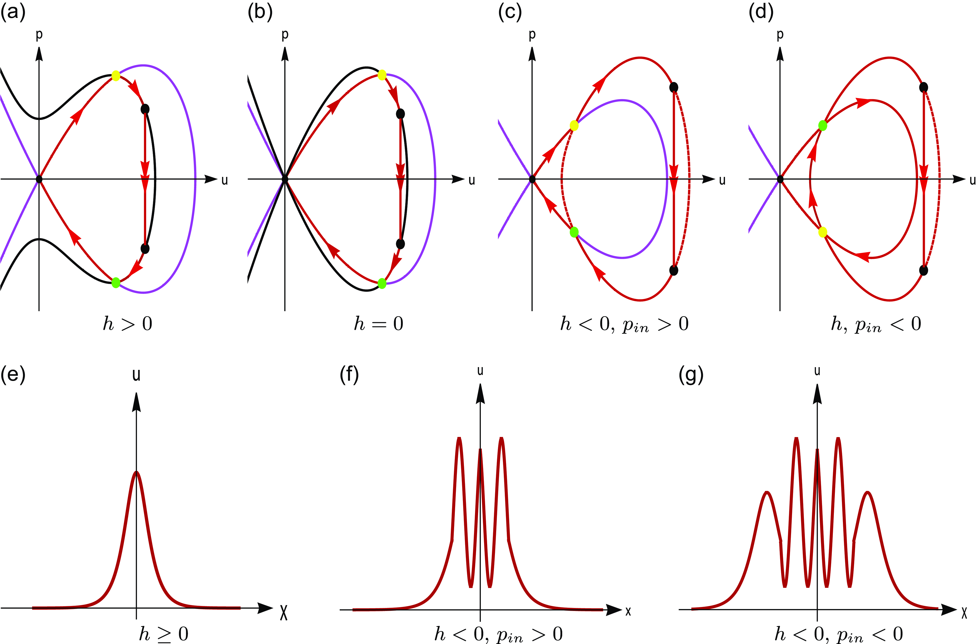
Figure 3 Long description
Panel A: A phase plane diagram shows a homoclinic orbit of the first system connecting to an open orbit of the second system defined by the energy level H=h with h greater than 0. The axes are labeled u and p. Panel B: A phase plane diagram shows homoclinic orbits of the first system connecting to a homoclinic orbit of the second system defined by H=h with h equal to 0. The axes are labeled u and p. Panel C: A phase plane diagram shows homoclinic orbits of the first system connecting to a periodic orbit of the second system defined by H=h with h less than 0 and pin greater than 0. The axes are labeled u and p. Panel D: A phase plane diagram shows homoclinic orbits of the first system connecting to a periodic orbit of the second system defined by H=h with h less than 0 and pin less than 0. The axes are labeled u and p. Panel E: A graph shows a singular pulse orbit in the (x, u) plane for h greater than or equal to 0. The axes are labeled x and u. Panel F: A graph shows a singular pulse orbit in the (x, u) plane for h less than 0 and pin greater than 0. The axes are labeled x and u. Panel G: A graph shows a singular pulse orbit in the (x, u) plane for h less than 0 and pin less than 0. The axes are labeled x and u.
(a)–(d) Sketched plots on the pinned singular homoclinic orbits $u_{p,0}(\chi )$
in the
$u_{p,0}(\chi )$
in the $(u,p)$
plane with
$(u,p)$
plane with $\sigma \lt 0$
and
$\sigma \lt 0$
and $u_0 \gt u_{in}$
. (e)–(g) Sketched plots on the pinned singular homoclinic orbits in the
$u_0 \gt u_{in}$
. (e)–(g) Sketched plots on the pinned singular homoclinic orbits in the $(\chi ,u)$
plane.
$(\chi ,u)$
plane.
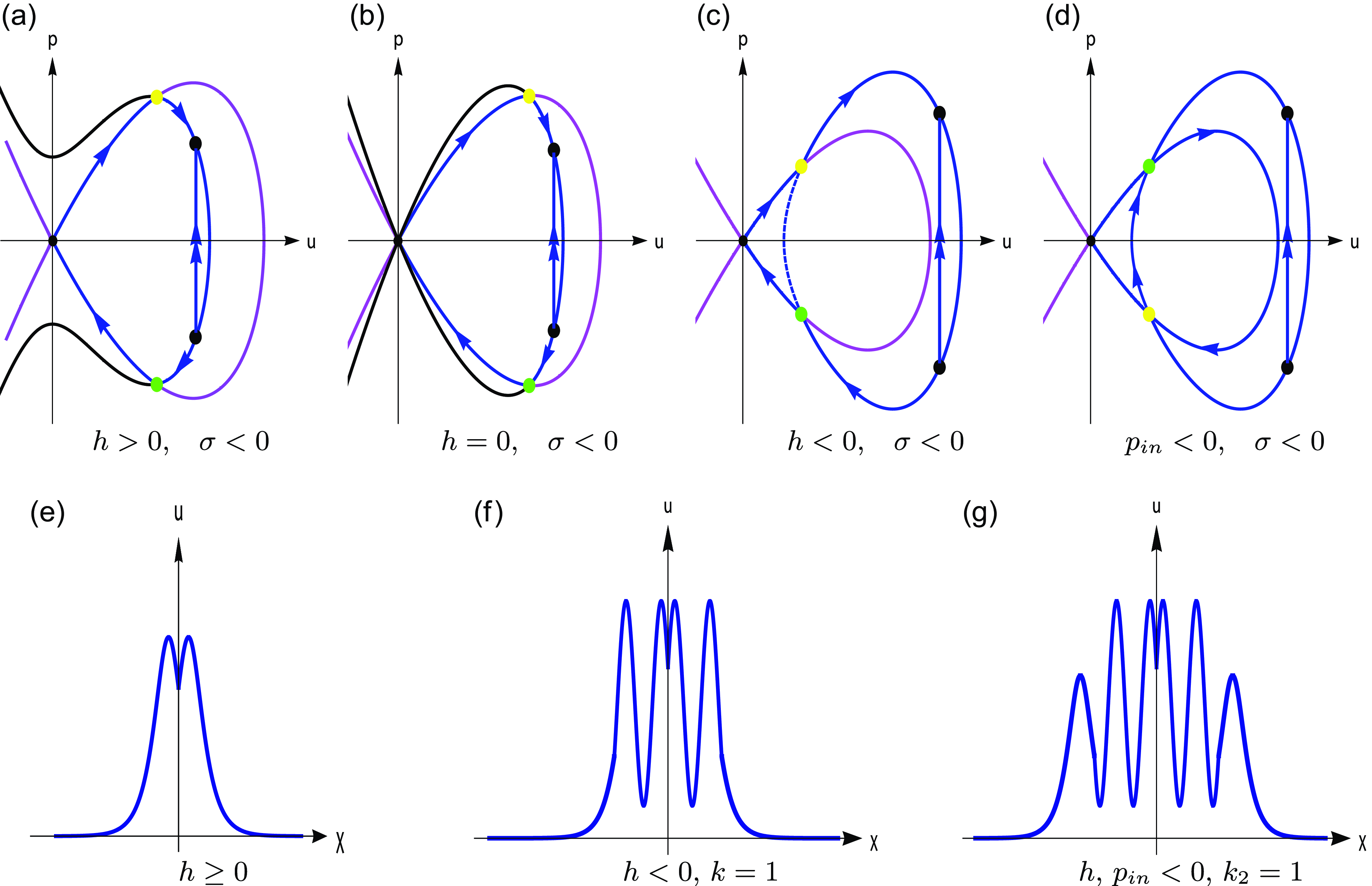
4. Proof of Theorem 2
In the previous section, we prove the existence of pinned pulse solutions $(u_{h}(x), v_{h}(x))$
to system (1.2). In this section, we analyse the (in)stability of these solutions.
$(u_{h}(x), v_{h}(x))$
to system (1.2). In this section, we analyse the (in)stability of these solutions.
Linearising equation (1.2) around $(u_{h}(x), v_{h}(x))$
yields
$(u_{h}(x), v_{h}(x))$
yields
 \begin{equation} \begin{aligned} 0 &=\bar {u}_{xx}-\left (\varepsilon ^{2} \frac {\partial ^2 }{\partial u^2}W(u_{h}(x),\chi ) - F_u(u_{h}(x),v_{h}(x))\right )\bar {u} + F_v(u_{h}(x),v_{h}(x))\bar {v},\\[5pt] 0&=\varepsilon ^{2} \bar {v}_{xx}-G_u(u_{h}(x),v_{h}(x),\varepsilon )\bar {u}- G_v(u_{h}(x),v_{h}(x),\varepsilon ) \bar {v}.\quad \quad \quad \end{aligned} \end{equation}
Then introducing the linear operator $\mathcal{L}$
gives the associated eigenvalue problem,
$\mathcal{L}$
gives the associated eigenvalue problem,
 \begin{equation} \begin{aligned} \mathcal{L} \begin{pmatrix} \bar {u}\\[5pt] \bar {v} \end{pmatrix} =\lambda \begin{pmatrix} \varepsilon ^2\bar {u}\\[5pt] \bar {v} \end{pmatrix}. \end{aligned} \end{equation}
In terms of the fast scale $\xi = x/\varepsilon$
, the eigenvalue problem turns out to be
$\xi = x/\varepsilon$
, the eigenvalue problem turns out to be
 \begin{equation} \begin{aligned} \bar {u}_{\xi \xi }&=\left [\varepsilon ^{4}\left (\frac {\partial ^2 }{\partial u^2}W(u_{h}(\xi ),\chi )+\lambda \right )+\varepsilon ^{2} F_u(u_{h}(\xi ),v_{h}(\xi ))\right ]\bar {u}+\varepsilon ^{2} F_v(u_{h}(\xi ),v_{h}(\xi ))\bar {v},\\[5pt] \quad \bar {v}_{\xi \xi }&=G_u(u_{h}(\xi ),v_{h}(\xi ),\varepsilon )\bar {u}+\big (\lambda +G_v(u_{h}(\xi ),v_{h}(\xi ),\varepsilon )\big )\bar {v}. \end{aligned} \end{equation}
Denote $\varphi (\xi )=(\bar {u}(\xi ),\, \bar {p}(\xi ),\, \bar {v}(\xi ),\, \bar {q}(\xi ))^{T}$
, then system (4.3) can be rewritten as
$\varphi (\xi )=(\bar {u}(\xi ),\, \bar {p}(\xi ),\, \bar {v}(\xi ),\, \bar {q}(\xi ))^{T}$
, then system (4.3) can be rewritten as
 \begin{equation} \varphi '=A(\xi ,\lambda ,\varepsilon )\varphi , \end{equation}
where
 \begin{equation} A (\xi ,\lambda ,\varepsilon )= \begin{pmatrix} 0\;\;\;\; & \varepsilon\;\;\;\; & 0\;\;\;\; & 0\\[5pt] Q(\xi ,\lambda ,\varepsilon )\;\;\;\; & 0\;\;\;\; &0\;\;\;\; &\varepsilon F_v(u_{h}(\xi ),v_{h}(\xi ))\\[5pt] 0\;\;\;\; & 0\;\;\;\; & 0\;\;\;\; & 1\\[5pt] G_u(u_{h}(\xi ),v_{h}(\xi ),\varepsilon )\;\;\;\; &0\;\;\;\; &\lambda +G_v(u_{h}(\xi ),v_{h}(\xi ),\varepsilon ) \;\;\;\; &0 \end{pmatrix} \end{equation}
with
 \begin{equation*}Q(\xi ,\lambda ,\varepsilon )=\varepsilon ^3\left (\frac {\partial ^2 }{\partial u^2}W(u_{h}(\xi ),\chi )+\lambda \right )+\varepsilon F_u(u_{h}(\xi ),v_{h}(\xi )).\end{equation*}
This section aims to determine the spectrum $\sigma (\mathcal{L} )$
, which consists of the essential spectrum
$\sigma (\mathcal{L} )$
, which consists of the essential spectrum $\sigma _{\textrm {ess}}(\mathcal{L} )$
and the point spectrum
$\sigma _{\textrm {ess}}(\mathcal{L} )$
and the point spectrum $\sigma _{\textrm {pt}}(\mathcal{L} )$
. According to [Reference Kapitula and Promislow20, Theorem 3.1.11], the essential spectrum consists of all the eigenvalues such that the asymptotic matrix of (4.3) is not hyperbolic. Taking the limit
$\sigma _{\textrm {pt}}(\mathcal{L} )$
. According to [Reference Kapitula and Promislow20, Theorem 3.1.11], the essential spectrum consists of all the eigenvalues such that the asymptotic matrix of (4.3) is not hyperbolic. Taking the limit $|\xi |\rightarrow \infty$
in
$|\xi |\rightarrow \infty$
in $ A (\xi ,\lambda ,\varepsilon )$
, we obtain the asymptotic matrix,
$ A (\xi ,\lambda ,\varepsilon )$
, we obtain the asymptotic matrix,
 \begin{equation} A_{\infty }(\lambda ,\varepsilon )= \begin{pmatrix} 0 & \varepsilon & 0 & 0\\[5pt] \,\varepsilon ^{3}(W^{\prime \prime }_1(0)+\lambda )\, & 0 &0 &0\\[5pt] 0 & 0 & 0 & 1\\[5pt] 0 &0 &G_v(0,0,\varepsilon )+\lambda &0 \end{pmatrix}. \end{equation}
Solving $\det |\Lambda I - A_{\infty }(\lambda , \varepsilon )| = 0$
gives the eigenvalues
$\det |\Lambda I - A_{\infty }(\lambda , \varepsilon )| = 0$
gives the eigenvalues $\Lambda _{1, 4}(\lambda )=\pm \Lambda _{f}(\lambda )$
and
$\Lambda _{1, 4}(\lambda )=\pm \Lambda _{f}(\lambda )$
and $\Lambda _{2, 3}(\lambda )=\pm \varepsilon ^2\Lambda _{s}(\lambda )$
, where
$\Lambda _{2, 3}(\lambda )=\pm \varepsilon ^2\Lambda _{s}(\lambda )$
, where
 \begin{equation} \Lambda _{f}(\lambda )=\sqrt {G_v(0,0,\varepsilon )+\lambda },\,\,\,\,\,\,\,\,\Lambda _{s}(\lambda )=\sqrt {W^{\prime \prime }_1(0)+\lambda }, \end{equation}
and the corresponding eigenvectors are
 \begin{equation} Y_{1, 4}(\lambda )=\left ( 0,\, 0,\,1, \,\pm \Lambda _{f}(\lambda )\right )^T,\,\, Y_{2, 3}(\lambda )=\left (1,\,\pm \varepsilon \Lambda _{s}(\lambda ),\, 0,\, 0\right )^T. \end{equation}
Thus, the essential spectrum of the eigenvalue problem (4.4) is
 \begin{equation} \Sigma _{\textrm {ess}}(\mathcal{L} )=\left \{\lambda \in \mathbb{C}\mid \lambda \in (\!-\infty ,-\min \{G_v(0,0,\varepsilon ),W^{\prime \prime }_1(0)\}\,]\,\right \}. \end{equation}
Under the assumptions (A1) and (A3), the essential spectrum lies entirely in the left half of the complex plane.
4.1. The Evans function
Define the complement of the essential spectrum in the complex plane $\mathbb{C}$
by
$\mathbb{C}$
by
 \begin{equation*} \mathcal{C}_e\;:\!=\;\mathbb{C}\backslash \Sigma _{\textrm {ess}}(\mathcal{L} ). \end{equation*}
Since $|\Lambda _{2,3}(\lambda )|\ll |\Lambda _{1,4}(\lambda )|$
, the solutions to the eigenvalue problem (4.3) also exhibit a slow-fast nature.
$|\Lambda _{2,3}(\lambda )|\ll |\Lambda _{1,4}(\lambda )|$
, the solutions to the eigenvalue problem (4.3) also exhibit a slow-fast nature.
Lemma 1.
For any $\lambda \in \mathcal{C}_e$
, system (4.3) has four solutions
$\lambda \in \mathcal{C}_e$
, system (4.3) has four solutions $ \{\varphi _{\pm ,v}(\xi ,\lambda ),\, \varphi _{\pm ,u}(\xi ,\lambda )\}$
satisfying the asymptotic conditions as follows:
$ \{\varphi _{\pm ,v}(\xi ,\lambda ),\, \varphi _{\pm ,u}(\xi ,\lambda )\}$
satisfying the asymptotic conditions as follows:
 \begin{equation} \begin{aligned} \lim _{\xi \rightarrow -\infty }\varphi _{+,v}(\xi ,\lambda )e^{- \Lambda _{1}(\lambda )\,\xi }=&Y_{1}(\lambda ),\\[5pt] \lim _{\xi \rightarrow -\infty }\varphi _{+,u}(\xi ,\lambda )e^{-\Lambda _{2}(\lambda )\,\xi } =& Y_{2}(\lambda ),\\[5pt] \lim _{\xi \rightarrow +\infty }\,\varphi _{-,v}(\xi ,\lambda )e^{-\Lambda _{ 4}(\lambda )\,\xi }=&Y_{4}(\lambda ),\\[5pt] \lim _{\xi \rightarrow +\infty }\,\,\varphi _{-,u}(\xi ,\lambda )e^{-\Lambda _{3}(\lambda )\,\xi } =& Y_{3}(\lambda ). \end{aligned} \end{equation}
Proof. Since $A (\xi ,\lambda ,\varepsilon )\rightarrow A_{\infty }(\lambda ,\varepsilon )$
as
$A (\xi ,\lambda ,\varepsilon )\rightarrow A_{\infty }(\lambda ,\varepsilon )$
as $\xi \rightarrow \pm \infty$
and
$\xi \rightarrow \pm \infty$
and
 \begin{equation*} \int ^{\pm \infty }_0\,\|A (\xi ,\lambda ,\varepsilon )- A_{\infty }(\lambda ,\varepsilon )\|\,\textrm {d}\xi \lt \infty , \end{equation*}
the conclusion follows directly from [Reference Coppel9, Theorem 4.1].
According to [Reference Kapitula and Promislow20], $\lambda$
is an eigenvalue of
$\lambda$
is an eigenvalue of $\mathcal{L}$
if and only if there exists a non-trivial function
$\mathcal{L}$
if and only if there exists a non-trivial function $\varphi \in \textrm{C}^1(\mathbb{R}, \mathbb{R}^4)$
solving system (4.4). By Lemma subsection 1, the solution
$\varphi \in \textrm{C}^1(\mathbb{R}, \mathbb{R}^4)$
solving system (4.4). By Lemma subsection 1, the solution $\varphi _{+,v/u}(\xi , \lambda )$
decays exponentially to
$\varphi _{+,v/u}(\xi , \lambda )$
decays exponentially to $(0, 0, 0, 0)^T$
as
$(0, 0, 0, 0)^T$
as $\xi \to -\infty$
, and
$\xi \to -\infty$
, and $\varphi _{-,v/u}(\xi , \lambda )$
decays exponentially to
$\varphi _{-,v/u}(\xi , \lambda )$
decays exponentially to $(0, 0, 0, 0)^T$
as
$(0, 0, 0, 0)^T$
as $\xi \to +\infty$
. Thus,
$\xi \to +\infty$
. Thus, $\{\varphi _{+,u}, \, \varphi _{+,v}\}$
and
$\{\varphi _{+,u}, \, \varphi _{+,v}\}$
and $\{\varphi _{-,u}, \, \varphi _{-,v}\}$
span the unstable subspace
$\{\varphi _{-,u}, \, \varphi _{-,v}\}$
span the unstable subspace $\Phi _+(\xi , \lambda )$
and the stable subspace
$\Phi _+(\xi , \lambda )$
and the stable subspace $\Phi _-(\xi , \lambda )$
, respectively. The eigenfunctions of (4.4) correspond to the intersections of these subspaces. This geometric viewpoint provides the motivation for the construction of the Evans function
$\Phi _-(\xi , \lambda )$
, respectively. The eigenfunctions of (4.4) correspond to the intersections of these subspaces. This geometric viewpoint provides the motivation for the construction of the Evans function $E(\lambda , \varepsilon )$
, which is analytic in
$E(\lambda , \varepsilon )$
, which is analytic in $\lambda$
, and whose zeros correspond to the eigenvalues of
$\lambda$
, and whose zeros correspond to the eigenvalues of $\mathcal{L}$
(counted with multiplicity). These observations lead to the following definition of the Evans function:
$\mathcal{L}$
(counted with multiplicity). These observations lead to the following definition of the Evans function:
 \begin{align} E(\lambda ,\varepsilon )=\det [\varphi _{+,v}(\xi ,\lambda ),\varphi _{+,u}(\xi ,\lambda ),\varphi _{-,u}(\xi ,\lambda ), \varphi _{-,v}(\xi ,\lambda )]. \end{align}
Consequently, the problem of identifying the eigenvalues is reduced to the location the zeros of the analytic function $E(\lambda , \varepsilon )$
(see [Reference Kapitula and Promislow20, Lemma 9.3.4]). Since
$E(\lambda , \varepsilon )$
(see [Reference Kapitula and Promislow20, Lemma 9.3.4]). Since $\Lambda _{1,4}(\lambda ) = \mathcal{O}(1)$
and
$\Lambda _{1,4}(\lambda ) = \mathcal{O}(1)$
and $\Lambda _{2,3}(\lambda ) = \mathcal{O}(\varepsilon ^2) \ll 1$
, the functions
$\Lambda _{2,3}(\lambda ) = \mathcal{O}(\varepsilon ^2) \ll 1$
, the functions $\varphi _{+,v}(\xi , \lambda )$
and
$\varphi _{+,v}(\xi , \lambda )$
and $\varphi _{-,v}(\xi , \lambda )$
are uniquely determined by their asymptotic behaviour as
$\varphi _{-,v}(\xi , \lambda )$
are uniquely determined by their asymptotic behaviour as $\xi \to -\infty$
and
$\xi \to -\infty$
and $\xi \to \infty$
.
$\xi \to \infty$
.
Since $v_{h}(\xi )$
vanishes at leading order in the slow fields, it follows that
$v_{h}(\xi )$
vanishes at leading order in the slow fields, it follows that $A (\xi ,\lambda ,\varepsilon )$
approaches a slowly varying intermediate matrix, namely,
$A (\xi ,\lambda ,\varepsilon )$
approaches a slowly varying intermediate matrix, namely,
 \begin{equation} A_{s}(\xi ,\lambda ,\varepsilon )= \begin{pmatrix} 0\;\;\;\; & \varepsilon\;\;\;\; & 0\;\;\;\; & 0\\[9pt] \varepsilon ^3\left (\dfrac {\partial ^2 }{\partial u^2}W(u_{p,0}(\xi ),\varepsilon ^2\xi )+\lambda \right )\;\;\;\; & 0\;\;\;\; &0\;\;\;\; &0\\[9pt] 0\;\;\;\; & 0\;\;\;\; & 0\;\;\;\; & 1\\[5pt] 0\;\;\;\; &0\;\;\;\; &G_v(u_{p,0}(\xi ),0,0)+\lambda\;\;\;\; &0 \end{pmatrix}. \end{equation}
We observe in (4.12) that the dynamics of the slow and fast variables have been separated. Furthermore, the distance between $A_{s}(\xi , \lambda ,\varepsilon )$
and
$A_{s}(\xi , \lambda ,\varepsilon )$
and $A_{\infty }(\lambda ,\varepsilon )$
is exponentially small.
$A_{\infty }(\lambda ,\varepsilon )$
is exponentially small.
Lemma 2. Consider
 \begin{equation} \frac{\text{d}}{\text{d} \xi }\psi =A_{s}(\xi ,\lambda ,\varepsilon )\psi ,\quad \end{equation}
where $\psi =(u,p,v,q)^T$
and
$\psi =(u,p,v,q)^T$
and $A_{s}(\xi ,\lambda ,\varepsilon )$
is given in (4.12). Let
$A_{s}(\xi ,\lambda ,\varepsilon )$
is given in (4.12). Let $\lambda \in \Omega$
, and then for
$\lambda \in \Omega$
, and then for $\xi \lt -\frac {1}{\sqrt {\varepsilon }}$
, the stable and unstable subspaces of (4.13) are, respectively, spanned by
$\xi \lt -\frac {1}{\sqrt {\varepsilon }}$
, the stable and unstable subspaces of (4.13) are, respectively, spanned by $\psi ^-_{+,u,v}(\xi ,\lambda )$
and
$\psi ^-_{+,u,v}(\xi ,\lambda )$
and $\psi ^-_{-,u,v}(\xi ,\lambda )$
, which are given by
$\psi ^-_{-,u,v}(\xi ,\lambda )$
, which are given by
 \begin{equation} \psi ^-_{\pm ,u}(\xi ,\lambda )=\left (u_{\pm }(\xi ,\lambda ),\frac {1}{\varepsilon }\frac {du_{\pm }}{d \xi }(\xi ,\lambda ),0,0\right )^T,\quad \psi ^-_{\pm ,v}(\xi ,\lambda )=\left (0,0,v_{\pm }(\xi ,\lambda ),\frac {dv_{\pm }}{d \xi }(\xi ,\lambda )\right )^T, \end{equation}
enjoying the following properties:
 \begin{equation} \begin{aligned} \lim _{\xi \rightarrow -\infty } \psi ^-_{+,u}(\xi ,\lambda )e^{-\Lambda _{2}(\lambda )\,\xi } =& Y_{2}(\lambda ),\\[5pt] \lim _{\xi \rightarrow +\infty }\psi ^-_{-,u}(\xi ,\lambda )e^{-\Lambda _{3}(\lambda )\,\xi } =& Y_{3}(\lambda ),\\[5pt] \lim _{\xi \rightarrow -\infty } \psi ^-_{+,v}(\xi ,\lambda )e^{-\Lambda _{1}(\lambda )\,\xi } =& Y_{1}(\lambda ),\\[5pt] \lim _{\xi \rightarrow +\infty }\psi ^-_{-,v}(\xi ,\lambda )e^{-\Lambda _{4}(\lambda )\,\xi } =& Y_{4}(\lambda ). \end{aligned} \end{equation}
For $\xi \gt \frac {1}{\sqrt {\varepsilon }}$
, by the reversibility symmetry, the solution spaces of (4.13) now are spanned by
$\xi \gt \frac {1}{\sqrt {\varepsilon }}$
, by the reversibility symmetry, the solution spaces of (4.13) now are spanned by $\psi ^+_{\pm ,u,v}(\xi ,\lambda )$
, where
$\psi ^+_{\pm ,u,v}(\xi ,\lambda )$
, where
 \begin{equation} \begin{aligned} \psi ^+_{\pm ,u}(\chi;\;\lambda )&=\left (u_{\mp }(\!-\xi;\;\lambda ),-\frac {1}{\varepsilon }\frac {du_{\mp }}{d \xi }(\!-\xi;\;\lambda ),0,0\right )^T,\\[5pt] \psi ^+_{\pm ,v}(\chi;\;\lambda )&=\left (0,0,v_{\mp }(\!-\xi;\;\lambda ),-\frac {dv_{\mp }}{d \xi }(\!-\xi;\;\lambda )\right )^T. \end{aligned} \end{equation}
Theorem 5. The eigenvalues are given by the zeros of the Evans function
 \begin{align} E(\lambda ,\varepsilon )&=4\,\varepsilon t_{s,+}(\lambda ,\varepsilon )t_{f,+}(\lambda ,\varepsilon )\sqrt {G_v(0,0,\varepsilon )+\lambda }\sqrt {W^{\prime \prime }_1(0)+\lambda }, \end{align}
where $t_{f,+}(\lambda ,\varepsilon )$
is an analytic transmission function and
$t_{f,+}(\lambda ,\varepsilon )$
is an analytic transmission function and $t_{s,+}(\lambda ,\varepsilon )$
is meromorphic function in
$t_{s,+}(\lambda ,\varepsilon )$
is meromorphic function in $\lambda$
. These functions are defined via the asymptotic behaviour
$\lambda$
. These functions are defined via the asymptotic behaviour
 \begin{equation} \begin{aligned} \lim _{\xi \rightarrow +\infty }\varphi _{+,v}(\xi ,\lambda )\,e^{- \Lambda _{1}(\lambda )\,\xi }\,=t_{f,+}(\lambda ,\varepsilon )Y_{1}(\lambda ),\\[5pt] \lim _{\xi \rightarrow +\infty }\varphi _{+,u}(\xi ,\lambda )\,e^{- \Lambda _{2}(\lambda )\,\xi }\,=t_{s,+}(\lambda ,\varepsilon )Y_{2}(\lambda ), \end{aligned} \end{equation}
where $\varphi _{+,v}(\xi ,\lambda )$
has been stated in Lemma subsection 1 and
$\varphi _{+,v}(\xi ,\lambda )$
has been stated in Lemma subsection 1 and $\varphi _{+,u}(\xi ,\lambda )$
is the unique solution to (4.4), provided
$\varphi _{+,u}(\xi ,\lambda )$
is the unique solution to (4.4), provided $t_{f,+}(\lambda ,\varepsilon )\neq 0$
, satisfying the boundary conditions
$t_{f,+}(\lambda ,\varepsilon )\neq 0$
, satisfying the boundary conditions
 \begin{equation} \begin{aligned} \lim _{x\rightarrow -\infty }\varphi _{+,u}(\xi ,\lambda )e^{-\Lambda _{2}(\lambda )\,\,\xi }&= Y_{2}(\lambda ),\\[5pt] \lim _{x\rightarrow +\infty }\varphi _{+,u}(\xi ,\lambda )e^{- \Lambda _{1}(\lambda )\,\xi }&=(0,0,0,0)^T. \end{aligned} \end{equation}
Moreover, there exists a meromorphic transmission function $t_{s,-}(\lambda ,\varepsilon )$
such that, to leading order,
$t_{s,-}(\lambda ,\varepsilon )$
such that, to leading order,
 \begin{equation} \varphi _{+,u}(\xi ,\lambda )= \begin{cases} \psi ^-_{+,u}(\xi ,\lambda ), \quad \quad \quad &\xi \lt -\dfrac {1}{\sqrt {\varepsilon }},\\[10pt] t_{s,+}(\lambda ,\varepsilon )\psi ^-_{-,u}(\!-\xi ,\lambda ) +t_{s,-}(\lambda ,\varepsilon )\psi ^-_{+,u}(\!-\xi ,\lambda ), \quad &\xi \,\,\gt \,\,\dfrac {1}{\sqrt {\varepsilon }}. \end{cases} \end{equation}
Proof. It follows from (3.34) that there are two positive, $\mathcal{O}(1)$
constants
$\mathcal{O}(1)$
constants $C_1$
and
$C_1$
and $C_2$
such that
$C_2$
such that
 \begin{equation*}\|A (\xi ,\lambda ,\varepsilon )- A_{s}(\xi ,\lambda ,\varepsilon )\|\leq C_1\textrm {e}^{-C_2|\xi |}\end{equation*}
for $\xi \in I_{s}^\pm$
. Hence, to leading order,
$\xi \in I_{s}^\pm$
. Hence, to leading order, $\psi _{\pm ,v}(\xi , \lambda )$
and
$\psi _{\pm ,v}(\xi , \lambda )$
and $\psi _{\pm ,u}(\xi , \lambda )$
can be selected as basis solutions to (4.4). According to the asymptotics of
$\psi _{\pm ,u}(\xi , \lambda )$
can be selected as basis solutions to (4.4). According to the asymptotics of $\varphi _{+,v}(\xi ,\lambda )$
as
$\varphi _{+,v}(\xi ,\lambda )$
as $\xi \rightarrow -\infty$
, we know that it remains exponentially close to
$\xi \rightarrow -\infty$
, we know that it remains exponentially close to $\psi _{+,v}(\xi ,\lambda )$
for
$\psi _{+,v}(\xi ,\lambda )$
for $\xi \lt -\frac {1}{\sqrt {\varepsilon }}$
. Although the exact form of
$\xi \lt -\frac {1}{\sqrt {\varepsilon }}$
. Although the exact form of $\varphi _{+,v}(\xi ,\lambda )$
is unknown, to leading order, it can be written as
$\varphi _{+,v}(\xi ,\lambda )$
is unknown, to leading order, it can be written as
 \begin{equation*} \varphi _{+,v}(\xi ,\lambda )=t_{f,+}(\lambda )\psi ^+_{+,v}(\xi )+t_{f,-}(\lambda )\psi ^+_{-,v}(\xi )+t_{+}(\lambda )\psi ^+_{+,u}(\xi )+t_{-}(\lambda )\psi ^+_{-,u}(\xi ) \end{equation*}
for $\xi \gt \frac {1}{\sqrt {\varepsilon }}$
. This proves the first result in (4.18). In order to determine
$\xi \gt \frac {1}{\sqrt {\varepsilon }}$
. This proves the first result in (4.18). In order to determine $\varphi _{+,u}(\xi )$
uniquely, it can be found that
$\varphi _{+,u}(\xi )$
uniquely, it can be found that $\varphi _{+,u}(\xi ,\lambda )$
grows obeying the speed of
$\varphi _{+,u}(\xi ,\lambda )$
grows obeying the speed of $\mathcal{O}(\textrm {e}^{\Lambda _{2}(\lambda )\,\,\xi })$
. That is,
$\mathcal{O}(\textrm {e}^{\Lambda _{2}(\lambda )\,\,\xi })$
. That is, $\varphi _{+,u}(\xi ,\lambda )$
must satisfy (4.19) if
$\varphi _{+,u}(\xi ,\lambda )$
must satisfy (4.19) if $t_{f,+}(\lambda )\neq 0$
. Hence, similar to
$t_{f,+}(\lambda )\neq 0$
. Hence, similar to $\varphi _{+,v}(\xi ,\lambda )$
, we obtain (4.20) accordingly.
$\varphi _{+,v}(\xi ,\lambda )$
, we obtain (4.20) accordingly.
By Liouville’s formula and $\textrm {Tr}\textrm {A}(x)=\Sigma _{i=1}^4 \Lambda _{i}(\lambda )$
, the Evans function turns out to be
$\textrm {Tr}\textrm {A}(x)=\Sigma _{i=1}^4 \Lambda _{i}(\lambda )$
, the Evans function turns out to be
 \begin{align*} E(\lambda ,\varepsilon )&=\lim _{\xi \rightarrow +\infty }\det [\varphi _{+,v}(\xi ,\lambda ),\varphi _{+,u}(\xi ,\lambda ),\varphi _{-,u}(\xi ,\lambda ), \varphi _{-,v}(\xi ,\lambda )]e^{-\int ^{x}_{0}Tr \textrm {A}(x)dx}\\[5pt] &=\lim _{\xi \rightarrow +\infty }\det \big[\varphi _{+,v}(\xi ,\lambda )e^{-\Lambda _{1}(\lambda )\xi },\varphi _{+,u}(\xi ,\lambda )e^{-\Lambda _{2}(\lambda )\xi }, \varphi _{-,u}(\xi ,\lambda )e^{-\Lambda _{3}(\lambda )\xi },\varphi _{-,v}(\xi ,\lambda )e^{-\Lambda _{4}(\lambda )\xi }\big]\\[5pt] &=\det [t_{f,+}(\lambda ,\varepsilon )Y_{1}(\lambda ),t_{s,+}(\lambda ,\varepsilon )Y_{2}(\lambda ),Y_{3}(\lambda ),Y_{4}(\lambda )]\\[5pt] &=4\varepsilon t_{s,+}(\lambda ,\varepsilon )t_{f,+}(\lambda ,\varepsilon ) \sqrt {G_v(0,0,\varepsilon )+\lambda }\sqrt {W^{\prime \prime }_1(0)+\lambda }. \end{align*}
As a consequence, the eigenvalues of (4.3) are exactly identical with the roots of $t_{s,+}(\lambda ,\varepsilon )$
or
$t_{s,+}(\lambda ,\varepsilon )$
or $t_{f,+}(\lambda ,\varepsilon )$
. Nevertheless, we will also see that some roots of
$t_{f,+}(\lambda ,\varepsilon )$
. Nevertheless, we will also see that some roots of $t_{f,+}(\lambda ,\varepsilon )$
may not correspond to the true eigenvalues, as
$t_{f,+}(\lambda ,\varepsilon )$
may not correspond to the true eigenvalues, as $t_{s,+}(\lambda ,\varepsilon )$
may possess poles at these values, which cancel the zeros.
$t_{s,+}(\lambda ,\varepsilon )$
may possess poles at these values, which cancel the zeros.
4.2.
The fast transmission function
$t_{f,+}(\lambda ,\varepsilon )$

In this section, we determine the zeros of the fast transmission function $t_{f,+}(\lambda ,\varepsilon ).$
Let $\varepsilon \rightarrow 0$
in system (4.3), we get
$\varepsilon \rightarrow 0$
in system (4.3), we get
 \begin{equation} (\mathcal{L}_f-\lambda ) v=G_u(u_{0},v_{0}(\xi ),0)\,\bar {u}(0),\quad \quad \mathcal{L}_fv:v_{\xi \xi }-G_v(u_{0},v_{0}(\xi ),0)\,v, \end{equation}
which is a second-order inhomogeneous differential equation. Here, we have used the fact that $u_h(\xi )=u_0$
and
$u_h(\xi )=u_0$
and $v_h(\xi )=v_{0}(\xi )$
for
$v_h(\xi )=v_{0}(\xi )$
for $\xi \in I_f$
as
$\xi \in I_f$
as $\varepsilon \rightarrow 0$
. Equation (4.21) corresponds to the fast limiting eigenvalue problem in the singular limit of system (4.3), which is a classical Sturm–Liouville eigenvalue problem. Thus, by Sturm–Liouville theory, the eigenvalues of
$\varepsilon \rightarrow 0$
. Equation (4.21) corresponds to the fast limiting eigenvalue problem in the singular limit of system (4.3), which is a classical Sturm–Liouville eigenvalue problem. Thus, by Sturm–Liouville theory, the eigenvalues of $\mathcal{L}_f$
can be enumerated in a strictly descending order,
$\mathcal{L}_f$
can be enumerated in a strictly descending order,
 \begin{equation*}\lambda ^f_{0}\gt \lambda ^f_{1}=0\gt \cdots \gt \lambda ^f_{N}\gt -G_v(u_{0},0,0).\end{equation*}
Moreover, the eigenfunction $\bar {v}_i(\xi )$
corresponding to
$\bar {v}_i(\xi )$
corresponding to $\lambda ^f_{i}$
has exactly
$\lambda ^f_{i}$
has exactly $i$
distinct zeroes and is even or odd depending on whether
$i$
distinct zeroes and is even or odd depending on whether $i$
is even or odd, respectively.
$i$
is even or odd, respectively.
The homogeneous problem associated with system (4.21) can be written as
 \begin{equation} \frac{\text{d}}{\text{d} \xi }\phi =A_{f}(\xi ,\lambda )\phi ,\quad \end{equation}
where $\phi =(v,q)^T$
and
$\phi =(v,q)^T$
and $A_{f}(\xi , \lambda )$
is a
$A_{f}(\xi , \lambda )$
is a $2\times 2$
matrix, which is exactly the lower
$2\times 2$
matrix, which is exactly the lower $2\times 2$
block of
$2\times 2$
block of $A(\xi , \lambda ,\varepsilon )$
in the limit
$A(\xi , \lambda ,\varepsilon )$
in the limit $\varepsilon \rightarrow 0.$
Obviously, system (4.22) has two solutions
$\varepsilon \rightarrow 0.$
Obviously, system (4.22) has two solutions $\phi _{+}(\xi , \lambda )$
,
$\phi _{+}(\xi , \lambda )$
, $\phi _{-}(\xi , \lambda )$
satisfying
$\phi _{-}(\xi , \lambda )$
satisfying
 \begin{equation} \begin{aligned} \lim _{\xi \rightarrow -\infty }\phi _{+}(\xi , \lambda )e^{- \Lambda _{1}(\lambda )\,\xi }=(1,\Lambda _{1}(\lambda ))^T, \quad \quad \quad \lim _{\xi \rightarrow +\infty }\,\phi _{-}(\xi , \lambda )e^{-\Lambda _{ 4}(\lambda )\,\xi }=(1,\Lambda _{4}(\lambda ))^T, \end{aligned} \end{equation}
and there exists an analytic function $t_{f}(\lambda )$
such that
$t_{f}(\lambda )$
such that
 \begin{equation} \lim _{\xi \rightarrow +\infty }\,\phi _{+}(\xi ,\lambda )e^{-\Lambda _{ 1}(\lambda )\,\xi }=t_{f}(\lambda )(1,\Lambda _{1}(\lambda ))^T. \end{equation}
The Evans function associated with this problem is given by
 \begin{align} \begin{aligned} E_f(\lambda )=\lim _{\xi \rightarrow +\infty }\det [\phi _{+}(\xi ,\lambda ),\phi _{-}(\xi ,\lambda )] =\det [t_{f}(\lambda )(1,\Lambda _{1}(\lambda ))^T,(1,\Lambda _{4}(\lambda ))^T]=-2t_{f}(\lambda )\Lambda _{1}(\lambda ). \end{aligned} \end{align}
By construction, the leading order behaviour of $t_{f,+}(\lambda ,\varepsilon )$
is determined by
$t_{f,+}(\lambda ,\varepsilon )$
is determined by $t_{f}(\lambda )$
. It thus follows from (4.25) that
$t_{f}(\lambda )$
. It thus follows from (4.25) that $t_{f}(\lambda )=0$
if and only if
$t_{f}(\lambda )=0$
if and only if $E_{f}(\lambda )=0$
. Hence, the eigenvalues of (4.22) correspond to the zeros of
$E_{f}(\lambda )=0$
. Hence, the eigenvalues of (4.22) correspond to the zeros of $t_{f}(\lambda )=0$
. That is, the roots of the function
$t_{f}(\lambda )=0$
. That is, the roots of the function $t_{f}(\lambda )$
are given by
$t_{f}(\lambda )$
are given by $\lambda ^f_{i}$
,
$\lambda ^f_{i}$
, $i=0,1,\ldots ,N$
.
$i=0,1,\ldots ,N$
.
Lemma 3.
Let $0\lt \varepsilon \ll 1$
, then the fast transmission function is given by
$0\lt \varepsilon \ll 1$
, then the fast transmission function is given by
 \begin{equation} t_{f,+}(\lambda ,\varepsilon )=\tilde {t}_f(\lambda ,\varepsilon ) \prod _{i=1}^{n}\left (\lambda -\lambda ^f_{i}(\varepsilon )\right ) \end{equation}
with $\tilde {t}_f(\lambda ,\varepsilon )\neq 0$
, and
$\tilde {t}_f(\lambda ,\varepsilon )\neq 0$
, and $\lambda ^f_{i}(\varepsilon )$
has the following regular expansion:
$\lambda ^f_{i}(\varepsilon )$
has the following regular expansion:
 \begin{equation} \lambda ^f_{i}(\varepsilon )=\lambda ^f_{i}+\varepsilon ^2 \lambda ^f_{i,1}+\mathcal{O}(\varepsilon ^4), \end{equation}
for $i=0,1,\ldots ,N.$
The proof of this lemma is analogous to those in [Reference Doelman, Gardner and Kaper12–Reference Doelman, Iron and Nishiura14] by using the ‘elephant trunk’ procedure [Reference Alexander, Gardner and Jones1, Reference Gardner and Jones18]. It is important to note that $\lambda ^f_{1}(\varepsilon )\equiv 0$
is no longer valid since system (1.2) now is non-autonomous, leading to the loss of translational invariance. As a result, under the perturbation, the eigenvalue
$\lambda ^f_{1}(\varepsilon )\equiv 0$
is no longer valid since system (1.2) now is non-autonomous, leading to the loss of translational invariance. As a result, under the perturbation, the eigenvalue $\lambda ^f_{1}(\varepsilon )$
may be shifted to the one having the positive real part. Under certain situations, standard perturbation methods such as the Lin–Sandstede method [Reference Bastiaansen, Chirilus-Bruckner and Doelman3, Reference Kapitula and Promislow20, Reference Li and Yu23] can be applied to estimate the location of these eigenvalues. However, due to the piecewise-smooth nature of system (1.2), no effective methods currently exist for precisely determining the location of these eigenvalues.
$\lambda ^f_{1}(\varepsilon )$
may be shifted to the one having the positive real part. Under certain situations, standard perturbation methods such as the Lin–Sandstede method [Reference Bastiaansen, Chirilus-Bruckner and Doelman3, Reference Kapitula and Promislow20, Reference Li and Yu23] can be applied to estimate the location of these eigenvalues. However, due to the piecewise-smooth nature of system (1.2), no effective methods currently exist for precisely determining the location of these eigenvalues.
Remark 11. While the Lin–Sandstede method can be used to detect the eigenvalue bifurcating from $\lambda = 0$
under perturbations, its validity depends heavily on the assumption that the eigenfunction associated with the perturbed eigenvalue remains a small deformation of the unperturbed one. This assumption enables a regular perturbation approach, where a solvability condition – typically of Fredholm type – is imposed to determine the first-order correction
$\lambda = 0$
under perturbations, its validity depends heavily on the assumption that the eigenfunction associated with the perturbed eigenvalue remains a small deformation of the unperturbed one. This assumption enables a regular perturbation approach, where a solvability condition – typically of Fredholm type – is imposed to determine the first-order correction $\lambda =\lambda _1^f(\varepsilon )$
. However, in the singularly perturbed system studied here, this assumption does not hold. As shown in the previous section, the pulse solution undergoes a transition when it passes the interfaces at
$\lambda =\lambda _1^f(\varepsilon )$
. However, in the singularly perturbed system studied here, this assumption does not hold. As shown in the previous section, the pulse solution undergoes a transition when it passes the interfaces at $\chi =\pm L$
. Consequently, the eigenfunction associated with
$\chi =\pm L$
. Consequently, the eigenfunction associated with $\lambda = \lambda _1^f(\varepsilon )$
does not converge to the eigenfunction associated with
$\lambda = \lambda _1^f(\varepsilon )$
does not converge to the eigenfunction associated with $\lambda = 0$
as
$\lambda = 0$
as $\varepsilon \to 0$
. So Lin–Sandstede method is not applicable here. We adopt an alternative technique to study the spectrum of the linearised operator.
$\varepsilon \to 0$
. So Lin–Sandstede method is not applicable here. We adopt an alternative technique to study the spectrum of the linearised operator.
Although $\lambda ^f_0(\varepsilon )$
is a simple zero of the function
$\lambda ^f_0(\varepsilon )$
is a simple zero of the function $t_{f,+}(\lambda , \varepsilon )$
, this does not imply that the function
$t_{f,+}(\lambda , \varepsilon )$
, this does not imply that the function $E(\lambda , \varepsilon )$
also vanishes at this point. This is due to the fact that
$E(\lambda , \varepsilon )$
also vanishes at this point. This is due to the fact that $\lambda = \lambda ^f_0(\varepsilon )$
is a first-order pole of the transmission function
$\lambda = \lambda ^f_0(\varepsilon )$
is a first-order pole of the transmission function $t_{s,+}(\lambda )$
and therefore cannot be an eigenvalue of the full system. This phenomenon is known as the ‘NLEP Paradox’ in literature.
$t_{s,+}(\lambda )$
and therefore cannot be an eigenvalue of the full system. This phenomenon is known as the ‘NLEP Paradox’ in literature.
According to (4.23)–(4.24), we know that $\phi _{+}(\xi ,\lambda )$
and
$\phi _{+}(\xi ,\lambda )$
and $\phi _{-}(\xi ,\lambda )$
form a fundamental set of linearly independent solutions to the homogeneous system (4.22) for
$\phi _{-}(\xi ,\lambda )$
form a fundamental set of linearly independent solutions to the homogeneous system (4.22) for $\lambda \neq \lambda ^f_{i}$
,
$\lambda \neq \lambda ^f_{i}$
, $i=0,1,\ldots N$
. Consequently, by employing the method of constant variation we can derive a bounded solution to the heterogeneous problem (4.21).
$i=0,1,\ldots N$
. Consequently, by employing the method of constant variation we can derive a bounded solution to the heterogeneous problem (4.21).
Lemma 4.
For $\lambda \neq \lambda ^f_{i}$
,
$\lambda \neq \lambda ^f_{i}$
, $i=0,1,\ldots N$
, the unique bounded solution
$i=0,1,\ldots N$
, the unique bounded solution $v_{in}(\xi ,\lambda )$
to the inhomogeneous problem (4.21) is given by
$v_{in}(\xi ,\lambda )$
to the inhomogeneous problem (4.21) is given by
 \begin{align} \begin{aligned} v_{in}(\xi ,\lambda )&= \frac {\bar {u}(0)}{E_f(\lambda )} \left (v_{-}(\xi , \lambda )\int ^{\xi }_{-\infty } G_u(u_{0},v_{0}(s),0)v_{+}(s, \lambda )\, \textrm {d}s\right .\\[5pt] & \quad + \left .v_{+}(\xi , \lambda )\int _{\xi }^{+\infty } G_u(u_{0},v_{0}(s),0)v_{-}(s, \lambda )\,\textrm {d}s\right ), \end{aligned} \end{align}
where $v_{\pm }(\xi , \lambda )$
is the
$v_{\pm }(\xi , \lambda )$
is the $v$
-component of
$v$
-component of $\phi _{\pm }(\xi , \lambda )=(v_{\pm }(\xi , \lambda ),q_{\pm }(\xi , \lambda ))$
, and
$\phi _{\pm }(\xi , \lambda )=(v_{\pm }(\xi , \lambda ),q_{\pm }(\xi , \lambda ))$
, and $E_f(\lambda )$
is defined as in (4.25).
$E_f(\lambda )$
is defined as in (4.25).
Lemma 5.
(See [Reference de Rijk, Doelman and Rademacher10]) The bounded solution $v_{in}(\xi , \cdot )$
is meromorphic in the region
$v_{in}(\xi , \cdot )$
is meromorphic in the region $\mathcal{C}_e$
for fixed
$\mathcal{C}_e$
for fixed $\xi \in \mathbb{R}$
and analytic on
$\xi \in \mathbb{R}$
and analytic on $\mathcal{C}_e\backslash \{\lambda ^f_{i}\}_{i=0}^N$
for
$\mathcal{C}_e\backslash \{\lambda ^f_{i}\}_{i=0}^N$
for $\xi \in \mathbb{R}$
. Furthermore, when
$\xi \in \mathbb{R}$
. Furthermore, when $i$
is even,
$i$
is even, $\lambda =\lambda ^f_{i}$
is a pole of
$\lambda =\lambda ^f_{i}$
is a pole of $v_{in}(\xi , \lambda )$
, while when
$v_{in}(\xi , \lambda )$
, while when $i$
is odd, it is a removable singularity.
$i$
is odd, it is a removable singularity.
Proof. Since $\mathcal{L}_f - \lambda$
is a Fredholm operator of index zero for
$\mathcal{L}_f - \lambda$
is a Fredholm operator of index zero for $\lambda \in \mathcal{C}_e$
, and
$\lambda \in \mathcal{C}_e$
, and $\mathcal{L}_f - \lambda$
is invertible if and only if
$\mathcal{L}_f - \lambda$
is invertible if and only if $\lambda \in \mathcal{C}_e\backslash \{\lambda ^f_{i}\}_{i=0}^N$
, it follows that
$\lambda \in \mathcal{C}_e\backslash \{\lambda ^f_{i}\}_{i=0}^N$
, it follows that $(\mathcal{L}_f - \lambda )^{-1}$
is analytic on
$(\mathcal{L}_f - \lambda )^{-1}$
is analytic on $\mathcal{C}_e\backslash \{\lambda ^f_{i}\}_{i=0}^N$
and meromorphic on the entire region
$\mathcal{C}_e\backslash \{\lambda ^f_{i}\}_{i=0}^N$
and meromorphic on the entire region $\mathcal{C}_e$
. Since
$\mathcal{C}_e$
. Since $\mathcal{L}_f - \lambda$
is a self-adjoint operator, it follows from the Fredholm alternative [Reference Kapitula and Promislow20, Theorem 2.2.1] that a bounded solution to the inhomogeneous equation exists at
$\mathcal{L}_f - \lambda$
is a self-adjoint operator, it follows from the Fredholm alternative [Reference Kapitula and Promislow20, Theorem 2.2.1] that a bounded solution to the inhomogeneous equation exists at $\lambda \in \{\lambda ^f_{i}\}_{i=0}^N$
if and only if the following solvability condition is satisfied:
$\lambda \in \{\lambda ^f_{i}\}_{i=0}^N$
if and only if the following solvability condition is satisfied:
 \begin{equation*} \int _{-\infty }^{+\infty } G_u(u_{0},v_{0}(\xi ),0)\bar {v}_{i}(\xi , \lambda ) \,\textrm {d}\xi =0, \end{equation*}
where $\bar {v}_{i}(\xi , \lambda )\in \ker (\mathcal{L}_f-\lambda )$
. According to Sturm–Liouville theory, if
$\bar {v}_{i}(\xi , \lambda )\in \ker (\mathcal{L}_f-\lambda )$
. According to Sturm–Liouville theory, if $i$
is even, the corresponding eigenfunction
$i$
is even, the corresponding eigenfunction $\bar {v}_i(\xi )$
is an even function, and if
$\bar {v}_i(\xi )$
is an even function, and if $i$
is odd, it is an odd function. Since the homoclinic solution
$i$
is odd, it is an odd function. Since the homoclinic solution $v_0(\xi )$
is even, the solvability condition does not hold when
$v_0(\xi )$
is even, the solvability condition does not hold when $i$
is even. Therefore,
$i$
is even. Therefore, $\lambda = \lambda ^f_{i}$
is a pole of
$\lambda = \lambda ^f_{i}$
is a pole of $v_{in}(\xi , \lambda )$
. When
$v_{in}(\xi , \lambda )$
. When $i$
is odd, the solvability condition holds, and
$i$
is odd, the solvability condition holds, and $\lambda =\lambda ^f_{i}$
is a removable singularity.
$\lambda =\lambda ^f_{i}$
is a removable singularity.
Remark 12. The bounded solution $v_{in}(\xi ,\lambda )$
to the inhomogeneous problem (4.21) forms one of the key ingredients of the slow transmission function
$v_{in}(\xi ,\lambda )$
to the inhomogeneous problem (4.21) forms one of the key ingredients of the slow transmission function $t_{s,+}(\lambda ,\varepsilon )$
(see the subsequent subsection).
$t_{s,+}(\lambda ,\varepsilon )$
(see the subsequent subsection).
4.3.
The slow transmission function
$t_{s,+}(\lambda ,\varepsilon )$

We will see that the slow transmission function $t_{s,+}(\lambda ,\varepsilon )$
can be determined by matching the slow and fast orbits, respectively, of the following slow limit eigenvalue problem:
$t_{s,+}(\lambda ,\varepsilon )$
can be determined by matching the slow and fast orbits, respectively, of the following slow limit eigenvalue problem:
 \begin{equation} \left \{ {\begin{array}{l} u_{\chi }=p,\\[5pt] p_{\chi }=\left (W(u_{p,0}(\chi ),\chi )+\lambda \right )u, \end{array}} \right . \end{equation}
and the fast limit eigenvalue problem (4.21).
Recall that, on the slow intervals $I_s^{\pm }$
,
$I_s^{\pm }$
,
 \begin{equation*} \psi ^+_{\pm ,u}(\xi ,\lambda ) = \left ( u_{\pm }(\xi ,\lambda ), \frac {1}{\varepsilon } \frac {du_{\pm }}{d \xi }(\xi ,\lambda ), 0, 0 \right ).\end{equation*}
To simplify the notation and to enhance the clarity of formulation, we utilise the variable $\chi =\varepsilon ^2 \xi$
and define
$\chi =\varepsilon ^2 \xi$
and define $ (u_{\pm }(\chi , \lambda ), p_{\pm }(\chi , \lambda ))$
.
$ (u_{\pm }(\chi , \lambda ), p_{\pm }(\chi , \lambda ))$
.
Denote
 \begin{equation*} \psi ^+_{\pm ,u}(\chi ,\lambda ) = \left ( u_{\pm }(\chi , \lambda ), \varepsilon p_{\pm }(\chi , \lambda ), 0, 0 \right ) \end{equation*}
with $p_{\pm }(\chi , \lambda )=\frac{\text{d}}{\text{d}\chi }u_{\pm }(\chi , \lambda )$
; thus,
$p_{\pm }(\chi , \lambda )=\frac{\text{d}}{\text{d}\chi }u_{\pm }(\chi , \lambda )$
; thus, $\left (u_{\pm }(\chi , \lambda ), p_{\pm }(\chi , \lambda )\right )$
is the unique solution to the slow limit eigenvalue problem (4.29) satisfying
$\left (u_{\pm }(\chi , \lambda ), p_{\pm }(\chi , \lambda )\right )$
is the unique solution to the slow limit eigenvalue problem (4.29) satisfying
 \begin{equation*} \lim _{\chi \rightarrow \mp \infty }( u_{\pm }(\chi , \lambda ), p_{\pm }(\chi , \lambda ))\textrm {e}^{\mp \Lambda _s(\lambda )\chi } =(1,\,\pm \Lambda _s(\lambda )). \end{equation*}
Lemma 6.
Define $u_{\pm }(0, \lambda )=u_{\pm }(\chi =0)$
and
$u_{\pm }(0, \lambda )=u_{\pm }(\chi =0)$
and $p_{\pm }(0, \lambda )=p_{\pm }(\chi =0)$
, then the leading order of the slow transmission function can be given by
$p_{\pm }(0, \lambda )=p_{\pm }(\chi =0)$
, then the leading order of the slow transmission function can be given by
 \begin{equation} \begin{aligned} t_{s,+}(\lambda ) =-\frac {\Big (u_+(0, \lambda ) \mathcal{G}(\lambda )+2p_+(0, \lambda )\Big )u_+(0, \lambda )}{u_+(0, \lambda ) p_-(0, \lambda )-u_-(0, \lambda )p_+(0, \lambda )}, \end{aligned} \end{equation}
where
 \begin{equation} \mathcal{G}(\lambda )=\int ^{+\infty }_{-\infty }\int ^{\xi }_{-\infty }\Big (F_u(u_{0},v_{0}(\xi )+\frac {F_v(u_{0},v_{0}(\xi ))}{E_f(\lambda )} G_u(u_{0},v_{0}(s),0)v_{+}(s, \lambda )v_{-}(\xi , \lambda )\Big )\,\textrm {d}s\,\textrm {d}\xi . \end{equation}
Proof. It follows from Theorem 5 that there exists a positive constant $K$
independent of
$K$
independent of $\varepsilon$
such that
$\varepsilon$
such that
 \begin{equation*} \varphi _{+,u}(\xi , \lambda )=\psi ^-_{+,u}(\xi ,\lambda )+\mathcal{O}(e^{-K\xi }), \end{equation*}
for $\xi \in I_s^-$
, and
$\xi \in I_s^-$
, and
 \begin{equation*} \varphi _{+,u}(\xi , \lambda )=t_{s,+}(\lambda , \varepsilon )\psi ^+_{+,u}(\xi , \lambda ) +t_{s,-}(\lambda , \varepsilon )\psi ^+_{-,u}(\xi , \lambda )+\mathcal{O}(e^{-K\xi }) \end{equation*}
for $\xi \in I_s^+$
. Accordingly, we can determine the explicit representation of
$\xi \in I_s^+$
. Accordingly, we can determine the explicit representation of $t_{s,+}(\lambda ,\varepsilon )$
by matching the fast and slow orbits. More precisely, to compute
$t_{s,+}(\lambda ,\varepsilon )$
by matching the fast and slow orbits. More precisely, to compute $t_{s,+}(\lambda , \varepsilon )$
, we need to track the changes of
$t_{s,+}(\lambda , \varepsilon )$
, we need to track the changes of $\bar {u}_{+}(\xi , \lambda )$
and
$\bar {u}_{+}(\xi , \lambda )$
and $\bar {p}_{+}(\xi , \lambda )$
during the fast transition, that is,
$\bar {p}_{+}(\xi , \lambda )$
during the fast transition, that is, $\xi \in I_f$
.
$\xi \in I_f$
.
We define the slow difference function $\Delta _s$
by
$\Delta _s$
by
 \begin{equation} \Delta _s\left (\begin{array}{l} \bar {u }\\[5pt] \bar {p} \\[5pt] \bar {v }\\[5pt] \bar {q} \end{array}\right )=\lim _{\xi \downarrow \frac {1}{\sqrt {\varepsilon }}}\Big (t_{s,+}(\lambda ,\varepsilon )\psi ^-_{-,u}(\!-\xi;\;\lambda ) +t_{s,-}(\lambda ,\varepsilon )\psi ^-_{+,u}(\!-\xi;\;\lambda )\Big ) -\lim _{\xi \uparrow -\frac {1}{\sqrt {\varepsilon }}} \psi ^-_{+,u}(\xi ,\lambda ). \end{equation}
First, it follows from (4.4) that $\bar {u}_+(\xi , \lambda )$
remains constant to leading order during the fast field
$\bar {u}_+(\xi , \lambda )$
remains constant to leading order during the fast field $I_f$
. As a consequence,
$I_f$
. As a consequence,
 \begin{equation} \bar {u}_+\left (\!-\frac {1}{\sqrt {\varepsilon }}\right )= \bar {u}_+\left (\frac {1}{\sqrt {\varepsilon }}\right )+\mathcal{O}(\varepsilon ^{3/2}). \end{equation}
This together with
 \begin{equation} \bar {u}\left (\!-\frac {1}{\sqrt {\varepsilon }}\right )=u_+(0,\lambda )+\mathcal{O}(\varepsilon ^{3/2}) \end{equation}
gives
 \begin{equation} \bar {u}\left (\frac {1}{\sqrt {\varepsilon }}\right ) =t_{s,+}(\lambda )u_-(0,\lambda )+t_{s,-}(\lambda )u_+(0,\lambda )+\mathcal{O}(\varepsilon ^{3/2}). \end{equation}
Thus, the first matching condition (4.33) can be written as
 \begin{equation} u_+(0,\lambda ) =t_{s,+}(\lambda )u_-(0,\lambda )+ t_{s,-}(\lambda )u_+(0,\lambda ). \end{equation}
So the first relation between $t_{s,+}(\lambda )$
and
$t_{s,+}(\lambda )$
and $t_{s,-}(\lambda )$
can be given by
$t_{s,-}(\lambda )$
can be given by
 \begin{equation} t_{s,-}(\lambda )=1-\frac {u_-(0,\lambda )}{u_+(0,\lambda )}t_{s,+}(\lambda ). \end{equation}
On the other hand, the derivative $\bar {p}_{+}(\xi , \lambda )$
changes rapidly in the fast field
$\bar {p}_{+}(\xi , \lambda )$
changes rapidly in the fast field $I_f$
. It can be determined through the following two ways. First, we use the information on
$I_f$
. It can be determined through the following two ways. First, we use the information on $\varphi _{+,u}(\xi , \lambda )$
in the slow field to compute it. The change
$\varphi _{+,u}(\xi , \lambda )$
in the slow field to compute it. The change $\Delta _{s}\bar {p}$
, to leading order, can be approximated by the difference of
$\Delta _{s}\bar {p}$
, to leading order, can be approximated by the difference of $\bar {p}_{+}(\xi , \lambda )$
between two ends of the slow field, that is,
$\bar {p}_{+}(\xi , \lambda )$
between two ends of the slow field, that is,
 \begin{align} \begin{aligned} \Delta _{s}\bar {p}&= \bar {p}_{+}\left (\frac {1}{\sqrt {\varepsilon }}\right )- \bar {p}_{+}\left (\!-\frac {1}{\sqrt {\varepsilon }}\right )\\[5pt] &=\frac {1}{\varepsilon }\left (t_{s,+}(\lambda )\frac{\text{d}}{\text{d}\xi }u_-(\!-\xi )+ t_{s,-}(\lambda )\left .\frac{\text{d}}{\text{d}\xi }u_+(\!-\xi )\right )\right |_{\xi =\frac {1}{\sqrt {\varepsilon }}} -\frac {1}{\varepsilon } \left .\frac{\text{d}}{\text{d}\xi }u_+(\xi ) \right |_{\xi =-\frac {1}{\sqrt {\varepsilon }}}\\[5pt] &=-\frac {1}{\varepsilon }\left (t_{s,+}(\lambda )\frac{\text{d}}{\text{d}\xi }u_-(\xi )+ t_{s,-}(\lambda )\left .\frac{\text{d}}{\text{d}\xi }u_+(\xi ) +\frac{\text{d}}{\text{d}\xi }u_+(\xi )\right )\right |_{\xi =-\frac {1}{\sqrt {\varepsilon }}}\\[5pt] &=-\frac {1}{\varepsilon }\left (t_{s,+}(\lambda )\frac{\text{d}}{\text{d}\xi }u_-(\xi )+ \left (1-\frac {u_-(0)}{u_+(0)}t_{s,+}(\lambda )\right )\left .\frac{\text{d}}{\text{d}\xi }u_+(\xi ) +\frac{\text{d}}{\text{d}\xi }u_+(\xi )\right )\right |_{\xi =-\frac {1}{\sqrt {\varepsilon }}}\\[5pt] &=-\varepsilon \left [\left (\frac{\text{d}}{\text{d}\chi }u_-(\chi ) -\frac {u_-(0)\frac{\text{d}}{\text{d}\chi }u_+(\chi )}{u_+(0)}t_{s,+}(\lambda )\right )\left . +2\frac{\text{d}}{\text{d}\chi }u_+(\chi )\right ]\right |_{\chi =-\varepsilon ^{3/2}}\\[5pt] &=-\varepsilon \left ( \frac {u_+(0)p_-(0)-u_-(0)p_+(0)}{u_+(0)}t_{s,+}(\lambda ) +2p_+(0)\right ). \end{aligned} \end{align}
Second, the accumulated jump concerning the first-order derivative can be obtained by integrating $\overline {u}_{\xi \xi }$
over the fast field, that is, to leading order,
$\overline {u}_{\xi \xi }$
over the fast field, that is, to leading order,
 \begin{equation} \begin{aligned} \Delta _{f}\,\bar {p}&=\frac {1}{\varepsilon }\int _{I_f}\bar {u}_{\xi \xi }\,\textrm {d}\xi \\[5pt] &=\varepsilon \int ^{+\infty }_{-\infty }\Big ( F_u(u_{0},v_{0}(\xi )\bar {u}(0)+F_v(u_{0},v_{0}(\xi ))v_{in}(\xi , \lambda )\Big )\,\textrm {d}\xi ,\\[5pt] &= \varepsilon u_+(0)\int ^{+\infty }_{-\infty }\int ^{\xi }_{-\infty }\Big (F_u(u_{0},v_{0}(\xi )+\frac {F_v(u_{0},v_{0}(\xi ))}{E_f(\lambda )} G_u(u_{0},v_{0}(s),0)v_{+}(s;\;\lambda )v_{-}(\xi , \lambda )\Big )\,\textrm {d}s\,\textrm {d}\xi . \end{aligned} \end{equation}
By combining (4.38) and (4.39), one can get (4.30) up to the leading order.
Remark 13. It is worthy to note that only the roots of $t_{s,+}(\lambda ,0)$
are not sufficient to decide the spectral stability of the pinned pulse of (1.2) due to the fact that the sign of
$t_{s,+}(\lambda ,0)$
are not sufficient to decide the spectral stability of the pinned pulse of (1.2) due to the fact that the sign of $\lambda ^f_{1}(\varepsilon )$
cannot be determined.
$\lambda ^f_{1}(\varepsilon )$
cannot be determined.
Remark 14. If $F_v(u,v)\equiv 0$
for all
$F_v(u,v)\equiv 0$
for all $u,\,v\gt 0$
, then
$u,\,v\gt 0$
, then
 \begin{equation*} \mathcal{G}(\lambda )=\int ^{+\infty }_{-\infty }\int ^{\xi }_{-\infty } F_u(u_{0},v_{0}(\xi )) \,\textrm {d}s \,\textrm {d}\xi , \end{equation*}
which implies that the transmission function $t_{s,+}(\lambda ,\varepsilon )$
is only determined by the slow reduced eigenvalues problem (4.29). As a consequence,
$t_{s,+}(\lambda ,\varepsilon )$
is only determined by the slow reduced eigenvalues problem (4.29). As a consequence, $t_{s,+}(\lambda ,\varepsilon )$
is analytic on
$t_{s,+}(\lambda ,\varepsilon )$
is analytic on $\mathcal{C}_e$
, and the zeros of
$\mathcal{C}_e$
, and the zeros of $t_{f,+}(\lambda ,\varepsilon )$
cannot be cancelled by the poles of
$t_{f,+}(\lambda ,\varepsilon )$
cannot be cancelled by the poles of $t_{s,+}(\lambda ,\varepsilon )$
. In this case, we conclude that the linearised eigenvalue problem can be completely separated into the slow and fast reduced eigenvalue problems without the interaction between them. Thus, the zeros of
$t_{s,+}(\lambda ,\varepsilon )$
. In this case, we conclude that the linearised eigenvalue problem can be completely separated into the slow and fast reduced eigenvalue problems without the interaction between them. Thus, the zeros of $t_{f,+}(\lambda ,\varepsilon )$
with positive real parts yield the spectral instability directly.
$t_{f,+}(\lambda ,\varepsilon )$
with positive real parts yield the spectral instability directly.
5. (In)stability of pinned pulses in non-autonomous GM equation
Consider
 \begin{equation} \left \{ {\begin{array}{l} \varepsilon ^{2}U_{t}= U_{xx}-\varepsilon ^{2}\Big (f(\chi ) U-g(\chi ) U^d\Big )+\sigma V^{2},\\[5pt] \,\,\,V_{t}=\varepsilon ^{2}V_{xx}-V+\frac {V^{2}}{U}, \end{array}} \right . \end{equation}
whose existence has been set up in Section 3. The associated eigenvalue problem is
 \begin{equation} \varphi '=A(\xi ,\lambda ,\varepsilon )\varphi , \end{equation}
where $\varphi (\xi )=(\bar {u}(\xi ), \bar {p}(\xi ), \bar {v}(\xi ), \bar {q}(\xi ))^{T}$
, and
$\varphi (\xi )=(\bar {u}(\xi ), \bar {p}(\xi ), \bar {v}(\xi ), \bar {q}(\xi ))^{T}$
, and
 \begin{equation} A (\xi ,\lambda ,\varepsilon )= \begin{pmatrix} 0\;\;\;\; & \varepsilon\;\;\;\; & 0\;\;\;\; & 0\\[5pt] \varepsilon ^3(f(\chi )-dg(\chi )u^{d-1}_{h}(\varepsilon ^2\xi )+\lambda )\;\;\;\; & 0\;\;\;\; &-2\varepsilon \sigma v_{h}(\xi )\;\;\;\; &0\\[5pt] 0\;\;\;\; & 0\;\;\;\; & 0\;\;\;\; & 1\\[9pt] \dfrac {v^2_{h}(\xi )}{ u^2_{h}(\varepsilon ^2\xi )}\;\;\;\; &0\;\;\;\; &1+\lambda -\dfrac {2v_{h}^{2}(\xi )}{u_{h}(\varepsilon ^2\xi )}\;\;\;\; &0 \end{pmatrix}. \end{equation}
By (5.2), the essential spectrum turns out to be
 \begin{equation} \Sigma _{ess}=\left \{\lambda \in \mathbb{C}\mid \lambda \in (\!-\infty ,-\min \{1,\alpha _1\}]\right \}. \end{equation}
Now (4.21) becomes
 \begin{equation} (\mathcal{L}_f-\lambda ) v=\frac {v^2_{0}(\xi )}{ u^2_{0}}\bar {u}(0),\quad \quad \mathcal{L}_fv\;:\!=\;v_{\xi \xi }-\left (1-\frac {2v_{0}(\xi )}{u_{0}}\right )v. \end{equation}
Obviously, the eigenvalues associated with the operator $\mathcal{L}_f$
are well-known, namely,
$\mathcal{L}_f$
are well-known, namely, $\lambda ^f_{0}=5/4$
,
$\lambda ^f_{0}=5/4$
, $\lambda ^f_{1}=0$
and
$\lambda ^f_{1}=0$
and $\lambda ^f_{2}=-3/4$
.
$\lambda ^f_{2}=-3/4$
.
As treated in [Reference Veerman and Doelman37], we can obtain the following result.
Lemma 7.
For $0\lt \varepsilon \ll 1$
, the fast transmission function can be given by
$0\lt \varepsilon \ll 1$
, the fast transmission function can be given by
 \begin{equation} t_{f,+}(\lambda ,\varepsilon )=\tilde {t}_f(\lambda ,\varepsilon ) \left (\lambda -\lambda ^f_{0}(\varepsilon )\right )\left (\lambda -\lambda ^f_{1}(\varepsilon )\right ) \left (\lambda -\lambda ^f_{2}(\varepsilon )\right ) \end{equation}
with $\tilde {t}_f(\lambda ,\varepsilon )\neq 0$
, and
$\tilde {t}_f(\lambda ,\varepsilon )\neq 0$
, and $\lambda ^f_{i}(\varepsilon )$
has the following regular expansion:
$\lambda ^f_{i}(\varepsilon )$
has the following regular expansion:
 \begin{equation} \lambda ^f_{i}(\varepsilon )=\lambda ^f_{i}+\varepsilon ^2 \lambda ^f_{i,1}+\mathcal{O}(\varepsilon ^4), \quad i=0,1,2. \end{equation}
In particular, for $\lambda \neq \lambda ^f_{i}, i=0,1,2$
, the unique solution of
$\lambda \neq \lambda ^f_{i}, i=0,1,2$
, the unique solution of $v_{in}(\xi ,\lambda )$
to the heterogeneous problem (4.21) now is
$v_{in}(\xi ,\lambda )$
to the heterogeneous problem (4.21) now is
 \begin{equation} v_{in}(\zeta ,\lambda )= 9\bar {u}(0) \Big [v_{+}(\zeta ,\lambda )\int ^{\zeta }_{-1} (1-s^2)v_{-}(s, \lambda )\,\textrm {d}s+ v_{-}(\zeta , \lambda )\int ^{\zeta }_{-1} (1-s^2)v_{+}(s,\lambda )\,\textrm {d}s\Big ], \end{equation}
where $v_{\pm }(\zeta , \lambda )=c_{\pm }(\lambda )P_3^{-2\sqrt {1+\lambda }}\left (\pm \zeta \right )$
,
$v_{\pm }(\zeta , \lambda )=c_{\pm }(\lambda )P_3^{-2\sqrt {1+\lambda }}\left (\pm \zeta \right )$
, $\zeta =\tanh \frac {\xi }{2}$
,
$\zeta =\tanh \frac {\xi }{2}$
, $P_3^{-2\sqrt {1+\lambda }}\left (\pm \zeta \right )$
are the Legendre functions and
$P_3^{-2\sqrt {1+\lambda }}\left (\pm \zeta \right )$
are the Legendre functions and $c_{+}(\lambda )c_{-}(\lambda )=-\frac {1}{2}\Gamma (4+2\sqrt {1+\lambda })\Gamma (\!-3+2\sqrt {1+\lambda })$
.
$c_{+}(\lambda )c_{-}(\lambda )=-\frac {1}{2}\Gamma (4+2\sqrt {1+\lambda })\Gamma (\!-3+2\sqrt {1+\lambda })$
.
Lemma 8.
Concerning (5.1), the integral $\mathcal{G}(\lambda )$
defined in (4.31) now is
$\mathcal{G}(\lambda )$
defined in (4.31) now is
 \begin{equation} \mathcal{G}(\lambda )=-108\sigma u_0 \mathcal{R}(\lambda ) \end{equation}
with
 \begin{equation} \mathcal{R}(\lambda )=\int ^{1}_{-1}\int ^{\zeta }_{-1} v_{+}(\zeta ,\lambda )v_{-}(s,\lambda )(1-s^2)\,\operatorname{d}s\,\operatorname{d}\zeta . \end{equation}
By Lemma 2, we denote $u_{\pm }(\chi ,\lambda )$
the solutions to the following equation:
$u_{\pm }(\chi ,\lambda )$
the solutions to the following equation:
 \begin{equation} \quad u_{\chi \chi }=\left (\alpha _i-d\gamma _i u^{d-1}_{p,0}(\chi )+\lambda \right )u \end{equation}
with the boundary condition $\lim _{\chi \rightarrow -\infty }u_{\pm }(\chi )\textrm {e}^{\mp \sqrt {\alpha _1+\lambda }\chi }=1$
. It then follows from Theorem 2 that
$\lim _{\chi \rightarrow -\infty }u_{\pm }(\chi )\textrm {e}^{\mp \sqrt {\alpha _1+\lambda }\chi }=1$
. It then follows from Theorem 2 that $t_{s,+}(\lambda )=0$
if and only if
$t_{s,+}(\lambda )=0$
if and only if $u_+(0,\lambda )=0$
or
$u_+(0,\lambda )=0$
or
 \begin{equation*} -54\sigma u_0 \mathcal{R}(\lambda )+\frac {p_+(0,\lambda )}{ u_+(0,\lambda )}=0. \end{equation*}
Theorem 6. Let the conditions in Theorem 3 be satisfied, then
-
(i) When
$u_{0}(h)=u^+_{0}(h)$
, if
(5.12)admits
\begin{equation} \begin{aligned} \sqrt {\frac {\alpha _2+\lambda }{\alpha _2+\sqrt {\alpha _2^2+72\sigma ^2h}}}\left (1-\frac {2} {\left (1+\frac {2}{\sqrt {\frac {\alpha _2+\lambda }{\alpha _1+\lambda }}-1}\right )\textrm { e}^{2\sqrt {\alpha _2+\lambda }}+1}\right ) = 9 \sqrt {2} \mathcal{R}(\lambda ) \end{aligned} \end{equation}
$\lambda \in \{\lambda \mid \text{Re}\, \lambda \gt 0\}$
, then the pinned pulse in equation (5.1) is unstable.
-
(ii) When
$u_{0}(h)=u^-_{0}(h)$
, if
(5.13)admits
\begin{equation} \begin{aligned} \sqrt {\frac {\alpha _2 + \lambda }{\alpha _2 - \sqrt {\alpha _2^2 + 72 \sigma ^2 h}}} \left ( 1 - \frac {2}{\left (1 + \frac {2}{\sqrt {\frac {\alpha _2 + \lambda }{\alpha _1 + \lambda }} - 1}\right ) e^{2 \sqrt {\alpha _2 + \lambda }} + 1}\right ) = 9 \sqrt {2} \mathcal{R}(\lambda ) \end{aligned} \end{equation}
$\lambda \in \{\lambda \mid \text{Re}\, \lambda \gt 0\}$
, then the pinned pulse in equation (5.1) is unstable.






Proof. Now equation (5.11) turns out to be
 \begin{equation} \quad u_{\chi \chi }=(\,f(\chi )+\lambda )u. \end{equation}
Hence,
 \begin{align} u_{+}(\chi , \lambda ) = \left \{ \begin{aligned} &e^{\sqrt {\alpha _1+\lambda }\,\chi },\quad \quad \quad &\chi \lt -L,\quad \\[5pt] &M_1e^{\sqrt {\alpha _2+\lambda }\,\chi }+N_1e^{-\sqrt {\alpha _2+\lambda }\,\chi },\quad \quad \quad &-L\lt \chi \lt 0, \end{aligned}\right . \end{align}
and
 \begin{align} u_{-}(\chi , \lambda ) = \left \{ \begin{aligned} &e^{-\sqrt {\alpha _1+\lambda }\,\chi },\quad \quad \quad &\chi \lt -L,\quad \\[5pt] &M_2e^{\sqrt {\alpha _2+\lambda }\,\chi }+N_2e^{-\sqrt {\alpha _2+\lambda }\,\chi },\quad \quad \quad &-L\lt \chi \lt 0. \end{aligned}\right . \end{align}
We choose the free parameters $M_i, N_i, i=1, 2$
such that
$M_i, N_i, i=1, 2$
such that $u_{\pm }(\chi , \lambda )$
is continuously differentiable at
$u_{\pm }(\chi , \lambda )$
is continuously differentiable at $\chi =-L$
. Consequently,
$\chi =-L$
. Consequently,
 \begin{equation} \begin{pmatrix} e^{-\sqrt {\alpha _2+\lambda }\,L} & e^{\sqrt {\alpha _2+\lambda }\,L} \\[5pt] -\sqrt {\alpha _2+\lambda }\, e^{-\sqrt {\alpha _2+\lambda }\,L}& \sqrt {\alpha _2+\lambda }\, e^{\sqrt {\alpha _2+\lambda }\,L}\\[5pt] \end{pmatrix} \begin{pmatrix} M_{1}\\[5pt] N_{1}\\[5pt] \end{pmatrix} =\begin{pmatrix} e^{-\sqrt {\alpha _1+\lambda }\,L}\\[5pt] -\sqrt {\alpha _1+\lambda }\,e^{-\sqrt {\alpha _1+\lambda }\,L} \end{pmatrix}, \end{equation}
and further by the reversibility symmetry, we get
 \begin{align} \begin{aligned} M_1&=N_2=\frac {\left (\sqrt {\alpha _1+\lambda }+\sqrt {\alpha _2+\lambda }\right ) e^{\left (\sqrt {\alpha _2+\lambda }-\sqrt {\alpha _1+\lambda }\right )\,L}}{2\sqrt {\alpha _2+\lambda }},\\[5pt] N_1&=M_2=\frac {\left (\sqrt {\alpha _2+\lambda }-\sqrt {\alpha _1+\lambda }\right ) e^{-\left (\sqrt {\alpha _1+\lambda }+\sqrt {\alpha _2+\lambda }\right )\,L}}{2\sqrt {\alpha _2+\lambda }}. \end{aligned} \end{align}
This results in $u_+(0, \lambda )=M_1+N_1\neq 0$
and
$u_+(0, \lambda )=M_1+N_1\neq 0$
and
 \begin{equation*} \begin{aligned} \frac {p_+(0, \lambda )}{u_+(0, \lambda )}=\sqrt {\alpha _2+\lambda }\left (1-\frac {2} {\frac {\sqrt {\alpha _2+\lambda }+\sqrt {\alpha _1+\lambda }}{\sqrt {\alpha _2+\lambda }-\sqrt {\alpha _1+\lambda }}\textrm { e}^{2\sqrt {\alpha _2+\lambda }}+1}\right ). \end{aligned} \end{equation*}
Combining (3.12) with (5.9) gives
 \begin{align} \mathcal{G}(\lambda ) = \left \{ \begin{aligned} & -18\sqrt {2}\left (\alpha _2+\sqrt {\alpha _2^2+72\sigma ^2h}\,\right )^\frac {1}{2} \mathcal{R}(\lambda ),\quad \quad \quad &u_{0}(h)=u^+_{0}(h),\\[5pt] \ & -18\sqrt {2}\left (\alpha _2-\sqrt {\alpha _2^2+72\sigma ^2h}\,\right )^\frac {1}{2} \mathcal{R}(\lambda ), & u_{0}(h)=u^-_{0}(h) . \end{aligned}\right . \end{align}
Based on the results of Theorem 2, we accordingly get (5.12) and (5.13).
Theorem 7.
Let $\varepsilon \gt 0$
be sufficiently small, and let
$\varepsilon \gt 0$
be sufficiently small, and let $\alpha _1$
,
$\alpha _1$
, $\alpha _2\gt 0$
,
$\alpha _2\gt 0$
, $\gamma _1,\,L\gt 0$
,
$\gamma _1,\,L\gt 0$
, $\gamma _2=0$
and
$\gamma _2=0$
and $d\gt 1$
be fixed such that equation (5.1) admits a pinned pulse solution, then this pulse is unstable if
$d\gt 1$
be fixed such that equation (5.1) admits a pinned pulse solution, then this pulse is unstable if
 \begin{align} \begin{aligned} P_\nu ^{\mu }\big (z_L\big ) +\frac {\textrm{P}(\lambda )}{\sqrt {\alpha _2+\lambda }} \tanh \sqrt {\alpha _2+\lambda }\,L=0 \end{aligned} \end{align}
or
 \begin{equation} \begin{aligned} -9\sqrt {2}\mathcal{R}(\lambda )+\sqrt {\frac {\alpha _2+\lambda }{\alpha _2\pm \sqrt {\alpha _2^2+72\sigma ^2h}}}\cdot \frac {P_\nu ^{\mu }\big (z_L\big ) \tanh \sqrt {\alpha _2+\lambda }\,L +\frac {\textrm{P}(\lambda )}{\sqrt {\alpha _2+\lambda }}}{P_\nu ^{\mu }\big (z_L\big ) +\frac {\textrm{P}(\lambda )}{\sqrt {\alpha _2+\lambda }} \tanh \sqrt {\alpha _2+\lambda }\,L}=0, \end{aligned} \end{equation}
possesses $\lambda \in \{\lambda \mid \text{Re}\,\lambda \gt 0 \}$
, where
$\lambda \in \{\lambda \mid \text{Re}\,\lambda \gt 0 \}$
, where
 \begin{equation*} \begin{aligned} \textrm{P}(\lambda )&\;:\!=\;\frac {(1-d)\sqrt {\alpha _1}}{2}\left ( (\nu -\mu )P_{\nu -1}^{-\mu }\big (z_L\big )+z_L \nu P_{\nu }^{-\mu }\big (z_L\big )\right ),\\[5pt] z_L&\;:\!=\; \tanh \left (\frac {1}{2}(d-1)\sqrt {\alpha _1}(L+\textrm {sign}(p_{in})x_*)\right ). \end{aligned} \end{equation*}
in which $P_\nu ^\mu (z)$
and
$P_\nu ^\mu (z)$
and $P_\nu ^\mu (\!-z)$
are the Legendre functions and
$P_\nu ^\mu (\!-z)$
are the Legendre functions and $x_*$
is defined by (3.25).
$x_*$
is defined by (3.25).
Proof. In the slow interval $(\!-\infty ,-L)$
, to leading order, equation (5.11) is governed by
$(\!-\infty ,-L)$
, to leading order, equation (5.11) is governed by
 \begin{equation} \quad u_{\chi \chi }=\left (\alpha _1+\lambda -d\gamma _1 u^{d-1}_{h,-}(\chi )\right )u, \end{equation}
whose solution is denoted by $u_{h,-}(\chi )$
,
$u_{h,-}(\chi )$
,
Introducing the Hopf-cole transformation
 \begin{equation} z(\chi )=\tanh \left (\frac {1}{2}(d-1)\sqrt {\alpha }(\chi -\textrm {sign}(p_{in})x_*)\right ) \end{equation}
to equation (5.22) yields the Legendre differential equation,
 \begin{equation} (1-z^2)u_{zz}-2zu_z+\left (\nu (\nu +1)-\frac {\mu ^2}{1-z^2}\right )u=0, \end{equation}
where
 \begin{equation} \nu =\frac {d+1}{d-1},\quad \quad \quad \quad \mu =\frac {2}{d-1}\sqrt {1+\frac {\lambda }{\alpha _1}}. \end{equation}
The solutions of (5.24) can be given in terms of the Legendre functions $P_\nu ^\mu (z)$
and
$P_\nu ^\mu (z)$
and $P_\nu ^\mu (\!-z)$
. In light of the results in Lemma 2, we have
$P_\nu ^\mu (\!-z)$
. In light of the results in Lemma 2, we have
 \begin{equation} \begin{aligned} u_+(\chi )=&\Gamma (1+\mu )e^{-\Lambda _3(\lambda ) x_*}P_\nu ^{-\mu }\big (\!-z(\chi )\big )\\[5pt] =&e^{\sqrt {\alpha _1+\lambda }\chi }F\bigg (\nu +1,-\nu , 1+\mu , \frac {1}{2}+\frac {1}{2}z(\chi )\bigg ) \end{aligned} \end{equation}
satisfying $u_+(\chi )\rightarrow 0$
as
$u_+(\chi )\rightarrow 0$
as $\chi \rightarrow -\infty .$
To further simplify the notation, let us introduce
$\chi \rightarrow -\infty .$
To further simplify the notation, let us introduce
 \begin{align} \begin{aligned} u(\!-L, \lambda )\;:\!=\;&\lim _{\chi \uparrow -L}u_+(\chi )=\Gamma (1+\mu )e^{-\Lambda _3(\lambda ) x_*}P_\nu ^{\mu }\big (z_L\big ),\\[5pt] p(\!-L, \lambda )\;:\!=\;&\lim _{\chi \uparrow -L}p_+(\chi )= \frac {(1-d)\sqrt {\alpha _1}}{2}\Gamma (1+\mu )e^{-\Lambda _3(\lambda ) x_*} \left [ (\nu -\mu )P_{\nu -1}^{-\mu }\big (z_L\big )+z_L \nu P_{\nu }^{-\mu }\big (z_L\big )\right ], \end{aligned} \end{align}
in which
 \begin{equation*} z_L\;:\!=\;\tanh \left (\frac {1}{2}(d-1)\sqrt {\alpha }(L+\textrm {sign}(p_{in})x_*)\right ). \end{equation*}
Moreover, by following Lemma 6, we have
 \begin{align} u_{+}(\chi , \lambda ) = \left \{ \begin{aligned} &\Gamma (1+\mu )e^{-\Lambda _3(\lambda ) x_*}P_\nu ^{-\mu }\big (\!-z(\chi )\big ),\quad \quad \quad &\chi \lt -L,\quad \\[5pt] &M_3e^{\sqrt {\alpha _2+\lambda }\,\chi }+N_3e^{-\sqrt {\alpha _2+\lambda }\,\chi },\quad \quad \quad &-L\lt \chi \lt 0, \end{aligned}\right . \end{align}
where
 \begin{align} \begin{aligned} M_3&=\frac {u(\!-L,\lambda )\sqrt {\alpha _2+\lambda }+p(\!-L,\lambda )}{2\sqrt {\alpha _2+\lambda }}\textrm { e}^{\sqrt {\alpha _2+\lambda }\,L},\\[5pt] N_3&=\frac {u(\!-L,\lambda )\sqrt {\alpha _2+\lambda }-p(\!-L,\lambda )}{2\sqrt {\alpha _2+\lambda }}\textrm { e}^{-\sqrt {\alpha _2+\lambda }\,L}. \end{aligned} \end{align}
As a consequence,
 \begin{align} \begin{aligned} u_+(0,\lambda ) &=u(\!-L, \lambda ) \cosh \sqrt {\alpha _2+\lambda }\,L +\frac {p(\!-L, \lambda )}{\sqrt {\alpha _2+\lambda }} \sinh \sqrt {\alpha _2+\lambda }\,L,\\[5pt] p_+(0,\lambda ) &=u(\!-L, \lambda )\sqrt {\alpha _2+\lambda } \sinh \sqrt {\alpha _2+\lambda }\,L +p(\!-L,\lambda ) \cosh \sqrt {\alpha _2+\lambda }\,L. \end{aligned} \end{align}
This means that $u_+(0,\lambda )p_-(0,\lambda )-u_-(0,\lambda )p_+(0,\lambda )=2\sqrt {\alpha _2+\lambda }(N_3^2-M_3^2)\neq 0$
and
$u_+(0,\lambda )p_-(0,\lambda )-u_-(0,\lambda )p_+(0,\lambda )=2\sqrt {\alpha _2+\lambda }(N_3^2-M_3^2)\neq 0$
and
 \begin{align} \begin{aligned} \frac {p_+(0,\lambda )}{u_+(0,\lambda )} =\frac {\sqrt {\alpha _2+\lambda } \tanh \sqrt {\alpha _2+\lambda }\,L +\frac {p(\!-L, \lambda )}{u(\!-L,\lambda )}}{1+\frac {p(\!-L, \lambda )}{u(\!-L, \lambda )\sqrt {\alpha _2+\lambda }} \tanh \sqrt {\alpha _2+\lambda }\,L}. \end{aligned} \end{align}
Define two functions $\textrm{B}_{\pm }(\chi )$
and their derivatives
$\textrm{B}_{\pm }(\chi )$
and their derivatives $\textrm{B}^{\prime }_{\pm }(\chi )$
, respectively, by
$\textrm{B}^{\prime }_{\pm }(\chi )$
, respectively, by
 \begin{equation} \begin{aligned} \textrm{B}_{\pm }(\chi )=e^{\pm \sqrt {\alpha _2+\lambda }\chi }F\bigg (\nu +1,-\nu , 1+\mu _2, \frac {1}{2}\pm \frac {1}{2}y(\chi )\bigg ), \quad \quad \textrm{B}^{\prime }_{\pm }(\chi )=\frac{\text{d}}{\text{d}\chi }\mathcal{B}_{\pm }(\chi ). \end{aligned} \end{equation}
Theorem 8.
Let the conditions in Theorem
4
be fulfilled. If the length of the heterogeneity $L$
satisfies
$L$
satisfies $h(L)=\mathcal{O}(\varepsilon )$
, then the pinned pulse solution of equation (5.1) is unstable if
$h(L)=\mathcal{O}(\varepsilon )$
, then the pinned pulse solution of equation (5.1) is unstable if $\lambda \in \{\lambda \,|\,\text{Re}\,\lambda \gt 0 \,\}$
,
$\lambda \in \{\lambda \,|\,\text{Re}\,\lambda \gt 0 \,\}$
,
 \begin{align} \begin{aligned} u(\!-L, \lambda )\textrm{B}_2(\lambda ) + p(\!-L, \lambda ) \textrm{B}_1(\lambda )=0 \end{aligned} \end{align}
or
 \begin{equation} \begin{aligned} \frac {u(\!-L, \lambda )\textrm{B}_4(\lambda ) + p(\!-L, \lambda ) \textrm{B}_3(\lambda )} {u(\!-L, \lambda )\textrm{B}_2(\lambda ) + p(\!-L, \lambda ) \textrm{B}_1(\lambda )}=18\sqrt {\alpha _2} y_0 \mathcal{R}(\lambda ) \end{aligned} \end{equation}
admits a root $\lambda$
with positive real part, where
$\lambda$
with positive real part, where $u(\!-L, \lambda )$
and
$u(\!-L, \lambda )$
and $p(\!-L, \lambda )\,$
are defined in equation (5.27), and
$p(\!-L, \lambda )\,$
are defined in equation (5.27), and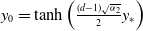 $y_0=\tanh \left (\frac {(d-1)\sqrt {\alpha _2}}{2}y_*\right )$
. Furthermore, the functions
$y_0=\tanh \left (\frac {(d-1)\sqrt {\alpha _2}}{2}y_*\right )$
. Furthermore, the functions $\textrm{B}_1(\lambda ),$ $i=1,2,3,4$
, are given by
$i=1,2,3,4$
, are given by
 \begin{equation*} \begin{aligned} \textrm{B}_1(\lambda )&=\textrm{B}_{+}(\!-L)\textrm{B}_{-}(0)-\textrm{B}_{-}(\!-L) \textrm{B}_{+}(0),\\[5pt] \textrm{B}_2(\lambda )&=\textrm{B}^{\prime }_{-}(\!-L) \textrm{B}_{+}(0)-\textrm{B}^{\prime }_{+}(\!-L)\textrm{B}_{-}(0),\\[5pt] \textrm{B}_3(\lambda )&=\textrm{B}_{+}(\!-L)\textrm{B}^{\prime }_{-}(0)-\textrm{B}_{-}(\!-L) \textrm{B}^{\prime }_{+}(0),\\[5pt] \textrm{B}_4(\lambda )&=\textrm{B}^{\prime }_{-}(\!-L) \textrm{B}^{\prime }_{+}(0)-\textrm{B}^{\prime }_{+}(\!-L)\textrm{B}^{\prime }_{-}(0). \end{aligned} \end{equation*}
Proof. First, let us consider the simple case, namely, $h(L)=0$
. In this case, equation (5.11) can be written as
$h(L)=0$
. In this case, equation (5.11) can be written as
 \begin{equation} u_{\chi \chi } = \left \{ \begin{aligned} &\left (\alpha _1+\lambda -d\gamma _1 u^{d-1}_{h,-}\big (\chi \big )\right )u,\quad \quad &\chi \in (\!-\infty ,-L),\\[5pt] &\left (\alpha _2+\lambda -d\gamma _2 u^{d-1}_{i,-}\big (\chi ,0 \big )\right )u, &\chi \in \,\,(\,-L,\,0), \end{aligned}\right . \end{equation}
where the solutions $u_{i,-}(\chi ,0 )$
and
$u_{i,-}(\chi ,0 )$
and $u_{h,-}(\chi )$
are defined in equation (3.25) and (3.27), respectively. According to the result of Lemma 7, the solution
$u_{h,-}(\chi )$
are defined in equation (3.25) and (3.27), respectively. According to the result of Lemma 7, the solution $u_{+}(\xi , \lambda )$
is given by
$u_{+}(\xi , \lambda )$
is given by
 \begin{align} u_{+}(\xi , \lambda ) = \left \{ \begin{aligned} &\Gamma (1+\mu )e^{-\Lambda _3(\lambda ) x_*}P_\nu ^{-\mu }\big (\!-z(\chi )\big ),\quad \quad \quad &\chi \lt -L,\quad \\[5pt] &M_4 e^{\sqrt {\alpha _2+\lambda }\chi }F\left (\nu +1,-\nu ;\; 1+\mu _2, \frac {1}{2}+\frac {1}{2}y(\chi )\right ) \\[5pt] &\quad \quad +N_4e^{-\sqrt {\alpha _2+\lambda }\chi }F\left (\nu +1,-\nu , 1+\mu _2, \frac {1}{2}-\frac {1}{2}y(\chi )\right ), &-L\lt \chi \lt 0. \end{aligned}\right . \end{align}
where
 \begin{equation} \mu _2=\frac {2}{d-1}\sqrt {1+\frac {\lambda }{\alpha _2}},\quad \quad \quad \quad y(\chi )=\tanh \left (\frac {(d-1)\sqrt {\alpha _2}}{2}(\chi -y_*)\right ), \end{equation}
and
 \begin{align} \begin{aligned} M_4&=\frac {u(\!-L, \lambda )\textrm{B}^{\prime }_{-}(\!-L)-p(\!-L, \lambda )\textrm{B}_{-}(\!-L)} {\textrm{B}_{+}(\!-L)\textrm{B}^{\prime }_{-}(\!-L)-\textrm{B}_{-}(\!-L)\textrm{B}^{\prime }_{+}(\!-L)},\\[5pt] N_4&=\frac {\textrm{B}_{+}(\!-L)p(\!-L, \lambda )-\textrm{B}^{\prime }_{+}(\!-L)u(\!-L, \lambda )} {\textrm{B}_{+}(\!-L)\textrm{B}^{\prime }_{-}(\!-L)-\textrm{B}_{-}(\!-L)\textrm{B}^{\prime }_{+}(\!-L)} \end{aligned} \end{align}
with $u(\!-L, \lambda )$
and
$u(\!-L, \lambda )$
and $p(\!-L, \lambda )$
are given by (5.27). Note that the expression for
$p(\!-L, \lambda )$
are given by (5.27). Note that the expression for $ u_{+}(\chi , \lambda )$
in equation (5.36) is valid only when
$ u_{+}(\chi , \lambda )$
in equation (5.36) is valid only when $ \lambda \neq \lambda _j$
, for
$ \lambda \neq \lambda _j$
, for $ j = 0, 1, \ldots , J$
, where
$ j = 0, 1, \ldots , J$
, where $ J \lt \nu \leq J + 1$
and
$ J \lt \nu \leq J + 1$
and $ \lambda _j = \frac {1}{4} \left [ (d+1) - j(d-1) \right ]^2 - 1$
. This restriction is generated since, when
$ \lambda _j = \frac {1}{4} \left [ (d+1) - j(d-1) \right ]^2 - 1$
. This restriction is generated since, when $ \lambda = \lambda _j$
, the pair of functions
$ \lambda = \lambda _j$
, the pair of functions $ \{ P_{\nu }^{\mu _2}(z), P_{\nu }^{\mu _2}(\!-z) \}$
is insufficient to span the solution space of equation (5.35). Thus, we have
$ \{ P_{\nu }^{\mu _2}(z), P_{\nu }^{\mu _2}(\!-z) \}$
is insufficient to span the solution space of equation (5.35). Thus, we have
 \begin{align} \begin{aligned} u_{+}(0,\lambda ) =&u(\!-L,\lambda )\frac {\textrm{B}^{\prime }_{-}(\!-L) \textrm{B}_{+}(0)-\textrm{B}^{\prime }_{+}(\!-L)\textrm{B}_{-}(0)} {\textrm{B}_{+}(\!-L)\textrm{B}^{\prime }_{-}(\!-L)-\textrm{B}_{-}(\!-L)\textrm{B}^{\prime }_{+}(\!-L)}\\[5pt] &\quad +p(\!-L,\lambda )\frac {\textrm{B}_{+}(\!-L)\textrm{B}_{-}(0)-\textrm{B}_{-}(\!-L) \textrm{B}_{+}(0)} {\textrm{B}_{+}(\!-L)\textrm{B}^{\prime }_{-}(\!-L)-\textrm{B}_{-}(\!-L)\textrm{B}^{\prime }_{+}(\!-L)}, \end{aligned} \end{align}
and
 \begin{align} \begin{aligned} p_{+}(0,\lambda ) =&u(\!-L,\lambda )\frac {\textrm{B}^{\prime }_{-}(\!-L) \textrm{B}^{\prime }_{+}(0)-\textrm{B}^{\prime }_{+}(\!-L)\textrm{B}^{\prime }_{-}(0)} {\textrm{B}_{+}(\!-L)\textrm{B}^{\prime }_{-}(\!-L)-\textrm{B}_{-}(\!-L)\textrm{B}^{\prime }_{+}(\!-L)} \\[5pt] &\quad +p(\!-L,\lambda )\frac {\textrm{B}_{+}(\!-L)\textrm{B}^{\prime }_{-}(0)-\textrm{B}_{-}(\!-L) \textrm{B}^{\prime }_{+}(0)} {\textrm{B}_{+}(\!-L)\textrm{B}^{\prime }_{-}(\!-L)-\textrm{B}_{-}(\!-L)\textrm{B}^{\prime }_{+}(\!-L)}. \end{aligned} \end{align}
It follows that
 \begin{align} \begin{aligned} \frac {p_{+}(0,\lambda )}{u_{+}(0,\lambda )}&= \frac {\textrm{B}^{\prime }_{-}(\!-L) \textrm{B}^{\prime }_{+}(0)-\textrm{B}^{\prime }_{+}(\!-L)\textrm{B}^{\prime }_{-}(0) +\frac {p(\!-L,\lambda )}{u(\!-L,\lambda )} \left (\textrm{B}_{+}(\!-L)\textrm{B}^{\prime }_{-}(0)-\textrm{B}_{-}(\!-L) \textrm{B}^{\prime }_{+}(0)\right )} {\textrm{B}^{\prime }_{-}(\!-L) \textrm{B}_{+}(0)-\textrm{B}^{\prime }_{+}(\!-L)\textrm{B}_{-}(0) +\frac {p(\!-L, \lambda )}{u(\!-L,\lambda )}\left (\textrm{B}_{+}(\!-L)\textrm{B}_{-}(0)-\textrm{B}_{-}(\!-L) \textrm{B}_{+}(0)\right )} \end{aligned} \end{align}
We next consider the general case, that is, $h(L) = \mathcal{O}(\varepsilon )$
. We can further derive the solution to equation (5.11) by using perturbation analysis. First, recall that the Hamiltonian value
$h(L) = \mathcal{O}(\varepsilon )$
. We can further derive the solution to equation (5.11) by using perturbation analysis. First, recall that the Hamiltonian value $h(L) = 0$
corresponds to the homoclinic orbit in the 2nd system. Thus, for
$h(L) = 0$
corresponds to the homoclinic orbit in the 2nd system. Thus, for $h(L) = \mathcal{O}(\varepsilon )$
, the orbit is located near this homoclinic orbit. Moreover, when
$h(L) = \mathcal{O}(\varepsilon )$
, the orbit is located near this homoclinic orbit. Moreover, when $\varepsilon \gt 0$
is sufficiently small, the distance between the two orbits becomes very small. Specifically, when
$\varepsilon \gt 0$
is sufficiently small, the distance between the two orbits becomes very small. Specifically, when $h(L) = \mathcal{O}(\varepsilon )$
, equation (5.11) can be regarded as a small perturbation of equation (5.35). It is easy to verify that equation (5.35) exhibits exponential dichotomy on the regions
$h(L) = \mathcal{O}(\varepsilon )$
, equation (5.11) can be regarded as a small perturbation of equation (5.35). It is easy to verify that equation (5.35) exhibits exponential dichotomy on the regions $\mathbb{R}_{\pm }$
. By the principle of exponential dichotomy and its robustness, the stable and unstable spaces of equation (5.11) are
$\mathbb{R}_{\pm }$
. By the principle of exponential dichotomy and its robustness, the stable and unstable spaces of equation (5.11) are $\mathcal{O}(\varepsilon )$
-close to those of equation (5.35). Thus, equations (5.39) and (5.40) remain valid when
$\mathcal{O}(\varepsilon )$
-close to those of equation (5.35). Thus, equations (5.39) and (5.40) remain valid when $h(L) = \mathcal{O}(\varepsilon )$
.
$h(L) = \mathcal{O}(\varepsilon )$
.
Let
 \begin{equation*}y_0 = -y(0) = \tanh \left ( \frac {(d-1) \sqrt {\alpha _2}}{2} y_* \right ).\end{equation*}
We next use $y_0$
to express
$y_0$
to express $u_0$
. Using the fact that the jump point
$u_0$
. Using the fact that the jump point $(u_0, p_0)$
is the intersection of the Take-off curve and the orbit defined by
$(u_0, p_0)$
is the intersection of the Take-off curve and the orbit defined by $H_s(u, p) = 0$
, we obtain the following relations:
$H_s(u, p) = 0$
, we obtain the following relations:
 \begin{align*} \begin{aligned} u^2_{0,\chi }&=\alpha _2 u_0^2-\frac {\gamma _2}{d+1}u_0^{d+1},\\[5pt] u_{0,\chi }&=3\sigma u_0^2. \end{aligned} \end{align*}
Combining (3.27) and (5.37) gives $y^2(\chi )=\frac {1}{\alpha _2}\frac {u^2_{\chi }}{u^2}$
. Therefore, we have the following relationship:
$y^2(\chi )=\frac {1}{\alpha _2}\frac {u^2_{\chi }}{u^2}$
. Therefore, we have the following relationship:
 \begin{equation*} \alpha _2(1-y^2_0)=\frac {2\gamma _2}{d+1}u^{d-1}_0=(\alpha _2-9\sigma ^2u^2_0), \end{equation*}
which gives
 \begin{align} u_0=\frac {\sqrt {\alpha _2}y_0}{3\sigma }. \end{align}
By combining the conclusions from Theorem 2 and Lemma 8, we obtain equations (5.33) and (5.34). Based on (5.33) or (5.34), we can identify the signs of the eigenvalues $\lambda$
numerically under certain parameter values. In this manner, we can judge whether the pinned pulses is stable or unstable under the present parameter condition.
$\lambda$
numerically under certain parameter values. In this manner, we can judge whether the pinned pulses is stable or unstable under the present parameter condition.
Remark 15. If the non-autonomous GM equation reduces to the autonomous one, that is, $f(\chi )\equiv \alpha _1$
and
$f(\chi )\equiv \alpha _1$
and $g(\chi )\equiv \beta _1$
in equation (5.1), which had been studied in Veerman and Doelman [Reference Veerman and Doelman37], in this case, we have
$g(\chi )\equiv \beta _1$
in equation (5.1), which had been studied in Veerman and Doelman [Reference Veerman and Doelman37], in this case, we have $L=0$
. Hence, (5.39) and (5.40), respectively, reduce to
$L=0$
. Hence, (5.39) and (5.40), respectively, reduce to
 \begin{align} \begin{aligned} u_{+}(0, \lambda )=&\Gamma (1+\mu )e^{-\Lambda _3(\lambda ) x_*}P_\nu ^{-\mu }\big (z_*\big ),\\[5pt] p_+(0, \lambda )=& \frac {(1-d)\sqrt {\alpha _1}}{2}\Gamma (1+\mu )e^{-\Lambda _3(\lambda ) x_*} \left ( (\nu -\mu )P_{\nu -1}^{-\mu }\big (z_*\big )+z_* \nu P_{\nu }^{-\mu }\big (z_*\big )\right ) \end{aligned} \end{align}
with $z_*=\textrm {sign}(\sigma )\tanh \left (\frac {1}{2}(d-1)\sqrt {\alpha _1}\, x_* \right )$
. That is, the instability criterion (5.33) and (5.34), respectively, reduce to
$z_*=\textrm {sign}(\sigma )\tanh \left (\frac {1}{2}(d-1)\sqrt {\alpha _1}\, x_* \right )$
. That is, the instability criterion (5.33) and (5.34), respectively, reduce to
 \begin{equation*} P_\nu ^{-\mu }\big (z_*\big )=0 \end{equation*}
or
 \begin{equation*} \frac {1}{\nu -1}\left (\nu -(\nu -\mu ) \frac {P_{\nu -1}^{-\mu }\left (z_*\right )}{z_* P_\nu ^{-\mu }\left (z_*\right )}\right )=18 \mathcal{R}(\lambda ), \end{equation*}
which are identical with which in [Reference Veerman and Doelman37, Corollary 4.1] for the autonomous GM equation with a slow nonlinearity.
Financial support
The research is supported by the National Science Foundation (NSF) of China (No. 12271096), the NSF of Fujian Province (No. 2022J02028) and the Young Top Talent of Fu-jian Young Eagle Program.
Competing interests
The authors declare that they have no known competing financial interests or personal relationships that could have appeared to influence the work reported in this paper.

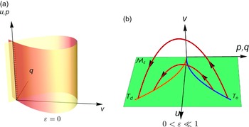
 3
3 ε=0
ε=0 Ws(Mε)
 Wu(Mε)
 0<ε≪1
0<ε≪1 Mε
Mε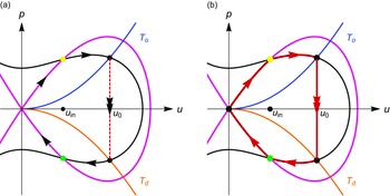
 1
1 4
4 (0,0)
(0,0) Hs(u,p)=h
 (uin,pin)
 (uout,pout)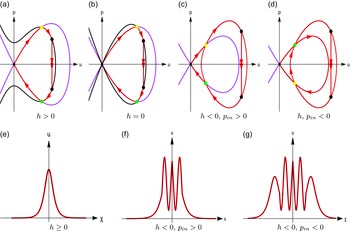
 up,0(χ)
 (u,p)
(u,p) σ>0
σ>0 u0>uin
 H=h
H=h h>0
h>0 H=h
H=h h=0
h=0 H=h
H=h h<0
h<0 pin>0
pin>0 H=h
H=h h<0
h<0 pin<0
pin<0 −
− up,0(χ)
 (χ,u)
(χ,u) ⌊LT⌋=1
 ⌊L2T⌋=1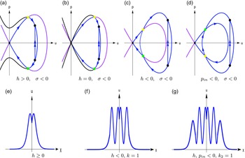
 up,0(χ)
 (u,p)
(u,p) σ<0
σ<0 u0>uin
 (χ,u)
(χ,u)
 Open access

