


1. Introduction
Nonlinearities in the equation of state for seawater density result in oceanic processes that influence the distribution of seawater in the global ocean (Nycander, Hieronymus & Roquet Reference Nycander, Hieronymus and Roquet2015). These nonlinear processes in the ocean play an important role in the climate system as they affect estimates of steric sea level change (Gille Reference Gille2004), are necessary for the formation of Antarctic intermediate water and layering of the deep waters in polar oceans (Nycander et al. Reference Nycander, Hieronymus and Roquet2015), influence the formation of sea ice (Roquet et al. Reference Roquet, Ferreira, Caneill, Schlesinger and Madec2022) and the internal pycnocline (Klocker et al. Reference Klocker, Garabato, Roquet, de Lavergne and Rintoul2023) in the Southern Ocean. Despite the known importance of nonlinear processes, quantifying their impact on other oceanic processes, such as mixing, remains a challenge.
Cabbeling and thermobaricity are the two most important nonlinear processes in the ocean (Foster Reference Foster1972; McDougall Reference McDougall1987; Nycander et al. Reference Nycander, Hieronymus and Roquet2015), with both having a significant impact on water mass transformation (Iudicone et al. Reference Iudicone, Mades, Blanke and Speich2008; Kasajima & Johannessen Reference Kasajima and Johannessen2009; Klocker & McDougall Reference Klocker and McDougall2010; Urakawa & Hasumi Reference Urakawa and Hasumi2012; Groeskamp, Abernathey & Klocker Reference Groeskamp, Abernathey and Klocker2016). Cabbeling occurs when two water parcels of equal density but differing absolute salinity (hereafter salinity or $S$
) and conservative temperature (hereafter temperature or
$S$
) and conservative temperature (hereafter temperature or $\Theta$
) are mixed to create denser water than the parent water parcels (Witte Reference Witte1902; Foster Reference Foster1972). Fofonoff (Reference Fofonoff1957) suggested that if relatively light, cold/fresh water mixes with denser warm/salty water, the gain in density from cabbeling may be sufficient for marginally stable profiles to become gravitationally unstable. This process is called cabbeling instability (Foster Reference Foster1972).
$\Theta$
) are mixed to create denser water than the parent water parcels (Witte Reference Witte1902; Foster Reference Foster1972). Fofonoff (Reference Fofonoff1957) suggested that if relatively light, cold/fresh water mixes with denser warm/salty water, the gain in density from cabbeling may be sufficient for marginally stable profiles to become gravitationally unstable. This process is called cabbeling instability (Foster Reference Foster1972).
It has been suggested that the cabbeling instability may have a strong influence on local mixing rates (Fofonoff Reference Fofonoff1957; Foster Reference Foster1972). More recently, it was suggested that cabbeling plays a significant role in shaping the thermohaline structure of high-latitude oceans (Bisits, Zika & Evans Reference Bisits, Zika and Evans2024) where conditions for cabbeling are ideal due to the relatively large temperature inversions that form between the near-freezing surface waters and deeper, denser, warmer waters. The theoretical hypothesis that cabbeling can cause convection (Fofonoff Reference Fofonoff1957), along with evidence of cabbeling’s widespread influence in the high-latitude oceans (Bisits et al. Reference Bisits, Zika and Evans2024), suggest that cabbeling may be a contributor to enhanced mixing in the high-latitude oceans. However, to date, cabbeling as a catalyst for convection has not been observed (although observing profiles that are unstable to cabbeling would be very challenging due to the short time scales over which they would be present) or simulated using turbulence-resolving simulations.
In this study, we use direct numerical simulation (DNS) to investigate the effects of cabbeling on mixing and energetic pathways. Direct numerical simulation captures processes at all scales of motion, from millimetre-scale turbulence tothe domain-scale dynamics, enabling the quantification of a closed energy budget, and accurate estimation of the sources and sinks of energy reservoirs. Direct numerical simulation has been employed to explore mixing and dissipation, for example Vreugdenhil, Gayen & Griffiths (Reference Vreugdenhil, Gayen and Griffiths2016)and Sohail et al. (Reference Sohail, Gayen and Hogg2018, Reference Sohail, Gayen and McC. Hogg2020), double diffusive effects on mixing in both the salt fingering regime, for example Shen (Reference Shen1997) and Ma & Peltier (Reference Ma and Peltier2021), and the diffusive convection regime, for example Carpenter et al. (Reference Carpenter, Sommer and Wüest2012a ,Reference Carpenter, Sommer and Wüest b ), and more recently on ocean-driven ice shelf melting (Middleton et al. Reference Middleton, Vreugdenhil, Holland and Taylor2021; Wilson et al. Reference Wilson, Vreugdenhil, Gayen and Hester2023). We use DNS in this study because cabbeling triggers mixing and flow dynamics that occur across all length scales, thus enhancing mixing rates over their molecular values. Further, DNS allows us to accurately compute how nonlinear processes influence energetics in closed systems. To our knowledge, this is the first use of DNS to explicitly simulate cabbeling, enabling a robust quantification of the impact of cabbeling on mixing rates and the energetic pathways that can form with a nonlinear equation of state.
2. Theory
2.1. Nonlinearities and mixing
Consider the hypothetical water column in figure 1(a) where there are two layers: lighter, relatively cold/fresh shallow water atop denser, warm/salty deep water. This water column is initially gravitationally stable. However, if some mixing occurs at the interface between the two layers, a spectrum of mixed water (i.e. the range of possible waters that can be formed by mixing the initial deep and shallow waters, hereafter mixed water) will form, some of which may be denser than the deeper water, thus forming an instability as in figure 1(a). Analysing the properties of the mixed water in salinity–temperature $ (S-\Theta)$
space, where these variables are conserved, illustrates how and when nonlinearities and mixing lead to cabbeling.
$ (S-\Theta)$
space, where these variables are conserved, illustrates how and when nonlinearities and mixing lead to cabbeling.
(a) Densification of mixed water at the interface of lighter cold/fresh and denser warm/salty water in a two-layer system. (b) The two-layer system in panel (a) mapped onto $S - \Theta$
space where the blue dot is the shallow cold/fresh layer and the red dot is the deeper warm/salty layer. The mixed water (purple line) crosses the isopycnal at the deep water (dotted red contour) hence an instability will form between some of the mixed water and the deep water. All figures in this study are produced using Makie.jl (Danisch & Krumbiegel Reference Danisch and Krumbiegel2021).
$S - \Theta$
space where the blue dot is the shallow cold/fresh layer and the red dot is the deeper warm/salty layer. The mixed water (purple line) crosses the isopycnal at the deep water (dotted red contour) hence an instability will form between some of the mixed water and the deep water. All figures in this study are produced using Makie.jl (Danisch & Krumbiegel Reference Danisch and Krumbiegel2021).
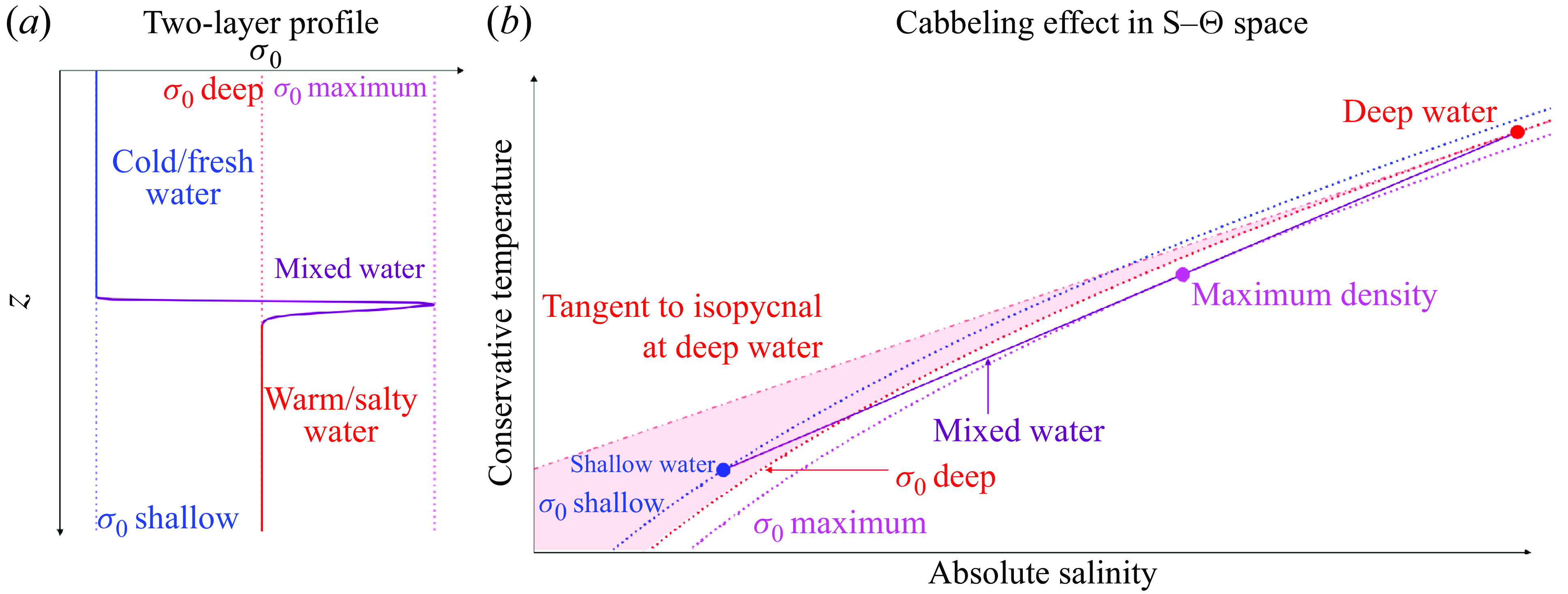
Assuming the $S-\Theta$
properties are uniform within each layer of the water column in figure 1(a), mapping the initial state of the water column into
$S-\Theta$
properties are uniform within each layer of the water column in figure 1(a), mapping the initial state of the water column into $ (S-\Theta) $
space will give just two points: the shallow cold/fresh water and the deep warm/salty water (blue and red dots respectively in figure 1
b). At constant pressure, these two water parcels are gravitationally stable as the shallower water (blue dot) is to the left of the isopycnal at the deep water (red dotted contour line) – that is,
$ (S-\Theta) $
space will give just two points: the shallow cold/fresh water and the deep warm/salty water (blue and red dots respectively in figure 1
b). At constant pressure, these two water parcels are gravitationally stable as the shallower water (blue dot) is to the left of the isopycnal at the deep water (red dotted contour line) – that is, $\rho _{{shallow}} - \rho _{{deep}} \lt 0$
.
$\rho _{{shallow}} - \rho _{{deep}} \lt 0$
.
When the shallow and deep water masses are mixed by some form of turbulent mixing, the $S-\Theta$
properties of the resulting mixtures must fall along the straight line connecting them in
$S-\Theta$
properties of the resulting mixtures must fall along the straight line connecting them in $ (S-\Theta)$
space (purple line in figure 1
b). Note that the mixture falling on a straight line is only applicable for turbulent mixing that sufficiently elevates the salinity and temperature diffusivities to an approximately homogeneous rate which temporarily overrides the transport by molecular diffusion (Guthrie, Fer & Morison Reference Guthrie, Fer and Morison2017). Due to the curvature of isopycnals, i.e. due to nonlinearity, as the water mixes, some of it becomes denser than the deep water, forming a gravitational instability between some of the mixed water and the deep water.
$ (S-\Theta)$
space (purple line in figure 1
b). Note that the mixture falling on a straight line is only applicable for turbulent mixing that sufficiently elevates the salinity and temperature diffusivities to an approximately homogeneous rate which temporarily overrides the transport by molecular diffusion (Guthrie, Fer & Morison Reference Guthrie, Fer and Morison2017). Due to the curvature of isopycnals, i.e. due to nonlinearity, as the water mixes, some of it becomes denser than the deep water, forming a gravitational instability between some of the mixed water and the deep water.
Fofonoff (Reference Fofonoff1957) hypothesised that cabbeling leads to gravitational instability when shallower waters exceed a salinity and temperature threshold set by the $S-\Theta$
properties of deeper waters. Geometrically, this threshold can be seen by considering the tangent line to the deeper water in
$S-\Theta$
properties of deeper waters. Geometrically, this threshold can be seen by considering the tangent line to the deeper water in $S-\Theta$
space (dash-dot red line in figure 1
b). Once the straight line connecting the shallow and deep waters is steeper than the tangent line to the deep water, some of the mixture must be denser than the deeper water. Thus, provided the
$S-\Theta$
space (dash-dot red line in figure 1
b). Once the straight line connecting the shallow and deep waters is steeper than the tangent line to the deep water, some of the mixture must be denser than the deeper water. Thus, provided the $S-\Theta$
properties of shallower waters are in the region between the tangent line and isopycnal to the deep water (the shaded red region in figure 1
b), cabbeling can generate a gravitational instability in a previously gravitationally stable profile. The salinity and temperature threshold from Fofonoff (Reference Fofonoff1957) can indicate when a cabbeling instability is present but gives no information about whether the instability triggers and drives further convective mixing, and if so, for how long. To quantify the effect the cabbeling instability can have on mixing we introduce a diagnostic for vertical diffusivity appropriate to DNS.
$S-\Theta$
properties of shallower waters are in the region between the tangent line and isopycnal to the deep water (the shaded red region in figure 1
b), cabbeling can generate a gravitational instability in a previously gravitationally stable profile. The salinity and temperature threshold from Fofonoff (Reference Fofonoff1957) can indicate when a cabbeling instability is present but gives no information about whether the instability triggers and drives further convective mixing, and if so, for how long. To quantify the effect the cabbeling instability can have on mixing we introduce a diagnostic for vertical diffusivity appropriate to DNS.
2.2. Effective diffusivity
Effective diffusivity is a measure of the vertical transport of a scalar field assuming the scalar field has been re-sorted so it monotonically increases with depth (Holmes et al. Reference Holmes, Zika, Griffies, Hogg, Kiss and England2021). The effective diffusivity only requires knowledge of the tracer field to compute, and is appropriate for this study as we want to diagnose cabbeling’s influence on the rate of vertical tracer transport. Diagnosing the effect cabbeling has on mixing is important for improvements to simulating convection in global ocean models.
We compute the effective diffusivity for the horizontally averaged salinity field
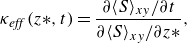 \begin{equation} \kappa _{\textit{eff}}\left (z*, t\right) = \frac {\partial \langle S \rangle _{xy}/\partial t}{\partial \langle S \rangle _{xy}/\partial z*}, \end{equation}
where the $z*$
vertical coordinate is a remapping of the horizontally averaged salinity field, indicated by
$z*$
vertical coordinate is a remapping of the horizontally averaged salinity field, indicated by $\langle \rangle _{xy}$
, into a monotonic function. In (2.1), the numerator is the vertical transport across each depth and the denominator is the vertical gradient.
$\langle \rangle _{xy}$
, into a monotonic function. In (2.1), the numerator is the vertical transport across each depth and the denominator is the vertical gradient.
The effective diffusivity can be calculated using the entire three-dimensional salinity field reshaped into a single array. However, we choose to horizontally average because initially, and towards the end of our simulations, we have two layers that are largely homogeneous leading to many instances of zero vertical gradient. Note that taking the horizontal average prior to computing the effective diffusivity is only appropriate for domains that have uniform horizontal area.
To compute (2.3) at each depth level in our domain, we first horizontally average the three-dimensional salinity field then sort from saltiest to freshest (i.e. so the saltiest water is at the bottom of the domain). Cumulatively integrating the sorted salinity array from the bottom to the top of the domain gives the horizontally averaged salinity content at each depth, the time change of which is the flux across each depth and the numerator in (2.3). Dividing the flux array element-wise by the vertical gradient of the sorted horizontally averaged salinity field, gives the effective diffusivity at each depth.
2.3. Nonlinearities and the energetics of mixing
Changes in the effective diffusivity due to enhanced mixing are also reflected in the energy budget, which captures the fluxes of energy between reservoirs. Winters et al. (Reference Winters, Lombard, Riley and D’Asaro1995) proposed possible pathways of energy between different reservoirs in a density-stratified Boussinesq flow with a linear equation of state. Within a fixed volume, the integrated total potential energy
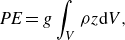 \begin{equation} \textit{PE} = g\int _{V}\rho z \mathrm{d}V, \end{equation}
can be partitioned into background potential energy, $\textit{BPE}$
, and available potential energy,
$\textit{BPE}$
, and available potential energy, $\textit{APE}$
. The
$\textit{APE}$
. The $\textit{BPE}$
is the minimum
$\textit{BPE}$
is the minimum $\textit{PE}$
state achieved by adiabatic rearrangement of fluid parcels and the
$\textit{PE}$
state achieved by adiabatic rearrangement of fluid parcels and the $\textit{APE}$
is the difference between the
$\textit{APE}$
is the difference between the $\textit{PE}$
and the
$\textit{PE}$
and the $\textit{BPE}$
. This partitioning means only
$\textit{BPE}$
. This partitioning means only $\textit{APE}$
can be converted into kinetic energy (
$\textit{APE}$
can be converted into kinetic energy ( $\textit{KE}$
), via reversible buoyancy fluxes. Changes in
$\textit{KE}$
), via reversible buoyancy fluxes. Changes in $\textit{BPE}$
are due to irreversible mixing which always acts to increase the
$\textit{BPE}$
are due to irreversible mixing which always acts to increase the $\textit{BPE}$
at the expense of the
$\textit{BPE}$
at the expense of the $\textit{APE}$
.
$\textit{APE}$
.
Urakawa, Saenz & Hogg (Reference Urakawa, Saenz and Hogg2013) showed that in a global ocean model with a nonlinear equation of state, cabbeling can be a source of $\textit{APE}$
due to isopycnal diffusion creating a reversible exchange with the
$\textit{APE}$
due to isopycnal diffusion creating a reversible exchange with the $\textit{BPE}$
reservoir. Here, we consider how cabbeling can be a source of
$\textit{BPE}$
reservoir. Here, we consider how cabbeling can be a source of $\textit{APE}$
via irreversible vertical mixing, which in current models for energetic pathways is only ever a sink for
$\textit{APE}$
via irreversible vertical mixing, which in current models for energetic pathways is only ever a sink for $\textit{APE}$
.
$\textit{APE}$
.
3. Simulations
We use DNS to explore how cabbeling can trigger and maintain convective turbulent mixing from an initially gravitationally stable state. Direct numerical simulation resolves the smallest scale at which turbulent motion occurs, typically the local Kolmogorov scale $\eta = (\nu ^{3} / \varepsilon)^{{1}/{4}}$
(where
$\eta = (\nu ^{3} / \varepsilon)^{{1}/{4}}$
(where $\nu$
is viscosity and
$\nu$
is viscosity and $\varepsilon$
is kinetic energy dissipation), and, in some cases, the local Batchelor scale. Resolving all scales of turbulence is key in this study because mixing due to cabbeling can occur at any turbulent length scale. Further, DNS allows a precise calculation of the energy budget which is crucial for understanding how nonlinear processes can drive convective mixing.
$\varepsilon$
is kinetic energy dissipation), and, in some cases, the local Batchelor scale. Resolving all scales of turbulence is key in this study because mixing due to cabbeling can occur at any turbulent length scale. Further, DNS allows a precise calculation of the energy budget which is crucial for understanding how nonlinear processes can drive convective mixing.
The DNS used in this project was built using Oceananigans.jl (Ramadhan et al. Reference Ramadhan, Wagner, Hill, Campin, Churavy, Besard, Souza, Edelman, Ferrari and Marshall2020). The DNS is non-hydrostatic and solves the incompressible Navier–Stokes equations in three dimensions under the Boussinesq approximation. The temperature and salinity tracers are set with equal, isotropic molecular diffusivity values and are evolved using the 55-term polynomial approximation to the equation of state appropriate for Boussinesq models (Roquet et al. Reference Roquet, Madec, McDougall and Barker2015). The boundary conditions for the momentum and tracers are horizontally periodic and zero-flux vertically. We set the kinematic viscosity $\nu = 1 \times 10^{-6}\,{\mathrm{m}^2 \,\mathrm{s}^{-1}}$
, and equal diffusivity values for the salt and temperature tracers
$\nu = 1 \times 10^{-6}\,{\mathrm{m}^2 \,\mathrm{s}^{-1}}$
, and equal diffusivity values for the salt and temperature tracers $\kappa = 1 \times 10^{-7}\,{\mathrm{m}^2\, \mathrm{s}^{-1}}$
resulting in a Prandtl number,
$\kappa = 1 \times 10^{-7}\,{\mathrm{m}^2\, \mathrm{s}^{-1}}$
resulting in a Prandtl number, $\mathrm{Pr} = \nu / \kappa$
, of 10. With a Prandtl number greater than one, the Batchelor scale
$\mathrm{Pr} = \nu / \kappa$
, of 10. With a Prandtl number greater than one, the Batchelor scale $\mathrm{Ba} = \eta / \sqrt {\mathrm{Pr}}$
must also be resolved in the simulations. The domain’s extent is
$\mathrm{Ba} = \eta / \sqrt {\mathrm{Pr}}$
must also be resolved in the simulations. The domain’s extent is $ [L_{x},\ L_{y},\ L_{z} ] = [{0.07}\,{\mathrm{m}},\ {0.07}\,{\mathrm{m}},\ {1}\,{\mathrm{m}} ]$
so that
$ [L_{x},\ L_{y},\ L_{z} ] = [{0.07}\,{\mathrm{m}},\ {0.07}\,{\mathrm{m}},\ {1}\,{\mathrm{m}} ]$
so that $x \in [-0.035, 0.035)$
,
$x \in [-0.035, 0.035)$
, $y \in [-0.035, 0.035)$
and
$y \in [-0.035, 0.035)$
and $z \in [-1, 0]$
. We choose a vertical extent for our domain which minimises the impact of thermobaricity (as thermobaricity only becomes significant at greater depths), thereby enabling an assessment of cabbeling instability in isolation (Harcourt Reference Harcourt2005).
$z \in [-1, 0]$
. We choose a vertical extent for our domain which minimises the impact of thermobaricity (as thermobaricity only becomes significant at greater depths), thereby enabling an assessment of cabbeling instability in isolation (Harcourt Reference Harcourt2005).
The resolution for the different experiments is set depending on the local length scale of the turbulence that is being resolved – see table 1 for the Kolmogorov and Batchelor scales, as well as the resolution set, in our simulations. The standard convergence criterion for DNS solutions requires a closed energy budget and fully resolved Kolmogorov and Batchelor scales (Gayen, Griffiths & Hughes Reference Gayen, Griffiths and Hughes2014). Our simulations meet this convergence criterion except for experiment V during $t = {6}\, \textrm{min}$
to
$t = {6}\, \textrm{min}$
to $t = {17}\,\textrm{min}$
where the local space-time minimum Batchelor length is slightly under resolved. For more details regarding the resolution set to resolve the Batchelor scale, and the energy budgets, please see Appendix A.
$t = {17}\,\textrm{min}$
where the local space-time minimum Batchelor length is slightly under resolved. For more details regarding the resolution set to resolve the Batchelor scale, and the energy budgets, please see Appendix A.
Initial $S-\Theta$
properties for the shallow water and the initial density difference between the shallow and deep water,
$S-\Theta$
properties for the shallow water and the initial density difference between the shallow and deep water, $\Delta \rho = \rho _{{shallow}} - \rho _{{deep}}$
, in all experiments. The minimum space-time local Kolmogorov (
$\Delta \rho = \rho _{{shallow}} - \rho _{{deep}}$
, in all experiments. The minimum space-time local Kolmogorov ( $\eta$
) and Batchelor (Ba) scales during the experiments and the resolution
$\eta$
) and Batchelor (Ba) scales during the experiments and the resolution $[N_{x}, N_{y}, N_{z}]$
set to resolve these scales. Initial non-dimensional numbers shown are the diffusive density ratio,
$[N_{x}, N_{y}, N_{z}]$
set to resolve these scales. Initial non-dimensional numbers shown are the diffusive density ratio, $R_{\rho }$
, the salinity Rayleigh number,
$R_{\rho }$
, the salinity Rayleigh number, $Ra_{S}$
, and the temperature Rayleigh number,
$Ra_{S}$
, and the temperature Rayleigh number, $Ra_{\Theta }$
.
$Ra_{\Theta }$
.

Although double diffusive effects have been shown to be important in a two-layer gravitationally stable system with cold/fresh water atop warm/salty water, e.g Carpenter et al. (Reference Carpenter, Sommer and Wüest2012a), we are specifically interested in the influence of nonlinear processes on turbulent vertical mixing. To allow us to focus on the effect of nonlinearities, we set the same diffusivity value (the thermal molecular diffusivity) for the salinity and temperature tracers thereby removing double diffusive effects from this study. Alternatively, we could opt to set an enhanced, equal turbulent diffusivity for both salinity and temperature, however, choosing the thermal molecular diffusivity eliminates the uncertainty involved in selecting an appropriate turbulent diffusivity, which is highly variable throughout the high-latitude oceans (e.g. Rippeth et al. (Reference Rippeth, Lincoln, Lenn, Green, Sundfjord and Bacon2015) for the Arctic Ocean). Further, we would also miss out on capturing scales of motion down to the molecular level if not resolving down to the molecular value for temperature.
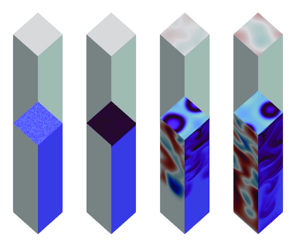
Snapshots of the flow evolution in the experiment IV. Potential density is shown on the $x{-}z$
face (at
$x{-}z$
face (at $y = -0.035$
) and the horizontal plane in the middle of the domain. Vertical velocity is shown on the
$y = -0.035$
) and the horizontal plane in the middle of the domain. Vertical velocity is shown on the $y{-}z$
face (at
$y{-}z$
face (at $x = -0.035$
) with the depth-averaged vertical velocity at the top (
$x = -0.035$
) with the depth-averaged vertical velocity at the top ( $z = 0)$
of the domain.
$z = 0)$
of the domain.
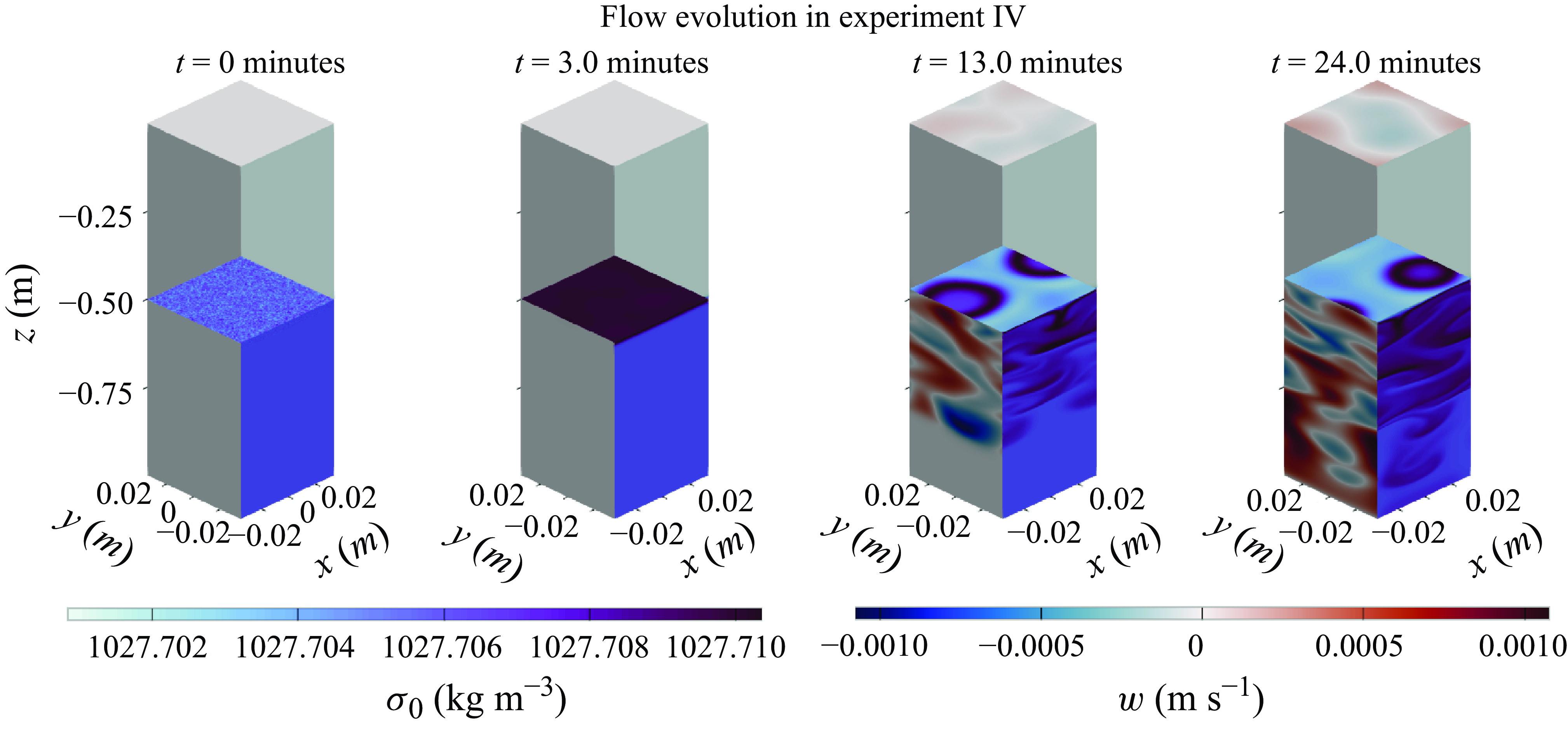
The initial state for our experiments has two layers of equal thickness. The salinity and temperature are uniform within each layer but for a small amount of noise in the salinity field about the interface, $\mathcal{O}(2 \times 10^{-4}{\mathrm{g\, kg}^{-1}})$
, seeded to kick off turbulent motion (see figure 2 at time
$\mathcal{O}(2 \times 10^{-4}{\mathrm{g\, kg}^{-1}})$
, seeded to kick off turbulent motion (see figure 2 at time $t = 0$
). Across all experiments we set the same initial salinity and temperature in the deeper layer –
$t = 0$
). Across all experiments we set the same initial salinity and temperature in the deeper layer – $S = {34.7}{\mathrm{g\, kg}}^{-1}$
and
$S = {34.7}{\mathrm{g\, kg}}^{-1}$
and $\Theta = {0.5}^{\,\circ }\textrm {C}$
. To investigate the effect of cabbeling, five experiments were run each with different
$\Theta = {0.5}^{\,\circ }\textrm {C}$
. To investigate the effect of cabbeling, five experiments were run each with different $S - \Theta$
properties in the shallower layer. The initial conditions can be seen in
$S - \Theta$
properties in the shallower layer. The initial conditions can be seen in $S - \Theta$
space in figure 3 with the values set in the shallow layer reported in table 1. Table 1 also shows relevant non-dimensional parameters for the experiments: diffusive density ratio,
$S - \Theta$
space in figure 3 with the values set in the shallow layer reported in table 1. Table 1 also shows relevant non-dimensional parameters for the experiments: diffusive density ratio, $R_{\rho }$
, salinity and temperature Rayleigh numbers,
$R_{\rho }$
, salinity and temperature Rayleigh numbers, $\mathrm{Ra}_{S} = g\beta \Delta S H^3 / \nu \kappa$
and
$\mathrm{Ra}_{S} = g\beta \Delta S H^3 / \nu \kappa$
and $\mathrm{Ra}_{\Theta } = g\alpha \Delta \Theta H^3 / \nu \kappa$
respectively. We have used equation (1) from McDougall (Reference McDougall1981) for the density ratio and the expressions for
$\mathrm{Ra}_{\Theta } = g\alpha \Delta \Theta H^3 / \nu \kappa$
respectively. We have used equation (1) from McDougall (Reference McDougall1981) for the density ratio and the expressions for $\tilde {\alpha }$
and
$\tilde {\alpha }$
and $\tilde {\beta }$
on page 93 of McDougall (Reference McDougall1981) to calculate the Rayleigh numbers. These expressions are more appropriate than evaluating
$\tilde {\beta }$
on page 93 of McDougall (Reference McDougall1981) to calculate the Rayleigh numbers. These expressions are more appropriate than evaluating $\alpha$
and
$\alpha$
and $\beta$
at midpoint salinity and temperature when the equation of state is nonlinear.
$\beta$
at midpoint salinity and temperature when the equation of state is nonlinear.
The initial salinity and temperature values used in our experiments are based on observations from the Weddell sea reported in Fofonoff (Reference Fofonoff1957). They are broadly representative of high latitude upper ocean conditions – near freezing surface water atop deeper warm salty water. The cold conditions at high latitudes are ideal for cabbeling because the dependence of density on temperature becomes increasingly nonlinear as seawater approaches its freezing point (Roquet et al. (Reference Roquet, Ferreira, Caneill, Schlesinger and Madec2022)), and temperature inversions often form between the surface and deeper waters there.
Initial conditions for the experiments run in this study in $S-\Theta$
space. The deep water properties are fixed across all experiments (red circle) and the shallow water properties (coloured markers) vary so we can determine if convection can be triggered once the system is unstable to cabbeling (i.e. once the shallow water properties lie in the wedge between the dash-dot and solid grey lines). For the
$S-\Theta$
space. The deep water properties are fixed across all experiments (red circle) and the shallow water properties (coloured markers) vary so we can determine if convection can be triggered once the system is unstable to cabbeling (i.e. once the shallow water properties lie in the wedge between the dash-dot and solid grey lines). For the $S-\Theta$
values of the shallow water see table 1.
$S-\Theta$
values of the shallow water see table 1.
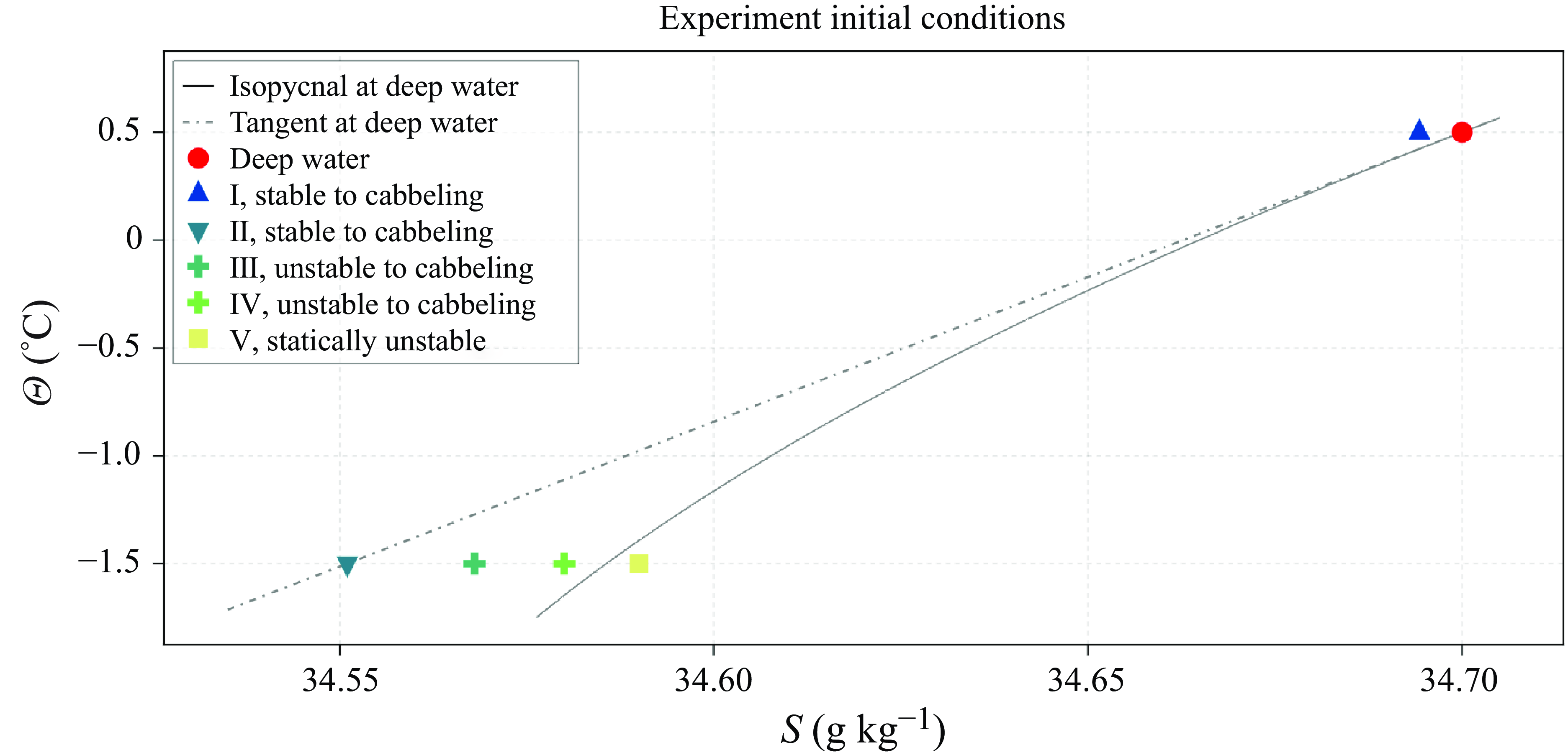
As in table 1, the initial conditions can be broken up into: statically stable, stable to cabbeling (I, II), statically stable, unstable to cabbeling (III, IV), and statically unstable (V). Experiment I has uniform temperature over the domain so that the density is only determined by the salinity scalar field. In I, a mixture of water parcels cannot exceed the maximum density of its parent waters, so we expect no instability to develop after the initial noise is dissipated. The initial conditions in experiment IV set a difference in both salinity and temperature between the two layers. Here, we expect to see a cabbeling instability develop at the interface of the two layers after a small amount of mixing has taken place. By setting the same initial density difference across the interface in experiments I and IV, we have a way of comparing the effect of cabbeling on marginally stable profiles without using a linear equation of state as this would change other aspects of the flow field.
Experiments II and III provide us with more information about when cabbeling can trigger, and its ability to sustain, an instability. Experiment II has $S-\Theta$
properties in the shallow water which place it on the theoretical limit for stability to cabbeling suggested in Fofonoff (Reference Fofonoff1957) (see figure 3). The
$S-\Theta$
properties in the shallow water which place it on the theoretical limit for stability to cabbeling suggested in Fofonoff (Reference Fofonoff1957) (see figure 3). The $S-\Theta$
properties for experiment III place it on the midpoint between the tangent and isopycnal to the deep water. Similar to IV, this initial condition is unstable to cabbeling, giving us a way to compare how convection evolves when the initial state is unstable to cabbeling to different degrees. Experiment V is statically unstable, so we are able to compare any cabbeling driven convection to convection that is also driven by gravitational instability. Note that experiment V is also influenced by cabbeling, since, when the deep and shallow waters mix, all the mixed water is denser than both of its parent waters.
$S-\Theta$
properties for experiment III place it on the midpoint between the tangent and isopycnal to the deep water. Similar to IV, this initial condition is unstable to cabbeling, giving us a way to compare how convection evolves when the initial state is unstable to cabbeling to different degrees. Experiment V is statically unstable, so we are able to compare any cabbeling driven convection to convection that is also driven by gravitational instability. Note that experiment V is also influenced by cabbeling, since, when the deep and shallow waters mix, all the mixed water is denser than both of its parent waters.
4. Results
In experiments I and II, the initial state is stable to cabbeling, meaning that after an initial enhancement in mixing due to the random noise in the salinity field, the salinity tracer mixes at approximately its parameterised value (see figure 5
b). In experiments III and IV, the initial state is statically stable but unstable to cabbeling, leading to dense water forming at the interface after some mixing has taken place – see the snapshot at $t = {3}\,\mathrm{min}$
from experiment IV in figure 2. This instability then develops and begins to drive turbulent motion that eventually is present in the entire bottom layer (see the water column at times
$t = {3}\,\mathrm{min}$
from experiment IV in figure 2. This instability then develops and begins to drive turbulent motion that eventually is present in the entire bottom layer (see the water column at times $t = {13}\,\mathrm{min}$
and
$t = {13}\,\mathrm{min}$
and $t = {24}\,\mathrm{min}$
in figure 2). Experiment V is statically unstable so we see convection immediately driven by the presence of a gravitational instability (again see figure 5
b).
$t = {24}\,\mathrm{min}$
in figure 2). Experiment V is statically unstable so we see convection immediately driven by the presence of a gravitational instability (again see figure 5
b).
4.1. Density evolution
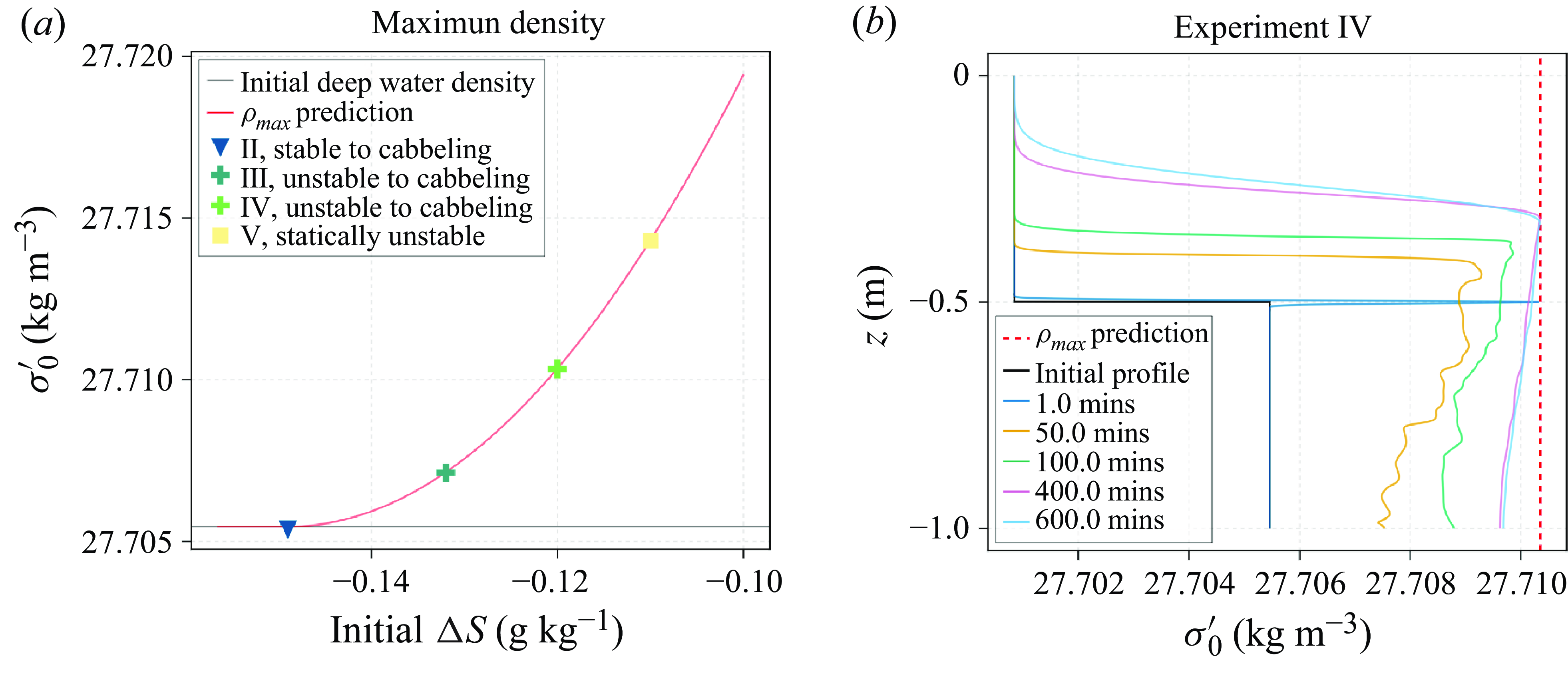
For cabbeling to form an instability from an initially gravitationally stable state, the maximum density of the mixed water, $\rho _{{max}} = \max \{\rho _{{mixed\ water}}\}$
, must be denser than the deep water
$\rho _{{max}} = \max \{\rho _{{mixed\ water}}\}$
, must be denser than the deep water
 \begin{equation} \rho _{{max}} - \rho _{{deep}} \gt 0. \end{equation}
In our closed system, the density of the mixed water is constrained to a maximum along the straight line connecting the shallow and deep waters in $(S-\Theta)$
space – an example of this is the magenta dot in figure 1
b. Hence,
$(S-\Theta)$
space – an example of this is the magenta dot in figure 1
b. Hence, $\rho _{{max}}$
will be a linear combination of the initial salinity and temperature values
$\rho _{{max}}$
will be a linear combination of the initial salinity and temperature values
 \begin{equation} \rho _{{max}} = \max \{\rho \left (S_{{deep}}+a\Delta S, \Theta _{{deep}}+a\Delta \Theta, p_0\right) : a \in [0,1]\}, \end{equation}
where $\Delta S=(S_{{shallow}} - S_{{deep}})$
,
$\Delta S=(S_{{shallow}} - S_{{deep}})$
, $\Delta \Theta =(\Theta _{{shallow}} -\Theta _{{deep}})$
,
$\Delta \Theta =(\Theta _{{shallow}} -\Theta _{{deep}})$
, $p_0$
is a reference pressure, taken to be 0 dbar in our case, and
$p_0$
is a reference pressure, taken to be 0 dbar in our case, and $a$
is a parameter indicating the relative proportion of shallow and deep waters in a given mixture. We estimate (4.2) by computing the density along the straight line connecting the initial salinity and temperature of the two layers and taking the maximum.
$a$
is a parameter indicating the relative proportion of shallow and deep waters in a given mixture. We estimate (4.2) by computing the density along the straight line connecting the initial salinity and temperature of the two layers and taking the maximum.
Figure 4(a) shows the theoretical maximum density (red curve) along with the density attained at the interface at the first saved snapshot, $t = {1}\,\mathrm{min}$
, for experiments II–V (coloured markers). We calculate (4.2) with
$t = {1}\,\mathrm{min}$
, for experiments II–V (coloured markers). We calculate (4.2) with $S_{{deep}} = {34.7}{\mathrm{g\, kg}^{-1}}$
,
$S_{{deep}} = {34.7}{\mathrm{g\, kg}^{-1}}$
, $\Theta _{{deep}} = {0.5}^{\,\circ }\textrm {C}$
,
$\Theta _{{deep}} = {0.5}^{\,\circ }\textrm {C}$
, $\Delta \Theta = -2$
, as we have in experiments II–V, over a range of values for
$\Delta \Theta = -2$
, as we have in experiments II–V, over a range of values for $\Delta S$
with
$\Delta S$
with $p_{0} = 0$
. Note we have not included experiment I because it has a different
$p_{0} = 0$
. Note we have not included experiment I because it has a different $\Delta \Theta$
. We clearly see that (4.2) is a very accurate prediction for the maximum density that is attained due to cabbeling in our experiments. Further, in experiment II, which is stable to cabbeling, we see that the maximum density does not exceed the deep water density whilst in experiments III and IV, which are statically stable but unstable to cabbeling, the maximum density is greater than the initial deep water density. This supports the hypothesis from Fofonoff (Reference Fofonoff1957) for the onset of convection due to cabbeling and suggests that while the system is unstable to cabbeling, mixing at the interface of the shallow and deep water will transform water to the theorised maximum density to sustain convection. Eventually, in a closed system, the majority of deep water, with the requisite amount of shallow water, will be brought to the maximum density at which point the system will be stable to cabbeling.
$\Delta \Theta$
. We clearly see that (4.2) is a very accurate prediction for the maximum density that is attained due to cabbeling in our experiments. Further, in experiment II, which is stable to cabbeling, we see that the maximum density does not exceed the deep water density whilst in experiments III and IV, which are statically stable but unstable to cabbeling, the maximum density is greater than the initial deep water density. This supports the hypothesis from Fofonoff (Reference Fofonoff1957) for the onset of convection due to cabbeling and suggests that while the system is unstable to cabbeling, mixing at the interface of the shallow and deep water will transform water to the theorised maximum density to sustain convection. Eventually, in a closed system, the majority of deep water, with the requisite amount of shallow water, will be brought to the maximum density at which point the system will be stable to cabbeling.
To investigate the density evolution, figure 4(b) shows horizontally averaged density profiles at various times during experiment IV, and (4.2). The profile at $t = {1}\,\mathrm{min}$
, shows mixing has caused the density at the interface to attain the density maximum. As the simulation runs, the cabbeling instability drives rapid mixing at the migrating interface, transforming the mixture of shallow and deep water to the density maximum. There also appears to be a regime shift at
$t = {1}\,\mathrm{min}$
, shows mixing has caused the density at the interface to attain the density maximum. As the simulation runs, the cabbeling instability drives rapid mixing at the migrating interface, transforming the mixture of shallow and deep water to the density maximum. There also appears to be a regime shift at $t = {400}\,\mathrm{min}$
, where even though not all the deep water has been transformed to the maximum density, the nature of the mixing at the interface appears to be more diffuse than convection-driven, indicating the system is now stable to cabbeling.
$t = {400}\,\mathrm{min}$
, where even though not all the deep water has been transformed to the maximum density, the nature of the mixing at the interface appears to be more diffuse than convection-driven, indicating the system is now stable to cabbeling.
(a) Mixed water density at the model interface at $t = {1}\,\mathrm{min}$
for experiments II–V (coloured markers) and theoretical maximum density (red line) calculated using (4.2). Experiments II–V have the same initial
$t = {1}\,\mathrm{min}$
for experiments II–V (coloured markers) and theoretical maximum density (red line) calculated using (4.2). Experiments II–V have the same initial $S_{{deep}}$
,
$S_{{deep}}$
, $\Theta _{{deep}}$
and
$\Theta _{{deep}}$
and $\Delta \Theta$
, so here
$\Delta \Theta$
, so here $\rho _{{max}}$
becomes a function of the initial
$\rho _{{max}}$
becomes a function of the initial $\Delta S$
. (b) Horizontally averaged density profiles during experiment IV with the theoretical maximum density for this experiment. In both panels the potential density is presented as an anomaly from
$\Delta S$
. (b) Horizontally averaged density profiles during experiment IV with the theoretical maximum density for this experiment. In both panels the potential density is presented as an anomaly from ${1000}\,{\mathrm{kg\, m}^{-3}}$
, i.e.
${1000}\,{\mathrm{kg\, m}^{-3}}$
, i.e. $\sigma _{0}^{\prime} = \sigma _{0} - 1000$
.
$\sigma _{0}^{\prime} = \sigma _{0} - 1000$
.
4.2. Effective diffusivity
To further investigate the apparent regime shift from cabbeling-driven convection to diffusion, we compute the effective diffusivity for the salinity tracer in all experiments using (2.1). Figure 5(a) shows the horizontally averaged effective diffusivity at each depth for experiment IV. The cabbeling instability sustains high diffusivity in much of the deeper layer until $t \approx {200}\,\mathrm{min}$
. The diffusivity in the deeper layer then begins to decrease until
$t \approx {200}\,\mathrm{min}$
. The diffusivity in the deeper layer then begins to decrease until $t \approx {400}\,\mathrm{min}$
after which point cabbeling instabilities appear to be mixed away supporting what we inferred from the density evolution in this experiment (figure 4
b). Note, the high diffusivity at the very beginning of the simulation at the top and bottom of the domain in figure 5(a) is the initial salinity noise being mixed away in the sorted horizontally averaged salinity profile.
$t \approx {400}\,\mathrm{min}$
after which point cabbeling instabilities appear to be mixed away supporting what we inferred from the density evolution in this experiment (figure 4
b). Note, the high diffusivity at the very beginning of the simulation at the top and bottom of the domain in figure 5(a) is the initial salinity noise being mixed away in the sorted horizontally averaged salinity profile.
(a) Effective diffusivity for the horizontally averaged salinity field, calculated using (2.1), for experiment IV. (b) Depth-averaged effective diffusivity for the horizontally averaged salinity field from all experiments.
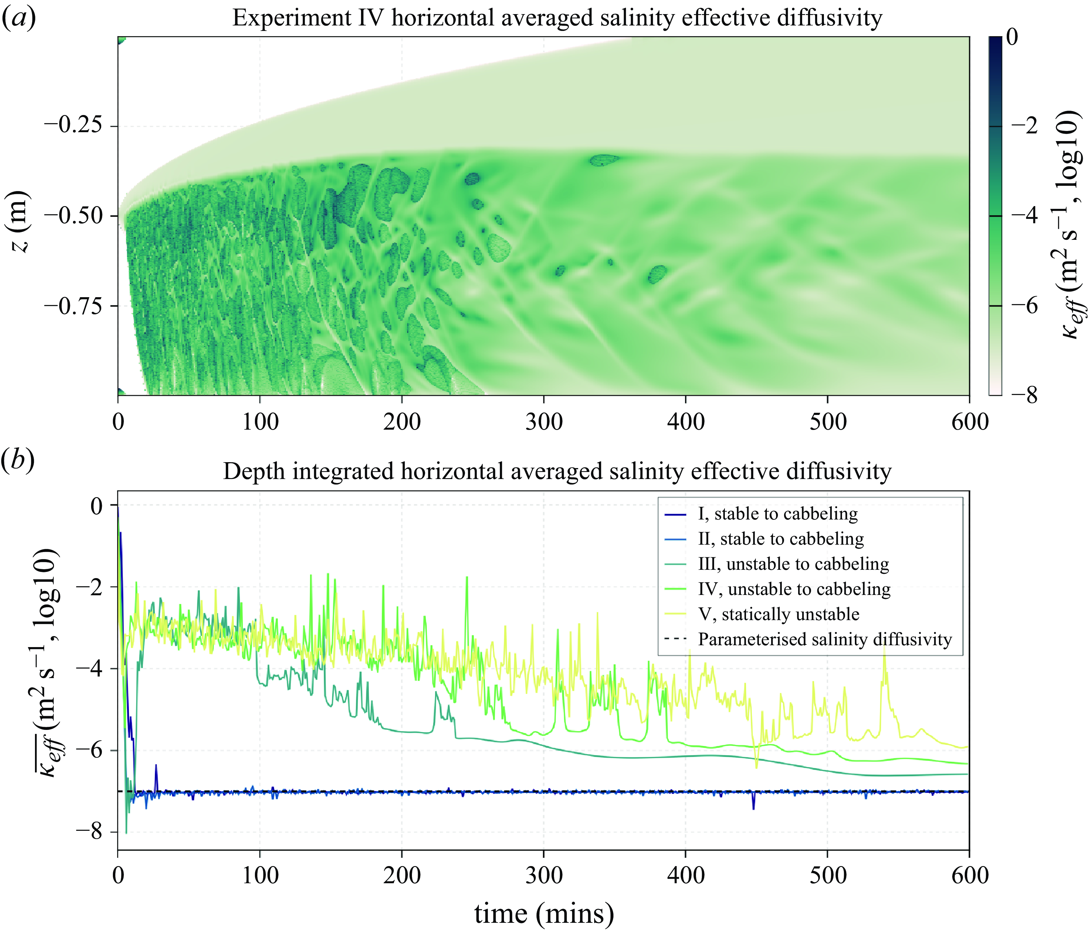
Until approximately $t = {100}\,\mathrm{min}$
in experiment III and
$t = {100}\,\mathrm{min}$
in experiment III and $t = {200}\,\mathrm{min}$
in experiment IV, cabbeling driven convection leads to an average effective diffusivity of
$t = {200}\,\mathrm{min}$
in experiment IV, cabbeling driven convection leads to an average effective diffusivity of $\overline {\kappa _{\textit{eff}}} \approx 1 \times 10^{-3}\,{\mathrm{m}^2 \,\mathrm{s}^{-1}}$
, two orders of magnitude greater than the value thought to characterise the global-averaged diapycnal diffusivity above
$\overline {\kappa _{\textit{eff}}} \approx 1 \times 10^{-3}\,{\mathrm{m}^2 \,\mathrm{s}^{-1}}$
, two orders of magnitude greater than the value thought to characterise the global-averaged diapycnal diffusivity above ${1000}\,{\mathrm{m}}$
(Waterhouse et al. Reference Waterhouse2014) and similar in magnitude to experiment V which is statically unstable (see figure 5
b). This suggests that being more unstable to cabbeling leads to longer periods of cabbeling driven convection rather than higher diffusivity. After
${1000}\,{\mathrm{m}}$
(Waterhouse et al. Reference Waterhouse2014) and similar in magnitude to experiment V which is statically unstable (see figure 5
b). This suggests that being more unstable to cabbeling leads to longer periods of cabbeling driven convection rather than higher diffusivity. After $t \approx {300}\,\mathrm{min}$
in experiment III and
$t \approx {300}\,\mathrm{min}$
in experiment III and $t \approx {400}\,\mathrm{min}$
in experiment IV the average effective diffusivity in the system decreases to approximately
$t \approx {400}\,\mathrm{min}$
in experiment IV the average effective diffusivity in the system decreases to approximately $5 \times 10^{-7}\,{\mathrm{m}^2 \,\mathrm{s}^{-1}}$
. This is still five times greater than the parameterised salinity diffusivity,
$5 \times 10^{-7}\,{\mathrm{m}^2 \,\mathrm{s}^{-1}}$
. This is still five times greater than the parameterised salinity diffusivity, $\kappa _{S} = 1 \times 10^{-7}\,{\mathrm{m}^2 \,\mathrm{s}^{-1}}$
, and experiments I and II that are stable to cabbeling where
$\kappa _{S} = 1 \times 10^{-7}\,{\mathrm{m}^2 \,\mathrm{s}^{-1}}$
, and experiments I and II that are stable to cabbeling where $\overline {\kappa _{\textit{eff}}} \approx 1 \times 10^{-7}\,{\mathrm{m}^2 \,\mathrm{s}^{-1}}$
, but is an indication that the cabbeling instability is having a reduced impact on mixing.
$\overline {\kappa _{\textit{eff}}} \approx 1 \times 10^{-7}\,{\mathrm{m}^2 \,\mathrm{s}^{-1}}$
, but is an indication that the cabbeling instability is having a reduced impact on mixing.
4.3. Energetics
The turbulent mixing we see in the simulations requires a source of $\textit{KE}$
. In our closed, initially gravitationally stable system, the
$\textit{KE}$
. In our closed, initially gravitationally stable system, the $\textit{APE}$
reservoir is the only possible source of
$\textit{APE}$
reservoir is the only possible source of $\textit{KE}$
. To track the effect cabbeling has on the
$\textit{KE}$
. To track the effect cabbeling has on the $\textit{APE}$
, we compute the
$\textit{APE}$
, we compute the $\textit{PE}$
using (2.2) and determine the
$\textit{PE}$
using (2.2) and determine the $\textit{BPE}$
as in Carpenter et al. (Reference Carpenter, Sommer and Wüest2012a
) by reshaping and sorting the three-dimensional potential density field (referenced to 0 dbar) into a monotonically increasing array and defining a height coordinate which has the same number of elements as the sorted array over the vertical extent of our domain. Again, due to the depth range we are focusing on, the thermobaric effect is negligible. The
$\textit{BPE}$
as in Carpenter et al. (Reference Carpenter, Sommer and Wüest2012a
) by reshaping and sorting the three-dimensional potential density field (referenced to 0 dbar) into a monotonically increasing array and defining a height coordinate which has the same number of elements as the sorted array over the vertical extent of our domain. Again, due to the depth range we are focusing on, the thermobaric effect is negligible. The $\textit{PE}$
and
$\textit{PE}$
and $\textit{BPE}$
are then referenced to the initial
$\textit{BPE}$
are then referenced to the initial $\textit{PE}$
,
$\textit{PE}$
, $\textit{PE}_{t = 0}$
, and non-dimensionalised so
$\textit{PE}_{t = 0}$
, and non-dimensionalised so
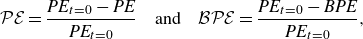 \begin{equation} \mathcal{PE} = \frac {\textit{PE}_{t = 0} - \textit{PE}}{\textit{PE}_{t = 0}} \quad \mathrm{and} \quad \mathcal{BPE} = \frac {\textit{PE}_{t = 0} - \textit{BPE}}{\textit{PE}_{t = 0}}, \end{equation}
with $\mathcal{APE} = \mathcal{PE} - \mathcal{BPE}$
.
$\mathcal{APE} = \mathcal{PE} - \mathcal{BPE}$
.
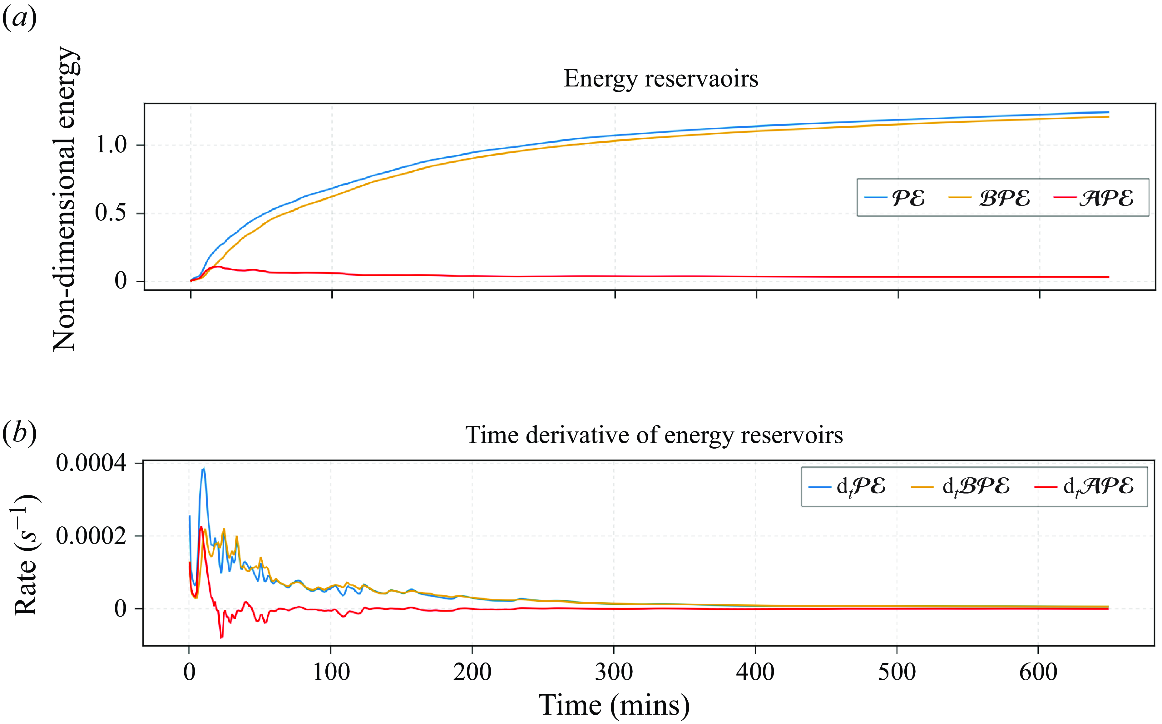
Figure 6(a) shows the time series of the $\mathcal{PE}$
,
$\mathcal{PE}$
, $\mathcal{BPE}$
and
$\mathcal{BPE}$
and $\mathcal{APE}$
during experiment IV. We see an increase in
$\mathcal{APE}$
during experiment IV. We see an increase in $\mathcal{APE}$
(red curve in figure 6
a) at the beginning of the simulation due to cabbeling forming denser waters. Figure 6(b) shows the time derivative of the energy reservoirs throughout experiment IV. The positive sign of the
$\mathcal{APE}$
(red curve in figure 6
a) at the beginning of the simulation due to cabbeling forming denser waters. Figure 6(b) shows the time derivative of the energy reservoirs throughout experiment IV. The positive sign of the $\mathcal{APE}$
time derivative (red curve in figure 6
b) indicates generation of
$\mathcal{APE}$
time derivative (red curve in figure 6
b) indicates generation of $\mathcal{APE}$
. In the time period
$\mathcal{APE}$
. In the time period $0\ \mathrm{to}\approx {20}\,\mathrm{min}$
we see the most rapid increase in
$0\ \mathrm{to}\approx {20}\,\mathrm{min}$
we see the most rapid increase in $\mathcal{APE}$
and this is purely due to cabbeling forming denser water. The cabbeling generated
$\mathcal{APE}$
and this is purely due to cabbeling forming denser water. The cabbeling generated $\mathcal{APE}$
is then lost to the
$\mathcal{APE}$
is then lost to the $\mathcal{KE}$
and
$\mathcal{KE}$
and $\mathcal{BPE}$
reservoirs from
$\mathcal{BPE}$
reservoirs from $t \approx {20}\,\mathrm{min}$
onward with intermittent production of
$t \approx {20}\,\mathrm{min}$
onward with intermittent production of $\mathcal{APE}$
as the simulation runs. The time derivative of the
$\mathcal{APE}$
as the simulation runs. The time derivative of the $\mathcal{APE}$
only becomes strictly decreasing after
$\mathcal{APE}$
only becomes strictly decreasing after $t = {602}\,\mathrm{min}$
indicating there is still
$t = {602}\,\mathrm{min}$
indicating there is still $\mathcal{APE}$
production from cabbeling till this point. However,
$\mathcal{APE}$
production from cabbeling till this point. However, $\mathcal{APE}$
production reduces after
$\mathcal{APE}$
production reduces after $t = {200}\,\mathrm{min}$
.
$t = {200}\,\mathrm{min}$
.
(a) Non-dimensional $\textit{PE}$
,
$\textit{PE}$
, $\textit{BPE}$
and
$\textit{BPE}$
and $\textit{APE}$
energy reservoirs during experiment IV. (b) The time derivative of the non-dimensional energy reservoirs throughout experiment IV.
$\textit{APE}$
energy reservoirs during experiment IV. (b) The time derivative of the non-dimensional energy reservoirs throughout experiment IV.
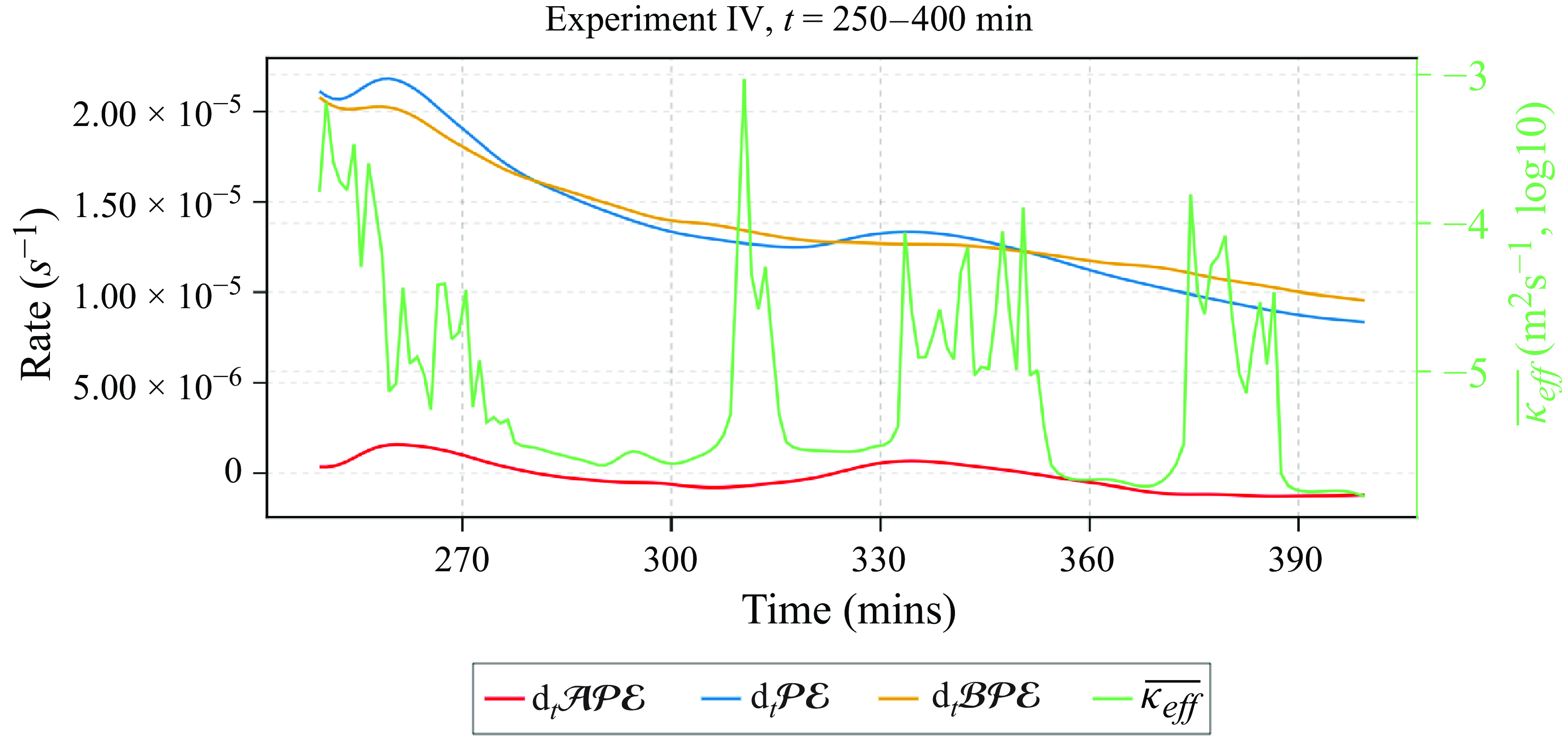
The production of $\mathcal{APE}$
is reflected in the effective diffusivity for this experiment – rapid convective mixing triggered and sustained by cabbeling producing
$\mathcal{APE}$
is reflected in the effective diffusivity for this experiment – rapid convective mixing triggered and sustained by cabbeling producing $\mathcal{APE}$
(until approximately
$\mathcal{APE}$
(until approximately $t = {200}\,\mathrm{min}$
) after which we see a decreasing trend in the effective diffusivity explained by cabbeling no longer producing
$t = {200}\,\mathrm{min}$
) after which we see a decreasing trend in the effective diffusivity explained by cabbeling no longer producing $\mathcal{APE}$
to sustain further convection. Exceptions to this trend are the three spikes in
$\mathcal{APE}$
to sustain further convection. Exceptions to this trend are the three spikes in $\overline {\kappa _{\textit{eff}}}$
between
$\overline {\kappa _{\textit{eff}}}$
between $t = {300}\,\textrm{min}\, {\textrm {to}}\,{400}\,\textrm{min}$
(see figure 5
b). The time derivative of the energy reservoirs and
$t = {300}\,\textrm{min}\, {\textrm {to}}\,{400}\,\textrm{min}$
(see figure 5
b). The time derivative of the energy reservoirs and $\overline {\kappa _{\textit{eff}}}$
during
$\overline {\kappa _{\textit{eff}}}$
during $t = {250}\,\textrm{min}\,{\textrm {to}}\,{400}\,\textrm{min}$
from experiment IV are shown in figure 7. In figure 7, we see that during
$t = {250}\,\textrm{min}\,{\textrm {to}}\,{400}\,\textrm{min}$
from experiment IV are shown in figure 7. In figure 7, we see that during $t \approx {260}\,\textrm{min}\,\text{to}\,\,{300}\,\textrm{min}$
there is a production of
$t \approx {260}\,\textrm{min}\,\text{to}\,\,{300}\,\textrm{min}$
there is a production of $\mathcal{APE}$
. By the time of the first spike in
$\mathcal{APE}$
. By the time of the first spike in $\overline {\kappa _{\textit{eff}}}$
(at
$\overline {\kappa _{\textit{eff}}}$
(at $t \approx {310}\,\mathrm{min}$
) the
$t \approx {310}\,\mathrm{min}$
) the $\mathcal{APE}$
is again decreasing suggesting some of the
$\mathcal{APE}$
is again decreasing suggesting some of the $\mathcal{APE}$
produced during
$\mathcal{APE}$
produced during $t \approx {260}\,\textrm{min}\,\textrm{to}\,\,{300}\,\textrm{min}$
has been transferred to the
$t \approx {260}\,\textrm{min}\,\textrm{to}\,\,{300}\,\textrm{min}$
has been transferred to the $\mathcal{KE}$
reservoir leading to the spike in
$\mathcal{KE}$
reservoir leading to the spike in $\overline {\kappa _{\textit{eff}}}$
. After this first spike in
$\overline {\kappa _{\textit{eff}}}$
. After this first spike in $\overline {\kappa _{\textit{eff}}}$
, we again see the production of
$\overline {\kappa _{\textit{eff}}}$
, we again see the production of $\mathcal{APE}$
followed by spikes in
$\mathcal{APE}$
followed by spikes in $\overline {\kappa _{\textit{eff}}}$
accompanied by a loss of
$\overline {\kappa _{\textit{eff}}}$
accompanied by a loss of $\mathcal{APE}$
. This suggests cabbeling is contributing to the spikes in
$\mathcal{APE}$
. This suggests cabbeling is contributing to the spikes in $\overline {\kappa _{\textit{eff}}}$
during
$\overline {\kappa _{\textit{eff}}}$
during $t = {300}\,\textrm{min}\,\textrm{to}\,{400}\,\textrm{min}$
by producing
$t = {300}\,\textrm{min}\,\textrm{to}\,{400}\,\textrm{min}$
by producing $\mathcal{APE}$
some of which is converted to
$\mathcal{APE}$
some of which is converted to $\mathcal{KE}$
.
$\mathcal{KE}$
.
Time derivative of the energy reservoirs and $\overline {\kappa _{\textit{eff}}}$
during
$\overline {\kappa _{\textit{eff}}}$
during $t = {250}\,\textrm{min}\,\text{to}\,{400}\,\textrm{min}$
from experiment IV. The left y-axis is the rate of changes in the non-dimensional energy reservoirs and the right y-axis is
$t = {250}\,\textrm{min}\,\text{to}\,{400}\,\textrm{min}$
from experiment IV. The left y-axis is the rate of changes in the non-dimensional energy reservoirs and the right y-axis is $\overline {\kappa _{\textit{eff}}}$
.
$\overline {\kappa _{\textit{eff}}}$
.
In experiments I and II, we found that after the initial $\mathcal{APE}$
injection (due to the random noise in the salinity field) was lost, there was no change in
$\mathcal{APE}$
injection (due to the random noise in the salinity field) was lost, there was no change in $\mathcal{APE}$
for the rest of the simulation (i.e.
$\mathcal{APE}$
for the rest of the simulation (i.e. $\mathrm{d}_{t}\mathcal{APE} = 0$
, figure not shown). This results in the salinity tracer evolving approximately at its parameterised value (purple line in figure 5
b). In experiment V, the initial state is statically unstable hence there is an initial source of
$\mathrm{d}_{t}\mathcal{APE} = 0$
, figure not shown). This results in the salinity tracer evolving approximately at its parameterised value (purple line in figure 5
b). In experiment V, the initial state is statically unstable hence there is an initial source of $\textit{APE}$
for the
$\textit{APE}$
for the $\textit{KE}$
to draw from. This results in high diffusivity occurring immediately in experiment V (see the yellow line figure 5
b). Cabbeling still has an effect in experiment V by creating denser water at the interface, thereby generating
$\textit{KE}$
to draw from. This results in high diffusivity occurring immediately in experiment V (see the yellow line figure 5
b). Cabbeling still has an effect in experiment V by creating denser water at the interface, thereby generating $\textit{APE}$
. Experiment V differs from experiments III and IV because, even though in all cases cabbeling generates
$\textit{APE}$
. Experiment V differs from experiments III and IV because, even though in all cases cabbeling generates $\textit{APE}$
through densification of the mixed water at the interface, experiments III and IV have no initial
$\textit{APE}$
through densification of the mixed water at the interface, experiments III and IV have no initial $\textit{APE}$
, therefore enhanced mixing only occurs after cabbeling has generated a sufficient amount of
$\textit{APE}$
, therefore enhanced mixing only occurs after cabbeling has generated a sufficient amount of $\textit{APE}$
.
$\textit{APE}$
.
5. Discussion
Our results demonstrate that cabbeling can trigger and sustain convection in profiles that are initially gravitationally stable. Whilst a cabbeling instability is present in our initially gravitationally stable experiments (III and IV) we see elevated diffusivity, which is the same order of magnitude as generated by the initially gravitationally unstable profile (experiment V), alongside a production of $\textit{APE}$
.
$\textit{APE}$
.
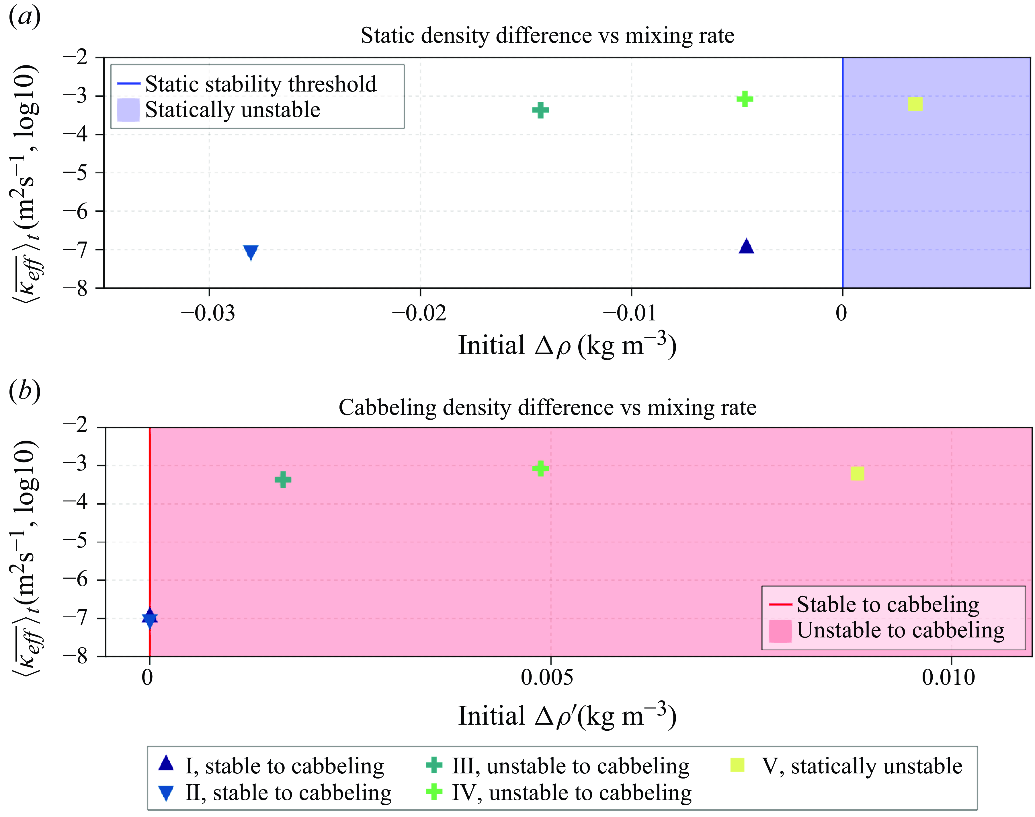
If cabbeling were having no effect in the global ocean then we would expect to see profiles approaching the static stability limit prior to the onset of convection. Instead the results of Bisits et al. (Reference Bisits, Zika and Evans2024) show the cabbeling instability threshold describes well the stability limiting behaviour of profiles in the high-latitude oceans. In figure 8(a), we see that high diffusivity can be generated and sustained from a statically stable initial state (experiments III and IV). This supports the notion of a cabbeling instability threshold by demonstrating that the initial state need not be gravitationally unstable for the onset of convection. Instead, cabbeling can cause the gravitationally stable initial state to become unstable leading to convection. Combined with the results in Bisits et al. (Reference Bisits, Zika and Evans2024), this reinforces the important role cabbeling may play in the high-latitude oceans.
The static density difference, $\Delta \rho$
, between two waters with distinct
$\Delta \rho$
, between two waters with distinct $S-\Theta$
properties cannot predict when a cabbeling instability is present in statically stable profiles. From (4.1) we can define a cabbeling density difference,
$S-\Theta$
properties cannot predict when a cabbeling instability is present in statically stable profiles. From (4.1) we can define a cabbeling density difference, $\Delta \rho ^{\prime} = \rho _{{max}} - \rho _{{deep}}$
, such that
$\Delta \rho ^{\prime} = \rho _{{max}} - \rho _{{deep}}$
, such that
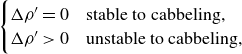 \begin{equation} \begin{cases} \Delta \rho ^{\prime} = 0 \quad \text{stable to cabbeling,} \\ \Delta \rho ^{\prime} \gt 0 \quad \text{unstable to cabbeling,} \end{cases} \end{equation}
providing a binary distinction for the cabbeling instability. Panel (b) in figure 8 shows the time mean effective diffusivity for salinity, $\langle \overline {\kappa _{\textit{eff}}}\rangle _{t}$
, during
$\langle \overline {\kappa _{\textit{eff}}}\rangle _{t}$
, during $t = {11}\,\textrm{min}\,\textrm{to}\,{300}\,\textrm{min}$
against the initial cabbeling density difference for all experiments. We see that that the stable to cabbeling experiments (I and II) have
$t = {11}\,\textrm{min}\,\textrm{to}\,{300}\,\textrm{min}$
against the initial cabbeling density difference for all experiments. We see that that the stable to cabbeling experiments (I and II) have $\Delta \rho ^{\prime} = 0$
, hence no instability can form from cabbeling. As a result we see no enhancement of
$\Delta \rho ^{\prime} = 0$
, hence no instability can form from cabbeling. As a result we see no enhancement of $\overline {\kappa _{\textit{eff}}}$
. The statically stable, unstable to cabbeling experiments (III and IV) have
$\overline {\kappa _{\textit{eff}}}$
. The statically stable, unstable to cabbeling experiments (III and IV) have $\Delta \rho ^{\prime} \gt 0$
and we see that elevated diffusivity is sustained in the time period
$\Delta \rho ^{\prime} \gt 0$
and we see that elevated diffusivity is sustained in the time period $t = {11}\,\textrm{min}\,\textrm{to}\,{300}\,\textrm{min}$
in those experiments. Using (5.1) for investigating the stability of profiles to cabbeling may yield further insight into the role of cabbeling in the global ocean.
$t = {11}\,\textrm{min}\,\textrm{to}\,{300}\,\textrm{min}$
in those experiments. Using (5.1) for investigating the stability of profiles to cabbeling may yield further insight into the role of cabbeling in the global ocean.
(a) Time average, indicated by $\langle \rangle _{t}$
, of effective diffusivity (
$\langle \rangle _{t}$
, of effective diffusivity ( $\overline {\kappa _{\textit{eff}}}$
) during
$\overline {\kappa _{\textit{eff}}}$
) during $t = {11}\,\textrm{min}\,\textrm{to}\,{300}\,\textrm{min}$
of the experiments. Here, the x-axis is
$t = {11}\,\textrm{min}\,\textrm{to}\,{300}\,\textrm{min}$
of the experiments. Here, the x-axis is $\Delta \rho = \rho _{{shallow}} - \rho _{{deep}}$
, meaning there is no indication of the profile being unstable to cabbeling. Panel (b) shows the same time average of
$\Delta \rho = \rho _{{shallow}} - \rho _{{deep}}$
, meaning there is no indication of the profile being unstable to cabbeling. Panel (b) shows the same time average of $\overline {\kappa _{\textit{eff}}}$
but this time the x-axis is
$\overline {\kappa _{\textit{eff}}}$
but this time the x-axis is $\Delta \rho ^{\prime} = \rho _{{max}} - \rho _{{deep}}$
which is a binary criteria for determining if a profile is unstable to cabbeling (equation (5.1)).
$\Delta \rho ^{\prime} = \rho _{{max}} - \rho _{{deep}}$
which is a binary criteria for determining if a profile is unstable to cabbeling (equation (5.1)).
Our results suggest that the cabbeling instability needs to be taken into account when simulating convection and included in models of energetic pathways. Typically, global ocean and coupled climate models employ convective adjustment schemes to diagnose, and instantaneously mix away gravitational instabilities. Therefore, these schemes do not take into account how a cabbeling instability can trigger and sustain convection when water columns are gravitationally stable. To accurately simulate convection in regions where the conditions for cabbeling are prime, e.g. at high latitudes, parameterisations may need to be adjusted to factor in the cabbeling instability.
Current models of energetic pathways, e.g. Winters et al. (Reference Winters, Lombard, Riley and D’Asaro1995); Hughes, Hogg & Griffiths (Reference Hughes, Hogg and Griffiths2009), define $\textit{APE}$
as gravitational potential energy relative to the lowest possible energy state under adiabatic redistribution (i.e. relative to the
$\textit{APE}$
as gravitational potential energy relative to the lowest possible energy state under adiabatic redistribution (i.e. relative to the $\textit{BPE}$
). This definition means that in a closed system, mixing can only reduce
$\textit{BPE}$
). This definition means that in a closed system, mixing can only reduce $\textit{APE}$
by transferring energy to the
$\textit{APE}$
by transferring energy to the $\textit{BPE}$
. However, our simulations demonstrate that mixing leads to a production of
$\textit{BPE}$
. However, our simulations demonstrate that mixing leads to a production of $\textit{APE}$
while a cabbeling instability is present. Adapting models of energetic pathways to account for nonlinear processes, by for example, redefining
$\textit{APE}$
while a cabbeling instability is present. Adapting models of energetic pathways to account for nonlinear processes, by for example, redefining $\textit{APE}$
or
$\textit{APE}$
or $\textit{BPE}$
, is crucial for increased understanding of the energetics of mixing in the ocean.
$\textit{BPE}$
, is crucial for increased understanding of the energetics of mixing in the ocean.
The simulations run in this study are designed to focus on cabbeling. However, there are other nonlinear and small-scale processes that impact mixing and energetics in the ocean. In particular, future work may consider understanding the impact and interplay of thermobaricity and/or double diffusive instabilities, yielding a more complete picture of fine-scale ocean mixing, energetics and dynamics. Regardless of the domain size in our experiment setup, cabbeling will lead to denser water than the deep water forming at the interface of the two layers, and enhanced mixing rates, from initial conditions that are unstable to cabbeling. That being said, changes in domain size and aspect ratio may lead to different flow structure thereby influencing our transport diagnostics, however, this is not something we investigate in this study (see Wang et al. Reference Wang, Chong, Stevens, Verzicco and Lohse2020 for how domain aspect ratio influences flow structure in Rayleigh Bernard convection).
6. Conclusion
In this work, we have simulated convection triggered by density production due to cabbeling in a direct numerical simulation for the first time. We have demonstrated the impact of this ‘cabbeling instability’ on gravitationally stable vertical profiles. We show the significant influence cabbeling has on mixing rates and the energetics of mixing, and discuss the implications of these findings on global ocean modelling and observations.
In our cabbeling experiments, after an initial perturbation, mixing is enhanced until the fluid reaches a state where cabbeling can no longer destabilise the water column – that is, until the system becomes stable to cabbeling. This means the majority of the deep water in the two-layer system transforms to a predicted maximum density. We find that densification from cabbeling creates a source of gravitational $\textit{APE}$
which drives turbulent motion and generation of
$\textit{APE}$
which drives turbulent motion and generation of $\textit{KE}$
without any external forcing and continues to do so until the system is stable to cabbeling. This suggests either an exception to the rule that mixing always decreases the APE in a closed system, or that the definition of
$\textit{KE}$
without any external forcing and continues to do so until the system is stable to cabbeling. This suggests either an exception to the rule that mixing always decreases the APE in a closed system, or that the definition of $\textit{APE}$
or
$\textit{APE}$
or $\textit{BPE}$
should be modified to account for nonlinear changes in density with mixing. These results highlight the importance of the cabbeling instability in both high-latitude ocean modelling and mixing, and emphasise the need to reconsider energy budgets to account for the influence of cabbeling instability on energy reservoirs.
$\textit{BPE}$
should be modified to account for nonlinear changes in density with mixing. These results highlight the importance of the cabbeling instability in both high-latitude ocean modelling and mixing, and emphasise the need to reconsider energy budgets to account for the influence of cabbeling instability on energy reservoirs.
Acknowledgements.
This research was undertaken with the assistance of resources from the National Computational Infrastructure (NCI Australia), an NCRIS enabled capability supported by the Australian Government. We also wish to thank B. Gayen, T. McDougall and I. Conde for their discussions and insights during the course of this study. We also wish to thank three anonymous reviewers whose feedback significantly improved this study.
Funding.
The authors acknowledge support from the Australian Research Council, grant number SR200100008 (J.I.B., T.S. and J.D.Z.). This research has been supported by an Australian Government Research Training Program (RTP) Scholarship (J.I.B.).
Declaration of interests.
The authors report no conflict of interest.
Data availability statement.
The code used to produce all model output, analysis and figures in this study can be found in the public code repository https://github.com/jbisits/CabbelingExperiments. Analysis data files used to produce the figures can be found at doi: 10.6084/m9.figshare.28012616
Appendix A.
In table 1, we report the minimum space–time value for the local Batchelor length $(\mathrm{Ba})$
during each experiment. Provided our grid resolution is less than the minimum Batchelor length (i.e.
$(\mathrm{Ba})$
during each experiment. Provided our grid resolution is less than the minimum Batchelor length (i.e. $\Delta x \lt \mathrm{Ba}$
,
$\Delta x \lt \mathrm{Ba}$
, $\Delta y \lt \mathrm{Ba}$
and
$\Delta y \lt \mathrm{Ba}$
and $\Delta z \lt \mathrm{Ba}$
) the experiment will resolve the Batchelor scale at all points in space and time.
$\Delta z \lt \mathrm{Ba}$
) the experiment will resolve the Batchelor scale at all points in space and time.
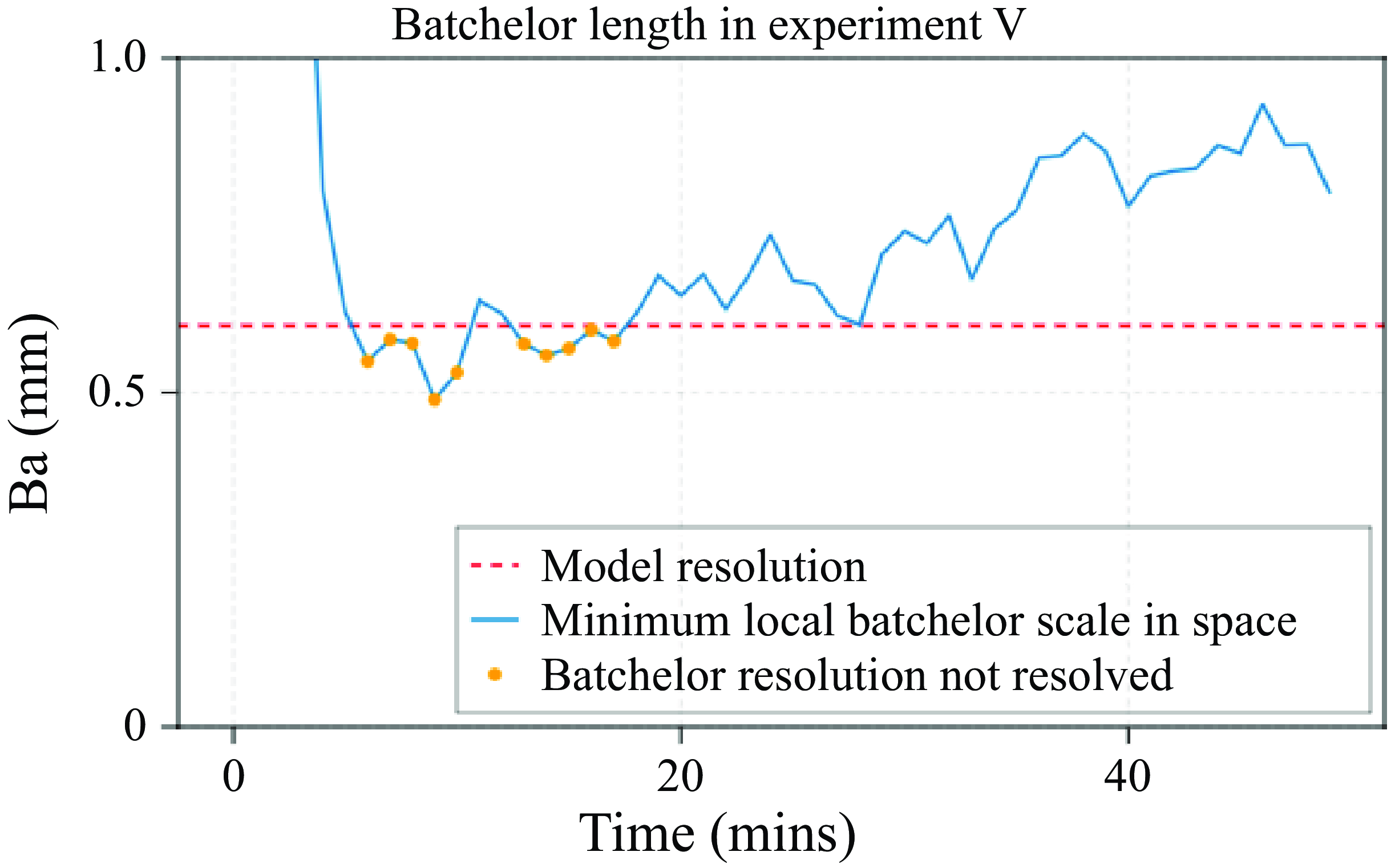
The horizontal and vertical resolution in experiment I is 2 mm with a Batchelor length of 13.83 mm giving us sufficient resolution to resolve the Batchelor scale at all points in space and time in experiment I. The horizontal and vertical resolution in experiments II–V is 0.6 mm. For experiments II–IV this again gives us sufficient resolution to resolve the local Batchelor scale at all points in space and time (see table 1 for the Batchelor length in these experiments). In experiment V we find the minimum local Batchelor scale is not resolved between $t = {6}\, \textrm {min}\,\textrm{to} \,{10}\, \textrm {min}$
and
$t = {6}\, \textrm {min}\,\textrm{to} \,{10}\, \textrm {min}$
and $t = {13}\, \textrm{min}\, \textrm {to}\,{17}\, \textrm{min}$
(see figure 9). We still have a closed energy budget (see below), so results from
$t = {13}\, \textrm{min}\, \textrm {to}\,{17}\, \textrm{min}$
(see figure 9). We still have a closed energy budget (see below), so results from $t = {6}\, \textrm{min}\, \textrm {to}\, {17}\, \textrm{min}$
are reported with confidence that the DNS solution converges even though we are slightly under resolving the Batchelor scale during this time.
$t = {6}\, \textrm{min}\, \textrm {to}\, {17}\, \textrm{min}$
are reported with confidence that the DNS solution converges even though we are slightly under resolving the Batchelor scale during this time.
Time series of the minimum local Batchelor scale in experiment V for the first 50 min. The orange dots indicate the saved snapshots where the local minimum Batchelor scale is not resolved.
To achieve a closed energy budget in our DNS experiments we require the production and dissipation of kinetic energy to balance (Gayen et al. Reference Gayen, Griffiths and Hughes2014). Within our closed system, changes in the volume integrated $(\textit{KE})$
reservoir are due to turbulent kinetic energy dissipation,
$(\textit{KE})$
reservoir are due to turbulent kinetic energy dissipation, $\varepsilon$
, and the volume integrated buoyancy flux (which is the production of
$\varepsilon$
, and the volume integrated buoyancy flux (which is the production of $\textit{KE}$
). Therefore, to achieve a closed energy budget we require
$\textit{KE}$
). Therefore, to achieve a closed energy budget we require
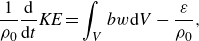 \begin{equation} \frac {1}{\rho _{0}}\frac {\mathrm{d}}{\mathrm{d}t}\textit{KE} = \int _{V}bw\mathrm{d}V -\frac {\varepsilon }{\rho _{0}}, \end{equation}
where $\rho _{0}$
is the reference density used in the simulations. To determine if (A1) is satisfied, we compute each term in (A1) individually. Figure 10 shows that, qualitatively the energy budget is balanced for all experiments. The titles in each panel also report the mean absolute error (MAE) between the left- and right-hand sides of (A1),
$\rho _{0}$
is the reference density used in the simulations. To determine if (A1) is satisfied, we compute each term in (A1) individually. Figure 10 shows that, qualitatively the energy budget is balanced for all experiments. The titles in each panel also report the mean absolute error (MAE) between the left- and right-hand sides of (A1),
 \begin{equation} \mathrm{MAE} = \left \langle \left |\frac {1}{\rho _{0}}\frac {\mathrm{d}}{\mathrm{d}t}\textit{KE} - \left (\int _{V}bw\mathrm{d}V -\frac {\varepsilon }{\rho _{0}}\right)\right |\right \rangle _{t}. \end{equation}
The closure of our energy budget and resolution sufficient to resolve the Batchelor scale, show how we satisfy the standard convergence criteria for DNS solutions (Gayen et al. Reference Gayen, Griffiths and Hughes2014).


 Open access