



1. Introduction
The interaction between dispersed particles and rotor flows represents a fundamental problem in fluid mechanics, central to applications ranging from energy conversion to atmospheric and environmental processes. From turbomachinery and propulsion devices to energy systems, rotors frequently operate in conditions where a dispersed phase interacts with the surrounding air. Examples include aircraft propellers, helicopter rotors and wind turbines, as well as industrial fans and cooling towers. Such interactions are now encountered even in extraterrestrial atmospheres: between 2021 and 2024, the Ingenuity Mars Helicopter (Balaram, Aung & Golombek Reference Balaram, Aung and Golombek2021) completed 72 flights in the dusty environment of Mars, marking a new era of planetary exploration. In all these contexts, suspended solid or liquid particles interact with the rotor blades and the induced flow field, whether intentionally or incidentally, making it essential to understand the underlying particle–flow dynamics.
Two illustrative examples of rotor–particle interaction are ice accretion and particle-induced erosion on rotor blades. These opposing yet physically related processes are governed by the interaction of particles with a solid surface, one leading to material accumulation and the other to material removal, mainly on the leading edge of the blade. Ice accretion occurs when supercooled water droplets impact a surface, breaking their unstable equilibrium and solidifying on the blade (Guardone et al. Reference Guardone, Bellosta, Donizetti and Gallia2026). It occurs over a time frame ranging from minutes to hours, depending on rotor size and operating conditions, and the consequences span from aerodynamic degradation to safety hazards. In a longer time frame, the impact of sand and rain on blades may lead to leading-edge erosion, causing a permanent degradation of blade aerodynamics; interestingly, the study of drop impact dynamics originated to understand rain-induced erosion (Cheng, Sun & Gordillo Reference Cheng, Sun and Gordillo2022). The problems are shared among rotors of different sizes and purposes, ranging from microscale propellers to helicopter and large wind turbine rotors.
The investigation of such problems on rotors has been pursued extensively through both experimental and numerical means. Special attention has been devoted to ice accretion due to its inherent safety risks. In the case of propellers, their relatively small size allows for full scale or quasi-full scale experimental testing in icing wind tunnels, as demonstrated in several campaigns (e.g. by Karli, Yan & Palacios (Reference Karli, Yan and Palacios2024) and Yan et al. (Reference Yan, Nangle, Karli and Palacios2024), Hardenberg, Flack & Rigby (Reference Hardenberg, Flack and Rigby2024) and Müller & Hann (Reference Müller and Hann2022)). Conversely, icing experiments on full-scale helicopters (Shaw & Ritcher Reference Shaw and Ritcher1985) are generally limited to natural icing conditions due to the constraints imposed by rotor size and test facility capabilities. Wind tunnel experiments are typically conducted on scaled models under controlled conditions (Britton, Bond & Flemming Reference Britton, Bond and Flemming1994; Kind et al. Reference Kind, Potapczuk, Feo, Golia and Shah1998). For wind turbines, experimental studies involving multiphase flow are commonly restricted to scaled fixed (Hochart et al. Reference Hochart, Fortin, Perron and Ilinca2008) or rotating (Han, Palacios & Schmitz Reference Han, Palacios and Schmitz2012) sectional models due to the large scale of the system.
In the past, full three-dimensional (3-D) numerical simulations remained limited due to a combination of the lack of computational tools and high computational cost. Recent advancements in software development and high-performance computing have enabled the development of high-fidelity numerical approaches that offer a cost-effective and safer alternative to in-flight testing. Yet, reduced-order models based on isolated two-dimensional (2-D) blade sections, originally developed for helicopter icing (Gent & Cansdale Reference Gent and Cansdale1985), are still widely used in various modified forms, to reduce computational time, explore broader design spaces (Gallia, Caccia & Guardone Reference Gallia, Caccia and Guardone2024) and complex events (Switchenko et al. Reference Switchenko, Habashi, Reid, Ozcer and Baruzzi2014), or introduce relevant physics such as blade plunging and pitching motions (Narducci, Orr & Kreeger Reference Narducci, Orr and Kreeger2012; Kelly et al. Reference Kelly, Habashi, Quaranta, Masarati and Fossati2018; Min & Yee Reference Min and Yee2023) and the history of the angle of attack of a blade section operating in a turbulent boundary layer (Gimenez, Idelsohn & Oñate Reference Gimenez, Idelsohn and Oñate2024; Tahani, Hossein & Hong Reference Tahani, Hossein and Hong2024).
In 2-D approximations, the sectional flow field is generally computed considering the local angle of attack of the section, i.e. the angle between the local chord and the vector resulting from the composition of the free stream wind vector, the induced velocity vector and the local section velocity, projected in the section plane. The angle is either chosen to be representative of normal operating conditions or estimated with some inexpensive aerodynamic model, e.g. the blade element momentum theory (BEMT). At times, the induced velocity vector is even neglected for convenience (Heramarwan et al. Reference Heramarwan, Müller, Hann and Lutz2023). The dispersed phase is then solved considering a one-way coupling and initial equilibrium with the flow field. The approach is shared for studying both ice accretion (Martini et al. Reference Martini, Ilinca, Rizk, Ibrahim and Issa2022; Caccia & Guardone Reference Caccia and Guardone2023; Caccia, Abergo & Guardone Reference Caccia, Abergo and Guardone2024) and erosion (Castorrini et al. Reference Castorrini, Corsini, Rispoli, Venturini, Takizawa and Tezduyar2019).
To introduce the focus of this work, it is useful to analyse the works by Fiore and Selig for damage and erosion of wind turbine sections. In Fiore & Selig (Reference Fiore and Selig2015), they investigated sand and insect damage considering the standard workflow described earlier, i.e. computing the sectional flow field at standard operating angles of attack and presumably introducing the dispersed phase in equilibrium with the section velocity vector. Later, Fiore, Fujiwara & Selig (Reference Fiore, Fujiwara and Selig2016) investigated rain and hailstone damage in similar sectional conditions. Since heavy particles were considered, these were injected in the sectional flow field with their terminal velocity as seen by the section, i.e. in non-equilibrium with the free stream flow field seen by the section, which includes the induced velocity.
Let us provide a visual representation of the problem in figure 1. The diagrams illustrate the behaviour of two particles of different sizes as they approach a wind turbine blade section. The section is located at a distance $r$
from the rotation axis as highlighted in figure 1(a), together with the free stream velocity vector
$r$
from the rotation axis as highlighted in figure 1(a), together with the free stream velocity vector $\boldsymbol V_\infty$
, the rotation speed
$\boldsymbol V_\infty$
, the rotation speed $\varOmega$
and the tangential velocity
$\varOmega$
and the tangential velocity $\varOmega r$
. We start considering a 3-D description of the problem in figure 1(b). The velocity triangle of the carrying phase results from the sum of
$\varOmega r$
. We start considering a 3-D description of the problem in figure 1(b). The velocity triangle of the carrying phase results from the sum of $V_\infty$
with the axial induced velocity
$V_\infty$
with the axial induced velocity $aV_\infty$
(where
$aV_\infty$
(where $a$
is the axial induction factor) in the
$a$
is the axial induction factor) in the $x$
direction and of
$x$
direction and of $\varOmega r$
with the tangential induced velocity
$\varOmega r$
with the tangential induced velocity $a'\varOmega r$
(where
$a'\varOmega r$
(where $a'$
is the tangential induction factor) in the
$a'$
is the tangential induction factor) in the $y$
direction. On a rotor providing momentum to the surrounding fluid, the direction of the axial and tangential induced velocities would be opposite.
$y$
direction. On a rotor providing momentum to the surrounding fluid, the direction of the axial and tangential induced velocities would be opposite.
Let us now introduce particles in the flow field of figure 1(b). The behaviour of a particle in the flow field is determined by its Stokes number ${\textit{Stk}} = {\tau _p}/{\tau _{\kern-1pt f}}$
, where
${\textit{Stk}} = {\tau _p}/{\tau _{\kern-1pt f}}$
, where $\tau _p$
is the particle relaxation time and
$\tau _p$
is the particle relaxation time and $\tau _{\kern-1pt f}$
is a characteristic time scale of the carrier flow. A sufficiently small particle, i.e. a particle with
$\tau _{\kern-1pt f}$
is a characteristic time scale of the carrier flow. A sufficiently small particle, i.e. a particle with ${\textit{Stk}} \ll 1$
, will adapt almost instantly to the flow field, leading to a tracking trajectory that closely follows the streamlines of the carrying phase. Larger particles require a longer time to adapt to the flow field; thus, they deviate from it, especially in high streamline curvature regions. If a particle coming from the free stream is sufficiently large (
${\textit{Stk}} \ll 1$
, will adapt almost instantly to the flow field, leading to a tracking trajectory that closely follows the streamlines of the carrying phase. Larger particles require a longer time to adapt to the flow field; thus, they deviate from it, especially in high streamline curvature regions. If a particle coming from the free stream is sufficiently large ( ${\textit{Stk}} \gg 1$
), it is unaffected by the flow features, including the induced velocity field, and follows a ballistic trajectory.
${\textit{Stk}} \gg 1$
), it is unaffected by the flow features, including the induced velocity field, and follows a ballistic trajectory.
We then restrict the problem to an infinite wing, equivalent to a 2-D sectional description. In this case, if we prescribe the angle of attack $\alpha _{\mathit{aero}}$
obtained considering the induced velocities in the free stream conditions seen by the section (figure 1
c), the flow field close to the section will be almost equivalent to the 3-D one of figure 1(b), in the absence of relevant 3-D phenomena. Thus, a particle with
$\alpha _{\mathit{aero}}$
obtained considering the induced velocities in the free stream conditions seen by the section (figure 1
c), the flow field close to the section will be almost equivalent to the 3-D one of figure 1(b), in the absence of relevant 3-D phenomena. Thus, a particle with ${\textit{Stk}} \ll 1$
will follow the correct tracking trajectory. However, a particle with
${\textit{Stk}} \ll 1$
will follow the correct tracking trajectory. However, a particle with ${\textit{Stk}} \gg 1$
released in equilibrium at the free stream will necessarily follow a wrong ballistic trajectory, which includes the induced velocity component. We note that this is the state-of-the-art description of the sectional problem e.g. as presented by Barfknecht & von Terzi (Reference Barfknecht and von Terzi2024).
${\textit{Stk}} \gg 1$
released in equilibrium at the free stream will necessarily follow a wrong ballistic trajectory, which includes the induced velocity component. We note that this is the state-of-the-art description of the sectional problem e.g. as presented by Barfknecht & von Terzi (Reference Barfknecht and von Terzi2024).
Conversely, if we do not consider the induced velocities for the free stream conditions seen by the section (figure 1
d), we obtain a geometric angle of attack $\alpha _{\mathit{geom}}$
. In this case, neither the carrier velocity field around the section, nor the tracking trajectories (
$\alpha _{\mathit{geom}}$
. In this case, neither the carrier velocity field around the section, nor the tracking trajectories ( ${\textit{Stk}} \ll 1$
) will represent the 3-D solution. However, ballistic trajectories (
${\textit{Stk}} \ll 1$
) will represent the 3-D solution. However, ballistic trajectories ( ${\textit{Stk}} \gg 1$
) will be correct.
${\textit{Stk}} \gg 1$
) will be correct.
Representation of a tracking and a ballistic trajectory. (a) A 3-D global view of a wind turbine rotor, highlighting the plane analysed; (b) 3-D solution in a reference frame fixed with the rotor: the tracking trajectory is affected by the induced velocity, and the ballistic trajectory is not; (c) 2-D Ind sectional description: the induced velocity contributes to the free stream velocity vector; (d) 2-D Geom sectional description: the induced velocity does not contribute to the free stream velocity vector.

Figure 1. Long description
Panel A: A 3-D global view of a wind turbine rotor, highlighting the plane analyzed. The rotor includes a blade, hub, and nacelle, with an inset showing a close-up of the blade’s leading edge. Panel B: A 3-D solution in a reference frame fixed with the rotor. The tracking trajectory is affected by the induced velocity, and the ballistic trajectory is not. The diagram shows the paths of particles relative to the rotating blade. Panel C: A 2-D Ind sectional description. The induced velocity contributes to the free stream velocity vector. The diagram illustrates the interaction of particles with the blade’s leading edge, showing both ballistic and tracking trajectories. Panel D: A 2-D Geom sectional description. The induced velocity does not contribute to the free stream velocity vector. The diagram shows the paths of particles relative to the blade’s leading edge, highlighting the difference between ballistic and tracking trajectories.
This informal analysis suggests that restricting the problem to a 2-D analysis would likely result in two classes of correct solutions for the dispersed phase dynamics around the section, which depend on the Stokes number. For ${\textit{Stk}} \ll 1$
, the correct solution is obtained by matching the flow field, i.e. by using
${\textit{Stk}} \ll 1$
, the correct solution is obtained by matching the flow field, i.e. by using $\alpha _{\mathit{aero}}$
(figure 1
c). We refer to this modelling approach as 2-D Ind. For
$\alpha _{\mathit{aero}}$
(figure 1
c). We refer to this modelling approach as 2-D Ind. For ${\textit{Stk}} \gg 1$
, the correct solution is obtained by neglecting the induced velocity, i.e. by using
${\textit{Stk}} \gg 1$
, the correct solution is obtained by neglecting the induced velocity, i.e. by using $\alpha _{\mathit{geom}}$
(figure 1
d). We name this modelling approach 2-D Geom.
$\alpha _{\mathit{geom}}$
(figure 1
d). We name this modelling approach 2-D Geom.
In this work, we investigate the dynamics of heavy inertial particles impinging on rotor blades and their response to the induced velocity field through the comparison of the 3-D solution with the 2-D Ind and 2-D Geom approaches. Through this comparison, we demonstrate that these are the two limiting cases and identify the range of Stokes numbers under which they provide the correct representation of the problem. The analysis is supported by an analytical model derived to compute the delayed response of a particle to the rotor-induced velocity field, which can be used in 2-D sectional representations of the problem. The study is conducted numerically on a wind turbine rotor and a small-scale propeller in axial flow conditions, considering particle sizes relevant in real applications.
The paper is structured as follows. We start by defining the modelling assumptions and the numerical methods in § 2. In § 3 we present and discuss the results related to the 2-D limiting solutions introduced in figure 1 through the comparison with 3-D results. In § 4 we present and validate the model for computing the delayed response of a particle to the rotor-induced velocity field. In § 5, we summarise the transport regimes identified for the particles and the relationship between the observed phenomena and rotor size. Conclusions are reported in § 6.
2. Methodology
We consider water droplets dispersed in air due to their relevance in many engineering problems. This naturally bounds the study to the heavy particle limit, characterised by a particle density $\rho _p$
much greater than the carrier’s density
$\rho _p$
much greater than the carrier’s density $\rho _{\kern-1pt f}$
, namely,
$\rho _{\kern-1pt f}$
, namely, $\rho _p \gg \rho _{\kern-1pt f}$
. The analysis is carried out under the following assumptions.
$\rho _p \gg \rho _{\kern-1pt f}$
. The analysis is carried out under the following assumptions.
-
(i) The carrier phase is described by the steady Reynolds-averaged Navier–Stokes (RANS) equations. Only axial flight conditions with steady and uniform inflow velocity are considered, leading to a steady 3-D solution when computed in a rotating reference frame. Also, the gravitational force acting on the particles is neglected, as it would introduce a time-dependent solution if the force is not aligned with the rotation axis.
-
(ii) The flow is modelled under a one-way coupling assumption, and the dispersed phase is influenced by the carrier phase, but not vice versa. This assumption is justified under a low volume fraction and mass loading of the dispersed phase (Balachandar & Eaton Reference Balachandar and Eaton2010), and is standard for the class of problems considered in this study.
-
(iii) Particles stick upon impact and do not break up or rebound. Although this is an approximation for large water droplets, the assumption does not interfere with the phenomena observed in this work and allows generalisation to solid particles. Moreover, it will be possible to discuss the behaviour of secondary droplets in 2-D and 3-D simulations in view of the results obtained. Yarin (Reference Yarin2006) reviewed such particle–surface interactions in detail.
Moreover, monodispersed clouds are studied, and each particle size is characterised independently. In practical applications, particle populations are typically polydisperse and their overall behaviour can be modelled as the superposition of multiple discrete particle-diameter bins.
The solution procedure is the same for both 2-D and 3-D simulations and consists of solving the dispersed phase after the carrying phase, as detailed in the following subsections. However, 2-D simulations usually require an additional step to get the local boundary conditions on the section. Besides using generic operational angles of attack of the sections, common practices include using the BEMT to obtain the induced velocity at the blade section considering the operating conditions of the rotor, as reviewed by Martini et al. (Reference Martini, Ilinca, Rizk, Ibrahim and Issa2022) for wind turbine applications, and changing the angle of attack of the 2-D simulation to match the pressure coefficient distribution on the pressure side of the corresponding section of the 3-D rotor, as proposed by Narducci & Kreeger (Reference Narducci and Kreeger2012) and Narducci et al. (Reference Narducci, Orr and Kreeger2012) and recently applied by Oztekin & Bain (Reference Oztekin and Bain2024) on a propeller. To compute $\alpha _{\mathit{aero}}$
in the 2-D Ind case of figure 1(c), we will cover both approaches, and use the former for the wind turbine rotor and the latter for the small-scale propeller. For the 2-D Geom case of figure 1(d),
$\alpha _{\mathit{aero}}$
in the 2-D Ind case of figure 1(c), we will cover both approaches, and use the former for the wind turbine rotor and the latter for the small-scale propeller. For the 2-D Geom case of figure 1(d), $\alpha _{\mathit{geom}}$
is retrieved analytically.
$\alpha _{\mathit{geom}}$
is retrieved analytically.
2.1. Solution of the carrying phase
The flow field is computed by solving RANS equations in the open-source toolkit SU2 (Economon et al. Reference Economon, Palacios, Copeland, Lukaczyk and Alonso2015). The toolkit SU2 solves the governing equations using a node-centred finite volume method on unstructured grids. In particular, the governing equations are written with an arbitrary Lagrangian–Eulerian differential form as
 \begin{align} \frac {\partial {\boldsymbol{U}}}{\partial t} + \boldsymbol{\nabla }\boldsymbol{\cdot }\boldsymbol{{F}^c_{\textit{ALE}}} - \boldsymbol{\nabla }\boldsymbol{\cdot }\boldsymbol{F}^v - \boldsymbol{Q} = 0\, , \end{align}
where $\boldsymbol{U} = \{\rho _{\kern-1pt f},\,\rho _{\kern-1pt f} \boldsymbol{v}_{\kern-1pt f},\,\rho _{\kern-1pt f} E\}^{\text{T}}$
is the vector of conservative variables,
$\boldsymbol{U} = \{\rho _{\kern-1pt f},\,\rho _{\kern-1pt f} \boldsymbol{v}_{\kern-1pt f},\,\rho _{\kern-1pt f} E\}^{\text{T}}$
is the vector of conservative variables, $\boldsymbol{F}^c_{\textit{ALE}}$
are the convective fluxes in the arbitrary Lagrangian–Eulerian formulation,
$\boldsymbol{F}^c_{\textit{ALE}}$
are the convective fluxes in the arbitrary Lagrangian–Eulerian formulation, $ \boldsymbol{F}^v$
are the viscous fluxes and
$ \boldsymbol{F}^v$
are the viscous fluxes and $\boldsymbol{Q}$
is a generic source term;
$\boldsymbol{Q}$
is a generic source term; $\rho _{\kern-1pt f}$
is the fluid density,
$\rho _{\kern-1pt f}$
is the fluid density, $\boldsymbol{v}_{\kern-1pt f}$
is the fluid velocity in the inertial reference frame and
$\boldsymbol{v}_{\kern-1pt f}$
is the fluid velocity in the inertial reference frame and $E$
is the total energy per unit mass. The vector of convective fluxes
$E$
is the total energy per unit mass. The vector of convective fluxes $\boldsymbol{F}^c_{\textit{ALE}}$
is
$\boldsymbol{F}^c_{\textit{ALE}}$
is
 \begin{align} \boldsymbol{F}^c_{\textit{ALE}} = \begin{Bmatrix} \rho _{\kern-1pt f}(\boldsymbol{v}_{\kern-1pt f}-\boldsymbol{v}_\varOmega ) \\[4pt]\rho _{\kern-1pt f} \boldsymbol{v}_{\kern-1pt f} \otimes (\boldsymbol{v}_{\kern-1pt f}-\boldsymbol{v}_\varOmega ) + \unicode{x1D644}p \\[4pt]\rho _{\kern-1pt f} (\boldsymbol{v}_{\kern-1pt f} -\boldsymbol{v}_\varOmega )E + p\boldsymbol{v}_{\kern-1pt f} \end{Bmatrix} , \end{align}
where $\boldsymbol{v}_\varOmega$
is the velocity of the domain,
$\boldsymbol{v}_\varOmega$
is the velocity of the domain, $p$
is the static pressure and
$p$
is the static pressure and $\unicode{x1D644}$
is the identity matrix. Let us consider a reference frame rotating with velocity
$\unicode{x1D644}$
is the identity matrix. Let us consider a reference frame rotating with velocity $\boldsymbol \varOmega$
and denote with
$\boldsymbol \varOmega$
and denote with $\boldsymbol r$
the distance vector from the rotation centre. By setting
$\boldsymbol r$
the distance vector from the rotation centre. By setting $({\partial \boldsymbol{U}}/{\partial t}) = \boldsymbol 0$
,
$({\partial \boldsymbol{U}}/{\partial t}) = \boldsymbol 0$
, $\boldsymbol v_\varOmega = \boldsymbol \varOmega \times \boldsymbol r$
and
$\boldsymbol v_\varOmega = \boldsymbol \varOmega \times \boldsymbol r$
and $\boldsymbol Q = \{0, -\rho _{\kern-1pt f}(\boldsymbol \varOmega \times \boldsymbol v_{\kern-1pt f}), 0\}^{\text{T}}$
, and by providing an appropriate turbulence closure for
$\boldsymbol Q = \{0, -\rho _{\kern-1pt f}(\boldsymbol \varOmega \times \boldsymbol v_{\kern-1pt f}), 0\}^{\text{T}}$
, and by providing an appropriate turbulence closure for $\boldsymbol{F}^v$
, one obtains the steady RANS equations in a non-inertial, rotating reference frame written in the absolute velocity formulation. In the RANS framework, closure is provided by the Spalart–Allmaras turbulence model from Spalart & Allmaras (Reference Spalart and Allmaras1992), whereas we modelled laminar–turbulent transition with the algebraic BCM (Bas–Cakmakcioglu modified) model by Cakmakcioglu et al. (Reference Cakmakcioglu, Bas, Mura and Kaynak2020).
$\boldsymbol{F}^v$
, one obtains the steady RANS equations in a non-inertial, rotating reference frame written in the absolute velocity formulation. In the RANS framework, closure is provided by the Spalart–Allmaras turbulence model from Spalart & Allmaras (Reference Spalart and Allmaras1992), whereas we modelled laminar–turbulent transition with the algebraic BCM (Bas–Cakmakcioglu modified) model by Cakmakcioglu et al. (Reference Cakmakcioglu, Bas, Mura and Kaynak2020).
In 2-D, once the local boundary conditions are known and the grid is generated, the flow field is simulated on the sections chosen for the analysis. We discretised the convective fluxes with the Roe scheme, using a MUSCL (monotonic upstream-centered scheme for conservation laws) scheme for flux reconstruction to recover second-order accuracy in space. Convergence was obtained after the reduction of the root mean square of the residual on the density by six orders of magnitude and the satisfaction of a Cauchy criterion for lift and drag over the last 200 iterations with a threshold value of $10^{-6}$
. In three dimensions, the convective fluxes are discretised using the Jameson–Schmidt–Turkel scheme. Convergence is checked both on the root mean square of the residual of the density, where we aim at a reduction by four orders of magnitude and on the stabilisation of rotor thrust and torque with a Cauchy criterion as for the 2-D simulations. In both cases, the convective term of the turbulence transport equation is discretised with a first-order scalar upwind scheme. A free stream turbulence intensity of 0.2 % was considered.
$10^{-6}$
. In three dimensions, the convective fluxes are discretised using the Jameson–Schmidt–Turkel scheme. Convergence is checked both on the root mean square of the residual of the density, where we aim at a reduction by four orders of magnitude and on the stabilisation of rotor thrust and torque with a Cauchy criterion as for the 2-D simulations. In both cases, the convective term of the turbulence transport equation is discretised with a first-order scalar upwind scheme. A free stream turbulence intensity of 0.2 % was considered.
2.2. Solution of the dispersed phase
We use a discrete parcel method to track the position of computational parcels in the flow field, using the in-house Lagrangian particle tracking code PoliDrop (Bellosta et al. Reference Bellosta, Baldan, Sirianni and Guardone2023). The trajectory of a particle of mass $m_p$
, diameter
$m_p$
, diameter $d_p$
and moving with velocity
$d_p$
and moving with velocity $\boldsymbol v_p$
is computed by integrating in time
$\boldsymbol v_p$
is computed by integrating in time $t$
the following differential equation, where the only external force is the aerodynamic drag as heavy particles are considered (
$t$
the following differential equation, where the only external force is the aerodynamic drag as heavy particles are considered ( $\rho _p \gg \rho _{\kern-1pt f}$
):
$\rho _p \gg \rho _{\kern-1pt f}$
):
 \begin{align} \frac {\partial \boldsymbol v_p}{\partial t} = \frac {1}{m_p}\frac {\pi }{8}\,(\boldsymbol v_{\kern-1pt f} - \boldsymbol v_p)\,\mu _{\kern-1pt f}\,d_p\, \textit{Re}_p\,C_{D,p}\, , \end{align}
where $\mu _{\kern-1pt f}$
is the carrier phase dynamic viscosity, whereas
$\mu _{\kern-1pt f}$
is the carrier phase dynamic viscosity, whereas $ \textit{Re}_p$
and
$ \textit{Re}_p$
and $C_{D,p}$
are the particle’s Reynolds number and drag coefficient, respectively. The former is defined as
$C_{D,p}$
are the particle’s Reynolds number and drag coefficient, respectively. The former is defined as
 \begin{align} \textit{Re}_p = \frac {\rho _{\kern-1pt f}\,||\boldsymbol v_{\kern-1pt f}-\boldsymbol v_p||_2\,d_p}{\mu _{\kern-1pt f}}. \end{align}
The drag coefficient of the droplet accounts for its deformation from a perfect sphere to an oblate disk due to the aerodynamic forces. It is expressed as a combination of the drag of a sphere $C_{D,\textit{sphere}}$
and that of a disk
$C_{D,\textit{sphere}}$
and that of a disk $C_{D,\textit{disk}}$
weighted on the eccentricity
$C_{D,\textit{disk}}$
weighted on the eccentricity $\varepsilon$
and it is defined as
$\varepsilon$
and it is defined as
 \begin{align} C_{D,p}= \begin{cases} (1-\varepsilon )\,C_{D,\textit{sphere}} + \varepsilon \,C_{D, \textit{disk}} & \text{if }\textit {We}_p \le 12\\[4pt] C_{D, \textit{disk}} & \text{if }\textit {We}_p \gt 12 \end{cases} \end{align}
where $\varepsilon = (1+0.07\sqrt {\textit {We}_p} )^{-6}$
depends on the Weber number of the particle
$\varepsilon = (1+0.07\sqrt {\textit {We}_p} )^{-6}$
depends on the Weber number of the particle $\textit {We}_p=\rho _p||\boldsymbol v_{\kern-1pt f}-\boldsymbol v_p||^2d_p/\sigma _p$
, which expresses the ratio between inertia and surface tension forces;
$\textit {We}_p=\rho _p||\boldsymbol v_{\kern-1pt f}-\boldsymbol v_p||^2d_p/\sigma _p$
, which expresses the ratio between inertia and surface tension forces; $\sigma _p$
is the droplet surface tension. For more details, the reader is referred to Bellosta et al. (Reference Bellosta, Baldan, Sirianni and Guardone2023), where the routines for parcel localisation and the solution interpolation are verified and the code is validated against experimental measurements on fixed wings.
$\sigma _p$
is the droplet surface tension. For more details, the reader is referred to Bellosta et al. (Reference Bellosta, Baldan, Sirianni and Guardone2023), where the routines for parcel localisation and the solution interpolation are verified and the code is validated against experimental measurements on fixed wings.
A single, straight (2-D) or planar (3-D), uniform front of droplets is released in local equilibrium with the unperturbed flow. In three dimensions, the dispersed phase is tracked in a rotating reference frame using an algorithm that avoids integrating the non-inertial accelerations, thus eliminating the discretisation error related to their integration, as detailed in Caccia & Guardone (Reference Caccia and Guardone2025). After the particles’ impact, an automatic cloud adaptation strategy is deployed to refine the initial cloud front and iteratively obtain a converged solution. The simulation is considered converged when the $\ell ^2$
norm of the difference of the collection efficiency in two consecutive iterations is below a specified threshold. The threshold is set to
$\ell ^2$
norm of the difference of the collection efficiency in two consecutive iterations is below a specified threshold. The threshold is set to $10^{-6}$
and
$10^{-6}$
and $2\times 10^{-3}$
for 2-D and 3-D simulations, respectively.
$2\times 10^{-3}$
for 2-D and 3-D simulations, respectively.
2.3. Collection efficiency
A fundamental metric for characterising multiphase rotor dynamics is the fraction of the dispersed phase free stream mass flux impacting at a given location on the blade surface. Depending on the application, it is referred to by various names, including collection efficiency, collision efficiency, impingement efficiency and hit rate. In this work, we adopt the term collection efficiency and denote it by the symbol $\beta$
. Numerically, the collection efficiency
$\beta$
. Numerically, the collection efficiency $\beta _i$
on the cell
$\beta _i$
on the cell $i$
of the boundary is computed as
$i$
of the boundary is computed as
 \begin{align} \beta _i = \frac {\mathop\sum \limits_{j\in i} m_{p,j} \phi _j}{A_i \rho ^*_c}\, , \end{align}
where $A_i$
is the area of the cell at impact,
$A_i$
is the area of the cell at impact, $\rho ^*_c$
is the computational cloud density computed as the ratio between the total cloud mass and the area of the injection front and
$\rho ^*_c$
is the computational cloud density computed as the ratio between the total cloud mass and the area of the injection front and $m_{\kern-1pt j}$
is the mass of the jth particle impinging on cell
$m_{\kern-1pt j}$
is the mass of the jth particle impinging on cell $i$
. Here
$i$
. Here $\phi _j$
is a flux coefficient to account for the orientation of the cloud front at the free stream with respect to the relative velocity
$\phi _j$
is a flux coefficient to account for the orientation of the cloud front at the free stream with respect to the relative velocity
 \begin{align} \phi _j = \frac {\boldsymbol V_{\kern-1.5pt \mathit{fs}} - \boldsymbol \varOmega \times \boldsymbol r_{0p,j}}{V_{\mathit{fs}}} \boldsymbol{\cdot }\, \hat {\boldsymbol n}_c, \end{align}
where $\hat {\boldsymbol n}_c$
is the unit vector normal to the seeding plane and
$\hat {\boldsymbol n}_c$
is the unit vector normal to the seeding plane and $\boldsymbol r_{0p,j}$
is the jth particle distance vector from the rotation axis at the release location;
$\boldsymbol r_{0p,j}$
is the jth particle distance vector from the rotation axis at the release location; $\boldsymbol V_{\kern-1.5pt \mathit{fs}}$
represents the free stream velocity vector and
$\boldsymbol V_{\kern-1.5pt \mathit{fs}}$
represents the free stream velocity vector and $V_{\mathit{fs}}=||\boldsymbol{V}_{\mathit{fs}}||_2$
(this convention will be used from now on). In three dimensions,
$V_{\mathit{fs}}=||\boldsymbol{V}_{\mathit{fs}}||_2$
(this convention will be used from now on). In three dimensions, $\boldsymbol V_{\kern-1.5pt \mathit{fs}}=\boldsymbol V_\infty$
; in two dimensions,
$\boldsymbol V_{\kern-1.5pt \mathit{fs}}=\boldsymbol V_\infty$
; in two dimensions, $\boldsymbol V_{\kern-1.5pt \mathit{fs}}$
is the free stream velocity vector as seen by the section. This allows results independent of the orientation of the seeding plane in both the inertial and rotating reference frames. Then, the mass per unit time impinging on the cell can be computed as
$\boldsymbol V_{\kern-1.5pt \mathit{fs}}$
is the free stream velocity vector as seen by the section. This allows results independent of the orientation of the seeding plane in both the inertial and rotating reference frames. Then, the mass per unit time impinging on the cell can be computed as
 \begin{align} \dot {m_i} = \rho _c\, V_{\mathit{fs}} \,A_i\,\beta _i, \end{align}
where $\rho _c$
is the cloud density indicating the mass of dispersed phase contained in a unit volume of the carrying phase. In the case of water droplets,
$\rho _c$
is the cloud density indicating the mass of dispersed phase contained in a unit volume of the carrying phase. In the case of water droplets, $\rho _c$
is generally named liquid water content. Finally, the local volumetric flux
$\rho _c$
is generally named liquid water content. Finally, the local volumetric flux $\dot {\mu }$
and a section-normalised collection efficiency
$\dot {\mu }$
and a section-normalised collection efficiency $\hat {\beta }$
are computed as
$\hat {\beta }$
are computed as
 \begin{align} \dot {\mu }_i = \frac {\dot {m}_i}{\rho _c}\frac {1}{A_i} \end{align}
and
 \begin{align} \hat {\beta }_i = \frac {\dot {\mu }_i}{||{\boldsymbol V_{\kern-1.5pt \mathit{fs}} - \boldsymbol \varOmega \times \boldsymbol r_i}||_2}\, , \end{align}
where $\boldsymbol r_i$
is the distance vector of the cell from the rotation centre. In three dimensions, the first quantity shows the variation of impinging particle volume along the blade span, while the second provides a comparison with the fixed-wing equivalent collection efficiency. In two dimensions,
$\boldsymbol r_i$
is the distance vector of the cell from the rotation centre. In three dimensions, the first quantity shows the variation of impinging particle volume along the blade span, while the second provides a comparison with the fixed-wing equivalent collection efficiency. In two dimensions, $\hat \beta _i=\beta _i$
, and
$\hat \beta _i=\beta _i$
, and $\hat \beta _i$
is therefore used for comparing 2-D and 3-D simulations consistently.
$\hat \beta _i$
is therefore used for comparing 2-D and 3-D simulations consistently.
Finally, it is also possible to compute analytically the limit collection efficiency for an ideal ballistic trajectory as
 \begin{align} {\beta }_{i,\mathit{ball}} = - \frac {{\boldsymbol V_{\kern-1.5pt \mathit{fs}} - \boldsymbol \varOmega \times \boldsymbol r_i}}{V_{\mathit{fs}}} \boldsymbol{\cdot }\hat {\boldsymbol n}_i\, , \end{align}
where $\hat {\boldsymbol n}_i$
is the local surface normal vector, positive outwards; the result can be normalised according to (2.8)–(2.10). It is also necessary to set
$\hat {\boldsymbol n}_i$
is the local surface normal vector, positive outwards; the result can be normalised according to (2.8)–(2.10). It is also necessary to set ${\beta }_{i,\mathit{ball}}=0$
on surface cells that are in the shadow of other cells, i.e. only the first crossing of the ballistic trajectory with the body should be considered; this automatically excludes any cell with
${\beta }_{i,\mathit{ball}}=0$
on surface cells that are in the shadow of other cells, i.e. only the first crossing of the ballistic trajectory with the body should be considered; this automatically excludes any cell with ${\beta }_{i,\mathit{ball}}\lt 0$
.
${\beta }_{i,\mathit{ball}}\lt 0$
.
2.4. Stokes numbers
The results are presented and discussed in terms of the Stokes number ${\textit{Stk}}={\tau _p}/{\tau _{\kern-1pt f}}$
. In the Stokesian regime, i.e. if the particle Reynolds number
${\textit{Stk}}={\tau _p}/{\tau _{\kern-1pt f}}$
. In the Stokesian regime, i.e. if the particle Reynolds number $ \textit{Re}_p\ll 1$
, the particle relaxation time is
$ \textit{Re}_p\ll 1$
, the particle relaxation time is
 \begin{align} \tau _{p,0} = \frac {\rho _p\,d_p^2}{18\,\mu _{\kern-1pt f}}. \end{align}
For non-Stokesian particles, a correction factor $\psi (\textit{Re}_p)$
is required, leading to
$\psi (\textit{Re}_p)$
is required, leading to
 \begin{align} \tau _p = \tau _{p,0}\,\psi (\textit{Re}_p), \end{align}
with
 \begin{align} \psi ( \textit{Re}_p) = \frac {24}{ \textit{Re}_p} \int _0^{ \textit{Re}_p} \frac {\text{d} \textit{Re}'}{C_D( \textit{Re}') \textit{Re}'}\, \end{align}
as first introduced by Israel & Rosner (Reference Israel and Rosner1982). Thus, it is possible to express $\textit{Stk}$
as
$\textit{Stk}$
as
 \begin{align} {\textit{Stk}} = {\textit{Stk}}_0\,\psi (\textit{Re}_p), \end{align}
where ${\textit{Stk}}_0 = \tau _{p,0}/\tau _{\kern-1pt f}$
. We will first use
${\textit{Stk}}_0 = \tau _{p,0}/\tau _{\kern-1pt f}$
. We will first use ${\textit{Stk}}_0$
to obtain a magnitude estimate for
${\textit{Stk}}_0$
to obtain a magnitude estimate for $\textit{Stk}$
; in § 4, this assumption will be removed.
$\textit{Stk}$
; in § 4, this assumption will be removed.
The fluid characteristic time can be expressed differently according to the phenomenon of interest. Depending on the choice, a definition of the Stokes number follows. Given a time-averaged solution, e.g. the output of RANS equations, the local characteristic time scale of the flow can be defined as $\tau _{f,\mathit{loc}}=1/||\boldsymbol{\nabla }\boldsymbol v_{\kern-1pt f}||_2$
(we consider the Frobenius norm). On an airfoil section, the time scale can be defined as
$\tau _{f,\mathit{loc}}=1/||\boldsymbol{\nabla }\boldsymbol v_{\kern-1pt f}||_2$
(we consider the Frobenius norm). On an airfoil section, the time scale can be defined as $\tau _{f,\textit{sec}}=c/V_{\textit{rel}}$
, where
$\tau _{f,\textit{sec}}=c/V_{\textit{rel}}$
, where $c$
is the chord of the section and
$c$
is the chord of the section and $V_{\textit{rel}}$
is the relative velocity between the section and the fluid. Also, it is possible to define a time scale
$V_{\textit{rel}}$
is the relative velocity between the section and the fluid. Also, it is possible to define a time scale $\tau _{f,\textit{ind}}$
related to the flow in the stream tube upstream of the rotor, where the induction is generated. Following these time scales, we can define a local, sectional and induction Stokes number as
$\tau _{f,\textit{ind}}$
related to the flow in the stream tube upstream of the rotor, where the induction is generated. Following these time scales, we can define a local, sectional and induction Stokes number as
 \begin{align} {\textit{Stk}}_{\mathit{loc}} = \tau _p ||\boldsymbol{\nabla }\boldsymbol v_{\kern-1pt f}||_2\,, && {\textit{Stk}}_{\textit{sec}} = \tau _p \frac {V_{\textit{rel}}}{c}\quad\mathrm{and} && {\textit{Stk}}_{\textit{ind}} = \frac {\tau _p}{\tau _{f,\textit{ind}}}, \end{align}
respectively, which will be useful for the analysis of the results.
The region of the unperturbed flow where particles are released is characterised by a maximum local Stokes number ${\textit{Stk}}_{\mathit{loc,0}}\sim 0.2$
, at a minimum of three chords upstream of the sections in 2-D or one radius upstream of the rotor in 3-D. The constraint on
${\textit{Stk}}_{\mathit{loc,0}}\sim 0.2$
, at a minimum of three chords upstream of the sections in 2-D or one radius upstream of the rotor in 3-D. The constraint on ${\textit{Stk}}_{\mathit{loc}}$
implies that large particles are released farther upstream since particles are initialised in local equilibrium with the flow field.
${\textit{Stk}}_{\mathit{loc}}$
implies that large particles are released farther upstream since particles are initialised in local equilibrium with the flow field.
3. Limiting solutions
The primary goal of this section is to demonstrate via a numerical experiment the existence of a specific physical phenomenon: a transition regime where particles are in partial equilibrium with the rotor-induced velocity field. To isolate this regime, the 3-D solution on the blade is compared with two 2-D limiting solutions previously introduced in figures 1(c) and 1(d), whose characteristics are summarised in table 1. The 2-D limits consider either the aerodynamic angle of attack ( $\alpha _{\mathit{aero}}$
) or the geometric angle of attack (
$\alpha _{\mathit{aero}}$
) or the geometric angle of attack ( $\alpha _{\mathit{geom}}$
) to compute the carrying and the dispersed phase. These limiting solutions are used as boundaries to identify where standard sectional assumptions break down. Details of 2-D and 3-D grid discretisation and convergence analysis are reported in Appendix A. The analysis is carried out on two distinct geometries, namely a wind turbine rotor and a small-scale propeller.
$\alpha _{\mathit{geom}}$
) to compute the carrying and the dispersed phase. These limiting solutions are used as boundaries to identify where standard sectional assumptions break down. Details of 2-D and 3-D grid discretisation and convergence analysis are reported in Appendix A. The analysis is carried out on two distinct geometries, namely a wind turbine rotor and a small-scale propeller.
Summary of nomenclature and characteristics of the 2-D solutions.

Angle of attack of the wind turbine sections with ( $\alpha _{\mathit{aero}}$
, 2-D Ind) and without (
$\alpha _{\mathit{aero}}$
, 2-D Ind) and without ( $\alpha _{\mathit{geom}}$
, 2-D Geom) induced velocities at
$\alpha _{\mathit{geom}}$
, 2-D Geom) induced velocities at $V_\infty ={7}\,\mathrm{ms^{-1}}$
.
$V_\infty ={7}\,\mathrm{ms^{-1}}$
.

Visualisation of the blade plan form and location of the reference 2-D sections.

3.1. Test cases and carrier phase
The first test case is the stall-controlled two-bladed wind turbine studied in the Unsteady Aerodynamics Experiment Phase VI (Hand et al. Reference Hand, Simms, Fingersh, Jager, Cotrell, Schreck and Larwood2001a
). The rotor has a diameter of 10.058 m. Sequence S of the experimental campaign is considered, where the wind turbine operates upwind with no cone angle, a ${3}^\circ$
tip pitch, and a rotational speed of 72 r.p.m. with no yaw error. Simulations are carried out at a free stream wind speed of
${3}^\circ$
tip pitch, and a rotational speed of 72 r.p.m. with no yaw error. Simulations are carried out at a free stream wind speed of ${7}\,\mathrm{ms^{-1}}$
, corresponding to a tip-speed ratio
${7}\,\mathrm{ms^{-1}}$
, corresponding to a tip-speed ratio $\mathit{TSR} = 5.4$
.
$\mathit{TSR} = 5.4$
.
Denoting the radial distance from the rotation axis with $r$
and the rotor radius with
$r$
and the rotor radius with $R$
, the blade has an S809 airfoil for
$R$
, the blade has an S809 airfoil for $r/R\gt 0.250$
. The comparison is carried out at three radial locations (
$r/R\gt 0.250$
. The comparison is carried out at three radial locations ( $r/R = 0.30$
,
$r/R = 0.30$
, $0.63$
and
$0.63$
and $0.95$
), shown in figure 2. Experimental measurements of the pressure distributions (Hand et al. Reference Hand, Simms, Fingersh, Jager, Cotrell, Schreck and Larwood2001b
) are included in the analysis of the carrying phase. The induced velocity on the rotor sections is retrieved by solving BEMT in OpenFAST (2024) to compute
$0.95$
), shown in figure 2. Experimental measurements of the pressure distributions (Hand et al. Reference Hand, Simms, Fingersh, Jager, Cotrell, Schreck and Larwood2001b
) are included in the analysis of the carrying phase. The induced velocity on the rotor sections is retrieved by solving BEMT in OpenFAST (2024) to compute $\alpha _{\mathit{aero}}$
for the 2-D Ind case. The numerical model uses extrapolated aerodynamic coefficients based on measurements of the S809 airfoil (Ramsay, Hoffmann & Gregorek Reference Ramsay, Hoffmann and Gregorek1995). Results are reported in table 2 alongside
$\alpha _{\mathit{aero}}$
for the 2-D Ind case. The numerical model uses extrapolated aerodynamic coefficients based on measurements of the S809 airfoil (Ramsay, Hoffmann & Gregorek Reference Ramsay, Hoffmann and Gregorek1995). Results are reported in table 2 alongside $\alpha _{\mathit{geom}}$
, while thrust and torque are compared with experimental measurements in table 3.
$\alpha _{\mathit{geom}}$
, while thrust and torque are compared with experimental measurements in table 3.
The second test case is a small-scale three-bladed propeller using VarioProp 12C blades, with a diameter of 300 mm and a pitch angle of ${26.5}^\circ$
at
${26.5}^\circ$
at $0.75R$
. It features a spinner with a diameter of 65 mm and a nacelle of 270 mm length, as shown in figure 3. The propeller was tested in the De Ponte wind tunnel (Zanotti & Algarotti Reference Zanotti and Algarotti2022) and the geometry comes from a 3-D scan (Piccinini, Tugnoli & Zanotti Reference Piccinini, Tugnoli and Zanotti2020). A fixed rotational speed of 7050 r.p.m. was used to obtain a tip Mach number of 0.325. Two advance ratios are considered:
$0.75R$
. It features a spinner with a diameter of 65 mm and a nacelle of 270 mm length, as shown in figure 3. The propeller was tested in the De Ponte wind tunnel (Zanotti & Algarotti Reference Zanotti and Algarotti2022) and the geometry comes from a 3-D scan (Piccinini, Tugnoli & Zanotti Reference Piccinini, Tugnoli and Zanotti2020). A fixed rotational speed of 7050 r.p.m. was used to obtain a tip Mach number of 0.325. Two advance ratios are considered: $J=0.4$
(
$J=0.4$
( $V_\infty ={14.1}\,\mathrm{ms^{-1}}$
,
$V_\infty ={14.1}\,\mathrm{ms^{-1}}$
, $\mathit{TSR}=7.9$
) and
$\mathit{TSR}=7.9$
) and $J=0.8$
(
$J=0.8$
( $V_\infty ={28.2}\,\mathrm{ms^{-1}}$
,
$V_\infty ={28.2}\,\mathrm{ms^{-1}}$
, $\mathit{TSR}=3.9$
).
$\mathit{TSR}=3.9$
).
The comparison is carried out at $r/R=0.8$
, where the section chord is
$r/R=0.8$
, where the section chord is $c={17}\,\mathrm{mm}$
. The sectional aerodynamic angle of attack
$c={17}\,\mathrm{mm}$
. The sectional aerodynamic angle of attack $\alpha _{\mathit{aero}}$
for the 2-D Ind case is chosen to match the pressure coefficient of the 3-D solution on the pressure side (Narducci & Kreeger Reference Narducci and Kreeger2012; Narducci et al. Reference Narducci, Orr and Kreeger2012; Oztekin & Bain Reference Oztekin and Bain2024). These values are reported in table 4, while overall thrust and torque are compared with experimental data in table 5. We presented a preliminary analysis at
$\alpha _{\mathit{aero}}$
for the 2-D Ind case is chosen to match the pressure coefficient of the 3-D solution on the pressure side (Narducci & Kreeger Reference Narducci and Kreeger2012; Narducci et al. Reference Narducci, Orr and Kreeger2012; Oztekin & Bain Reference Oztekin and Bain2024). These values are reported in table 4, while overall thrust and torque are compared with experimental data in table 5. We presented a preliminary analysis at $J=0.8$
in Caccia & Guardone (Reference Caccia and Guardone2025).
$J=0.8$
in Caccia & Guardone (Reference Caccia and Guardone2025).
Comparison of thrust and torque computed with the different numerical models and the experimental measurements, expressed as mean value $\pm$
one standard deviation.
$\pm$
one standard deviation.

Front view of the propeller and section geometry.

The pressure coefficient distributions of the 2-D and 3-D simulations are shown in figure 4 for the wind turbine and figure 5 for the propeller. The 2-D Geom case yields inaccurate $C_P$
distributions due to the missing rotor-induced velocity. Conversely, the 2-D Ind simulations demonstrate good agreement with the 3-D reference solutions and experimental data, particularly on the pressure side, where particle impingement will be predominant. For the propeller, fully turbulent 2-D simulations were required to match the 3-D
$C_P$
distributions due to the missing rotor-induced velocity. Conversely, the 2-D Ind simulations demonstrate good agreement with the 3-D reference solutions and experimental data, particularly on the pressure side, where particle impingement will be predominant. For the propeller, fully turbulent 2-D simulations were required to match the 3-D $C_P$
due to low Reynolds number effects that would otherwise induce unrepresentative large laminar separation bubbles. Overall, the 2-D Ind approach provides a sufficiently accurate representation of the external velocity field carrying the dispersed phase in the region close to the section.
$C_P$
due to low Reynolds number effects that would otherwise induce unrepresentative large laminar separation bubbles. Overall, the 2-D Ind approach provides a sufficiently accurate representation of the external velocity field carrying the dispersed phase in the region close to the section.
Angle of attack of the propeller section ( $r/R=0.8$
) with (
$r/R=0.8$
) with ( $\alpha _{\mathit{aero}}$
) and without (
$\alpha _{\mathit{aero}}$
) and without ( $\alpha _{\mathit{geom}}$
) induced velocity at the two advance ratios
$\alpha _{\mathit{geom}}$
) induced velocity at the two advance ratios $J$
under analysis.
$J$
under analysis.

Computed torque and thrust of the propeller and comparison with the experimental data. Data include the blades and the spinner, but not the hub.

Pressure coefficient from the 3-D and 2-D flow fields on the wind turbine used to compute the dispersed phase. The error-bar ( ) represents one standard deviation from the mean value of the pressure tap experimental acquisition.

Pressure coefficient from the 3-D and 2-D flow fields on the propeller used to compute the dispersed phase.

3.2. Dispersed phase and the transition regime
Having established the accuracy of the 2-D Ind approach in capturing the local aerodynamic field close to the section, we now evaluate the transport of the dispersed phase. The analysis focuses on a single representative case for each rotor: $r/R=0.63$
for the wind turbine and
$r/R=0.63$
for the wind turbine and $J=0.8$
for the propeller. For each case, results for three particle diameters are presented.
$J=0.8$
for the propeller. For each case, results for three particle diameters are presented.
The section-normalised collection efficiency $\hat \beta$
is computed with (2.10) and reported in figure 6 for the wind turbine (
$\hat \beta$
is computed with (2.10) and reported in figure 6 for the wind turbine ( $d_p = \{63, 360, 2000\} \ {\unicode{x03BC}}\mathrm{m}$
) and the propeller (
$d_p = \{63, 360, 2000\} \ {\unicode{x03BC}}\mathrm{m}$
) and the propeller ( $d_p = \{4.5, 25, 140\} \ {\unicode{x03BC}}\mathrm{m}$
). In these plots, the dotted lines (
$d_p = \{4.5, 25, 140\} \ {\unicode{x03BC}}\mathrm{m}$
). In these plots, the dotted lines ( $\boldsymbol{\cdot }\boldsymbol{\cdot}$
) represent the respective ballistic limits of the 2-D solutions, computed via (2.11). The comparison between the 3-D reference and the 2-D limits reveals a consistent physical mechanism.
$\boldsymbol{\cdot }\boldsymbol{\cdot}$
) represent the respective ballistic limits of the 2-D solutions, computed via (2.11). The comparison between the 3-D reference and the 2-D limits reveals a consistent physical mechanism.
Section-normalised collection efficiency $\hat \beta$
. The curvilinear abscissa is
$\hat \beta$
. The curvilinear abscissa is $s=0$
on the leading edge,
$s=0$
on the leading edge, $s=\pm 1$
on the trailing edge,
$s=\pm 1$
on the trailing edge, $s\leq 0$
on the pressure side. Dotted lines (
$s\leq 0$
on the pressure side. Dotted lines ( $\boldsymbol{\cdot }\boldsymbol{\cdot}$
) represent the ballistic limit of the 2-D Ind and 2-D Geom solutions. (a) Wind turbine section at
$\boldsymbol{\cdot }\boldsymbol{\cdot}$
) represent the ballistic limit of the 2-D Ind and 2-D Geom solutions. (a) Wind turbine section at $r/R=0.63$
; (b) propeller section at
$r/R=0.63$
; (b) propeller section at $J=0.8$
.
$J=0.8$
.

For small particles ( $d_p={63}\,{\unicode{x03BC}} \mathrm{m}$
for the wind turbine,
$d_p={63}\,{\unicode{x03BC}} \mathrm{m}$
for the wind turbine, $d_p={4.5}\,{\unicode{x03BC}} \mathrm{m}$
for the propeller), the droplets adapt rapidly to the carrier phase. Here, the 2-D Ind solution perfectly overlaps with the 3-D results. Because the 2-D Ind model accurately captures the external velocity field carrying the particles around the section, it naturally predicts the correct collection efficiency. The 2-D Geom approach, lacking the induced velocity vector, yields incorrect impingement limits and magnitudes.
$d_p={4.5}\,{\unicode{x03BC}} \mathrm{m}$
for the propeller), the droplets adapt rapidly to the carrier phase. Here, the 2-D Ind solution perfectly overlaps with the 3-D results. Because the 2-D Ind model accurately captures the external velocity field carrying the particles around the section, it naturally predicts the correct collection efficiency. The 2-D Geom approach, lacking the induced velocity vector, yields incorrect impingement limits and magnitudes.
As the particle diameter increases to the intermediate sizes ( $d_p={360}\,{\unicode{x03BC}} \mathrm{m}$
and
$d_p={360}\,{\unicode{x03BC}} \mathrm{m}$
and $d_p={25}\,{\unicode{x03BC}} \mathrm{m}$
), the flow enters the transition regime. In the 2-D simulations, the sectional Stokes number (
$d_p={25}\,{\unicode{x03BC}} \mathrm{m}$
), the flow enters the transition regime. In the 2-D simulations, the sectional Stokes number ( ${\textit{Stk}}_{\mathit{sec,0}}$
) is sufficiently large that the particles become nearly insensitive to the local carrying velocity around the airfoil. Consequently, both the 2-D Ind and 2-D Geom models almost converge to their own respective ballistic limits, represented via the dotted lines. In this case, none of the 2-D solutions is representative of the 3-D one, which lies entirely between the two.
${\textit{Stk}}_{\mathit{sec,0}}$
) is sufficiently large that the particles become nearly insensitive to the local carrying velocity around the airfoil. Consequently, both the 2-D Ind and 2-D Geom models almost converge to their own respective ballistic limits, represented via the dotted lines. In this case, none of the 2-D solutions is representative of the 3-D one, which lies entirely between the two.
This discrepancy arises because the 3-D particle trajectories are influenced not just by the local sectional field, but by the velocity induction buildup upstream of the rotor disk. In this intermediate regime, particles are large enough to act ballistically with respect to the section’s chord and velocity ( ${\textit{Stk}}_{\mathit{sec}} \gg 1$
), but they remain in a state of partial equilibrium with the macroscale rotor induction field. The 2-D simulations, which compress the entire induction history into a single modified free stream boundary condition, inherently fail to capture this partial equilibrium.
${\textit{Stk}}_{\mathit{sec}} \gg 1$
), but they remain in a state of partial equilibrium with the macroscale rotor induction field. The 2-D simulations, which compress the entire induction history into a single modified free stream boundary condition, inherently fail to capture this partial equilibrium.
Ultimately, for sufficiently large particles ( $d_p={2000}\,{\unicode{x03BC}} \mathrm{m}$
and
$d_p={2000}\,{\unicode{x03BC}} \mathrm{m}$
and $d_p={140}\,{\unicode{x03BC}} \mathrm{m}$
), inertia entirely dominates and particles are completely unaffected by both the local sectional flow and the upstream rotor induction. Thus, the 3-D solution converges to the 2-D Geom ballistic solution.
$d_p={140}\,{\unicode{x03BC}} \mathrm{m}$
), inertia entirely dominates and particles are completely unaffected by both the local sectional flow and the upstream rotor induction. Thus, the 3-D solution converges to the 2-D Geom ballistic solution.
While the relative impact velocity is omitted here for brevity, it exhibits the same asymptotic behaviour: the impact angle of small particles is accurately represented by the 2-D Ind approach; that of large particles is accurately represented by the 2-D Geom approach; and for intermediate size, the impact angle of the 3-D case lies between the 2-D Ind and 2-D Geom ones.
To quantify this departure from the 2-D limiting solutions across the entire transition regime, we analyse the error of the collection efficiency of the 2-D simulations with respect to the 3-D solution. The error is defined as
 \begin{align} \text{Err}(\hat \beta )=\frac { \int {|\hat \beta _{\mathit{2D}}-\hat \beta _{\mathit{3D}}|\,\text{d}s}}{\ \int {\hat \beta _{\mathit{3D}}\,\text{d}s}}, \end{align}
where $\hat \beta _{\mathit{2D}}$
and
$\hat \beta _{\mathit{2D}}$
and $\hat \beta _{\mathit{3D}}$
are the 2-D and 3-D collection efficiency at a specific radial coordinate. The results are reported in figure 7 as a function of the sectional Stokes number for the representative wind turbine and propeller sections, considering a wider range of particle diameters.
$\hat \beta _{\mathit{3D}}$
are the 2-D and 3-D collection efficiency at a specific radial coordinate. The results are reported in figure 7 as a function of the sectional Stokes number for the representative wind turbine and propeller sections, considering a wider range of particle diameters.
Error of 2-D simulations with respect to the 3-D solution, computed with (3.1), as a function of the sectional Stokes number. (a) Wind turbine section at $r/R=0.63$
; (b) propeller section at
$r/R=0.63$
; (b) propeller section at $J=0.8$
.
$J=0.8$
.

Normalised velocity magnitude (a,b) and Reynolds number (c,d) of a particle in the 3-D flow field upstream of the rotor. The rotor is impacted at $t=0$
. The vertical dashed lines
$t=0$
. The vertical dashed lines
 represent a blade passage. The Stokes number ${\textit{Stk}}_{\mathit{ind}}$
is computed assuming
${\textit{Stk}}_{\mathit{ind}}$
is computed assuming $\psi (\textit{Re}_p)=1$
. (a,c) Wind turbine (
$\psi (\textit{Re}_p)=1$
. (a,c) Wind turbine ( $r_p(t=0)=0.95R$
); (b,d) propeller (
$r_p(t=0)=0.95R$
); (b,d) propeller ( $r_p(t=0)=0.80R$
).
$r_p(t=0)=0.80R$
).

Let us follow the 2-D Ind case first. For the smallest particles, resulting in ${\textit{Stk}}_{\mathit{sec,0}}\lt 10^{-1}$
, the normalised error on the collection efficiency can be large. The dimensional error, however, can be small since the impinging mass on the blade is either small or even null for such a small Stokes number. Second-order effects, such as local spanwise flows, might become relevant and lead to differences even in 2-D simulations that correctly capture the overall external flow ahead of the section. For
${\textit{Stk}}_{\mathit{sec,0}}\lt 10^{-1}$
, the normalised error on the collection efficiency can be large. The dimensional error, however, can be small since the impinging mass on the blade is either small or even null for such a small Stokes number. Second-order effects, such as local spanwise flows, might become relevant and lead to differences even in 2-D simulations that correctly capture the overall external flow ahead of the section. For ${\textit{Stk}}_{\mathit{sec,0}}\gt 10^{-1}$
, a plateau of limited error might exist. Particles filter out such second-order effects, and the resulting local behaviour at the section is correctly approximated by the 2-D model. Here, the particles are in equilibrium with the rotor-induced velocity. Afterwards, the error builds up until it reaches a constant value when both the 2-D and 3-D solutions reach their respective ballistic limit. For 2-D Geom, the opposite occurs: for
${\textit{Stk}}_{\mathit{sec,0}}\gt 10^{-1}$
, a plateau of limited error might exist. Particles filter out such second-order effects, and the resulting local behaviour at the section is correctly approximated by the 2-D model. Here, the particles are in equilibrium with the rotor-induced velocity. Afterwards, the error builds up until it reaches a constant value when both the 2-D and 3-D solutions reach their respective ballistic limit. For 2-D Geom, the opposite occurs: for ${\textit{Stk}}_{\mathit{sec,0}}\gt 10^{-1}$
there might be an initial plateau of large error; afterwards, the error decreases until it reaches a minimum, i.e. when the 3-D and 2-D solutions reach their ballistic limit.
${\textit{Stk}}_{\mathit{sec,0}}\gt 10^{-1}$
there might be an initial plateau of large error; afterwards, the error decreases until it reaches a minimum, i.e. when the 3-D and 2-D solutions reach their ballistic limit.
Between the two 2-D approaches, there is a clear transition region where the full solution cannot be represented accurately by the 2-D limiting solutions. However, relating this behaviour to the sectional Stokes number is misleading, as the fluid time scale at which this phenomenon occurs does not have a direct relation with the sectional one $\tau _{f,\textit{sec}}=c/V_{\textit{rel}}$
. It was shown earlier that
$\tau _{f,\textit{sec}}=c/V_{\textit{rel}}$
. It was shown earlier that ${\textit{Stk}}_{\mathit{sec,0}}$
provides a measure of the response of a particle to the perturbation generated by an isolated section, such that
${\textit{Stk}}_{\mathit{sec,0}}$
provides a measure of the response of a particle to the perturbation generated by an isolated section, such that ${\textit{Stk}}_{\mathit{sec}} \ll 1$
leads to little to no impingement, whereas
${\textit{Stk}}_{\mathit{sec}} \ll 1$
leads to little to no impingement, whereas ${\textit{Stk}}_{\mathit{sec}} \gg 1$
leads to a locally ballistic behaviour. The transition regime identified should follow similar asymptotic behaviour, and thus is clearly not characterised by
${\textit{Stk}}_{\mathit{sec}} \gg 1$
leads to a locally ballistic behaviour. The transition regime identified should follow similar asymptotic behaviour, and thus is clearly not characterised by $\tau _{f,\textit{sec}}$
.
$\tau _{f,\textit{sec}}$
.
We introduce an estimate of a more meaningful fluid time scale by replacing the length scale in $\tau _{f,\textit{sec}}$
with the rotor radius
$\tau _{f,\textit{sec}}$
with the rotor radius $R$
, as induction is built upstream of the rotor and not locally on the section. Thus, an induction Stokes number can be estimated as
$R$
, as induction is built upstream of the rotor and not locally on the section. Thus, an induction Stokes number can be estimated as ${\textit{Stk}}_{\mathit{ind,0}}\sim \tau _{p,0} {V_{\mathit{rel}}}/{R}$
. To visualise this upstream behaviour, figure 8 presents the normalised velocity
${\textit{Stk}}_{\mathit{ind,0}}\sim \tau _{p,0} {V_{\mathit{rel}}}/{R}$
. To visualise this upstream behaviour, figure 8 presents the normalised velocity $v_p/V_\infty$
and Reynolds number
$v_p/V_\infty$
and Reynolds number $\textit{Re}_p$
for particles of different diameters approaching the wind turbine section at
$\textit{Re}_p$
for particles of different diameters approaching the wind turbine section at $r/R = 0.95$
and the propeller section at
$r/R = 0.95$
and the propeller section at $J=0.8$
. Time is non-dimensionalised with the rotor’s rotation period, and
$J=0.8$
. Time is non-dimensionalised with the rotor’s rotation period, and $t=0$
corresponds to the particles’ impact on the section. Vertical dashed lines represent a blade passage in front of the particles.
$t=0$
corresponds to the particles’ impact on the section. Vertical dashed lines represent a blade passage in front of the particles.
From the plot, we see that the induction to which a particle is subject decays with the distance from the rotor disk, and increases at every blade passage. The phenomenon becomes less impulsive at smaller radial stations due to the increasing influence of the other blades (the figure is not reported for brevity). Large droplets are almost unaffected by the induced flow field, and the transition region is found at $0.1\lesssim \textit{Stk}_{\mathit{ind,0}}\lesssim 100$
. It is noticeable that, for
$0.1\lesssim \textit{Stk}_{\mathit{ind,0}}\lesssim 100$
. It is noticeable that, for ${\textit{Stk}}_{\mathit{ind,0}}\gg 1$
,
${\textit{Stk}}_{\mathit{ind,0}}\gg 1$
, $\textit{Re}_p \gg 1$
. The effective
$\textit{Re}_p \gg 1$
. The effective ${\textit{Stk}}_{\mathit{ind}}$
, accounting for
${\textit{Stk}}_{\mathit{ind}}$
, accounting for $\psi (\textit{Re}_p) \lt 1$
of (2.13) would be smaller: e.g.
$\psi (\textit{Re}_p) \lt 1$
of (2.13) would be smaller: e.g. $\psi (10^3)\sim 0.1$
, and thus the transition region would be located in
$\psi (10^3)\sim 0.1$
, and thus the transition region would be located in $0.1\lesssim \textit{Stk}_{\mathit{ind}}\lesssim 10$
. We note that the values reported in figure 8 at
$0.1\lesssim \textit{Stk}_{\mathit{ind}}\lesssim 10$
. We note that the values reported in figure 8 at $t\sim 0$
also include the effect of the section and its local flow field, not only the effect of the upstream induction.
$t\sim 0$
also include the effect of the section and its local flow field, not only the effect of the upstream induction.
4. A model of the delayed response of a particle to the rotor-induced velocity
We have shown that the non-equilibrium state of the particles upstream of the rotor disk leads to an intermediate regime, where particles reach the section following neither its aerodynamic nor its geometric angle of attack. Here, we present a simple analytical model of the particles’ response to the induced velocity field in the stream tube upstream of the rotor disk. The model relies exclusively on the knowledge of the rotor operating conditions and the aerodynamic and geometric angles of attack of the section, i.e. on the axial and tangential induction factors. The formulation of this analytical model relies on a scale separation between the macroscale induction zone and the microscale blade section, which allows the upstream induction buildup to be modelled independently of the local sectional aerodynamics.
The dynamics of spherical particles is described by the Maxey–Riley equation. For the type of particles considered in this study, the heavy-particle limit applies ( $\rho _{\kern-1pt f} / \rho _p \ll 1$
). Under this limit, the added mass force and the Froude–Krylov pressure gradient become negligible. By considering the dispersed phase as made of point particles, the Basset history force is similarly negligible (Jaganathan et al. Reference Jaganathan, Prasath, Govindarajan and Vasan2023). Thus, the momentum balance reduces to particle inertia equating to aerodynamic drag. Since the particles are introduced in local equilibrium at the free stream of a steady and uniform flow with velocity
$\rho _{\kern-1pt f} / \rho _p \ll 1$
). Under this limit, the added mass force and the Froude–Krylov pressure gradient become negligible. By considering the dispersed phase as made of point particles, the Basset history force is similarly negligible (Jaganathan et al. Reference Jaganathan, Prasath, Govindarajan and Vasan2023). Thus, the momentum balance reduces to particle inertia equating to aerodynamic drag. Since the particles are introduced in local equilibrium at the free stream of a steady and uniform flow with velocity $\boldsymbol V_\infty$
, their acceleration is purely a response to the velocity induced by the rotor
$\boldsymbol V_\infty$
, their acceleration is purely a response to the velocity induced by the rotor $\boldsymbol v_{f,\mathit{ind}}$
, namely
$\boldsymbol v_{f,\mathit{ind}}$
, namely
 \begin{align} \frac {\text{d}\boldsymbol{v}_{p,\mathit{ind}}}{\text{d}t_p}=\frac {\boldsymbol{v}_{f,\mathit{ind}}(t_p)-\boldsymbol{v}_{p,\mathit{ind}}(t_p)}{\tau _{p,0}\,\psi (\textit{Re}_p)}, \end{align}
where $t_p$
is the time of the particle sampling the velocity field,
$t_p$
is the time of the particle sampling the velocity field, $\tau _{p,0}$
is the relaxation time in the Stokesian regime and
$\tau _{p,0}$
is the relaxation time in the Stokesian regime and $\psi (\textit{Re}_p)$
accounts for drag in the non-Stokesian regime. The resulting particle velocity is
$\psi (\textit{Re}_p)$
accounts for drag in the non-Stokesian regime. The resulting particle velocity is $\boldsymbol v_p(t_p) = \boldsymbol V_\infty + \boldsymbol v_{p,\mathit{ind}}(t_p)$
.
$\boldsymbol v_p(t_p) = \boldsymbol V_\infty + \boldsymbol v_{p,\mathit{ind}}(t_p)$
.
4.1. Response to an actuator disk flow field
We first consider the Stokesian regime ( $\psi =1$
) to establish a baseline response. Analytical solutions for the induced velocity of an actuator disk in axisymmetric conditions under different loadings (Conway Reference Conway1995) provide a reliable representation of the flow field far upstream of a rotor or close to the rotation axis, where the influence of individual blades becomes negligible; this was shown on wind turbine rotors numerically (Medici et al. Reference Medici, Ivanell, Dahlberg and Alfredsson2011; Troldborg & Meyer Forsting Reference Troldborg and Meyer Forsting2017), experimentally (Medici et al. Reference Medici, Ivanell, Dahlberg and Alfredsson2011) and in field testing (Simley et al. Reference Simley, Angelou, Mikkelsen, Sjöholm, Mann and Pao2016; Borraccino et al. Reference Borraccino, Schlipf, Haizmann and Wagner2017).
$\psi =1$
) to establish a baseline response. Analytical solutions for the induced velocity of an actuator disk in axisymmetric conditions under different loadings (Conway Reference Conway1995) provide a reliable representation of the flow field far upstream of a rotor or close to the rotation axis, where the influence of individual blades becomes negligible; this was shown on wind turbine rotors numerically (Medici et al. Reference Medici, Ivanell, Dahlberg and Alfredsson2011; Troldborg & Meyer Forsting Reference Troldborg and Meyer Forsting2017), experimentally (Medici et al. Reference Medici, Ivanell, Dahlberg and Alfredsson2011) and in field testing (Simley et al. Reference Simley, Angelou, Mikkelsen, Sjöholm, Mann and Pao2016; Borraccino et al. Reference Borraccino, Schlipf, Haizmann and Wagner2017).
Let us consider a particle in initial equilibrium with the free stream velocity immersed in a carrying velocity field $\boldsymbol v_{f,\mathit{AD}}(x,r)=\boldsymbol V_\infty + \boldsymbol v_{f,\mathit{ind}}(x,r)$
, where
$\boldsymbol v_{f,\mathit{AD}}(x,r)=\boldsymbol V_\infty + \boldsymbol v_{f,\mathit{ind}}(x,r)$
, where $\boldsymbol v_{f,\mathit{ind}}(x,r)$
is the velocity induced by the actuator disk,
$\boldsymbol v_{f,\mathit{ind}}(x,r)$
is the velocity induced by the actuator disk, $x$
is the axial coordinate aligned with
$x$
is the axial coordinate aligned with $\boldsymbol V_\infty$
and the rotation axis, and
$\boldsymbol V_\infty$
and the rotation axis, and $r$
is the radial one. Considering an initial equilibrium condition
$r$
is the radial one. Considering an initial equilibrium condition $\boldsymbol v_p(-\infty ) = \boldsymbol v_{\kern-1pt f}(-\infty ) = \boldsymbol V_\infty$
, the velocity of a particle reaching the actuator disk at location
$\boldsymbol v_p(-\infty ) = \boldsymbol v_{\kern-1pt f}(-\infty ) = \boldsymbol V_\infty$
, the velocity of a particle reaching the actuator disk at location $x=0$
,
$x=0$
, $r=r_0$
at time
$r=r_0$
at time $t_p=0$
can be evaluated via the convolution integral
$t_p=0$
can be evaluated via the convolution integral
 \begin{align} \boldsymbol v_p(0) = \frac {1}{\tau _{p,0}} \int _{-\infty }^0 e^{t_p/\tau _{p,0}} \, \boldsymbol v_{f,\mathit{AD}}(x_p(t_p), r_p(t_p)) \, \text{d}t_p. \end{align}
We consider the functional forms of $\boldsymbol v_{f,\mathit{AD}}(x,r)$
derived by Conway (Reference Conway1995) under the assumption of a lightly loaded disk, i.e.
$\boldsymbol v_{f,\mathit{AD}}(x,r)$
derived by Conway (Reference Conway1995) under the assumption of a lightly loaded disk, i.e. $V_\infty \gg || \boldsymbol v_{f,\mathit{ind}}(0,0)||_2$
; the assumption also allows the evaluation of
$V_\infty \gg || \boldsymbol v_{f,\mathit{ind}}(0,0)||_2$
; the assumption also allows the evaluation of $x_p(t_p)$
and
$x_p(t_p)$
and $r_p(t_p)$
either on a streamline or on a ballistic trajectory without loss of generality. To characterise this flow field locally, we define a convective time scale at the disk as the ratio between the magnitude of the perturbation velocity and the magnitude of the material acceleration
$r_p(t_p)$
either on a streamline or on a ballistic trajectory without loss of generality. To characterise this flow field locally, we define a convective time scale at the disk as the ratio between the magnitude of the perturbation velocity and the magnitude of the material acceleration $a_f$
:
$a_f$
:
 \begin{align} \tau _{f,c} = \frac {v_{f,\mathit{ind}}(0,r_0)}{{a}_{f}(0,r_0) }. \end{align}
Velocity response of an inertial particle to an actuator disk flow field, evaluated at the actuator disk: (a,c) $\boldsymbol V_\infty = 5\boldsymbol v_{f,\mathit{ind}}(0,0)\boldsymbol{\cdot }\boldsymbol{\hat x}$
; (b,d)
$\boldsymbol V_\infty = 5\boldsymbol v_{f,\mathit{ind}}(0,0)\boldsymbol{\cdot }\boldsymbol{\hat x}$
; (b,d) $\boldsymbol V_\infty = 50\boldsymbol v_{f,\mathit{ind}}(0,0)\boldsymbol{\cdot }\boldsymbol{\hat x}$
; (a,b) elliptic loading; (c,d) parabolic loading. Dashed line,
$\boldsymbol V_\infty = 50\boldsymbol v_{f,\mathit{ind}}(0,0)\boldsymbol{\cdot }\boldsymbol{\hat x}$
; (a,b) elliptic loading; (c,d) parabolic loading. Dashed line, $1 / (1 + \mathit{Stk}_{\mathit{ind}})$
; colours, from darkest to lightest,
$1 / (1 + \mathit{Stk}_{\mathit{ind}})$
; colours, from darkest to lightest, $r/R = 0.20, 0.40, 0.60, 0.80$
.
$r/R = 0.20, 0.40, 0.60, 0.80$
.

Figure 9. Long description
Panel A: A line graph shows the velocity response of inertial particles to an elliptic loading actuator disk flow field. The x-axis represents the Stokes number (Stk_ind) on a logarithmic scale ranging from 10^-2 to 10^2. The y-axis represents the normalized velocity (v_p,ind(0,r0)/v_f,ind(0,r0)) ranging from 0 to 1. Multiple lines in different shades of blue indicate different data sets or conditions. Panel B: A line graph shows the velocity response of inertial particles to an elliptic loading actuator disk flow field. The x-axis represents the Stokes number (Stk_ind) on a logarithmic scale ranging from 10^-2 to 10^2. The y-axis represents the normalized velocity (v_p,ind(0,r0)/v_f,ind(0,r0)) ranging from 0 to 1. Multiple lines in different shades of red indicate different data sets or conditions. Panel C: A line graph shows the velocity response of inertial particles to a parabolic loading actuator disk flow field. The x-axis represents the Stokes number (Stk_ind) on a logarithmic scale ranging from 10^-2 to 10^2. The y-axis represents the normalized velocity (v_p,ind(0,r0)/v_f,ind(0,r0)) ranging from 0 to 1. Multiple lines in different shades of blue indicate different data sets or conditions. Panel D: A line graph shows the velocity response of inertial particles to a parabolic loading actuator disk flow field. The x-axis represents the Stokes number (Stk_ind) on a logarithmic scale ranging from 10^-2 to 10^2. The y-axis represents the normalized velocity (v_p,ind(0,r0)/v_f,ind(0,r0)) ranging from 0 to 1. Multiple lines in different shades of red indicate different data sets or conditions.
Evaluating the velocity ratio $v_{p,\mathit{ind}}/v_{f,\mathit{ind}}$
at the disk against the induction Stokes number
$v_{p,\mathit{ind}}/v_{f,\mathit{ind}}$
at the disk against the induction Stokes number $\mathit{Stk}_{\mathit{ind}} = \tau _{p,0} / \tau _{f,c}$
yields a collapse of the results for different free stream velocities and disk loadings (figure 9). This collapse is accurately approximated by the relation
$\mathit{Stk}_{\mathit{ind}} = \tau _{p,0} / \tau _{f,c}$
yields a collapse of the results for different free stream velocities and disk loadings (figure 9). This collapse is accurately approximated by the relation
 \begin{align} \frac {v_{p,\mathit{ind}}(0,r_0)}{v_{f,\mathit{ind}}(0,r_0)} = \frac {1}{1 + \mathit{Stk}_{\mathit{ind}}}, \end{align}
with greater accuracy as $r/R$
diminishes. A similar collapse is observed by considering the axial component only for both the time scale and the induced velocity ratio. This relation is the analytical solution to a linear first-order ordinary differential equation subjected to an exponential forcing. This demonstrates that an exponential velocity buildup with a matching tangent at the disk captures the governing flow physics without requiring numerical integration. By using a global time scale
$r/R$
diminishes. A similar collapse is observed by considering the axial component only for both the time scale and the induced velocity ratio. This relation is the analytical solution to a linear first-order ordinary differential equation subjected to an exponential forcing. This demonstrates that an exponential velocity buildup with a matching tangent at the disk captures the governing flow physics without requiring numerical integration. By using a global time scale $\tau _{f,\mathit{AD}} = K_{\mathit{AD}} R / (\boldsymbol v_{f,AD} \boldsymbol{\cdot }\boldsymbol{\hat x})$
, a similar collapse is retrieved by setting
$\tau _{f,\mathit{AD}} = K_{\mathit{AD}} R / (\boldsymbol v_{f,AD} \boldsymbol{\cdot }\boldsymbol{\hat x})$
, a similar collapse is retrieved by setting $K_{\mathit{AD}} \sim 1$
, dependent on the type of disk loading. Given the order of the coefficient, it can thus be neglected.
$K_{\mathit{AD}} \sim 1$
, dependent on the type of disk loading. Given the order of the coefficient, it can thus be neglected.
4.2. Exponential forcing model for a finite-blade rotor
Let us consider a particle in initial equilibrium with the free stream velocity immersed in a carrying velocity field $\boldsymbol v_{\kern-1pt f}(x,r)=\boldsymbol V_\infty + \boldsymbol v_{f,\mathit{ind}}(x,r)$
where
$\boldsymbol v_{\kern-1pt f}(x,r)=\boldsymbol V_\infty + \boldsymbol v_{f,\mathit{ind}}(x,r)$
where $\boldsymbol v_{f,\mathit{ind}}(x,r)$
is the velocity induced by the rotor,
$\boldsymbol v_{f,\mathit{ind}}(x,r)$
is the velocity induced by the rotor, $x$
is the axial coordinate aligned with
$x$
is the axial coordinate aligned with $\boldsymbol V_\infty$
and the rotation axis, and
$\boldsymbol V_\infty$
and the rotation axis, and $r$
is the radial one. At
$r$
is the radial one. At $x=0$
, the particle impacts the rotor blade section at radial coordinate
$x=0$
, the particle impacts the rotor blade section at radial coordinate $r$
. Here, the magnitude of the carrying phase induced velocity
$r$
. Here, the magnitude of the carrying phase induced velocity $|| \boldsymbol v_{f,\mathit{ind}}(0,r)||_2=V_{f,\mathit{ind}}$
is
$|| \boldsymbol v_{f,\mathit{ind}}(0,r)||_2=V_{f,\mathit{ind}}$
is
 \begin{align} V_{f,\mathit{ind}} = \sqrt {(aV_\infty )^2 + (a'\varOmega r )^2} , \end{align}
where the axial and tangential induction factors $a$
and
$a$
and $a'$
are evaluated at the radial location
$a'$
are evaluated at the radial location $r$
. The convention chosen is such that the induction factors are positive when they have the same direction as the axial and tangential velocity vectors, respectively, so that a rotor extracting momentum from the fluid will have
$r$
. The convention chosen is such that the induction factors are positive when they have the same direction as the axial and tangential velocity vectors, respectively, so that a rotor extracting momentum from the fluid will have $\{a\lt 0,\,a'\gt 0\}$
while a rotor adding momentum to the fluid will have
$\{a\lt 0,\,a'\gt 0\}$
while a rotor adding momentum to the fluid will have $\{a\gt 0,\,a'\lt 0\}$
.
$\{a\gt 0,\,a'\lt 0\}$
.
We consider a Lagrangian sampling of the carrying velocity field following a particle of the carried phase that will pass through the blade at a radial location $r$
and
$r$
and $t_p=0$
, where
$t_p=0$
, where $t_p$
is the time of the particle that is sampling the velocity field. Given the results shown for the actuator disk, we model the Lagrangian sampling of the carrying phase as
$t_p$
is the time of the particle that is sampling the velocity field. Given the results shown for the actuator disk, we model the Lagrangian sampling of the carrying phase as
 \begin{align} v_{f,\mathit{ind}}(t_p) = V_{f,\mathit{ind}}\,e^{t_p/\tau _{\kern-1pt f,\mathit{ind}}}, \end{align}
where $\tau _{\kern-1pt f,\mathit{ind}}$
is a characteristic time scale. By formulating the problem in this manner, the particle dynamics are mathematically mapped to the analytical response of an actuator disk, but evaluated through a modified induction time scale,
$\tau _{\kern-1pt f,\mathit{ind}}$
is a characteristic time scale. By formulating the problem in this manner, the particle dynamics are mathematically mapped to the analytical response of an actuator disk, but evaluated through a modified induction time scale, $\tau _{\kern-1pt f,\mathit{ind}}$
, which must be determined to account for the finite-blade aerodynamics of the rotor.
$\tau _{\kern-1pt f,\mathit{ind}}$
, which must be determined to account for the finite-blade aerodynamics of the rotor.
Please note that $v_{f,\mathit{ind}}(t_p)$
is a scalar function representing the magnitude of the induced velocity, measured in the time domain of the particle
$v_{f,\mathit{ind}}(t_p)$
is a scalar function representing the magnitude of the induced velocity, measured in the time domain of the particle $t_p \leqslant 0$
; this one-dimensional simplification assumes that the aerodynamic forcing remains collinear with the induced velocity vector at the rotor disk. Moreover, because this model is mathematically anchored to the final impact state at the rotor disk (
$t_p \leqslant 0$
; this one-dimensional simplification assumes that the aerodynamic forcing remains collinear with the induced velocity vector at the rotor disk. Moreover, because this model is mathematically anchored to the final impact state at the rotor disk ( $t_p=0$
), the spatial validity of this exponential surrogate is greatest in the vicinity of the disk and progressively diminishes farther upstream.
$t_p=0$
), the spatial validity of this exponential surrogate is greatest in the vicinity of the disk and progressively diminishes farther upstream.
To extend this formulation to the non-Stokesian regime while maintaining analytical tractability, we evaluate a frozen relaxation time $\tau _{p}(\textit{Re}_p)$
strictly at the rotor disk. Considering the Reynolds number of the particle at
$\tau _{p}(\textit{Re}_p)$
strictly at the rotor disk. Considering the Reynolds number of the particle at $t_p=0$
,
$t_p=0$
,
 \begin{align} \textit{Re}_{\textit{ind}} = \frac {\rho _{\kern-1pt f}\left |V_{f,\mathit{ind}}-V_{p,\mathit{ind}}\right |d_p}{\mu _{\kern-1pt f}}, \end{align}
the Stokes number at the disk can be computed as
 \begin{align} \textit{Stk}_{\textit{ind}} = \frac {\tau _{p,\textit{ind}}}{\tau _{f,\textit{ind}}} = \frac {\tau _{p,0} \, \psi (\textit{Re}_{\textit{ind}})}{\tau _{f,\textit{ind}}}. \end{align}
A closed-form solution of $\psi (\textit{Re}_p)$
was provided by Wessel & Righi (Reference Wessel and Righi1988), using the drag coefficient relation suggested by Serafini (Reference Serafini1954), valid for for a spherical particle with
$\psi (\textit{Re}_p)$
was provided by Wessel & Righi (Reference Wessel and Righi1988), using the drag coefficient relation suggested by Serafini (Reference Serafini1954), valid for for a spherical particle with $\textit{Re}_p\lt 10^3$
. After defining
$\textit{Re}_p\lt 10^3$
. After defining $k=\sqrt {0.158}$
, the solution reads
$k=\sqrt {0.158}$
, the solution reads
 \begin{align} \psi (\textit{Re}_p) = 3 \, \frac {k\,\textit{Re}_p^{1/3} - \tan ^{-1}\left ({k}\,\textit{Re}_p^{1/3}\right )}{k^3\,\textit{Re}_p}. \end{align}
In this way, a linearised version of (4.1) accounting for non-Stokesian drag can be solved, leading to the solution at $t_p=0$
,
$t_p=0$
,
 \begin{align} V_{p,\textit{ind}} = \frac {V_{f,\mathit{ind}}}{1 + \textit{Stk}_{\textit{ind}}}. \end{align}
The consistency between this linearised model and the underlying nonlinear drag is enforced by computing $V_{p,\mathit{ind}}$
through fixed-point iteration of (4.10), as discussed later.
$V_{p,\mathit{ind}}$
through fixed-point iteration of (4.10), as discussed later.
The model relies on mapping an actuator disk solution, of which the exponential function represents a surrogate, to a finite blade representation. This is done by determining a suitable form of $\tau _{\kern-1pt f,\mathit{ind}}$
, which defines the variation of induced velocity at the rotor plane, i.e. the maximum gradient of induced velocity. We express the time scale as the ratio between a length scale
$\tau _{\kern-1pt f,\mathit{ind}}$
, which defines the variation of induced velocity at the rotor plane, i.e. the maximum gradient of induced velocity. We express the time scale as the ratio between a length scale $L_{\textit{ref}}$
and a velocity scale
$L_{\textit{ref}}$
and a velocity scale $V_{\textit{ref}}$
:
$V_{\textit{ref}}$
:
 \begin{align} \tau _{f,\textit{ind}} = \frac {L_{\textit{ref}}}{V_{\textit{ref}}}. \end{align}
We pick ${L_{\textit{ref}}}=R$
as the length scale. For the velocity scale, we consider the relative velocity between the fluid and the section,
${L_{\textit{ref}}}=R$
as the length scale. For the velocity scale, we consider the relative velocity between the fluid and the section,
 \begin{align} V_{\mathit{ref}}\sim \sqrt { \left (V_\infty \left (1+a\right )\right )^2 + \left (\varOmega r \left (1+a'\right )\right )^2}. \end{align}
We note that the particle velocity would be required, since $v_{f,\mathit{ind}}(t_p)$
is a function of
$v_{f,\mathit{ind}}(t_p)$
is a function of $t_p$
, i.e. it is sampled through the particle advection velocity; however, being this a scale, the difference is negligible. Thus, we express the fluid time scale as
$t_p$
, i.e. it is sampled through the particle advection velocity; however, being this a scale, the difference is negligible. Thus, we express the fluid time scale as
 \begin{align} \tau _{f,\textit{ind}} \sim \frac {R}{\sqrt { \left (V_\infty \left (1+a\right )\right )^2 + \left (\varOmega r \left (1+a'\right )\right )^2}}, \end{align}
which can be rewritten as
 \begin{align} \tau _{f,\textit{ind}} \sim \frac {R}{V_\infty \left (1+a\right )} \frac {1}{\sqrt { 1 + \mathit{cotan}^2\phi _r}}, \end{align}
where the first term is related to the actuator disk behaviour, to which the maximum time scale is associated through a continuous loading of the fluid; the second term, whose value is bounded between 0 and 1 and arises for $\varOmega \gt 0$
, can be seen as a modifier of the effective region of influence and is related to the impulsive effect of a discrete blade passage. In particular,
$\varOmega \gt 0$
, can be seen as a modifier of the effective region of influence and is related to the impulsive effect of a discrete blade passage. In particular, $\phi _r$
is the inflow angle at radial location
$\phi _r$
is the inflow angle at radial location $r$
defined such that
$r$
defined such that $\tan \phi _r = ({1}/{\lambda _r})(({1+a\phantom {'}})/({1+a'}))$
, with
$\tan \phi _r = ({1}/{\lambda _r})(({1+a\phantom {'}})/({1+a'}))$
, with $\lambda _r = (({\varOmega r})/{V_\infty })$
.
$\lambda _r = (({\varOmega r})/{V_\infty })$
.
Such a time scale still needs to be modified to account for the fact that an increasing number of blades, the proximity to the rotation axis, and an increasing tip-speed ratio all contribute to a more distributed induction buildup, leading to a behaviour closer to an actuator disk. For this reason, the term associated with the rotational velocity should be further damped. To include such effects, a possible choice is to use the length ratio on which Prandtl’s tip loss depends, defined as the ratio between the distance from the blade tip to the distance between two consecutive vortex sheets, i.e.
 \begin{align} k=\frac {1-\frac {r}{R}}{\frac {2\pi }{N_b} \frac {r}{R} \sin \phi _r}, \end{align}
where $N_b$
is the number of blades. In analogy with the tip-loss coefficient, this ratio is multiplied by
$N_b$
is the number of blades. In analogy with the tip-loss coefficient, this ratio is multiplied by $\pi$
and enclosed in a negative exponential to bound it between 0 and 1, leading to
$\pi$
and enclosed in a negative exponential to bound it between 0 and 1, leading to
 \begin{align} \tau _{f,\textit{ind}} = \frac {R}{V_\infty \left (1+a\right )} \frac {1}{\sqrt { 1 + e^{-\pi k}\mathit{cotan}^2\phi _r}}. \end{align}
We note that analogous results might be obtained by modelling the time scale differently, e.g. imposing $\tau _{f,\textit{ind}}=0.5\,T/N_b / (r/R)$
, where
$\tau _{f,\textit{ind}}=0.5\,T/N_b / (r/R)$
, where $T$
is the rotation period and
$T$
is the rotation period and $N_b$
the number of blades.
$N_b$
the number of blades.
To summarise, to solve the linearised equation (4.1) at $t_p=0$
while imposing consistency between the linearised model and the underlying nonlinear drag, the following system of four equations in four unknowns is solved:
$t_p=0$
while imposing consistency between the linearised model and the underlying nonlinear drag, the following system of four equations in four unknowns is solved:

where the four unknowns are highlighted on the left-hand side, whereas $V_{f,\mathit{ind}}$
is known from (4.5),
$V_{f,\mathit{ind}}$
is known from (4.5), $\tau _{f,\textit{ind}}$
is modelled with (4.16), and
$\tau _{f,\textit{ind}}$
is modelled with (4.16), and $\tau _{p,0}=(\rho _pd_p^2)/(18 \mu _{\kern-1pt f})$
.
$\tau _{p,0}=(\rho _pd_p^2)/(18 \mu _{\kern-1pt f})$
.
The system can be conveniently solved iteratively using a fixed-point iteration method. The induced velocity of the particle at $t_p=0$
, i.e. at the blade section, is initialised as
$t_p=0$
, i.e. at the blade section, is initialised as $V_{p,\textit{ind}}=0$
. Then, the equations are solved sequentially, by computing in succession
$V_{p,\textit{ind}}=0$
. Then, the equations are solved sequentially, by computing in succession $\textit{Re}_{\textit{ind}}$
,
$\textit{Re}_{\textit{ind}}$
, $\psi _{\textit{ind}}$
,
$\psi _{\textit{ind}}$
, ${\textit{Stk}}_{\textit{ind}}$
and
${\textit{Stk}}_{\textit{ind}}$
and $V_{p,\textit{ind}}$
. The loop is repeated until an equilibrium state is found; we monitor convergence through the difference of
$V_{p,\textit{ind}}$
. The loop is repeated until an equilibrium state is found; we monitor convergence through the difference of $\textit{Re}_{\textit{ind}}$
in two successive iterations. The minimum value of
$\textit{Re}_{\textit{ind}}$
in two successive iterations. The minimum value of $\textit{Re}_{\textit{ind}}$
is set to twice the machine epsilon to avoid division by zero. The method was found to converge in less than 20 iterations to a tolerance of
$\textit{Re}_{\textit{ind}}$
is set to twice the machine epsilon to avoid division by zero. The method was found to converge in less than 20 iterations to a tolerance of $10^{-6}$
in the cases under analysis; the rate of convergence increases with decreasing
$10^{-6}$
in the cases under analysis; the rate of convergence increases with decreasing ${\textit{Stk}}_{\textit{ind}}$
.
${\textit{Stk}}_{\textit{ind}}$
.
Once the magnitude of the induced velocity of the particle is known, its direction is determined from the induced velocity of the carrying phase,
 \begin{align} \boldsymbol V_{p,\mathit{ind}} = V_{p,\mathit{ind}} \frac {\boldsymbol V_{f,\mathit{ind}}}{||\boldsymbol V_{f,\mathit{ind}}||_2}, \end{align}
and the relative velocity between the particle and the section is given by
 \begin{align} \boldsymbol V_{p,\mathit{rel}} = \boldsymbol{V}_\infty + \boldsymbol V_{p,\mathit{ind}} - \boldsymbol \varOmega \times \boldsymbol{r}. \end{align}
The angle of attack of a particle with respect to a section, $\alpha _{\mathit{part}}$
, is then defined as the angle between
$\alpha _{\mathit{part}}$
, is then defined as the angle between $\boldsymbol V_{p,\mathit{rel}}$
and the chord of the section.
$\boldsymbol V_{p,\mathit{rel}}$
and the chord of the section.
This formulation does not require prior knowledge of the fully resolved 3-D carrier flow field. The necessary inputs are strictly macroscopic: the free stream velocity, rotational speed, radial coordinate and the sectional induction factors, which can be supplied by low-fidelity aerodynamic solvers or simply estimated. Its output is the fraction of rotor-induced velocity accumulated by the dispersed phase from $t_p=-\infty$
up to the blade element at
$t_p=-\infty$
up to the blade element at $t_p=0$
, i.e. the free stream condition for the dispersed phase in the 2-D simulation.
$t_p=0$
, i.e. the free stream condition for the dispersed phase in the 2-D simulation.
Finally, it is important to acknowledge the theoretical limits imposed by the derivation on the rotor operating conditions. The underlying actuator disk formulation breaks down under a heavily loaded rotor; and the model and its finite-blade time scale correction have been validated only for low-solidity rotors, operating at a relatively limited TSR. While extending the model to high-solidity rotors might theoretically promote a more continuous induction buildup and thus a closer alignment with actuator disk theory, such extension must be treated with care. In any configuration, the aerodynamic scale separation between the induction zone and the blade section must remain strictly satisfied for the model to be valid.
4.3. Scale separation between the section and the induction zone
To validate the model, we return to the comparison of 2-D simulations with the 3-D reference solutions. In two dimensions, one might want to initialise a parcel with its velocity vector in the aerodynamic sectional flow field, i.e. in non-equilibrium; however, results would then depend on the arbitrarily far release location.
Under the condition ${\textit{Stk}}_{\mathit{sec}} \gg \textit{Stk}_{\mathit{ind}}$
, resulting from
${\textit{Stk}}_{\mathit{sec}} \gg \textit{Stk}_{\mathit{ind}}$
, resulting from $R \gg c$
, a straightforward application is possible. In this case, the particle’s angle of attack
$R \gg c$
, a straightforward application is possible. In this case, the particle’s angle of attack $\alpha _{\mathit{part}}$
can also be used for the carrying phase angle of attack in 2-D, and particles can then be released in equilibrium. Indeed,
$\alpha _{\mathit{part}}$
can also be used for the carrying phase angle of attack in 2-D, and particles can then be released in equilibrium. Indeed, ${\textit{Stk}}_{\textit{ind}}\ll \textit{Stk}_{\textit{sec}}$
implies that:
${\textit{Stk}}_{\textit{ind}}\ll \textit{Stk}_{\textit{sec}}$
implies that:
-
(i) if ${\textit{Stk}}_{\textit{ind}} \ll 1$
, the model outputs
$V_{p,\textit{ind}} \sim V_{f,\mathit{ind}}$
, and the flow field around the section computed with the induced velocity of the particle will be similar to the actual flow field;
${\textit{Stk}}_{\textit{ind}} \ll 1$
, the model outputs
$V_{p,\textit{ind}} \sim V_{f,\mathit{ind}}$
, and the flow field around the section computed with the induced velocity of the particle will be similar to the actual flow field; -
(ii) if
${\textit{Stk}}_{\mathit{ind}} \sim 1$
, then
${\textit{Stk}}_{\textit{sec}} \gg 1$
; thus, the model outputs
${V_{p,\mathit{ind}}}/{V_{f,\mathit{ind}}} \sim 0.5$
, and the the flow field computed using the induced velocity of the particle will differ from the actual flow field around the section; however, the particles’ trajectories will be little affected by the airfoil itself leading to a locally ballistic solution; -
(iii) if
${\textit{Stk}}_{\textit{ind}} \gg 1$
, then
${\textit{Stk}}_{\textit{sec}} \gg \textit{Stk}_{\textit{ind}} \gg 1$
; the model outputs
${V_{p,\textit{ind}}} \sim 0$
and a globally ballistic solution, now independent from the induced velocity, is retrieved.


4.4. Validation of the particle induction model
While the existence of the transition regime was demonstrated on representative sections in § 3, a robust validation of the proposed analytical model requires assessing its accuracy across the full rotor span and under different operating conditions. Therefore, we reintroduce the complete set of radial stations ( $r/R=0.30, 0.63, 0.95$
) for the wind turbine and advance ratios (
$r/R=0.30, 0.63, 0.95$
) for the wind turbine and advance ratios ( $J=0.4, 0.8$
) for the propeller. The 2-D simulations of the carrying and dispersed phases are computed following the standard procedure, now also introducing a new set of results, identified with the name Model. These results are obtained by imposing
$J=0.4, 0.8$
) for the propeller. The 2-D simulations of the carrying and dispersed phases are computed following the standard procedure, now also introducing a new set of results, identified with the name Model. These results are obtained by imposing $\alpha _{\mathit{part}}$
as the angle of attack computed according to the delay model described above.
$\alpha _{\mathit{part}}$
as the angle of attack computed according to the delay model described above.
The angles of attack $\alpha _{\mathit{part}}$
are reported in figure 10 for the different particle diameters. Since
$\alpha _{\mathit{part}}$
are reported in figure 10 for the different particle diameters. Since $\tau _{\kern-1pt f,\mathit{ind}}$
is a function of the radial location, and so is
$\tau _{\kern-1pt f,\mathit{ind}}$
is a function of the radial location, and so is ${\textit{Stk}}_{\mathit{ind}}$
, the response of particles of the same size is different along the wind turbine blade. A milder dependency is seen on the free stream wind speed of the propeller.
${\textit{Stk}}_{\mathit{ind}}$
, the response of particles of the same size is different along the wind turbine blade. A milder dependency is seen on the free stream wind speed of the propeller.
Particle angle of attack distribution according to their diameter: (a) wind turbine blade sections; (b) propeller section at different advance ratios.

Error of 2-D simulations with respect to the 3-D solution, computed with (3.1), as a function of the induction Stokes number: (a) wind turbine sections ( $r/R=0.30$
,
$r/R=0.30$
, $r/R=0.63$
,
$r/R=0.63$
, $r/R=0.95$
) at fixed operating conditions; (b) propeller section at
$r/R=0.95$
) at fixed operating conditions; (b) propeller section at $r/R=0.80$
at different advance ratios (
$r/R=0.80$
at different advance ratios ( $J=0.4$
,
$J=0.4$
, $J=0.8$
). Here
$J=0.8$
). Here $d_p={3600}\,{\unicode{x03BC}} \mathrm{m}$
was included on the wind turbine section at
$d_p={3600}\,{\unicode{x03BC}} \mathrm{m}$
was included on the wind turbine section at $r/R=0.30$
to reach
$r/R=0.30$
to reach ${\textit{Stk}}_{\mathit{ind}}\gt 10$
.
${\textit{Stk}}_{\mathit{ind}}\gt 10$
.

Figure 11. Long description
Panel A: Three line graphs depict the error of 2-D simulations with respect to the 3-D solution as a function of the induction Stokes number for wind turbine sections at fixed operating conditions. The x-axis represents the induction Stokes number on a logarithmic scale, and the y-axis represents the error. The graphs are labeled for different radial positions: r/R = 0.3, r/R = 0.633, and r/R = 0.95. Each graph includes three lines representing different methods: 2D Ind, 2D Geom, and Model. Panel B: Two line graphs depict the error of 2-D simulations with respect to the 3-D solution as a function of the induction Stokes number for a propeller section at different advance ratios. The x-axis represents the induction Stokes number on a logarithmic scale, and the y-axis represents the error. The graphs are labeled for different advance ratios: J = 0.4 and J = 0.8. Each graph includes three lines representing different methods: 2D Ind, 2D Geom, and Model.
We evaluate the section-normalised collection efficiency error according to (3.1). The results are reported in figure 11 across all sections and advance ratios. The baseline errors from the 2-D Ind and 2-D Geom simulations are included across the full domain for comparison, mapped against the newly defined induction Stokes number ${\textit{Stk}}_{\mathit{ind}}$
. The model effectively reduces the error of the simulations in all the cases under analysis, and its application produces a collection efficiency almost equivalent to the 3-D solution in the transition region. Moreover, we can analyse the evolution of the error of the limiting cases as a function of
${\textit{Stk}}_{\mathit{ind}}$
. The model effectively reduces the error of the simulations in all the cases under analysis, and its application produces a collection efficiency almost equivalent to the 3-D solution in the transition region. Moreover, we can analyse the evolution of the error of the limiting cases as a function of ${\textit{Stk}}_{\mathit{ind}}$
. With this new variable, the transition region from particles in equilibrium with the induced flow field to particles unaffected by it is located at
${\textit{Stk}}_{\mathit{ind}}$
. With this new variable, the transition region from particles in equilibrium with the induced flow field to particles unaffected by it is located at $0.1\lesssim \textit{Stk}_{\mathit{ind}}\lesssim 10$
, regardless of the rotor size, radial location or operating condition.
$0.1\lesssim \textit{Stk}_{\mathit{ind}}\lesssim 10$
, regardless of the rotor size, radial location or operating condition.
Notably, the maximum values of ${\textit{Stk}}_{\mathit{ind}}$
(now accounting for the non-Stokesian drag by explicitly computing
${\textit{Stk}}_{\mathit{ind}}$
(now accounting for the non-Stokesian drag by explicitly computing $\psi _{\mathit{ind}}$
) for the cases shown previously in figure 8 are also smaller and aligned with this range: on the wind turbine section, when neglecting
$\psi _{\mathit{ind}}$
) for the cases shown previously in figure 8 are also smaller and aligned with this range: on the wind turbine section, when neglecting $\psi _{\mathit{ind}}$
,
$\psi _{\mathit{ind}}$
, $d_p={630}\,{\unicode{x03BC}} \mathrm{m}$
and
$d_p={630}\,{\unicode{x03BC}} \mathrm{m}$
and $d_p={2000}\,{\unicode{x03BC}} \mathrm{m}$
led to
$d_p={2000}\,{\unicode{x03BC}} \mathrm{m}$
led to ${\textit{Stk}}_{\mathit{ind,0}}\sim 10$
and
${\textit{Stk}}_{\mathit{ind,0}}\sim 10$
and ${\textit{Stk}}_{\mathit{ind,0}}\sim 100$
, respectively; the values including
${\textit{Stk}}_{\mathit{ind,0}}\sim 100$
, respectively; the values including $\psi _{\mathit{ind}}$
are
$\psi _{\mathit{ind}}$
are ${\textit{Stk}}_{\mathit{ind}}\sim 3$
and
${\textit{Stk}}_{\mathit{ind}}\sim 3$
and ${\textit{Stk}}_{\mathit{ind}}\sim 20$
. Similarly, on the propeller section,
${\textit{Stk}}_{\mathit{ind}}\sim 20$
. Similarly, on the propeller section, $d_p={80}\,{\unicode{x03BC}} \mathrm{m}$
and
$d_p={80}\,{\unicode{x03BC}} \mathrm{m}$
and $d_p={250}\,{\unicode{x03BC}} \mathrm{m}$
now lead to
$d_p={250}\,{\unicode{x03BC}} \mathrm{m}$
now lead to ${\textit{Stk}}_{\mathit{ind}}\sim 4$
and
${\textit{Stk}}_{\mathit{ind}}\sim 4$
and ${\textit{Stk}}_{\mathit{ind}}\sim 30$
. Although better estimates of
${\textit{Stk}}_{\mathit{ind}}\sim 30$
. Although better estimates of ${\textit{Stk}}_{\mathit{ind}}$
are possible, results prove that the proposed model correctly captures the transition between the limiting regimes.
${\textit{Stk}}_{\mathit{ind}}$
are possible, results prove that the proposed model correctly captures the transition between the limiting regimes.
The results of the section-normalised collection efficiency are shown in figure 12 for a selection of representative cases in the transition region. On the wind turbine blade, the particle diameters are $d_p={200}\,{\unicode{x03BC}} \mathrm{m}$
and
$d_p={200}\,{\unicode{x03BC}} \mathrm{m}$
and $d_p={630}\,{\unicode{x03BC}} \mathrm{m}$
. The corresponding
$d_p={630}\,{\unicode{x03BC}} \mathrm{m}$
. The corresponding ${\textit{Stk}}_{\mathit{ind}}$
on the three sections, from root to tip, is
${\textit{Stk}}_{\mathit{ind}}$
on the three sections, from root to tip, is $\sim 0.15$
,
$\sim 0.15$
, $\sim 0.30$
and
$\sim 0.30$
and $\sim 0.6$
for the first droplet size and
$\sim 0.6$
for the first droplet size and $\sim 1$
,
$\sim 1$
, $\sim 2$
and
$\sim 2$
and $\sim 4$
for the second. On the propeller section, the particle diameters are
$\sim 4$
for the second. On the propeller section, the particle diameters are $d_p={14}\,{\unicode{x03BC}} \mathrm{m}$
and
$d_p={14}\,{\unicode{x03BC}} \mathrm{m}$
and $d_p={45}\,{\unicode{x03BC}} \mathrm{m}$
. The corresponding
$d_p={45}\,{\unicode{x03BC}} \mathrm{m}$
. The corresponding ${\textit{Stk}}_{\mathit{ind}}$
is
${\textit{Stk}}_{\mathit{ind}}$
is $\sim 0.25$
for the first particle size and
$\sim 0.25$
for the first particle size and $\sim 2$
for the second at both advance ratios. The 2-D ballistic solution for Model is also shown with a dotted line. The 3-D results converge to the Model ballistic solution, similarly to what was observed with 2-D Ind and 2-D Geom and their respective ballistic limits in § 3. This shows that the particles become ballistic locally around the section, while still in partial equilibrium with the induced velocity field. Particles reach the 2-D Geom ballistic solution once
$\sim 2$
for the second at both advance ratios. The 2-D ballistic solution for Model is also shown with a dotted line. The 3-D results converge to the Model ballistic solution, similarly to what was observed with 2-D Ind and 2-D Geom and their respective ballistic limits in § 3. This shows that the particles become ballistic locally around the section, while still in partial equilibrium with the induced velocity field. Particles reach the 2-D Geom ballistic solution once ${\textit{Stk}}_{\mathit{ind}} \gg 1$
.
${\textit{Stk}}_{\mathit{ind}} \gg 1$
.
Section-normalised collection efficiency $\hat \beta$
as a function of the normalised curvilinear abscissa
$\hat \beta$
as a function of the normalised curvilinear abscissa $s$
of the section. Results now include the 2-D simulations with the model of particle behaviour in the induction field, identified with (
$s$
of the section. Results now include the 2-D simulations with the model of particle behaviour in the induction field, identified with ( $\circ$
). The ballistic limit of the solution at the section considering
$\circ$
). The ballistic limit of the solution at the section considering $\alpha _{\mathit{part}}$
is shown with dotted lines (
$\alpha _{\mathit{part}}$
is shown with dotted lines ( $\boldsymbol{\cdot }\boldsymbol{\cdot}$
). (a,b) Wind turbine blade (each column identifies a radial location); (c,d) propeller section (each column identifies an advance ratio). A different droplet size is considered in each row.
$\boldsymbol{\cdot }\boldsymbol{\cdot}$
). (a,b) Wind turbine blade (each column identifies a radial location); (c,d) propeller section (each column identifies an advance ratio). A different droplet size is considered in each row.

The relative velocity vector of the particles with $d_p={14}\,{\unicode{x03BC}} \mathrm{m}$
at impact on the propeller section is presented in figure 13 as magnitude and phase computed with respect to the chord of the section. The correct relative trajectory is retrieved, leading to a good prediction of the impact angle. Moreover, specific phenomena can be captured, such as the interaction of the particles with the section’s boundary layer. This leads to a dip in the velocity magnitude at
$d_p={14}\,{\unicode{x03BC}} \mathrm{m}$
at impact on the propeller section is presented in figure 13 as magnitude and phase computed with respect to the chord of the section. The correct relative trajectory is retrieved, leading to a good prediction of the impact angle. Moreover, specific phenomena can be captured, such as the interaction of the particles with the section’s boundary layer. This leads to a dip in the velocity magnitude at $J=0.8$
, which is overestimated with 2-D Ind and not captured with 2-D Geom.
$J=0.8$
, which is overestimated with 2-D Ind and not captured with 2-D Geom.
Particle–surface relative velocity at impact as a function of the normalised curvilinear abscissa $s$
of the propeller section at
$s$
of the propeller section at $r/R=0.8$
, including the results with the particle delay model. Each column represents a propeller advance ratio (
$r/R=0.8$
, including the results with the particle delay model. Each column represents a propeller advance ratio ( $J=0.4$
,
$J=0.4$
, $J=0.8$
). (a) Non-dimensionalised impact velocity magnitude. (b) Angle of the in-plane velocity component with respect to the section chord.
$J=0.8$
). (a) Non-dimensionalised impact velocity magnitude. (b) Angle of the in-plane velocity component with respect to the section chord.

Figure 13. Long description
Panel A: A line graph shows the non-dimensionalized impact velocity magnitude as a function of the normalized curvilinear abscissa of the propeller section. The x-axis is labeled s and ranges from -1.0 to 0. The y-axis is labeled ||v_p - Ω × r|| / ||V_∞ - Ω × r|| and ranges from 0.85 to 1.05. Three lines are plotted: one in black for 3D, one in blue for 2D Ind, and one in orange for 2D Geom. The black line with circles represents the model. The graph shows different trends for each line, with the 2D Geom line deviating significantly at the right end. Panel B: A line graph shows the non-dimensionalized impact velocity magnitude as a function of the normalized curvilinear abscissa of the propeller section. The x-axis is labeled s and ranges from -1.0 to 0. The y-axis is labeled ||v_p - Ω × r|| / ||V_∞ - Ω × r|| and ranges from 0.80 to 1.00. Three lines are plotted: one in black for 3D, one in blue for 2D Ind, and one in orange for 2D Geom. The black line with circles represents the model. The graph shows different trends for each line, with the 2D Geom line deviating significantly at the right end. Panel C: A line graph shows the angle of the in-plane velocity component with respect to the section chord as a function of the normalized curvilinear abscissa of the propeller section. The x-axis is labeled s and ranges from -1.0 to 0. The y-axis is labeled ∠(v_p - Ω × r) and ranges from 0 to 30. Three lines are plotted: one in black for 3D, one in blue for 2D Ind, and one in orange for 2D Geom. The black line with circles represents the model. The graph shows different trends for each line, with the 2D Geom line deviating significantly at the right end. Panel D: A line graph shows the angle of the in-plane velocity component with respect to the section chord as a function of the normalized curvilinear abscissa of the propeller section. The x-axis is labeled s and ranges from -1.0 to 0. The y-axis is labeled ∠(v_p - Ω × r) and ranges from 0 to 30. Three lines are plotted: one in black for 3D, one in blue for 2D Ind, and one in orange for 2D Geom. The black line with circles represents the model. The graph shows different trends for each line, with the 2D Geom line deviating significantly at the right end.
Finally, the particle axial velocity field around the section of the wind turbine blade at $r/R=0.95$
for
$r/R=0.95$
for $d_p={200}\,{\unicode{x03BC}} \mathrm{m}$
computed with the different methods is presented in figure 14. The particle trajectories are superimposed, highlighting the trajectories defining the impingement limits. The free stream velocity set in the 2-D Ind and 2-D Geom cases is wrong, whereas the Model approach provides a better approximation. Both the particle velocity field and the trajectories around the section are better captured with the Model approach; differences in the particle velocity field around the section arise since the carrying field around the section uses the
$d_p={200}\,{\unicode{x03BC}} \mathrm{m}$
computed with the different methods is presented in figure 14. The particle trajectories are superimposed, highlighting the trajectories defining the impingement limits. The free stream velocity set in the 2-D Ind and 2-D Geom cases is wrong, whereas the Model approach provides a better approximation. Both the particle velocity field and the trajectories around the section are better captured with the Model approach; differences in the particle velocity field around the section arise since the carrying field around the section uses the $\alpha _{\mathit{part}}$
angle of attack. A better approximation can be retrieved by correctly decoupling the carrying and dispersed phase free stream conditions at the blade element.
$\alpha _{\mathit{part}}$
angle of attack. A better approximation can be retrieved by correctly decoupling the carrying and dispersed phase free stream conditions at the blade element.
Visualisation of the axial component of the particle velocity field together with the particles’ trajectories, obtained with different simulation methods. The limiting trajectories are also highlighted. Wind turbine rotor, $r/R=0.95$
,
$r/R=0.95$
, $d_p={200}\,{\unicode{x03BC}} \mathrm{m}$
. Here (a) 3-D solution; (b) Model solution; (c) 2-D Ind solution; (d) 2-D Geom solution.
$d_p={200}\,{\unicode{x03BC}} \mathrm{m}$
. Here (a) 3-D solution; (b) Model solution; (c) 2-D Ind solution; (d) 2-D Geom solution.

Overall, the results show good agreement in all the test cases. The simplicity of the model highlights that its parameters represent the key physical mechanisms governing the transition region. Its validation through 2-D simulations demonstrates that these mechanisms are correctly captured, and the model outputs the response of a particle to the induced velocity field. Moreover, the validation showed that accurate 2-D simulations of particle impact are achievable for any droplet and rotor size with the Model approach, even if coupling the carrying and dispersed phases free stream conditions, since ${\textit{Stk}}_{\textit{sec}} \gg \textit{Stk}_{\textit{ind}}$
.
${\textit{Stk}}_{\textit{sec}} \gg \textit{Stk}_{\textit{ind}}$
.
Schematic representation of the regimes encountered by particles immersed in the flow field of an isolated section, immersed in the induced flow field, and the resulting regimes on a rotor section.

5. Particle transport regimes and relation with rotor size
Given all the results shown, we can identify the following regimes of particle transport in axial rotor induced flow fields, schematically represented in figure 15.
-
(i) For
${\textit{Stk}}_{\mathit{sec}} \lesssim 10^{-2}$
, either particles do not impact the section, or second-order effects become relevant. In this case, sectional simulations can be inaccurate; however, the impinging mass is small with respect to the section, so the dimensional error is small. -
(ii) For
${\textit{Stk}}_{\mathit{sec}} \gtrsim 10^{-1}$
and
${\textit{Stk}}_{\mathit{ind}} \lesssim 10^{-1}$
, particles are in equilibrium with the induced velocity field and filter out second-order effects in the section flow field; thus, particles reach the section with
$\alpha _{\mathit{aero}}$
, and sectional simulations are accurate if the external velocity of the section, i.e. the pressure distribution on the section, is correct. In this regime, the 2-D Ind approach can be applied directly. -
(iii) For
$10^{-1} \lesssim \textit{Stk}_{\mathit{ind}} \lesssim 10^{1}$
, particles transition from the equilibrium with the rotor-induced velocity field to being unaffected by it. If
${\textit{Stk}}_{\mathit{ind}} \ll \textit{Stk}_{\mathit{sec}}$
, the Model approach with coupled free stream conditions can be used to compute the sectional flow field without introducing significant error when computing the particle deposition. -
(iv) For
${\textit{Stk}}_{\mathit{sec}} \gtrsim 10^{1}$
, the solution is independent of the flow field around the section, and becomes locally ballistic; however, the solution can depend on the induced velocity component of the particle. -
(v) For
${\textit{Stk}}_{\mathit{ind}} \gtrsim 10^{1}$
, particles do not respond to the induced velocity field, and if
${\textit{Stk}}_{\mathit{sec}} \gtrsim 10^{1}$
, the global ballistic solution on the surface, represented by the 2-D Geom case, is reached.


It is important to remark that clouds are generally polydispersed, and the phenomena observed vary according to the radial position. Thus, different equilibrium conditions might coexist at a fixed radial location for different particle diameters, and at different radial locations for a fixed particle size. Moreover, we remark that we neglected particle breakup. A large droplet might break due to the effect of aerodynamic forces or after splashing on the surface. If this occurs close to the surface, the sectional Stokes number of the secondary droplets would be much lower, and they would need to be tracked on the correct sectional flow field. We have shown that the solution obtained on large droplets using the Model approach with coupled free stream conditions is correct under the assumption ${\textit{Stk}}_{\mathit{ind}}\ll \textit{Stk}_{\mathit{sec}}$
, so we infer that it might provide the correct initial conditions to the secondary droplets, to be tracked in the correct local flow field.
${\textit{Stk}}_{\mathit{ind}}\ll \textit{Stk}_{\mathit{sec}}$
, so we infer that it might provide the correct initial conditions to the secondary droplets, to be tracked in the correct local flow field.
It is interesting to relate ${\textit{Stk}}_{\mathit{ind}}$
with the size of a rotor and its rotational velocity to estimate where the transition regime is located. We consider the tip section of a generic low-solidity rotor and use the estimate of (4.13) for the fluid time scale and water droplets for the particle time scale. The tip is where most of the mass is collected and thus the region most subject to degradation. We provide two estimates in figure 16. In figure 16(a) we present the combination of droplet diameter, rotor diameter, and
${\textit{Stk}}_{\mathit{ind}}$
with the size of a rotor and its rotational velocity to estimate where the transition regime is located. We consider the tip section of a generic low-solidity rotor and use the estimate of (4.13) for the fluid time scale and water droplets for the particle time scale. The tip is where most of the mass is collected and thus the region most subject to degradation. We provide two estimates in figure 16. In figure 16(a) we present the combination of droplet diameter, rotor diameter, and $V_{\mathit{rel}}$
(the fluid velocity seen by the section) that leads to
$V_{\mathit{rel}}$
(the fluid velocity seen by the section) that leads to ${\textit{Stk}}_{\mathit{ind,0}}=1$
. For a high-solidity rotor, the left-hand axis would likely be related more to the free stream wind speed than the tip speed, although this should be verified. In figure 16(b) this is further simplified assuming
${\textit{Stk}}_{\mathit{ind,0}}=1$
. For a high-solidity rotor, the left-hand axis would likely be related more to the free stream wind speed than the tip speed, although this should be verified. In figure 16(b) this is further simplified assuming $\varOmega R \gg V_\infty$
, so that
$\varOmega R \gg V_\infty$
, so that $V_{\mathit{rel}} \sim \varOmega R$
. In this case, the fluid time scale of induction can be simplified to
$V_{\mathit{rel}} \sim \varOmega R$
. In this case, the fluid time scale of induction can be simplified to $\tau _{\kern-1pt f,\mathit{ind}}\sim 1/\varOmega$
, and different values of
$\tau _{\kern-1pt f,\mathit{ind}}\sim 1/\varOmega$
, and different values of ${\textit{Stk}}_{\mathit{ind,0}}$
can be computed for a combination of droplet diameters and rotational speeds. It is worth remarking that the actual values of
${\textit{Stk}}_{\mathit{ind,0}}$
can be computed for a combination of droplet diameters and rotational speeds. It is worth remarking that the actual values of ${\textit{Stk}}_{\mathit{ind}}$
are similar to those identified by the continuous lines on the plot for small
${\textit{Stk}}_{\mathit{ind}}$
are similar to those identified by the continuous lines on the plot for small ${\textit{Stk}}_{\mathit{ind,0}}$
only. For increasing
${\textit{Stk}}_{\mathit{ind,0}}$
only. For increasing ${\textit{Stk}}_{\mathit{ind,0}}$
,
${\textit{Stk}}_{\mathit{ind,0}}$
, $\textit{Re}_p$
increases and and
$\textit{Re}_p$
increases and and ${\textit{Stk}}_{\mathit{ind}} \lt \textit{Stk}_{\mathit{ind,0}}$
. Thus, the actual limiting values of the transition region are found with larger particles.
${\textit{Stk}}_{\mathit{ind}} \lt \textit{Stk}_{\mathit{ind,0}}$
. Thus, the actual limiting values of the transition region are found with larger particles.
Location of the transition region from particles in equilibrium with the induced flow field to particles unaffected by it, considering water droplets and the tip section of a low-solidity rotor. (a) Isolines of diameters $d_p$
in
$d_p$
in ${\unicode{x03BC}}\text{m}$
leading to
${\unicode{x03BC}}\text{m}$
leading to ${\textit{Stk}}_{\mathit{ind,0}} = 1$
as a function of the rotor diameter and the velocity seen by the tip of the blade. The circle markers (
${\textit{Stk}}_{\mathit{ind,0}} = 1$
as a function of the rotor diameter and the velocity seen by the tip of the blade. The circle markers ( $\circ$
) show the parameters used in this work. (b) Isolines of
$\circ$
) show the parameters used in this work. (b) Isolines of ${\textit{Stk}}_{\mathit{ind,0}}$
as a function of the rotational speed and the droplet diameter, considering a large tip-speed ratio (
${\textit{Stk}}_{\mathit{ind,0}}$
as a function of the rotational speed and the droplet diameter, considering a large tip-speed ratio ( $\varOmega R \gg V_\infty$
). The dashed lines (
$\varOmega R \gg V_\infty$
). The dashed lines (
 ) show the rotational speeds used in this work.

For fast rotating rotors ( $\varOmega \gtrsim {1000}\,\mathrm{r.p.m.}$
) the transition region is centred at
$\varOmega \gtrsim {1000}\,\mathrm{r.p.m.}$
) the transition region is centred at $d_p\lesssim {50}\,{\unicode{x03BC}} \mathrm{m}$
. The range of droplets is crucial for ice accretion, and the rotor speed is typical of small drones, aircraft propellers, distributed-electric propulsion and urban air mobility applications. For
$d_p\lesssim {50}\,{\unicode{x03BC}} \mathrm{m}$
. The range of droplets is crucial for ice accretion, and the rotor speed is typical of small drones, aircraft propellers, distributed-electric propulsion and urban air mobility applications. For ${100}\,\mathrm{r.p.m.} \lesssim \varOmega \lesssim {1000}\,\mathrm{r.p.m.}$
, the transition region is centred between
${100}\,\mathrm{r.p.m.} \lesssim \varOmega \lesssim {1000}\,\mathrm{r.p.m.}$
, the transition region is centred between $d_p\sim {50}\,{\unicode{x03BC}} \mathrm{m}$
and
$d_p\sim {50}\,{\unicode{x03BC}} \mathrm{m}$
and $d_p\sim {200}\,{\unicode{x03BC}} \mathrm{m}$
. This range is relevant for in-flight icing in freezing drizzle conditions, with droplets up to
$d_p\sim {200}\,{\unicode{x03BC}} \mathrm{m}$
. This range is relevant for in-flight icing in freezing drizzle conditions, with droplets up to $\sim {500}\,{\unicode{x03BC}} \mathrm{m}$
found for
$\sim {500}\,{\unicode{x03BC}} \mathrm{m}$
found for ${\textit{Stk}}_{\mathit{ind,0}}\lesssim 10$
. Rotors operating in this regime include the main helicopter rotors, low-noise operating propellers for vertical take-off and landing aircraft, and small wind turbines with diameters up to
${\textit{Stk}}_{\mathit{ind,0}}\lesssim 10$
. Rotors operating in this regime include the main helicopter rotors, low-noise operating propellers for vertical take-off and landing aircraft, and small wind turbines with diameters up to $\sim 5$
m. For
$\sim 5$
m. For ${10}\,\mathrm{r.p.m.} \lesssim \varOmega \lesssim {100}\,\mathrm{r.p.m.}$
, the transition region is centred between
${10}\,\mathrm{r.p.m.} \lesssim \varOmega \lesssim {100}\,\mathrm{r.p.m.}$
, the transition region is centred between $d_p\sim {200}\,{\unicode{x03BC}} \mathrm{m}$
and
$d_p\sim {200}\,{\unicode{x03BC}} \mathrm{m}$
and $d_p\sim {500}\,{\unicode{x03BC}} \mathrm{m}$
, with
$d_p\sim {500}\,{\unicode{x03BC}} \mathrm{m}$
, with ${\textit{Stk}}_{\mathit{ind,0}}\lesssim 10$
found for droplets up to
${\textit{Stk}}_{\mathit{ind,0}}\lesssim 10$
found for droplets up to $d_p\sim {2000}\,{\unicode{x03BC}} \mathrm{m}$
. This range is relevant for freezing rain conditions and rain erosion. Rotors operating in this regime include onshore and offshore wind turbines with diameters up to
$d_p\sim {2000}\,{\unicode{x03BC}} \mathrm{m}$
. This range is relevant for freezing rain conditions and rain erosion. Rotors operating in this regime include onshore and offshore wind turbines with diameters up to $\sim {150}\,\mathrm{m}$
. Larger rotors typically have
$\sim {150}\,\mathrm{m}$
. Larger rotors typically have $\varOmega \lesssim {10}\,\mathrm{r.p.m.}$
at rated wind speed, and the transition region is still relevant for freezing rain and erosion. This large design space still needs to be explored exhaustively. Estimates with sand, an important cause of erosion and whose density is of the same order of magnitude as water, are similar.
$\varOmega \lesssim {10}\,\mathrm{r.p.m.}$
at rated wind speed, and the transition region is still relevant for freezing rain and erosion. This large design space still needs to be explored exhaustively. Estimates with sand, an important cause of erosion and whose density is of the same order of magnitude as water, are similar.
It is finally worth mentioning the problem of rotor scaling in experiments involving multiphase flows, in view of the regimes identified in this work. Given the scaled rotor and its scaled operating conditions, if the particle size is chosen to match the Stokes number at the section ${\textit{Stk}}_{\mathit{sec}}$
, it is not guaranteed, in general, that the Stokes number will also match in the stream tube upstream. In other terms, by denoting with
${\textit{Stk}}_{\mathit{sec}}$
, it is not guaranteed, in general, that the Stokes number will also match in the stream tube upstream. In other terms, by denoting with $\square _{\mathit{FS}}$
the full-scale condition and with
$\square _{\mathit{FS}}$
the full-scale condition and with $\square _{\mathit{S}}$
the scaled condition,
$\square _{\mathit{S}}$
the scaled condition, ${\textit{Stk}}_{\mathit{sec,FS}}(r)=\textit{Stk}_{\mathit{sec,S}}(r)$
does not imply
${\textit{Stk}}_{\mathit{sec,FS}}(r)=\textit{Stk}_{\mathit{sec,S}}(r)$
does not imply ${\textit{Stk}}_{\mathit{ind,FS}}(r)=\textit{Stk}_{\mathit{ind,S}}(r)$
. Moreover, if the condition on the induced flow field is matched, e.g. at the tip, this does not imply that the condition is satisfied along the entire blade span, and the particles in the scaled conditions might reach a section with an angle of attack different from that of the full-scale condition.
${\textit{Stk}}_{\mathit{ind,FS}}(r)=\textit{Stk}_{\mathit{ind,S}}(r)$
. Moreover, if the condition on the induced flow field is matched, e.g. at the tip, this does not imply that the condition is satisfied along the entire blade span, and the particles in the scaled conditions might reach a section with an angle of attack different from that of the full-scale condition.
6. Conclusions
In this work, we have studied the dynamics of heavy inertial particles immersed in rotor-induced flow fields and impinging the surface of rotor blades. We considered a wind turbine rotor and a propeller operating in a uniform free stream flow field aligned with the rotor blade rotation axis. To obtain a steady-state solution, we solved either the 3-D flow field in a rotating reference frame or 2-D sectional flow field in the section reference frame. Individual particles in initial equilibrium with the carrying phase were tracked with a Lagrangian approach under one-way coupling assumptions. The section-normalised collection efficiency was the main parameter used to analyse particle behaviour.
We demonstrated that the classical 2-D approaches, which assume the dispersed phase is governed strictly by either the aerodynamic or the geometric sectional velocity field, represent valid physical limits only at the extremes of particle inertia. Specifically, we introduced an induction Stokes number, ${\textit{Stk}}_{\mathit{ind}}$
, to characterise the particle interaction with the rotor-induced velocity. For
${\textit{Stk}}_{\mathit{ind}}$
, to characterise the particle interaction with the rotor-induced velocity. For ${\textit{Stk}}_{\mathit{ind}} \lesssim 0.1$
, particles track the rotor-induced velocity field, and standard 2-D simulations are accurate if they account for the rotor-induced velocity. For
${\textit{Stk}}_{\mathit{ind}} \lesssim 0.1$
, particles track the rotor-induced velocity field, and standard 2-D simulations are accurate if they account for the rotor-induced velocity. For ${\textit{Stk}}_{\mathit{ind}} \gtrsim 10$
, particles are unaffected by the rotor-induced velocity, making the behaviour globally ballistic if also
${\textit{Stk}}_{\mathit{ind}} \gtrsim 10$
, particles are unaffected by the rotor-induced velocity, making the behaviour globally ballistic if also ${\textit{Stk}}_{\mathit{sec}}\gtrsim 10$
. A distinct transition regime exists between these limits (
${\textit{Stk}}_{\mathit{sec}}\gtrsim 10$
. A distinct transition regime exists between these limits ( $0.1 \lesssim \textit{Stk}_{\mathit{ind}} \lesssim 10$
). In this regime, particles exhibit a decoupled physical response as long as
$0.1 \lesssim \textit{Stk}_{\mathit{ind}} \lesssim 10$
). In this regime, particles exhibit a decoupled physical response as long as $R \gg c$
, which leads to
$R \gg c$
, which leads to ${\textit{Stk}}_{\mathit{ind}} \ll \textit{Stk}_{\mathit{sec}}$
: they possess sufficient inertia to be strictly ballistic with respect to the local sectional flow field (
${\textit{Stk}}_{\mathit{ind}} \ll \textit{Stk}_{\mathit{sec}}$
: they possess sufficient inertia to be strictly ballistic with respect to the local sectional flow field ( ${\textit{Stk}}_{\mathit{sec}} \gg 1$
), yet they remain in a state of partial equilibrium with the upstream induction.
${\textit{Stk}}_{\mathit{sec}} \gg 1$
), yet they remain in a state of partial equilibrium with the upstream induction.
To further analyse this behaviour, we formulated a reduced-order one-dimensional analytical delay model. The framework mathematically maps the particle’s response to the rotor-induced flow field to that to a classical actuator disk, but evaluates it through a modified induction time scale that accounts for finite-blade aerodynamic effects. This isolates the particle response to the rotor induction, providing a corrected free stream condition for subsequent 2-D sectional simulations. The model was successfully validated on the test cases assuming a scale separation between the sectional and induction Stokes numbers. The validation demonstrated that this approach effectively computed the particle response to the rotor-induced velocity field, thus providing an interpretable solution of the particle–rotor interaction.
Although more accurate estimates of ${\textit{Stk}}_{\mathit{ind}}$
or the induced velocity field are possible, the results proved that: (i) the dispersed phase solution in proximity of rotor blade sections depends on the particle response to the rotor-induced velocity field; (ii) the response can be represented with an induction Stokes number
${\textit{Stk}}_{\mathit{ind}}$
or the induced velocity field are possible, the results proved that: (i) the dispersed phase solution in proximity of rotor blade sections depends on the particle response to the rotor-induced velocity field; (ii) the response can be represented with an induction Stokes number ${\textit{Stk}}_{\mathit{ind}}$
, such that particles are in equilibrium with the induced velocity field for
${\textit{Stk}}_{\mathit{ind}}$
, such that particles are in equilibrium with the induced velocity field for ${\textit{Stk}}_{\mathit{ind}} \lesssim 0.1$
and are unaffected by it for
${\textit{Stk}}_{\mathit{ind}} \lesssim 0.1$
and are unaffected by it for ${\textit{Stk}}_{\mathit{ind}} \gtrsim 10$
; (iii) the response can be modelled with a reduced-order model derived from actuator disk theory; (iv) under a scale separation
${\textit{Stk}}_{\mathit{ind}} \gtrsim 10$
; (iii) the response can be modelled with a reduced-order model derived from actuator disk theory; (iv) under a scale separation ${\textit{Stk}}_{\mathit{sec}}\gg \textit{Stk}_{\mathit{ind}}$
the trajectories become insensitive to the section velocity field while still being affected by the induced velocity field, producing a ballistic behaviour only locally, around the section.
${\textit{Stk}}_{\mathit{sec}}\gg \textit{Stk}_{\mathit{ind}}$
the trajectories become insensitive to the section velocity field while still being affected by the induced velocity field, producing a ballistic behaviour only locally, around the section.
These findings have direct implications for the accurate prediction of multiphase rotor interactions. Because real environmental clouds are highly polydispersed, individual droplet sizes will simultaneously occupy different equilibrium regimes along the span of the same rotor blade, and different equilibrium conditions are found for varying droplet size and fixed radial location. Future work will explore the application of the proposed framework to untested operational regimes, such as high-solidity and highly loaded rotors, alongside alternative methods to evaluate the particle response to the rotor-induced velocity field. Additional research is also required to investigate the influence of second-order effects that differentiate the 2-D and 3-D flow fields affect the predictions of particle dynamics. Finally, future efforts might be devoted to assessing scaling conditions for rotors in multiphase environments.
Funding
This work was supported by the Italian Ministry of the Environment and Energy Security (MASE) through the Research Fund for the National Electrical System (Fondo di Ricerca per il Sistema Elettrico Nazionale), within the framework of the Three-Year Research Plan (Piano Triennale della Ricerca - PTR 2025-2027) and the Programme Agreement (Accordo di Programma - AdP) signed with ENEA, under Project 1.4 ‘Advanced materials and devices for energy applications’ (Materiali e dispositivi di frontiera per applicazioni energetiche), Work Package 5 ‘Components, devices and systems for the offshore wind sector’ (Componenti, dispositivi e sistemi per il settore eolico offshore).
Declaration of interests
The authors report no conflict of interest.
Appendix A. Domain discretisation and grid independence
Grid convergence is evaluated on the inviscid force coefficient $C_{F_{\mathit{inv}}}$
computed on a set of three grids. Each grid is built considering a linear refinement factor of 1.4 in every direction.
$C_{F_{\mathit{inv}}}$
computed on a set of three grids. Each grid is built considering a linear refinement factor of 1.4 in every direction.
A.1 Wind turbine rotor
Grid convergence in 2-D is evaluated by computing the flow field without induced velocities. The results are presented in table 6. After evaluating grid independence, the 2-D unstructured grid used for computing the sectional flow field and the collection efficiency consists of $50\times 10^3$
points, with 316 points on the airfoil, a far field located at
$50\times 10^3$
points, with 316 points on the airfoil, a far field located at $100 c$
distance, a first cell height in the anisotropic cells of the boundary layer of
$100 c$
distance, a first cell height in the anisotropic cells of the boundary layer of $10^{-6} c$
to ensure
$10^{-6} c$
to ensure $y^+\lt 1$
at the first layer, and a growth rate of 1.1.
$y^+\lt 1$
at the first layer, and a growth rate of 1.1.
A 2-D grid convergence analysis. The local relative velocity vector without induction is imposed at each section without transition modelling. Here $C_{F_{\textit{inv}}}(r)$
is the inviscid component of the force coefficient at radial coordinate
$C_{F_{\textit{inv}}}(r)$
is the inviscid component of the force coefficient at radial coordinate $r$
, i.e. the integral of the pressure coefficient normalised by the local chord. The grid used for the simulations is highlighted in bold.
$r$
, i.e. the integral of the pressure coefficient normalised by the local chord. The grid used for the simulations is highlighted in bold.

For full 3-D simulations, a cylindrical unstructured domain with a far-field distance of $50R$
is used. The results of the grid convergence analysis are presented in table 7. The grid with
$50R$
is used. The results of the grid convergence analysis are presented in table 7. The grid with $6.6\times 10^6$
points has a sufficient resolution and is chosen for the study. The blade surface is discretised with a triangulated structured grid of
$6.6\times 10^6$
points has a sufficient resolution and is chosen for the study. The blade surface is discretised with a triangulated structured grid of $163 \times 198$
points (
$163 \times 198$
points ( $\textrm{chord} \times \textrm{span}$
). The chordwise discretisation of the airfoil has elements at the leading and trailing edge of
$\textrm{chord} \times \textrm{span}$
). The chordwise discretisation of the airfoil has elements at the leading and trailing edge of $({c}/{1000})$
length, with
$({c}/{1000})$
length, with $c$
being the chord of the section, and a maximum length of
$c$
being the chord of the section, and a maximum length of $({c}/{25})$
. The maximum spanwise length is
$({c}/{25})$
. The maximum spanwise length is $({R-R_0}/{75})$
, with
$({R-R_0}/{75})$
, with $R_0={0.5083}\,\mathrm{m}$
denoting the root radial position. The first cell height is set to
$R_0={0.5083}\,\mathrm{m}$
denoting the root radial position. The first cell height is set to $2\times 10^{-6}{}\,\mathrm{m}$
to ensure
$2\times 10^{-6}{}\,\mathrm{m}$
to ensure $y^+\lt 1$
at the first layer on the whole blade, with a growth rate of 1.1. The far-field surface cell characteristic length is
$y^+\lt 1$
at the first layer on the whole blade, with a growth rate of 1.1. The far-field surface cell characteristic length is $10R$
.
$10R$
.
A 3-D grid convergence analysis. Simulations are carried out at ${7}\,\mathrm{ms^{-1}}$
without transition modelling. Here
${7}\,\mathrm{ms^{-1}}$
without transition modelling. Here $C_{F_{\textit{inv}}}(r)$
is the inviscid component of the force coefficient at radial coordinate
$C_{F_{\textit{inv}}}(r)$
is the inviscid component of the force coefficient at radial coordinate $r$
, i.e. the integral of the pressure coefficient normalised by the local chord. The grid used for the simulations is highlighted in bold.
$r$
, i.e. the integral of the pressure coefficient normalised by the local chord. The grid used for the simulations is highlighted in bold.

A.2 Small-scale propeller
Grid convergence in two dimensions is evaluated by computing the flow field without induced velocities. The results are presented in table 8. The 2-D unstructured grid used for computing the sectional flow field and the collection efficiency consisted in $35\times 10^3$
points, with 314 points on the airfoil, a far-field located at
$35\times 10^3$
points, with 314 points on the airfoil, a far-field located at $100c$
distance with cells of
$100c$
distance with cells of $4c$
size, and a first cell height of
$4c$
size, and a first cell height of $10^{-4}c$
to ensure
$10^{-4}c$
to ensure $y^+\lt 1$
at the first layer, and a growth rate of 1.1. For 3-D simulations, a spherical domain of
$y^+\lt 1$
at the first layer, and a growth rate of 1.1. For 3-D simulations, a spherical domain of $5.6\times 10^6$
points with a far-field distance of
$5.6\times 10^6$
points with a far-field distance of $100R$
was used. The results of grid convergence analysis are presented in table 9. The blade surface is discretised with a triangulated structured grid of
$100R$
was used. The results of grid convergence analysis are presented in table 9. The blade surface is discretised with a triangulated structured grid of $156\times 140$
points (
$156\times 140$
points ( $\textrm{chord} \times \textrm{span}$
). The first cell height is set to
$\textrm{chord} \times \textrm{span}$
). The first cell height is set to $10^{-6}{}\,\mathrm{m}$
to ensure
$10^{-6}{}\,\mathrm{m}$
to ensure $y^+\lt 1$
at the first layer on the whole blade, and the growth rate was is to 1.1.
$y^+\lt 1$
at the first layer on the whole blade, and the growth rate was is to 1.1.
A 2-D grid convergence analysis. The local relative velocity vector without induction is imposed at each section without transition modelling. Here $C_{F_{\textit{inv}}}(r)$
is the inviscid component of the force coefficient at radial coordinate
$C_{F_{\textit{inv}}}(r)$
is the inviscid component of the force coefficient at radial coordinate $r$
, i.e. the integral of the pressure coefficient. The grid used for the simulations is highlighted in bold.
$r$
, i.e. the integral of the pressure coefficient. The grid used for the simulations is highlighted in bold.

A 3-D grid convergence analysis. Simulations are carried out at $J=0.8$
without transition modelling. The local relative velocity vector without induction is imposed at each section. Here
$J=0.8$
without transition modelling. The local relative velocity vector without induction is imposed at each section. Here $C_{F_{\textit{inv}}}(r)$
is the inviscid component of the force coefficient at radial coordinate
$C_{F_{\textit{inv}}}(r)$
is the inviscid component of the force coefficient at radial coordinate $r$
, i.e. the integral of the pressure coefficient. The grid used for the simulations is highlighted in bold.
$r$
, i.e. the integral of the pressure coefficient. The grid used for the simulations is highlighted in bold.



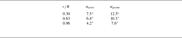
 αaero
αaero αgeom
αgeom V∞=7ms−1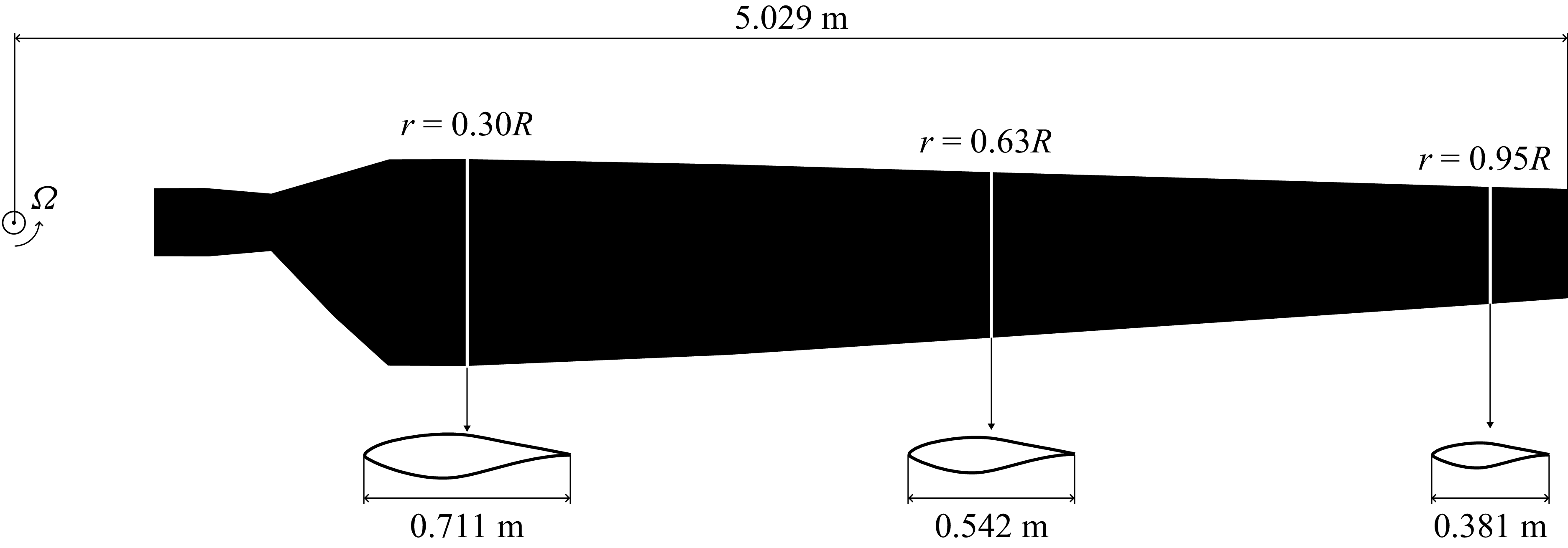
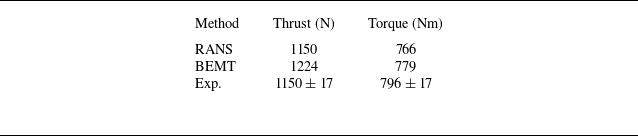
 ±
±

 r/R=0.8
 αaero
αaero αgeom
αgeom J
J

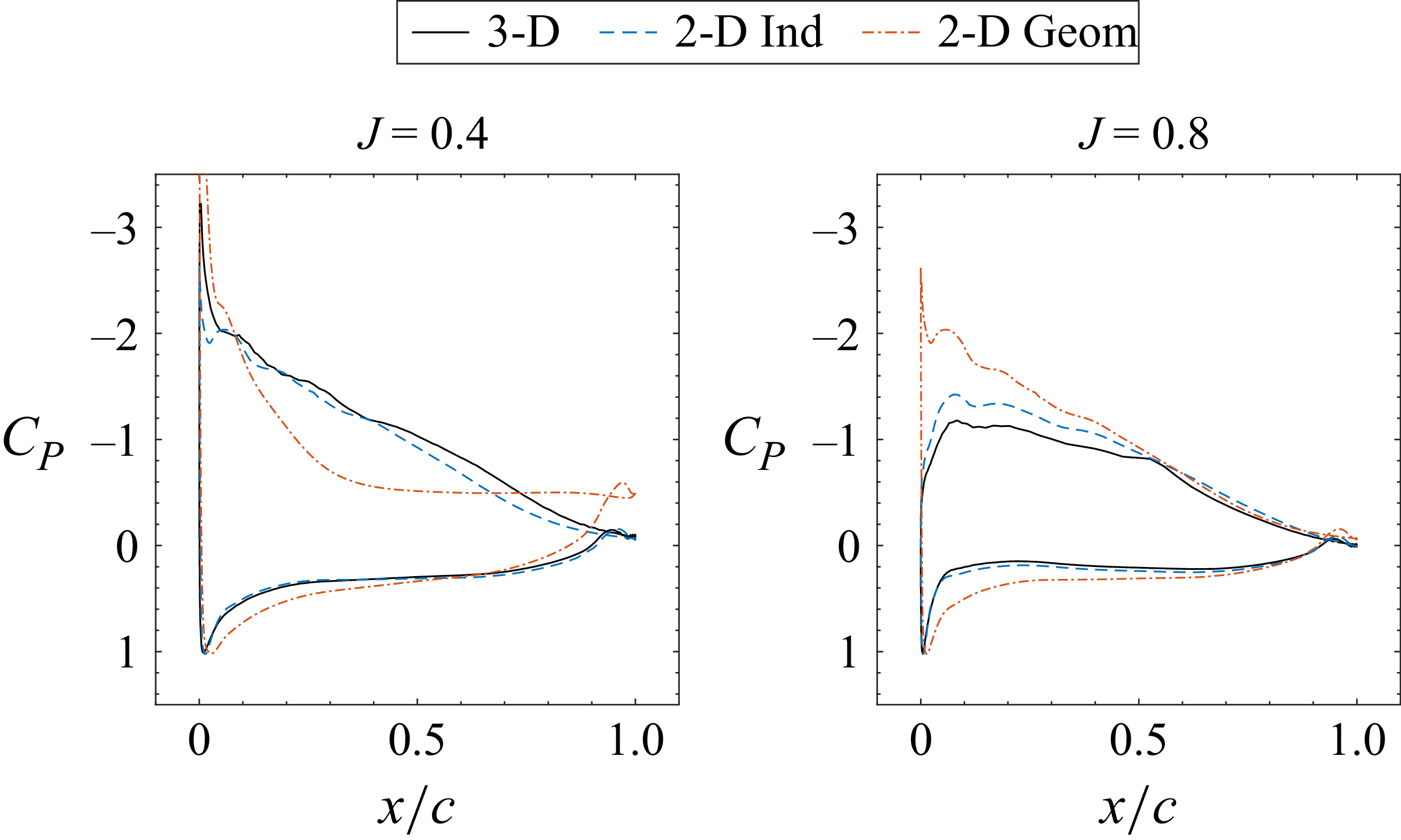

 β^
β^ s=0
s=0 s=±1
s=±1 s≤0
s≤0 ⋅⋅
⋅⋅ r/R=0.63
 J=0.8
J=0.8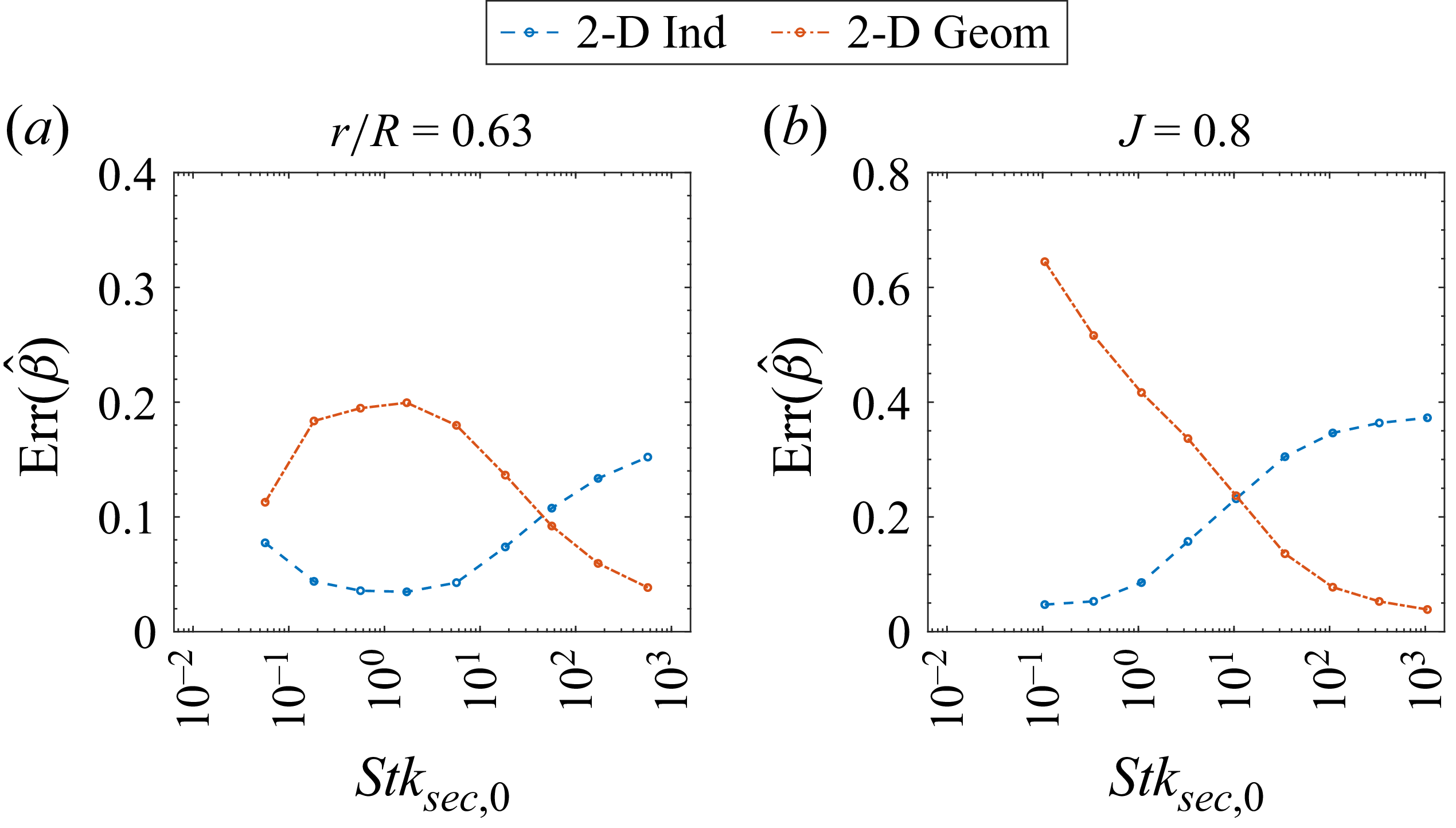
 r/R=0.63
 J=0.8
J=0.8
 t=0
t=0 Stkind
 ψ(Rep)=1
 rp(t=0)=0.95R
 rp(t=0)=0.80R
 V∞=5vf,ind(0,0)⋅x^
 V∞=50vf,ind(0,0)⋅x^
 1/(1+Stkind)
 r/R=0.20,0.40,0.60,0.80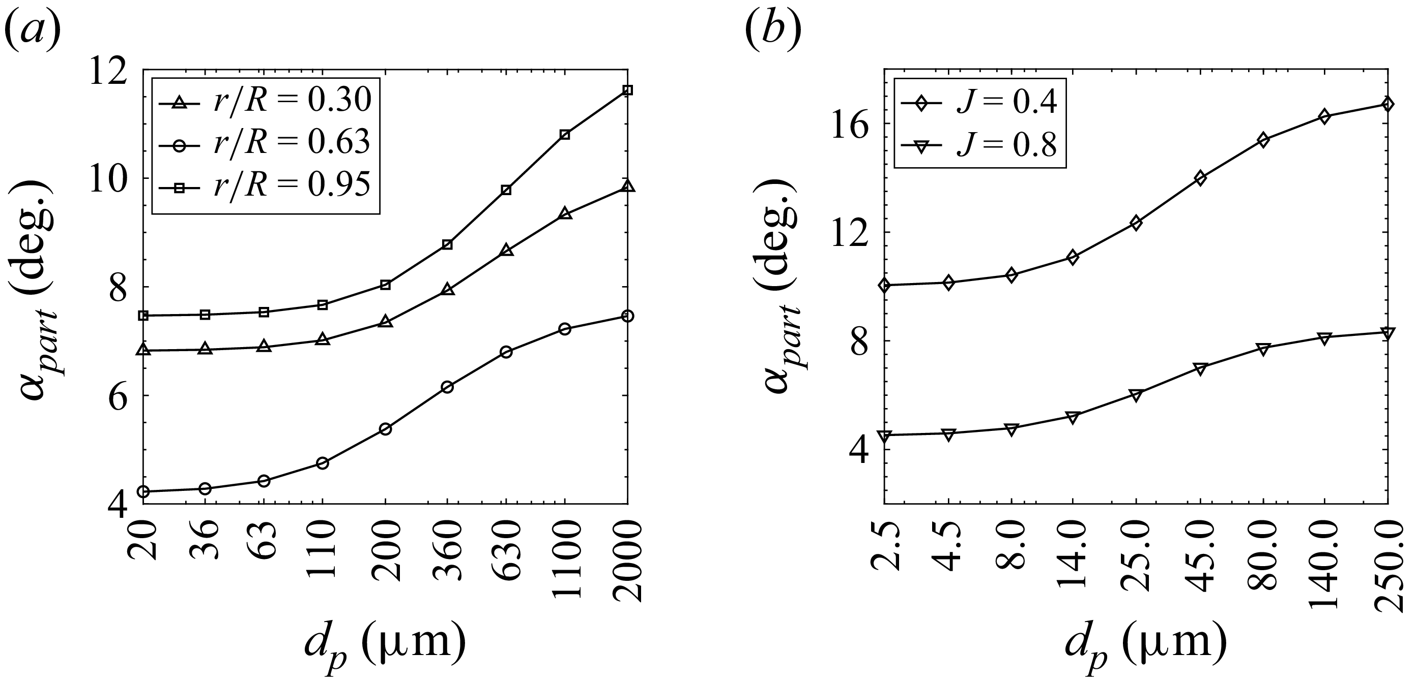

 r/R=0.30
 r/R=0.63
 r/R=0.95
 r/R=0.80
 J=0.4
J=0.4 J=0.8
J=0.8 dp=3600μm
 r/R=0.30
 Stkind>10
 β^
β^ s
s ∘
∘ αpart
αpart ⋅⋅
⋅⋅
 s
s r/R=0.8
 J=0.4
J=0.4 J=0.8
J=0.8
 r/R=0.95
 dp=200μm
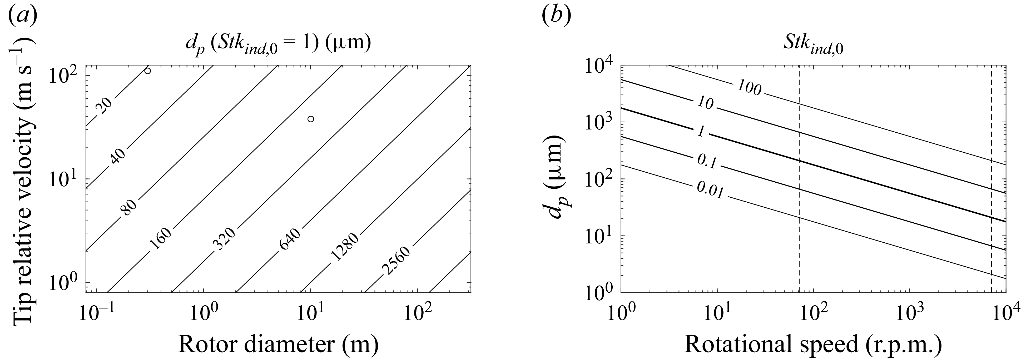
 dp
dp μm
μm Stkind,0=1
 ∘
∘ Stkind,0
 ΩR≫V∞
ΩR≫V∞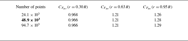
 CFinv(r)
 r
r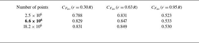
 7ms−1
7ms−1 CFinv(r)
 r
r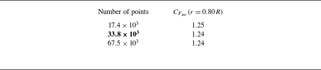
 CFinv(r)
 r
r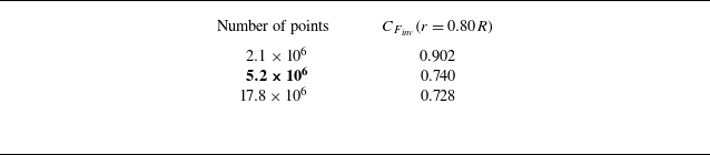
 J=0.8
J=0.8 CFinv(r)
 r
r

