


1. Introduction
Vorarlberg is the westernmost state of Austria and located in the Central Eastern and Northern Limestone Alps. The region is undergoing rapid glacier decline and most of the remaining glaciers and ice bodies are very small ( $ \lt 0.5$ km $^2$, Fischer and others, Reference Fischer, Seiser, Stocker Waldhuber, Mitterer and Abermann2015, Reference Fischer, Schwaizer, Seiser, Helfricht and Stocker-Waldhuber2021). Glacierized terrain is found in four subregions of Vorarlberg: Silvretta, Rätikon, Verwall and Lechtal. To quantitatively track ongoing glacier recession, frequent repeat mapping of glacier outlines is needed at sufficient spatial resolution to resolve very small features (Fischer and others, Reference Fischer, Schwaizer, Seiser, Helfricht and Stocker-Waldhuber2021).
This poses a number of challenges. As glaciers rapidly lose area and volume, features split or disintegrate and the relative amount of debris-covered ice tends to increase, which complicates the task of delineating glacier outlines in optical imagery (e.g., Paul and others, Reference Paul, Rastner, Azzoni, Diolaiuti, Fugazza and Le Bris2020; Linsbauer and others, Reference Linsbauer2021; Fischer and others, Reference Fischer, Schwaizer, Seiser, Helfricht and Stocker-Waldhuber2021; RGI 7.0 Consortium, 2023; Securo and others, Reference Securo, Del Gobbo, Baccolo, Barbante, Citterio and De Blasi2025). The accuracy with which very small features can be mapped further depends on the resolution of the underlying data. In glacier inventories compiled from 10–30 m resolution Sentinel-2 and Landsat imagery, size thresholds are commonly applied to exclude features that cannot reliably be identified. A minimum feature size of 0.01 km $^2$ is typically recommended (Paul and others, Reference Paul, Barry, Cogley, Frey, Haeberli and Ohmura2009). However, in regions with many very small glaciers and ice bodies, such an approach can lead to an undersampling of the existing ice extent (Fischer, Reference Fischer2018). This has important implications for our understanding of local hydrology (e.g., influence of remaining ice on water temperature (Boardman and others, Reference Boardman2025; Brighenti and others, Reference Brighenti2025)) and cryosphere-related natural hazards (Huss and Fischer, Reference Huss and Fischer2016; Fischer and others, Reference Fischer, Schwaizer, Seiser, Helfricht and Stocker-Waldhuber2021). In some regions, small ice features can also be of particular interest for glacier archaeology (e.g., Grosjean and others, Reference Grosjean, Suter, Trachsel and Wanner2007; Hafner, Reference Hafner2012; Ødegård and others, Reference Ødegård, Nesje, Isaksen, Andreassen, Eiken and Schwikowski2017; Pilø and others, Reference Pilø, Barrett, Eiken, Finstad, Grønning and Post-Melbye2021; Andreassen and others, Reference Andreassen, Nagy, Kjøllmoen and Leigh2022).
In addition to limitations defined by the characteristics and resolution of the data basis, more fundamental questions arise as glacier loss proceeds: at what point do glaciers cease to be glaciers? What do they become, and how should these features be treated and categorized in inventories? Cogley and others (Reference Cogley2011) define a glacier as ‘a perennial mass of ice, and possibly firn and snow, originating on the land surface by the recrystallization of snow or other forms of solid precipitation and showing evidence of past or present flow’. They suggest the term ‘ice body’ for ‘any object that is made mainly of ice and may or may not be a glacier’. Leigh and others (Reference Leigh, Stokes, Carr, Evans, Andreassen and Evans2019) proposed a scoring system that assigns a categorical ‘confidence level’ to features based on the presence or lack of crevasses, bergschrunds and visible ice. Linsbauer and others (Reference Linsbauer2021) applied criteria such as ‘no evidence of ice flow’ to determine features to be excluded from the most recent Swiss glacier inventory, thereby adhering to the requirement of ‘evidence of past or present flow’ given in Cogley and others (Reference Cogley2011).
Very high-resolution orthophotos generally allow detailed mapping of glacier features smaller than 0.01 km $^2$ (e.g., Fischer and others, Reference Fischer, Huss, Barboux and Hoelzle2014; Leigh and others, Reference Leigh, Stokes, Carr, Evans, Andreassen and Evans2019). Elevation change information derived from high-resolution digital elevation models (DEMs) can further support the identification of glacier boundaries particularly under debris cover, improving the mapping accuracy and enabling volume change computations for individual features (Abermann and others, Reference Abermann, Fischer, Lambrecht and Geist2010; Fischer and others, Reference Fischer, Huss, Barboux and Hoelzle2014, Reference Fischer, Schwaizer, Seiser, Helfricht and Stocker-Waldhuber2021; Fischer, Reference Fischer2018; Linsbauer and others, Reference Linsbauer2021; Hartl and others, Reference Hartl, Helfricht, Stocker-Waldhuber, Seiser and Fischer2022).
Glacier recession and the changing Alpine landscape in Vorarlberg are relevant to tourism and recreational activities (hiking, mountaineering) and some of Vorarlberg’s glacierized catchments are used for hydropower production. The regional government aims to track the evolution of the remaining glaciers to provide public information on environmental change. In this spirit, the work presented here provides an overview of the evolution of glaciers and ice bodies in Vorarlberg since the mid-2000s and considers change rates between 2017 and 2023 in more detail based on glacier outlines mapped using multi-temporal high-resolution orthophotos and DEMs. We assess the mapping challenges associated with vanishing glaciers, focusing on how results differ with data types and between multiple analysts mapping the same feature. In addition to change assessments, we categorize the ice features remaining in Vorarlberg by the presence or absence of crevasses (i.e., evidence of ice flow) to determine how many ‘glaciers’ as per Cogley and others (Reference Cogley2011) are left in the state. We note that this level of detail in visual analysis is only possible with very high-resolution imagery, as is available for the study region.
2. Study region and previous glacier inventories
Vorarlberg borders on Liechtenstein and Switzerland in the west and south, on Germany in the north and on the neighboring Austrian state of Tyrol in the east (Fig. 1a). With the exception of the region near Lake Constance in the northwest, much of the state is comprised of mountainous terrain. The highest peaks are found in southern part of the state in the Silvretta range (Piz Buin, 3312 m a.s.l.) along the border with Switzerland. Vorarlberg’s westernmost glaciers are found in the Rätikon range on the border to Switzerland on peaks just shy of 3000 m a.s.l. Both the Rätikon and the Silvretta are part of the Central Eastern Alps and drain into the river Ill and subsequently into the Rhine. The Verwall and Lechtal ranges span the eastern border of Vorarlberg and extend into Tyrol. The Verwall is considered part of the Central Eastern Alps and stretches to the border of the Northern Limestone Alps in the northwest. The Lechtal range is fully situated in the Northern Limestone Alps and drains towards the north via the river Lech.
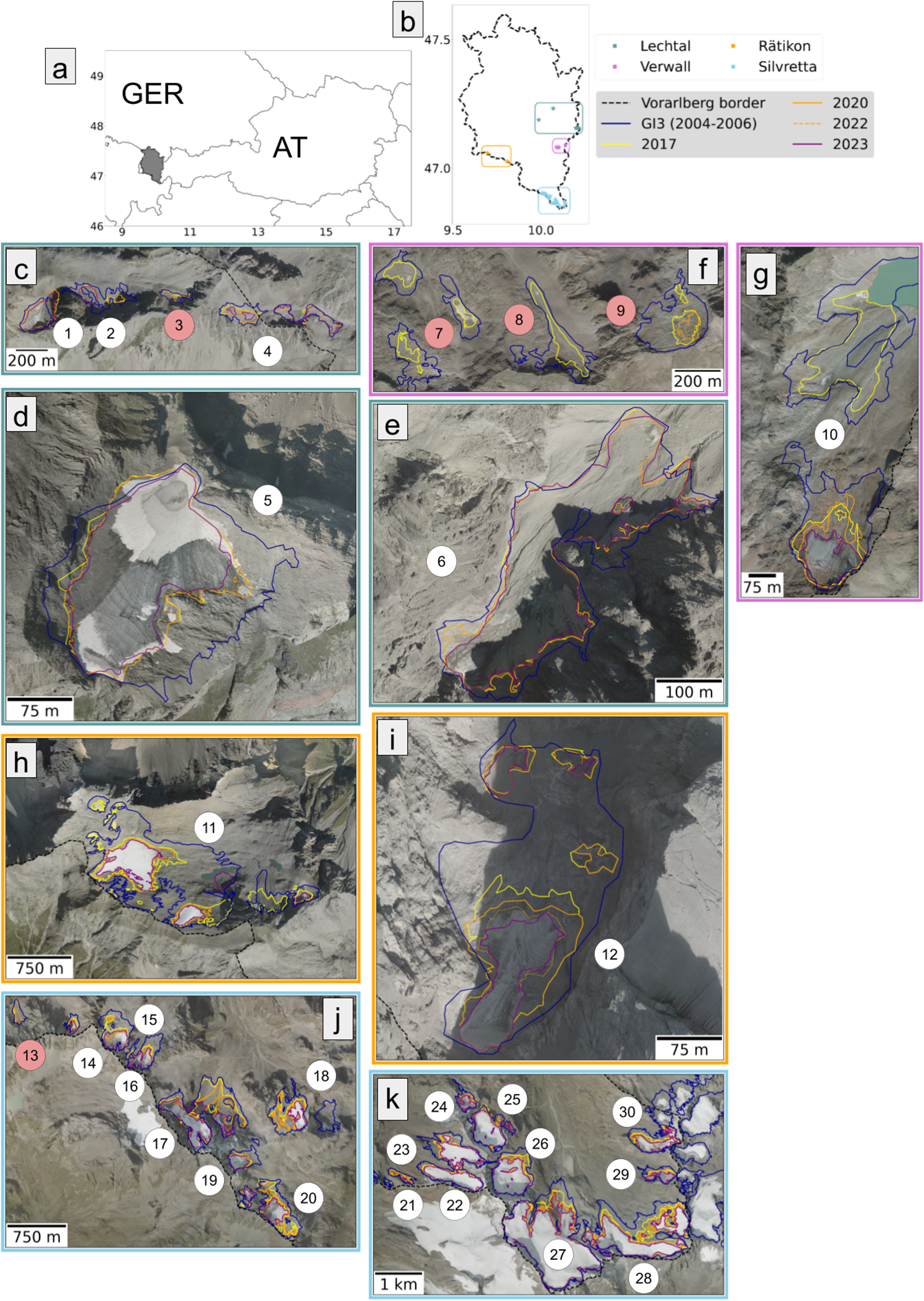
Location of Vorarlberg in Austria (grey, panel a), location of the four mountain regions in Vorarlberg (b, colored markers correspond to the centroids of the numbered glaciers shown in the panels). Glacier outlines shown over the 2022 orthophoto: Panels c, d and e: Lechtal; panels f and g: Verwall; panels h and i: Rätikon; and panels j and k: Silvretta. Glaciers are numbered sequentially for easier referencing in the following text. The individual panels without numbering are available in the supplementary material as image files to provide a more detailed visual. Red numbers indicate glaciers that vanished since 2017.

Mean annual air temperature in Austria in 1991–2020 was 1.98 $^{\circ}$C over the pre-industrial (1850–1900) baseline (Formayer and others, Reference Formayer2025; Huppmann and others, Reference Huppmann, Keiler, Riahi and Rieder2025). Warming has been especially pronounced since the 1980s, with temperatures increasing at a rate of 0.5 $^{\circ}$C per decade. In the 5 year period 2019–23, mean annual air temperatures were 2.7 $^{\circ}$C above pre-industrial (Formayer and others, Reference Formayer2025). High-resolution gridded climate data for Vorarlberg (Hiebl and Frei, Reference Hiebl and Frei2016, Reference Hiebl and Frei2018; https://atlas.vorarlberg.at/derklimapass; last access 13 Dec 2025) show a temperature increase of 1.2 $^{\circ}$C from 1961–90 to 1991–2020 at an example grid point in the Rätikon (Brandner Glacier, 2599 m a.s.l.). Overall precipitation in the study region does not show strong trends but snow cover is declining. At Brandner Glacier, the annual number of days with snow cover has decreased by 28 between the 1961–90 and 1991–2020 reference periods. The average environmental equilibrium line altitude in the study region was 2974 m a.s.l. in 1971–2000 (nearest grid point extracted from Žebre and others (Reference Zebre, Colucci, Giorgi, Glasser, Racoviteanu and Del Gobbo2021)), underscoring that the remaining glaciers in Vorarlberg cannot regain equilibrium with the current climate and are expected to disappear under future warming scenarios (Formayer and others, Reference Formayer2025).
The glacier area in Vorarlberg has been tracked in various national and regional inventories. Outlines from the Austrian national glacier inventories (GI1, GI2, GI3: Patzelt, Reference Patzelt1980; Kuhn and others, Reference Kuhn, Lambrecht and Abermann2013; Fischer and others, Reference Fischer, Seiser, Stocker-Waldhuber and Abermann2015) and additional, local and regional sources are compiled into a combined dataset and made available by the geodata service of state (https://vogis.vorarlberg.at, last access 2 Mar 2025). A fourth national inventory (GI4: Buckel and Otto (Reference Buckel and Otto2018)) was compiled using a different data basis and approach and shows minor inconsistencies with GI1-3. Approximately 80% of the state’s glacierized area is located in the Silvretta (Fig. 1j and k), followed by the Rätikon with 14% (Fig. 1h and i). Glacierized area in these regions declined from 13.26 km $^2$ to 10.29 km $^2$ between GI1 (1969) and GI3 (2004–06), equivalent to a regional change rate of $ \lt 1$% per year.
An additional regional inventory of glacier outlines for 2017 consistent with GI3 is available for the Silvretta (Fischer and others, Reference Fischer, Schwaizer, Seiser, Helfricht and Stocker-Waldhuber2021, Reference Fischer, Stocker-Waldhuber, Seiser, Helfricht and Schwaizer2021b). The updated glacier outlines produced for the study presented here build upon the most recent outlines available for the respective subregions, that is, GI3 for Lechtal, Rätikon and Verwall, and the 2017 inventory for the Silvretta.
3. Datasets
We aim for consistency with the three national glacier inventories cited above (GI1–3) and follow the methodology applied therein as much as possible. Like the outlines of GI3, the new outlines presented here are based on aerial imagery and DEMs derived from airborne laser scanning surveys (Table 1). All outlines produced for this study refer to the glacier names and unique ID-numbers as established in GI3.
Overview of digital elevation models and orthophotos used to map glacier outlines and compute volume change in the Vorarlberg mountain ranges, Silvretta, Verwall, Rätikon and Lechtal. The spatial resolution of the DEMs is 0.5 m. The resolution of the orthophotos is 0.1 m except for ‘orthophoto 2’, which has a resolution of 0.2 m. Orthophoto 2 was produced by the Austrian Federal Office of Metrology and Surveying (BEV); all other data were produced by the geodata office of the state of Vorarlberg.

Table 1 lists the datasets used for mapping the outlines presented in this study. Data were either provided directly by the regional government of Vorarlberg or accessed via their geodata portal (https://vogis.vorarlberg.at/, last access 28 Sept 2025). The vertical and horizontal accuracy ( $\sigma_v$, $\sigma_h$) of the DEMs was determined by the data provider based on comparison with ground control areas in stable terrain outside of glacierized regions. For both DEMs (2017 and 2023 acquisitions), $\sigma_v$ = $\pm$0.05 m and $\sigma_h$ = $\pm$0.1 m. We refer to Fischer and others (Reference Fischer, Schwaizer, Seiser, Helfricht and Stocker-Waldhuber2021) and the data report for the 2017 laser scanning survey (Würländer, Reference Würländer2019) for additional information on the DEM-related data processing. Mean elevation and slope angles were extracted for each glacier based on the DEMs resampled to 5 m resolution.
The orthophotos and laser scanning data were largely acquired between August and September (Table 1). In the 2020, 2022 and 2023 orthophotos, thin snow cover from small summer snowfalls is present on some of the glaciers in the Silvretta. For some glaciers, the 2023 orthophoto acquired at the same time as the DEM still shows seasonal snow cover. This is particularly pronounced in Lechtal. A second orthophoto was acquired later in the year and an additional mosaic was generated by the Austrian Federal Office of Metrology and Surveying (BEV). This is referred to as ‘orthophoto 2’ in Table 1 and also accessible via the Vorarlberg geodata portal; the Vorarlberg-specific orthophoto acquired concurrently with the DEM is referred to as ‘orthophoto 1’.
4. Methods
4.1. Mapping of feature extent
Unless stated otherwise, we use the term glacier to refer to the glaciers as listed in GI3. A glacier can be composed of multiple disconnected parts, which we refer to as fragments. For the subregions Verwall, Rätikon and Lechtal, the GI3 (2006, Fischer and others, Reference Fischer, Seiser, Stocker-Waldhuber and Abermann2015) outlines were used as a starting point for this study. For the Silvretta, the regional set of outlines for 2017 (Fischer and others, Reference Fischer, Schwaizer, Seiser, Helfricht and Stocker-Waldhuber2021) was used.
We use the numbering in Fig. 1 to more easily refer to specific glaciers in this text. The original inventory IDs are maintained in the data files. In cases of fragmentation, the fragments retain the ID of the original glacier, that is, multiple fragments can have the same ID and together comprise that particular glacier. In the dataset, these fragmented glaciers are multi-part polygons. This is in line with the approach taken in GI1, 2 and 3. For fragment-specific analyses, each fragment was assigned an additional ‘child’ ID while retaining the overall ‘parent’ glacier ID.
New outlines of glacier features were mapped manually, starting with the most recent prior outline. The 2020 and 2022 boundaries were mapped based on visual inspection of the respective orthophotos. In 2017 and 2023, the orthophotos as well as hillshades derived from the 2017 and 2023 DEMs and, for 2023, elevation change information were used to support the identification of the feature boundaries. In 2023, orthophoto 1 was generally used in combination with the 2023 DEM and derived information. Orthophoto 2 was used in rare cases where orthophoto 1 was not available or of poor quality. For debris-covered ice, it was assumed that the ice beneath the debris had melted if no or very little elevation change was apparent within the 2017 boundary. No common threshold for minimum elevation change was set, but most analysts chose to exclude areas where elevation change was substantially lower than over areas they visually confirmed to be ice.
All analysts had prior experience with mapping glacier outlines based on similar underlying data. The analysts were asked to map the outlines to the best of their abilities, given the data available for a given year. In general, the same analysts mapped the same regions and glaciers for all time steps, with some exceptions at individual glaciers in Lechtal and Verwall. Due to variations in snow cover and data availability (orthophotos only vs. orthophotos, DEMs and DEM-derived data), a few cases arose in which outlines were drawn beyond the previous glacier extent. For example, if ice was apparent in the 2023 image in an area not included in the 2022 outline, the 2023 outline would be extended to include this area. The prior outlines were not adjusted to ‘match’. This decision was guided mainly by analysts’ practical concerns about the feasibility of consistently backwards adjusting outlines every time new imagery becomes available.
All outlines were checked by at least two people and complex cases were discussed within a larger group. It was apparent that it is often challenging to definitively identify the ice boundary of very small, partially or fully debris-covered features, and that the interpretation of the imagery and DEM-derived data can differ substantially between analysts in such cases.
Previous inventory studies from the Austrian Alps estimated uncertainties in the glacier area of  $\pm$1.5% for glaciers larger than 1 km $^{2}$ and $\pm$5% for smaller glaciers based on mapping of example glaciers by ‘two parties’ (Abermann and others, Reference Abermann, Lambrecht, Fischer and Kuhn2009, Reference Abermann, Fischer, Lambrecht and Geist2010). To broadly assess uncertainties in our study region, we chose three test cases—Ochsentaler Glacier (Nr 27 in Fig. 1, inventory ID 12008), Schindler Glacier (Nr 4 in Fig. 1, ID 18006) and a nameless glacier (Nr 6 in Fig. 1, ID 19001)—that were mapped by multiple analysts based on 1) orthophotos and 2) DEMs and derived hillshades, starting with an outline for 2017 that was provided to the analysts for the purpose of the experiment. Ochsentaler Glacier is a relatively large glacier (approx. 1.9 km $^{2}$ in 2023) with limited debris cover and was selected as an example of a relatively ‘simple’ test case. The other two test cases are both located in Lechtal and were chosen as examples of features that are very challenging to map due to extensive debris cover and ‘inconclusive’ patterns of elevation change.
For each test glacier and data type (orthophotos or DEM-derived information), we computed the mean area and standard deviation over all outlines produced by the analysts and used the percentage ratio of the standard deviation to the mean as a measure of relative uncertainty. For glacier Nr 4 (Schindler Glacier), analysts were provided the orthophoto for 2022 and ‘orthophoto 2’ for 2023. Orthophoto 2 was acquired in September (Table 1), whereas the 2023 DEM was acquired in August. The analysts were not provided the orthophoto matching the acquisition date of the DEM, with the intention of highlighting the additional challenges of differing conditions even in the same summer season. ‘Orthophoto 1’, acquired on the same day as the 2023 DEM, shows noticeably more snow cover than orthophoto 2 from September 2023 (Fig. S2). The differences in snow cover are the assumed cause of positive elevation change at this glacier. For glacier Nr 6, analysts were provided the 2023 orthophoto matching the DEM acquisition date. Seasonal snow cover was also present at this site during the acquisition and the elevation change pattern is complex.
The above experiment informed the following uncertainty estimates for glacier features in the study region. However, we note that quantifying uncertainties is complicated by the glacier-specific challenges presented by very small, fully or partially debris-covered features. The following estimates aim to provide a general impression of how uncertainties in mapping change with fragment size and characteristics.
• Fragment area $ \gt $ 1 km
$^{2}$:
$\pm$1.5% (based on previous studies)
$ \gt $ 1 km
$^{2}$:
$\pm$1.5% (based on previous studies)• 1 km
$^{2} \gt $ Fragment area
$ \gt = 0.1$ km
$^{2}$:
$\pm$5% (based on previous studies)• 0.1 km
$^{2} \gt $ Fragment area
$ \gt = 0.05$ km
$^{2}$:
$\pm$10% (estimate aiming to allow for some fragments with higher uncertainties and some with lower uncertainties depending on the amount of debris cover)• Fragment area
$ \lt 0.05$ km
$^{2}$: 25% (estimate aiming to allow for some fragments with higher uncertainties and some with lower uncertainties depending on the amount of debris cover)


Area uncertainties for individual glaciers as per GI3 (i.e., all fragments associated with a given inventory ID) were computed from the values for individual fragments using standard error propagation. Uncertainties in area change were then computed from the glacier-wide uncertainty values.
4.2. Area change and feature categorization
Annual area change rates were computed for individual glaciers and regionally for the periods GI3 (2004–06) to 2017, 2017 to 2020 and 2020 to 2023. Due to high uncertainties, the 2022–23 period was omitted from the assessment of annual change rates.
For the 2023 glacier outlines, an additional assessment of individual fragments was carried out. Each polygon was categorized by size and checked visually for visible bare ice and crevasses. The fragments were given binary scores indicating the presence/absence of crevasses and visible bare ice, independent of the fragments’ association with a particular inventory ID. Statistical metrics were computed to assess which and how many fragments meet the criteria of ‘past or present flow’ (i.e., crevasses) as per Cogley and others (Reference Cogley2011).
4.3. Volume change
Volume changes between 2017 and 2023 were derived from difference rasters of the respective DEMs and the 2017 glacier outlines. Total volume change per glacier was computed as the mean elevation change within the respective 2017 outline multiplied with the 2017 glacier area. Volume change errors were calculated assuming independent errors in elevation change and area. Using the  $\sigma_v$ values of the DEMs ( $\pm$0.05 m), the mean error of 2017 to 2023 elevation change amounts to $\pm$0.07 m (root sum of the squares). We neglect a detailed analysis of spatial error correlations in elevation change due to the high quality and resolution of the laser-scanning-derived DEMs and the low magnitude of errors in elevation change compared to uncertainties in area and area change. Accounting for spatial error propagation based on heteroscadicity computations in tests with glaciers in the Silvretta following the approach of Hugonnet and others (Reference Hugonnet, Brun, Berthier, Dehecq, Mannerfelt and Eckert2022) with the Python package xDEM (xDEM contributors, 2024), we found glacier-wise errors of mean elevation change of about $\pm$ 0.05 m in all cases, confirming that the simplified approach is valid for our data set.
We computed average annual mass loss rates for individual glaciers for the 2017 to 2023 period by dividing the volume change by the number of years and the average area of the two time steps. Using the average area reduces the bias in geodetic mass balance introduced by using only the maximum area (Florentine and others, Reference Florentine, Sass, McNeil, Baker and O’Neel2023). However, the uncertainty in area change is higher than the uncertainty in area for a single time step and the uncertainty of the overall result increases accordingly. Volume was converted to mass assuming a standard bulk density of 850  $\pm$ 60 kg m $^{-3}$ (e.g., Huss, Reference Huss2013; Florentine and others, Reference Florentine, Sass, McNeil, Baker and O’Neel2023).
5. Results
5.1. Uncertainties in outline mapping of test cases
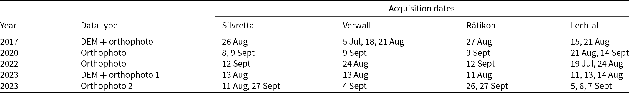
Five analysts mapped the outline of Ochsentaler Glacier (Nr 27) using the 2023 orthophoto, and subsequently with a hillshade and 2023–17 elevation change raster (Fig. 2). The relative uncertainty amounts to around 1% in both cases, in line with estimates by previous studies (Abermann and others, Reference Abermann, Fischer, Lambrecht and Geist2010). Two of the analysts commented on difficulties related to shadows and debris cover on the eastern glacier tongue and the largest discrepancies between outlines are found in this section. One analyst noted they found it very hard to tell where the ice under the debris cover ends in the orthophoto and commented that ‘the difference raster helps a little, but uncertainties are still high’. The outlines derived from the orthophoto (Fig. 2b) generally encompass a larger area than those derived from the hillshade and difference raster (Fig. 2c).
a: 2023 orthophoto of Ochsentaler Glacier (Nr 27 in Figure 1) with outlines mapped by five analysts. The outlines in red and orange tones were produced using only the orthophoto. The outlines in dark tones were produced using a hillshade derived from the 2023 DEM and the 2023–17 difference raster. The white box indicates the locations of the subset shown in panels b (orthophoto) and c (hillshade with difference raster overlay) EPSG:31254, grid in meters. All imagery obtained via https://vogis.vorarlberg.at/ (CC BY 4.0).

Averaging over the outlines produced for the comparison experiment, glacier Nr 4 (Fig. 3) covered about 0.007 km $^{2}$ and glacier Nr 6 (Fig. S1) had an area of about 0.05 km $^{2}$ in 2023. Relative uncertainties amount to 32–58% for glacier 4 and 22–36% for glacier 6 and depending on the year of the orthophoto and the data type.
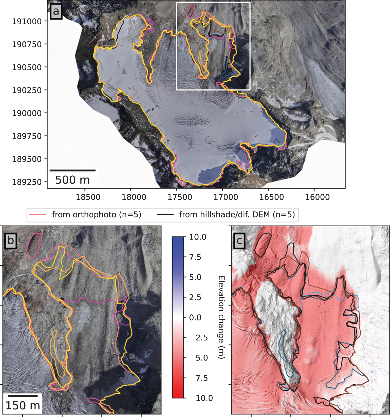
a: 2022 orthophoto, b: 2023 orthophoto, c: 2023 hillshade and d: 2023–17 elevation change for glacier 4 (Schindler Glacier) in the Lechtal region as provided to analysts for the mapping experiment. Colored lines show the outlines produced by the analysts using the respective orthophotos or the hillshade and difference raster. Additional orthophotos in Figure S2 illustrate differing snow cover during 2017 and 2023 DEM acquisitions, which is assumed to have caused the positive elevation change seen in panel d. EPSG:31254. All imagery obtained via https://vogis.vorarlberg.at/ (CC BY 4.0).

Regarding glacier 4, analyst 4 commented that presumably there is more ice than is visible in the orthophotos (Fig. 3a and b) and only the visible parts can be confidently identified. The same analyst commented that they chose a relatively wide outline in the upper section of the glacier when mapping with the 2023 hillshade (Fig. 3c) and difference raster (Fig. 3d) because they found it impossible to clearly identify the ice boundary and aimed to include any area that they thought might potentially contain ice. The positive elevation change at glacier 4 was not discussed with the analysts prior to the experiment and likely contributed to uncertainties in interpretation.
At glacier 6 (Fig. S1), the analysts considered the differing snow cover between the 2022 and 2023 orthophotos (Fig. S1a and b) a main source of uncertainty in addition to debris cover in the lower section of the glacier. One analyst noted that they did not find the elevation change information and hillshade (Fig. S1c and d) helpful for this test case and did not feel that the additional information reduced the uncertainties. Two analysts remarked on mosaicing errors in the 2023 orthophoto (Fig. S1b) and indicated that this created an additional challenge besides the issues related to snow and debris.
Figures S2 and S3 show the full time series of orthophotos for glaciers 4 and 6 as additional context, although analysts were asked to only consider the two orthophotos they were provided for the respective experiments. Examples of the mosaicing problem mentioned by the analysts are highlighted in panel d of Fig. S3.
5.2. Mapping challenges and discrepancies
Delineating ice boundaries under debris cover was identified as a key challenge for analysts and several glaciers show slight increases in area over time due to debris cover-related mapping discrepancies (refer to Table S1 in the supplement for areas of all glaciers in all years). For example, at Platten Glacier (Nr 14 in Fig. 1), a debris-covered section on the western side was included in the 2023 outline but was not mapped in prior outlines (Fig. S4). The analyst indicated that the outlines reflect their interpretation of the respective orthophotos and, for 2023, additional DEM-derived information. Similar discrepancies are present at Schweizer Glacier (Nr 15 in Fig. 1 and Fig. S5), which also shows a slight area increase between 2022 and 2023. Here, the analyst indicated that the elevation change raster suggests the presence of debris-covered ice, which was not mapped in previous years, presumably because it was not identifiable in the available orthophotos. At Brandner Glacier (Rätikon, Nr 11, Fig. S6), a previously unmapped fragment was included in the 2023 inventory based on inspection of the orthophoto and hillshade.
Glaciers 4 and 6 (discussed above in the mapping experiment) and Kaltenberg Ferner (Nr 10, Fig. S7) also show minor discrepancies between the 2020, 2022 and 2023 outlines. This is related to visual differences in the respective orthophotos (more snow in 2023, shadows, debris cover) and, for Kaltenbergferner, to an analyst change between 2022 and 2023. Discussion with the two analysts revealed differing interpretations of debris-covered parts, but the resulting discrepancies are considered to be within the expected uncertainty. The 2017 outline for this glacier includes a lower fragment, in keeping with GI3. The analyst decided that the 2017 orthophoto warranted including this fragment but found no more evidence of ice in the following years.
Analysts found mapping the remaining glacier features of the Lechtal particularly challenging. In addition to general issues related to debris cover, glaciers 4 and 6 show slightly positive mean elevation change of 0.12 and 0.03 m a $^{-1}$ for 2017 to 2023. This is assumed to be mainly caused by seasonal snow cover present during the 2023 DEM acquisition, but may also be related to debris input or mass gain from avalanches.
5.3. Area and volume change
The total ice-covered area in Vorarlberg decreased from 10.609 km $^{2}$ in GI3 (2004–06, Fischer and others, Reference Fischer, Seiser, Stocker-Waldhuber and Abermann2015) to 7.52 $\pm$ 0.07 km $^{2}$ in 2017 and to 5.27 $\pm$ 0.06 km $^{2}$ in 2023. For 2017 to 2023, this is equivalent to a loss of 30% of the 2017 area, or an average loss rate of 5% a $^{-1}$. Percentage area losses for the same period differ strongly between regions and were highest in the Verwall with $-$86% (relative to the 2017 area) and lowest in Lechtal with $-$24% (Table 2). Compared to the area change in the period GI3 to 2017, average loss rates since 2017 increased in all regions. In the more recent sub-periods 2017–20 and 2020–23, average annual loss rates increased with time in Lechtal and Silvretta and decreased in Rätikon and Verwall (Table 2).
Overview of glacier change since GI3. Percentage change is calculated in relation to the older outlines for each time step. The mean elevation change is given as the mean over the values at individual glaciers in a given region.
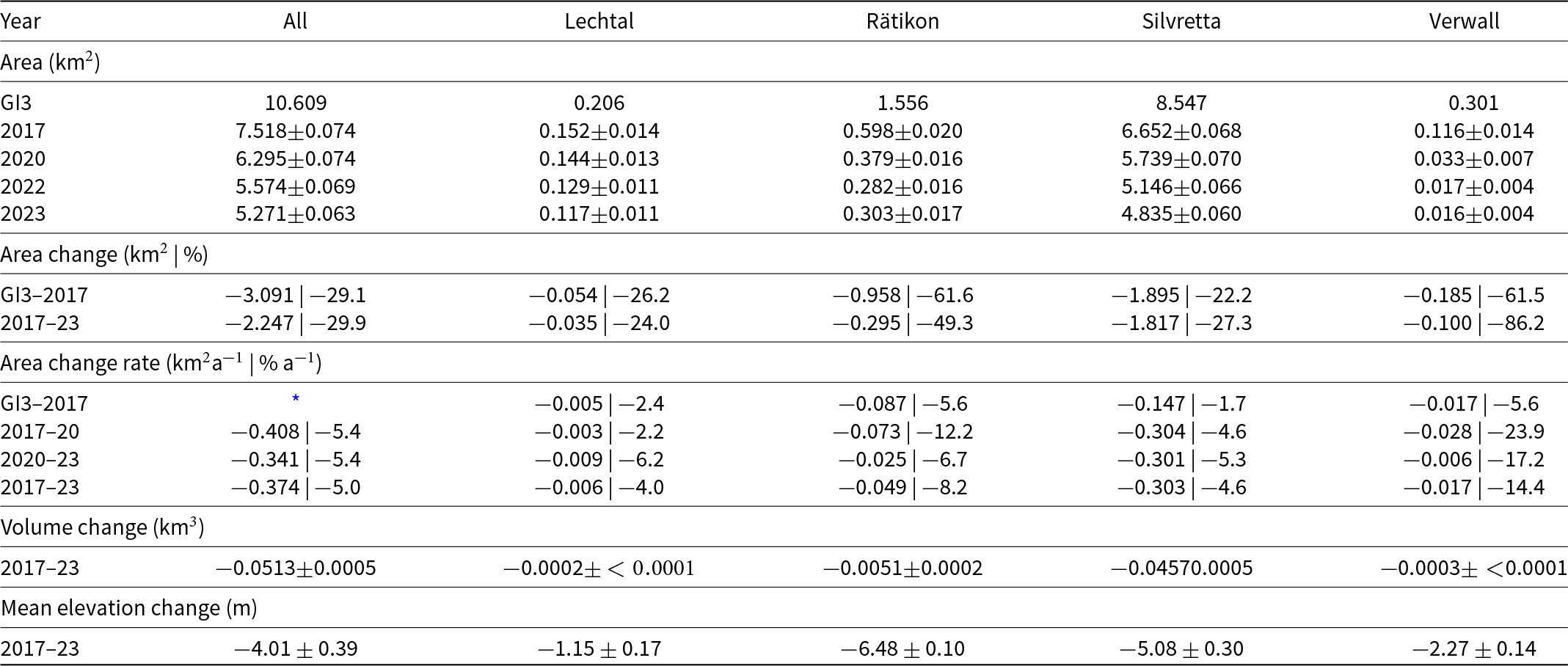
* GI3 (Fischer and others, Reference Fischer, Seiser, Stocker-Waldhuber and Abermann2015) refers to outlines for 2004 in the Silvretta and for 2006 in the other three regions. Annual change rates are only given per region to account for the different starting years. The GI3 dataset does not include area uncertainties; hence, they are omitted in the table.
Since 2017, five of the glaciers included in GI3 have vanished completely. In the Verwall, the westernmost glaciers (Mittlerer, Westlicher and Östlicher Eisentaler Gletscher, Nrs 7, 8 and 9 in Fig. 1) have vanished. Analysts found no evidence of remaining ice in the imagery. Similarly, the smallest of the six Lechtal glaciers (nameless, Nr 3) and the westernmost glacier in the Silvretta (Garnera Gletscher, Nr 13) showed no more evidence of ice in the 2023 data. In addition to the five glaciers that vanished completely, eight glaciers lost more than half of their 2017 area. In absolute terms, area losses between 2017 and 2023 were largest at the largest glaciers; Vermunt Glacier (Nr 28) lost 0.443 km $^{2}$ (35% of 2017 area), followed by Ochsentaler Glacier (Nr 27) with $-$0.285 km $^{2}$ ( $-$13%) and Brandner Glacier (Nr 11) with $-$0.284 km $^{2}$ ( $-$49%). Refer to Tables S1, S2 and S3 in the supplement for glacier areas, area change and change rates of all glaciers in the study region.
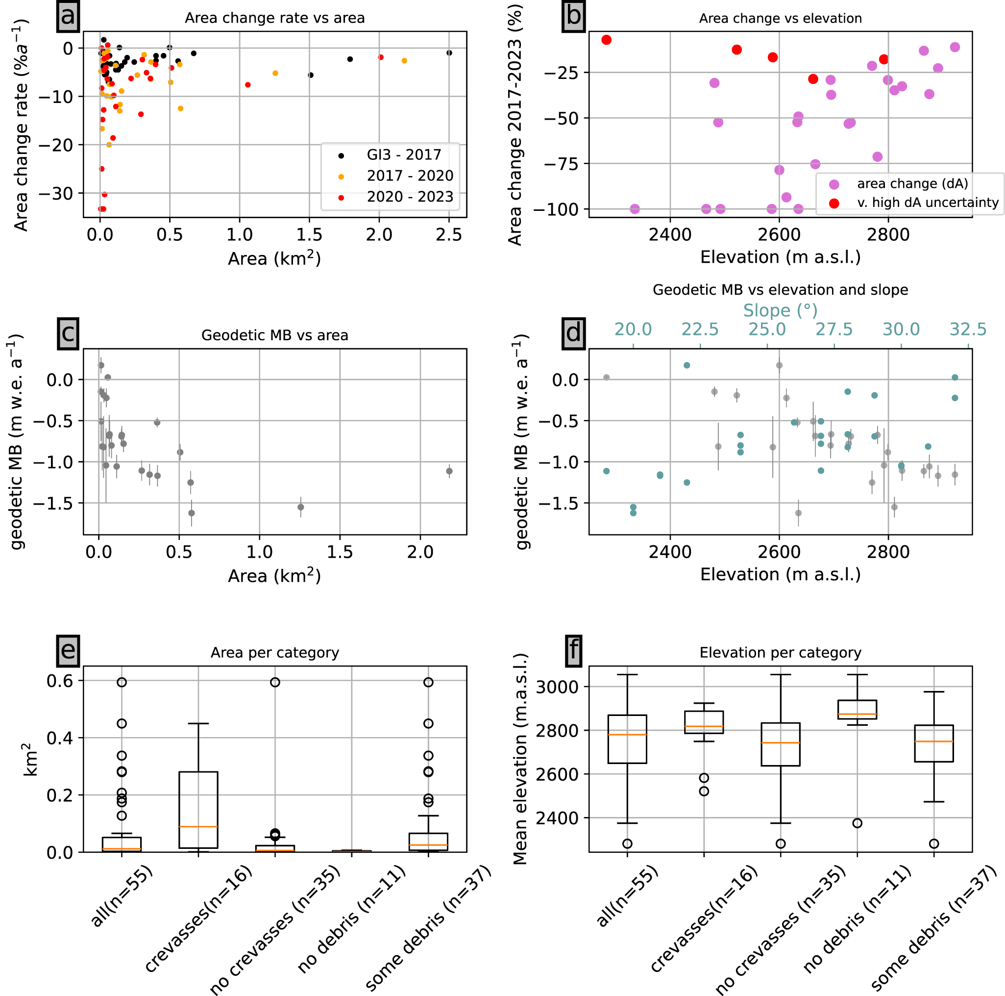
Figure 4a shows percentage area loss rates at individual glaciers for three sub-periods since GI3, confirming the trend towards increased loss rates for the recent periods compared to GI3–2017 (relative change rates in tabular form are provided in Table S3). The highest loss rates correspond to the glaciers that vanished completely between 2020 and 2023. The highest percentage area change values over the 2017–23 period (up to 100% at the vanished glaciers) are found at relatively low-elevation glaciers, but not all low-lying glaciers have correspondingly high area losses (Fig. 4b).
Panel a: Area change rate (% per year) vs. glacier area for the periods GI3–2017, 2017–20 and 2020–23. The  $x$-axis refers to the area of the older outline for each time step. Panel b: Percentage area change for 2017–23 vs. mean elevation of each glacier in 2017. Red markers indicate unreliable area change values where the uncertainty is greater than the change. Panel c: Geodetic mass balance against the 2017 glacier area. Panel d: Geodetic mass balance against 2017 mean glacier elevation (lower axis) and slope (upper axis). Panel e: Boxplots of 2023 feature size for: all mapped features, features with and without crevasses, features without debris and with some amount of debris. ‘n’ indicates the number of features per category. Features where data quality inhibited categorization were not counted and the single outlier points for the largest fragment (1.89 km $^2$) were omitted to better visualize the spread. Panel f: Boxplots of mean fragment elevation for the same categories as in e. The data in panels e and f are presented in tabular format in Table S5. Fragments with undetermined categories due to poor image quality are not counted.

The total volume change between 2017 and 2023 in the Silvretta was  $-$0.0513 $\pm$ 0.0005 km $^{3}$. The majority of these losses (89%) occurred in the Silvretta with $-$0.0457 $\pm$ 0.0005 km $^{3}$. Average elevation change amounted to $-$4.01 $\pm$ 0.39 m for the study region (equivalent to 0.67 m a $^{-1}$), with substantial variations between the subregions (Table 2). Geodetic mass balance at individual glaciers ranged from about $-$0.2 m w.e. a $^{-1}$ to about $-$1.5 m w.e. a $^{-1}$ (Table S4). The most negative values are found at relatively large glaciers (Fig. 4b). Geodetic mass balance tends to become more negative at glaciers with higher mean elevation and lower mean slope angles (Fig. 4d).
5.4. Fragmentation and feature classification
The amount of unfragmented glaciers (i.e., only one glacial fragment associated with one inventory ID) in the study region decreased from 73% in GI3 to 63% in 2017 and 54% and 52% in 2020 and 2023, respectively. A particularly pronounced change in fragmentation occurred at Brandner Glacier (Fig. S7), which consisted of three fragments in GI3 and had disintegrated into 20 fragments by 2017 (Table S1). Many of the smaller fragments vanished in the following years and only four fragments remained in 2023. Vermunt Glacier (Nr 28, Silvretta, Fig. S8) is a contrasting example where fragmentation increased over the study period from two fragments in GI3 and 2017 to nine fragments in 2023, respectively.
In 2023, 55 individual fragments were mapped, 29 of which were larger than 0.01 km $^2$. Crevasses were apparent at 16 fragments associated with 13 distinct IDs. 12 fragments were both larger than 0.01 km $^2$ and showed crevasses. Fragments smaller than 0.01 km $^2$ covered an area of 0.090 km $^2$, less than 2% of the total glacier area in the study region. Some amount of debris cover was apparent at 37 fragments (67% of all fragments). With a median area of 0.006 km $^2$, the fragments without crevasses were substantially smaller on average than those with crevasses (Fig. 4e and Table S5). Fragments with crevasses have a slightly higher mean elevation than those without and cover a narrower altitudinal range (Fig. 4f). Fragments without any debris cover are, on average, the smallest and highest of the assessed categories (Fig. 4e and f).
Summarizing the results of the classification efforts in the context of Cogley and others (Reference Cogley2011)’s definition of a ‘glacier’, 16 fragments (associated with 13 ID) have crevasses and hence may still be considered ‘glaciers’. The remaining 39 fragments (linked to 12 ID) meet the criteria for ‘ice bodies’ but not for ‘glaciers’ due to the lack of visible crevasses, that is, ‘evidence of past or present flow’ (Cogley and others, Reference Cogley2011). This implies that 13 ‘glaciers’ would be counted when applying the criterion of visible crevasses and remaining consistent with the counting approach of the previous inventories. Counting with the same criterion for crevasses but without reference to the existing inventory system yields 16 ‘glaciers’, whereas counting not using the criterion of visible crevasses yields 25 remaining glaciers.
6. Discussion
6.1. Recent glacier change in Vorarlberg: key takeaways
Glaciers in Vorarlberg are shrinking rapidly and several glaciers have already disappeared. Area loss rates have accelerated since the mid-2000s (GI3) across all four subregions. However, area loss rates show considerable variations between the four regions, individual glaciers and for the different subperiods (Table 2). Elevation change from 2017 to 2023 also varied substantially across regions, with lower values in Lechtal and Verwall than in Rätikon and Silvretta. Geodetic mass balance at smaller glaciers tends to be less negative than at the largest glaciers of the study region and appears to become more negative with increasing altitude (Fig. 4d and Table S4). That is, the data indicate that smaller, lower elevation glaciers are losing less mass per area than the larger, higher elevation glaciers. Uncertainties in area and area change are higher at smaller glaciers, contributing to greater overall uncertainties in geodetic mass balance.
We assume there are two main contributing factors:
1) Sections of thin ice that melted completely during the study period (2017–2023) produce a reduced elevation change signal compared to areas where ice remained thicker and melted throughout the entire time period. Considering the Verwall as an extreme example, three of the four glaciers counted in the 2017 Verwall inventory had vanished by 2023. This amounted to a very high relative area loss ( $-$86% in total, or $-$14% a $^{-1}$) and limited elevation change rate (0.34 m a $^{-1}$) for the 2017 to 2023 period. Similarly, the complete melting of thin fragments contributed to a reduced overall fragmentation of some glaciers (e.g., Brandner Glacier, Fig. S6). In contrast, some of the larger glaciers are still undergoing increasing fragmentation as areas of thin ice melt, connections to tributaries are lost, and newly emerging rock outcrops split previously connected features into multiple fragments (e.g., Vermunt Glacier, Fig. S8).
2) Small, sheltered glaciers may benefit from topographic effects like shading, wind drift or avalanche input (e.g., Florentine and others, Reference Florentine, Harper, Fagre, Moore and Peitzsch2018; Boardman and others, Reference Boardman2025), which can contribute to reduced mass losses compared to larger glaciers. It is difficult to separate such effects from biases introduced by remaining seasonal snow cover at some glaciers during the 2023 DEM acquisition and additional investigations would be needed to quantify such effects in a regional context. The trend towards less negative geodetic mass balance at lower elevations (Fig. 4d) could be interpreted as an indication that ice bodies that still remain at such comparatively low elevations can survive there because they are in topographically favorable locations and benefit from shading or terrain-related snow input. In addition, the glaciers with relatively low mass loss tend to be steeper on average (Fig. 4d) and may have shorter response times (e.g., Zekollari and others, Reference Zekollari, Huss and Farinotti2020).
Considering the categorization of individual fragments, those with crevasses are the largest category on average, in keeping with the expectation that ‘glaciers’ would generally be larger than ‘ice bodies’ that remain after ‘glaciers’ have strongly receded. Visual inspection of fragments in the smallest and highest ‘no debris’ category suggests that these are often located in steeper terrain above the margins of larger fragments that have receded, in areas with few loose rocks that would contribute to debris cover.
We note that the criterion of visible crevasses is not a perfect indicator of ‘past or present ice flow’. Crevasses may have been present in the past but are no longer visible in recent images due to snow, debris cover or ice melt. We consider this approach to defining ‘glaciers’ vs. ‘ice bodies’ the most practicable option for the study region but acknowledge that different terminology, definitions and classification schemes may be better suited in other regions with different glacier characteristics or data availability.
6.2. Reflecting on the methods: recommendations and limitations
The national glacier inventories for Austria (Patzelt, Reference Patzelt1980; Lambrecht and Kuhn, Reference Lambrecht and Kuhn2007; Kuhn and others, Reference Kuhn, Lambrecht and Abermann2013; Fischer and others, Reference Fischer, Seiser, Stocker Waldhuber, Mitterer and Abermann2015) and most inventories for subregions of Austria (e.g., Abermann and others, Reference Abermann, Lambrecht, Fischer and Kuhn2009; Fischer and others, Reference Fischer, Schwaizer, Seiser, Helfricht and Stocker-Waldhuber2021; Hartl and others, Reference Hartl, Schmitt, Schuster, Helfricht, Abermann and Maussion2025) have not applied size thresholds in the past. Accordingly, introducing size thresholds in new inventories would lead to inconsistencies and inhibit change assessments through time by removing small fragments that were previously counted towards a given glacier’s area. If high-resolution data is available for glacier mapping, it is of interest to retain as much detail as possible. The resulting feature outlines may then be filtered for specific applications—for example, comparisons with global inventories—by applying size thresholds or other criteria. This avoids potential undersampling of very small features (e.g., Fischer, Reference Fischer2018) and allows customized, application-dependent usage.
In terms of image quality, documenting rapid glacier change necessitates frequent mapping and it may not always be possible to select for ‘ideal’, snow-free imagery. Hence, systematic approaches to documenting data quality, surface conditions in particular images and other sources of uncertainty are needed. Including commentary and/or pre-defined flags in inventories that allow users to assess individual outlines in relation to the underlying data is essential for further interpretation. Such documentation also supports the workflow of updating and potentially correcting errors in existing outlines as new imagery or topographic data become available.
As glacier loss progresses and more and more glaciers turn into ‘ice bodies’, consistent usage of terminology becomes increasingly important for the systematic compilation of inventories as well as for public communication and outreach. We suggest using criteria such as visible crevasses as evidence of flow, or scoring systems (Leigh and others, Reference Leigh, Stokes, Carr, Evans, Andreassen and Evans2019) adapted to regional conditions and the type and resolution of available data. We note that mapping based on 10-30 m satellite imagery may require different criteria than sub-meter resolution imagery and/or the introduction of size thresholds to ensure that relevant surface features can be identified. For consistent change assessments over time, we recommend including ‘ice bodies’ in calculations of change in total glacierized area and providing supporting contextual information on the status of the features.
Even with high-resolution data, inherent uncertainties in the mapping process remain, as evidenced by the example cases in Figs. 2, 3 and the figures in the supplement. Central challenges are debris cover and other factors (snow, shadows) preventing the visual identification of the ice boundaries. Topographic data and elevation change information support mapping efforts in such cases but the added value is limited for complicated features with elevation change patterns that do not necessarily reflect ice loss exclusively (e.g., Figs. 3, S1 and S2).
Usage of different data types can also lead to undesired variations in the outlines. Analysts noted that changes in surface roughness visible in hillshades sometimes give an indication of where the ice ends that is not apparent in orthophotos and reported using hillshades in this way when available. This is evident in the outlines mapped from the hillshade and difference raster compared to the orthophoto at the example of Ochsentaler Glacier (Fig. 2b and c).
Reflecting on the comparison of outlines produced by different analysts, it was notable that some analysts took an approach that can be summarized as ‘map only what you can definitively see in a given image’, whereas others had a less clearly defined approach along the lines of ‘map areas that could still contain ice based on process understanding’, which also took into account prior knowledge of the feature’s outline and topography. For multiple analysts, consistency in mapping might be improved by agreeing upon common approaches to this and other issues. Debris cover appears to be the main source of discrepancies between outlines produced by different analysts, even if elevation change data are available. To reduce discrepancies, thresholds for inclusion or exclusion of areas with a set amount of elevation change might be defined. However, all analysts expressed that there is a limit to mapping glacier features in an advanced state of disintegration that is not primarily related to the type or spatial resolution of the data and rather inherent to the nature of the features.
Estimated relative uncertainties of over 50% of the total glacier area, as found for the example of glacier Nr 4 (Fig. 3) provide a quantitative indication that the utility of detailed manual mapping of such very small, often highly debris-covered and fragmented features is limited. Depending on the application, it may be useful to instead assign a point coordinate (e.g., the centroid of a former outline) or a specified value in a feature attribute to indicate the likely presence of remaining ice as well as large uncertainties and/or ‘nearly vanished’ status. We note that the elevation change—assumed to be due to a change in ice volume—can be computed with a high degree of accuracy within a given outline if high-resolution DEMs are available. Hence, ice loss for challenging features could still be tracked, provided there is no substantial elevation gain from debris input or snow cover.
We acknowledge that studies such as this one rely on high-resolution DEMs and orthoimagery, which usually have limited spatial coverage. Our work focuses on small glaciers in their final stages of existence and tracking their evolution requires a level of detail that may not be relevant or needed in regions of the world where most glaciers are multiple orders of magnitude larger.
7. Conclusion
The process of mapping the very small, fragmented glacier features in the mountains of Vorarlberg highlighted challenges associated with documenting the vanishing of glaciers. With very high-resolution imagery and topographic data, the main limitations are not related to the resolution of the data but rather inherent to the process of glacier disappearance. Being able to see tiny ice features in 10 cm resolution orthophotos does not necessarily mean that it is easy to delineate the boundary of the ice body, or clearly define the point at which an ice feature ceases to be a glacier.
In our study, debris cover was a main cause of mapping challenges and discrepancies between analysts. This reflects findings of Linsbauer and others (Reference Linsbauer2021) who describe similar challenges in their work documenting the most recent Swiss glacier inventory. They also report increasing relative area uncertainties with decreasing glacier size. Unlike the Swiss inventory (Linsbauer and others, Reference Linsbauer2021) and larger scale, Alps-wide or global inventories derived from Sentinel-2 and Landsat satellite imagery (e.g., Paul and others, Reference Paul, Barry, Cogley, Frey, Haeberli and Ohmura2009; Reference Paul, Rastner, Azzoni, Diolaiuti, Fugazza and Le Bris2020) we did not apply the common minimum size threshold of 0.01 km $^2$ with the aim of comprehensively documenting even the very small remaining glacier features of our study region and to remain consistent with previous work.
Even if glacier fragments in regions undergoing rapid ice loss could be mapped perfectly without any uncertainties, the question of how they should be categorized and counted would remain. In our study region, the number of remaining ‘glaciers’ varies by more than 40% depending on whether one counts any remaining ice within the area of a formerly inventoried glacier (25 remaining) or counts only fragments that show evidence of past or present ice flow (16 fragments of 13 previously inventoried glaciers). Additional considerations, such as introducing a minimum size threshold, produce additional variability in the result of ‘counting glaciers’. Arguably, such issues are of limited scientific relevance. However, clear terminology and accessible explanations of ongoing processes are important when discussing the vanishing of glaciers in public communication and outreach activities. We hope this study and the example of the vanishing glaciers of Vorarlberg can contribute to the ongoing discourse on these topics within the scientific community.
Supplementary material
The supplementary material is available at https://doi.org/10.1017/aog.2026.10044
Data availability
The glacier outlines produced for this study are available from Conzelmann and others (Reference Conzelmann2026): https://doi.pangaea.de/10.1594/PANGAEA.984116.
Acknowledgements
The scientific editor and two anonymous reviewers provided thorough and constructive feedback that improved the manuscript. Thank you very much! The regional government of Vorarlberg provided partial financial support for this work. The authors thank Jakob Heinzle and Andreas Marlin at the geodata office of the state of Vorarlberg for providing data support and background information related to data acquisition and processing. We gratefully acknowledge the Open-Access Fund of the Austrian Academy of Sciences, which covered the publication costs for this paper.


 Open access