


1. Introduction
Turbulent mixing in the stratified ocean interior, originating from internal gravity wave breaking (MacKinnon et al. Reference MacKinnon2017), plays a central role in determining the global distributions of carbon, heat, nutrients, plankton and other salient tracers (Wunsch & Ferrari Reference Wunsch and Ferrari2004). Kelvin–Helmholtz (KH) instability is arguably one of the key mechanisms generating such small-scale turbulence and diapycnal mixing (Caulfield Reference Caulfield2021; Dauxois et al. Reference Dauxois2021). Wind-induced shear in the surface mixed layer can render the internal (or interfacial) gravity waves at the pycnocline unstable, causing the interface to roll up into billow-like structures – the hallmark of KH instability (Smyth & Moum Reference Smyth and Moum2012). This paper digresses from the typical studies on KH instability where the background shear flow is assumed to be steady, for example, see Caulfield & Peltier (Reference Caulfield and Peltier2000), Mashayek & Peltier (Reference Mashayek and Peltier2012), Rahmani, Lawrence & Seymour (Reference Rahmani, Lawrence and Seymour2014) and Mashayek, Caulfield & Alford (Reference Mashayek, Caulfield and Alford2021). Instead, our study is motivated by settings where the background shear has an explicit time dependence, periodic to be specific. During the summer seasons, shelf seas (Mihanović et al. Reference Mihanović, Orlić and Pasarić2009; Guihou et al. Reference Guihou, Polton, Harle, Wakelin, O’Dea and Holt2018), lakes (Lemmin, Mortimer & Bäuerle Reference Lemmin, Mortimer and Bäuerle2005) and estuaries (Sanford, Sellner & Breitburg Reference Sanford, Sellner and Breitburg1990) often display a two-layered stratification; moreover, the pycnocline can undergo slow basin-scale (low-mode) oscillations. Such ‘see-saw’ oscillations of the pycnocline can generate a time-periodic buoyancy-driven shear flow, which induces mixing, as revealed in field observations (Sanford et al. Reference Sanford, Sellner and Breitburg1990). Within the shelf sea seasonal pycnocline, fine-scale shear and stratification observations suggest a state of marginal stability (MacKinnon & Gregg Reference MacKinnon and Gregg2005) such that the addition of even a small amount of shear due to pycnocline oscillations could be sufficient to trigger the cascade of energy from the low-mode oscillations, such as inertial oscillations and internal tides, into pycnocline turbulence, and thence to enhanced levels of mixing. The aim of this paper is to understand this alternate pathway to instability arising from an oscillating pycnocline.
By titling a tank consisting of a two-layered fluid at a constant angle, Thorpe (Reference Thorpe1969) generated a constantly accelerating buoyancy-driven shear flow, and supported the experimental observations on the ensuing KH instabilities using theoretical arguments. Thorpe’s tilting tank set-up has paved the pathway for many controlled experimental and numerical studies on stratified shear instabilities induced by a sloping density interface, and remains an area of active research (Atoufi et al. Reference Atoufi, Zhu, Lefauve, Taylor, Kerswell, Dalziel, Lawrence and Linden2023; Zhu et al. Reference Zhu, Atoufi, Lefauve, Kerswell and Linden2024). More complex density interface profiles in controlled two-layered set-ups have also been studied in recent years. One such example is the generation of internal solitary waves at the density interface, whose subsequent breaking leads to KH instabilities (Carr et al. Reference Carr, Franklin, King, Davies, Grue and Dritschel2017). Thorpe’s set-up was numerically extended to a two-layered oscillating tank by Inoue & Smyth (Reference Inoue and Smyth2009), and the same set-up has been recently studied by Lewin & Caulfield (Reference Lewin and Caulfield2022). The two-layered oscillating tank configuration provides a simplified analogue of an oscillating pycnocline; while the analogy with standing-wave oscillations (e.g. seiches) is obvious, a superficial connection can be made with pycnocline oscillations induced by travelling, long interfacial waves, which induce a near-parallel, oscillating shear flow. Indeed, the direct numerical simulation (DNS) studies of Inoue & Smyth (Reference Inoue and Smyth2009) and Lewin & Caulfield (Reference Lewin and Caulfield2022) have clearly revealed how a slowly oscillating density interface generates time-periodic shear flow that renders the interface unstable, and leads to the formation of KH billows, which subsequently drive turbulence and mixing. Their studies may provide an explanation of the appearance of a long train of KH billows superposed on internal gravity waves of lower frequency (corresponding to semi-diurnal tides) at approximately $560$
m depth over the Great Meteor Seamount (van Haren & Gostiaux Reference van Haren and Gostiaux2010). Unlike the DNS studies of Inoue & Smyth (Reference Inoue and Smyth2009) and Lewin & Caulfield (Reference Lewin and Caulfield2022), which have focused on the ‘late-time dynamics’ like turbulence and mixing, the onset of instability is the cornerstone of our analysis (although we also analyse the initial nonlinear stages of billow formation until saturation). As highlighted in Lewin & Caulfield (Reference Lewin and Caulfield2022), the time of saturation of the KH billow relative to the time period of the background shear plays a central role in shaping the fully nonlinear stages of turbulent breakdown of the billow and therefore crucially affects the energetics and mixing. Since the standard linear stability analysis of stratified shear flows (Drazin & Reid Reference Drazin and Reid2004) is based on steady background conditions, it is unlikely to capture some of the key properties of instabilities arising in background flows with periodic time dependence. This necessitates a linear stability analysis of non-autonomous systems. Another key feature of this problem is the large separation of time scales – high-frequency interfacial waves (which are rendered unstable) being forced by low-frequency density interface oscillations. The numerical simulations of Inoue & Smyth (Reference Inoue and Smyth2009) and Lewin & Caulfield (Reference Lewin and Caulfield2022) do not indicate any finely tuned frequency ratios for which the instability occurs. This implies that parametric instability, for example, the problem studied in Kelly (Reference Kelly1965), is unlikely to be the driving mechanism. Along similar lines, the generalised stability theory for non-autonomous systems (Farrell & Ioannou Reference Farrell and Ioannou1996) might not be best suited for the purpose of this study. This necessitates a bespoke analysis starting from the fundamental principles.
$560$
m depth over the Great Meteor Seamount (van Haren & Gostiaux Reference van Haren and Gostiaux2010). Unlike the DNS studies of Inoue & Smyth (Reference Inoue and Smyth2009) and Lewin & Caulfield (Reference Lewin and Caulfield2022), which have focused on the ‘late-time dynamics’ like turbulence and mixing, the onset of instability is the cornerstone of our analysis (although we also analyse the initial nonlinear stages of billow formation until saturation). As highlighted in Lewin & Caulfield (Reference Lewin and Caulfield2022), the time of saturation of the KH billow relative to the time period of the background shear plays a central role in shaping the fully nonlinear stages of turbulent breakdown of the billow and therefore crucially affects the energetics and mixing. Since the standard linear stability analysis of stratified shear flows (Drazin & Reid Reference Drazin and Reid2004) is based on steady background conditions, it is unlikely to capture some of the key properties of instabilities arising in background flows with periodic time dependence. This necessitates a linear stability analysis of non-autonomous systems. Another key feature of this problem is the large separation of time scales – high-frequency interfacial waves (which are rendered unstable) being forced by low-frequency density interface oscillations. The numerical simulations of Inoue & Smyth (Reference Inoue and Smyth2009) and Lewin & Caulfield (Reference Lewin and Caulfield2022) do not indicate any finely tuned frequency ratios for which the instability occurs. This implies that parametric instability, for example, the problem studied in Kelly (Reference Kelly1965), is unlikely to be the driving mechanism. Along similar lines, the generalised stability theory for non-autonomous systems (Farrell & Ioannou Reference Farrell and Ioannou1996) might not be best suited for the purpose of this study. This necessitates a bespoke analysis starting from the fundamental principles.
The paper is organised as follows. Section 2 discusses the governing equations for the background flow and adds linear perturbations to the system to derive the equation governing the interfacial dynamics. The condition for instability is also obtained. Section 3 deals with various kinds of linear stability analyses, e.g. Floquet theory, normal-mode theory (based on steady-state analysis) and the modified Airy function (MAF) technique, and provides comparisons with numerical solutions. Building on the current vortex method technique, § 4 incorporates unsteady effects and captures the nonlinear evolution of the interface. Physical interpretation of the system is provided in § 5 by undertaking two case studies – Lake Geneva and Chesapeake Bay. Finally, the paper is summarised and concluded in § 6.
2. Governing equations
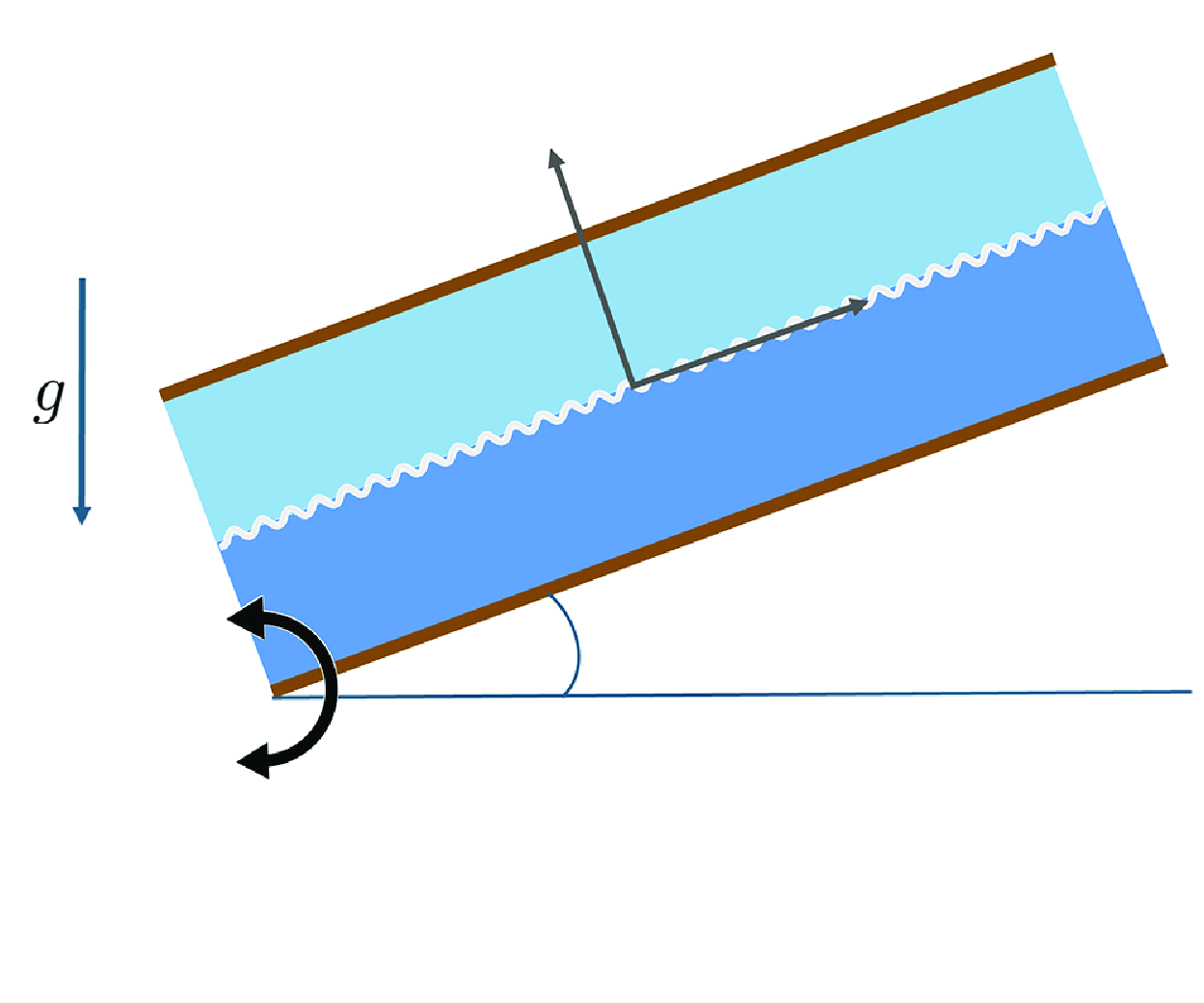
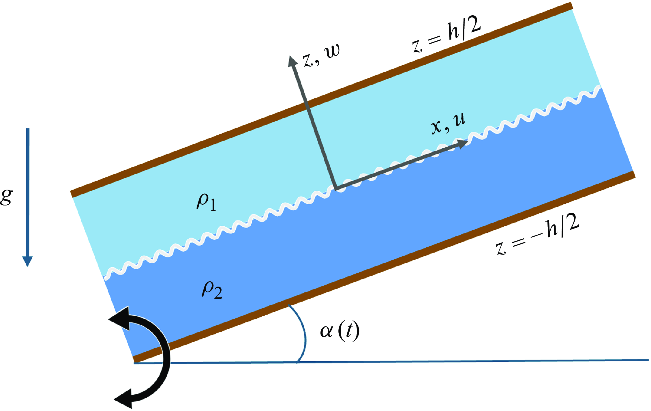
Schematic diagram of a two-layered oscillating tank, which can render short interfacial gravity waves unstable.
2.1. Background flow
We consider the two-dimensional (2-D) flow produced by oscillating a horizontal tank having a rectangular cross-section of depth $h$
, while the along-channel (
$h$
, while the along-channel ( $x$
) and cross-channel (
$x$
) and cross-channel ( $y$
) dimensions are infinite. The
$y$
) dimensions are infinite. The $z$
direction is positive upward; see figure 1 for the schematic of the set-up. The tank consists of a Boussinesq, two-layered, inviscid and immiscible fluid with the following density distribution:
$z$
direction is positive upward; see figure 1 for the schematic of the set-up. The tank consists of a Boussinesq, two-layered, inviscid and immiscible fluid with the following density distribution:
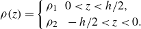 \begin{align} \rho (z) = \left \{ \begin{aligned} & \rho _1\,\,\, 0\lt z\lt h/2 ,\\ & \rho _2\,\,\, -h/2\lt z\lt 0. \end{aligned} \right . \end{align}
The fluid is stably stratified, i.e. $\rho _1\,{\lt}\,\rho _2$
. A more generic setting in which the two layers have unequal depths is discussed in Appendix A. Throughout the paper, subscripts
$\rho _1\,{\lt}\,\rho _2$
. A more generic setting in which the two layers have unequal depths is discussed in Appendix A. Throughout the paper, subscripts $1$
and
$1$
and $2$
will respectively denote quantities associated with the upper and lower fluid layers. The system is restricted to a small angle of oscillation
$2$
will respectively denote quantities associated with the upper and lower fluid layers. The system is restricted to a small angle of oscillation $\alpha (t)$
, typically
$\alpha (t)$
, typically $\textrm{max}\, |\alpha (t)|\lesssim 7^\circ$
. The small tilt of the density interface functions as a geophysically plausible mechanism for generating shear; the vertical motions induced by the sloping interface have a negligible effect on the fluid dynamics (Lewin & Caulfield Reference Lewin and Caulfield2022). For the setting in figure 1, the governing Navier–Stokes equations under the Boussinesq approximation read (Inoue & Smyth Reference Inoue and Smyth2009; Lewin & Caulfield Reference Lewin and Caulfield2022)
$\textrm{max}\, |\alpha (t)|\lesssim 7^\circ$
. The small tilt of the density interface functions as a geophysically plausible mechanism for generating shear; the vertical motions induced by the sloping interface have a negligible effect on the fluid dynamics (Lewin & Caulfield Reference Lewin and Caulfield2022). For the setting in figure 1, the governing Navier–Stokes equations under the Boussinesq approximation read (Inoue & Smyth Reference Inoue and Smyth2009; Lewin & Caulfield Reference Lewin and Caulfield2022)
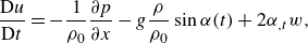 \begin{align} \frac {\mathrm{D}u}{\mathrm{D}t} = -\frac {1}{\rho _0}\frac {\partial p}{\partial x} - g\frac {\rho }{\rho _0}\sin \alpha (t) + 2 \alpha _{,t} w, \end{align}
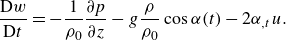 \begin{align} \frac {\mathrm{D}w}{\mathrm{D}t} = -\frac {1}{\rho _0}\frac {\partial p}{\partial z} - g\frac {\rho }{\rho _0}\cos \alpha (t) - 2 \alpha _{,t} u . \end{align}
Here, $\mathrm{D}/\mathrm{D}t = \partial /\partial t+\boldsymbol{u\cdot \nabla}$
, where
$\mathrm{D}/\mathrm{D}t = \partial /\partial t+\boldsymbol{u\cdot \nabla}$
, where $\boldsymbol{\nabla} =(\hat {\boldsymbol{x}}\,\partial /\partial x,\,\hat {\boldsymbol{z}}\,\partial /\partial z)$
,
$\boldsymbol{\nabla} =(\hat {\boldsymbol{x}}\,\partial /\partial x,\,\hat {\boldsymbol{z}}\,\partial /\partial z)$
, $\boldsymbol{u} = (u,\, w )$
is the velocity vector,
$\boldsymbol{u} = (u,\, w )$
is the velocity vector, $\rho _0$
is the constant reference density,
$\rho _0$
is the constant reference density, $g$
is the acceleration due to gravity and the suffix, ‘
$g$
is the acceleration due to gravity and the suffix, ‘ $_{,t}$
’ denotes ordinary derivative
$_{,t}$
’ denotes ordinary derivative ${\rm d}/{\rm d}t$
. The last terms in (2.2a
)–(2.2b
) represent Coriolis accelerations arising from the time-dependent rotation. The incompressibility condition is satisfied by the continuity equation
${\rm d}/{\rm d}t$
. The last terms in (2.2a
)–(2.2b
) represent Coriolis accelerations arising from the time-dependent rotation. The incompressibility condition is satisfied by the continuity equation
 \begin{equation} \frac {\partial u}{\partial x}+\frac {\partial w}{\partial z}=0. \end{equation}
The background state velocity is assumed to be parallel to the $x$
-axis, i.e.
$x$
-axis, i.e. $\boldsymbol{U}=(U,0)$
. Hence, the continuity equation, (2.3), implies that
$\boldsymbol{U}=(U,0)$
. Hence, the continuity equation, (2.3), implies that $U$
is only a function of
$U$
is only a function of $z$
and
$z$
and $t$
. Therefore, the background state equations yield
$t$
. Therefore, the background state equations yield
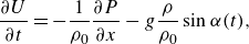 \begin{align} \frac {\partial U}{\partial t} &= -\frac {1}{\rho _0}\frac {\partial P}{\partial x} - g\frac {\rho }{\rho _0}\sin \alpha (t), \end{align}
 \begin{align} P &= - \int \left [g \rho (z) \cos \alpha (t) + 2 \rho _0 \alpha _{,t} U(z, t)\right ] \mathrm{d}z + \mathcal{G}(x,t), \end{align}
where $P(x,z,t)$
denotes the background state pressure.
$P(x,z,t)$
denotes the background state pressure.
Equation (2.1) indicates that $\rho$
is a function of
$\rho$
is a function of $z$
only. Consequently from (2.4b
),
$z$
only. Consequently from (2.4b
), $P(x,z,t)$
can be expressed as the sum of a function that is dependent on
$P(x,z,t)$
can be expressed as the sum of a function that is dependent on $z$
and
$z$
and $t$
, and another function
$t$
, and another function $\mathcal{G}$
dependent on
$\mathcal{G}$
dependent on $x$
and
$x$
and $t$
. This implies
$t$
. This implies $\partial P/\partial x$
is a function of
$\partial P/\partial x$
is a function of $x$
and
$x$
and $t$
. However, as per (2.4a
), both
$t$
. However, as per (2.4a
), both $\partial U/\partial t$
and
$\partial U/\partial t$
and $ g({\rho }/{\rho _0})\sin \alpha (t)$
are functions of
$ g({\rho }/{\rho _0})\sin \alpha (t)$
are functions of $z$
and
$z$
and $t$
only. Therefore,
$t$
only. Therefore, $\partial P/\partial x$
must be a function of
$\partial P/\partial x$
must be a function of $t$
alone. Since the tank is enclosed and there is no net flux across the walls, we must have (Thorpe Reference Thorpe1969)
$t$
alone. Since the tank is enclosed and there is no net flux across the walls, we must have (Thorpe Reference Thorpe1969)
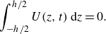 \begin{align} \int _{-h/2}^{h/2} U(z, t)\, \mathrm{d}z =0. \end{align}
The above condition can be used to obtain the background state velocity profile. In this regard, we integrate (2.4a
) in both $z$
and
$z$
and $t$
and substitute (2.5)
$t$
and substitute (2.5)
 \begin{equation} \int _0^t \frac {\partial P}{\partial x} \mathrm{d}t = -\frac {g}{h} \int _{-h/2}^{h/2} \rho \mathrm{d}z \int _0^t\sin \alpha (\tilde {t})\, \mathrm{d}\tilde {t}. \end{equation}
Finally, we integrate (2.4a
) in $t$
and combine with (2.6) and (2.1), which yields the background state velocity profile
$t$
and combine with (2.6) and (2.1), which yields the background state velocity profile
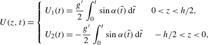 \begin{align} U(z,t) =\left \{ \begin{aligned} & U_1(t)=\frac {g^\prime }{2} \int _0^t \sin \alpha (\tilde {t}) \, \mathrm{d}\tilde {t} \,\,\,\,\,\,\,\,\, 0\lt z\lt h/2 ,\\ & U_2( t)=- \frac {g^\prime }{2} \int _0^t \sin \alpha (\tilde {t}) \, \mathrm{d}\tilde {t} \,\,\,\,\,\,-h/2\lt z\lt 0, \end{aligned} \right . \end{align}
where $g^\prime \,{=}\,{g}(\rho _2-\rho _1)/{\rho _0}$
is the reduced gravity. We assume that the tilt angle varies sinusoidally with time
$g^\prime \,{=}\,{g}(\rho _2-\rho _1)/{\rho _0}$
is the reduced gravity. We assume that the tilt angle varies sinusoidally with time
 \begin{align} \alpha (t)=\alpha _f\sin (\omega _f t), \end{align}
where $\alpha _f$
and
$\alpha _f$
and $\omega _f$
respectively denote the maximum angular amplitude and frequency of oscillation of the tilted tank. Since we have restricted our study to small oscillations (
$\omega _f$
respectively denote the maximum angular amplitude and frequency of oscillation of the tilted tank. Since we have restricted our study to small oscillations ( $\alpha _f\,{\ll}\,1$
), this implies
$\alpha _f\,{\ll}\,1$
), this implies $\sin \alpha \approx \alpha$
and
$\sin \alpha \approx \alpha$
and $\cos \alpha \approx 1-\alpha ^2/2$
. Under this assumption, the background state velocity in (2.7) simplifies to
$\cos \alpha \approx 1-\alpha ^2/2$
. Under this assumption, the background state velocity in (2.7) simplifies to
 \begin{align}&\quad U_1(t)= \frac {g^\prime }{2} \frac {\alpha _f}{\omega _f} [1-\cos (\omega _f t)]\quad 0\lt z\lt h/2 ,\end{align}
 \begin{align}& U_2(t) = - \frac {g^\prime }{2} \frac {\alpha _f}{\omega _f} [1-\cos (\omega _f t)] \quad -h/2\lt z\lt 0. \end{align}
The fact that the signs in (2.9a
)–(2.9b
) agree with our intuition can be verified by simply inspecting figure 1, which can be regarded as the maximum angle in the counter-clockwise direction attained by the tank, equalling $\alpha _f$
. As per (2.8) this implies
$\alpha _f$
. As per (2.8) this implies $\omega _f t\,{=}\,\pi /2$
, which, when substituted into (2.9a
)–(2.9b
), yields
$\omega _f t\,{=}\,\pi /2$
, which, when substituted into (2.9a
)–(2.9b
), yields $U_1\,{=}\,-U_2\,{=}\,g'\alpha _f/2\omega _f$
. The signs make sense because the heavier, lower layer must have a negative velocity since it would flow downwards due to gravity, and the upper layer should compensate for this by flowing upwards, yielding a positive velocity.
$U_1\,{=}\,-U_2\,{=}\,g'\alpha _f/2\omega _f$
. The signs make sense because the heavier, lower layer must have a negative velocity since it would flow downwards due to gravity, and the upper layer should compensate for this by flowing upwards, yielding a positive velocity.
2.2. Linear perturbations
We now consider the effect of infinitesimal perturbations added to the background state, and follow an approach similar to Thorpe (Reference Thorpe1969). The displacement of the two-fluid interface, given by $z\,{=}\,\xi (x,\,t)$
, sets up an irrotational perturbation velocity field in the two layers. The total velocity reads
$z\,{=}\,\xi (x,\,t)$
, sets up an irrotational perturbation velocity field in the two layers. The total velocity reads
 \begin{align} \boldsymbol{u}= \left \{ \begin{aligned} & U_1(t) \hat {\boldsymbol{x}} +\nabla \phi _1(x,z,t) \qquad 0 \lt z\lt h/2 ,\\ & U_2(t) \hat {\boldsymbol{x}} +\nabla \phi _2(x,z,t) \qquad -h/2\lt z\lt 0, \end{aligned} \right . \end{align}
where $\phi _{1}$
and
$\phi _{1}$
and $\phi _2$
are, respectively, the perturbation velocity potentials in the upper and lower fluid layers, which satisfy Laplace’s equation in their respective layers
$\phi _2$
are, respectively, the perturbation velocity potentials in the upper and lower fluid layers, which satisfy Laplace’s equation in their respective layers
 \begin{align} \boldsymbol{\nabla}^2 \phi _1&=0 \qquad\; 0 \lt z\lt h/2, \end{align}
 \begin{align} \boldsymbol{\nabla}^2 \phi _2&=0 \qquad -h/2\lt z\lt 0. \end{align}
The linearised dynamical boundary conditions at $z=0$
for the two layers are as follows:
$z=0$
for the two layers are as follows:
 \begin{align} \frac {P_1}{\rho _1}+\frac {\partial \phi _1}{\partial t} + \frac {\partial }{\partial t}\left (U_1 x\right ) + U_1 \frac {\partial \phi _1}{\partial x} + gx \sin \alpha (t) + gz\cos \alpha (t)=A_1(t), \end{align}
 \begin{align} \frac {P_2}{\rho _2}+\frac {\partial \phi _2}{\partial t} + \frac {\partial }{\partial t}\left (U_2 x\right ) + U_2 \frac {\partial \phi _2}{\partial x} + gx \sin \alpha (t)+ gz\cos \alpha (t) =A_2(t), \end{align}
where $P_1$
and
$P_1$
and $P_2$
, respectively, denote pressure in the upper and lower fluid layers, and
$P_2$
, respectively, denote pressure in the upper and lower fluid layers, and $A_1$
and
$A_1$
and $A_2$
are arbitrary functions of time. Likewise, the linearised kinematic boundary conditions at
$A_2$
are arbitrary functions of time. Likewise, the linearised kinematic boundary conditions at $z=0$
for the two layers read
$z=0$
for the two layers read
 \begin{align} \frac {\partial \xi }{\partial t} + U_1(t) \frac {\partial \xi }{\partial x} = \frac {\partial \phi _1}{\partial z},\\[-12pt]\nonumber \end{align}
 \begin{align} \frac {\partial \xi }{\partial t} + U_2(t) \frac {\partial \xi }{\partial x} = \frac {\partial \phi _2}{\partial z}. \end{align}
The upper and lower boundaries satisfy the impermeability condition
 \begin{align}&\,\, \frac {\partial \phi _1}{\partial z} = 0 \quad \text{at} \quad z=h/2, \end{align}
 \begin{align}& \frac {\partial \phi _2}{\partial z} = 0 \quad \text{at} \quad z=-h/2. \end{align}
Next, we assume the perturbations in the form of Fourier modes
 \begin{align} &\qquad\qquad\,\,\, \xi (x,t)= \eta (t) e^{\mathrm{i}kx}, \end{align}
 \begin{align} & \phi _1(x,z,t) =\psi _1(t)\cosh k\left (z-\frac {h}{2}\right )e^{\mathrm{i}kx}, \end{align}
 \begin{align} & \phi _2(x,z,t) =\psi _2(t)\cosh k\left (z+\frac {h}{2}\right )e^{\mathrm{i}kx}, \end{align}
where $k$
denotes the wavenumber and it is understood that the real parts of terms appearing on the right-hand sides are to be taken. It is straightforward to verify that the perturbation velocity potentials satisfy Laplace’s equations (2.11a
)–(2.11b
) and the impermeability condition (2.14a
)–(2.14b
). The continuity of pressure across the interface (
$k$
denotes the wavenumber and it is understood that the real parts of terms appearing on the right-hand sides are to be taken. It is straightforward to verify that the perturbation velocity potentials satisfy Laplace’s equations (2.11a
)–(2.11b
) and the impermeability condition (2.14a
)–(2.14b
). The continuity of pressure across the interface ( $P_1\,{=}\,P_2$
) is applied in (2.12a
)–(2.12b
), thereby combining these two equations into one
$P_1\,{=}\,P_2$
) is applied in (2.12a
)–(2.12b
), thereby combining these two equations into one
 \begin{align} \rho _1 A_1 &-\rho _1 \psi _{1,t} \cosh \left (\frac {kh}{2}\right ) e^{\mathrm{i}kx} - \rho _1 x U_{1,t} -\mathrm{i}k \rho _1 U_1 \psi _1 \cosh \left (\frac {kh}{2}\right ) e^{\mathrm{i}kx} - \rho _1 gx\sin \alpha (t) \nonumber \\ &- \rho _1 g \eta \cos \alpha (t) e^{\mathrm{i}kx} = \rho _2 A_2 -\rho _2 \psi _{2,t} \cosh \left (\frac {kh}{2}\right ) e^{\mathrm{i}kx} - \rho _2 x U_{2,t} \nonumber \\ &-\mathrm{i}k \rho _2 U_2 \psi _2 \cosh \left (\frac {kh}{2}\right ) e^{\mathrm{i}kx} - \rho _2 gx\sin \alpha (t) - \rho _2 g \eta \cos \alpha (t) e^{\mathrm{i}kx}. \end{align}
Note that, in the above equation, we have substituted (2.15a
)–(2.15c
). Next we collect the coefficients of $e^{\mathrm{i}kx}$
(Thorpe Reference Thorpe1969, Appendix A), and invoke the Boussinesq approximation
$e^{\mathrm{i}kx}$
(Thorpe Reference Thorpe1969, Appendix A), and invoke the Boussinesq approximation
 \begin{align} \left (\psi _{1,t}-\psi _{2,t}\right )\cosh \left (\frac {kh}{2}\right ) + \mathrm{i}k \left ( U_1 \psi _1 - U_2 \psi _2 \right )\cosh \left (\frac {kh}{2}\right ) = g' \eta \cos \alpha (t). \end{align}
Finally, we substitute the linearised kinematic boundary conditions (2.13a
)–(2.13b
) in the above equation, yielding a second-order ordinary differential equation (ODE) only in terms of $\eta$
 \begin{align} \eta _{,tt} +\Bigg[ \underbrace {\frac {kg^\prime }{2} \tanh \left (\frac {kh}{2}\right )}_{\text{$\omega ^2$}} \cos \alpha (t) -\frac {k^2}{2}\big(U_1(t)^2+U_2(t)^2\big)\Bigg] \eta =0. \end{align}
The explicit time dependence of the background flow has been intentionally emphasised. For a tank at rest, meaning $\alpha \,{=}\,0$
and
$\alpha \,{=}\,0$
and $U_1\,{=}\,U_2\,{=}\,0$
, we recover the equation governing interfacial gravity waves with frequency
$U_1\,{=}\,U_2\,{=}\,0$
, we recover the equation governing interfacial gravity waves with frequency $\omega =\pm \sqrt {(g'k/2)\tanh (kh/2)}$
propagating in a two-layered fluid where each layer has a depth of
$\omega =\pm \sqrt {(g'k/2)\tanh (kh/2)}$
propagating in a two-layered fluid where each layer has a depth of $h/2$
, see Sutherland (Reference Sutherland2010). Hereafter, we will restrict our attention to
$h/2$
, see Sutherland (Reference Sutherland2010). Hereafter, we will restrict our attention to $\tanh (kh/2 )\,{\approx}\,1$
, i.e. the waves are much shorter than the depth of the individual layers. The justification behind this choice is motivated by the fact that the wavelengths of KH instabilities arising in the pycnocline are usually much smaller than the pycnocline’s depth. Hence, the layer depths do not play any further role in governing the dynamics.
$\tanh (kh/2 )\,{\approx}\,1$
, i.e. the waves are much shorter than the depth of the individual layers. The justification behind this choice is motivated by the fact that the wavelengths of KH instabilities arising in the pycnocline are usually much smaller than the pycnocline’s depth. Hence, the layer depths do not play any further role in governing the dynamics.
Substituting (2.9a )–(2.9b ) into (2.18) yields
 \begin{align} \eta _{,tt} + \left [\! \omega ^{2} \!\left (\!1- \frac {\alpha _f^2}{4} (1-\cos (2\omega _ft))\!\right )\! - \omega ^{4}\frac {\alpha _f^2}{\omega _f^2} \!\left ( \frac {3}{2} - 2 \cos \left (\omega _ft\right ) + \frac {1}{2}\cos \left (2\omega _f t\right )\!\right )\!\right ]\eta =0. \end{align}
Hereafter, $\omega _f$
will represent low-frequency oscillations of the density interface. Physically, this can represent low-order, basin-scale modes (Sutherland Reference Sutherland2010, Chapter 2.5) which are essentially standing waves equivalent to seiches in lakes. Furthermore, although the analogy is tenuous,
$\omega _f$
will represent low-frequency oscillations of the density interface. Physically, this can represent low-order, basin-scale modes (Sutherland Reference Sutherland2010, Chapter 2.5) which are essentially standing waves equivalent to seiches in lakes. Furthermore, although the analogy is tenuous, $\omega _f$
can also represent the frequency of propagating long interfacial waves; see Inoue & Smyth (Reference Inoue and Smyth2009). In any case, the two-layered oscillating tank set-up in figure 1 is a simplified representation of the realistic scenario, and the key outcome in this context is the appearance of a small parameter
$\omega _f$
can also represent the frequency of propagating long interfacial waves; see Inoue & Smyth (Reference Inoue and Smyth2009). In any case, the two-layered oscillating tank set-up in figure 1 is a simplified representation of the realistic scenario, and the key outcome in this context is the appearance of a small parameter $\epsilon \,{=}\,\omega _f/\omega \,{\ll}\,1$
. In other words, the frequencies (wavelengths) of the gravity waves at the density interface, which could be rendered unstable, are orders of magnitude greater (smaller) than the frequencies (wavelengths) characterising the mean density interface, i.e. the background flow. The mean density interface represents a small-amplitude long wave of infinite wavelength, which essentially makes it a straight line and further ensures that the background shear flow is parallel.
$\epsilon \,{=}\,\omega _f/\omega \,{\ll}\,1$
. In other words, the frequencies (wavelengths) of the gravity waves at the density interface, which could be rendered unstable, are orders of magnitude greater (smaller) than the frequencies (wavelengths) characterising the mean density interface, i.e. the background flow. The mean density interface represents a small-amplitude long wave of infinite wavelength, which essentially makes it a straight line and further ensures that the background shear flow is parallel.
Defining a non-dimensional time $\tau \,{=}\,\omega _f t$
, (2.19) yields
$\tau \,{=}\,\omega _f t$
, (2.19) yields
 \begin{align} \epsilon ^2\eta _{,\tau \tau } + \Bigg[\underbrace {1- \frac {3}{2} \beta + \beta \left ( 2 \cos \left (\tau \right ) - \frac {1}{2}\cos \left (2\tau \right )\right ) }_{\text{$\mathcal{F}(\tau )$}}- \frac {\alpha _f^2}{4} \left (1-\cos (2\tau )\right ) \Bigg]\eta =0, \end{align}
where $\beta \,{=}\,\alpha _f^2/\epsilon ^2$
. Comparing
$\beta \,{=}\,\alpha _f^2/\epsilon ^2$
. Comparing $\beta$
with the definition of minimum Richardson number
$\beta$
with the definition of minimum Richardson number $Ri_{{min}}$
in Inoue & Smyth (Reference Inoue and Smyth2009), Equation (13), we observe that
$Ri_{{min}}$
in Inoue & Smyth (Reference Inoue and Smyth2009), Equation (13), we observe that $\beta$
resembles the inverse of minimum Richardson number. However, we are cautious that there is no length scale (shear layer thickness) in our problem, hence a direct comparison with Inoue & Smyth (Reference Inoue and Smyth2009) might be misleading. Note that
$\beta$
resembles the inverse of minimum Richardson number. However, we are cautious that there is no length scale (shear layer thickness) in our problem, hence a direct comparison with Inoue & Smyth (Reference Inoue and Smyth2009) might be misleading. Note that $\beta \,{\gg}\,\alpha _f^2$
, thus
$\beta \,{\gg}\,\alpha _f^2$
, thus $\mathcal{O}(\alpha _f^2)$
terms can be neglected. This transforms (2.20) into the following governing equation of the interface, which can be classified as a Schrödinger-type equation with a periodic potential:
$\mathcal{O}(\alpha _f^2)$
terms can be neglected. This transforms (2.20) into the following governing equation of the interface, which can be classified as a Schrödinger-type equation with a periodic potential:
 \begin{align} \epsilon ^2\eta _{,\tau \tau } + \mathcal{F}(\tau ) \eta =0 \quad \mathrm{where} \;\, \mathcal{F}(\tau )=\mathcal{F}(\tau +2\pi ). \end{align}
It is worthwhile to compare (2.21) with the governing ODE obtained by Kelly (Reference Kelly1965), Equation (3.17). Kelly’s two-layered flow with imposed layer-wise oscillating shear is only applicable to non-Boussinesq flows (shear disappears under the Boussinesq limit, see Kelly Reference Kelly1965, Equation (2.3)) and hence is fundamentally different from our system. The ODE governing Kelly’s system is Mathieu-type and therefore undergoes parametric instability when the forcing frequency $\omega _f$
is twice the natural frequency
$\omega _f$
is twice the natural frequency $\omega$
. Such parametric resonance is not expected to be the mechanism driving instability in our system since
$\omega$
. Such parametric resonance is not expected to be the mechanism driving instability in our system since $\omega$
and
$\omega$
and $\omega _f$
differ by many orders of magnitude. Furthermore, previous authors (Inoue & Smyth Reference Inoue and Smyth2009; Lewin & Caulfield Reference Lewin and Caulfield2022) do not report any finely tuned frequency ratios for observing the instability. The order separation of the two frequencies gives rise to the coefficient
$\omega _f$
differ by many orders of magnitude. Furthermore, previous authors (Inoue & Smyth Reference Inoue and Smyth2009; Lewin & Caulfield Reference Lewin and Caulfield2022) do not report any finely tuned frequency ratios for observing the instability. The order separation of the two frequencies gives rise to the coefficient $\epsilon ^2$
in the second derivative, thereby rendering (2.21) into a Schrödinger-type equation. We note in passing that Onuki, Joubaud & Dauxois (Reference Onuki, Joubaud and Dauxois2021) numerically studied the situation for which
$\epsilon ^2$
in the second derivative, thereby rendering (2.21) into a Schrödinger-type equation. We note in passing that Onuki, Joubaud & Dauxois (Reference Onuki, Joubaud and Dauxois2021) numerically studied the situation for which $\omega \,{\sim}\,\omega _f$
(hence
$\omega \,{\sim}\,\omega _f$
(hence $\epsilon \,{\sim}\,1$
), and indeed the authors report parametric subharmonic instability.
$\epsilon \,{\sim}\,1$
), and indeed the authors report parametric subharmonic instability.
2.2.1. Necessary and sufficient condition for instability
The nature of the solution to (2.21) is determined by the sign of $\mathcal{F}(\tau )$
; instability implies
$\mathcal{F}(\tau )$
; instability implies $\mathcal{F}(\tau )\,{\lt}\,0$
while the flow is stable for
$\mathcal{F}(\tau )\,{\lt}\,0$
while the flow is stable for $\mathcal{F}(\tau )\,{\gt}\,0$
. After some algebra, the necessary and sufficient condition for instability is found to be
$\mathcal{F}(\tau )\,{\gt}\,0$
. After some algebra, the necessary and sufficient condition for instability is found to be
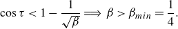 \begin{align} \cos \tau \lt 1-\frac {1}{\sqrt {\beta }}\,{\implies}\,\beta \gt \beta _{{min}} = \frac {1}{4}. \end{align}
This implies all waves with wavenumbers $k\gt k_{{long\hbox{-}wave\hbox{-}cut\hbox{-}off}}=\omega _f^2/2g'\alpha _f^2$
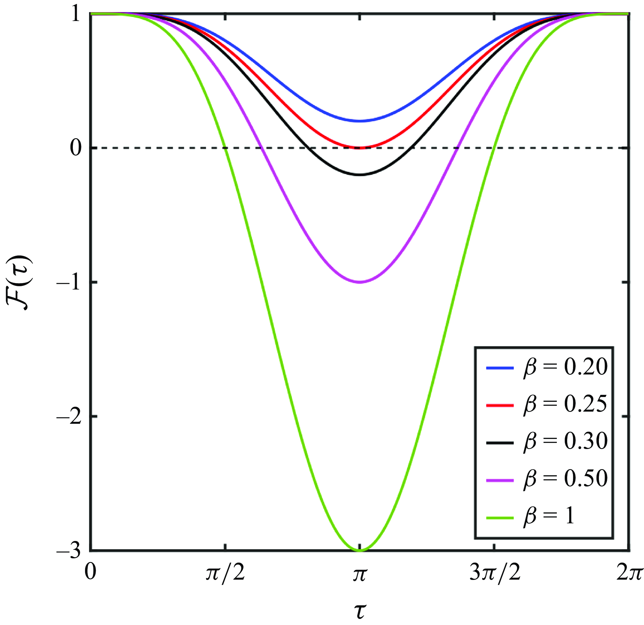
are unstable. Figure 2 represents the variation of
$k\gt k_{{long\hbox{-}wave\hbox{-}cut\hbox{-}off}}=\omega _f^2/2g'\alpha _f^2$
are unstable. Figure 2 represents the variation of $\mathcal{F}(\tau )$
with
$\mathcal{F}(\tau )$
with $\tau$
for various
$\tau$
for various $\beta$
values. Initially, the flow is stable for all finite
$\beta$
values. Initially, the flow is stable for all finite $\beta$
values. For
$\beta$
values. For $\beta \,{\gt}\,0.25$
, the solution ‘tunnels’ into the unstable region after crossing the (first) turning point
$\beta \,{\gt}\,0.25$
, the solution ‘tunnels’ into the unstable region after crossing the (first) turning point $\tau =\tau _c$
, which signifies
$\tau =\tau _c$
, which signifies $\mathcal{F}(\tau )$
changing sign from positive to negative. From (2.22),
$\mathcal{F}(\tau )$
changing sign from positive to negative. From (2.22), $\tau _c$
can be straightforwardly determined
$\tau _c$
can be straightforwardly determined
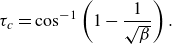 \begin{align} \tau _c = \cos ^{-1} \left (1-\frac {1}{\sqrt {\beta }}\right ). \end{align}
Noting that $\mathcal{F}(\tau )$
has a period of
$\mathcal{F}(\tau )$
has a period of $2\pi$
and a mirror symmetry about
$2\pi$
and a mirror symmetry about $\tau =\pi$
, it changes sign (for
$\tau =\pi$
, it changes sign (for $\beta \,{\gt}\,0.25$
) twice within its period – first at
$\beta \,{\gt}\,0.25$
) twice within its period – first at $\tau =\tau _c$
and then at
$\tau =\tau _c$
and then at $\tau =2\pi -\tau _c$
. The stability condition provides an upper bound for the time of occurrence of the instability – if the flow is unstable, then instability will set in before
$\tau =2\pi -\tau _c$
. The stability condition provides an upper bound for the time of occurrence of the instability – if the flow is unstable, then instability will set in before $\tau =\pi$
. The second turning point at
$\tau =\pi$
. The second turning point at $\tau =2\pi -\tau _c$
signifies stabilisation, which may have little effect for higher
$\tau =2\pi -\tau _c$
signifies stabilisation, which may have little effect for higher $\beta$
values that allow sustained growth for a longer time interval (
$\beta$
values that allow sustained growth for a longer time interval ( $2\pi -2\tau _c$
). This is because
$2\pi -2\tau _c$
). This is because $\tau _c$
reduces as
$\tau _c$
reduces as $\beta$
increases. Hence, the role of
$\beta$
increases. Hence, the role of $\beta$
is analogous to that of the inverse of the Richardson number.
$\beta$
is analogous to that of the inverse of the Richardson number.
In Appendix A, we discuss the generic situation in which the two fluid layers have unequal depths: $h_1$
and
$h_1$
and $h_2\,{=}\,h-h_1$
. In this scenario, the necessary and sufficient condition for instability is given by (see (A5))
$h_2\,{=}\,h-h_1$
. In this scenario, the necessary and sufficient condition for instability is given by (see (A5))
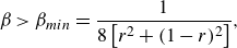 \begin{align} \beta \gt \beta _{{min}}= \frac {1}{8\left [r^2+(1-r)^2\right ]}, \end{align}
where $r=h_1/h$
. Since
$r=h_1/h$
. Since $r\in (0,1)$
, we must have
$r\in (0,1)$
, we must have $1/8\,{\lt}\,\beta _{{min}} \,{\leqslant}\, 1/4$
. The upper bound for the time of occurrence of the instability is independent of
$1/8\,{\lt}\,\beta _{{min}} \,{\leqslant}\, 1/4$
. The upper bound for the time of occurrence of the instability is independent of $r$
and occurs at
$r$
and occurs at $\tau \,{=}\,\pi$
. In the oceanographic context, the typical depth of the pycnocline (
$\tau \,{=}\,\pi$
. In the oceanographic context, the typical depth of the pycnocline ( $h_1$
) is much less than the total ocean depth (
$h_1$
) is much less than the total ocean depth ( $h$
), i.e.
$h$
), i.e. $r\,{\ll}\,1$
, which leads to the instability condition
$r\,{\ll}\,1$
, which leads to the instability condition $\beta \,{\gt}\,1/8$
.
$\beta \,{\gt}\,1/8$
.
Variation of $\mathcal{F}(\tau )$
with
$\mathcal{F}(\tau )$
with $\tau$
for different
$\tau$
for different $\beta$
values. The flow becomes unstable when
$\beta$
values. The flow becomes unstable when $\mathcal{F}(\tau )\lt 0$
. For reference,
$\mathcal{F}(\tau )\lt 0$
. For reference, $\tau \,{=}\,\pi /2$
implies the maximum counter-clockwise excursion (i.e.
$\tau \,{=}\,\pi /2$
implies the maximum counter-clockwise excursion (i.e. $\alpha =\alpha _f$
) of the two-layered oscillating tank, while
$\alpha =\alpha _f$
) of the two-layered oscillating tank, while $\tau \,{=}\,\pi$
implies that the tank, through clockwise rotation, has reached the horizontal position.
$\tau \,{=}\,\pi$
implies that the tank, through clockwise rotation, has reached the horizontal position.
2.2.2. Predictions from the steady background flow assumption
Undertaking a conventional, steady-state-based linear stability analysis for an inherently unsteady background flow could appear simplistic. However, such an analysis has a key advantage – the simplifications can result in an exact solution of (2.21), leading to a closed-form expression for the growth rate. Furthermore, if the growth is exponential (verified a posteriori), then the time scale of growth is much faster than the slow time dependence of the background flow, implying that the steady-state assumption is sensible. Here we intend to explore the predictions obtained from steady-state-based analyses and the extent of errors incurred.
One way of removing the explicit time dependence of the background flow is time averaging. By averaging (2.9a )–(2.9b ) over its period, we obtain
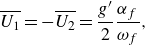 \begin{equation} \overline {U_1}=-\overline {U_2}=\frac {g^\prime }{2} \frac {\alpha _f}{\omega _f}, \end{equation}
which when substituted into (2.18) converts (2.21) into a second-order constant coefficient ODE with $\mathcal{F}=1-\beta$
. This yields the instability condition
$\mathcal{F}=1-\beta$
. This yields the instability condition $\beta \,{\gt}\,1$
, which implies normal-mode instabilities with a growth rate of
$\beta \,{\gt}\,1$
, which implies normal-mode instabilities with a growth rate of $\sigma _{{normal\hbox{-}mode}}\,{=}\,\sqrt {\beta -1}/\epsilon$
. Comparison with (2.22) shows that the above instability condition is erroneous.
$\sigma _{{normal\hbox{-}mode}}\,{=}\,\sqrt {\beta -1}/\epsilon$
. Comparison with (2.22) shows that the above instability condition is erroneous.
Next, we undertake another steady-state-based approach where the maximum background velocity of each layer given in (2.9a )–(2.9b ) is considered
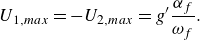 \begin{equation} U_{1,{max}}=- U_{2,{max}}=g^\prime \frac {\alpha _f}{\omega _f}. \end{equation}
The above background velocities are substituted in (2.18) yielding $\mathcal{F}=1-4\beta$
in the governing equation (2.21). This flow becomes unstable to normal-mode instabilities which has a growth rate of
$\mathcal{F}=1-4\beta$
in the governing equation (2.21). This flow becomes unstable to normal-mode instabilities which has a growth rate of
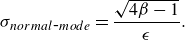 \begin{equation} \sigma _{{normal\hbox{-}mode}}=\frac {\sqrt {4\beta - 1}}{\epsilon }. \end{equation}
The resulting instability condition $\beta \,{\gt}\,1/4$
exactly matches the unsteady analysis in (2.22). To see how this growth rate compares with the classical KH instability of two discontinuous layers, we write the well-known expression for its dimensional growth rate (Drazin & Reid Reference Drazin and Reid2004; Guha & Rahmani Reference Guha and Rahmani2019)
$\beta \,{\gt}\,1/4$
exactly matches the unsteady analysis in (2.22). To see how this growth rate compares with the classical KH instability of two discontinuous layers, we write the well-known expression for its dimensional growth rate (Drazin & Reid Reference Drazin and Reid2004; Guha & Rahmani Reference Guha and Rahmani2019)
 \begin{equation} \widetilde {\sigma }_{\textit{KH}}\,{=}\,\sqrt {U^2k^2-\frac {g'k}{2}}, \end{equation}
where the upper (lower) layer of density $\rho _1\,(\rho _2)$
is moving with a constant velocity
$\rho _1\,(\rho _2)$
is moving with a constant velocity $U\,(- U)$
. Substituting
$U\,(- U)$
. Substituting $U\,{=}\,U_{1,{max}}$
from (2.26) and non-dimensionalising (2.28) with
$U\,{=}\,U_{1,{max}}$
from (2.26) and non-dimensionalising (2.28) with $\omega _f$
, it is straightforward to verify that the non-dimensional growth rate
$\omega _f$
, it is straightforward to verify that the non-dimensional growth rate ${\sigma }_{\textit{KH}}\,{=}\,{\widetilde {\sigma }_{\textit{KH}}}/{\omega _f}\,{=}\,\sigma _{{normal\hbox{-}mode}}$
in (2.27).
${\sigma }_{\textit{KH}}\,{=}\,{\widetilde {\sigma }_{\textit{KH}}}/{\omega _f}\,{=}\,\sigma _{{normal\hbox{-}mode}}$
in (2.27).
In summary, the steady-state-based linear stability analysis that considers the maximum (instead of time-average) background velocity in each layer provides the same instability condition as the time-dependent problem. The normal-mode growth rate exactly matches the classical KH instability. However, such an analysis is unable to capture key features of the actual system, which is inherently unsteady. For example, the steady-state-based analysis cannot predict the time of onset of the instability. Since $\tau$
is a slow time, a delayed onset of instability is a salient feature of this system. How well the growth rate predicted from the steady-state-based analysis compares with the unsteady analysis also needs to be examined.
$\tau$
is a slow time, a delayed onset of instability is a salient feature of this system. How well the growth rate predicted from the steady-state-based analysis compares with the unsteady analysis also needs to be examined.
3. Linear stability analysis
3.1. Floquet analysis, numerical integration and normal-mode predictions
Equation (2.21) can be written as a 2-D dynamical system
 \begin{equation} \begin{bmatrix} \eta \\ v \end{bmatrix}_{,\tau } =\underbrace {\begin{bmatrix} 0 & 1 \\ -{\epsilon ^{-2}}\mathcal{F}(\tau ) & 0 \end{bmatrix}}_{\text{$\mathcal{L}(\tau )$}} \begin{bmatrix} \eta \\ v \end{bmatrix}, \end{equation}
where the linear operator $\mathcal{L}(\tau )$
has a fundamental period of
$\mathcal{L}(\tau )$
has a fundamental period of $T\,{=}\,2\pi$
. The fundamental solution matrix
$T\,{=}\,2\pi$
. The fundamental solution matrix $\Phi (\tau )$
satisfies
$\Phi (\tau )$
satisfies
 \begin{align} \Phi _{,\tau }(\tau ) = \mathcal{L}(\tau )\Phi (\tau ) \quad \text{where} \;\, \Phi (0)=I. \end{align}
Floquet analysis is the standard technique for analysing the stability of linear periodic systems. If the analysis finds that the energy of the disturbance at the end of one period is larger than the energy at the outset, the system is deemed unstable. In this regard, the monodromy matrix $\Phi (T)$
(which is numerically computed in general) is first determined and its eigenvalues, known as Floquet multipliers
$\Phi (T)$
(which is numerically computed in general) is first determined and its eigenvalues, known as Floquet multipliers $\mu$
, are sought. The Floquet exponents
$\mu$
, are sought. The Floquet exponents $\Omega$
, signifying the complex temporal growth rate, are related to the Floquet multipliers via the relation
$\Omega$
, signifying the complex temporal growth rate, are related to the Floquet multipliers via the relation $\mu \,{=}\,\exp {(\Omega T)}$
. The system is deemed unstable if there exists at least one eigenvalue satisfying
$\mu \,{=}\,\exp {(\Omega T)}$
. The system is deemed unstable if there exists at least one eigenvalue satisfying $|\mu |\,{\gt}\,1$
(
$|\mu |\,{\gt}\,1$
( $\mathrm{Re}(\Omega )\,{\gt}\,0$
). Likewise, the system is stable if all eigenvalues satisfy
$\mathrm{Re}(\Omega )\,{\gt}\,0$
). Likewise, the system is stable if all eigenvalues satisfy $|\mu |\,{\lt}\,1$
(
$|\mu |\,{\lt}\,1$
( $\mathrm{Re}(\Omega )\,{\lt}\,0$
). When all eigenvalues satisfy
$\mathrm{Re}(\Omega )\,{\lt}\,0$
). When all eigenvalues satisfy $|\mu |\,{=}\,1$
(
$|\mu |\,{=}\,1$
( $\mathrm{Re}(\Omega )\,{=}\,0$
), the system oscillates between finite bounds
$\mathrm{Re}(\Omega )\,{=}\,0$
), the system oscillates between finite bounds $\forall \tau$
(Richards Reference Richards2002). In this case, the solution is neutrally stable and can yield quasiperiodic behaviour in time (Kovacic, Rand & Mohamed Sah Reference Kovacic, Rand and Mohamed Sah2018).
$\forall \tau$
(Richards Reference Richards2002). In this case, the solution is neutrally stable and can yield quasiperiodic behaviour in time (Kovacic, Rand & Mohamed Sah Reference Kovacic, Rand and Mohamed Sah2018).
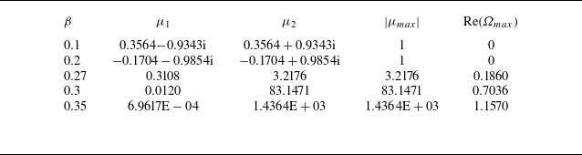
We compute Floquet exponents and the Floquet multipliers using Matlab corresponding to different $\beta$
values in table 1. We keep
$\beta$
values in table 1. We keep $\alpha _f$
fixed at
$\alpha _f$
fixed at $0.05$
(which is equivalent to
$0.05$
(which is equivalent to $2.86$
°) in the entire paper. The system is bounded for
$2.86$
°) in the entire paper. The system is bounded for $\beta \,{=}\,0.1$
and
$\beta \,{=}\,0.1$
and $0.2$
, and unstable for
$0.2$
, and unstable for $0.27$
,
$0.27$
, $0.3$
and
$0.3$
and $0.35$
, which are the expected outcomes as per the condition in (2.22). Furthermore, we also observe that, when
$0.35$
, which are the expected outcomes as per the condition in (2.22). Furthermore, we also observe that, when $\beta \,{\gt}\,0.25$
, the higher the
$\beta \,{\gt}\,0.25$
, the higher the $\beta$
value, the higher the maximum growth rate
$\beta$
value, the higher the maximum growth rate $\mathrm{Re}(\Omega _{{max}})$
. We restrict our Floquet analysis to up to
$\mathrm{Re}(\Omega _{{max}})$
. We restrict our Floquet analysis to up to $\beta \,{=}\,0.35$
since, beyond this value, the numerical solution becomes unreliable owing to the resulting extremely large and extremely small Floquet multipliers.
$\beta \,{=}\,0.35$
since, beyond this value, the numerical solution becomes unreliable owing to the resulting extremely large and extremely small Floquet multipliers.
Floquet analysis of the system (3.1).
To understand how the amplitude evolves in time, and to explore a bigger range of $\beta$
values, we numerically solve (2.21) using Matlab’s inbuilt ODE45 solver (which was also used to construct the monodromy matrix while performing the Floquet analysis). For the two initial conditions, we take
$\beta$
values, we numerically solve (2.21) using Matlab’s inbuilt ODE45 solver (which was also used to construct the monodromy matrix while performing the Floquet analysis). For the two initial conditions, we take
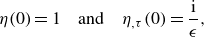 \begin{align} \eta (0)=1 \quad \text{and} \quad \eta _{,\tau }(0) =\frac {\mathrm{i}}{\epsilon }, \end{align}
which satisfy the governing equation
 \begin{align} \epsilon ^2 \eta _{,\tau \tau } + \eta =0. \end{align}
The above equation, which can be obtained by taking the limit $\tau \rightarrow 0$
of (2.21), physically represents propagating deep water interfacial waves inside the two-layered horizontal tank at rest (i.e. non-oscillating).
$\tau \rightarrow 0$
of (2.21), physically represents propagating deep water interfacial waves inside the two-layered horizontal tank at rest (i.e. non-oscillating).
Plots of $|\eta |$
vs
$|\eta |$
vs $\tau$
for different
$\tau$
for different $\beta$
values. Unstable regions predicted from (2.23) are shaded in grey. Line colours are as follows: black – normal-mode solution (based on steady background flow (2.26)), blue – numerical solution of (2.21) and dashed red – MAF solution (3.21). The dashed-blue line in (b) represents the amplitude envelope.
$\beta$
values. Unstable regions predicted from (2.23) are shaded in grey. Line colours are as follows: black – normal-mode solution (based on steady background flow (2.26)), blue – numerical solution of (2.21) and dashed red – MAF solution (3.21). The dashed-blue line in (b) represents the amplitude envelope.
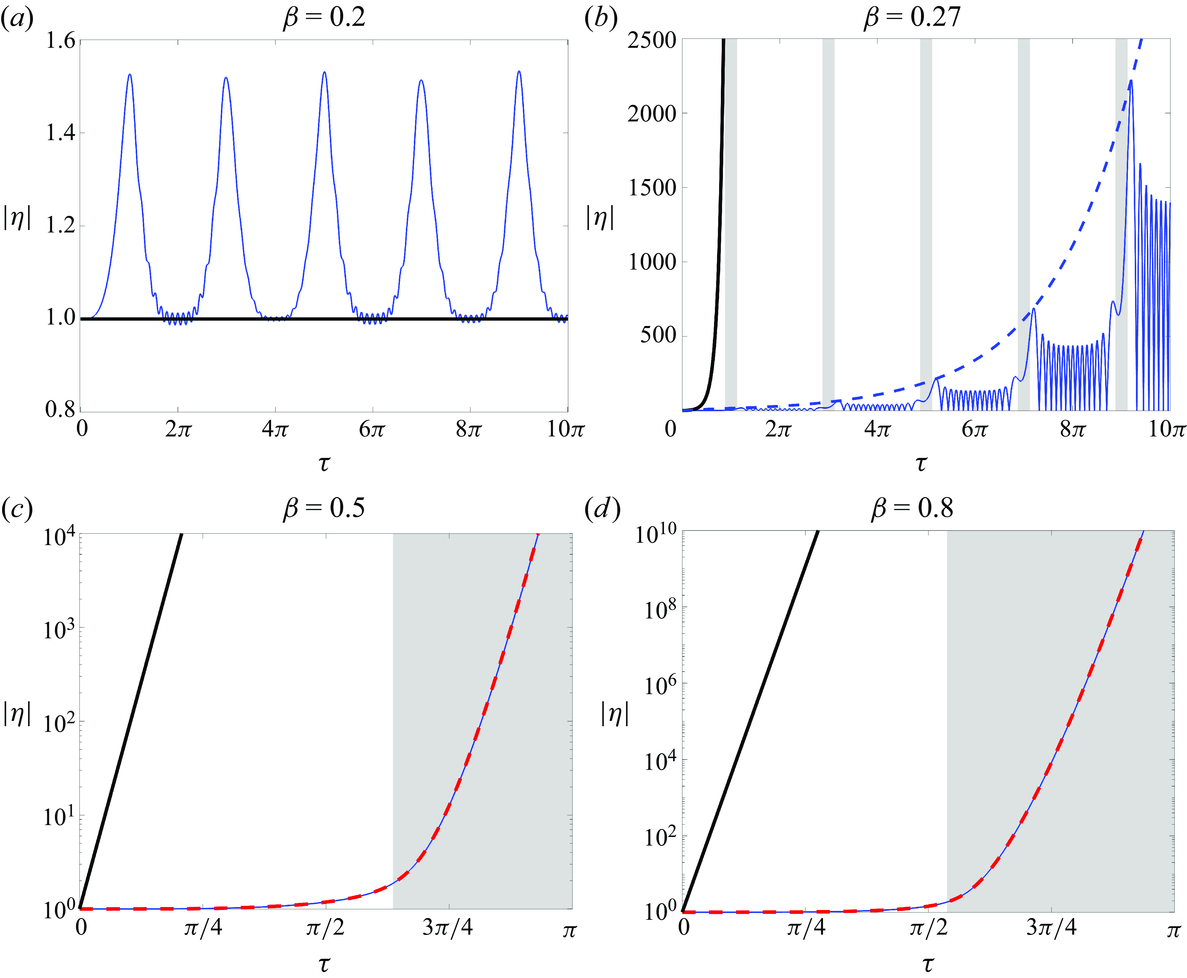
Figure 3(a) shows that the system undergoes bounded oscillations for $\beta \,{=}\,0.2$
, which cannot be predicted from the normal-mode theory. As already noted in § 2.2, systems with
$\beta \,{=}\,0.2$
, which cannot be predicted from the normal-mode theory. As already noted in § 2.2, systems with $\beta \,{\gt}\,0.25$
start becoming unstable when
$\beta \,{\gt}\,0.25$
start becoming unstable when $\tau \,{\gt}\,\tau _c$
. Within the
$\tau \,{\gt}\,\tau _c$
. Within the $n$
th period, the system will grow when
$n$
th period, the system will grow when $2n\pi +\tau _c \,{\lt}\,\tau \,{\lt}\,2(n+1)\pi -\tau _c$
, i.e. the interval when
$2n\pi +\tau _c \,{\lt}\,\tau \,{\lt}\,2(n+1)\pi -\tau _c$
, i.e. the interval when $\mathcal{F}(\tau )\,{\lt}\,0$
is satisfied. This fact is evident in figure 3(b) which corresponds to
$\mathcal{F}(\tau )\,{\lt}\,0$
is satisfied. This fact is evident in figure 3(b) which corresponds to $\beta \,{=}\,0.27$
. Furthermore, the plot also reveals the amplification of energy between consecutive periods. Figures 3(c) and 3(d) respectively correspond to
$\beta \,{=}\,0.27$
. Furthermore, the plot also reveals the amplification of energy between consecutive periods. Figures 3(c) and 3(d) respectively correspond to $\beta \,{=}\,0.5$
and
$\beta \,{=}\,0.5$
and $\beta \,{=}\,0.8$
, and reveal a much larger growth rate, as is expected from the trend observed in table 1.
$\beta \,{=}\,0.8$
, and reveal a much larger growth rate, as is expected from the trend observed in table 1.
Finally, we compare the growth rate $\sigma _{{numerical}}$
obtained from the numerical solutions (calculated when
$\sigma _{{numerical}}$
obtained from the numerical solutions (calculated when $\tau \,{\gt}\,\tau _c$
) with the normal-mode predictions in (2.27):
$\tau \,{\gt}\,\tau _c$
) with the normal-mode predictions in (2.27):
-
(i) $\beta \,{=}\,0.27$
:
$\sigma _{{normal\hbox{-}mode}}=2.94\;\,\kern-1pt$
$\sigma _{{numerical}}=0.18$
(amplitude envelope growth rate);
$\beta \,{=}\,0.27$
:
$\sigma _{{normal\hbox{-}mode}}=2.94\;\,\kern-1pt$
$\sigma _{{numerical}}=0.18$
(amplitude envelope growth rate); -
(ii)
$\beta \,{=}\,0.5$
:
$\sigma _{{normal\hbox{-}mode}}=14.14$
$\sigma _{{numerical}}=14.12$
; -
(iii)
$\beta \,{=}\,0.8$
:
$\!\sigma _{{normal\hbox{-}mode}}=26.53$
$\sigma _{{numerical}}=26.53$
.


As evident from the above data and also from figures 3(c) and 3(d), the normal-mode growth rate predictions from (2.27) provide an excellent agreement with the numerical solution, and this agreement improves even further as $\beta$
increases. Since the normal-mode growth rate exactly matches with that of the classical KH instability, this conclusively proves that the instability is of KH type. However, for the
$\beta$
increases. Since the normal-mode growth rate exactly matches with that of the classical KH instability, this conclusively proves that the instability is of KH type. However, for the $\beta \,{=}\,0.27$
(which is a
$\beta \,{=}\,0.27$
(which is a $\beta$
value slightly greater than the instability condition) case, the normal-mode theory fails to predict the growth rate of the amplitude envelope, as well as the intricate temporal dynamics of the amplitude evolution, which is clear from figure 3(b).
$\beta$
value slightly greater than the instability condition) case, the normal-mode theory fails to predict the growth rate of the amplitude envelope, as well as the intricate temporal dynamics of the amplitude evolution, which is clear from figure 3(b).
We also emphasise here that $\beta$
, by definition, is proportional to
$\beta$
, by definition, is proportional to $\omega ^2\,{=}\,g'k/2$
. The growth rate trend reveals the classical ‘ultraviolet catastrophe’, i.e. shorter waves are more unstable, which is an artefact of the absence of a length scale (i.e. finite thickness of the interface) in the problem.
$\omega ^2\,{=}\,g'k/2$
. The growth rate trend reveals the classical ‘ultraviolet catastrophe’, i.e. shorter waves are more unstable, which is an artefact of the absence of a length scale (i.e. finite thickness of the interface) in the problem.
Finally, we compare our theoretical predictions with the DNS results of Lewin & Caulfield (Reference Lewin and Caulfield2022). In this regard, we choose the case ‘NM72D’, where normal-mode perturbations have been used to seed the flow. Note that the authors use smooth profiles, hence, their parameters need to be suitably adjusted to fit our discontinuous set-up. Their parameters are as follows: $\alpha _f\,{=}\,7.28^\circ \,{=}\,0.127$
radians,
$\alpha _f\,{=}\,7.28^\circ \,{=}\,0.127$
radians, $\lambda \,{=}\,14.28$
implying
$\lambda \,{=}\,14.28$
implying $k\,{=}\,0.44$
, half-shear layer thickness
$k\,{=}\,0.44$
, half-shear layer thickness $\delta \,{=}\,1$
and
$\delta \,{=}\,1$
and $\omega _f/N_b\,{=}\,0.072$
, where
$\omega _f/N_b\,{=}\,0.072$
, where $N_b$
denotes background buoyancy frequency. Noting that
$N_b$
denotes background buoyancy frequency. Noting that $g'\,{=}\, N_b^2\delta$
, we can state
$g'\,{=}\, N_b^2\delta$
, we can state $\epsilon ^2$
in their variables
$\epsilon ^2$
in their variables
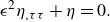
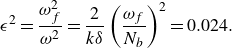 \begin{align} \epsilon ^2=\frac {\omega _f^2}{\omega ^2}=\frac {2}{k\delta }\left (\frac {\omega _f}{N_b}\right )^2=0.024. \end{align}
This yields
 \begin{align} \beta =\frac {\alpha _f^2}{\epsilon ^2}=0.67\gt \frac {1}{4}, \end{align}
and thus the set-up for NM72D satisfies our instability condition (2.22). Indeed, the authors observe KH instability for the case NM72D. Furthermore, the onset of instability predicted from (2.23) is $\tau _c\,{=}\,0.57\pi$
, which excellently matches the corresponding DNS result
$\tau _c\,{=}\,0.57\pi$
, which excellently matches the corresponding DNS result $\tau _c\,{=}\,0.54\pi$
(see the Acknowledgement). However, we provide a note of caution that while certain instability characteristics (e.g.
$\tau _c\,{=}\,0.54\pi$
(see the Acknowledgement). However, we provide a note of caution that while certain instability characteristics (e.g. $\tau _c$
) can have a direct quantitative agreement between discontinuous and smooth profiles, this does not guarantee a correspondence between other instability characteristics. For example, growth rates obtained from discontinuous profiles are unreliable. Moreover, discontinuous profiles cannot predict the band of unstable wavenumbers or the most unstable wavenumber. A proper evaluation of these parameters demands consideration of a finite-thickness shear layer.
$\tau _c$
) can have a direct quantitative agreement between discontinuous and smooth profiles, this does not guarantee a correspondence between other instability characteristics. For example, growth rates obtained from discontinuous profiles are unreliable. Moreover, discontinuous profiles cannot predict the band of unstable wavenumbers or the most unstable wavenumber. A proper evaluation of these parameters demands consideration of a finite-thickness shear layer.
3.2. Asymptotic solution: the modified Airy function method
Here, we aim to construct an approximate solution to the amplitude evolution. A standard approach in this regard would be to employ the well-known singular perturbation technique – the Wentzel–Kramers–Brillouin (WKB) method (Bender & Orszag Reference Bender and Orszag2013). In the WKB method, the asymptotic series in the small parameter $\epsilon$
is written as follows:
$\epsilon$
is written as follows:
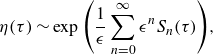 \begin{align} \eta (\tau ) \sim \exp {\left (\frac {1}{\epsilon } \sum \limits _{n=0}^{\infty } \epsilon ^n S_n(\tau )\right )}, \end{align}
where $S_n(\tau )$
denotes the complex phase. Substitution of the above expansion in (2.21) yields the following first-order expressions for
$S_n(\tau )$
denotes the complex phase. Substitution of the above expansion in (2.21) yields the following first-order expressions for $\eta$
(valid for
$\eta$
(valid for $0\,{\leqslant}\,\tau \,{\lt}\, 2\pi -\tau _c$
, i.e. up to the second turning point:
$0\,{\leqslant}\,\tau \,{\lt}\, 2\pi -\tau _c$
, i.e. up to the second turning point:
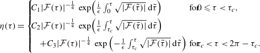 \begin{equation} \eta (\tau ) = \left \{ \!\!\begin{array}{lll} C_1|\mathcal{F}(\tau )|^{-\frac {1}{4}} \,\exp \!\left (\frac {\mathrm{i}}{\epsilon } \int _{0}^{\tau } \sqrt {|\mathcal{F}(\tilde {\tau })|}\,\mathrm{d}\tilde {\tau }\right ) &\text{for} &\!\!\kern-1pt 0\,{\leqslant}\,\tau \,{\lt}\,\tau _c,\\[6pt] C_2|\mathcal{F}(\tau )|^{-\frac {1}{4}} \,\exp \!\left (\frac {1}{\epsilon } \int _{\tau _c}^\tau \sqrt {|\mathcal{F}(\tilde {\tau })|}\,\mathrm{d}\tilde {\tau }\right ) \\[6pt] \quad +C_3|\mathcal{F}(\tau )|^{-\frac {1}{4}} \,\exp \left (-\frac {1}{\epsilon } \int _{\tau _c}^\tau \sqrt {|\mathcal{F}(\tilde {\tau })|}\,\mathrm{d}\tilde {\tau }\right ) & \text{for} &\!\!\! \tau _c\,{\lt}\,\tau \,{\lt}\,2\pi -\tau _c. \end{array} \right . \end{equation}
The solution exhibits an oscillatory behaviour when $\tau \,{\lt}\,\tau _c$
and grows monotonically (the decaying solution would rapidly become insignificant) when
$\tau \,{\lt}\,\tau _c$
and grows monotonically (the decaying solution would rapidly become insignificant) when $\tau _c\,{\lt}\,\tau \,{\lt}\,2\pi -\tau _c$
. Note that
$\tau _c\,{\lt}\,\tau \,{\lt}\,2\pi -\tau _c$
. Note that $C_1$
can be straightforwardly determined from (3.3) and yields
$C_1$
can be straightforwardly determined from (3.3) and yields $C_1\,{=}\,1$
. To find
$C_1\,{=}\,1$
. To find $C_2$
and
$C_2$
and $C_3$
, turning point analysis at
$C_3$
, turning point analysis at $\tau \,{=}\,\tau _c$
is required, which employs Airy functions to match the solutions on the two sides of the turning point. Instead of the standard WKB turning point analysis, we employ the modified Airy function (MAF) method, which can be regarded as an improved variant of WKB. The key aspect of MAF is its recognition of the fact that the Airy functions provide a uniformly valid composite approximation both near and far from a turning point. The MAF method was first introduced by Langer (Reference Langer1935); for a detailed discussion on this technique, also see Ghatak, Gallawa & Goyal (Reference Ghatak, Gallawa and Goyal1991), Bender & Orszag (Reference Bender and Orszag2013) and Wine, Achtymichuk & Marsiglio (Reference Wine, Achtymichuk and Marsiglio2025). Here, we employ MAF to analyse both turning points, and hence obtain a uniformly valid solution for the entire period of
$\tau \,{=}\,\tau _c$
is required, which employs Airy functions to match the solutions on the two sides of the turning point. Instead of the standard WKB turning point analysis, we employ the modified Airy function (MAF) method, which can be regarded as an improved variant of WKB. The key aspect of MAF is its recognition of the fact that the Airy functions provide a uniformly valid composite approximation both near and far from a turning point. The MAF method was first introduced by Langer (Reference Langer1935); for a detailed discussion on this technique, also see Ghatak, Gallawa & Goyal (Reference Ghatak, Gallawa and Goyal1991), Bender & Orszag (Reference Bender and Orszag2013) and Wine, Achtymichuk & Marsiglio (Reference Wine, Achtymichuk and Marsiglio2025). Here, we employ MAF to analyse both turning points, and hence obtain a uniformly valid solution for the entire period of $2\pi$
. In MAF, the amplitude
$2\pi$
. In MAF, the amplitude $\eta (\tau )$
is expressed as
$\eta (\tau )$
is expressed as
 \begin{align} \eta (\tau ) =\left \{ \!\begin{aligned} & F_1(\tau ) Ai\left (\zeta _1(\tau )\right ) + G_1(\tau ) Bi\left (\zeta _1(\tau )\right ) \quad \mbox{for}\; 0\leqslant \tau \leqslant \tau _p, \\ &F_2(\tau ) Ai\left (\zeta _2(\tau )\right ) + G_2(\tau ) Bi\left (\zeta _2(\tau )\right ) \quad \mbox{for}\; \tau _p\leqslant \tau \leqslant 2\pi , \end{aligned} \right . \end{align}
where $\tau _p\,{=}\,\pi$
is the location of absolute minima of the periodic potential
$\tau _p\,{=}\,\pi$
is the location of absolute minima of the periodic potential $\mathcal{F}(\tau )$
, and
$\mathcal{F}(\tau )$
, and $Ai(\zeta )$
and
$Ai(\zeta )$
and $Bi(\zeta )$
, respectively, the MAFs of the first and second kinds, satisfy
$Bi(\zeta )$
, respectively, the MAFs of the first and second kinds, satisfy
 \begin{align} Ai_{,\zeta \zeta } - \zeta Ai(\zeta )=0, \quad \mbox{and} \quad Bi_{,\zeta \zeta } - \zeta Bi(\zeta )=0. \end{align}
We will proceed by focusing on one of the terms (say, $F_1(\tau ) Ai (\zeta _1(\tau ) )$
) in (3.9), as the other terms follow similar algebra, and they can be treated independently. Substituting
$F_1(\tau ) Ai (\zeta _1(\tau ) )$
) in (3.9), as the other terms follow similar algebra, and they can be treated independently. Substituting $F_1(\tau ) Ai (\zeta _1(\tau ) )$
into the governing equation (2.21) and using the Airy function equations we obtain
$F_1(\tau ) Ai (\zeta _1(\tau ) )$
into the governing equation (2.21) and using the Airy function equations we obtain
 \begin{align} F_{1,\tau \tau } Ai(\zeta ) +2 F_{1,\tau } Ai_{,\zeta _1} \zeta _{1,\tau } + F_1 Ai_{,\zeta _1} \zeta _{1,\tau \tau }+ F_1\, Ai(\zeta _1) \big[ \epsilon ^2 \zeta _1(\tau ) \zeta _{1,\tau }^2 + \mathcal{F}(\tau ) \big]=0. \end{align}
To eliminate the terms in square brackets, $\zeta _1(\tau )$
is chosen to satisfy
$\zeta _1(\tau )$
is chosen to satisfy
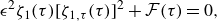 \begin{align} {\epsilon ^2} \zeta _1(\tau ) [\zeta _{1,\tau }(\tau )]^2 + {\mathcal{F}(\tau )}=0, \end{align}
which gives
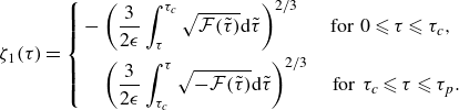 \begin{align} \zeta _1(\tau ) =\left \{ \begin{aligned} -&\left (\frac {3}{2\epsilon } \int _\tau ^{\tau _c} \sqrt {\mathcal{F}(\tilde {\tau })} \mathrm{d}\tilde {\tau } \right )^{2/3} \quad \;\;\kern1pt\text{for} \;\, 0 \leqslant \tau \leqslant \tau _c,\\ & \left (\frac {3}{2\epsilon } \int _{\tau _c}^{\tau } \sqrt {-\mathcal{F}(\tilde {\tau })} \mathrm{d}\tilde {\tau } \right )^{2/3} \quad \text{for} \;\, \tau _c \leqslant \tau \leqslant \tau _p. \end{aligned} \right . \end{align}
Here, $F_1(\tau )$
is obtained by assuming
$F_1(\tau )$
is obtained by assuming $F_{1,\tau \tau } \approx 0$
. Thus,
$F_{1,\tau \tau } \approx 0$
. Thus, $F_1(\tau )$
satisfies
$F_1(\tau )$
satisfies
 \begin{align} 2 F_{1,\tau } Ai_{,\zeta _1} \zeta _{,\tau } + F_1 Ai_{,\zeta _1} \zeta _{1,\tau \tau }=0, \end{align}
which leads to
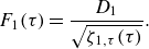 \begin{align} F_1(\tau )= \frac {D_1}{\sqrt {\zeta _{1,\tau }(\tau )}}. \end{align}
Similarly, $G_1(\tau )$
,
$G_1(\tau )$
, $F_2(\tau )$
, and
$F_2(\tau )$
, and $G_2(\tau )$
can be expressed as
$G_2(\tau )$
can be expressed as
 \begin{align} G_1(\tau )= \frac {D_2}{\sqrt {\zeta _{1,\tau }(\tau )}}, \quad F_2(\tau )= \frac {D_3}{\sqrt {\zeta _{2,\tau }(\tau )}} \quad \mbox{and} \quad G_2(\tau )= \frac {D_4}{\sqrt {\zeta _{2,\tau }(\tau )}}, \end{align}
where
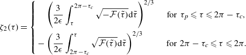 \begin{align} \zeta _2(\tau ) =\left \{ \begin{aligned} &\left (\frac {3}{2\epsilon } \int _\tau ^{2\pi -\tau _c} \sqrt {-\mathcal{F}(\tilde {\tau })} \mathrm{d}\tilde {\tau } \right )^{2/3} \quad\kern2pt \text{for} \;\, \tau _p\leqslant \tau \leqslant 2\pi -\tau _c,\\ - & \left (\frac {3}{2\epsilon } \int _{2\pi -\tau _c}^{\tau } \sqrt {\mathcal{F}(\tilde {\tau })} \mathrm{d}\tilde {\tau } \right )^{2/3} \quad \hspace {4mm} \;\;\text{for} \;\, 2\pi -\tau _c \leqslant \tau \leqslant 2\pi . \end{aligned} \right . \end{align}
The arbitrary constants $D_{1},\,D_2,\,D_3$
and
$D_{1},\,D_2,\,D_3$
and $D_4$
will be determined by using the initial conditions (3.3) and the continuity of
$D_4$
will be determined by using the initial conditions (3.3) and the continuity of $\eta (\tau )$
and
$\eta (\tau )$
and $\eta _{,\tau }(\tau )$
at
$\eta _{,\tau }(\tau )$
at $\tau _p=\pi$
. The initial conditions (3.3) give
$\tau _p=\pi$
. The initial conditions (3.3) give
 \begin{align} \begin{bmatrix} D_1 \\[6pt] D_2 \end{bmatrix} = \pi \sqrt {\zeta _{,\tau }(0)} \begin{bmatrix} Bi_{,\tau }\left (\zeta _1(0)\right ) \\[6pt] - Ai_{,\tau }\left (\zeta _1(0)\right ) \end{bmatrix} - \frac {\pi }{\sqrt {\zeta _{,\tau }(0)}} \left ( \frac {\mathrm{i}}{\epsilon }+ \frac {\zeta _{,\tau \tau }(0)}{2\zeta _{,\tau }(0)} \right ) \begin{bmatrix} Bi\left (\zeta _1(0)\right ) \\[6pt] - Ai\left (\zeta _1(0)\right ) \end{bmatrix}. \end{align}
The continuity of $\eta (\tau )$
and
$\eta (\tau )$
and $\eta _{,\tau }(\tau )$
at
$\eta _{,\tau }(\tau )$
at $\tau _p=\pi$
yields the following system of linear equations with unknowns
$\tau _p=\pi$
yields the following system of linear equations with unknowns $D_3$
and
$D_3$
and $D_4$
:
$D_4$
:
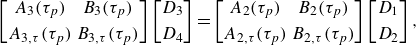 \begin{align} \begin{bmatrix} A_3(\tau _p) & B_3(\tau _p)\\[4pt] A_{3,\tau }(\tau _p) & B_{3,\tau }(\tau _p) \end{bmatrix} \begin{bmatrix} D_3 \\[4pt]D_4 \end{bmatrix} = \begin{bmatrix} A_2(\tau _p) & B_2(\tau _p)\\[4pt] A_{2,\tau }(\tau _p) & B_{2,\tau }(\tau _p) \end{bmatrix} \begin{bmatrix} D_1 \\[4pt] D_2 \end{bmatrix}, \end{align}
where
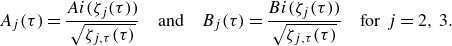 \begin{align} A_{j}(\tau )= \frac {Ai(\zeta _j(\tau ))}{\sqrt {\zeta _{j,\tau }(\tau )}} \quad \mbox{and} \quad B_{j}(\tau )= \frac {Bi(\zeta _j(\tau ))}{\sqrt {\zeta _{j,\tau }(\tau )}} \quad \mbox{for} \;\, j=2,\,3. \end{align}
Finally, the MAF solution of (2.21) over one period (and thus capturing both first and second turning points) is given by
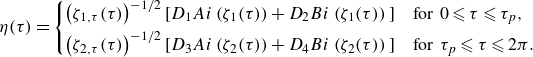 \begin{align} \eta (\tau )=\left \{\!\! \begin{aligned} & \left (\zeta _{1,\tau }(\tau )\right )^{-1/2} \big [D_1 Ai\left (\zeta _1(\tau )\right ) + D_2 Bi\left (\zeta _1(\tau )\right ) \big ] \quad \mbox{for} \;\, 0\leqslant \tau \leqslant \tau _p, \\ &\left (\zeta _{2,\tau }(\tau )\right )^{-1/2}\big [D_3 Ai\left (\zeta _2(\tau )\right ) + D_4 Bi\left (\zeta _2(\tau )\right )\big ]\quad \mbox{for} \;\, \tau _p \leqslant \tau \leqslant 2\pi . \end{aligned} \right . \end{align}
Comparison between numerical solution (blue) and MAF (dashed red) for one period for the case $\beta =0.5$
. The first and second turning points are, respectively,
$\beta =0.5$
. The first and second turning points are, respectively, $\tau _c$
and
$\tau _c$
and $2\pi -\tau _c$
; the unstable region predicted from (2.23) is shaded in grey.
$2\pi -\tau _c$
; the unstable region predicted from (2.23) is shaded in grey.
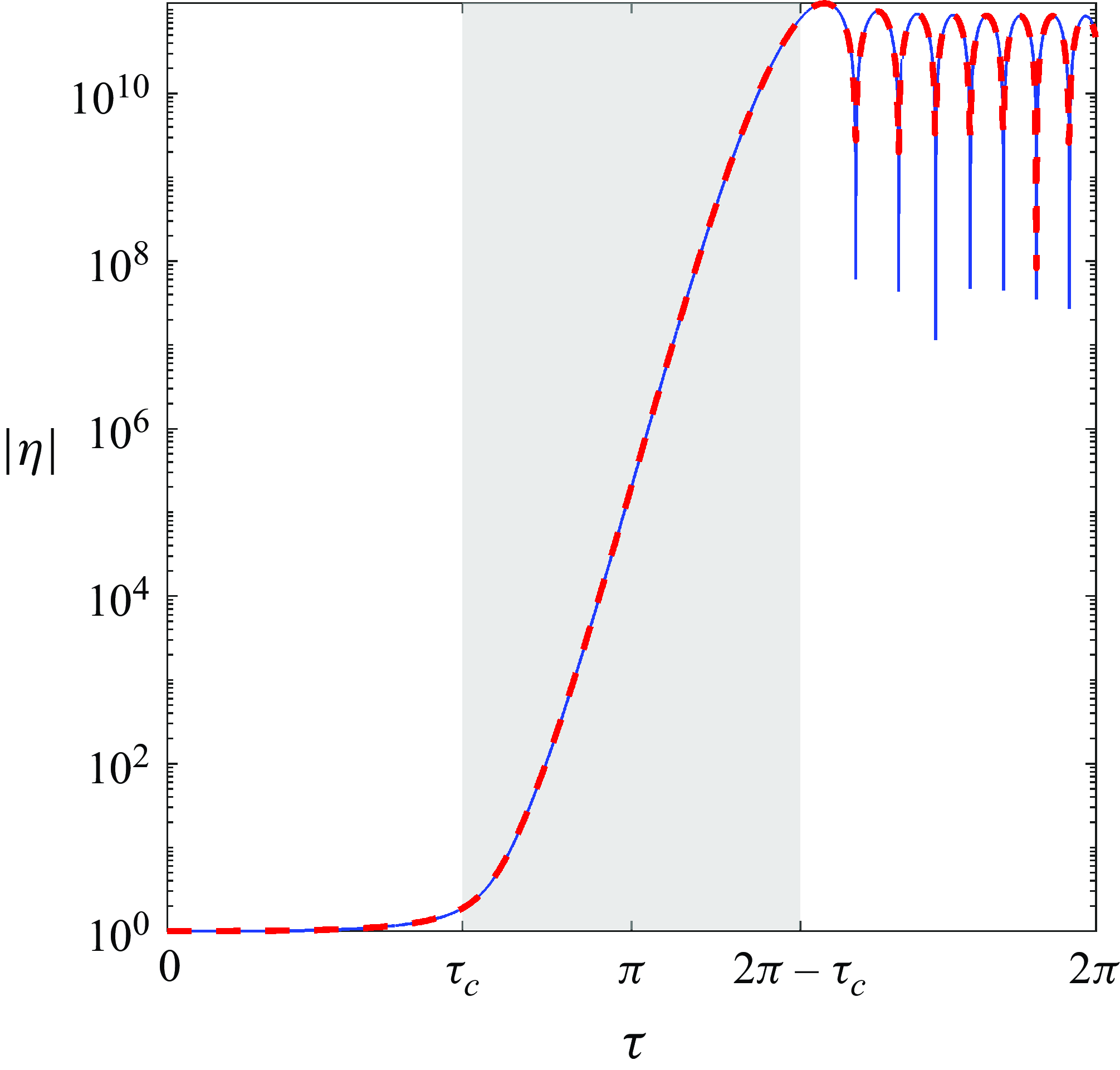
Figure 4, which is for the case $\beta \,{=}\,0.5$
, reveals that the MAF solution is nearly indistinguishable from the numerical solution. Unlike figure 3(c), figure 4 has been plotted for the entire
$\beta \,{=}\,0.5$
, reveals that the MAF solution is nearly indistinguishable from the numerical solution. Unlike figure 3(c), figure 4 has been plotted for the entire $2\pi$
period and thus includes the behaviour around both turning points. While figure 4 reveals oscillations after the second turning point, the existence of such a behaviour is contentious in reality since, even before the second turning point is reached, the flow is likely to enter the fully nonlinear stages of KH instability, making the linear solution invalid.
$2\pi$
period and thus includes the behaviour around both turning points. While figure 4 reveals oscillations after the second turning point, the existence of such a behaviour is contentious in reality since, even before the second turning point is reached, the flow is likely to enter the fully nonlinear stages of KH instability, making the linear solution invalid.
4. Numerical simulation: unsteady vortex blob method
Here, we extend the linear interfacial dynamics to the fully nonlinear stages via the vortex blob method, which is a standard numerical technique for capturing the nonlinear evolution of vortex sheets (Baker, Meiron & Orszag Reference Baker, Meiron and Orszag1982; Sohn, Yoon & Hwang Reference Sohn, Yoon and Hwang2010; Pozrikidis Reference Pozrikidis2011; Bhardwaj & Guha Reference Bhardwaj and Guha2018). The applicability of the vortex blob method to our two-layered oscillating flow problem is fully justified since the two-fluid interface is a vortex sheet, i.e. the tangential component of fluid velocity has a jump discontinuity. In vortex methods, the interface is described as a parametric curve $\boldsymbol{x}(s,t)=(x(s,t),z(s,t))$
with
$\boldsymbol{x}(s,t)=(x(s,t),z(s,t))$
with $s$
being the arc-length parameter, and evolves according to
$s$
being the arc-length parameter, and evolves according to
 \begin{equation} \boldsymbol{x}_{\!,t}=\boldsymbol{q}, \end{equation}
where $\boldsymbol{q}\,=\,({\overline {u}},\,{\overline {w}})\,=\,(\boldsymbol{u_1}+\boldsymbol{u_2})/2$
is the arithmetic mean of the velocities above (i.e.
$\boldsymbol{q}\,=\,({\overline {u}},\,{\overline {w}})\,=\,(\boldsymbol{u_1}+\boldsymbol{u_2})/2$
is the arithmetic mean of the velocities above (i.e. $\boldsymbol{u_1}\,{=}\,(u_1,\,w_1$
)) and below (i.e.
$\boldsymbol{u_1}\,{=}\,(u_1,\,w_1$
)) and below (i.e. $\boldsymbol{u_2}\,{=}\,(u_2,\,w_2$
)) the interface. For a domain that is periodic in the along-channel direction
$\boldsymbol{u_2}\,{=}\,(u_2,\,w_2$
)) the interface. For a domain that is periodic in the along-channel direction $x$
, the velocity
$x$
, the velocity $\boldsymbol{q}$
is obtained via the Birkhoff–Rott equation
$\boldsymbol{q}$
is obtained via the Birkhoff–Rott equation
 \begin{equation} \overline {u}-\mathrm{i} \overline {w} = \frac {\mathrm{i}}{2\lambda }\int _{0}^{\lambda }\widetilde {\gamma }\cot \left [\frac {\pi (\chi - \widetilde {\chi })}{\lambda }\right ] {\rm d}\widetilde {s}, \end{equation}
where $ \chi$
is the complex position of the interface:
$ \chi$
is the complex position of the interface: $ \chi = x(s,t) + \mathrm{i} z(s,t)$
,
$ \chi = x(s,t) + \mathrm{i} z(s,t)$
, $ \lambda$
is the wavelength and
$ \lambda$
is the wavelength and $\widetilde {\gamma }\,{=}\,\gamma (\widetilde {s},t)$
denotes the vortex-sheet strength, which is defined as the jump in the tangential velocities of the two fluids across the interface
$\widetilde {\gamma }\,{=}\,\gamma (\widetilde {s},t)$
denotes the vortex-sheet strength, which is defined as the jump in the tangential velocities of the two fluids across the interface
 \begin{equation} \gamma =(\boldsymbol{u_1}-\boldsymbol{u_2})\boldsymbol{\cdot} \hat {\boldsymbol{s}}. \end{equation}
In order to solve (4.2), the evolution equation for the vortex-sheet strength is needed. To obtain this, first we rewrite (2.2a )–(2.2b ) for each layer in a vectorial form
 \begin{equation} \frac {\mathrm{D}\boldsymbol {u_i}}{\mathrm{D}t} = -\frac {1}{\rho _0}\boldsymbol{\nabla} P_{i} - g\frac {\rho _{i}}{\rho _0}(\sin \alpha (t) \hat {\boldsymbol{x}} + \cos \alpha (t) \hat {\boldsymbol{z}} )+ 2 \alpha _{,t} \hat {\boldsymbol{y}} \times \boldsymbol{u_i}, \end{equation}
where $\boldsymbol{u_i}\,{=}\,(u_i,w_i)$
, and
$\boldsymbol{u_i}\,{=}\,(u_i,w_i)$
, and $i\,{=}\,1(2)$
implies upper (lower) layer. Subtracting the equation for
$i\,{=}\,1(2)$
implies upper (lower) layer. Subtracting the equation for $i\,{=}\,2$
from
$i\,{=}\,2$
from $i\,{=}\,1$
and projecting the resultant equation along the tangential direction (by taking an inner product with
$i\,{=}\,1$
and projecting the resultant equation along the tangential direction (by taking an inner product with $\boldsymbol{\hat {s}}$
) yields
$\boldsymbol{\hat {s}}$
) yields
 \begin{equation} \frac {{\rm D}\gamma }{{\rm D} t}+\gamma \frac {\partial \boldsymbol{q}}{\partial s}\,\boldsymbol{\cdot}\,\boldsymbol{\hat {s}}=g'(\sin \alpha (t) \hat {\boldsymbol{x}} + \cos \alpha (t) \hat {\boldsymbol{z}} ) \boldsymbol{\cdot\ \hat {s}}+[2 \alpha _{,t} \hat {\boldsymbol{y}} \times (\boldsymbol{u_1}-\boldsymbol{u_2})] \boldsymbol{\cdot\ \hat {s}}, \end{equation}
where ${\rm D}/{\rm D}t\,{=}\,\partial /\partial t + \boldsymbol{q \cdot \hat {s}}\, \partial /\partial s$
. In obtaining (4.5), the continuity of pressure across the interface has been used. Furthermore, using the identities
${\rm D}/{\rm D}t\,{=}\,\partial /\partial t + \boldsymbol{q \cdot \hat {s}}\, \partial /\partial s$
. In obtaining (4.5), the continuity of pressure across the interface has been used. Furthermore, using the identities $\hat {\boldsymbol{x}}\boldsymbol{\cdot} \hat {\boldsymbol{s}}=\partial x/\partial s$
and
$\hat {\boldsymbol{x}}\boldsymbol{\cdot} \hat {\boldsymbol{s}}=\partial x/\partial s$
and $\hat {\boldsymbol{z}}\boldsymbol{\cdot} \hat {\boldsymbol{s}}=\partial z/\partial s$
, we find that the last term on the right-hand side of (4.5), arising from the Coriolis acceleration, vanishes since the interface is a streamline
$\hat {\boldsymbol{z}}\boldsymbol{\cdot} \hat {\boldsymbol{s}}=\partial z/\partial s$
, we find that the last term on the right-hand side of (4.5), arising from the Coriolis acceleration, vanishes since the interface is a streamline
 \begin{align} (\hat {\boldsymbol{y}} \times \boldsymbol{u_{1,2}} ) \boldsymbol{\cdot} \hat {\boldsymbol{s}}=w_{1,2} \frac {\partial x}{\partial s}-u_{1,2}\frac {\partial z}{\partial s}=0. \end{align}
Previous studies with vortex methods have primarily been restricted to steady background flows (for example, see Sohn et al. (Reference Sohn, Yoon and Hwang2010) and references therein) although the method itself applies to unsteady flows. In our case, the explicit time dependence of the flow clearly manifests on the right-hand side of (4.5) through the angle of oscillation parameter $\alpha (t)$
.
$\alpha (t)$
.
For the numerical implementation, we first write (4.2) in a discretised fashion
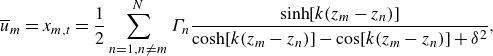 \begin{align}&\,\, \overline {u}_m = x_{m,t} = \frac {1}{2}\sum _{n=1, n \neq m}^{N} {\Gamma _{n}}\frac {\sinh [k(z_{m}-z_{n})]}{\cosh [k(z_{m}-z_{n})] - \cos [k(z_{m}-z_{n})] + \delta ^2}, \end{align}
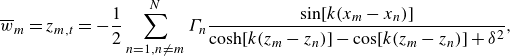 \begin{align}& \overline {w}_m= z_{m,t} = -\frac {1}{2}\sum _{n=1, n \neq m}^{N}{\Gamma _{n}}\frac {\sin [ k(x_{m}-x_{n})]}{\cosh [ k(z_{m}-z_{n})] - \cos [ k(z_{m}-z_{n})] + \delta ^2}, \end{align}
where $(\overline {u}_m,\overline {w}_m)$
is the velocity of the
$(\overline {u}_m,\overline {w}_m)$
is the velocity of the $m^{\mathrm{}}$
th point vortex (Lagrangian marker) at the location (
$m^{\mathrm{}}$
th point vortex (Lagrangian marker) at the location ( $x_m,z_m$
),
$x_m,z_m$
), $N$
denotes the total number of point vortices,
$N$
denotes the total number of point vortices, $k\,{=}\,2\pi /\lambda$
denotes the wavenumber and
$k\,{=}\,2\pi /\lambda$
denotes the wavenumber and $\delta$
denotes Kransy’s parameter (Krasny Reference Krasny1986) which regularises the otherwise singular kernel in (4.2). The parameter
$\delta$
denotes Kransy’s parameter (Krasny Reference Krasny1986) which regularises the otherwise singular kernel in (4.2). The parameter $\delta$
can be regarded as a proxy for viscous effects, numerically replacing point vortices with vortex ‘blobs’, and thereby adding a finite thickness to the otherwise discontinuous shear layer. Finally,
$\delta$
can be regarded as a proxy for viscous effects, numerically replacing point vortices with vortex ‘blobs’, and thereby adding a finite thickness to the otherwise discontinuous shear layer. Finally, $\Gamma _m$
denotes the circulation of the
$\Gamma _m$
denotes the circulation of the $m^{{}}$
th point vortex, which is given as follows:
$m^{{}}$
th point vortex, which is given as follows:
 \begin{equation} \Gamma _{m} = \gamma _{m} \Delta s_{m}, \end{equation}
where $ \Delta s_{m}$
is the arc length about the
$ \Delta s_{m}$
is the arc length about the $m^{{}}$
th point vortex
$m^{{}}$
th point vortex
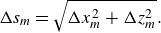 \begin{align} \Delta s_{m} = \sqrt { \Delta x_m^2 + \Delta z_m^2}. \end{align}
In the above equation, $\Delta x_m=(x_{m+1} - x_{m-1})/2$
and
$\Delta x_m=(x_{m+1} - x_{m-1})/2$
and $\Delta z_m=(z_{m+1} - z_{m-1})/2$
. Equations (4.7a
)–(4.7b
) succinctly show that the interaction between the point vortices representing the discretised vortex sheet leads to interface evolution.
$\Delta z_m=(z_{m+1} - z_{m-1})/2$
. Equations (4.7a
)–(4.7b
) succinctly show that the interaction between the point vortices representing the discretised vortex sheet leads to interface evolution.
Using (4.8) in (4.5), we obtain the discretised version of the circulation evolution equation
 \begin{equation} \Gamma _{m, t} = \Delta x_m \,g'\sin {\alpha (t)} + \Delta z_m\, g'\cos {\alpha (t)} . \end{equation}
Next, we numerically solve (4.7a
)–(4.7b
) along with (4.10) (where the definition of $\alpha (t)$
is given in (2.8)) using the fourth-order Runge–Kutta time integration scheme. To speed up the computation, we recast the governing equations into the slow-time variable
$\alpha (t)$
is given in (2.8)) using the fourth-order Runge–Kutta time integration scheme. To speed up the computation, we recast the governing equations into the slow-time variable $\tau$
. The system is initialised with a short, linear, interfacial gravity wave with the following interfacial displacement, written in a discretised fashion:
$\tau$
. The system is initialised with a short, linear, interfacial gravity wave with the following interfacial displacement, written in a discretised fashion: $z_m\,{=}\,a\cos (kx_m)$
, where
$z_m\,{=}\,a\cos (kx_m)$
, where $x_m\,{=}\,m/N$
,
$x_m\,{=}\,m/N$
, $k\,{=}\,2\pi$
and
$k\,{=}\,2\pi$
and $a\,{=}\,10^{-6}$
. The initial circulation of the
$a\,{=}\,10^{-6}$
. The initial circulation of the $m^{\mathrm{}}$
th point vortex is then given by
$m^{\mathrm{}}$
th point vortex is then given by
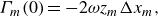 \begin{align} \Gamma _m(0)=-2\omega z_m \Delta x_m, \end{align}
where $\omega \!=\sqrt {g'k/2}\,{=}\,0.1772$
, and corresponds to
$\omega \!=\sqrt {g'k/2}\,{=}\,0.1772$
, and corresponds to $g'\,{=}\,0.01$
. Initially we take
$g'\,{=}\,0.01$
. Initially we take $N\,{=}\,400$
. With the progress of time, especially during the highly nonlinear stages, the interface can develop poor resolution in certain locations. To tackle this, we follow the vortex insertion scheme outlined in Sohn et al. (Reference Sohn, Yoon and Hwang2010). In this procedure, a threshold arc length
$N\,{=}\,400$
. With the progress of time, especially during the highly nonlinear stages, the interface can develop poor resolution in certain locations. To tackle this, we follow the vortex insertion scheme outlined in Sohn et al. (Reference Sohn, Yoon and Hwang2010). In this procedure, a threshold arc length $ \Delta s_{{thresh}}$
is defined; if the arc length at any location
$ \Delta s_{{thresh}}$
is defined; if the arc length at any location $ m$
becomes greater than the threshold, i.e.
$ m$
becomes greater than the threshold, i.e. $ \Delta s_{m}\,{\gt}\,\Delta s_{{thresh}}$
, then a point vortex is inserted. The
$ \Delta s_{m}\,{\gt}\,\Delta s_{{thresh}}$
, then a point vortex is inserted. The $x$
coordinate of the inserted vortex is taken to be the average of the
$x$
coordinate of the inserted vortex is taken to be the average of the $x$
coordinates of the
$x$
coordinates of the $m^{{}}$
th and
$m^{{}}$
th and $(m+1)^{{}}$
th vortices; the same approach is followed for the
$(m+1)^{{}}$
th vortices; the same approach is followed for the $z$
coordinate and the circulation. The Kransy parameter
$z$
coordinate and the circulation. The Kransy parameter $\delta$
is chosen accordingly to suppress spurious high wavenumber instabilities.
$\delta$
is chosen accordingly to suppress spurious high wavenumber instabilities.


Interface evolution for the case $\beta =0.8$
for
$\beta =0.8$
for $\tau =2.285, 2.315, 2.340$
and
$\tau =2.285, 2.315, 2.340$
and $2.395$
.
$2.395$
.
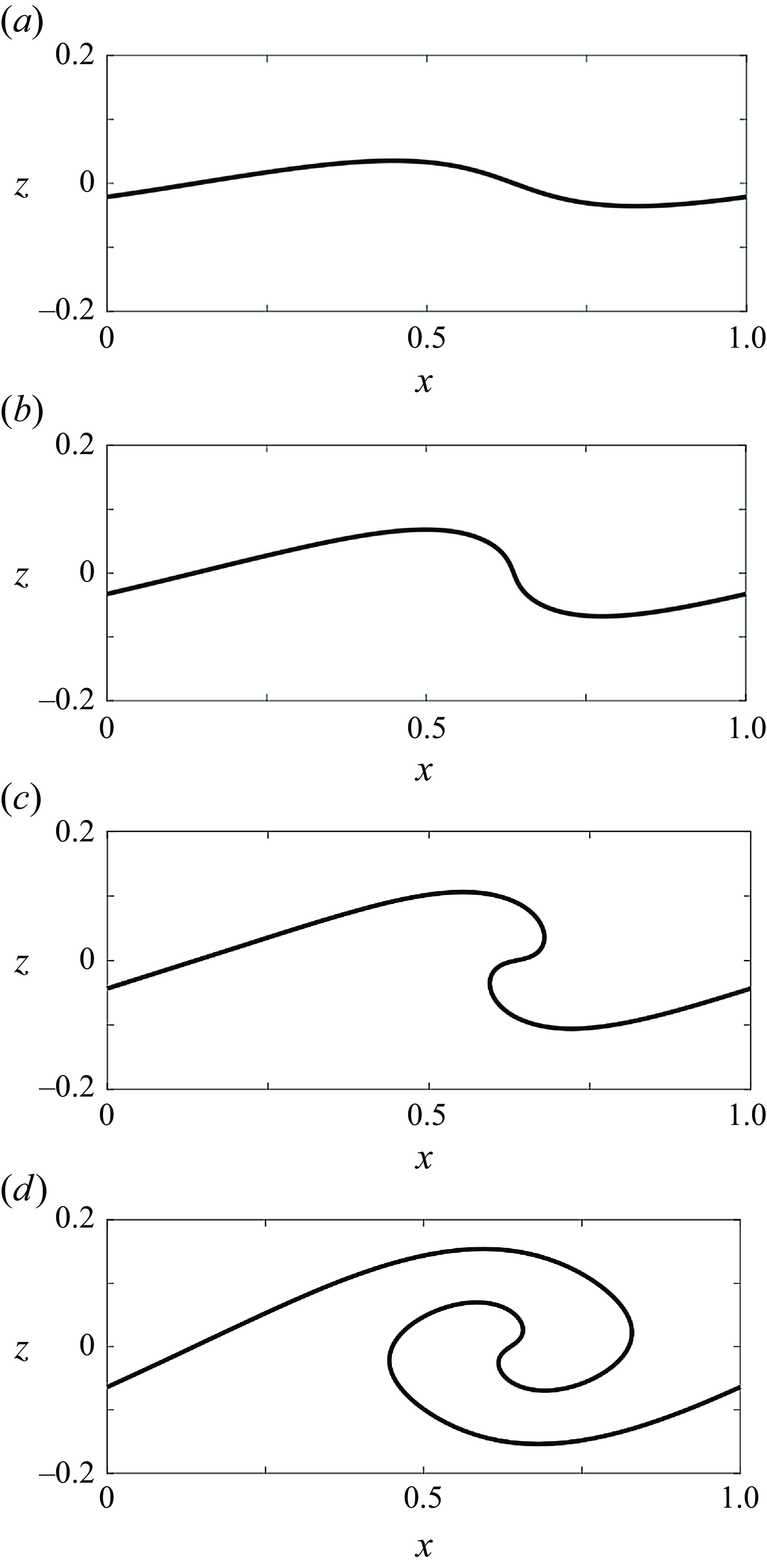
Figure 5 compares the interface evolution obtained from the linear equation (2.21) with the fully nonlinear solution obtained using the vortex blob method for two different $\beta$
values. The growth rate and the onset of instability predicted from the vortex method solution agree well with the linear theory.
$\beta$
values. The growth rate and the onset of instability predicted from the vortex method solution agree well with the linear theory.
Figure 6 shows the interface evolution for the case $\beta =0.8$
. The interface rolls up into a KH billow, qualitatively agreeing with the DNS results of Inoue & Smyth (Reference Inoue and Smyth2009) and Lewin & Caulfield (Reference Lewin and Caulfield2022). The numerical simulation is run until the billow saturates. Any further late-time dynamics may not be representative of the reality since the vortex method is strictly two-dimensional and hence does not capture the 3-D effects emanating from secondary instabilities, which can crucially alter the dynamical behaviour (Lewin & Caulfield Reference Lewin and Caulfield2022).
$\beta =0.8$
. The interface rolls up into a KH billow, qualitatively agreeing with the DNS results of Inoue & Smyth (Reference Inoue and Smyth2009) and Lewin & Caulfield (Reference Lewin and Caulfield2022). The numerical simulation is run until the billow saturates. Any further late-time dynamics may not be representative of the reality since the vortex method is strictly two-dimensional and hence does not capture the 3-D effects emanating from secondary instabilities, which can crucially alter the dynamical behaviour (Lewin & Caulfield Reference Lewin and Caulfield2022).
5. Physical interpretation and case studies
The oscillating tank system is a simplified model for studying instabilities arising in a temporally varying pycnocline in lakes, estuaries and oceans. Pycnocline oscillations are typically generated by wind forcing, or by diurnal and semi-diurnal tides interacting with underwater topography (Sanford et al. Reference Sanford, Sellner and Breitburg1990; Mihanović et al. Reference Mihanović, Orlić and Pasarić2009). During the summer months, many shelf seas and lakes reveal a two-layered density stratification (Lemmin et al. Reference Lemmin, Mortimer and Bäuerle2005; Mihanović et al. Reference Mihanović, Orlić and Pasarić2009; Guihou et al. Reference Guihou, Polton, Harle, Wakelin, O’Dea and Holt2018), providing ideal conditions to compare the flow field induced by low baroclinic mode oscillations of the pycnocline with the oscillating tank system. Below we provide two case studies, one for Lake Geneva and the other for the Chesapeake Bay.
5.1. Lake Geneva
We consider the background conditions of the summer of $1950$
given in Lemmin et al. (Reference Lemmin, Mortimer and Bäuerle2005):
$1950$
given in Lemmin et al. (Reference Lemmin, Mortimer and Bäuerle2005): $h_1\,{=}\,15$
m,
$h_1\,{=}\,15$
m, $h_2\,{=}\,175$
m,
$h_2\,{=}\,175$
m, $\rho _1\,{=}\,998.49\,\rm kg\,m^-{^3}$
(corresponding to
$\rho _1\,{=}\,998.49\,\rm kg\,m^-{^3}$
(corresponding to $19\,^\circ$
C) and
$19\,^\circ$
C) and $\rho _2\,{=}\,1000\,\rm kg\, m^-{^3}$
(corresponding to
$\rho _2\,{=}\,1000\,\rm kg\, m^-{^3}$
(corresponding to $5.5\,^\circ$
C). The frequency of mode-1 is
$5.5\,^\circ$
C). The frequency of mode-1 is $\omega _f\,{=}\,2.14\,{\times}$ $10^{-5}$
s
$10^{-5}$
s $^{-1}$
(period of
$^{-1}$
(period of $81.5$
h) and corresponds to a Kelvin seiche. The maximum width of the lake is
$81.5$
h) and corresponds to a Kelvin seiche. The maximum width of the lake is $13.8$
km and the maximum difference in thermocline excursions at the two extremities of the lake width (station-3 and station-8) due to mode-1 is
$13.8$
km and the maximum difference in thermocline excursions at the two extremities of the lake width (station-3 and station-8) due to mode-1 is $\approx \!2$
m. Hence,
$\approx \!2$
m. Hence, $\tan \alpha _f \approx \alpha _f = 2/13800=0.000145$
. Since the two layers are of unequal depths, the analysis provided in Appendix A will be applicable. The problem can be simplified since the lower layer is much deeper than the upper layer, which leads to the instability condition
$\tan \alpha _f \approx \alpha _f = 2/13800=0.000145$
. Since the two layers are of unequal depths, the analysis provided in Appendix A will be applicable. The problem can be simplified since the lower layer is much deeper than the upper layer, which leads to the instability condition $\beta \,{\gt}\,1/8$
; see (2.24). This yields
$\beta \,{\gt}\,1/8$
; see (2.24). This yields
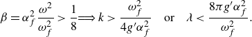 \begin{align} \beta =\alpha _f^2\frac { \omega ^2}{\omega _f^2}\gt \frac {1}{8} \implies k \gt \frac {\omega _f^2}{4g'\alpha _f^2}\,\,\,\,\, \mathrm{or}\,\,\,\,\, \lambda \lt \frac {8\pi g'\alpha _f^2}{\omega _f^2}. \end{align}
For the parameters of Lake Geneva, the above equation would imply that interfacial waves at the pycnocline shorter than $\lambda _{{long\hbox{-}wave\hbox{-}cut\hbox{-}off}}=17.03$
m will be rendered unstable. An interfacial wave of wavelength
$\lambda _{{long\hbox{-}wave\hbox{-}cut\hbox{-}off}}=17.03$
m will be rendered unstable. An interfacial wave of wavelength $17$
m will start to grow after
$17$
m will start to grow after $\tau _c=\cos ^{-1}[1-(2\beta )^{-1/2}] = 40$
hours (see Appendix A) from initiation of the mode-1 oscillation.
$\tau _c=\cos ^{-1}[1-(2\beta )^{-1/2}] = 40$
hours (see Appendix A) from initiation of the mode-1 oscillation.
5.2. Chesapeake Bay
Here, we consider the background conditions of May/June $1993$
of the Chesapeake Bay given in Frizzell-Makowski (Reference Frizzell-Makowski1997). In this case,
$1993$
of the Chesapeake Bay given in Frizzell-Makowski (Reference Frizzell-Makowski1997). In this case, $h_1\,{=}\,10$
m,
$h_1\,{=}\,10$
m, $h_2\,{=}\,13$
m,
$h_2\,{=}\,13$
m, $\rho _1\,{=}\,1004\,\rm kg\,m^-{^3}$
and
$\rho _1\,{=}\,1004\,\rm kg\,m^-{^3}$
and $\rho _2\,{=}\,1011\,\rm kg\,m^-{^3}$
. Pycnocline oscillations had a period of
$\rho _2\,{=}\,1011\,\rm kg\,m^-{^3}$
. Pycnocline oscillations had a period of $12$
h (
$12$
h ( $\omega _f\,{=}\,0.00014$
s
$\omega _f\,{=}\,0.00014$
s $^{-1}$
), which was generated by the interaction of semi-diurnal tides with a discontinuity in the bathymetry. Approximately
$^{-1}$
), which was generated by the interaction of semi-diurnal tides with a discontinuity in the bathymetry. Approximately $4$
m of vertical displacement over half of the wavelength (
$4$
m of vertical displacement over half of the wavelength ( $0.5\times 25$
km
$0.5\times 25$
km $=12.5$
km) of the internal tide was observed, yielding
$=12.5$
km) of the internal tide was observed, yielding $\tan \alpha _f \approx \alpha _f = 4/12500=0.00032$
. The two layers have unequal depths with
$\tan \alpha _f \approx \alpha _f = 4/12500=0.00032$
. The two layers have unequal depths with $r\,{=}\,h_1/h\,{=}\,0.435$
, yielding the instability condition
$r\,{=}\,h_1/h\,{=}\,0.435$
, yielding the instability condition $\beta \,{\gt}\,0.246$
. Following the analysis in Appendix A, we obtain
$\beta \,{\gt}\,0.246$
. Following the analysis in Appendix A, we obtain
 \begin{align} \beta =\alpha _f^2\frac { \omega ^2}{\omega _f^2}\gt 0.246 \implies k \gt \frac {0.492 \omega _f^2}{g'\alpha _f^2}\,\,\,\,\, \mathrm{or}\,\,\,\,\, \lambda \lt \frac {4.065\pi g'\alpha _f^2}{\omega _f^2}. \end{align}
Hence, for the parameters of Chesapeake Bay, interfacial waves at the pycnocline shorter than $\lambda _{{long\hbox{-}wave\hbox{-}cut\hbox{-}off}}=4.2$
m will become unstable. This implies that an interfacial wave of wavelength
$\lambda _{{long\hbox{-}wave\hbox{-}cut\hbox{-}off}}=4.2$
m will become unstable. This implies that an interfacial wave of wavelength $4$
m would start to grow
$4$
m would start to grow $\tau _c=5.4$
h (see (A6)) after the inception of the internal tide. However, it is important to note that these values should be taken as a rough estimate since the value of
$\tau _c=5.4$
h (see (A6)) after the inception of the internal tide. However, it is important to note that these values should be taken as a rough estimate since the value of $4.2$
m for the longest unstable wavelength is not large enough to disregard the finite-thickness effects of the pycnocline (pycnocline always has a finite thickness, however small).
$4.2$
m for the longest unstable wavelength is not large enough to disregard the finite-thickness effects of the pycnocline (pycnocline always has a finite thickness, however small).
6. Summary and conclusion
This study uses mathematical and numerical techniques to investigate the generation mechanism and fundamental characteristics of instabilities arising at the density interface in a two-layered oscillating channel flow. The set-up provides a simplified model for studying shear instabilities arising at the density interface due to the time-periodic shear generated by the slow oscillations of the density interface itself. This self-induced shear of the oscillating pycnocline may provide an alternate pathway to turbulence and diapycnal mixing in addition to that obtained via wind-induced shear in the upper ocean or the lake epilimnion.
The equation governing the density interface dynamics, given by (2.21), is a Schrödinger-type equation with a time-periodic potential. The small parameter $\epsilon$
, which is the ratio of the low-frequency pycnocline oscillations (forcing frequency) and the high-frequency short waves (that could be rendered unstable), encapsulates the separation of time scales. This makes (2.21) fundamentally different from the commonly studied time-periodic dynamical systems governed by Mathieu-type equations, which can lead to parametric instabilities. An inverse-Richardson-number-like non-dimensional parameter
$\epsilon$
, which is the ratio of the low-frequency pycnocline oscillations (forcing frequency) and the high-frequency short waves (that could be rendered unstable), encapsulates the separation of time scales. This makes (2.21) fundamentally different from the commonly studied time-periodic dynamical systems governed by Mathieu-type equations, which can lead to parametric instabilities. An inverse-Richardson-number-like non-dimensional parameter $\beta$
determines the necessary and sufficient stability condition of (2.21); for two layers of equal thickness, the flow becomes linearly unstable when
$\beta$
determines the necessary and sufficient stability condition of (2.21); for two layers of equal thickness, the flow becomes linearly unstable when $\beta \,{\gt}\,1/4$
. When the layers have unequal thickness, the stability condition depends on the ratio of layer thicknesses, see Appendix A. Once the instability condition is satisfied, the solution does not start to grow after
$\beta \,{\gt}\,1/4$
. When the layers have unequal thickness, the stability condition depends on the ratio of layer thicknesses, see Appendix A. Once the instability condition is satisfied, the solution does not start to grow after $\tau \,{=}\,0+$
, but rather tunnels into the unstable state after
$\tau \,{=}\,0+$
, but rather tunnels into the unstable state after $\tau \,{=}\,\tau _c$
. Using the parameters of a DNS case study in Lewin & Caulfield (Reference Lewin and Caulfield2022), we show that our theory correctly predicts the time of onset of instability. Next, we study the interface evolution by numerically solving (2.21) and compare it with the asymptotic solution obtained via the MAF method. We show that MAF provides a uniformly valid composite solution over the entire period (which includes two turning points) and reveals an excellent agreement with the numerical solution. To evaluate the temporal growth rate, we compute the Floquet exponents; furthermore, we also derive the exact normal-mode growth rate obtained for various steady-state-based approximations of the background flow. We observe that the normal-mode theory implemented on a background flow that considers the maximum velocity in each layer (as opposed to the time average over a period) provides a highly accurate growth rate prediction. The normal-mode growth rate is shown to exactly match the classical vortex-sheet KH instability, thereby conclusively proving that the instability is of KH type. Next, we extend the linear analysis of the interface evolution to the fully nonlinear stages via the unsteady vortex blob method. While the standard vortex blob method is commonly implemented for steady background flows, the procedure also applies to time-dependent flows. This needs modification to the circulation evolution equation typically used in vortex methods problems with density stratification. We derive the unsteady circulation evolution (4.10), which captures the explicit time dependence of the flow. The time of the onset of instability as well as the growth rate show good agreement with the predictions from the linear analysis. During the nonlinear stages, the interface rolls up into KH billows, agreeing with the previous DNS studies (Inoue & Smyth Reference Inoue and Smyth2009; Lewin & Caulfield Reference Lewin and Caulfield2022).
$\tau \,{=}\,\tau _c$
. Using the parameters of a DNS case study in Lewin & Caulfield (Reference Lewin and Caulfield2022), we show that our theory correctly predicts the time of onset of instability. Next, we study the interface evolution by numerically solving (2.21) and compare it with the asymptotic solution obtained via the MAF method. We show that MAF provides a uniformly valid composite solution over the entire period (which includes two turning points) and reveals an excellent agreement with the numerical solution. To evaluate the temporal growth rate, we compute the Floquet exponents; furthermore, we also derive the exact normal-mode growth rate obtained for various steady-state-based approximations of the background flow. We observe that the normal-mode theory implemented on a background flow that considers the maximum velocity in each layer (as opposed to the time average over a period) provides a highly accurate growth rate prediction. The normal-mode growth rate is shown to exactly match the classical vortex-sheet KH instability, thereby conclusively proving that the instability is of KH type. Next, we extend the linear analysis of the interface evolution to the fully nonlinear stages via the unsteady vortex blob method. While the standard vortex blob method is commonly implemented for steady background flows, the procedure also applies to time-dependent flows. This needs modification to the circulation evolution equation typically used in vortex methods problems with density stratification. We derive the unsteady circulation evolution (4.10), which captures the explicit time dependence of the flow. The time of the onset of instability as well as the growth rate show good agreement with the predictions from the linear analysis. During the nonlinear stages, the interface rolls up into KH billows, agreeing with the previous DNS studies (Inoue & Smyth Reference Inoue and Smyth2009; Lewin & Caulfield Reference Lewin and Caulfield2022).
Finally, we provide a physical context to the two-layered oscillating tank model by considering two case studies – Lake Geneva and Chesapeake Bay. Each of these sites reveals pycnocline oscillations, and using the available data, we obtain the stability condition, estimate the time of onset of the shear instabilities as well as the long-wavelength cutoff.
As a closing remark, we reiterate the fact that stability analysis with discontinuous profiles provides spurious growth rates (ultraviolet catastrophe), which necessitates stability analysis of background flows with finite shear layer thickness. The latter is also essential for obtaining the wavenumber corresponding to the maximum growth rate, as well as a short-wavelength cutoff, which cannot be obtained from discontinuous analysis. Despite these limitations, the two-layered configuration studied in this paper provides a foundational basis for the unsteady shear instability mechanism, makes the problem analytically (or semi-analytically) tractable through a simple governing equation, and also provides the necessary and sufficient condition for instability, which leads to key predictions (e.g. the time of onset of instability) that excellently compare with numerical results obtained from smooth profiles.
Acknowledgements.
We sincerely thank Dr S. Lewin from the University of California, Berkeley, and the two anonymous reviewers for the helpful comments and suggestions. We are grateful to Dr S. Lewin for running the DNS, which allowed us to compare the $\tau _c$
value from our predictions with the DNS results. We also thank the Associate Editor, Professor N. Balmforth, from the University of British Columbia, for his insightful comments. A.G. thanks Dr J. Polton from the National Oceanographic Centre, Liverpool for fruitful discussions on oceanographic applications of the problem.
$\tau _c$
value from our predictions with the DNS results. We also thank the Associate Editor, Professor N. Balmforth, from the University of British Columbia, for his insightful comments. A.G. thanks Dr J. Polton from the National Oceanographic Centre, Liverpool for fruitful discussions on oceanographic applications of the problem.
Declaration of interests.
The authors report no conflict of interest.
Appendix A. Derivation of the stability condition for two layers of unequal depths
Let us consider the two layers having different depths, denoted by $h_1$
and
$h_1$
and $h_2$
. The background state density distribution is then given by
$h_2$
. The background state density distribution is then given by
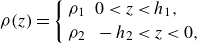 \begin{align} \rho (z) = \left \{ \begin{aligned} & \rho _1\,\,\, 0\lt z\lt h_1, \\ & \rho _2\,\,\, -h_2\lt z\lt 0, \end{aligned} \right . \end{align}
where $h_2\,{=}\,h-h_1$
, in which
$h_2\,{=}\,h-h_1$
, in which $h$
represents the total channel depth. Following the method outlined in § 2.1, the background state velocity profile is given by
$h$
represents the total channel depth. Following the method outlined in § 2.1, the background state velocity profile is given by
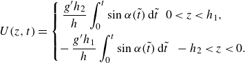 \begin{align} U(z,t)=\left \{\!\! \begin{aligned} & \,\,\frac {g' h_2}{h} \int _0^t\sin \alpha (\tilde {t})\, \mathrm{d}\tilde {t} \,\,\, 0\lt z\lt h_1 ,\\ &-\frac {g' h_1}{h} \int _0^t\sin \alpha (\tilde {t})\, \mathrm{d}\tilde {t}\,\,\, -h_2\lt z\lt 0. \end{aligned} \right . \end{align}
Under the assumption of small oscillations, the background state velocity profile simplifies to
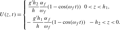 \begin{align} U(z,t)=\left \{\!\! \begin{aligned} & \,\,\frac {g' h_2}{h}\frac {\alpha _f}{\omega _f} (1-\cos (\omega _f t ))\,\,\, 0\lt z\lt h_1 ,\\ &-\frac {g' h_1}{h} \frac {\alpha _f}{\omega _f} (1-\cos (\omega _f t))\,\,\, -h_2\lt z\lt 0. \end{aligned} \right . \end{align}
Following the procedure in § 2.2, infinitesimal perturbations are added to the background state. The waves are assumed to be significantly shorter than the depth of the individual layers, i.e. $kh_1\,{\gg}\,1$
and
$kh_1\,{\gg}\,1$
and $kh_2\,{\gg}\,1$
. The evolution equation of the interface
$kh_2\,{\gg}\,1$
. The evolution equation of the interface $\eta (\tau )$
between the two fluid layers under the Boussinesq approximation is given by
$\eta (\tau )$
between the two fluid layers under the Boussinesq approximation is given by
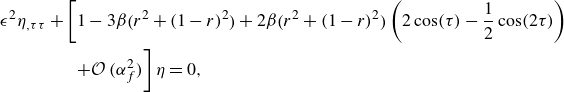 \begin{align} &\epsilon ^2\eta _{,\tau \tau } + \left [ 1 - 3\beta \big(r^2+(1-r)^2\big) + 2\beta \big(r^2+(1-r)^2\big) \left ( 2\cos (\tau ) -\frac {1}{2}\cos (2\tau )\right ) \right .\nonumber \\ &\qquad\qquad \left . + \vphantom{\frac {1}{2}}\mathcal{O}\,\big(\alpha _f^2\big)\right ] \eta =0, \end{align}
where $r\,{=}\,h_1/h$
. All variables and parameters are the same as in § 2.2. The necessary and sufficient condition for instability is found to be
$r\,{=}\,h_1/h$
. All variables and parameters are the same as in § 2.2. The necessary and sufficient condition for instability is found to be
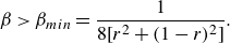 \begin{align} \beta \gt \beta _{{min}}= \frac {1}{8\big[r^2+(1-r)^2\big]}. \end{align}
Since $r\in (0,1)$
, this implies that
$r\in (0,1)$
, this implies that $1/8\lt \beta _{{min}} \leqslant 1/4$
.
$1/8\lt \beta _{{min}} \leqslant 1/4$
.
The turning point $\tau _c$
, marking the time at which the flow tunnels into the unstable region is given by
$\tau _c$
, marking the time at which the flow tunnels into the unstable region is given by
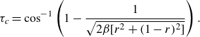 \begin{equation} \tau _c=\cos ^{-1} \left ( 1-\frac {1}{\sqrt {2\beta \big[r^2+(1-r)^2\big ]}}\right). \end{equation}
The maximum growth rate obtained from the normal-mode analysis is as follows:
 \begin{equation} \sigma _{{normal\hbox{-}mode}}=\frac {\sqrt {8\beta \big[r^2+(1-r)^2\big]- 1}}{\epsilon }. \end{equation}
In a typical oceanographic scenario, the depth of the pycnocline is much smaller than the total depth of the ocean, i.e. $r\,{\ll}\,1$
. In this situation, the instability condition becomes
$r\,{\ll}\,1$
. In this situation, the instability condition becomes $\beta \,{\gt}\,1/8$
, the instability will start after
$\beta \,{\gt}\,1/8$
, the instability will start after $\tau _c=\cos ^{-1}[1-(2\beta )^{-1/2}]$
, and the maximum growth rate obtained from the normal-mode method simplifies to
$\tau _c=\cos ^{-1}[1-(2\beta )^{-1/2}]$
, and the maximum growth rate obtained from the normal-mode method simplifies to $\sigma _{{normal\hbox{-}mode}}=\sqrt {8\beta -1}/\epsilon$
.
$\sigma _{{normal\hbox{-}mode}}=\sqrt {8\beta -1}/\epsilon$
.


 Open access