


Introduction
Debris flows are mass-wasting events induced by intense rainfall that can rapidly and destructively transport quantities of sediment, large rocks, and trees down a slope, following and reorganizing existing stream channels (e.g., Coussot and Meunier, Reference Coussot and Meunier1996; Iverson, Reference Iverson1997). Debris-flow events represent substantial geohazards that can transport enough sediment to damage or destroy infrastructure, fundamentally altering landscape substrate in addition to threatening lives and property. Debris flows intersecting with the built environment are one of the most common types of geologic hazard affecting society (Fidan et al., Reference Fidan, Tanyaş, Akbaş, Lombardo, Petley and Görüm2024). Wildfire contributes to debris-flow occurrence through the removal of vegetation that formerly intercepted rainfall and stabilized slopes. Wildfire further affects slope stability with intense heat, thermally altering soils that produce hydrophobic conditions conducive to overland flow rather than infiltration of rainfall. The role of fire with debris flows is becoming better understood through systematic studies that focus on sediment movement post-wildfire (Cannon and Gartner, Reference Cannon and Gartner2005; Shakesby and Doerr, Reference Shakesby and Doerr2006; Santi et al., Reference Santi, deWolf, Higgins, Cannon and Gartner2008; Kean et al., Reference Kean, Staley and Cannon2011, Reference Kean, Staley, Lancaster, Rengers, Swanson, Coe, Hernandez, Sigman, Allstadt and Lindsay2019; Lancaster et al., Reference Lancaster, Swanson, Lukashov, Oakley, Lee, Spangler and Hernandez2021; McGuire et al., Reference McGuire, Ebel, Rengers, Vieira and Nyman2024; Santi and Rengers, Reference Santi and Rengers2020; Thomas et al., Reference Thomas, Kean, McCoy, Lindsay, Kostelnik, Cavagnaro and Rengers2023). Many debris flows occur without antecedent fire events, but wildfires can increase the probability, as well as the size and frequency of occurrence in a given watershed (Korup and Clague, Reference Korup and Clague2009; Staley et al., Reference Staley, Negri, Kean, Laber, Tillery and Youberg2017; Tang et al., Reference Tang, McGuire, Rengers, Kean, Staley and Smith2019a, Reference Tang, McGuire, Rengers, Kean, Staley and Smith2019b; refer to review by McGuire et al., Reference McGuire, Ebel, Rengers, Vieira and Nyman2024).
The conditions under which debris flows develop are intensifying in the western United States as climate warms, underscoring the need to better understand debris-flow hazards in steep, mountainous settings. Wildfires, whether caused by natural lightning ignition or by human activity or equipment, have increased in size and severity in western North America due to twentieth-century forest fire–suppression efforts, allowing vegetation to accumulate, and exacerbated seasonal drying of vegetation in a warmer climate, as many studies have shown (e.g., Abatzoglou and Williams, Reference Abatzoglou and Williams2016; Abatzoglou et al., Reference Abatzoglou, Williams and Barbero2019; Williams et al., Reference Williams, Abatzoglou, Gershunov, Guzman-Morales, Bishop, Balch and Lettenmaier2019; Prein et al., Reference Prein, Coen and Jaye2022; Cunningham et al., Reference Cunningham, Williamson and Bowman2024). The fire regime is expected to intensify further in the western United States (and particularly in California, where the large population and economy are at already elevated risk from fire hazards) under future, warmer conditions (Prein et al., Reference Prein, Coen and Jaye2022; Turco et al., Reference Turco, Abatzoglou, Herrera, Zhuang, Jerez, Lucas, AghaKouchak and Cvijanovic2023; U.S. Global Change Research Program, Reference Crimmins, Avery, Easterling, Kunkel, Stewart and Maycock2023). Simultaneously, increasing hydrologic volatility is subjecting California and much of the western United States to a greater likelihood of extreme rainfall during a sharper, albeit shorter, winter wet season (Swain et al., Reference Swain, Langenbrunner, Neelin and Hall2018, Reference Swain, Prein, Abatzoglou, Albano, Brunner, Diffenbaugh, Singh, Skinner and Touma2025; Huang et al., Reference Huang, Stevenson and Hall2020; Luković et al., Reference Luković, Chiang, Blagojević and Sekulić2021). Therefore, the risk from debris flows, especially those developing in recently burned watersheds, is growing (Kean and Staley, Reference Kean and Staley2021). Excess sediment from watersheds experiencing fire and intense rain can impede water quality and infrastructure function even where debris flows do not develop, requiring management and mitigation (Sankey et al., Reference Sankey, Kreitler, Hawbaker, McVay, Miller, Mueller, Vaillant, Lowe and Sankey2017; East and Sankey, Reference East and Sankey2020; Basso et al., Reference Basso, Mateus, Ramos and Vieira2021; Jong-Levinger et al., Reference Jong-Levinger, Banerjee, Houston and Sanders2022).
This study documents the timing and occurrence of several pre–European settlement debris flows in northern California. The studied debris flows, which were presumed to be Holocene to historical before this investigation, preserve within their facies information on the temporal pattern and possible causes for prehistoric activation of adjacent fluvial catchments on the north slope of a mountain known as Shasta Bally. This mountain is within Whiskeytown National Recreation Area (WHIS), is the most prominent landform within the park (Fig. 1), and comprises an exposed Jurassic age batholith. The mountain is part of the Trinity Range within the Klamath Mountains of northwestern California and is one of the numerous peaks comprising metamorphic and igneous lithologies, including weathered and decomposing granitoid facies. WHIS is situated within the heart of this range and features steep and rugged topography (Fig. 2). Shasta Bally flanks are composed principally of biotite-hornblende granodiorite and quartz diorite with some associated gneiss and amphibolite, including quartz diorite that is 40% hornblende and biotite (Albers et al., Reference Albers, Kinkel, Drake and Irwin1964). This bedrock composition is prone to weathering into clays and grus, a very coarse granular material that is susceptible to mobilization (Albers, Reference Albers1964). The eastern Klamath Mountains, including WHIS, have a Mediterranean climate with a wet season between October and May; the study area is on the boundary between classes Csa and Csb in the Köppen-Geiger climate classification system (Beck et al., Reference Beck, McVicar, Vergopolan, Berg, Lutsko, Dufour, Zeng, Jiang, van Dijk and Miralles2023).
General area map, that includes information on park infrastructure, of Whiskeytown National Recreation Area and inset is location (star) within North America. Dashed box is the outline for location of Figure. 2. Shasta Bally is the highest point in the park at 1893 m above sea level (asl); 6209 ft asl). Base map data are from Environmental Systems Research Institute, Inc. (ESRI).

Image developed from 1 m 3D Elevation Program (3DEP) LIDAR data from the U.S. Geological Survey. Locations mentioned in the text are (A) the beach area of Brandy Creek at the reservoir pool; (B) Sheep Camp area; (C) Whiskeytown Environmental School (WES) Camp location, Bluebird Meadow; and (D) the constriction for the “canyon” downstream of the WES Camp on Clear Creek.

Debris flows often initiate in colluvial hollows or gullied drainages, where accumulated sediment from previous erosion events is mobilized by excess runoff (Cannon and Gartner, Reference Cannon and Gartner2005). In WHIS, which has historically experienced debris flows, the most recent events were minor, albeit with some infrastructure impacts. Paradoxically, following the major 2018 Carr Fire, no clearly identifiable debris-flow activity occurred, despite 97% of the park having burned and intense rain occurring in the first winter post-fire (East et al., Reference East, Logan, Dartnell, Lieber-Kotz, Cavagnaro, McCoy and Lindsay2021). Yet, there is ample evidence for earlier and large debris-flow events (Fig. 3) in the area, especially in the Brandy Creek watershed, where boulder levees intertwine within popular picnic and hiking trails along the stream bank. Other drainages also show signs of past debris-flow events: boulder levees, bedrock scoured channels and debris fans, and terraces at stream junctures are common landforms. What is not well known are the chronology and frequency of occurrence of debris flows before European settlement.
Typical appearance of debris-flow levees (boulder-rich deposits) in the mid-watershed of Brandy Creek, with forest cover. Image is looking to the south-southwest located near the Sheep Camp area. These forms are evidence for larger debris-flow events that predate the park. Trees in the area had trunk bases upward of 1 m (3 ft) in diameter. NPS photo, courtesy of Jack Wood.

The modern landscape within the monument has been shaped mostly by climate change and ecological succession during the Holocene and the Pleistocene. Anthropogenic influences cannot be dismissed, however (Fry and Stephens, Reference Fry and Stephens2006). Incidental to the arrival of Euro-American settlement, fire suppression came with the mining, agricultural, and forest harvesting efforts. The geology of the Klamath Mountains does contain economic mineral deposits, and extractive efforts in the nineteenth and early twentieth centuries yielded some gold and copper through placer, hydraulic, and hard rock mining. Mine tailings could be sources for debris flows, and several productive mines occurred in the vicinity of the Shasta Bally, but most seem to be located near or within the confines of the modern reservoir. Within the Brandy Creek drainage, only minor works were attempted, with no deep workings and only shallow shafts or pockets developed (Toogood, Reference Toogood1978).
Debris flows have played a critical role in shaping this landscape, particularly in response to climate variability and vegetation changes. Elsewhere in western North America, evidence from prehistoric debris-flow deposits indicates that their frequency of occurrence is enhanced by periods of increased rainfall intensity and persistent drought that likely stressed stabilizing vegetation, especially following the transition out of the last glacial (Youberg et al., Reference Youberg, Webb, Fenton and Pearthree2014). Geochronological data indicate some especially large events occurred during the Pleistocene–Holocene transition, with subsequent smaller events occurring in response to later Holocene climatic shifts (Collins et al., Reference Collins, Reid, Coe, Kean, Baum, Jibson, Godt, Slaughter, Stock, Sassa, Mikoš, Sassa, Bobrowsky, Takara and Dang2021).
Historical debris flows, however, seem to be readily triggered by the combination of wildfires and intense storms; yet this is similar to the processes that have shaped the landscape for millennia. The timing of periods of instability that resulted in debris flows in and around WHIS could be elucidated from a better understanding of the sedimentary nature of the deposits and through the use of radiocarbon and optically stimulated luminescence (OSL) dating methods. Discerning the periods of debris-flow activity, amount and type of sediment moved, and locations on the landscape that are repeatedly affected by the debris flows could add understanding to future mitigation, development, and park property protection efforts.
Hillslopes commonly shed large quantities of sediment in the aftermath of wildfire, with potential hazards for downstream communities, infrastructure, and water supply. The size and duration of these effects vary widely and have not been measured in detail for many areas within the Klamath Mountains. The National Park Service (NPS), the U.S. Geological Survey (USGS), and other partners are collaborating to understand prehistoric debris-flow activity in WHIS. This effort is an additional avenue of investigation after recent studies of postfire landscape evolution, including after the 2018 Carr Fire, a federally declared major disaster (East et al., Reference East, Logan, Dartnell, Lieber-Kotz, Cavagnaro, McCoy and Lindsay2021). That earlier effort focused on evaluating geohazards that affect Whiskeytown Lake and surrounding watersheds. This study was designed to use geochronologic data to elucidate the timing of prehistoric debris-flow activity in WHIS, together with observations of sediment composition to determine whether the debris flows mobilized burned material. Understanding past debris-flow activity in this setting can inform assessments of potential future risks to water supply from the large, federally managed Whiskeytown Lake, a reservoir formed by the construction of Whiskeytown Dam in 1963 and used for regional agricultural water supply and storage for hydroelectric use. In addition to the geohazards implications of debris flows and floods, in a warming climate with a more intense fire regime and expected greater watershed sediment production (Sankey et al., Reference Sankey, Kreitler, Hawbaker, McVay, Miller, Mueller, Vaillant, Lowe and Sankey2017; Swain et al., Reference Swain, Langenbrunner, Neelin and Hall2018; East and Sankey, Reference East and Sankey2020; Gutierrez et al., Reference Gutierrez, Hantson, Langenbrunner, Chen, Jin and Randerson2021; MacDonald et al., Reference MacDonald, Wall, Enquist, LeRoy, Bradford, Breshears and Brown2023; Turco et al., Reference Turco, Abatzoglou, Herrera, Zhuang, Jerez, Lucas, AghaKouchak and Cvijanovic2023), prehistoric debris-flow frequency can be used to evaluate the susceptibility of downstream water resources to sedimentation and water-quality effects associated with major sediment-runoff events (Hallema et al., Reference Hallema, Robinne and Bladon2018; B.P. Murphy et al., Reference Murphy, Yocom and Belmont2018; Basso et al., Reference Basso, Mateus, Ramos and Vieira2021; Randle et al., Reference Randle, Morris, Tullos, Weirich, Kondolf, Moriasi, Annandale, Fripp, Minear and Wegner2021; Williams et al., Reference Williams, Livneh, McKinnon, Hansen, Mankin, Cook and Smerdon2022; Belongia et al., Reference Belongia, Wagner, Seipp and Ajami2023; S.F. Murphy et al., Reference Murphy, Alpers, Anderson, Banta, Blake, Carpenter and Clark2023; Dow et al., Reference Dow, East, Sankey, Warrick, Kostelnik, Lindsay and Kean2024).
Methods
Field trenching, natural exposure (terrace), and boulder “lifting”
We employed a sampling strategy to ensure representative sample collection across the wide range of Quaternary and historical sediment movement and preservation in the drainages of WHIS. Accessing and investigating the targeted sediments in this project were weighted with regard to the impacts from excavation disturbance on the rich cultural landscape that WHIS protects. Known archeological sites were avoided, and sampling plans were reviewed on-site with park cultural staff and representatives from tribal entities. Excavation options were limited along the Clear, Brandy, and Paige Boulder Creeks, due to the density of known cultural resources. However, suitable sites in the Brandy Creek watershed were accessible enough for a targeted and more systematic sampling approach without disturbing cultural sites. Brandy Creek initiates high (∼1830 m above sea level [asl]/6000 ft asl) on the Shasta Bally, is a tributary to Clear Creek (the main drainage impounded by Whiskeytown Dam), and exhibits numerous debris-flow characteristic levee deposits (Albers et al., Reference Albers, Kinkel, Drake and Irwin1964). The proximity of the two watersheds ensures (as much as possible), they have similar responses to fire- and precipitation-induced debris flows.
OSL dating on sediment collected from debris flows results in heterogenous bleaching of both quartz and potassium feldspar (Zhao et al., Reference Zhao, Jørkov Thomsen, Murray, Wei, Pan, Song, Zhou, Chen, Zhao and Chen2015), as these deposits commonly are emplaced rapidly and thus have very limited exposure to light before deposition. Care must be taken when using multi-grain aliquots, as grains that were variably and incompletely bleached before deposition can yield ages that are significantly older than the sample’s burial age. These sediments suffer from significant incomplete bleaching, so the main emphasis should be on single-grain OSL measurements. However, we only had access to multi-grain measurements, so we tried to selectively sample sediment from distal flows to increase the probability of completely reset single grains. In addition, we ensured that the majority of the quartz grains had a visually dominant fast luminescence component (Fig. 4), tested the thermal transfer during lab protocols, checked that dose-recovery experiments were undertaken, and evaluated the burial doses by applying various minimum age models to the measured dose distributions (Galbraith, Reference Galbraith1990; Galbraith and Roberts, Reference Galbraith and Roberts2012; Duller, Reference Duller2004; Zhao et al., Reference Zhao, Jørkov Thomsen, Murray, Wei, Pan, Song, Zhou, Chen, Zhao and Chen2015; Yongqiang et al., Reference Yongqiang, Yonggang and Mao2024).
Example of luminescence characteristics and analysis from software-generated measurement parameters of a typical quartz sediment beneath one of the sampled boulders, in this case USGS-3382. (A) Probability plot of all measured aliquots (n = 38). Blue line follows peaks generated by the measured Gray of each aliquot. The height of the blue line is higher when the number of aliquots with similar Gray values is grouped (known as population). The red hashed area between 3.5 to 4.0 Gy is the central age model (within 2-sigma). This probability plot shows three small populations and two large populations. The largest population shows a distinct bifurcation at the top in response errors associated with measurements. (B) Example of the circular scale radial plot of Galbraith et al. (Reference Galbraith1990) showing the minimum age model (MAM) as generated by RadialPlotter (Vermeesch, 2009). The minimum age and age dispersion are read from the intersection of the 2-sigma line to the curves scale to the right (which ranges from 13 to 1.2 Gy; the 2-sigma overlap is unusually tight and cannot be fully distinguished in the plot as it looks like one line). The slope of a line connecting the origin (x = 0, y = 0) of a radial plot with a data point or measurement value (xj, yj) equals zj, and the horizontal distance along the x-axis is a measure of its precision (more precise errors are closest to the curved axis). Thus, the radial plot simultaneously visualizes a measurement’s value and precision (Vermeesch, 2009). The data are color coded between green (0.10) or lower values of Gray and red (1.0) or higher values of Gray. It is assumed that higher values of Gray may be caused by inherited luminescence that was not fully zeroed at the latest transport. (C) Example of the decay curves for aliquot 25 for the fast component of quartz optically stimulated luminescence (OSL). These curves include the natural as well as regenerated OSL from exposure to a beta source. Time is measured in seconds and OSL (counts per 0.15 seconds). The OSL signal is integrated over the initial part of the decay and refers to the number of photons given off when stimulated with a continuous-wave LED-generated blue wavelength. The largest number of photon counts is measured within the first second of LED stimulation. This phenomenon is highlighted within the twin red lines near the 0 second time on the left as a peak near 4000. Background counts for subtraction to the measured counts are taken between the twin green lines of light levels (photons) measured at the end of the stimulation at about 200 OSL counts. (D) Example of the growth curve for aliquot 25 as an exponential function. The natural signal intersects the Lx/Tx axis at 1, while other regenerated signals intersect at 1, 2, and 3.5. We compare the ratio obtained from natural (sometimes referred to Ln/Tn) with the ratios obtained from repeated sensitivity measurements (Lx/Tx) to find the value of the equivalent dose (DE) in Grays. The natural is the intersection of the red box to the growth line generated by repeated exposures to a beta source (or recycled luminescence). Each square on the line indicates a regenerative dose measurement, usually to increasing beta exposures. Here the squares are at 3 Gy, 6 Gy, and 12 Gy. The natural is fortuitously hitting 3 Gy as well.

Within the previously outlined constraints and limitations, we chose three representative types of geomorphic landforms to better understand the depositional conditions and sample the appropriate sediment units. The field strategy was to (1) utilize natural exposures on Paige Boulder Creek, Brandy Creek, and Clear Creek drainages, with hand tools when possible; (2) trench across terraces that had historical structures on them (Fig. 5); and (3) use heavy equipment (i.e., a backhoe with grappling attachment) to pick up debris flow–deposited boulders at two locations along Brandy Creek (Fig. 6A and B) so that OSL sampling could be completed on material exposed in the “socket” created by removing the boulders. Each of the principal locations required a different approach for accessing sediments, with each method representing the best means of obtaining intact and original facies.
This flat-lying feature along Clear Creek is the site of the historic Whiskeytown Environmental School (WES) Camp, termed “Bluebird Meadow” (Figure. 2C). Buildings are part of the WES Camp and were damaged by the 2018 Carr Fire. This terrace surface had been farmed in the late nineteenth and early twentieth centuries. At its NW end, it is incised by Paige Boulder Creek. It also has a rich cultural legacy with ample evidence of prehistoric human use. This study trenched in two locations to better understand the geomorphic and depositional context of the feature. Image is looking toward the NW. NPS photo, courtesy of Jack Wood.

(A) A small backhoe with an affixed grappling claw facilitated removal of debris-flow boulders without causing the sides of the exposed walls to collapse inward. (B) As soon as practical, the socket from the boulder was covered with a dark fabric tarp. This acted as a shade, minimizing light exposure of the sampled sediments. Sediment for optically stimulated luminescence (OSL) was obtained under the tarp, using red light, and in the center with the upper few centimeters discarded. (C) A boulder-rich debris-flow levee at the Sheep Camp site (Figure. 2B) is accessed via a forest road cut that exposes a deposit with clasts within a grus-rich matrix. (D) Sampling of finer-grained materials was accomplished by pressing in a steel tube into the sediment-infilled space between the boulders. Scale bar cross-hatched pattern is 10 cm. NPS photo, courtesy of Jack Wood.

Two locations within the upper Brandy Creek drainage—Sheep Camp and the bank of Brandy Creek—were studied and subsequently sampled without the use of heavy equipment. Sheep Camp was along a maintained forest road that bisects a large debris-flow levee, exposing sediment structure of large weathered granitic cobbles (20–30 cm in diameter) supported by fine-grained matrix (Fig. 6C and D). This road-cut section is at the highest elevation sampled within any of the drainages investigated and accesses a preserved, presumably more source proximal, older debris-flow transport path. Sediments were directly accessible with minor cleaning of the exposure. One OSL sample (USGS-3378) was collected by hammering in a 15 cm (6 inch) steel pipe that was capped on one end. We also sampled one presumed modern debris-flow deposit (USGS-3379) in Brandy Creek for OSL (Fig. 7, Table 1).
Location where sediments were sampled from streamside debris-flow deposits that were presumably associated with the most recent albeit minor events of the Brandy Creek watershed (the sampled material was debris-flow matrix, not the modern, sorted fluvial deposits in the foreground). Sediments on the side of the bank are grus-rich and in places are intercalated with boulder-supported deposits. The boulders in the waterfall are from older deposits and are meter-scale in size (some are nearly 3 m [9 ft] wide), and the creek is about 9 m [27 ft] wide here. NPS photo, courtesy of Jack Wood.
Summary of luminescence sample information and ages.a

a Refer to the main text for full luminescence sample information or locations. All errors on the ages are 1–sigma. Notes: IRSL, infrared stimulated luminescence of feldspar; OSL, optically stimulated luminescence of quartz.
b Field moisture, with figures in parentheses indicating the complete sample saturation %. Dose rates calculated using 20% of the saturated moisture (i.e., 3 (40) = 48 * 0.2 = 7), except for a few bottom samples calculated using 35%.
c Analyses obtained using high-resolution gamma spectrometry (high-purity Ge detector).
d Includes cosmic doses and attenuation with depth calculated using the methods of Prescott and Hutton (Reference Prescott and Hutton1994). Cosmic doses were between 0.25 and 0.02 Gy/ka.
e Number of replicated equivalent dose (DE) estimates used to calculate the total DE. Figures in parentheses indicate total number of measurements included in calculating the represented DE and age using the minimum age model (MAM). Peak 1 (USGS-3378, USGS-3385, and USGS-3387) dependent on scatter; analyzed via single aliquot regeneration on quartz or feldspar grains.
f Defined as “overdispersion” of the DE values. Values >30% are considered to be poorly bleached or mixed sediments.
g Dose rate and age for fine-grained 250- to 180-micron-sized quartz. Exponential + linear fit used on DE, errors to 1-sigma. Preferred ages shown in bold.
h Dose rate, DE, and age for fine-grained 250- to 180-micron-sized K-feldspar, post-IR230C; no fade observed. Exponential + linear fit used on DE, errors to 1-sigma.

The Whiskeytown Environmental School (WES) Camp (Fig. 5) is run by the Shasta County Office of Education. A key factor for initiating this study was to get a better understanding of the depositional process for the landform underlying the WES Camp locale. The school has been in existence since 1970, providing outdoor education to local K–8 students. In the last 20 years, the school has been affected by debris flows and most recently the Carr Fire, which severely damaged the facility. The school sits on this terrace, which may be remanent surfaces of old flood deposits or possibly distal debris-flow material. It is located along Clear Creek, which presently drains from the impoundment for the reservoir. The area around the school was modified as a farmed field from the 1870s to early 1900s; therefore, its surface had been anthropogenically reworked. This terrace is bisected by Paige Boulder Creek and shows evidence of historic debris-flow events. Evidence for pre-settlement flows is also present along the banks, especially at the junction with Clear Creek. On some of these surfaces, there are numerous mature, 100- to 150-year-old trees, so it is unlikely these landforms are products of mining claims or farming, although they could have been modified later. We named the terrace where the school is located “Bluebird Meadow,” elevation 285 m asl (930 ft asl).
Where Paige Boulder Creek has entrenched into the sediments of Bluebird Meadow, at the north side of the school grounds, there are levee landforms and cobbles at the surface, and also within the channel. In 1997, significant debris flows originated in the headwaters of Paige Boulder Creek. Debris-flow initiation is associated with locations disturbed by historical abandoned logging operations (skid roads) and underlain by Shasta Bally granodiorite. Debris flows damaged the school buildings and other infrastructure. These debris flows occurred after the “New Year’s Storm” event when 482.6 mm (19 inches) of rain fell over a 48-hour period (shorter-duration rain intensities likely to have triggered the debris flows are unknown). Approximately 1000 m (3280 ft) above the school and at approximately 1370 m asl (4500 ft asl), much of the rain likely fell on snow, fostering rapid snowmelt and creating a high-discharge rain-on-snow event (Steensen, Reference Steensen1997).
We accessed sediments for OSL dating by removing the upper few inches of material in the cutbank to reveal a grus-rich deposit that was then sampled with a short steel pipe section, as at the Sheep Camp site. Two luminescence samples were obtained from this natural cut of the Paige Boulder Creek terrace. USGS-3385 was the lower sample (near a cobble layer at 90 cm) and USGS-3386 the higher (within a gravelly unit at 20–30 cm from the present-day surface; Fig. 8, Tables 1 and 2). Radiocarbon on charcoal from 55 cm depth was taken between USGS-3386 and USGS-3385 and is labeled Paige Boulder Creek (Table 2).
Sketch and image of the stratigraphic section revealed in the bank of Paige Boulder Creek near the Whiskeytown Environmental School (WES). Radiocarbon on charcoal and optically stimulated luminescence (OSL) samples and their results are shown in context. OSL ages for quartz are shown. NPS photo, courtesy of Jack Wood.

Summary of radiocarbon sample information and ages.a

a 14C (cal) = calibrated radiocarbon, calibrated in OxCal v. 4.4, error to 2-sigma, measured at Woods Hole Oceanographic Institute radiocarbon lab. Obtained from charcoal as an organic carbon. The δ13C source was not measured. All ages were obtained on charcoal.
b F modern = the true modern fraction of the sample in δ13C.
c Fm error = the fraction modern error on measurement.
To better assess the sediment within the open field, we dug two trenches into the flat of the terrace with an excavator (Fig. 5) in an effort to expose suspected buried historical and Holocene debris-flow sediments. The first trench (Bluebird 1) was nearly 2 m deep and stair-stepped to prevent collapse. Trench 2 (Bluebird 2) was dug on a slight slope on the terrace riser, reached a depth of 2 m, and was ∼11 m in length. Sites sampled in Bluebird 2 for luminescence are shown in Figure 9. The sediments exposed in Bluebird 1 are in a massively bedded deposit consisting of medium-sand to silts with gleying and abundant clays in the lower portion. No fluvial or debris-flow gravels were encountered. The top 70 cm are bioturbated, consistent with the known agricultural use, but the lowermost portion records undisturbed strata. In the lower half, starting about 125 cm below the surface, particles of grain size (>2 mm) were observed, and some of these were carbonate. Only one OSL sample was taken in Bluebird 1 (USGS-3387) at 140 cm depth because of the uniform stratigraphy and homogenous bedding. One large piece of charcoal was found also at 140 cm depth and submitted for radiocarbon assay (Table 2, labeled Bluebird 1). Sampling within Bluebird 2 included three OSL tubes (USGS-3388 near the bottom, USGS-3389, and USGS-3390 near the top; Fig. 9) but no charcoal suitable for radiocarbon analysis was found.
(A) Trench schematic of the sedimentology and sampling sites at Bluebird 2. Sedimentary Units 1A and 1B, 3, 5, 6, and 8 are finer-grained, sand- and silt-rich (loamy) beds, and Units 2, 4, and 7 are coarse-grained sand and gravel beds; Unit 7 has cobbles of 5 to 15 cm width and clear stratification. Optically stimulated luminescence (OSL) ages are (top to bottom) 2600 yr in Unit 1A (USGS-3390), 280 yr in Unit 3 (USGS-3389), and 5300 yr in Unit 6 (USGS-3388). Trench wall is SW exposure, and the hashed box is the location of B. (B) Photograph is labeled with units and shows the granular differences in the layers at the deepest end of the trench and is located at the toe of the riser slope. Interpretation of the facies represented in the trench are fluvial deposits in channel edges with incision into finer-grained sediment with burial from channel avulsion and colluvial processes of bank sediments. NPS photo, courtesy of Jack Wood.

Lower Brandy Creek, closer to the reservoir, has numerous cobble and boulder-rich debris-flow levees within a mature mixed forest of manzanita (Arctostaphylos spp.), pine (Pinus spp.), and oak (Quercus spp.), among others, that extends upslope from the reservoir toward the top of the Shasta Bally. Where Brandy Creek meets the reservoir is a “beach” area, with park facilities built around debris-flow levees and boulders. All these debris-flow levees contain sediment deposits in a range of clast sizes, from silts to large boulders, and appear to be an overwash of a distal debris flow. Levees and levee deposits are recognizable by the boulder-rich deposits that lie parallel to the stream. The boulders within these deposits are often matrix supported, and some of the largest clasts are 3 m or more on their long axis.
The bouldery debris flows presented a challenge for gathering material for luminescence. Ultimately three boulders on a flat surface along Brandy Creek (40.61078°N, 122.57647°W) were chosen. Each principal investigator identified a granodiorite boulder that was neither the biggest nor “best” but rather an approximated average boulder. Each selected boulder was buried up to half of its estimated size in fine-grained matrix, preferably in shade at the time of sampling to reduce the chance of sample contamination by sunlight. Boulders were also of sufficient size, such that they could not have been easily moved by humans after being deposited. Because the boulders, cobbles, and fine sediment materials were co-deposited, we accessed undisturbed sediment by lifting the three boulders using heavy equipment. This required using a bucket excavator (or backhoe) equipped with a bucket and claw to grapple single boulders (Fig. 6A) and then “unsocket” them from the ground. This method of removal reveals fine-grained sediments that are in place and minimally bioturbated (USGS-3380, USGS-3381, and USGS-3382). Open boulder sockets were immediately covered with a black cloth tarp, and the sampling was performed with red lights under the covering (Fig. 6B). Sediments from the upper 2–5 cm of sediment were discarded because of the short sunlight exposure during the removal of the boulder. Small chips from the base of the lifted boulder and a sample of the exposed sediment were also collected to determine the flux of environmental radiation that the luminescence sample received. Although we did find charcoal pieces under all the boulders, they were small and dispersed (Table 2, Brandy 5) and therefore were not submitted for radiocarbon analysis.
We then traveled farther down Brandy Creek to the foot of the reservoir “beach” (40.61613°N, 122.57336°W). We looked at boulders away from areas of presumed disturbance and chose two boulders. USGS-3383 was 65 cm × 80 cm × 45 cm and embedded into the matrix materials of the debris levee. It was lifted out (and inadvertently cracked into three pieces) and identified as granodiorite. When sampling for luminescence dating, we also collected a large piece of charcoal (labeled Brandy 4 in Table 2) for radiocarbon dating. Sediment associated with another boulder, USGS-3384, was also sampled for luminescence and radiocarbon dating. For each of the locations sampled and mentioned within the text, global satellite system (GPS) positions were recorded with a Trimble Global Navigational Satellite System receiver to a vertical accuracy in the 10–15 cm range. In all, a total of five boulders were lifted up and sediment beneath them was sampled for luminescence dating. All boulder emplacement ages were obtained by incorporating the boulder elemental concentrations as half the DR, and the matrix elemental concentrations were the other half (Table 1).
Geochronology (radiocarbon and luminescence)
OSL introduction
Luminescence dating is a type of radiation exposure dating; it determines the age of a deposit based on its last exposure to light or intense heat (>450°C; Rhodes, Reference Rhodes2011). When a mineral is exposed to naturally occurring radiation, electrons accumulate at defects within the crystal lattice, or “electron traps.” Exposure to light will free electrons from light-sensitive traps, a process referred to as bleaching. Bleaching serves to reset the clock, and the mineral will not begin to accumulate trapped electrons until deposition and burial. Ideally, all sediment grains will be reset at the time of deposition (Duller, Reference Duller2008; Rhodes, Reference Rhodes2011; Mahan and DeWitt, Reference Mahan, DeWitt and Bateman2019) and thus can be utilized to determine the amount of time that has passed since sediment was last exposed to light.
Luminescence ages are presented in calendar years before present (0 yr = 2022 CE) and uncertainties are given at the 95% (2-sigma) confidence level. Traditionally, uncertainties arising from systematic errors tend to be swamped by those arising from random errors, especially errors associated with measurement of equivalent dose values (Duller, Reference Duller2008). The propagated age uncertainty (Aitken, Reference Aitken1985), which takes geological uncertainties into consideration and is the traditional method of error reporting for OSL dating, is therefore also small.
Several quality-control criteria were employed to reject aliquots, and data rejection criteria were similar to those in common practice (Wintle and Murray, Reference Wintle and Murray2006). We accepted data having “recycle” ratios within 20% of 1.0, “recuperation” ratios (Aitken, Reference Aitken1998) within 5% of 0 when recuperation was >20% of the normalized “natural” signal (Lx/Tx ratio), and test dose–signal errors were ∼20%. We forced dose–response curves through the origin. Growth curve data were fit to an exponential or an exponential + linear trend.
Charcoal samples were analyzed as solid graphite produced at the National Ocean Sciences AMS (NOSAMS) facility. Radiocarbon ages were calculated using the Libby half-life of 5568 years according to the convention outlined by Stuiver and Polach (Reference Stuiver and Polach1977) and Stuiver (Reference Stuiver1980). NOSAMS does not report ages with reservoir corrections applied or ages calibrated to calendar year, so this was accomplished via the online OxCal program. Details for the methods can be found in the online document, General-Statement-of-14C-Procedures_2023.pdf.Footnote 1
OSL laboratory technique
Determining the equivalent dose (DE)
Samples were processed at the USGS Luminescence Dating Laboratory using methods as established by Mahan et al. (Reference Mahan, Rittenour, Nelson, Ataee, Brown, DeWitt and Durcan2023) or Nelson et al. (Reference Nelson, Gray, Johnson, Rittenour, Feathers and Mahan2015). We referenced Mahan et al. (Reference Mahan, Rittenour, Nelson, Ataee, Brown, DeWitt and Durcan2023), as it is the general reference for all aspects of luminescence geochronology, and we referenced Nelson et al. (Reference Nelson, Gray, Johnson, Rittenour, Feathers and Mahan2015), because it specifically touches on how to collect samples in “nontraditional” field settings like debris-flow deposits. All luminescence measurements are made on Risø Readers DA 20 TL/OSL and a DA 15 TL/OSL (with upgrades). In the laboratory, sediments are stimulated by exposure to light of specific wavelengths for quartz (OSL) and, in a few instances, potassium feldspars (infrared-stimulated luminescence [IRSL]) (Murray and Wintle, Reference Murray and Wintle2003; Wintle and Murray, Reference Wintle and Murray2006; Singhvi et al., Reference Singhvi, Stokes, Chauhan, Nagar and Jaiswal2011). Upon stimulation, the sediments emit light, which is quantitatively measured and filtered from the light of the stimulating source. The intensity of the emitted light is a function of the trapped charge population, which in turn is a function of the total absorbed radiation dose of the sediments (Rhodes, Reference Rhodes2011) and is known as equivalent dose (DE). The choice of preheating temperature for each sample was based on preliminary tests, the amount and type of measured luminescence, and source mineralogy. Measurement parameters are available in the associated data release (Mahan et al., Reference Mahan, Krolczyk, Hallas, East and Wood2025) and in the accompanying Supplementary Material.
The central age model (CAM) and minimum age model (MAM) are specialized statistical tools for luminescence dating (Galbraith et al., Reference Galbraith, Roberts, Laslett, Yoshida and Olley1999; Galbraith and Roberts, Reference Galbraith and Roberts2012). They effectively solve for the dose that all grains received during burial. CAM is analogous to a weighted average but is different in that it accounts for the uncertainties associated with the doses received by grains during burial. When a sample has been fully bleached before deposition, CAM will isolate the true burial dose. However, fully bleached samples are rare in most depositional environments, and we prefer MAM for alluvial and fluvial environments, because it effectively weights the lower-dosed grains based on the theory that lower-dosed grains are more likely to have been fully bleached before deposition.
We measured all quartz using a single aliquot regeneration (SAR) wherein each aliquot yields a distinct DE value and a distinct age estimate when combined with a dose rate; up to 40 aliquots were analyzed for each sample. Although we report both OSL and IRSL ages herein, we use quartz for age control, because quartz has been shown to fully reset much faster than feldspar, which is especially valuable for short or chaotic transport paths such as debris flows (Duller, Reference Duller1991). The size of the aliquots measured were composed of approximately 50–200 grains. Because a very narrow grain size was used (180 to 250 microns; see notes g and h in Table 1) we remain confident that a 1 mm circle size is not more than 200 grains.
Determining the dose rate (DR)
Water within the sediments will attenuate the natural radiometric dose; thus moisture content or degree of saturation during burial is important. We measured water content of the samples by measuring the weights of a subsample when dry and when saturated with water, as well as the weight of the subsample when the full sample was first opened in the lab, thus calculating moisture using: (wet weight − dry weight)/(dry weight). We calculated the water percent for freshly opened samples (i.e., field moisture) and again after samples were saturated with water in the laboratory to determine maximum water content (i.e., saturation moisture).
Laboratory gamma-spectrometry bulk sediment samples were dried, homogenized by gentle disaggregation, weighed, and sealed in round plastic planchets having a diameter of 15.2 cm and a height of 3.8 cm (some modification from Murray et al., Reference Murray, Marten, Johnston and Martin1987). The DR was obtained by elemental data analyses using a high-resolution gamma spectrometer fit with a germanium detector. The gamma spectrometer provides the isotopic discrimination of gamma rays; correspondingly, beta and alpha dose rates may be estimated. The activities of the gamma components of K, U, and Th were measured using the lab-based gamma spectrometry following the procedures described in Snyder and Duvall (Reference Snyder and Duval2003). The Th contribution is measured as an “equivalent” from two daughter products of 212Pb and 228Ac. The U ppm is also an equivalent reading from three daughter products of 214Pb, 214Bi, and 226Ra.
Alpha and beta contributions to the DR were corrected for grain-size attenuation (Aitken, Reference Aitken1985). Radioactivity concentrations were translated into DR following modeling using the Dose Rate and Age Calculator (DRAC; Durcan et al., Reference Durcan, King and Duller2015). We use DRAC because it is an open-source calculator that is continuously updated by the authors following improvements in luminescence dating methods. DRAC has been vetted by the community, handles uncertainty propagation, and minimizes the potential for calculation errors. DRAC takes inputs such as elemental concentrations of K, U, and Th, and other sample data and returns an estimate of the environmental DR. Cosmic-ray DR data were estimated for each sample as a function of depth (both as sediment infill or as underwater), elevation above sea level, and geomagnetic latitude (Prescott and Hutton, Reference Prescott and Hutton1994). For samples collected from beneath debris-flow boulders, DR measurements were calculated with 50% of the elemental contribution from the overlying rock and 50% from the surrounding sediment. Measured elemental concentrations, associated DR, and cosmic ray contributions are presented in Table 1.
Sediment grain size and charcoal abundance
To obtain a qualitative assessment of the grain size and sorting within samples of the debris-flow matrix material, samples from each of the investigated debris fans were sieved in the field using the Wentworth size gradations. Samples of approximately 500 g were allowed to air-dry and then sieved into size fractions corresponding to pebble (>4 mm), granule (2–4 mm), very coarse sand (1–2 mm), coarse sand (0.500–1 mm), medium sand (0.250–0.500 mm), fine sand (0.125–0.250 mm), very fine sand (0.063–0.125 mm), and silt plus clay (< 0.063 mm). The sieved samples were photographed to obtain a qualitative record of the proportion of sediment in each size class, indicating the degree of sorting in the sedimentary deposits (refer to Supplementary Material). We evaluated three samples from the debris-flow deposit at Brandy Creek exposed at 40.61078°N, 122.57647°W, two samples from the debris-flow deposit at Brandy Creek exposed at 40.61613°N, 122.57336 °W, one sample from coarse streambanks along Paige Boulder Creek, and one sample 100 cm below the ground surface within Bluebird 1 excavated into Bluebird Meadow sediments. The debris deposit at the Sheep Camp location was sampled for charcoal content analysis (as discussed below) but not for grain size or radiocarbon dating material.
To assess whether the prehistoric sediment source areas had included burned material, we counted the abundance of charcoal fragments in sediment samples from the matrix material of debris flows, from coarse bank material of Paige Boulder Creek, and from the Bluebird Meadow subsurface (Fig. 10). Charcoal content is indicative of postfire erosion, including debris-flow processes that would have differed from mass-wasting during intense rain in the absence of the specific conditions in burned watersheds that foster runoff-generated postfire debris flows. The analyses were performed at the USGS laboratory in Santa Cruz, California, following the methods of Anderson et al. (Reference Anderson, Presnetsova, Wahl, Phelps and Gous2023), which have been used previously to identify sediment deposits derived from burned watersheds (Anderson and Wahl, Reference Anderson and Wahl2016). Charcoal abundance (refer to Supplementary Material) was analyzed in 1.23 ml sediment samples (i.e., 1/4 teaspoon, a known volume collected in situ). The samples were treated with 6% sodium hypochlorite solution (bleach), agitating the samples slowly in a 50 ml test tube for 2 hours. The samples were then wet-sieved at 0.125 mm, and the fraction coarser than 0.125 mm (i.e., fine sand and coarser) was washed into petri dishes and oven-dried at 50°C. The counts were performed on the fraction coarser than 0.125 mm, because smaller charcoal particles become difficult to distinguish from dark lithic grains, even under high magnification. The dried samples were examined under a binocular microscope at 15× magnification using a gridded background to facilitate accurate, thorough counting coverage (Fig. 10). To ensure consistency, all samples were counted by the same technician. We report the data as the number of charcoal particles > 0.125 mm per unit volume (1.23 ml).
Pyrogenic carbon isolated with sediment fraction coarser than 0.125 mm. (A) A 5-mm-wide charcoal fragment from sediments from beneath the boulder Brandy 5. (B) The 0.2 mm charcoal fragments from the fraction coarser than 0.125 mm from Brandy 4. Charcoal counts are similar to values within modern deposits of sediment recently exported from burned watersheds. USGS photo, courtesy of Leticia Hallas.

Results
Geochronologic data
The quartz luminescence age of the Sheep Camp cobble-boulder debris flow is 13,380 ± 760 yr (USGS-3378, Table 1). The age was calculated using the DE value taken from Peak 2 of the radial plot, which is very close to the MAM (Galbraith and Roberts, Reference Galbraith and Roberts2012). A presumed modern deposit (USGS-3379, Table 1) was sampled for OSL and produced an age of 2030 ± 150 yr (MAM), which is most emphatically not the 50 ± 25 yr that was expected.
In the stream-cut exposure at the WES Camp on Paige Boulder Creek (Fig. 8), two high-flow events were identified. Sediments from one event were sampled as USGS-3385 near a cobble layer at ∼90 cm depth. The other is USGS-3386 within a gravelly unit at 20–30 cm depth below the present-day surface. USGS-3385 returned a quartz OSL age of 820 ± 40 yr (Peak 1) and a radiocarbon age for a large piece of charcoal in a slightly higher layer is 800 ± 20 cal yr BP (Table 2, labeled as Paige Boulder Creek). The upper luminescence sample (USGS-3386) returned a quartz OSL age of 1060 ± 70 yr (MAM).
At the Bluebird Meadow terrace, two trenches were dug. Only one OSL sample was taken in Bluebird 1 (USGS-3387) because of the uniform stratigraphy and homogenous bedding. At 140 cm depth below present-day surface, a quartz OSL age of 6130 ± 350 yr (MAM) was recorded. A large piece of charcoal was also found at 140 cm depth and yielded an age of 5350 ± 40 cal yr BP (Table 2, labeled as Bluebird 1). Three samples for OSL were taken from Bluebird 2, but none for radiocarbon, as no appreciable charcoal was found. The bottommost sample at 136 cm is USGS-3388, which returned a quartz OSL age of 5300 ± 290 yr (MAM), is clearly similar to the radiocarbon of Bluebird 1, and likely represents the same layer. Using IRSL dating on potassium feldspar, USGS-3388 yielded an age of 28,990 ± 1590 yr (MAM) which is much older than any other measured sample and certainly much older than expected. A quartz OSL sample at unit A in the middle of the trench (Unit 3 in field notes; USGS-3389) returned an age of 280 ± 30 years and a feldspar IRSL age of 4560 ± 750 yr. The upper sample taken at 105 cm in Unit 1 (from field notes sketch; USGS-3390) returned a quartz OSL age of 2600 ± 120 yr (MAM). The implications of USGS-3388 ages in particular will be discussed later.
The three boulders on a flat surface of upper Brandy Creek were sampled as Shannon’s boulder, Eric’s boulder, and Jack’s boulder. “Shannon’s Boulder” (USGS-3380) measured 80 cm × 90 cm and was partially buried to a depth of 40 cm into the matrix. The top of the sediment at the deepest concavity of the boulder impression was sampled. The returned quartz OSL age was 740 ± 70 yr (MAM). “Eric’s Boulder” (USGS-3382) measured 60 cm × 100 cm and was partially buried to a depth of 50 cm into the matrix. The deepest part of the boulder impression was sampled in a grid-like fashion for luminescence, with many small scoops making up the overall sample. The grid was roughly 35 cm × 35 cm. The returned quartz OSL age was 600 ± 50 yr (MAM; Fig. 4). “Jack’s Boulder” (USGS-3381) measured 135 cm × 35 cm and was partially buried to a depth of 35 cm into the matrix. Field notes indicate that the matrix here looked “yellower” and more sandy than other sampled boulder matrices. The returned quartz OSL age was 410 ± 40 yr (MAM) in contrast to the feldspar IRSL age of 3350 ± 450 yr (MAM).
Samples from beneath the two boulders at the foot of the reservoir “beach” were measured using quartz OSL, and the age for USGS-3383 was 710 ± 80 yr (MAM) with a high De scatter (98%; refer to Table 1). The dimensions of this boulder were 65 cm × 80 cm (greatest length) × 45 cm deep. The radiocarbon yielded an age of 355 ± 30 cal yr BP (70% probability; Brandy 4 in Table 2) with a smaller peak at 230 ± 30 cal yr BP. The second granodiorite boulder (USGS-3384), at the same coordinates, produced a large piece of charcoal during a sieve test of the sediment under the boulder near the OSL sample (Brandy 5 in Table 2). USGS-3384 was 85 cm × 80 cm, 60 cm deep into the matrix, and moss-covered. The sample for radiocarbon dating yielded an age 865 ± 20 cal yr BP (95% probability). The quartz OSL age was 880 ± 80 yr (MAM).
Sedimentary properties and charcoal abundance
Field sieving of ∼500-g sediment samples obtained from the matrix of debris-flow deposits indicated poor sorting of size classes ranging from pebbles (material that did not pass a 4-mm sieve) to silt and clay (material passing the 0.063-mm sieve). Each of the matrix samples from debris-flow deposits at Brandy Creek and Sheep Creek contained material in all class sizes between pebble and silt and clay, with approximately even distributions among the classes between very fine sand and very coarse sand (>0.063 mm to 2 mm). Photographs of the sieved samples are shown in the Supplementary Material. The poorly sorted (well-graded) nature of the matrix material is consistent with a lack of sorting during transport and deposition, as is common in debris flows and in contrast with fluvially deposited sediment that undergoes sorting during transport. Visual observations indicated that particles were subangular to subrounded and that weathered igneous lithologies dominated the granule and pebble size fractions.
Samples Brandy 4 and Brandy 5, corresponding to the locations where samples USGS-3383 and USGS-3384 were collected for geochronologic analysis, both contained visible macroscopic charcoal fragments. One charcoal particle in sample Brandy 4 measured 15 mm across, having been collected on the 4-mm sieve, from which the radiocarbon analyses indicated an age of 355 ± 30 cal yr BP (70% probability) with a smaller peak at 230 ± 30 cal yr BP (Table 2). Sample Brandy 5 contained a 5-mm-diameter charcoal fragment, retained on the 4-mm sieve, from which a radiocarbon date was obtained (865 ± 20 yr), as described earlier. The sieved sediment sample from the bank of Paige Boulder Creek, collected 80–70 cm beneath the land surface, was poorly sorted but with most sediment in the size fractions finer than 1 mm (coarse sand and finer). Macroscopic charcoal was visible in that sample and analyzed for radiocarbon dating (yielding the 800 ± 20 cal yr BP age reported in Table 2).
The sediment sample from 100 cm below ground surface in the Bluebird 1 pit was finer-grained than the alluvial sample from Paige Boulder Creek and the debris-flow deposits at Brandy Creek. The Bluebird 1 pit wall exposed homogenous fine sediment dominated by fine sand, silt, and clay, with no obvious bedding or stratification, and is likely representative of a low-energy environment. One 1-cm-diameter charcoal fragment was collected from a depth of 140 cm and analyzed for radiocarbon analysis (yielding an age of 5350 ± 40 cal yr BP, as indicated earlier; Table 2). One sediment sample from Bluebird 1 was sieved in the field: a sample from 100 cm below the ground surface contained rounded, subrounded, and subangular clasts, mostly in the size fractions 0.500 mm to <0.063 mm (medium sand and finer). Small amounts of granule-sized material were present (approximately 100 grains in a ∼500-g sample) and 12 pebbles were retained on the 4-mm sieve.
Bluebird 2, situated at the margin of the terrace that makes up Bluebird Meadow, exhibited units of finer-grained sediment intercalated with coarser-grained sediments (Fig. 9). Units 1A and 1B, 3, 5, 6, and 8 are sand- and silt-rich beds, and units 2, 4, and 7 are coarse sand (grus) and gravel; unit 7 has cobbles that range in size from 5 cm to 15 cm width, and this unit has clear stratification. Interpretation of the facies represented in the trench are coarse fluvial deposits, possibly distal debris flows within channel forms where stream flow was likely also avulsing into the riser of the terrace. Subsequently, cutbanks composed of the finer-grained material observed in Bluebird 1 underwent collapse, burying the gravel units at Bluebird 2. The units of finer-grained material thus represent colluvial deposition from collapse of cutbanks. Bluebird 2 was not sampled for charcoal abundance.
Laboratory analyses revealed substantial quantities of charcoal in several of the sediment samples (Mahan et al., Reference Mahan, Krolczyk, Hallas, East and Wood2025; Supplementary Material). All five samples from the matrix of the Brandy Creek debris-flow forms contained dozens of charcoal particles per 1.25 ml volume, with counts ranging from 22 particles (sample Brandy 1) to 101 particles (Brandy 4) and a mean of 50.4 particles among the five Brandy Creek matrix samples (Mahan et al., Reference Mahan, Krolczyk, Hallas, East and Wood2025; Fig. 10, Supplementary Material). The sample from the debris-flow deposit in Sheep Camp yielded only two charcoal particles. The alluvial deposit at Paige Boulder Creek sampled 70 cm below the ground surface contained 33 charcoal grains. Within Bluebird 1, a sample collected 100 cm below the ground surface contained 36 charcoal particles, whereas the sample 125 cm below the surface contained only two particles, and the sample 175 cm below the surface contained none.
Discussion
There are two main questions this paper aims to answer: what was the trigger for the sampled prehistoric debris flows from drainages along the north slope of Shasta Bally, northern California, and what are the ages of the debris flows? We will first examine our evidence for the driving mechanism of the debris flows. Understanding the local to regional history of extreme climate-driven events such as debris flows and floods provides context to planners for future hazards from climate-driven disruptions.
We explored whether the sedimentary facies sampled and dated for this study were postfire runoff-generated debris flows or alternatively formed without fire influence, that is, simply from intense rain (perhaps on top of drought-stressed vegetation). One can tell us something about the fire history of the watershed, and both can tell us something about the frequency of extreme rain in this region. The sedimentary facies within the deposits of Brandy Creek just above the reservoir, as examined by this study, support their interpretation (defined from surface morphology) as debris-flow deposits: matrix-supported, very poorly sorted material ranging from boulders to silt and clay with a large proportion of subangular clasts. There is a caveat we cannot rule out: influence of co-seismic slope failures, as this area can have earthquakes, yet historic tremors (Toppozada et al., Reference Toppozada, Branum, Petersen, Hall-Strom, Cramer and Reichle2000) have been at most moderate (<M5.5) and infrequent. However, the runout distances (∼900 m of a combined debris fan and alluvium are exposed along lower Brandy Creek) imply water was a major factor needed to transport the sediment downstream forming debris fans.
The charcoal abundance in all five samples from the Brandy Creek area indicates that those debris flows were sourced in material from a watershed that had burned shortly before the storm that triggered the debris flow (i.e., burned recently enough that abundant pyrogenic carbon remained on the land surface to be entrained in mass-wasting). The likelihood of postfire debris flows, which originate from overland flow (infiltration-excess, runoff-generated debris flows; Cannon et al., Reference Cannon, Gartner, Wilson, Bowers and Laber2008; Kean et al., Reference Kean, Staley and Cannon2011, Reference Kean, McCoy, Tucker, Staley and Coe2013, Reference Kean, Staley, Lancaster, Rengers, Swanson, Coe, Hernandez, Sigman, Allstadt and Lindsay2019; Ebel and Moody, Reference Ebel and Moody2016; Tang et al., Reference Tang, McGuire, Rengers, Kean, Staley and Smith2019b), is greatest in the first 1 to 2 years after a fire (Santi and Morandi, Reference Santi and Morandi2012; Rengers et al., Reference Rengers, McGuire, Oakley, Kean, Staley and Tang2020; Santi and Rengers, Reference Santi and Rengers2020). After 1–2 years postfire, vegetation and soil infiltration capacity tend to recover enough in California landscapes that the runoff-generation mechanism for postfire debris flows gives way to debris-flow formation from shallow landslides during intense rain (after some infiltration), as also occurs in unburned watersheds (Gabet and Mudd, Reference Gabet and Mudd2006; Godt and Coe, Reference Godt and Coe2007; Collins et al., Reference Collins, Oakley, Perkins, East, Corbett and Hatchett2020; Rengers et al., Reference Rengers, McGuire, Oakley, Kean, Staley and Tang2020; McGuire et al., Reference McGuire, Ebel, Rengers, Vieira and Nyman2024).
The charcoal abundance in the Brandy Creek debris-fan samples (22 to 101 particles per 1.25 ml sample) was within the range of values obtained from two other studies of recently burned watersheds in California. East et al. (Reference East, Logan, Dow, Smith, Iampietro, Warrick, Lorenson, Hallas and Kozlowicz2024) reported charcoal counts of 15 to 70 in 1.25 ml samples of fluvial material newly deposited in a central California reservoir in the first winter after the 2016 Soberanes Fire burned the entire contributing watershed, although values ranged to more than 500 (assessed by the same methods and counted by the same technician as in this study). Fluvial sediment collected in streams draining the Santa Cruz Mountains after the 2020 CZU Lightning Complex Fire contained between several dozen and several hundred charcoal particles per sample (Takesue et al., Reference Takesue, Hallas, Campbell-Swarzenski, Prouty and East2025). Therefore, we infer that each of the sampled Brandy Creek debris deposits most likely resulted from postfire debris flows. The inferred importance of fire in this landscape long before the modern climate-warming era is consistent with paleoecological data showing that biomass changes over the last millennium were affected by frequent fires, including the intentional use of fire by Indigenous communities in the Klamath Mountains (Knight et al., Reference Knight, Anderson, Bunting, Champagne, Clayburn, Crawford and Klimaszewski-Patterson2022).
Similarly, the coarse alluvial deposits sampled in the bank of Paige Boulder Creek contained a high-enough charcoal abundance to support interpreting that deposit as a product of postfire erosion from the upstream basin, although the streambank morphology indicated deposition was more likely by a flood than a debris flow (no characteristic boulder deposit was visible in the Paige Boulder Creek deposit we sampled, although historic debris-flow activity occurred farther upstream in that catchment in the 1990s). The Sheep Camp boulder deposit contained essentially no charcoal in the analyzed sample, and so either was not associated with a postfire erosion and mass-wasting event or occurred long enough ago for the pyrogenic charcoal to have weathered beyond recognition in the fraction coarser than 0.125 mm (Santin et al., Reference Santin, Doerr, Jones, Merino, Warneke and Roberts2020).
The formation of debris flows in drainages on the north slope of Shasta Bally presumably would have been caused by rain intensities greater than 50 mm/hour measured over 15-minute intervals (I 15 values). Rain conditions exceeding I 15 of 40–50 mm/hour were recorded during several winter and spring storms in drainages on the north side of Shasta Bally in 2018 and 2019, including in upper Brandy Creek basin, in the first year after the Carr Fire (East et al., Reference East, Logan, Dartnell, Lieber-Kotz, Cavagnaro, McCoy and Lindsay2021). Such rain intensity has an ∼2-year recurrence interval in this region (National Oceanic and Atmospheric Administration [NOAA]Footnote 2), and postfire debris flows in many regions commonly occur from storms bringing 1- to 2- year rainfall intensity (e.g., Staley et al., Reference Staley, Kean and Rengers2020). However, no postfire debris flows occurred in 2018–2019 despite those I 15 values being twice as intense as those that cause postfire debris flows in some other western U.S. localities (East et al., Reference East, Logan, Dartnell, Lieber-Kotz, Cavagnaro, McCoy and Lindsay2021), indicating that postfire debris flows are less easily triggered in this setting than in other locations such as southern California (Cannon et al., Reference Cannon, Gartner, Wilson, Bowers and Laber2008; Raymond et al., Reference Raymond, McGuire, Youberg, Staley and Kean2020; Wall et al., Reference Wall, Roering and Rengers2020; Santi and Morandi, Reference Santi and Morandi2012; Thomas et al., Reference Thomas, Kean, McCoy, Lindsay, Kostelnik, Cavagnaro and Rengers2023, Reference Thomas, Michaelis, Oakley, Kean, Gensini and Ashley2024), for reasons still unclear. For these same watersheds to produce probable postfire debris flows multiple times over Holocene and historic time implies triggering by storms with rain substantially more intense than I 15 > 50 mm/hour (e.g., the 10-year recurrence-interval rain intensity in this region is equivalent to an I 15 of 87 mm/hour; NOAAFootnote 3).
Paleoenvironmental analyses of lake sediments in northern California have recently shown that Late Holocene atmospheric-river storm activity was apparently more intense than has been measured during the modern meteorological era (Knight et al., Reference Knight, Anderson, Presnetsova, Champagne and Wahl2024), potentially explaining the presence of the large debris flows in our study area. In a warmer climate, both fires and intense rain are projected to become more likely and more extreme (e.g., Sankey et al., Reference Sankey, Kreitler, Hawbaker, McVay, Miller, Mueller, Vaillant, Lowe and Sankey2017; Kean and Staley, Reference Kean and Staley2021; refer to the review for the western United States by East and Sankey [Reference East and Sankey2020]), thus elevating the potential future hazard from debris flows, especially those forming from runoff-generated mechanisms in burned watersheds.
The morphology of Bluebird Meadow (although modified as farmland in the nineteenth and early twentieth centuries) was more consistent with a fluvial origin than as debris-flow deposits, based on the relatively well-sorted texture in Bluebird 1, the upper ∼2 m of material exposed in Bluebird 2, and dominance of fine grain sizes. A flood origin for the deposits comprising Bluebird Meadow may indicate a possible high-flow backwatering above a hydrologic control where the main valley drainage, Clear Creek, enters a confined canyon immediately downstream from the Bluebird Meadow location (Fig. 2, location D). The small amount of granule and pebble-sized material in the inferred flood deposit could have been part of original fluvial deposit or incorporated later as distal colluvium originating from the slope immediately south of the meadow. The abundance of charcoal in the upper meter of sediment indicates at least some contribution of material from a recently burned watershed that likely had not undergone long-distance transport given the presence of two intact charcoal fragments measuring 5–6 mm and 10 mm.
However, the near- or complete absence of charcoal observed lower in the trenched sediments (125 and 175 cm below the ground surface) indicates the possibility of deposition by earlier flood(s) from unburned watersheds; a stratigraphic contact between those underlying, charcoal-free deposits and the overlying charcoal-containing stratum was not apparent in the field. An alternative explanation for low charcoal counts in the lower portions of the deposit, considering that charcoal does have a long, 1-ka half-life residence time as a soil carbon component (Santin et al., Reference Santin, Doerr, Jones, Merino, Warneke and Roberts2020) is density settling in a backwater environment. Charcoal would be slower than denser siliciclastic sediment to settle in a quiescent backwater or eddy and would thus be preferentially enriched in the upper portion of the deposit.
OSL dating results are also consistent with debris flows. Overdispersion in the DE is scatter based on the relative spread once measurement uncertainties are excluded (Galbraith et al., Reference Galbraith, Roberts, Laslett, Yoshida and Olley1999; Rodnight et al., 2006; Arnold et al., Reference Arnold, Bailey and Tucker2007). High overdispersion (>25%) is due to partial bleaching or sediment mixing that has occurred either during transport or at some unknown postdepositional time. We initiated a test of the partial bleaching extent by calculating age estimates on a quartz and then a feldspar separate from the same sample. We measured quartz and feldspar separates for at least two samples to better compare the magnitude of difference (Table 1), because it is accepted that quartz resets at a much faster rate than feldspars (Mahan et al., Reference Mahan, Rittenour, Nelson, Ataee, Brown, DeWitt and Durcan2023). If the quartz ages match within the error of the feldspar ages, then there is confidence the samples are well bleached; if they do not match within error, the extent of the mismatch will tell something about the amount of partial bleach or the amount of mixing for each mineral system.
We contend these debris flows were instituted from a fire regime. We also checked the difference in feldspar and quartz ages from a sample on trenched materials of Blubird 2. In turn, we hypothesize these sediments are an original fluvial deposition or, at a minimum, have been incorporated later as distal colluvium originating from the slope immediately south of the meadow. This should in turn mean better, more complete feldspar bleaching based on studies referenced in Mahan et al. (Reference Mahan, Rittenour, Nelson, Ataee, Brown, DeWitt and Durcan2023).
USGS-3389 was in the lower Unit 3 of Bluebird 2 (Fig. 9); the quartz age was 280 ± 30 yr and the feldspar age was 4560 ± 750 yr. This is a difference of ∼3500 years (when taking into account the range of errors) which is a greater difference in age than those ages from beneath the boulder-rich debris flows. However, the quartz age in this sample greatly deviates from other age estimates. The age is incongruously much too young if we recall that Bluebird 1 (USGS-3387) returned a quartz OSL age of 6130 ± 350 yr (MAM) and a radiocarbon age of 5350 ± 40 yr (Table 2, labeled as Bluebird 1), and two samples from Bluebird 2 returned quartz OSL ages of 5300 ± 290 yr (MAM) and 2600 ± 120 yr (MAM; Table 1). In fact, the feldspar IRSL age seems reasonable, whereas the quartz OSL does not. Our inference on this extremely young quartz age is that it reflects burrowing activity or at least some disturbance, either man-made or natural.
We calculated ages for USGS-3388 using both OSL on quartz and IRSL on feldspars, which was the bottom of Bluebird 2 at Unit 6 (Fig. 9). Although the quartz OSL age is in reasonable agreement with other age controls (i.e., matching several lines of evidence between other stratigraphic units dated with both luminescence and feldspar), the feldspar is much older than any other attempted feldspar sample at ∼29,000 years. Clearly this does not fit the theory of better feldspar bleaching, but it does fit the theory of larger and more catastrophic floods, as discussed earlier, or a very short transport path debris-flow failure from the slope above.
Next, we will examine the age of the debris flows as taken from the luminescence ages of the minerals in the sediment. All discussion of ages is taken from the data presented in Table 1 (luminescence) and Table 2 (radiocarbon). Sheep Camp produced the oldest quartz OSL ages on a debris flow at 12,620–14,140 yr (Fig. 6C). We also collected sediment within the upper few centimeters of the bed of Brandy Creek, expecting a near-zero age but got a quartz age of ∼2000 years old instead (Fig. 7). There are two possible explanations for this older age at the stream: the age reflects a large partial bleaching bias (during transport the grains are highly unlikely to be reset to zero), which might be commonly expected in debris flows. Alternatively, Brandy Creek has cut down into older sediments, exhuming them and stripping off anything that was possibly deposited following the Carr Fire.
In the stream-cut exposure at WES Camp on Paige Boulder Creek (Fig. 8), we identified two high-flow events; we analyzed a bottommost sample (USGS-3386) that returned a quartz OSL age of 820 ± 40 yr, a radiocarbon age for a large piece of charcoal in a slightly higher layer as 800 ± 20 cal yr BP (Table 2, labeled as Paige Boulder Creek), and an upper sample that returned a quartz OSL age of 1060 ± 70 yr (MAM). We note that the average particle size is coarser in the upper layer than in the bottom sampled layer, although neither layer has anything larger than small pebbles. Any cobbles or gravels are below our sampling. There are no other indications of stratigraphic inversion in the outcrop (burrowing, etc.) so the inference is that this upper layer of high-flow sediment carries more partially bleached grains than the lower layer high-flow event.
Of the five boulders sampled, the age ranges are 880–865, 740–710, 600, and 410–355 yr. In one case, the OSL and radiocarbon are generally consistent (950–810 yr OSL [USGS-3384, Table 1] and 885–845 cal yr BP radiocarbon [Brandy 5, Table 2]), whereas in the second case they are not (790–630 yr OSL [USGS-3383, Table 1] and 385–325 cal yr BP radiocarbon [Brandy 4, Table 2]). The consistency of the age population is strongly correlative between the OSL and radiocarbon ages, that is, 355 years radiocarbon in one boulder and 410 years OSL in another boulder. Although it is easy to say that the older OSL ages of 880 years or 710 or 740 years must simply reflect partial bleaching, which would be reasonable to suspect given the debris-flow nature of the sediments, it cannot be entirely true, given that older radiocarbon ages also exist, although we allow for the fact that maybe charcoal was mixed during the debris flows. Otherwise, we are hard pressed to conceive of an explanation for the younger radiocarbon age with the older OSL age in USGS-3383.
A more substantiative hypothesis is that there were debris flows large enough to move boulders 355–410 (1610–1670 CE), 600 (1420 CE), 740–710 (1280–1310 CE), and 880–865 (1140–1160 CE) years ago (roughly a 125–150 year recurrence interval). Notably, all of the sub-boulder sediment ages are extremely young (less than 1000 years), nothing even approaching the older debris-flow age at Sheep Camp of 13,380 years.
It is tenuous to piece together the units from the two trenches at Bluebird Meadow to a wider regional watershed story. However, we can extrapolate the deposition process and age between the two deep excavations there for better understanding of the massive unit. Hence, we have steady, episodic sedimentation through 6130 years, 5350 to 5300 years, and 2600 years (if we discount the 280-year-old age as the timing of some unknown disturbance), but we also did not find evidence of a major depositional event from 820–850 years ago, as we saw at the Paige Boulder Creek and on the two samples boulder debris fans of Brandy Creek, indicating that these were deposits of basin-specific floods or mass-wasting events. There are no large particles (i.e., gravel moved from the surface when farming commenced or when the WES Camp cabins were built). Bluebird Meadow appears to be built on much older sediments than what we sampled in the boulder fields as well as sediment that had a more fluvial origin than a fire-and-debris-flow origin.
The layers above the cobbles near Paige Boulder Creek at 820 years (Fig. 8) are very similar to ages of the boulder-rich debris-flow forms on Brandy Creek (Fig. 3). The boulder-rich sediment and Paige Boulder Creek show less than 1000-year-old history of debris flows, preserve flows that brought much coarser material down, and have a reoccurrence of 125–150 years. As always, more detailed sampling, careful modeling, supporting data from grain size and soil formation, and integration with other similar studies (if they exist) within the northern California terrain could bolster either the fire-facilitated, runoff-generated debris-flow theory or the “normal” process of debris flows formed only from hydrologically induced landsliding advanced here about debris-flow origin, frequency, and intensity.
Conclusions
This work elucidates some of the history and potential linkages of prehistoric debris flows with paleofire regimes and triggers within Whiskeytown National Recreation Area, northern California, a setting susceptibile to geohazards including wildfires, flooding, landslides and debris flows. Whereas debris fans had been identified previously based on geomorphic observations, the geochronological and compositional data (including charcoal abundance) presented in this study now demonstrate their timing and association with fires. Accessing this record via natural exposures along creeks, trenching, and use of heavy equipment to lift boulders from debris-flow landforms allows for a nuanced interpretation of the frequency of debris-flow events with age control through OSL and radiocarbon dating of charcoal fragments. This chronology reveals that these landforms represent a broad swath of time, from the Sheep Camp debris deposit of approximately 13,380 years ago through to the more recent deposits of about 355 to 880 years. Included in this are possible recurrence intervals of 125 to 150 years for most of the last millennia. This is useful information for understanding how the landscape and general regional setting may behave under future climate, which likely will include more frequent, larger, more severe wildfires and more intense rain events. This history of debris-flow events can also be useful information for water-resource managers, including the Whiskeytown Lake reservoir, and direct land-use planning and resource management of the park.
In addition, the luminescence characteristics of the sediment for geochronological measurements were found to be better than anticipated. Luminescence characteristics were found to include: readily available quartz from granitic sources that had a dominant fast luminescence component optimal for lab protocols, lower partial bleaching heterogeneity than expected for the longer path transported debris-flow material, all aided by the ability to sample in nontraditional ways (e.g., boulder plucking). The transport paths of the sediment that we sampled for OSL indicate that the range and rate of transport worked in multiple ways to expose the grains to sunlight, perhaps weaving in and out of fluvial, slope failures, and debris-flow mass transport that was more matrix-supported than water-supported.
A more thorough understanding of the local to regional history of extreme events such as debris flows (including runoff-generated postfire mass-wasting) and floods, as this study provides, generates context to plan for and mitigate future geohazards that pose risk to life, property, and infrastructure. These types of hazards—fires and debris flows—are increasingly likely in a warmer climate with more extreme rain and a rapidly intensifying fire regime in northern California.
Supplementary material
The supplementary material for this article can be found at https://doi.org/10.1017/qua.2025.10064
Acknowledgments
The authors dedicate this article to the late David Steensen, geologist and past division lead of the Geologic Resources Division, U.S. National Park Service. David was keenly interested in the processes and origin of the debris-flow deposits at WHIS and completed earlier work in the area of the WES Camp. Partial funding for this project was received from the USGS Natural Hazards Mission area, USGS National Cooperative Geologic Mapping Program, and the NPS Geologic Resources Division. We appreciate the Wintu representative, Mr. Andrew Billy of the Redding Rancheria Tribe, who participated in fieldwork for luminescence and radiocarbon sampling. Glendee Ann Osborn (NPS) provided valuable context for the historical land use of Bluebird Meadow and drainages in WHIS. The authors would like to extend our deepest gratitude to Paul Hanson and an anonymous reviewer for their critiques that helped improve this article. Views, statements, findings, conclusions, recommendations, and data in this report do not necessarily reflect views and policies of the National Park Service. Any use of trade, firm, or product names does not imply endorsement by the U.S. Government.
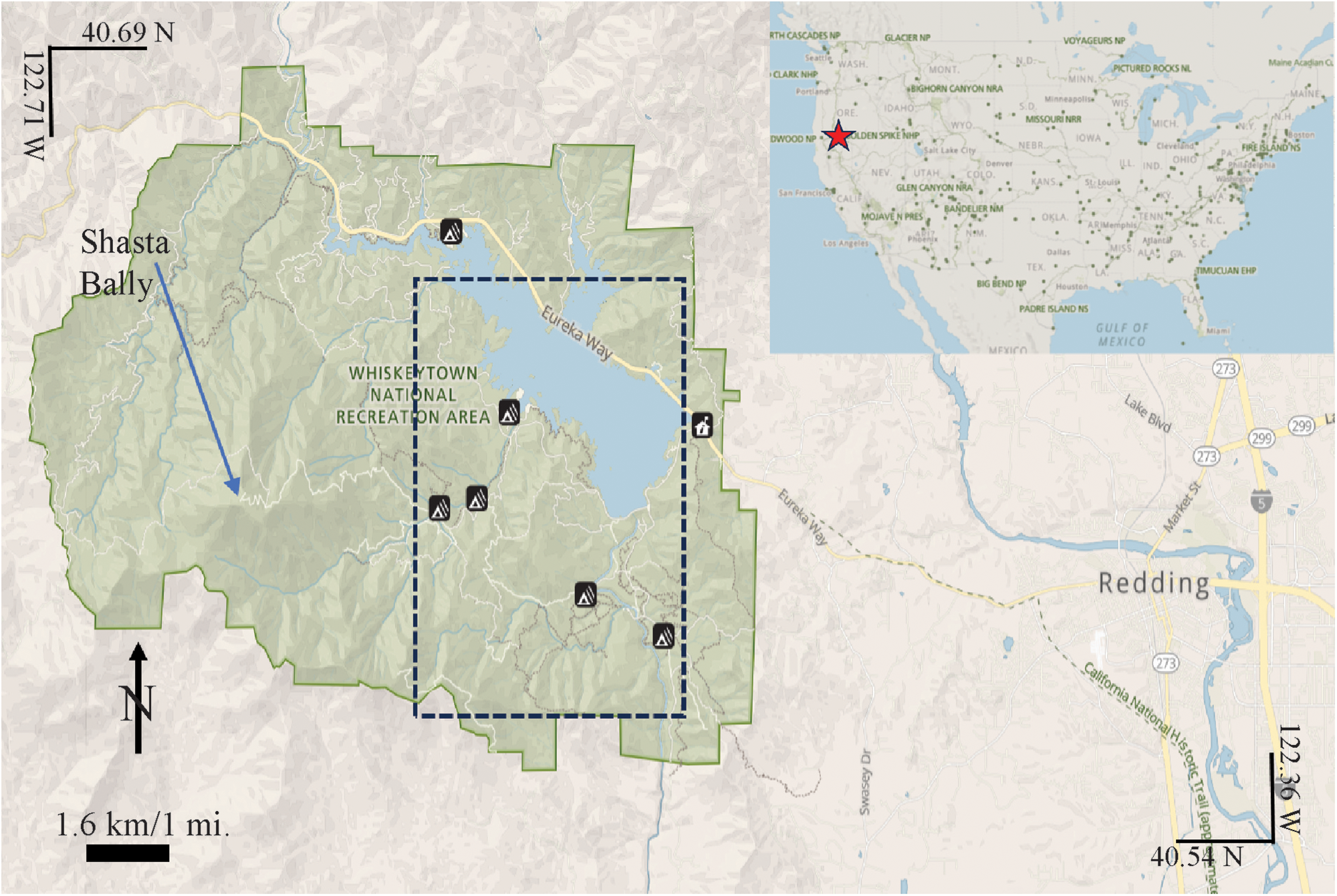
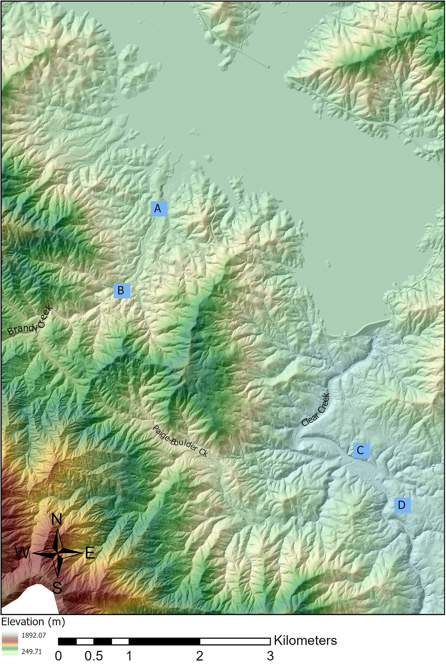
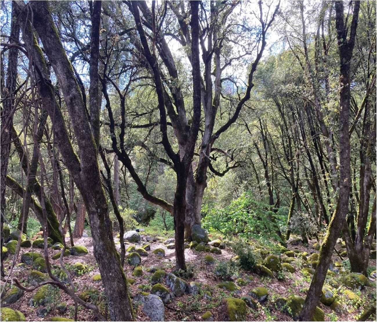
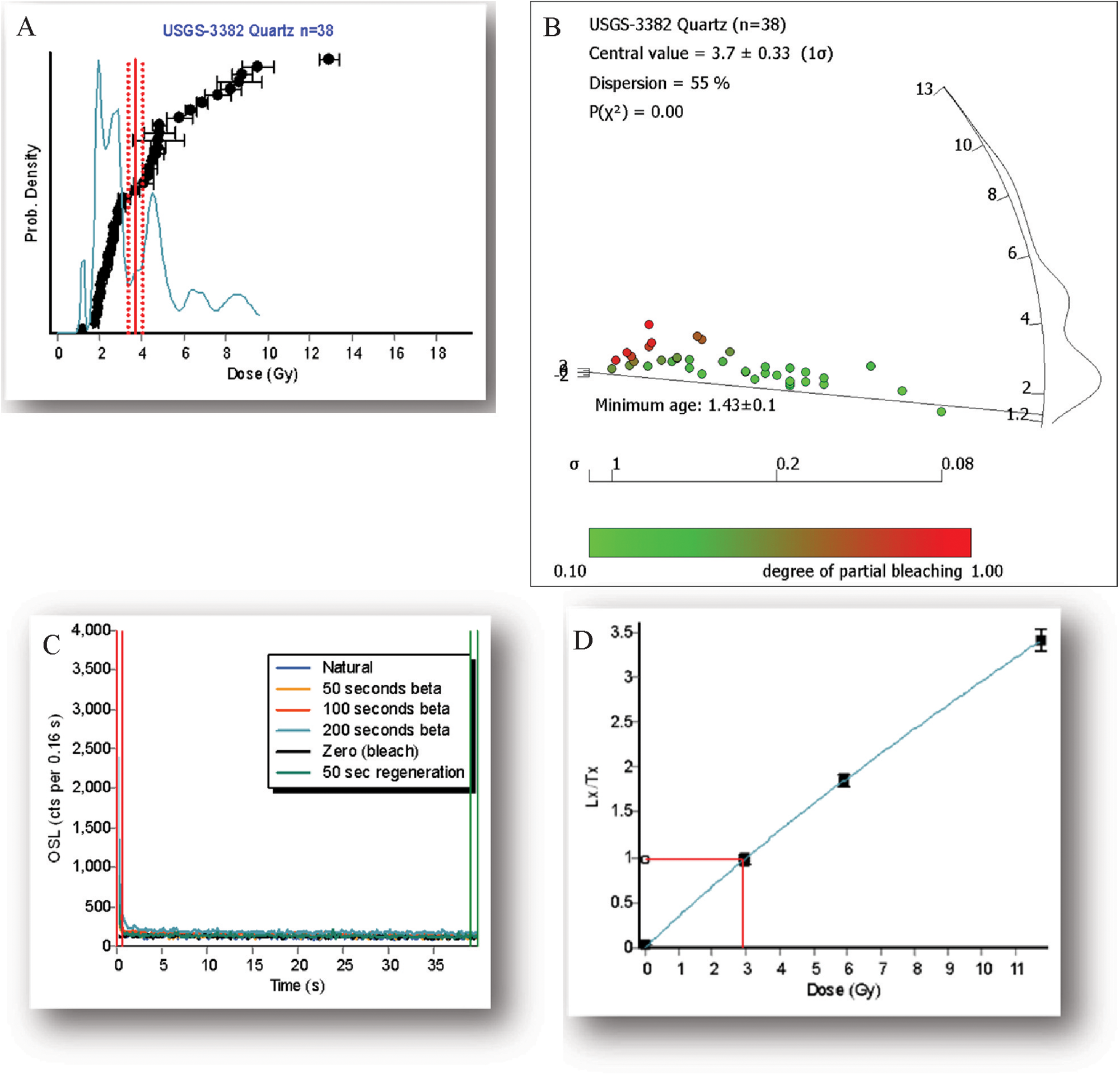
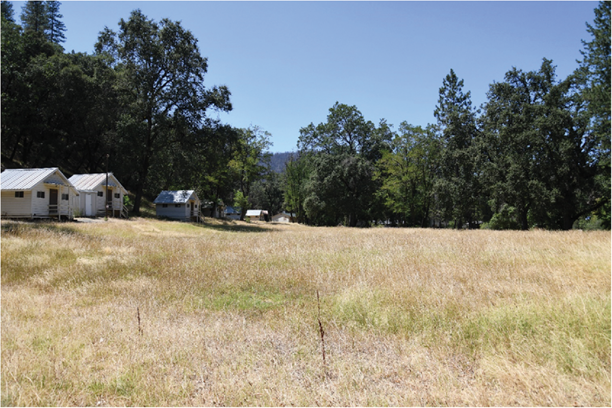
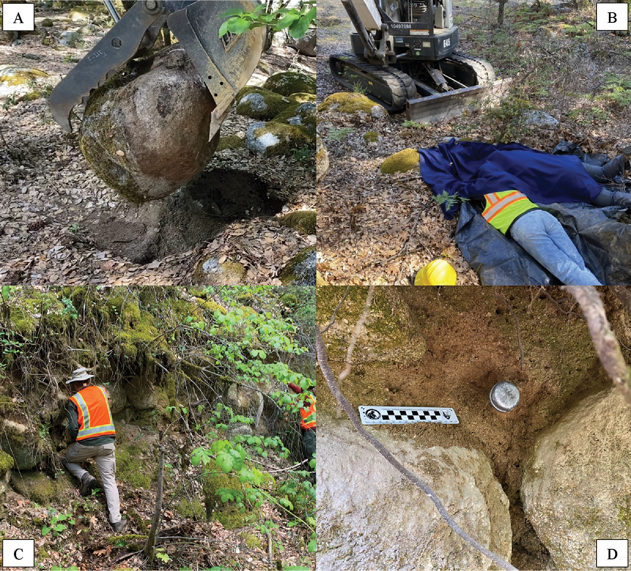
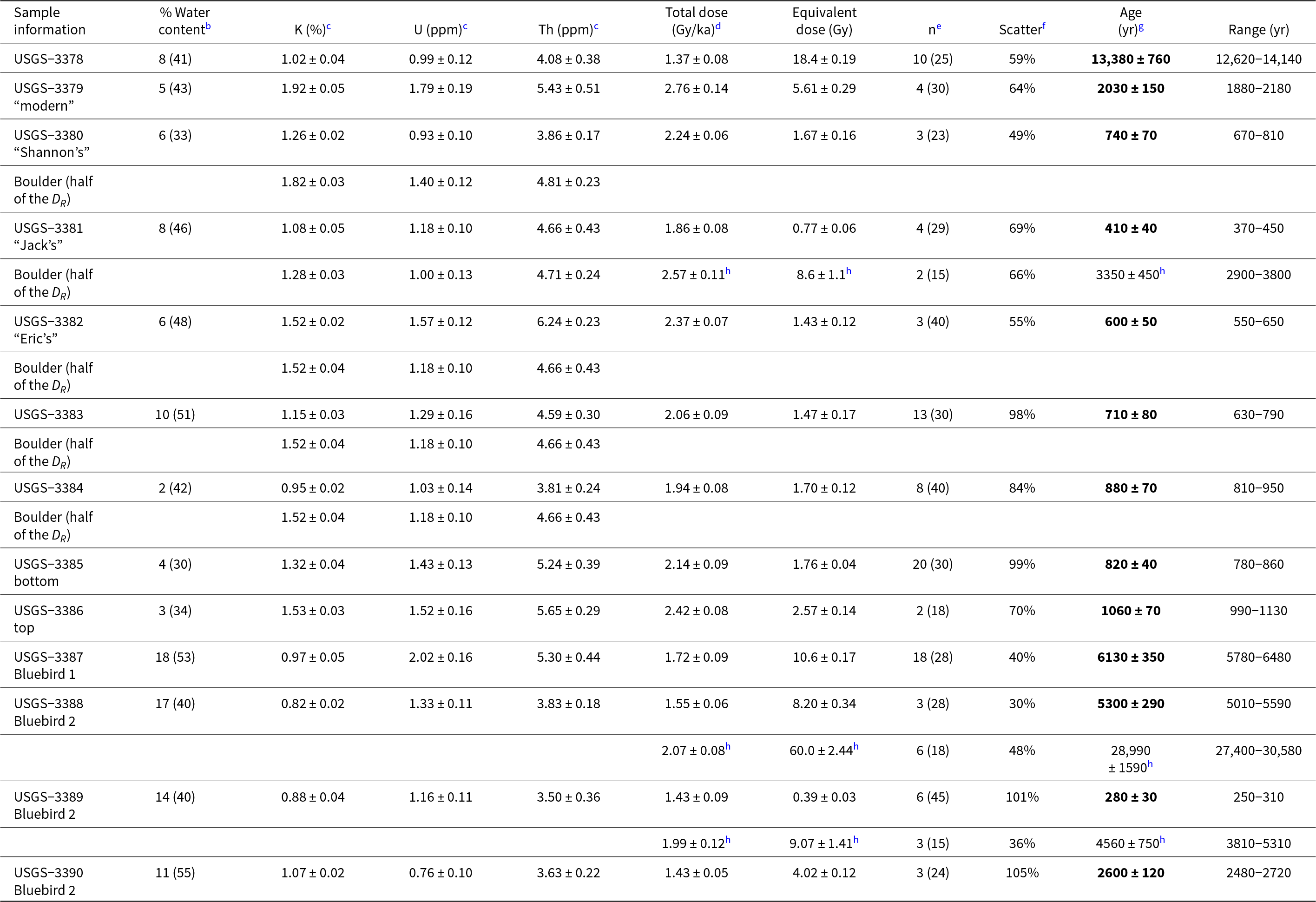
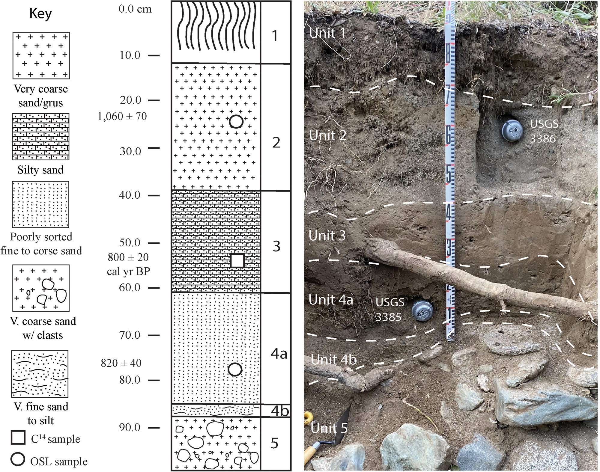
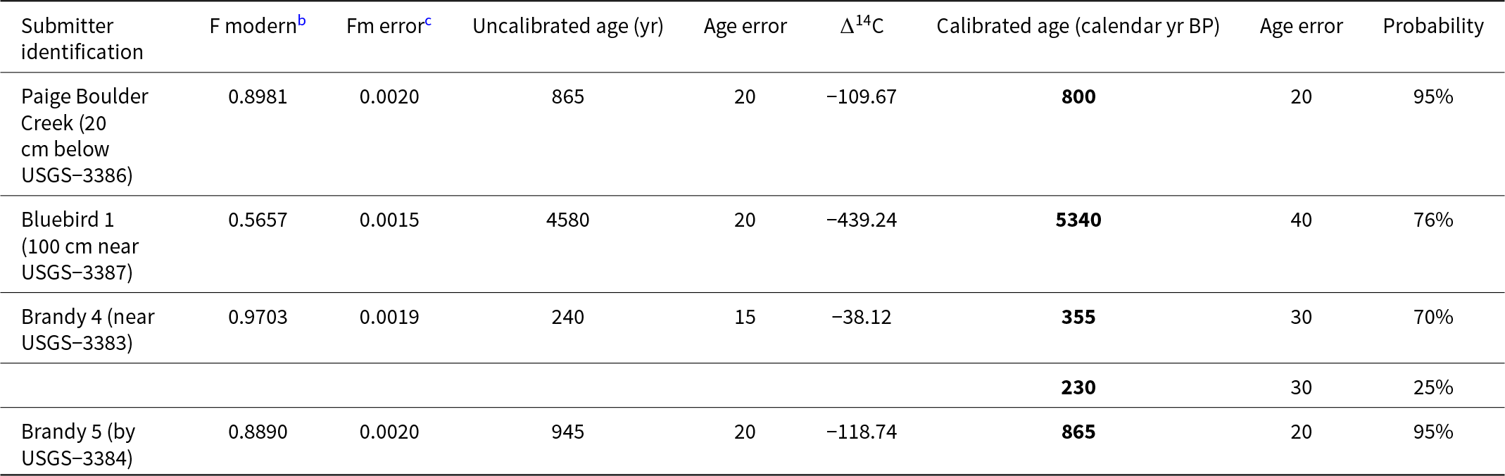
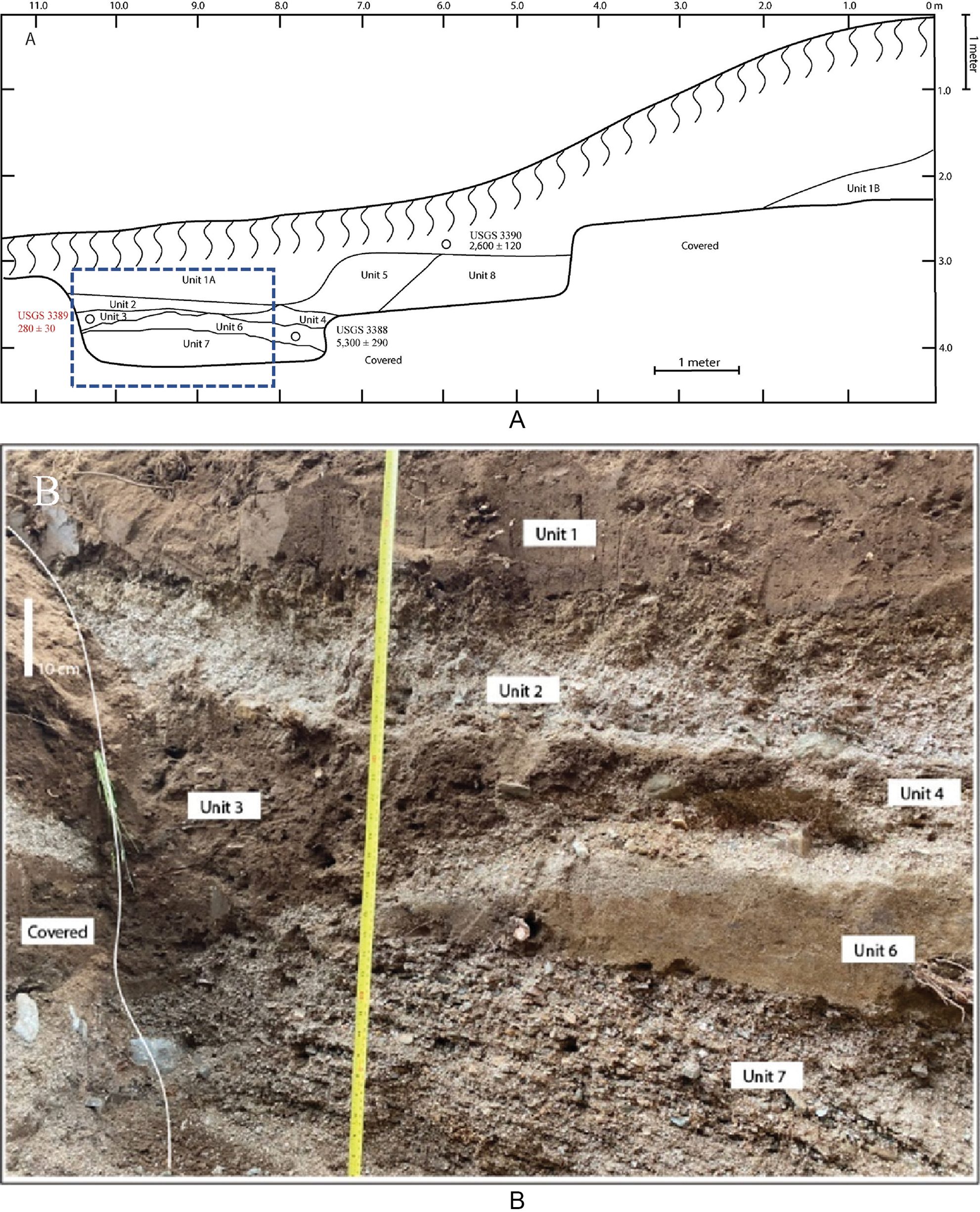
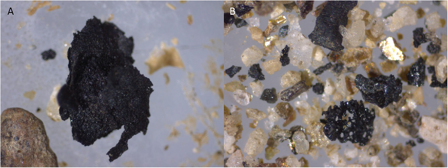


 Open access