


1. Introduction
During 1979–2021, the Arctic has warmed nearly four times faster than the global average (Rantanen and others, Reference Rantanen2022). The consequences of this accelerated warming are far-reaching, affecting weather extremes, the Greenland ice sheet, Arctic glaciers, ecosystems, marine biology, and human societies (Esau and others, Reference Esau2023). Arctic sea ice plays a pivotal role in both local and global climate systems, acting as a crucial climate indicator (Garcia-Soto and others, Reference Garcia-Soto2021). In recent decades, Arctic sea ice cover has undergone substantial transformations, characterized by record-low summer ice extent (Meier and others, Reference Meier2022), accelerated ice drift (Zhang and others, Reference Zhang, Pang, Lei, Zha, Zhao and Cai2022), and prolonged melt seasons (Markus and others, Reference Markus, Stroeve and Miller2009; Stroeve and others, Reference Stroeve, Markus, Boisvert, Miller and Barrett2014; Zheng and others, Reference Zheng, Cheng, Chen and Liang2021; Bliss, Reference Bliss2023).
The timing and lengthening of the melt season profoundly alter snow and sea ice thermodynamics by creating wet surface conditions in contrast to a frozen surface. Surface melting dramatically lowers the albedo (Perovich and others, Reference Perovich, Grenfell, Light and Hobbs2002), initiating and intensifying albedo feedback mechanism (Curry and others, Reference Curry, Schramm and Ebert1995; Zheng and others, Reference Zheng, Cheng, Chen, Wang, Liang and Wang2022). Earlier surface melt onset enhances solar radiation absorption at and below the ice surfaces in late spring, and in melt ponds, open leads, and open ocean areas during summer. The enhanced solar heating may further delay freeze-up onset in autumn (Stroeve and others, Reference Stroeve, Markus, Boisvert, Miller and Barrett2014; Steele and Dickinson, Reference Steele and Dickinson2016).
The timing of Arctic sea ice melt onset has been largely identified by remote sensing observations (Bliss and Anderson, Reference Bliss and Anderson2018). The physical drivers that impact the timing of Arctic sea ice melt onset were found in terms of the interannual variability of surface energy balance (Maksimovich and Vihma, Reference Maksimovich and Vihma2012), atmospheric moisture transport (Mortin and others, Reference Mortin, Svensson, Graversen, Kapsch, Stroeve and Boisvert2016), large-scale precipitation (Marcovecchio and others, Reference Marcovecchio, Behrangi, Dong, Xi and Huang2021) and atmospheric pressure patterns (Horvath and others, Reference Horvath, Stroeve, Rajagopalan and Jahn2021). Most previous studies have relied on individual datasets, whereas some (e.g. Smith and Jahn, Reference Smith and Jahn2019; Lin and others, Reference Lin, Lei, Hoppmann, Perovich and He2022) have included comparisons across multiple sources of data. However, melt onset between model and measurement has not been presented. Climate model results and observed snow depths (SDs) in the Arctic reveal a notable discrepancy in spring (Chen and others, Reference Chen, Liu, Ding, Zhang, Cheng and Hu2021; Webster and others, Reference Webster, DuVivier, Holland and Bailey2021). Differences in simulated and observed melt onset timing may contribute to this discrepancy. However, challenges remain in fully understanding the errors in the magnitude of melt onset in climate models and their underlying physical mechanisms.
The definition of melt onset varies depending on the research context and objectives of interest (Smith and Jahn, Reference Smith and Jahn2019). Cross-comparison on melt onset derived from in-situ and remote sensing observations as well as sea ice model simulations is crucial for identifying the physical mechanisms that determine the timing of melt onset. However, systematic comparison of modeled and measured melt onset has remained limited so far (Smith and Jahn, Reference Smith and Jahn2019), partly due to inconsistencies in snowmelt onset (SMO) definitions.
In this study, we investigate the surface melt onset on Arctic sea ice to identify the physical processes responsible for simulated biases to support model improvement. We focus on SMO rather than ice melt onset, as Arctic sea ice is typically snow-covered at the start of the melt season (Warren and others, Reference Warren1999). We apply a single-column thermodynamic snow and sea ice model (HIGHTSI) to simulate snow and ice mass balance (IMB) and temperature regimes along drift trajectories of 42 IMB buoys measured between 2010 and 2015. Modeling snow and sea ice along multiple IMBs drift trajectories is necessary because Arctic snow and sea ice exhibit large temporal and spatial variations (Kwok and others, Reference Kwok, Kacimi, Webster, Kurtz and Petty2020). The timing of SMO varies across individual locations, but the overall seasonality of SMO can be illustrated and assessed through a large ensemble of model experiments. In this study, we compare the modeled snow, ice thickness (IT), and temperature with IMB and passive microwave (PMW) remote sensing melt onset observations. Our objectives are (1) to validate the HIGHTSI modeled snow and ice thermodynamics against IMB observations; (2) to derive a new SMO definition based on modeled snow temperature profiles and to compare it with IMB observations; and (3) to quantify the difference among SMOs identified by IMB, HIGHTSI, and PMW datasets.
2. Data and methods
2.1. Ice mass balance (IMB) buoys
The IMB buoys (Richter-Menge and others, Reference Richter-Menge, Perovich, Elder, Claffey, Rigor and Ortmeyer2006; available at: https://imb-crrel-dartmouth.org/imb, last accessed 22 August 2025), developed by the MetOcean and the Cold-Regions Research and Engineering Laboratory (CRREL), represent a part of the Arctic drifting buoy network and have been deployed across the Arctic Basin since the 2000s to monitor SD and sea IT as well as vertical temperature profiles.
Each buoy was equipped with a thermistor string of 5 m in length. The thermistor sensors were mounted with 10 cm vertical resolution and their accuracy was ±0.1°C. The vertical temperature profile across the column of near-surface air, snow, ice, and the uppermost meters of the ocean was measured at a 2 hour (for the buoys pre-2010) or 4 hour (post-2010) sampling interval (Richter-Menge and others, Reference Richter-Menge, Perovich, Elder, Claffey, Rigor and Ortmeyer2006). Vertically embedded poles support two separate acoustic sounders: one facing downward (SR50A sonic rangefinder, deployed 1.5 m above the snow surface) to measure SD and surface melting, and one facing upward (PSA-916 sonar altimeter deployed below the ice bottom) to measure basal growth and ablation. Each IMB buoy was equipped with a GPS and a simple meteorological station to record the buoy position, near-surface air temperature, and barometric pressure. The sampling interval was typically 1 hour for GPS position, and the same interval as the temperature profile for acoustic sounders.
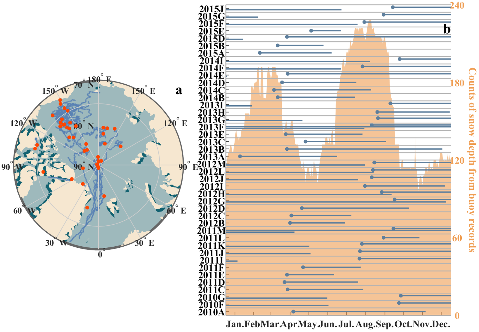
We utilized observations from 42 buoys deployed between 2010 and 2015 in various parts of the Arctic ocean. We ensured that all IMBs included in our model validations measured SD for at least 15 days. Figure 1 displays the buoys’ drift trajectories and operational durations, revealing predominant clustering within two major Arctic ice drifting patterns – the Beaufort Gyre and Transpolar Drift. The seasonal distribution of the count of recorded data points, exemplified by SD, exhibited a bimodal pattern. The highest peak occurred during August to September, following by a secondary peak around March to April.
(a) Drift trajectories of 42 ice mass balance (IMB) buoys used in this study. (b) Seasonal distribution of total snow depth sample counts (the Orange shadow) and lifespans of the buoys (the gunmetal gray bars), both presented at daily resolution.

Parameters measured by buoys – including SD, IT, snow/ice temperature (TS/TI) profile, near surface temperature, and GPS coordinates – were processed through the following procedures before being employed as either model inputs or validation benchmarks in this study. To remove noise and singular values, we applied regularizations to the recorded SD and IT time series. SD processing methodology was determined by the number of available measurements within a 2 day window centered in the middle (West and others, Reference West, Collins and Blockley2020). For time periods containing fewer than three measurements, linear interpolation was applied; when three or more measurements were present within the window of interest, a binomially weighted mean was applied. IT was processed by a moving quadratic fitting algorithm following the methodology of Lin and Zhao (Reference Lin and Zhao2019). The recorded TS and TI profiles were linearly interpolated to match HIGHTSI’s configuration – specifically, 10 layers in snow and 20 layers in sea ice. The snow surface, snow–ice interface, and ice bottom were used as reference levels (see Fig. S1 for details). The impact of thermistor string vertical resolution is illustrated in Supplementary Material (section S1).
2.2. Reanalysis data
ERA5 (available at: https://cds.climate.copernicus.eu/datasets/reanalysis-era5-single-levels?tab=download, last accessed 22 August 2025) is the fifth generation of the ECMWF (European Centre for Medium-Range Weather Forecasts) global reanalysis dataset, which provides comprehensive information on atmospheric, oceanic, and land-surface conditions (Hersbach and others, Reference Hersbach2020). The dataset covers the period from 1950 to the present and provides hourly data with high temporal and spatial resolution.
In this study, we used wind speed (10-m height), air temperature (2-m height), dew-point temperature (2-m height), cloudiness and snowfall rate to drive HIGHTSI. These hourly reanalysis variables were bilinearly interpolated along the IMB GPS coordinates.
2.3. Melt onset from PMW
The PMW-based SMO refers to the Arctic sea ice melt onset dataset developed by Markus and others (Reference Markus, Stroeve and Miller2009, available at: https://earth.gsfc.nasa.gov/cryo/data/arctic-sea-ice-melt, last accessed 22 August 2025). We specify this dataset as SMO, since Arctic sea ice is covered with snow before melt onset starts. This PMW-based algorithm determines SMO on the basis of weighted integration of three melt signature parameters: (1) the absolute difference in 37 GHz vertically polarized brightness temperature between adjacent days, (2) the absolute difference in ice concentration gradient ratio, and (3) independent melt/freeze thresholds. The brightness temperature was collected using the Nimbus-7 Scanning Multichannel Microwave Radiometer (SMMR), the Special Sensor Microwave/Imager (SSM/I) and the Special Sensor Microwave Imager/Sounder (SSMIS).
This dataset features a spatial resolution of 25 × 25 km and covers the temporal period from 1979 to the present. The dataset was categorized into early SMO (Early-SMO) and continuous SMO (Continuous-SMO). The Early-SMO is defined as the first day of melt occurrence, irrespective of the persistence of the signal, and the Continuous-SMO indicates the initial day of sustained summer melting. To enable inter-comparison, we extracted the Early-SMO and Continuous-SMO dates along the buoy trajectories. The PMW-derived SMO dates were determined for the location of each buoy at the time of surface melt onset detected in this study. Specifically, the Early/Continuous-SMO dates from the PMW grid cell corresponding to buoy-derived SMO dates were used.
PMW-derived SMO represents a suitable dataset for climate model evaluation. The primary uncertainties in this dataset emerged in the marginal ice regions in the Arctic (Bliss and others, Reference Bliss, Miller and Meier2017). Compared to another dataset of Arctic melt onset from Bliss (Reference Bliss2023), the melt onset differences between these two datasets were relatively smaller in the regions of interest in this study (e.g. the Central Arctic, Canadian Archipelago, Beaufort Sea, and Chukchi Sea).
2.4. HIGHTSI
We employed the HIGHTSI model, designed to simulate the evolution of mass balance and temperature variations in snow and sea ice in polar and sub-polar regions (Launiainen and Cheng, Reference Launiainen and Cheng1998). HIGHTSI has a moderate complexity in terms of solving snow and ice heat conduction, temperature, mass balance, as well as snow and ice interactions. This model has been applied extensively in modeling snow and sea ice in the Arctic Ocean (e.g. Cheng and others, Reference Cheng, Vihma, Zhanhai, Zhijun and Huiding2008; Yao and others, Reference Yao, Huang, Luo and Zhao2016; Merkouriadi and others, Reference Merkouriadi, Cheng, Graham, Rösel and Granskog2017; Reference Merkouriadi, Cheng, Hudson and Granskog2020). The energy budget at the surface is calculated as:
 \begin{align}&\left( {1 - {\alpha }} \right)\left( {1 - {e^{ - {\kappa _{s,i}}\Delta {h_{s,i}}}}} \right){{\text{Q}}_{sw}} + {Q_{lw \downarrow }}+ {Q_{lw \uparrow }}\left( {{T_{sfc}}} \right) \nonumber\\& + {Q_h}\left( {{T_{sfc}}} \right) + {Q_{le}}\left( {{T_{sfc}}} \right) + {F_c}\left( {{T_{sfc}}} \right) + {F_m} = 0,\end{align}
 where  ${Q_{sw}}$ is the incoming short-wave radiative flux,
  ${Q_{lw \downarrow }}$ is the downward longwave flux,
  ${Q_{lw \uparrow }}$ is the longwave radiation emitted by the surface.
  ${Q_h}$, and
  ${Q_{le}}$ are the turbulent fluxes of sensible heat and latent heat, respectively.
  ${F_c}$ is the surface conductive heat flux.
  ${\alpha }$ is the surface albedo,
  $\kappa $ is the extinction coefficient,
  $\Delta h$ is the thickness of the surface layer.
  ${T_{sfc}}$ is the surface temperature. The subscripts s and i denote snow and ice, respectively.
 ${F_m}$ is the heat flux due to surface melting:
 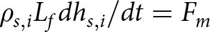 ${\rho _{s,i}}{L_f}d{h_{s,i}}/dt = {F_m}$.
  ${{\rho }}$ is the density of snow/ice,
  ${L_f}$ is the latent heat of fusion, h is the thickness of snow/ice, and t denotes the time dimension.
The  ${T_{sfc}}$ is solved by the Newton iteration method and used as an upper boundary condition for the partial differential heat conduction equation:
 \begin{equation}{\left( {\rho c} \right)_{s,i}}\frac{{\partial {T_{s,i}}\left( {z,t} \right)}}{{\partial t}} = \frac{\partial }{{\partial {\text{z}}}}\left[ {{k_{s,i}}\frac{{\partial {T_{s,i}}\left( {z,t} \right)}}{{\partial z}}} \right] - \frac{{\partial {q_{s,i}}\left( {z,t} \right)}}{{\partial {\text{z}}}},\end{equation}
 where T is the temperature, k is the thermal conductivity, c is the heat capacity.  $q\left( {z,t} \right) = \left( {1 - \alpha } \right){Q_{sw}}{e^{ - \kappa z}}$ is the amount of solar radiation penetrating below the surface layer. z represents the vertical coordinate (positive downward below surface).
The vertical distribution of solar radiation absorbed below snow or ice was calculated according to Grenfell and Maykut (Reference Grenfell and Maykut1977) and Perovich (Reference Perovich1996). The absorbed solar radiation contributed to both the heat balance of the surface layer and the warming of the internal snow and ice. Internal melting occurs when temperatures in one or more layers of snow or ice reach the melting point.
The lower boundary condition of (2) is described by the basal ice melt/growth:
 \begin{equation} - {\rho _i}{L_f}\frac{{d{h_i}}}{{dt}} = {\left. {\left( { - {k_i}\frac{{\partial {T_i}}}{{\partial z}}} \right)} \right|_{bot}} + {F_w},\end{equation}
 where  ${F_w}$ is the upward oceanic heat flux below sea ice.
  ${F_w}$ may reveal large spatial and seasonal variability in the Arctic Ocean (McPhee and others, Reference McPhee, Kikuchi, Morison and Stanton2003). Our modeling sensitivity study indicated it has the least impact on surface melting. In this study,
  ${F_w}$ is calculated based on the observed IMB energy budget (Lin and Zhao, Reference Lin and Zhao2019).
According to Equation (2), temperature variations within the interior of the snowpack are induced by vertical heat conduction between adjacent layers and the penetration of shortwave radiation into the snowpack. In addition to penetration of solar radiation below the snow surface, the effects of incident radiative and turbulent surface fluxes are transmitted to deeper snow and ice layers via heat conduction. Given the complexity of quantifying the nonlinear components of the conduction term, the modeled subsurface snow temperature change caused by conduction was calculated by:
 \begin{equation}d{T_{fc}} = d{T_{mol}} - d{T_{sw}},\end{equation}
 where  $d{T_{mol}}$ is the net modeled subsurface temperature change within a model time step (hour), and
  $d{T_{sw}} = \kappa \left( {1 - {\alpha _s}} \right){Q_{sw}}{e^{ - \kappa z}}\Delta t/\left( {{\rho _s}{c_s}} \right)$ is the modeled subsurface temperature change by shortwave radiation.
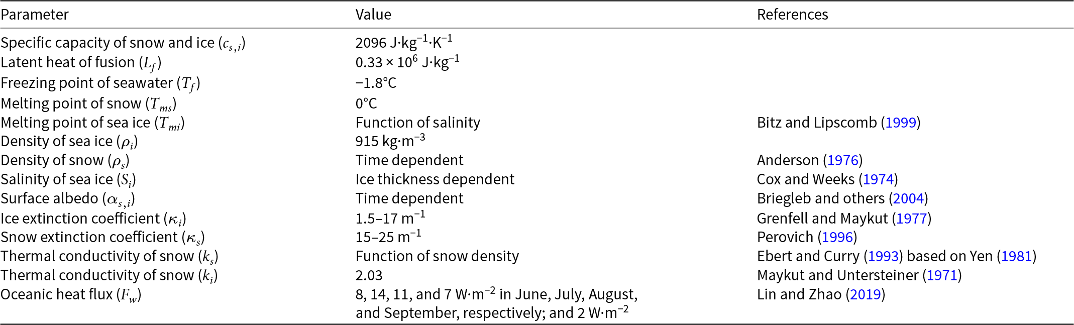
We initialized HIGHTSI based on IMB’s initial SD and thickness. Model runs applied using a Lagrangian approach along observed IMB drift trajectories and last until the end of the valid IMBs measurements. The modeled results are synchronized to buoy GPS positions for further analyses. Key parameters and parameterizations are summarized in Table 1.
Key parameters and parameterizations used in the standard HIGHTSI simulation.
2.5. Criterion to identify snowmelt events
Conducting direct SMO comparisons across models, observations, and remote sensing products is inherently challenging due to fundamental differences in their information content. The in situ-based SMO is typically determined by combining temperature and thickness measurements (West and others, Reference West, Collins and Blockley2020; Lin and others, Reference Lin, Lei, Hoppmann, Perovich and He2022). The sea ice model-based SMO has been determined based on TS/TI and phase change quantities (Smith and Jahn, Reference Smith and Jahn2019). In this study, we introduced two temperature-based SMOs that are relevant for both IMB observations and HIGHTSI simulations. The “surface-SMO” refers to the timing of the snowmelt event that occurred at the surface (the uppermost layer). The “subsurface-SMO” refers to the timing of the snowmelt event that happened in any snow layer (layers 2–10) below the surface.
The criterion for SMO is calculated as follows: (1) a 14 day sliding window is applied on IMB/HIGHTSI observed/modeled hourly TS at various layers; and (2) if the obtained moving average TS is larger than −1°C, the surface-SMO or the subsurface-SMO is identified. The “−1°C” is consistent with the temperature-based surface melt onset by Bliss and Anderson (Reference Bliss and Anderson2018) and Rigor and others (Reference Rigor, Colony and Martin2000), where the daily temporal resolution data were applied. This criterion facilitates the quantification of IMB/HIGHTSI-based SMOs, the inter-comparison of modeled and observed SMOs, and statistical analyses.
3. Results and discussions
3.1. Snow depth, ice thickness, and temperatures
To quantify the fidelity of seasonal simulations, we first present results of a systematic comparison of primary model outputs (SD, IT, TS, and TI) against observations. The comparison is organized as follows: For each single day of year, we extracted all hourly SD, IT, TS, and TI data points derived from both model and IMB corresponding to this calendar day. The collected data then were averaged for each day of year to produce a seasonal evolution of these variables (Fig. 2a–d). For each calendar day, the daily mean values incorporated data along the drift trajectories of all buoys whose lifespans included that specific day.
Observed (Obs.) and Modeled (Mol.) time series of (a) snow depth, (b) ice thickness, (c) vertically mean snow temperature, (d) ice temperature, and (e) air temperature. The lighter shadows indicate the daily standard deviation across multiple buoys for each series on each day.
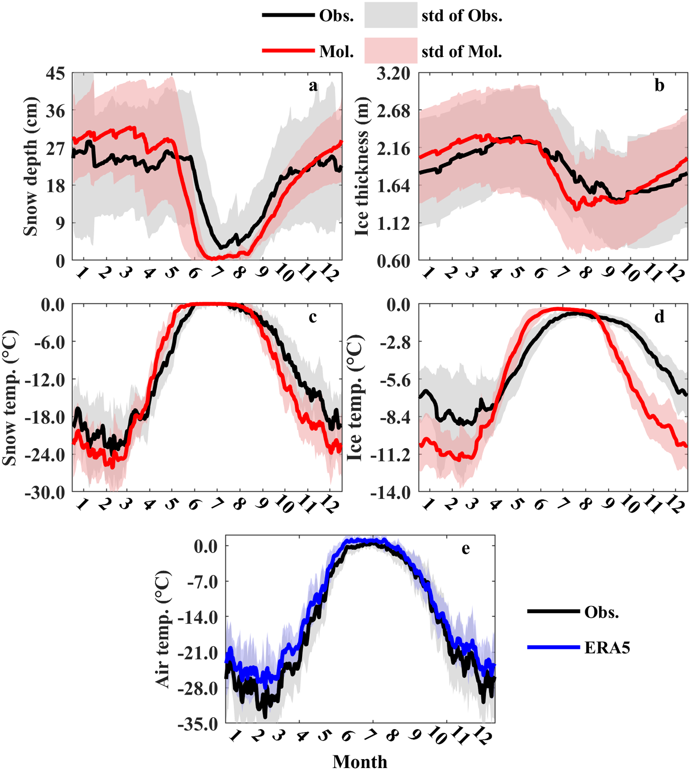
The observed SD exhibited variability from December to June, maintaining fluctuations around approximately 25 cm (Fig. 2a). A rapid decline started in June, attainting its seasonal minimum (∼5 cm) by July. Subsequently, heavy accumulation occurred from August through November, re-establishing the winter snowpack. HIGHTSI exhibited distinct seasonal biases in SD simulation: a positive bias of 3 ± 4 cm during October–April, contrasting with a negative bias of −5 ± 4 cm in May–September. Notably, the modeled SD initiated its rapid decline in May – about 1 month earlier than observed. A more rigorous analysis of this error will be provided in Section 3.2.
Despite the premature SMO, the model demonstrated a snowmelt rate that was comparable to the observed one: −0.58 cm·day−1 from days 134 to 182 for the model results, and −0.53 cm·day−1 from days 162 to 200 for IMBs). Also, the ERA5-based snow accumulation rate during stable cold conditions (0.27 cm·day−1 during days 225–295) well matched the one detected by the IMBs (0.26 cm·day−1 during days 225–295). These results suggested that the model captures the snow melting and accumulation rates in spring and autumn compared to observations. However, the onset of melt was triggered too early in May and snow accumulation persisted beyond December.
The modeled mean IT exhibited seasonal variations similar to SD, underestimation in summer and overestimation in winter (Fig. 2b). The differences between the modeled and the measured IT were denoted as 0.14 ± 0.09 m from October to April and −0.15 ± 0.15 m from May to September. The modeled sea ice melted at the rate of −18 mm·day−1, which was 2.7 times than the observed rate (from days 164 to 214 for model, and 164 to 239 for IMBs). The model also overestimated the growth rate of ice during autumn and the early winter, with the value of 6 mm day−1 for model and 3 mm day−1 for observation (from days 288 to 365 for both). Both the daily standard deviations of the modeled and observed snow and ITs were large, approximately on the same order of magnitude as their daily averages. This indicates considerable spatial variations in snow and ice across the Arctic.
Both modeled TS and TI exhibited consistent cold biases during October–April and warm biases during May–September relative to the measured values (Fig. 2c and d). The mean differences were approximately 0.4 ± 2.0°C for Ts and 0.5 ± 1.2°C for TI in the warm months (snow-free conditions were excluded from the calculations), and −2.7 ± 2.4°C for Ts and −3.0 ± 1.4°C for TI in the cold months. The modeled rates of temperature change tended to be overestimated compared to measurements. For instance, the modeled warming rate of TS was 0.32°C·day−1 between days 72 and 145 (prior to the deceleration of TS increase as it approaches the melting point), while the recorded rate for the same period was 0.25°C·day−1. A precipitous decline in modeled temperatures was also noticed at the transition between summer and autumn for both TS and TI. This may explain the good agreement of observed and modeled IT in May and October (Fig. 2b): pre-May cold biases offset the post-May warm biases, and pre-October warm biases offset post-October cold biases.
There were notable discrepancies between modeled and recorded TI in both the timing and duration of the high-temperature occurrence near the melting point. Nevertheless, the daily temperature variations in model and measurement were highly correlated. From May to September, the correlation coefficients between two series were 0.73 for TS and 0.62 for TI, respectively; while in winter, they were 0.88 for TS and 0.78 for TI. Based on the daily standard deviations of TS and TI across multiple buoys shown in Fig. 2, the differences in TS and TI between buoys remained substantial in winter, but were much smaller in the warm months.
The model-observation discrepancies likely arise from either (1) biases in the forcing data or (2) unresolved physical processes in the model. Given the scarcity of large-scale and long-term observational data and the assimilation of available observations in reanalysis datasets, it is a challenge to conducting a comprehensive and detailed verification of the parameters in these datasets. The widespread availability of in-situ temperature data has enabled extensive validation of ERA (Wang and others, Reference Wang, Graham, Wang, Gerland and Granskog2019; Demchev and others, Reference Demchev, Kulakov, Makshtas, Makhotina, Fil’Chuk and Frolov2020; Herrmannsdörfer and others, Reference Herrmannsdörfer, Müller, Shupe and Rostosky2023; and also Fig. 2e in this study). These studies consistently identified warm biases in ERA5’s representation of air temperature in the Arctic Basin, partly attributed to its missing representation of snow cover over sea ice (Batrak and Müller, Reference Batrak and Müller2019). In addition to ERA5, this has contributed to near-surface warm biases in all ECMWF products over decades both in the Arctic and Antarctic sea ice zone (Vihma and others, Reference Vihma, Uotila, Cheng and Launiainen2002; Jakobson and others, Reference Jakobson, Vihma, Palo, Jakobson, Keernik and Jaagus2012). The winter cold biases in modeled TS and TI (Fig. 2c and d) – despite ERA5’s proved warm bias in air temperature relative to measurement (Fig. 2e) – may stem from inadequate snowpack insulation in HIGHTSI. This deficiency leads to excessive heat loss from the snow-ice system to atmosphere, overriding the compensating effect of ERA5’s overly warmer near-surface temperature.
The mismatch in winter SD variability between HIGHTSI and IMBs (Fig. 2a) may be explained by the model’s limited ability to represent dynamic snow processes in the cold season, such as wind-driven blowing snow (Liston and others, Reference Liston2020). ERA5’s potential overestimation of snowfall may be responsible for the uncertainty to snow accumulating simulations in the cold seasons (Avilada-Diaz and others, Reference Avilada-Diaz, Bromwich, Wilson, Justino and Wang2020).
The temporal distribution of buoy observational data, as shown in Fig. 1b, reveals a scarcity of samples during the months of May, June, November, and December. These gaps in observational coverage highlight the need to more additional in situ deployment during these critical periods. Increasing observations in late spring can provide valuable insights into the transition from freezing to melting, which is crucial for improving model accuracy in simulating melt onset of snow and ice. Similarly, expanding data coverage in November and December will support a better understanding of early winter freezing processes, including the thermal and mechanical responses of snow and ice to alteration of environment forcing.
3.2. SMO simulation
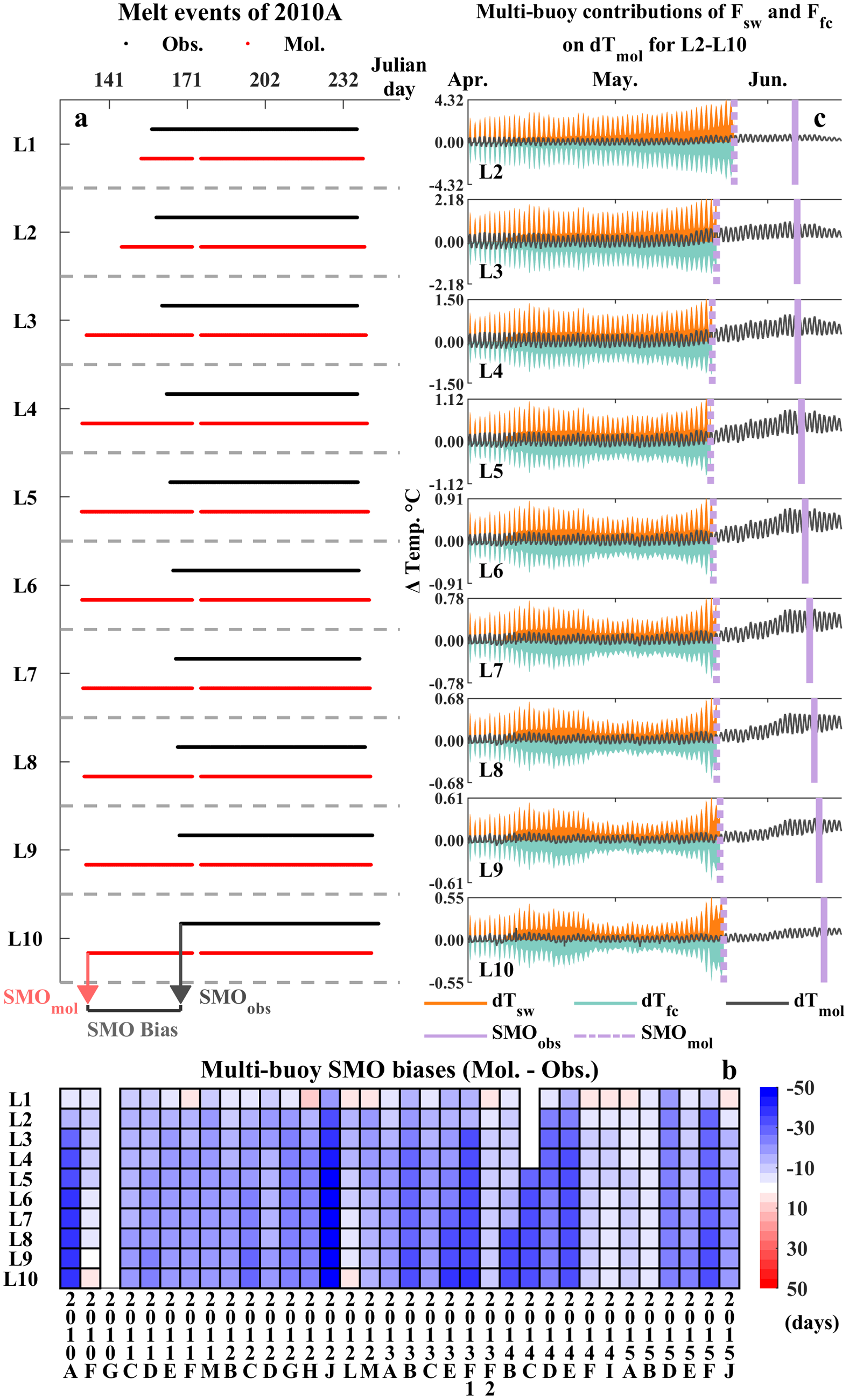
Disparities in snow between HIGHTSI and IMBs during in early melt stage will be discussed in this section, focusing on quantitative analyses on SMO. Following the method introduced in Section 2.5, we obtained snowmelt event sequences for Layer 1–10 and SMOs from HIGHTSI and IMBs (exemplified by 2010A in Fig. 3a). By subtracting the observed SMO from the modeled SMO, we analyzed the SMO differences between HIGHTSI and IMBs across 34 buoys. The 34-buoy subset was selected based on their temporal coverage of the initial melting stage, which the others lacked. In this section, the term “multi-buoy average” refers to the average over the data from these 34 buoys.
(a) Snowmelt events identified using the temperature threshold of −1°C for observations (black) and HIGHTSI (red) across 10 snow layers for buoy 2010A. L1 denotes the surface layer, and L10 denotes the snow/ice interface; (b) Differences in SMO between observations and HIGHTSI. Buoy 2013F experienced two melting periods. A blank value indicates either a lack of identified observed melt events (2010G and 2014I) or missing temperature measurements (2014C); (c) Modeled snow temperature change (dT mol) at L2–10 (note the larger range of the y-axis values in the upper layers), along with the contributions of solar radiation penetrating into snow (dT sw) and vertical heat conduction (dT fc), averaged over 34 buoys from April 1st to June 15th. The vertical pale purple dashed line represents the modeled SMO, while the solid line represents the observed SMO.

The SMO differences between model and measurement are shown in Fig. 3b. The surface layer (L1) typically revealed an early modeled surface-SMO compared to observations, while the deeper layers (L2–10) showed more pronounced differences. The surface layer showed modest mean SMO differences with −5 ± 6 days (negative gives an earlier SMO in the model), which could be attributed to the high sensitivity of the surface layer to external environmental changes. While the subsurface layers displayed notably earlier modeled subsurface-SMO (−18 ± 3 days on multi-buoy average across L2–10).
The vertical gradient of modeled SMO profile failed to replicate the pattern from IMBs (Fig. 3c) on multi-buoy average. The observed SMO profile at L2–10 showed a consistent gradient in the delay of SMOs with increasing depth at 16 hours per layer. In contrast, the modeled SMO profile exhibited a C-shape pattern: L2–4 demonstrated an advancing variation with increasing depth at −36 hours per layer (+4 hours per layer for IMBs at L2–4), while L5–10 revealed a progressively delayed SMO variation of 11 hours per layer (+18 hours per layer for IMBs at L5–10). This may imply that the distribution of modeled heating rates among layers from the middle to the bottom of the snowpack is rather reasonable.
In a short summary, compared to IMBs’ SMOs, the model exhibited remarkable earlier subsurface-SMO timing rather than surface-SMO. Using the methodology described in Section 2.4, we decomposed the net modeled temperature change in L2–10 into contributions from shortwave radiation absorption and conductivity heat flux as a first step toward understanding the possible caused of these subsurface-SMO biases. Fig. 3c illustrated the temporal variations of these variables for the subsurface snow layers (L2–10) across multiple buoys from April 1st to June 15th. The decomposing analysis revealed that shortwave radiation is the only heating factor contributing positively to the temperature increase during this period, while the conduction term consistently served as a cooling factor. This ruled out the possibility that the upper subsurface layers, such as L2, were over-heated by the surface layer through conduction. Since the shortwave term represented a more active role compared to the passive nature of conductive heat transfer, we attributed the primary cause of the temperature modeled subsurface-SMO to an overestimation of solar radiation – either due to an overestimation of the solar absorption in snow or underestimated surface albedo.
To demonstrate the inaccuracy caused by forcing, we executed an additional HIGHTSI run, in which the ERA5 2-m air temperature was replaced by the 2-m air temperature from IMBs as the atmospheric input. To our knowledge, the buoy data were not assimilated into the ERA5 reanalysis product. ERA5 air temperature exhibited consistent warm biases relative to measurements throughout the annual cycle, with mean deviations of 1.2 ± 1.9°C in the warm season and +2.9 ± 3.9°C in the cold season (Fig. 2e). Experiment replacing ERA5 with recorded air temperatures yielded two key outcomes (Fig. S2): (1) a reduction in positive temperature biases in warm season (e.g. the positive bias of TS reduced from 0.5°C to 0.2°C), but an slightly amplification of cold season negative (TS error increased from −2.7°C to −2.8°C); and (2) improved but still non-negligible SMO biases, where multi-buoy averaged discrepancy were reduced to +3days for surface-SMO yet remained substantial at −14 days for subsurface-SMO. These results demonstrated that while correcting atmospheric forcing addressed surface temperature adjustment by altering turbulent heat flux, its impact on subsurface snow layer was limited to reducing upward conductive heat losses (as discussed in the paragraph above). We attributed the persistent premature internal snowmelt primarily to excessive shortwave radiation penetration.
Given the potential limitations of our SMO estimation method described in Section 2.5, we performed sensitivity tests by varying the sliding-average window and the criteria used to detect snowmelt events. Across L1–10, three alternative criteria were applied to the sliding-averaged TS series with window of 2, 7, and 14 days (used in the former analysis), respectively. The criteria were Criterion 1: The sliding-averaged TS should ≥−1°C at the time of interest (used in the former analysis); Criterion 2: TS ≥ −1°C and the daily HS variation must be negative; and Criterion 3: TS ≥−2°C and the HS should be in decreasing (West and others, Reference West, Collins and Blockley2020). The results revealed that the selection of temporal averaging windows and snowmelt determination criterion during preprocessing primarily influenced the magnitude of SMO bias estimates, while exerting minimal impact on the study’s general conclusions regarding earlier modeled SMO than observations (Fig. S3).
3.3. Inter-comparison of SMO based on IMBs, HIGHTSI, and PMW
Building upon the comprehensive IMBs-HIGHTSI comparison of SMO in Section 3.2, we incorporated the widely used PMW-derived Arctic melt onset product to conduct a tripartite validation framework among IMBs-HIGHTSI-PMW. This multi-scale analysis enabled evaluation of the same parameter (melt onset) across different definitions.
Given the predominant presence of snow cover on sea ice in the beginning of the Arctic melt season, we assumed PMW-derived melt onset as representing the timing of surface snowmelt. Consequently, our inter-comparison with PMW melt onset in this section utilized exclusively the surface-SMO from IMBs and HIGHTSI discussed in the former section. This alignment ensured consistent SMO comparison at the surface level.
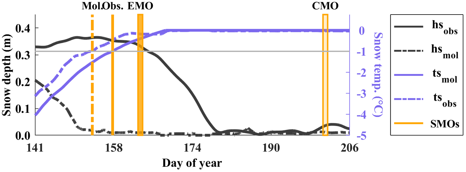
We presented SMOs comparison among the mentioned datasets for Buoy 2010A as a case study (Fig. 4). During the critical melting period (days 140–165), the modeled TS at surface generally tracked the recorded temperature evolution, albeit with a persistent warm bias of ∼0.7°C. This temperature discrepancy resulted in 4 day advancement in modeled surface-SMO relative to measurement. Notably, the surface-SMO from 2010A coincided precisely with the onset of rapid SD decline, validating the SMO detection methodology used in prior analyses. While the 4 day surface-SMO difference appeared modest, the model exhibited substantially earlier snowmelt in SD. Insights from Fig. 3b suggested that the subsurface snowmelt earlier than surface created this SD bias between HIGHTSI and IMB. The PMW-derived Early-SMO and Continuous-SMO occurred approximately 5 and 43 days later than the observed SMO at surface, respectively. The melt onset determined by Early-SMO demonstrated reasonable reliability in this case study, while the Continuous-SMO yielded substantially delayed timing – typically occurring after the complete ablation of the observed snow cover.
Example of the surface-SMOs from IMBs (Obs.), HIGHTSI (Mol.), PMW-derived Early-SMO (EMO in the legend), and Continuous-SMO (CMO in the legend) during the melt season, exemplified by 2010A. The black lines represent observed (solid) and modeled (dashed) snow depths, the lavender lines denote the sliding-averaged snow temperatures at surface, and the Orange lines mark the SMOs. The horizontal gray line indicates the −1°C threshold, with surface-SMO from IMBs and HIGHTSI determined by the intersection point between this line and the temperature series.
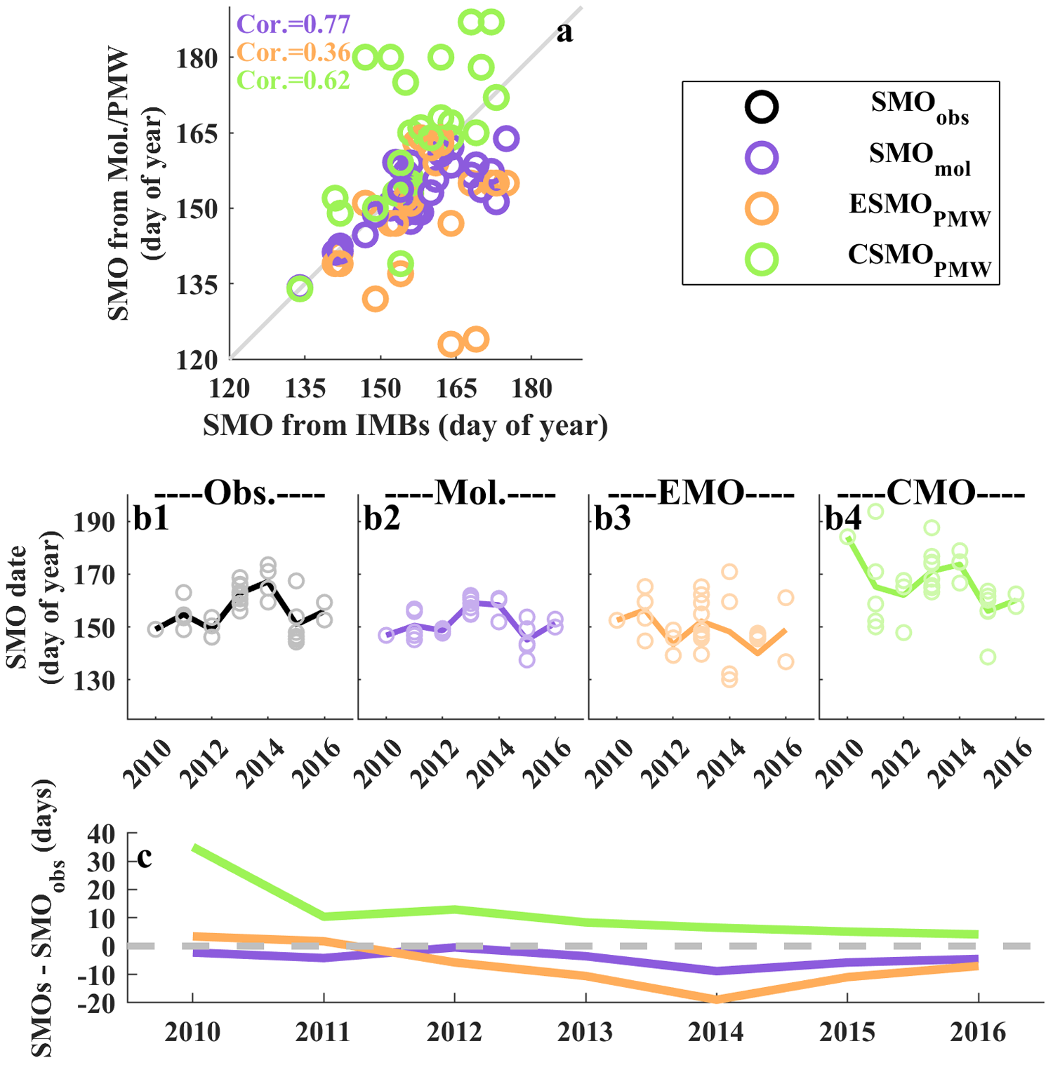
Scatterplot comparison between surface-SMOs form measurements and SMO from model, and Early- and Continuous-SMO PMW across 34 IMBs were presented in Fig. 5a. Consistent with prior analyses, HIGHTSI generally produced premature surface-SMO across most buoys, with a multi-buoy mean advancement of 5 ± 6 days relative to IMBs. Similarly, PMW-derived Early-SMOs tended to occur earlier than observed, whereas Continuous-SMOs were generally delayed. The multi-buoy average errors for Early- and Continuous-SMOs were −12 ± 20 days and 5 ± 22 days, respectively. For the PMW-derived SMOs along the buoy trajectories utilized in this study, the average time gap between Early- and Continuous-SMOs was approximately 1 week.
(a) Scatter plots of surface-SMO dates from IMBs versus those derived from HIGHTSI, and PMW (Early- and Continuous-SMO). (b1–b4) Inter-annual variations in SMO derived from the datasets after latitudinal detrending. (c) Differences in the inter-annual variations of SMOs from HIGHTSI, PMW-derived Early- and Continuous-SMO relative to IMBs.

Characterizing the inter-annual variability of the SMO is essential for understanding the climate change we are currently experiencing. However, as established in prior studies (e.g. Lin and others, Reference Lin, Lei, Hoppmann, Perovich and He2022), melt onset exhibited a strong latitude dependence. Consequently, direct comparisons of inter-annual variability among the SMOs may be confounded by spatial (latitudinal) biases. To mitigate this effect, we removed the latitudinal trend from the SMO datasets used in this study (Fig. S4, exemplified by SMOs from IMBs). The subsequent analyses of inter-annual variability in this section were all based on the detrended results.
The inter-annual variations from the four datasets were shown in Fig. 5b1–b4. Although the study period was too short to establish a statistically robust inter-annual trend, certain consistent patterns emerged across all SMO dataset. In 2015, all surface-SMOs exhibited a pronounced and synchronous advancement compared to 2014. The model demonstrated the smallest discrepancies among all datasets in the inter-comparison, followed by Early-SMO from PMW. In contrast, the Continuous-SMO displayed the largest deviations, particularly in 2010–2011. Correlation analyses further confirmed that the surface-SMO from HIGHTSI aligned closely with observations, yielding a high correlation coefficient with 0.94. In comparison, Early- and Continuous-SMO from PMW showed weaker correlation with 0.26 and 0.19, respectively. However, an apparent improvement in correlation between Continuous-SMO and observations was evident starting 2012.
4. Conclusions
A single-column model was used to simulate snow and sea ice thermodynamics along the drift trajectories of 42 IMBs between 2010 and 2015, focusing on SD, IT, their temperature regimes, and the timing of SMO. The simulated average SD, IT, and TS/TI qualitatively captured the observed seasonal variations. The HIGHTSI modeled and IMB observed surface-SMO revealed a good inter-annual correlation during the IMB operation period addressed in this study (2010–2016). The modeled average surface-SMO preceded the observed one by 5 days.
The PMW based Early-SMO and Continuous-SMO are widely used surface melt onset products in Arctic climate research and as climate indicators. Our cross-comparison reveals that despite discrepancies in spatiotemporal scales and melt onset definitions, the PMW-derived Early-SMO occurred 12 days before the IMB-derived surface-SMO, while the PMW-derived Continuous-SMO showed a 5 day lag. Further analyses based on the satellite-derived brightness temperature and top-of-atmosphere signals simulated by radiative transfer models are needed to better determine physical mechanisms responsible for the satellite-derived SMO discrepancies.
The differences between modeled and observed subsurface-SMO are larger than those of the surface-SMO. The largest differences occur at the lower subsurface snow layer, where modeled SMO exceeds the observations by up to 18 days. Using measured air temperature as forcing for HIGHTSI reduces the discrepancy in modeled subsurface-SMO by 5 days. We speculate that the subsurface-SMO is driven by penetrating solar radiation, and therefore in-snow temperature profile, in contrast to the surface-SMO, which is largely driven by downward longwave radiation, largely originating from warm clouds (Maksimovich and Vihma, Reference Maksimovich and Vihma2012).
The model bias toward too early subsurface-SMO may be caused by an overestimation of absorbed solar radiation. Further evaluation and improvement of the radiative transfer processes in snowpack is needed for more accurate modeling of SMO.
Supplementary material
The supplementary material for this article can be found at https://doi.org/10.1017/aog.2025.10023.
Data availability statement
The respective repositories for the primary data used in this study are listed in Section 2 (Data and Methods). The computed and modeled data supporting the findings of this study are available from the first/corresponding author upon request.
Acknowledgements
H. Yin and J. Su are supported by the Laoshan Laboratory Technology Innovation Project (No. LSKJ202202301), the National Key R&D Program of China (No. 2023YFC2809101), the National Natural Science Foundation of China (No. 42076228). L. Lin are supported by the Natural Science Foundation of Shanghai (No. 22ZR1468000). B. Cheng and T. Vihma were supported by European Union’s Horizon2020 research and Innovation Framework Programme PolarRES project (No.101003590). B. Cheng was also supported by the Research Council of Finland project IceScales (grant n. 364939).
Competing interests
The authors declare that they have no known competing financial interests or personal relationships that could have appeared to influence the work reported in this paper.


 Open access