


1. Introduction
The evolution of a wake in a stratified environment has garnered much attention since the early work by Lin & Pao (Reference Lin and Pao1979), and reviews of the literature can be found in Spedding (Reference Spedding2014) and de Bruyn Kops & Riley (Reference de Bruyn Kops and Riley2019). Two model problems that have been studied extensively numerically are temporally evolving wakes and spatially developing wakes in a linearly stratified environment, which are sketched in figures 1 and 2. The spatial coordinate  $x$ in figure 1(a) and the time coordinate $t$ in figure 1(b) are interchangeable according to $x=U_bt$, where $U_b$ is the convective velocity. Simulations of spatially evolving wakes necessitate the concurrent resolution of both the near wake and the far wake. On the other hand, simulations of temporally evolving wakes require only the wake characterization at a specific time. Consequently, when investigating the late wake, simulations of temporally evolving wakes are often more straightforward than simulations of spatially developing wakes (Chongsiripinyo & Sarkar Reference Chongsiripinyo and Sarkar2020). Nevertheless, the initialization of temporally evolving wake simulations remains challenging practically, unless calculations of a spatially evolving wake at the same flow condition are readily available (Pasquetti Reference Pasquetti2011; VanDine, Chongsiripinyo & Sarkar Reference VanDine, Chongsiripinyo and Sarkar2018).
Schematics of stratified wake flows. (a) A spatially developing wake in (i) the streamwise vertical plane and (ii) the streamwise transverse plane. (b) A temporally evolving wake in (i) the streamwise vertical plane and (ii) the streamwise transverse plane. The fields are from case R20F02 at  $Nt=4.5$, 52, 110 and 400, which will be detailed in § 2.

(a) Visualization of the instantaneous vertical vorticity field  $\omega _z$ on the horizontal plane $z=0$. (b) Instantaneous spanwise vorticity field $\omega _y$ on the vertical plane $y=0$. Four snapshots are at $Nt=4.5$, 52, 110 and 400, respectively. The fields are from case R20F02.

Significant insights have been gained into the flow physics of stratified wakes since the seminal work of Lin & Pao (Reference Lin and Pao1979). Here, we provide a brief overview of the basic flow phenomenology. First, we define the local Froude number  $Fr=U_0/(NL)$, where $L$ is an integral length scale, $U_0$ is the centreline velocity deficit, and $N$ is the Brunt–Väisälä frequency. The local Froude number describes the competition between the inertial and buoyancy forces. In many real-world scenarios, such as the wake behind an underwater vehicle in the deep sea, Froude numbers start off large, gradually decrease as the wake decays, and eventually reach order one. From here, buoyancy becomes increasingly important, and the wake loses its memory of the wake-generating body (Meunier & Spedding Reference Meunier and Spedding2004). Following Spedding (Reference Spedding1997), the wake can be divided into three distinct flow regimes: the near-wake regime (NW), the non-equilibrium regime (NEQ), and the quasi-two-dimensional regime (Q2D). Buoyancy effects are negligible in the NW regime, but are important in the NEQ and Q2D regimes. As different physics are at play in the different flow regimes, important flow quantities like the centreline velocity deficit and the wake width and height exhibit different scaling behaviours in these regimes. In the following, we provide a review of existing data, with a focus on direct numerical simulations (DNS) of temporally evolving wakes. Experimental data will be referenced as needed.
The early experiments conducted by Spedding, Browand & Fincham (Reference Spedding, Browand and Fincham1996) and Spedding (Reference Spedding1997) indicated that the centreline velocity deficit decays as  $x^{-2/3}$, $x^{-0.25}$ and $x^{-0.76}$ in the NW, NEQ and Q2D regimes, respectively. Spedding (Reference Spedding1997) proposed defining the flow regimes based on the scaling behaviour of the centreline velocity deficit $U_0$. According to that study, the NW regime ends at approximately $Nt=1.7\pm 0.3$, and NEQ ends at approximately $Nt=50\pm 15$, beyond which the flow transitions to the Q2D regime. The above power-law decay of the centreline velocity deficit has also been observed in other studies, such as Diamessis, Domaradzki & Hesthaven (Reference Diamessis, Domaradzki and Hesthaven2005), Brucker & Sarkar (Reference Brucker and Sarkar2010) and Diamessis, Spedding & Domaradzki (Reference Diamessis, Spedding and Domaradzki2011), among others. However, the specific time or downstream location at which the NW and NEQ regimes end varies across different investigations. For example, Brucker & Sarkar (Reference Brucker and Sarkar2010) identified the termination of the NW regime at $Nt=5$ and the NEQ regime at $Nt=100$. In contrast, Diamessis et al. (Reference Diamessis, Spedding and Domaradzki2011) and Spedding (Reference Spedding1997) reported an early transition to the Q2D regime at $Nt=60$ and $Nt=50$, respectively.
Like the extent of the three flow regimes, the scalings of the centreline velocity deficit and wake sizes in each regime remain open research questions. Here, we summarize the current understanding of these scalings in the NW, NEQ and Q2D regimes. In the NW regime, the behaviour of a stratified wake is similar to that of an unstratified wake. The centreline velocity deficit decays as  $U_0\sim x^{-2/3}$, while the vertical and horizontal sizes of the wake grow as $L_v\approx L_h\sim x^{1/3}$ (Tennekes & Lumley Reference Tennekes and Lumley1972; Townsend Reference Townsend1976). Some studies have observed a $x^{-1}$ scaling in $U_0$, which arises from the anisotropic dissipation of turbulent kinetic energy (TKE) (Nedić, Vassilicos & Ganapathisubramani Reference Nedić, Vassilicos and Ganapathisubramani2013; Dairay, Obligado & Vassilicos Reference Dairay, Obligado and Vassilicos2015; Pal et al. Reference Pal, Sarkar, Posa and Balaras2017; Chongsiripinyo & Sarkar Reference Chongsiripinyo and Sarkar2020; Ortiz-Tarin, Nidhan & Sarkar Reference Ortiz-Tarin, Nidhan and Sarkar2021).
Moving on to the NEQ regime, buoyancy becomes significant. The streamwise and vertical velocity fluctuations  $u'$ and $w'$ are less correlated compared to the NW regime, resulting in reduced energy transfer from the mean flow to turbulence. As a consequence, the decay of the centreline velocity deficit in the NEQ regime is slower than in the NW regime (Brucker & Sarkar Reference Brucker and Sarkar2010). Meunier, Diamessis & Spedding (Reference Meunier, Diamessis and Spedding2006) argued that the NEQ regime can be divided further into an early NEQ regime and a late NEQ regime. In the early NEQ regime, the centreline velocity deficit decays as $x^{-0.24}$, while in the late NEQ regime, it decays as $x^{-0.37}$ (Brucker & Sarkar Reference Brucker and Sarkar2010). Regarding wake sizes, $L_V$ remains relatively constant in the NEQ regime, while $L_H$ shows approximately $x^{1/3}$ growth (Spedding Reference Spedding1997; Gourlay et al. Reference Gourlay, Arendt, Fritts and Werne2001; Diamessis et al. Reference Diamessis, Domaradzki and Hesthaven2005, Reference Diamessis, Spedding and Domaradzki2011; Brucker & Sarkar Reference Brucker and Sarkar2010).
Finally, in the Q2D regime, as we can see in figure 2, large-scale pancake-like eddies emerge (Chongsiripinyo & Sarkar Reference Chongsiripinyo and Sarkar2020). The centreline velocity deficit decays as  $U_0\sim x^{-0.76}$ (Spedding Reference Spedding1997; Gourlay et al. Reference Gourlay, Arendt, Fritts and Werne2001; Diamessis et al. Reference Diamessis, Domaradzki and Hesthaven2005, Reference Diamessis, Spedding and Domaradzki2011; Brucker & Sarkar Reference Brucker and Sarkar2010). The scalings of wake sizes in this regime are subject to some controversy. Spedding (Reference Spedding1997), Gourlay et al. (Reference Gourlay, Arendt, Fritts and Werne2001), Dommermuth et al. (Reference Dommermuth, Rottman, Innis and Novikov2002) and Diamessis et al. (Reference Diamessis, Spedding and Domaradzki2011) reported approximately $x^{1/3}$ growth in $L_H$. However, Brucker & Sarkar (Reference Brucker and Sarkar2010) found a varying growth rate of the wake's horizontal size, with $L_H\sim x^{0.46}$ and $L_H\sim x^{0.23}$ for $100< Nt<250$ and $Nt>350$, respectively. As for the vertical size, Gourlay et al. (Reference Gourlay, Arendt, Fritts and Werne2001), Diamessis et al. (Reference Diamessis, Domaradzki and Hesthaven2005), Brucker & Sarkar (Reference Brucker and Sarkar2010) and Diamessis et al. (Reference Diamessis, Spedding and Domaradzki2011) reported $x^{0.32\pm 0.1}$, $x^{0.6}$, $x^{0.5}$ and $x^{0.36-0.48}$, respectively. Tables 1–3 summarize the data. In summary, we see that the available data are scattered and exhibit variation across different studies.
Decay rate of the centreline velocity deficit. Here, S97 is Spedding (Reference Spedding1997), G01 is Gourlay et al. (Reference Gourlay, Arendt, Fritts and Werne2001), D02 is Dommermuth et al. (Reference Dommermuth, Rottman, Innis and Novikov2002), BS10 is Brucker & Sarkar (Reference Brucker and Sarkar2010) and D11 is Diamessis et al. (Reference Diamessis, Spedding and Domaradzki2011). Diamessis et al. (Reference Diamessis, Domaradzki and Hesthaven2005) (D05) did not report the decay rate, leading to the NA in the table. The values of the Froude number are adjusted so that they are consistent with our definition.

Growth rate of  $L_h$. The flow parameters and the references are the same as in table 1. D02 did not report the exact growth rate, leading to the NA in the table.

Growth rate of the wake's vertical size  $L_v$. The flow parameters and the references are the same as in table 1. In BS10, there is no numerical number reported, leading to NA in the table. A caveat is that one may get vastly different values depending on the definition of $L_v$.

Next, we try to understand the scattering in the data. In figure 3, we have collected some of the centreline velocity deficit data in the literature (Dommermuth et al. Reference Dommermuth, Rottman, Innis and Novikov2002; Diamessis et al. Reference Diamessis, Domaradzki and Hesthaven2005, Reference Diamessis, Spedding and Domaradzki2011; Brucker & Sarkar Reference Brucker and Sarkar2010). The data cover the Reynolds number range between 5000 and 400 000, and the Froude number range between 2 and 50. We note that the Froude number in Diamessis et al. (Reference Diamessis, Spedding and Domaradzki2011) is defined as  $Fr \equiv 2U/ND$, which is different from the definition here, $Fr=U/ND$. The numbers in Diamessis et al. (Reference Diamessis, Spedding and Domaradzki2011) are adjusted so that they are consistent with the definition here. Our data are also included in the figure for comparison purposes. The details of our DNS will be presented in § 2. We observe the following. First, wiggles can be observed in the data, particularly in the late NEQ and Q2D regimes. These fluctuations make it challenging to discern clear scaling trends for $U_0$. Second, it is difficult to identify a specific range where the centreline velocity deficit follows a consistent $-0.25$ or $-0.76$ scaling. In fact, the decay rate does not appear to remain constant over an extended range. These factors contribute to the scattering of data in table 1. In addition, a lack of good theories and clear definitions is also responsible. In comparison to flow statistics in isotropic turbulence and boundary-layer flows, where Kolmogorov's theory of small-scale turbulence (Frisch Reference Frisch1995) and Townsend's attached eddy hypothesis (Marusic & Monty Reference Marusic and Monty2019; Yang & Meneveau Reference Yang and Meneveau2019) provide good baseline estimates, flow statistics in stratified wake flows lack well-established baseline estimates. Meunier et al. (Reference Meunier, Diamessis and Spedding2006) provide estimates of the scalings of the mean flow statistics in a stratified wake, but the work is much less well-established compared to Kolmogorov's and Townsend's theories.
A not comprehensive collection of the data in the literature showing the decay of the centreline velocity deficit. Flow parameters are identified in the legend as R[ $Re/1000$]F[ $Fr$]. Here, solid lines are our DNS (detailed in § 2); D11 is by Diamessis et al. (Reference Diamessis, Spedding and Domaradzki2011); D05 is by Diamessis et al. (Reference Diamessis, Domaradzki and Hesthaven2005); D02 is by Dommermuth et al. (Reference Dommermuth, Rottman, Innis and Novikov2002); BS10 is by Brucker & Sarkar (Reference Brucker and Sarkar2010). The values of the Froude number are adjusted so that they are consistent with our definition.

Furthermore, there exist different definitions of wake width and height. They may be defined based on the velocity (Spedding Reference Spedding1997, Reference Spedding2001), the TKE (Pal et al. Reference Pal, Sarkar, Posa and Balaras2017; Ortiz-Tarin et al. Reference Ortiz-Tarin, Nidhan and Sarkar2021) or other statistical objects (Brucker & Sarkar Reference Brucker and Sarkar2010; de Stadler, Sarkar & Brucker Reference de Stadler, Sarkar and Brucker2010). The behaviours of the heights and widths depend on their definitions, which also contribute to the scattering of data in tables 2 and 3. Here, we distinguish  $L_H$ and $L_V$ from the integral length scales in Zhou & Diamessis (Reference Zhou and Diamessis2019) and de Bruyn Kops & Riley (Reference de Bruyn Kops and Riley2019). The integral length scale in Zhou & Diamessis (Reference Zhou and Diamessis2019) characterizes the scale of the underlying turbulence, and the integral length scale in de Bruyn Kops & Riley (Reference de Bruyn Kops and Riley2019) characterizes the scale of the mean flow.
The discussion above focuses on the classification of stratified wakes into the NW, NEQ and Q2D regimes. Alternatively, we may divide stratified wakes into weakly stratified turbulence (WST), intermediately stratified turbulence (IST), strongly stratified turbulence (SST) and viscous regimes (Billant & Chomaz Reference Billant and Chomaz2001; Riley & de Bruyn Kops Reference Riley and de Bruyn Kops2003; Lindborg Reference Lindborg2006; Brethouwer et al. Reference Brethouwer, Billant, Lindborg and Chomaz2007; Chongsiripinyo & Sarkar Reference Chongsiripinyo and Sarkar2020). This classification is based on the local horizontal Reynolds number  $Re_h$ and the local horizontal Froude number $Fr_h$, which are defined as
 \begin{equation} Re_h = \frac{u'_hL_{Hk}}{\nu}, \quad Fr_h=\frac{u'_h}{NL_{Hk}}, \end{equation}
where  $u'_h$ is the root mean square of the horizontal velocity fluctuation $u'_h=(u'^2+v'^2)^{1/2}$, and $L_{Hk}$ is the distance from the centreline to where the TKE is half of its centreline value in the transverse direction. The parameter $Fr_h$ characterizes the importance of buoyancy, while $Re_h\,Fr_h^2$ characterizes the importance of inertia. Figure 4 illustrates the $Fr_h$– $Re_h\,Fr_h^2$ phase space and the evolution of stratified wakes within it. The WST regime occupies the top right portion of the phase space, where $0.1< Fr_h<1$. Below the WST regime lie the IST and SST regimes, characterized by $0.03< Fr_h<0.1$ and $Fr_h<0.03$, respectively (Chongsiripinyo & Sarkar Reference Chongsiripinyo and Sarkar2020). The viscous regime is located to the left of the stratified turbulence regimes and is defined by $Re_h\,Fr_h^2<1$. As a stratified wake at high Reynolds and Froude numbers evolves, it passes through the WST regime, IST regime, SST regime, and eventually the viscous regime. Besides $Fr_h$– $Re_h\,Fr_h^2$, another relevant space is the $Fr_h$– $\epsilon /(\nu N^2)$ space. Figure 5 shows the evolution of stratified wakes in this space. Nonetheless, since the statistic $\epsilon /(\nu N^2)$ is rarely reported in DNS studies of stratified wake flows, we could show our data only. The $Fr_h$– $\epsilon /(\nu N^2)$ space is not very different from the $Fr_h$– $Re_h\,Fr_h^2$ space in terms of the positions of the WST, IST, SST and viscous regimes therein. The dissipation in our DNS first increases before it decreases, as in Brucker & Sarkar (Reference Brucker and Sarkar2010) and Chongsiripinyo & Sarkar (Reference Chongsiripinyo and Sarkar2020). This gives rise to the arc at the initial stage. The trajectories of the DNS in the $Fr_h$– $\epsilon /(\nu N^2)$ space is otherwise similar to that in the $Fr_h$– $Re_h\,Fr_h^2$ space. A detailed discussion of the two spaces and their physical bearings falls out of the scope of this introduction, and the reader is directed to Riley & de Bruyn Kops (Reference Riley and de Bruyn Kops2003) and de Bruyn Kops & Riley (Reference de Bruyn Kops and Riley2019) for more detailed discussions. Regime classifications in figures 4 and 5 remove the uncertainties in the spans of the flow regimes. However, the question regarding the scaling of the centreline velocity deficit, width and height of wakes in these stratified turbulence regimes remains open.
A not comprehensive collection of the data in the literature showing the phase diagram of  $Re_h\,Fr_h^2$– $Fr_h$. Nomenclature is the same as in figure 3. Here, ZD19 is the LES by Zhou & Diamessis (Reference Zhou and Diamessis2019), and CS19 is the LES by Chongsiripinyo & Sarkar (Reference Chongsiripinyo and Sarkar2020). The values of the Froude number are adjusted so that they are consistent with our definition.

The phase diagram of  $\epsilon /(\nu N^2)$– $Fr_h$ calculated from the wake-centre value. The legend is the same as in figure 3.

A limitation of the present large-eddy simulations (LES) and DNS data is the lack of statistical samples. A calculation of a temporally evolving wake provides one statistical sample. While one can get reasonably well-converged low-order statistics by averaging in the streamwise direction in one realization, obtaining statistically converged high-order statistics such as the TKE or the terms in the TKE budget equation is challenging with only one sample. In this study, we aim to address this limitation by collecting a larger number of statistical samples at a given simulation parameter. By doing so, we can achieve a better-converged centreline velocity deficit and reasonably well-converged terms in the TKE budget equation. These additional samples will enable us to answer two outstanding questions: the scaling of the centreline velocity deficit and the impact of buoyancy on the balance of terms in the TKE budget equation. It is worth noting that the issue of statistical convergence exists in experimental studies as well (Spedding et al. Reference Spedding, Browand and Fincham1996; Spedding Reference Spedding1997, Reference Spedding2002). In those cases, the concern stems from the limited observational window and insufficient sampling of large-scale structures.
In anticipation of the discussion in § 3, here we review the model in Meunier et al. (Reference Meunier, Diamessis and Spedding2006). In the late wake, the length scales of the mean flow are large in the streamwise direction and small in the vertical and transverse directions; the vertical motions are suppressed. Furthermore, the wake's convective velocity  $U_b$ is much larger than the wake's centreline velocity deficit $U_0$. Thus turbulence is assumed to act in the horizontal direction only, and vertical growth is dominated by viscous diffusion. These assumptions give rise to the following simplified form for the streamwise momentum equation:
 \begin{equation} U_b\,\frac{\partial U}{\partial x}=(\nu+\nu_t)\,\frac{\partial^2 U}{\partial y^2}+\nu\,\frac{\partial^2 U}{\partial z^2}. \end{equation}
Here, the eddy viscosity assumption is invoked, resulting in  $-\left \langle u'v'\right \rangle =\nu _t\,\partial U/\partial y$. In Meunier et al. (Reference Meunier, Diamessis and Spedding2006), the eddy viscosity was assumed to be a constant in the wake region. Meunier et al. (Reference Meunier, Diamessis and Spedding2006) argued that the wake profile is approximately Gaussian:
 \begin{equation} U=U_b-U_0\exp\bigg(-\frac{y^2}{L_y^2}-\frac{z^2}{2L_z^2}\bigg). \end{equation}
Equations (1.2) and (1.3) give estimates for  $L_z$, $L_y$ and $U_0$ for the late wake. These estimates can be found in equations (20), (22), and (24) in Meunier et al. (Reference Meunier, Diamessis and Spedding2006), and are not repeated here for brevity.
The remaining sections of the paper are organized as follows. We provide the details of our DNS in § 2. The results are then presented in § 3. We first discuss the number of samples needed to get converged statistics. Subsequently, we analyse the scalings of the centreline velocity deficit, the velocity fluctuations, and the horizontal and vertical sizes of the wake. Finally, we examine the transverse and vertically integrated TKE budget at both high and low Froude numbers. The paper concludes in § 4 with a summary of the findings.
2. Direct numerical simulations
We conduct DNS of temporally evolving wakes. The DNS set-up is similar to that in Brucker & Sarkar (Reference Brucker and Sarkar2010) and de Stadler et al. (Reference de Stadler, Sarkar and Brucker2010), but we repeat our DNS 80–100 times for ensemble average.
2.1. Governing equations and normalization
The governing equations are the three-dimensional incompressible Navier–Strokes equations with the Boussinesq approximation. In their dimensional forms, the equations are
 \begin{gather} \frac{\partial{u_{i}^*}}{\partial{x_{i}^*}} = 0, \end{gather}
 \begin{gather} \frac{\partial{u_{i}^*}}{\partial{t^*}}+\frac{\partial{(u_{j}^*u_{i}^*)}}{\partial{x_{j}^*}} ={-}\frac{1}{\rho_{0}}\,\frac{\partial{{p'^*}}}{\partial{x_{i}^*}}+\nu\,\frac{\partial^2{u_{i}^*}}{\partial{x_{j}^*}\,\partial{x_{j}^*}}-\frac{\rho'^*}{\rho_{0}}\,g\delta_{i3}, \end{gather}
 \begin{gather} \frac{\partial{\rho^*}}{\partial{t^*}}+\frac{\partial{(u_{i}^*\rho^*)}}{\partial{x_{i}^*}} = \alpha\,\frac{\partial^2{\rho^*}}{\partial{x_{i}^*}\,\partial{x_{i}^*}}, \end{gather}
where (2.1) is the dimensional continuity equation, (2.2) is the dimensional momentum equation, and (2.3) is the dimensional density equation;  $u_i^*$ is the dimensional velocity in the $i$th Cartesian direction, and $\rho '^{*}$ is the instantaneous density fluctuation from the background mean field. Here, instead of solving the density equation directly, we solve the transport equation for the temperature,
 \begin{equation} \frac{\partial{T^*}}{\partial{t^*}}+u_i^*\,\frac{\partial{(\bar{T}^*+T^*})}{\partial{x_{i}^*}}=\kappa\,\frac{\partial^2{T^*}}{\partial{x_{i}^*}\,\partial{x_{i}^*}}, \end{equation}
and then compute the density field using the equation
 \begin{equation} \frac{\rho^*-\rho_0}{\rho_0}={-}\beta(\bar{T}^*+T^*-T_0),\quad \beta={-}\frac{1}{\rho_0}\left(\frac{\partial{\rho}}{\partial{T}}\right)_P, \end{equation}
where  $\bar {T}^*$ is the background temperature, $T^*$ is the dimensional temperature fluctuation, $\rho _0$ is the reference density, and $\beta$ is the thermal expansion coefficient.
We use the convective velocity, the reference temperature  $T_0$, the reference density $\rho _0$, and the initial wake diameter $D$ for non-dimensionalization. The non-dimensional flow variables are
 \begin{equation} t=\frac{t^*U_b}{D},\quad x_{i}=\frac{x_{i}^*}{D},\quad u_{i}=\frac{u_{i}^*}{U_b},\quad T=\frac{T^*}{T_0},\quad \rho =\frac{\rho^*}{\rho_0}, \quad p=\frac{{p'^*}}{\rho_{0}U_b^2}. \end{equation}
The non-dimensional forms of the governing equations are
 \begin{gather} \frac{\partial{u_{i}}}{\partial{x_{i}}}=0, \end{gather}
 \begin{gather} \frac{\partial{u_{i}}}{\partial{t}}+\frac{\partial{(u_{j}u_{i})}}{\partial{x_{j}}}={-}\frac{\partial{p}}{\partial{x_{i}}}+\frac{1}{Re}\,\frac{\partial^2{u_{i}}}{\partial{x_{j}}\,\partial{x_{j}}}-\frac{1}{Fr^2}\,{\rho'}\delta_{i3}, \end{gather}
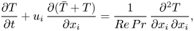 \begin{gather} \frac{\partial{T}}{\partial{t}}+u_{i}\,\frac{\partial{(\bar{T}+T)}}{\partial{x_{i}}}=\frac{1}{Re\,Pr}\,\frac{\partial^2{T}}{\partial{x_{i}}\,\partial{x_{i}}}, \end{gather}
where  $Re = U_bD/\nu$ is the (initial) Reynolds number, $Pr = \nu /\kappa$ is the Prandtl number, $Fr = U_b/(ND)$ is the Froude number, and $\bar {T}$ is the imposed background temperature. Stable stratification is imposed through $\partial {\bar {T}}/{\partial {t}}=0$, $\partial {\bar {T}}/{\partial {z}}= {\rm const.}$ and $\partial ^2{\bar {T}}/{\partial {z}^2}=0$. From here on, all variables are non-dimensional unless noted otherwise.
2.2. Initial conditions
The initial velocity field is decomposed into a mean velocity field  $\langle {u}\rangle$ and a fluctuating field $u'$. The mean field is given by
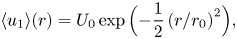 \begin{equation} \langle u_{1} \rangle(r)=U_{0}\exp\Big({-\frac{1}{2}\left({r}/{r_0}\right)^2}\Big), \end{equation}
where  $U_{0}$ here is the initial centreline velocity deficit, $r=\sqrt {x_{2}^2+x_{3}^2}$ is the radial distance from the wake centre, and $r_0$ is the initial wake radius. Here, $U_0 = 0.11$ and $r_0 = 1/2$, following Dommermuth et al. (Reference Dommermuth, Rottman, Innis and Novikov2002) and Brucker & Sarkar (Reference Brucker and Sarkar2010). The fluctuating field is generated as follows. First, a random field is generated from a uniform distribution between 0 and 1. Different realizations at given $Re$ and $Fr$ differ in these randomly generated initial fluctuation fields. Second, the field is made divergence-free and digitally filtered to match the energy spectrum
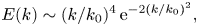 \begin{equation} E(k) \sim (k/k_0)^4\,{\rm e}^{{-}2(k/k_0)^2}, \end{equation}
where  $k_0 = 4$ (de Stadler et al. Reference de Stadler, Sarkar and Brucker2010). The initial turbulence intensity is denoted as $\alpha$ and is set to $0.055$. Third, the fluctuations are damped exponentially away from the centreline according to the damping function
 \begin{equation} g(r)=\alpha\Big(1+\frac{r}{r_0}\Big)^2\exp\Big(-\frac{1}{2}(r/r_0)^2\Big). \end{equation}
Fourth, we hold the mean field and allow the fluctuations to evolve until the cross-stream velocity fluctuation correlation is  $0.15 < \langle {u_{1}'u_{r}'} \rangle /K < 0.25$, where $K$ is the TKE, $u_1'$ is the root mean square of streamwise velocity fluctuation, and $u_r'$ is the root mean square of radial velocity fluctuation, $u_r'=\sqrt {u_2'^2+u_3'^2}$. This period lasts for approximately $t=7$. During the initial period, the gravitational force ( $1/Fr^2$) is turned off for $0< t<6$ and increases from 0 to the correct value in $6< t<8$ according to the ramping function
 \begin{equation} g(t)=g_{0}\tanh(t-t_{i}/t_{ramp}), \end{equation}
where  $t_{i}=6$ and $t_{ramp}=2$. The purpose of gravitational ramping is to compensate for the lack of temperature perturbation in the initial field. The set-up described here is based on the rationale presented in Brucker & Sarkar (Reference Brucker and Sarkar2007). For more detailed information on the initial condition, we refer the reader to Bevilaqua & Lykoudis (Reference Bevilaqua and Lykoudis1978), Uberoi & Freymuth (Reference Uberoi and Freymuth1970), Dommermuth et al. (Reference Dommermuth, Rottman, Innis and Novikov2002) and Brucker & Sarkar (Reference Brucker and Sarkar2010). According to Meunier & Spedding (Reference Meunier and Spedding2004) and Redford, Lund & Coleman (Reference Redford, Lund and Coleman2015), among others, the initialization should affect only the NW, and the wake should be universal further downstream.
2.3. Further details
Sponge layers are added at the vertical and transverse boundaries of the computational domain to absorb internal gravity waves, following the approach by Brucker & Sarkar (Reference Brucker and Sarkar2010). The size of the sponge layers is  $1$. Within the sponge layer, the velocity and temperature are damped using a Rayleigh damping function,
 \begin{equation} -\!\phi(x_i) [U_{i}(x_{i},t)-U_{i,\infty}], \quad -\phi(x_i) \left[ T(x_{i},t)-T_{\infty}\right], \end{equation}
which are added to the right-hand side of the momentum equations and the temperature transport equation, respectively. Here,  $U_{i,\infty }$ is the free stream velocity, and $T_{\infty }$ is the background temperature.
The grid used in the simulation is uniform in each of the three Cartesian directions, but the grid spacing varies in different directions. The resolution is chosen such that  $\Delta x/\eta < 4$ and $\Delta y/\eta, \Delta z/\eta < 2$, where $\eta$ represents the Kolmogorov scale and is taken as the minimum value of $\eta (x_2, x_3, t)$. The computational domain has size $60D$ in the streamwise direction, and the transverse and vertical sizes are chosen such that the boundaries are sufficiently far from the wake, following the guidelines of Diamessis et al. (Reference Diamessis, Spedding and Domaradzki2011). Further details of the grid resolution and domain dimensions can be found in table 4.
DNS details. The superscripts  $1, 2, 3$ denote the different stages of a case, and $t$ is the physical time simulated. ‘No. ens.’ is the number of ensembles computed.

The DNS are run until they reach the viscous regime, which is characterized by  $Re_{h}\,Fr_{h}^2<1$. This requires a long simulation time. To save computational resources, the domain is re-gridded during the simulation according to the method proposed by Gourlay et al. (Reference Gourlay, Arendt, Fritts and Werne2001), Redford, Castro & Coleman (Reference Redford, Castro and Coleman2012) and Redford et al. (Reference Redford, Lund and Coleman2015). The re-gridding is performed once or twice for each case. Specifically, the domain is re-gridded one time at $t = 110$ for the cases R20F02 and R20F10, two times at $t = 110$ and $t = 570$ for the case R20F50, and two times at $t = 68$ and $t = 265$ for the case R50F50. This leads to two or three stages for one case. This re-gridding process should have little to no influence on the wake according to Brucker & Sarkar (Reference Brucker and Sarkar2010).
The DNS are performed using the in-house finite-volume solver AFiD. The code utilizes second-order-accurate spatial discretization with a staggered grid and a low-storage third-order Runge–Kutta method for temporal discretization. Further details of the code can be found in Van Der Poel et al. (Reference Van Der Poel, Ostilla-Mónico, Donners and Verzicco2015), Ostilla-Mónico et al. (Reference Ostilla-Mónico, Yang, Van Der Poel, Lohse and Verzicco2015) and Kim & Moin (Reference Kim and Moin1985). The code has been used for stratified flows in Jain et al. (Reference Jain, Pham, Huang, Sarkar, Yang and Kunz2022), Yang et al. (Reference Yang, Van Der Poel, Ostilla-Mónico, Sun, Verzicco, Grossmann and Lohse2015, Reference Yang, Chen, Verzicco and Lohse2020), Du, Zhang & Yang (Reference Du, Zhang and Yang2021), Bin et al. (Reference Bin, Yang, Yang, Ni and Shi2022) and Li & Yang (Reference Li and Yang2021), among others. Here, a single R20F02 or R20F10 case requires approximately 2000 CPU hours; a single R20F50 realization requires 3000 CPU hours due to the increased simulation time; and a single R50F50 realization requires approximately 9000 CPU hours.
Finally, it is worth noting that the computational efficiency of computing multiple ensembles in a typically sized domain is superior to using an extremely long domain in the streamwise direction for our code. This is due to better parallelization and the convergence rate of the pressure Poisson equation. First, parallelization is generally more efficient for many small calculations than for a single large calculation for our code. Second, the convergence rate of the pressure Poisson equation depends on the mode with the longest wavelength. A long computational domain leads to a long wavelength mode, whose convergence rate is slow.
3. Results
3.1. Definitions
We define
 \begin{equation} {u_i}={\langle{u_i}\rangle} + u_i', \end{equation}
where  $u_i$ is the instantaneous velocity in the $i$th Cartesian direction, $\left \langle {\cdot }\right \rangle$ denotes streamwise and ensemble averaging, and $u_i'$ is the fluctuation. The width and height of the wake are denoted as
 \begin{equation} L_{H}, \quad L_{V}, \quad L_{Hk}, \quad L_{Vk} \quad {\rm and} \quad R_{i}, \end{equation}
where  $L_H$ and $L_V$ are the distances from the centre of the wake to where the velocity deficit is half of its centreline value in the horizontal and vertical directions, $L_{Hk}$ and $L_{Vk}$ are the distances from the centre of the wake to where the TKE is half of its centreline value, and $R_{i}$ are given by
 \begin{equation} R_i^2= A\frac{\displaystyle\int_C (x_i-x_i^c)^2{\langle{u_1}\rangle}^2 \,{\rm d}C}{{\displaystyle\int_C {\langle{u_1}\rangle}^2 \,{\rm d}C}}, \quad x_i^c = \frac{\displaystyle\int_C x_i{\langle{u_1}\rangle}^2 \,{\rm d}C}{{\displaystyle\int_C {\langle{u_1}\rangle}^2 \,{\rm d}C}}, \end{equation}
where  $i=2, 3$, $x_i^C$ is the centre location of the wake, integration is in the entire vertical transverse plane, and $A=2$ is a constant (de Stadler et al. Reference de Stadler, Sarkar and Brucker2010).
3.2. Benefits of ensemble averaging
We compare the results from one and many realizations to illustrate the benefit of ensemble averaging. For illustration purposes, the discussion here will focus on case R20F02.
Figure 6 shows the contours of mean velocity deficit at  $Nt=4$ (figures 6a,e), $Nt=30$ (figures 6b,f), $Nt=110$ (figures 6c,g) and $Nt=400$ (figures 6d,h) in the vertical transverse plane in case R20F02. The wake is in the NW regime at $Nt=4$, in the NEQ regime at $Nt=30$, and in the Q2D regime at $Nt=110$ and
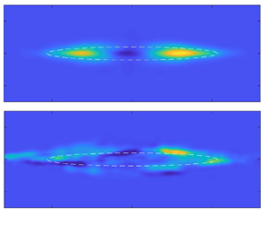
  $400$. The results obtained from one hundred samples are shown in figures 6(a–d), and the results obtained from one realization are shown in figures 6(e–h). We see that the results in figures 6(a,e) are similar, and thus the results from one sample and one hundred samples are similar in the NW regime. The difference between the two becomes evident in the late wake. The results from one hundred samples exhibit symmetry with respect to $y=0$ and have the maximum velocity deficit located at the centre of the wake. In contrast, the results from one realization do not show such symmetry and have the maximum velocity deficit shifted away from the centre; see figures 6(f–h). This lack of symmetry and deviation from the expected behaviour suggest that results obtained from one realization are not statistically converged. A lack of statistical convergence partly explains the scattering of the centreline velocity deficit data in table 1.
Contours of the velocity deficit in the vertical transverse plane in case R20F02. (a–d) Results obtained from one hundred samples, and (e–h) results obtained from one sample, for (a,e)  $Nt=4$, (b,f) $Nt=30$, (c,g) $Nt=110$, (d,h) $Nt=400$. For presentation purposes, we show only part of the domain. The white dashed lines indicate the core of the wakes, and they extend $2L_{Hk}$ and $2L_{Vk}$ in the $y$ and $z$ directions. The $+$ symbols indicate the wake centre defined in (3.3). The red circle symbols indicate the geometric centre of the wake, which is at $y=0$, $z=0$. Black lines indicate the contour lines of $1/4U_0$. The wake forms non-self-similar, diamond-shaped profiles in the late wake ( $Nt=110, 400$).

Figure 7 shows the contours of the TKE in case R20F02 at  $Nt=4$ (figures 7a,e,i), $Nt=30$ (figures 7b,f,j), $Nt=110$ (figures 7c,g,k) and $Nt=400$ (figures 7d,h,l). The results from one hundred samples are shown in figures 7(a–d), and the results from two independent realizations are shown in figures 7(e–h) and 7(i–l), respectively. The TKE is a second-order statistic, therefore obtaining statistically converged TKE is more challenging than obtaining statistically converged mean velocity deficit. While there was no apparent difference in the mean velocity deficit obtained from one and one hundred realizations in the NW regime, here we see a difference between one and one hundred ensembles as early as the NW regime. Insufficient averaging in the one-sample case leads to irregular variations across the vertical transverse plane, as seen in figures 7(e–h). In contrast, the results from one hundred samples, shown in figures 7(a–d), are regular and symmetric with respect to $y=0$. Specifically, the one-hundred-ensemble results display a single plateau at the centre of the wake, while the results from one realization show two-peak behaviour, particularly noticeable in figure 7(l). This discrepancy suggests that the two-peak behaviour reported in some realizations and in Brucker & Sarkar (Reference Brucker and Sarkar2010) is a result of insufficient averaging.
Contours of the TKE in the vertical transverse plane at (a,e,i)  $Nt=4$, (b,f,j) $Nt=30$, (c,g,k) $Nt=110$, and (d,h,l) $Nt=400$, in case R20F02. The dashed lines are contour lines. (a–d) One hundred ensembles. (e–h) Results from one realization. (i–l) Results from another realization.

Although it is not the focus of this study, higher-order statistics such as the terms in the TKE transport equation benefit more from ensemble averaging than low-order statistics such as the velocity deficit. Furthermore, the contours of the production term in the TKE transport equation are shown in figure 8. Comparing the results from one realization (figures 8e–h) with the results from one hundred realizations (figures 8a–d), it can be observed that ensemble averaging among one hundred realizations reveals structures of the production term that are not discernible from the result of a single realization. Specifically, the production term peaks towards the transverse boundary of the wake, and attains its minimum at the centre of the wake at  $Nt=30$, 110 and 400, as shown in figures 8(b–d).
Same as figure 6 but for the production term in the TKE transport equation: (a,e)  $Nt=4$, (b,f) $Nt=30$, (c,g) $Nt=110$, (d,h) $Nt=400$.

Figures 9(a–c) show the time evolution of the centreline velocity deficit, the wake width  $R_2$, and the wake height $R_3$, in case R10F02. The results from one realization may be anywhere between the blue and red lines in the figures, incurring significant uncertainties for the centreline velocity deficit and the width of the wake. Specifically, the uncertainty in the centreline velocity deficit and the wake width is as large as 100 % in the late wake. The results in figure 9 also help to explain the scattering of the data in tables 1 and 3.
Evolution of (a) the centreline velocity deficit, (b) the wake width and (c) the wake height, in case R10F02. Here, SSB10 denotes the results in de Stadler et al. (Reference de Stadler, Sarkar and Brucker2010), MAX and MIN are the maximum and minimum among the one hundred realizations, and AVG denotes results obtained from one hundred samples. Error bars in (a) and (b) characterize  ${+}100\,\%$ error about the min value, and the error bar in (c) characterizes ${+}15\,\%$ error with respect to the min value; $R_2$ and $R_3$ are defined in (3.3).

The findings in this subsection prompt re-evaluation of how computational resources are utilized in DNS of stratified wake flows. Currently, the prevailing approach in the literature is to allocate all available resources to a single calculation at the highest practically attainable Reynolds number (Diamessis et al. Reference Diamessis, Spedding and Domaradzki2011; de Bruyn Kops & Riley Reference de Bruyn Kops and Riley2019; Zhou & Diamessis Reference Zhou and Diamessis2019). The rationale is that data at high Reynolds numbers will help to clarify the Reynolds number scalings of flow statistics. Nonetheless, we can gain meaningful insights only if the convergence error in the results is smaller than the change induced by varying the Reynolds number. This might not be the case when there is only one realization. Therefore, it might be worthwhile to allocate resources to increase the number of statistical samples. Doing so will likely lead to more reliable data for further analysis. In this section, we will revisit the scaling behaviours of statistics including the centreline velocity deficit, the height and width of the wake, and terms in the TKE budget equation, with the goal of extracting more accurate scaling estimates.
3.3. The convergence error and the number of realizations
The convergence error depends on the number of independent samples, which further depends on the domain size and the number of independent realizations. We have kept the domain size the same between different realizations, and here, we focus on the effect of the number of independent realizations (or statistical samples). The discussion here will focus on case R20F02, which, as we will see, is the most challenging case. The effects of the Froude number and the Reynolds number will be discussed towards the end of the subsection.
Transverse symmetry of the flow dictates that the transverse location of the wake centre  $\langle x_2^c\rangle$ must be 0, therefore $|x_2^c|/L_{Hk}$ provides a measure of the convergence error in
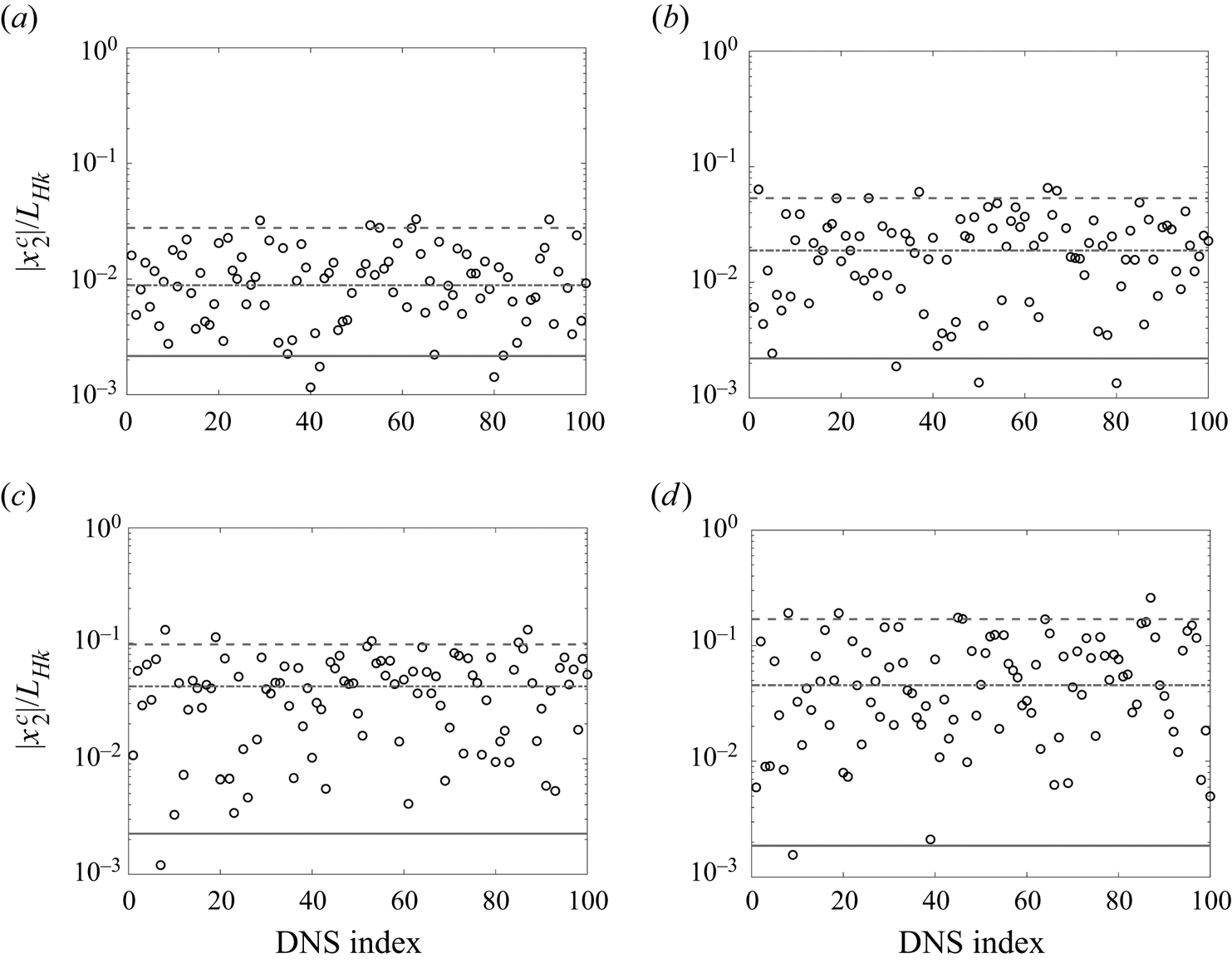
  $\langle x_2^c\rangle$. Figures 10(a–d) present $|x_2^c|/L_{Hk}$ for all one hundred realizations for case R20F02 at $Nt=4$, $30$,
$30$,  $110$ and $400$, respectively. The dashed lines and dash-dotted lines in the figure indicate the 5 % and 50 % margins, representing the probabilities that data from one realization would incur errors above these lines. We see from figure 10 that there is a 5 % probability that data from one realization incur an error larger than 0.028, 0.053, 0.098 and 0.17 at $Nt=4$, 30, 110 and 400, respectively; and there is a 50 % probability that data from one realization incur an error larger than 0.0088, 0.019, 0.042 and 0.045 at these time instants, respectively. We see that data from one realization incurs large convergence errors. Furthermore, the convergence error increases as the wake evolves. The solid lines represent the ensemble average of one hundred samples. The error is between 0.002 and 0.003 for the four time instants investigated here. Although there has not been much discussion on an acceptable level of convergence error for DNS of temporally evolving wakes in stratified environments, some discussion is available on the acceptable level of error for DNS of channel flow (Oliver et al. Reference Oliver, Malaya, Ulerich and Moser2014; Yang et al. Reference Yang, Hong, Lee and Huang2021; Chen et al. Reference Chen, Zhu, Shi and Yang2023). There, a 1 % error in the mean velocity profile with respect to the bulk velocity is considered acceptable. Applying the same standard to the current study and limiting the discussion to the convergence error only, we can conclude that one hundred realizations lead to statistically converged $x_2^c$ statistics.
Plots of  $|x_2^c|/L_{Hk}$ for all one hundred realizations for case R20F02 at (a) $Nt=4$, (b) $Nt=30$, (c) $Nt=110$, (d) $Nt=400$. The dashed line indicates the 5 % margin, the dash-dotted line indicates the 50 % margin, and the solid line indicates the ensemble average.
We discuss the number of realizations needed to obtain converged  $\langle x_2^c\rangle$. First and foremost, any finite number of statistical samples gives only an estimate of the true $\langle x_2^c\rangle$. The estimator itself is a random variable with mean being the true value of $\langle x_2^c\rangle$ (0 in this case), and standard deviation inversely proportional to the square root of the number of samples, i.e. $\sigma \sim 1/\sqrt {n}$. If there is a $p\%$ probability that the error is above $e$ when there are $N$ samples, then one needs $N (e/e')^2$ samples to claim that there is a $p\%$ probability that the error is above $e'$. From the data presented in figure 10, we can estimate that there would be a 50 % probability that the error is above 0.01 if we take averages among 1, 4, 17 and 20 samples at $Nt=4$, 30, 110 and 400, respectively; and there would be a 5 % probability that the error is above 0.01 if we take averages among 8, 28, 95 and 289 samples at these four time instants. We see that more samples are needed to get statistically converged data in the late wake than in the early wake. This is likely because of the large-scale structures in the late wake that lead to a reduction in the number of effective statistical samples in the domain.
Before we proceed further, we examine the unstratified wake results shown in figure 11. These results pertain to case R20F $\infty$ at the time instants $t=8$ and $800$, which correspond to $Nt=4$ and $400$ in case R20F02. The results exhibit similarities to those in figure 10. With 40 samples, the errors in the ensemble average are 0.21 % and 0.4 % at times $t=8$ and 800. There are 5 % and 50 % probabilities that data from one realization incur errors above 0.05 and 0.021 at $t=800$, and above 0.024 and 0.0096 at $t=8$. Comparing these numbers to those for R20F02, we can conclude that it is more straightforward to get converged statistics for an unstratified wake (for a given $t$).
$t$).
The centre location  $x_2^c/L_{Hk}$ for all realizations for case R20F $\infty$ at (a) $t=8$ and (b) $t=800$. The dashed line indicates the 5 % margin, the dash-dotted line indicates the 50 % margin, and the solid line indicates the ensemble average.

In addition to  $\langle x_2^c\rangle /L_{Hk}$, err defined below measures the spanwise asymmetry of the TKE, which also serves as a measure of the statistical convergence:
 \begin{equation}
{\textit{err}}=\frac{\displaystyle\int_{{-}2L_{Vk}}^{2L_{VK}}\displaystyle\int_{{-}2L_{Hk}}^{0}\left\langle
k\right\rangle {\rm d}y\,{\rm d}z -
\displaystyle\int_{{-}2L_{Vk}}^{2L_{VK}}\displaystyle\int_{0}^{2L_{Hk}}\left\langle
k\right\rangle {{\rm
d}y}}{{\displaystyle\int_{{-}2L_{Vk}}^{2L_{VK}}}\displaystyle\int_{{-}2L_{Hk}}^{2L_Hk}\left\langle
k\right\rangle{\rm d}y\,{\rm d}z}\times 100\,\%.
\end{equation}
\begin{equation}
{\textit{err}}=\frac{\displaystyle\int_{{-}2L_{Vk}}^{2L_{VK}}\displaystyle\int_{{-}2L_{Hk}}^{0}\left\langle
k\right\rangle {\rm d}y\,{\rm d}z -
\displaystyle\int_{{-}2L_{Vk}}^{2L_{VK}}\displaystyle\int_{0}^{2L_{Hk}}\left\langle
k\right\rangle {{\rm
d}y}}{{\displaystyle\int_{{-}2L_{Vk}}^{2L_{VK}}}\displaystyle\int_{{-}2L_{Hk}}^{2L_Hk}\left\langle
k\right\rangle{\rm d}y\,{\rm d}z}\times 100\,\%.
\end{equation} Figure 12 shows err as a function of the number of samples for case R20F02 at  $Nt=4$, 30, 110 and 400. For any given number of samples, e.g. $n$, we randomly draw $n$ samples from all available realizations five times. As a result, for any given $n$, there are five data points. The trends are similar at the four time instants. The error decreases rapidly as the number of statistical samples increases from 1 to 20, and does not decrease significantly beyond 40–60 statistical samples. For the four time instants investigated here, the error is approximately 1 %–2 % when there are approximately 40–60 samples. Again, there is not a lot of discussion about the acceptable level of error in the context of DNS of stratified wake flows, but there is discussion in the context of DNS of channel flow. There, an approximately 2 %–3 % error in TKE is considered acceptable. We see that approximately 40–60 samples bring us to that regime, with the late wake requiring more realizations.
Plots of err in case R20F02 at (a)  $Nt=4$, (b) $Nt=30$, (c) $Nt=110$, (d) $Nt=400$. For any given number of samples $n$, err is computed five times by randomly drawing $n$ samples from the available realizations. The solid line is at $err=2\,\%$.
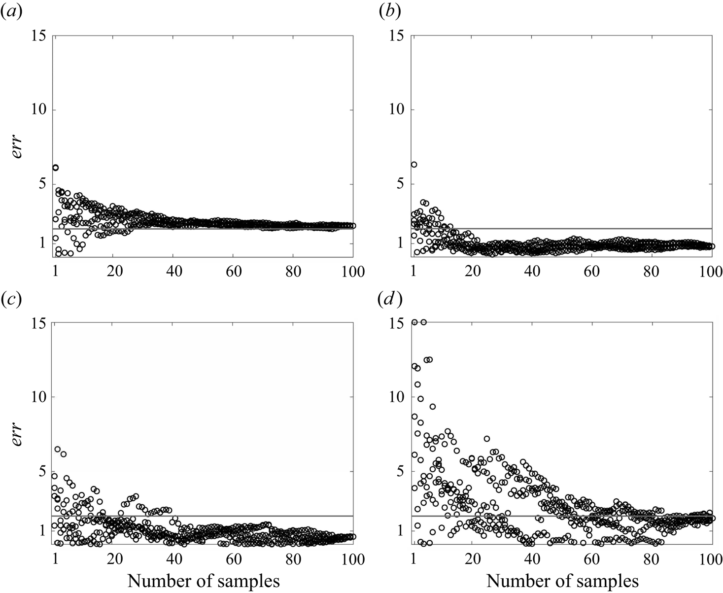
Finally, figure 13 shows the results for cases R20F10, R20F50, R50F50 and R20F $\infty$ at time $t=800$ (corresponding to $Nt=400$ for case R20F02). We observe the following. First, the ensemble average in these cases reduces the convergence error to 2 % at $t=800$. Second, stratification has a notable effect on the result. Comparing figures 12(d) and 13(a–d), we see that for a given number of statistical samples, case R20F02 incurs a significantly larger convergence error than the other stratified cases (R20F10, R20F50 and R50F50), and the other stratified cases incur larger convergence errors than the unstratified case. Third, comparing figures 13(b,c), we see that there is no apparent Reynolds number effect from varying the Reynolds number by a factor 2.5.
Plots of err at  $t=800$ in cases (a) R20F10, (b) R20F50, (c) R50F50, (d) R20F $\infty$. For any given number of samples $n$, err is computed five times by randomly drawing $n$ samples from the available realizations. The solid line is at $err=2\,\%$.

3.4. Centreline velocity deficit
Figure 14(a) presents the time evolution of the centreline velocity deficit  $U_0$, the horizontal and vertical velocity fluctuations $u_h'$ and $w'$, and the square root of the TKE for cases R20F50 and R50F50. We see no apparent Reynolds number effect at the given range of the Reynolds numbers. In both cases, the centreline velocity decays as $Nt^{-2/3}$ in the NW regime up to $Nt\approx 1$; the decay rate decreases between $Nt=1$ and $Nt=50$ in the NEQ regime, and increases beyond $Nt=50$ in the Q2D regime. Contrary to the existing literature, we see no clear evidence of a $-0.25$ scaling or a $-0.76$ scaling. In fact, it is hard to find any power-law scaling. The decay rate changes continuously without staying constant for an extended period of time. This becomes more clear from figure 14(b), where we show the premultiplied centreline velocity deficit, i.e. $t^{0.25} U_0$. If there is a region within which the centreline velocity deficit follows $U_0\sim (Nt)^{-0.25}$, then we should observe a plateau in figure 14(b). However, no such a region can be identified. The $t^{0.76}$ compensated centreline velocity deficit is shown in the Appendix, and no plateau can be observed there either.
(a) Evolution of centreline velocity deficit  $U_0$, horizontal and vertical velocity fluctuations $u_h'$ and $w'$, and root mean square of the TKE in cases R20F50 and R50F50. The solid lines represent the R50F50 case, and the dashed lines represent the R20F50 case. (b) Premultiplied centreline velocity deficit.
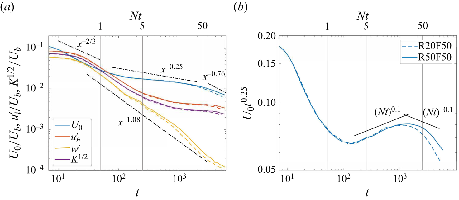
Figure 15(a) shows the results for case R20F10, and figure 15(b) shows the results for cases R10F02 and R20F02. Similar to previous cases, no significant Reynolds number effect is evident in these figures. Due to the strong buoyancy effect, a distinct NW regime is barely observable in the two F02 cases. If one defines the beginning of the NEQ regime to be the time instant at which the  $U_0$ decay rate begins to decrease, then it is clear from figures 14(a) and 15(a,b) that the onset of the NEQ regime depends on the Froude number. Figures 15(c,d) show the premultiplied centreline velocity deficit. Once again, we do not see a plateau. We also examined the $U_0t^{2/3}$ compensated scalings in the Appendix, and no plateaus are identified there either.
(a,b) Evolution of centreline velocity deficit  $U_0$, horizontal and vertical velocity fluctuations $u_h'$ and $w'$, and root mean square of the TKE in cases (a) R20F10, (b) R20F02 and R10F02. We use dashed lines for R20F02 and solid lines for R10F02. (c,d) Premultiplied centreline velocity deficit.

Finally, figure 16 shows the power-law exponent  $b\equiv {\rm d}\log (U_0)/{\rm d}\log (t)$, or the decay rate of the centreline velocity deficit, as a function of the non-dimensional time $Nt$ for all four cases. The plots are shown in both log and linear scales. The estimates in Meunier et al. (Reference Meunier, Diamessis and Spedding2006) are included for comparison. We notice a discontinuity in the estimate at $Nt\approx 2$, prior to which is the NW regime and $b=-2/3$ (Tennekes & Lumley Reference Tennekes and Lumley1972; Meunier et al. Reference Meunier, Diamessis and Spedding2006). We make the following observations. First, the initial period of the wake evolution is affected by the initialization. The gravitational ramping lasts until $t=8$, which corresponds to $Nt=4$, $0.8$ and $0.16$ for $Fr=2$, $10$ and $50$, respectively. In a plot whose $x$ axis is $Nt$, initialization will appear to have a more significant impact on wakes with lower Froude numbers. Second, the computed power-law exponents show a reasonable level of collapse. The value of the power-law exponent is approximately $-2/3$ for $Nt\lesssim 1$, decreases to approximately $-0.1$ between $Nt\approx 5$ and $Nt\approx 10$, then gradually increases. Third, the estimate in Meunier et al. (Reference Meunier, Diamessis and Spedding2006) provides a reasonable approximation of the data. According to the estimate, the decay rate attains its minimum 0.1 at $Nt=2$. Although the data suggest that the decay rate attains its minimum between $Nt\approx 5$ and $Nt\approx 10$, the value is indeed approximately 0.1. The estimate also captures the gradual increase of the decay rate in the stratified turbulence regime – although there are discrepancies, particularly when the flow is strongly stratified. Finally, the anticipated Q2D regime asymptotics, where $b$ approaches $-0.76$, are not observed in our data.
Power-law exponent  $b={\rm d}\log (U_0)/{\rm d}\log (t)$ as a function of $Nt$. Solid lines represent the theoretical predictions in Meunier et al. (Reference Meunier, Diamessis and Spedding2006) and the symbols are our DNS results: (a) linear-log scale; (b) linear-linear scale.

3.5. Velocity fluctuations
The evolution of the horizontal and vertical velocity fluctuations  $u_h'$, $w'$ and the square root of the TKE $K^{1/2}$ in R20F50 and R50F50 is shown in figure 14(a). From the plot, we observe that the results are not affected significantly by the Reynolds number, at least within the range of Reynolds numbers investigated in this study. Both the vertical and horizontal velocity fluctuations follow approximately a power-law decay with an exponent close to $-1.08$ in the NW regime between $Nt=0.8$ and $Nt=4$. This is consistent with the ${-1}$ scaling reported in Chongsiripinyo & Sarkar (Reference Chongsiripinyo and Sarkar2020) and is in agreement with the $t^{-1.08}$ scaling reported in Brucker & Sarkar (Reference Brucker and Sarkar2010). The vertical velocity fluctuation continues to decay as $Nt^{-1.08}$ in the NEQ and Q2D regimes until the end of the simulation. On the other hand, the decay rate of the horizontal velocity fluctuations decreases as the flow enters the NEQ regime, and remains almost constant between $Nt=20$ and $Nt=80$. Due to this disparate decay rate between $u_h'$ and $w'$ in the NEQ and Q2D regimes, $u_h'$ becomes increasingly larger than $w'$ as the wake evolves. Consequently, the TKE is $K\approx u_h'/\sqrt {2}$.
Figure 15(a) shows the time evolution of  $u_h'$, $w'$ and $K'$ in case R20F10, and figure 15(b) shows the corresponding results for cases R10F02 and R20F02. In the two F02 cases, a clear NW regime can barely be observed as the flow quickly enters the NEQ regime after the initialization period. In the NEQ and Q2D regimes, the decay rates of the horizontal velocity fluctuations and the square root of the TKE continue to increase. It is worth noting that the undulations in $w'$ observed in the two F02 cases are the result of rapid exchange between TKE and available potential energy. Interestingly, these undulations are limited to $w'$ in our DNS, while others have reported undulations in $U_0$ as well (Pal et al. Reference Pal, Sarkar, Posa and Balaras2017; Chongsiripinyo & Sarkar Reference Chongsiripinyo and Sarkar2020). The vertical velocity fluctuation $w'$ follows a power law at these cases shortly after the calculation begins and all the way into the viscous regime. A least squares fit of the data gives power-law exponents $-1.19$ and $-1.29$ at the F10 and F02 cases, which are slightly different from the exponent in the F50 case.
Furthermore, by comparing the decay of  $w'$ at different Froude numbers, it becomes evident that the exponent increases as $Fr$ decreases. An empirical fit of decay of $w'$ as a function of $Fr$ gives $w'=x^{-1.33+0.065\ln (Fr)}$. Nevertheless, further study is needed to clarify the exact effects of the Froude number and consolidate this empirical scaling estimate.
3.6. Length scale statistics
Figure 17 shows the time evolution of the wake width and height, denoted as  $L_H$, $L_V$, $L_{Hk}$ and $L_{Vk}$. As before, $L_H$ and $L_V$ represent the distance from the wake centre to where the velocity deficit is half of its centreline value, while $L_{Hk}$ and $L_{Vk}$ measure the distance from the wake centre to where the TKE is half of its centreline value. First, we observe that the Reynolds number has a negligible effect on the data. From figure 17(a), we can see that the wake width $L_H$ grows as $(Nt)^{1/3}$ in the NW regime; its growth rate decreases at $Nt\approx 5$ and increases shortly after that. The $1/3$ power law provides a good working approximation of $L_H$ throughout the NW, NEQ and Q2D regimes. From figure 17(b), we see that the wake height $L_V$, also grows as $(Nt)^{1/3}$ in the NW regime; it then decreases in the NEQ regime, and reaches its minimum at $Nt\approx 50$ before it begins to increase again. The decrease of $L_V$ in the NEQ regime was also found in Davidson (Reference Davidson2010) and Chongsiripinyo & Sarkar (Reference Chongsiripinyo and Sarkar2020), where it was attributed to buoyancy effects. The estimates in Meunier et al. (Reference Meunier, Diamessis and Spedding2006) are included in figures 17(a,b) for comparison. Despite some quantitative differences, the estimates from Meunier et al. (Reference Meunier, Diamessis and Spedding2006) capture the overall trend quite well. For instance, the estimate in Meunier et al. (Reference Meunier, Diamessis and Spedding2006) captures accurately the decrease and subsequent increase in the $L_H$ decay rate in the NEQ regime. Additionally, it also captures the suppression of the vertical length scale in the stratified flow regime. Finally, figures 17(c,d) depict $L_{Hk}$ and $L_{Vk}$. The two length scales behave similarly to $L_H$ and $L_V$, with $L_{Hk}$ growing faster than $L_H$, and $L_{Vk}$ decreasing more rapidly in the NEQ regime following a $-0.4$ power law (Chongsiripinyo & Sarkar Reference Chongsiripinyo and Sarkar2020).
Wake width and height as functions of the non-dimensional time  $Nt$: (a) $L_H$, (b) $L_V$, (c) $L_{Hk}$, (d) $L_{Vk}$. The solid lines represent estimates in Meunier et al. (Reference Meunier, Diamessis and Spedding2006). Again, normalization is by the diameter of the wake-generating body.

Before we conclude this subsection, we comment on the interplay between  $U_0$, $L_H$ and $L_V$. If the wake profile is such that $U=U_0(x)\,f(\kern0.7pt y/L_H,z/L_V)$, where $f$ is generic function, then the momentum conservation would imply that $U_0L_HL_V={\rm const.}$ (Meunier et al. Reference Meunier, Diamessis and Spedding2006). Figure 18(a) illustrates the evolution of $U_0L_VL_H$, which shows that this statistic is approximately constant after an initial transient period. We denote this constant as $C_m$. In figures 18(b,c), we compare $U_0$ with $C_m/(L_HL_V)$ and $C_m/[L_VC_H(Nt)^{1/3}]$, where $L_H\approx C_H(Nt)^{1/3}$. Here, $C_H$ is obtained from fitting the wake width data. We observe that the three quantities agree well. With the decay of $L_H$ contributing to a $-1/3$ power-law decay throughout, the results in figures 18(b,c) suggest that the decrease in the $U_0$ decay rate in the NEQ regime is mainly due to the decreasing $L_V$, while the increase in the $U_0$ decay rate in the Q2D regime is a result of the increasing $L_V$.
Plots of (a)  $U_0L_vL_H$, (b) $C_m/(L_V L_H)$ and (c) $C_m/[L_VC_H(Nt)^{-1/3}]$, as functions of time. The plots (b,c) are shifted vertically by an arbitrary distance so that they collapse at $Nt=10$. Solid lines represent the estimated $U_0$, whereas the dashed line denotes $U_0$ in the DNS.

3.7. TKE budget
We devote this section to the TKE budget. The TKE transport equation reads
 \begin{equation} \frac{\partial k}{\partial t}={-}\mathcal{C}+\mathcal{P}-\mathcal{D}+\mathcal{B}-\mathcal{T}. \end{equation}
Here,  $\mathcal{C}$ is the convection term
 \begin{equation} \mathcal{C} \equiv \langle{u_i}\rangle\,\frac{\partial{k}}{x_i}, \end{equation} $\mathcal{P}$ is the production term
 \begin{equation} \mathcal{P} \equiv{-}\langle{u_i'u_j'}\rangle\frac{\partial{u_i}}{\partial{x_j}}, \end{equation} $\mathcal{D}$ is the dissipation term
 \begin{equation} \mathcal{D} \equiv \frac{2}{Re_0}\,\langle{s_{ij}'s_{ij}'}\rangle, \end{equation}
where
 \begin{equation} s_{ij}'=\frac{1}{2}\left(\frac{\partial{u_i}'}{\partial{x_j}}+\frac{\partial{u_j}'}{\partial{x_i}}\right), \end{equation} $\mathcal{B}$ is the buoyancy flux term
 \begin{equation} \mathcal{B} \equiv{-}\frac{1}{Fr^2}\,\langle{u_3'T'}\rangle, \end{equation}
and  $\mathcal{T}$ is the transport/diffusion term
 \begin{equation} \mathcal{T} \equiv \frac{\partial{\langle{u_i'p'}}\rangle}{\partial{x_i}}+\frac{1}{2}\,\frac{\partial{\langle{u_i'u_j'u_j'}}\rangle}{\partial{x_i}}-\frac{2}{Re_0}\,\frac{\partial\langle u_j's_{ij}'\rangle}{\partial{x_i}}. \end{equation}
 Pal & Sarkar (Reference Pal and Sarkar2015), Redford et al. (Reference Redford, Lund and Coleman2015) and Chongsiripinyo & Sarkar (Reference Chongsiripinyo and Sarkar2020), among others, have reported the time evolution of the transverse and vertical integrated (integrated in both directions) terms in the TKE equation. Following these authors, we first report the transverse and vertical integrated terms. The integration is over  $-2L_{Hk}< y<2L_{Hk}$ and $-2L_{Vk}< y<2L_{Vk}$, representing the core of the wake. Also, since the flow is not affected significantly by the Reynolds number in the investigated range, the analysis here will focus on a high-Froude-number case R50F50 and a low-Froude-number case R20F02.
Figures 19(a–d) show the evolution of the budget terms for case R50F50; the values of the budget terms vary vastly from one time to another, so we have plotted separately  $0.2< Nt<1$, $1< Nt<3$, $3< Nt<15$ and $15< Nt<110$, respectively. The production term and the dissipation terms are the dominant terms for $Nt\lesssim 0.5$. Dissipation is by far the most dominant term between $Nt\approx 1$ and $Nt\approx 10$. From $Nt\approx 15$ until the end of the simulation, the production, transport and dissipation terms are the most significant terms. We note that buoyancy is never significant. It is also worth noting that our results align closely with the budget reported in Brucker & Sarkar (Reference Brucker and Sarkar2010), suggesting that even one statistical sample is sufficient for transverse and vertically integrated budget terms. Figure 20 shows the transverse and vertically integrated budget terms for case R20F02. Unlike in case R50F50, the buoyancy term is a dominant term from the early stage until $Nt\approx 30$, which is consistent with the findings in Chongsiripinyo & Sarkar (Reference Chongsiripinyo and Sarkar2020). Additionally, the buoyancy term exhibits rapid sign changes during the early stage, alternating between acting as a sink and a source, which manifests the exchange between the available potential energy and TKE (Redford et al. Reference Redford, Lund and Coleman2015; Chongsiripinyo & Sarkar Reference Chongsiripinyo and Sarkar2020). This behaviour explains the observed undulations in $K^{1/2}$ and $w'$ as depicted in figure 15(b). In the late wake, the dissipation and production terms emerge as dominant, which is similar to R50F50. Finally, the transport term is comparable to the production term between $Nt\approx 15$ and $Nt\approx 35$, but becomes negligibly small beyond $Nt\approx 100$.
The volume integrated TKE budget terms in case R50F50,  $X=\int _V \mathcal {X}\,{\rm d}V$, where $\mathcal {X}$ represents the terms in the budget equation (3.5). Note that we did not divide the volume, following Brucker & Sarkar (Reference Brucker and Sarkar2010). Plots of the budget terms as a function of $Nt$ (a) from 0.2 to 1, (b) from 1 to 3, (c) from 3 to 15, (d) from 15 to 110. Here, P, C, B, T and D represent the production, convective, buoyancy, transport and dissipation terms.
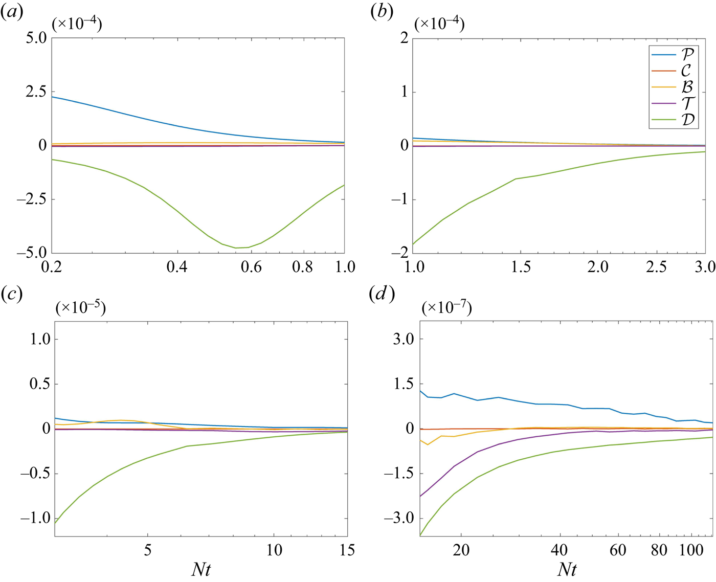
Same as figure 19 but for R20F02. Plots of the budget terms as a function of  $Nt$ (a) from 4 to 15, (b) from 15 to 50, (c) from 50 to 180, (d) from 180 to 400.

By integrating in both the transverse and vertical directions, one obtains statistics that are less susceptible to convergence errors, but information pertaining to the transverse and vertical distributions is lost. In this study, we have obtained many statistical samples. They allow us to integrate in one direction yet still get converged data.
Figure 21 shows the transverse integrated budget terms as well as the vertically integrated budget terms in R50F50 at three time instants,  $Nt=2$, 30 and 110, corresponding to the NW, NEQ and Q2D regimes, respectively. The transverse integrated terms are shown in figures 21(a,c,e) as functions of the vertical coordinate $z$. The vertically integrated terms are shown in figures 21(b,d,f) as functions of the transverse coordinate $y$. We first examine the terms in the NW regime. The dissipation term is the dominant term, and it has similar distributions in the vertical and the transverse directions – in the sense that one could not tell if the quantity is vertically integrated or transverse integrated from the plots themselves. The other terms are small. Next, we examine the terms in the NEQ regime. The production, dissipation and transport terms are the dominant terms. The wake is anisotropic, with significant differences between the transverse and vertically integrated terms. The transverse integrated production and transport terms have one peak at the wake centre, whereas the vertically integrated production and transport terms have two peaks at $y/L_{Hk}\approx \pm 0.6$. Additionally, the transverse integrated dissipation term shows double peaks at $z/L_{Vk}\approx \pm 0.6$, while the vertically integrated dissipation term has a single peak at the wake centre. The destruction terms, i.e. the dissipation and transport terms, are largely balanced by the production term. This explains the reduced decay rate of $K^{1/2}$ in the NEQ regime. Finally, we examine the terms in the Q2D regime: they are not qualitatively different from their counterparts in the NEQ regime. The dominant terms remain production, dissipation and transport. However, the balance between these terms changes. The production term decreases faster than the destruction terms, leading to a faster decay of $K^{1/2}$ in the Q2D regime. An interesting observation is that the vertically integrated production term becomes negative at the wake centre, indicating that the mean flow extracts energy from turbulence in that region.
The terms in the TKE budget equation in case R50F50: (a,b)  $Nt=2$, (c,d) $Nt=30$, and (e,f) $Nt=110$. (a,c,e) Integrated in the transverse direction, $X=\int _y \mathcal {X}\,{{\rm d} y}$. (b,d,f) Integrated in the vertical direction, $X=\int _z \mathcal {X}\,{\rm d}z$. Here, P, C, B, T and D denote the production, convective, buoyancy, transport and dissipation terms. Considering the symmetry with respect to the centreline, we show only results from the wake centre.
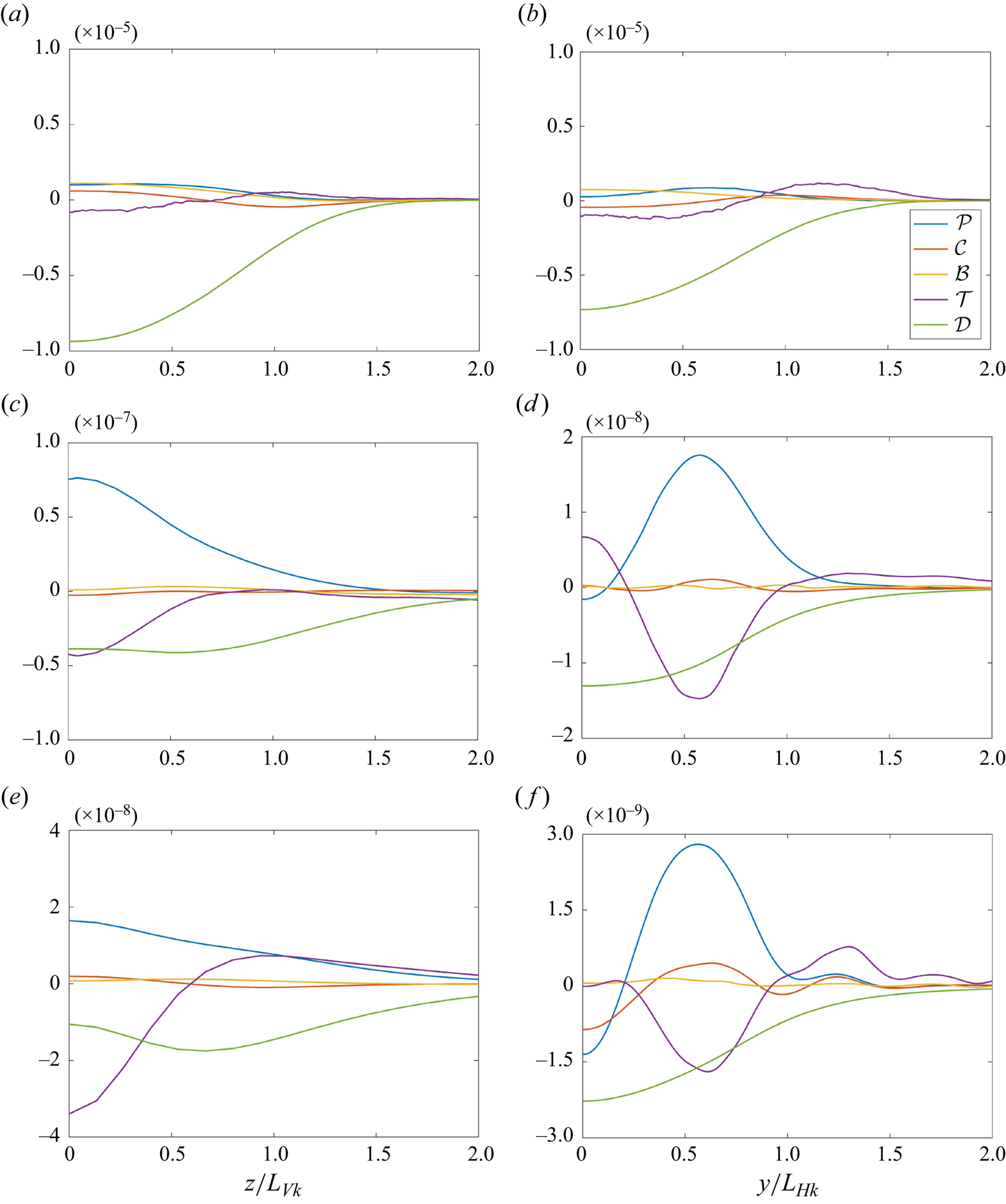
Figure 22 presents the transverse integrated budget terms and the vertically integrated terms in case R20F02. The buoyancy term is the dominant term in the NW regime. From figure 20, we know that the term flips sign in the early wake. While the term is positive at  $Nt=4$, it is negative at $Nt=5.5$ (not shown). The production, dissipation and transport terms are the dominant terms in the lake wake, similar to R50F50. However, unlike R50F50, the destruction terms in R20F02 are noticeably larger than the generation terms. This leads to a fast decaying $K^{1/2}$, as is evident in figure 15(b). It is interesting that the transport terms take energy from the wake centre and put it near the edge of the wake in the late wake, as shown in figures 21(d,f) and 22(d,f).
The terms in the TKE budget equation in case R20F02: (a,b)  $Nt=4$, (c,d) $Nt=30$, and (e,f) $Nt=110$. (a,c,e) Integrated in the transverse direction. (b,d,f) Integrated in the vertical direction. Legend is the same as in figure 21.

4. Concluding remarks
We report DNS results of temporally evolving wake at Reynolds numbers from 10 000 to 50 000, and Froude numbers from 2 to 50. Instead of computing statistics from one realization, we take ensemble averages among 80–100 realizations. To assess the statistical convergence of our data, two statistical objects are considered: the transverse location of the wake centre, denoted as  $x_2^c$, and the transverse asymmetry in the TKE, denoted as err. Both should be 0 when there are sufficiently many statistical samples. The analysis shows high convergence error when data are taken from one realization. The convergence error quickly decreases as the number of realizations/samples increases. The benefit, however, diminishes beyond 20 and 60 realizations before and after entering Q2D regimes, respectively.
The data allow us to assess the previously established scaling laws and establish new scaling estimates. First, the velocity deficit, denoted as  $U_0$, does not seem to follow any power-law scaling in the late wake. The decay rate, defined as $-{\rm d}\log (U_0)/{\rm d}\log (t)$, attains its minimum 0.1 at a time between $Nt=5$ and $Nt=10$, and increases continuously as the wake evolves. No power-law scalings are found in $L_H$ or $L_V$ either, but $L_H\sim (Nt)^{1/3}$ proves to be a good working approximation of the wake width. Furthermore, while the wake is not self-similar, $U_0L_HL_V$ is approximately a constant after the initial transient period. It follows that $U_0\sim (Nt)^{-1/3}/L_V$. Hence we may conclude that the decrease in the $U_0$ decay rate in the NEQ regime is a result of the decrease in the wake's vertical size, and that the increase in the $U_0$ decay rate in the Q2D regime is a consequence of the increase in the wake's vertical size. Finally, the power-law decay of the vertical velocity fluctuation is verified, but there is no power-law decay in the horizontal velocity fluctuation.
In addition to low-order statistics, we report the transverse integrated budget terms, the vertically integrated budget terms, and the budget terms integrated in both cross-sectional directions. The behaviours of these terms as functions of the vertical and transverse coordinates have not received much attention due to the high number of ensembles needed to get converged statistics. Our data suggest that there are two peaks in the vertically integrated production and transport terms at  $y=\pm 0.6 L_{Hk}$, and one peak at the wake centre when the terms are transverse integrated. It is interesting that the transverse integrated production term is negative at the wake centre, suggesting energy transfer from turbulence to the mean flow.
Finally, we add a caveat. Although the results do not seem to be affected significantly by the Reynolds number, the Reynolds numbers investigated here (i.e. 10 000 to 50 000) are quite limited. The Reynolds number of a wake behind an underwater vehicle can be as high as  $O(10^9)$ (Li, Yang & Kunz Reference Li, Yang and Kunz2022). Work by Meunier et al. (Reference Meunier, Diamessis and Spedding2006) and Brucker & Sarkar (Reference Brucker and Sarkar2010) suggests that the NEQ regime extends as the Reynolds number increases. A lack of power-law decay of the centreline velocity deficit in the NEQ regime can be a result of the limited Reynolds number, which needs to be investigated further.
Funding
This work was sponsored by the US Office of Naval Research under contract N000142012315, with Dr P. Chang as Technical Monitor.
Declaration of interests
The authors report no conflict of interest.
Appendix. Additional results
In this section, we present additional results.
We present the rescaled/premultiplied centreline velocity deficit and wake width and height in figures 23 and 24. The centreline velocity deficit is premultiplied with  $Fr^{2/3}$ in figure 23(a).
Rescaled centreline velocity deficit.

Rescaled evolution of wake width and height as functions of the non-dimensional time  $Nt$: (a) $L_H$, (b) $L_V$, (c) $L_{Hk}$, (d) $L_{Vk}$.

Compared to figure 3, premultiplying  $Fr^{2/3}$ helps to collapse data, but there are still notable differences among the F02, F10 and F50 cases. Premultiplying $Fr^{0.54}$ yields good data collapse. Here, $Fr^{0.54}$ is entirely empirical. Figure 24 shows the rescaled wake width and height. The horizontal length scales $L_H$ and $L_{Hk}$ show good collapse after premultiplying $Fr^{-1/3}$. The vertical length scales $L_V$ and $L_{Vk}$, on the other hand, do not collapse after premultiplying $Fr^{-1/3}$. This is similar to the results reported by Spedding (Reference Spedding2002). However, as shown in figure 25, the data still show compromising collapse after rescaling with $Fr^{-0.6}$ as suggested by Spedding (Reference Spedding2002).
Rescaled evolution of  $L_V$ with $Fr^{-0.6}$.
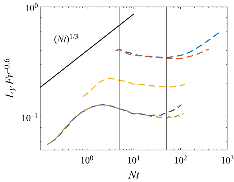
Figure 26(a) shows the premultiplied  $L_H$. We see that $L_H(Nt)^{-1/3}$ is approximately a constant. Figure 26(b) shows the $Nt^{0.76}$ premultiplied centreline velocity deficit. We do not see any plateau in the plot.
Premultiplied evolution of (a)  $L_H$, (b) $U_0$.


 Open access