





1. Introduction
The flow past a sphere is one of the most extensively studied flows, both experimentally and numerically (Tiwari et al. Reference Tiwari, Pal, Bale, Minocha, Patwardhan, Nandakumar and Joshi2020a
), because the sphere is the most symmetric body with aspect ratio close to $1$
. Nevertheless, the scenario of the transition to turbulence past a sphere is still an open question.
$1$
. Nevertheless, the scenario of the transition to turbulence past a sphere is still an open question.
The first steps of the transition are well known (Tiwari et al. Reference Tiwari, Pal, Bale, Minocha, Patwardhan, Nandakumar and Joshi2020b
). The flow exhibits fore–aft symmetry at very low Reynolds numbers ( ${\textit{Re}}$
), which is lost when the Reynolds number increases: a stationary recirculation bubble appears at
${\textit{Re}}$
), which is lost when the Reynolds number increases: a stationary recirculation bubble appears at ${\textit{Re}} \sim 20$
. Above
${\textit{Re}} \sim 20$
. Above ${\textit{Re}} \sim 210$
, the rotational symmetry is lost, but the flow remains planar symmetric and stationary. The main feature of the flow above this threshold is a pair of counter-rotating streamwise vortices, observed even at distances much larger than the length of the recirculation zone. Above
${\textit{Re}} \sim 210$
, the rotational symmetry is lost, but the flow remains planar symmetric and stationary. The main feature of the flow above this threshold is a pair of counter-rotating streamwise vortices, observed even at distances much larger than the length of the recirculation zone. Above ${\textit{Re}}_1 \sim 270$
, the counter-rotating streamwise vortices begin to oscillate with Strouhal number
${\textit{Re}}_1 \sim 270$
, the counter-rotating streamwise vortices begin to oscillate with Strouhal number ${\textit{St}}_1$
, i.e. this regime corresponds to periodic vortex shedding. The two counter-rotating streamwise vortices merge periodically to form out-of-plane structures, the so-called ‘hairpins’.
${\textit{St}}_1$
, i.e. this regime corresponds to periodic vortex shedding. The two counter-rotating streamwise vortices merge periodically to form out-of-plane structures, the so-called ‘hairpins’.
The next step is the onset of a new frequency that is lower than the first one and associated with Strouhal number ${\textit{St}}_2$
. Several articles reported this low frequency in the velocity field or in the forces on the sphere, obtained using numerical or experimental approaches; see table 1.
${\textit{St}}_2$
. Several articles reported this low frequency in the velocity field or in the forces on the sphere, obtained using numerical or experimental approaches; see table 1.
However, this low frequency has not been studied systematically experimentally. The characteristics of this low frequency remain poorly understood. The value of the threshold Reynolds number ${\textit{Re}}_2$
for this low frequency depends on the study, with most of the reported values ranging between
${\textit{Re}}_2$
for this low frequency depends on the study, with most of the reported values ranging between $320$
and
$320$
and $390$
(see table 1). This may be partly due to differences in the choice of the velocity used in the Reynolds number, in particular for experiments where the flow far from the sphere cannot be perfectly homogeneous due to solid boundaries. The value of the Strouhal number
$390$
(see table 1). This may be partly due to differences in the choice of the velocity used in the Reynolds number, in particular for experiments where the flow far from the sphere cannot be perfectly homogeneous due to solid boundaries. The value of the Strouhal number ${\textit{St}}_2$
is also widely scattered; see table 1. In most of the articles, the ratio
${\textit{St}}_2$
is also widely scattered; see table 1. In most of the articles, the ratio ${\textit{St}}_2/{\textit{St}}_1$
ranges between
${\textit{St}}_2/{\textit{St}}_1$
ranges between $0.25$
and
$0.25$
and $0.3$
, but some very low frequencies were reported in the numerical works of Kalro & Tezduyar (Reference Kalro and Tezduyar1998) and Lu et al. (Reference Lu, Lin, Lin and Chang2024). The dispersion of the data of the literature is displayed in figure 1. As consequence of this dispersion, small variations of the extrapoled value of the frequency at the origin produce a decrease of
$0.3$
, but some very low frequencies were reported in the numerical works of Kalro & Tezduyar (Reference Kalro and Tezduyar1998) and Lu et al. (Reference Lu, Lin, Lin and Chang2024). The dispersion of the data of the literature is displayed in figure 1. As consequence of this dispersion, small variations of the extrapoled value of the frequency at the origin produce a decrease of ${\textit{St}}_2$
with the Reynolds number as in the numerical work of Mittal & Najjar (Reference Mittal and Najjar1999), or an increase as in the numerical work of Tiwari et al. (Reference Tiwari, Bale, Patwardhan, Nandakumar and Joshi2019) (see table 1). In a recent work, Schuh Frantz et al. (Reference Schuh Frantz, Mimeau, Salihoglu, Loiseau and Robinet2025) investigated numerically the nature of the bifurcation using linear stability analysis, which they report to be a secondary Hopf bifurcation.
${\textit{St}}_2$
with the Reynolds number as in the numerical work of Mittal & Najjar (Reference Mittal and Najjar1999), or an increase as in the numerical work of Tiwari et al. (Reference Tiwari, Bale, Patwardhan, Nandakumar and Joshi2019) (see table 1). In a recent work, Schuh Frantz et al. (Reference Schuh Frantz, Mimeau, Salihoglu, Loiseau and Robinet2025) investigated numerically the nature of the bifurcation using linear stability analysis, which they report to be a secondary Hopf bifurcation.
Threshold Reynolds numbers ${\textit{Re}}_1$
and
${\textit{Re}}_1$
and ${\textit{Re}}_2$
past a sphere, reported in the literature. Values of the Strouhal numbers
${\textit{Re}}_2$
past a sphere, reported in the literature. Values of the Strouhal numbers $\mathit{St}_1$
,
$\mathit{St}_1$
, $\mathit{St}_2$
and
$\mathit{St}_2$
and $\mathit{St}_2/\mathit{St}_1$
past a sphere, for Reynolds number
$\mathit{St}_2/\mathit{St}_1$
past a sphere, for Reynolds number ${\textit{Re}}$
. ‘Num.’ indicates numerical, and ‘Exp.’ indicates experimental. The precise definition of the Reynolds number depends on the article (in particular due to boundary layers in experiments in channels).
${\textit{Re}}$
. ‘Num.’ indicates numerical, and ‘Exp.’ indicates experimental. The precise definition of the Reynolds number depends on the article (in particular due to boundary layers in experiments in channels).

A low frequency was observed in the flow past other three-dimensional bodies: rotating sphere (Lorite-Díez & Jiménez-González Reference Lorite-Díez and Jiménez-González2020), cube (Meng et al. Reference Meng, An, Cheng and Kimiaei2021), disk (Berger, Scholz & Schumm Reference Berger, Scholz and Schumm1990; Auguste et al. Reference Auguste, Fabre and Magnaudet2010; Yang et al. Reference Yang, Liu, Wu, Liu and Zhang2015; Gao et al. Reference Gao, Tao, Tian and Yang2018), incline prolate spheroid (Wang et al. Reference Wang, Yang, Andersson, Zhu, Liu, Wang and Lu2021), rectangular prism (Chiarini & Boujo Reference Chiarini and Boujo2025), blunt-based axisymmetric body (Bohorquez et al. Reference Bohorquez, Sanmiguel-Rojas, Sevilla, Jiménez-González and Martínez-Bazán2011; Bury & Jardin Reference Bury and Jardin2012; Rigas et al. Reference Rigas, Oxlade, Morgans and Morrison2014; Pavia et al. Reference Pavia, Varney, Passmore and Almond2019; Tran & Chen Reference Tran and Chen2020; Zhang & Peet Reference Zhang and Peet2023) and short cylinder (Yang, Feng & Zhang Reference Yang, Feng and Zhang2022).
Ratio $\mathit{St}_2/\mathit{St}_1$
as a function of the Reynolds number. Data are from the literature; see table 1.
$\mathit{St}_2/\mathit{St}_1$
as a function of the Reynolds number. Data are from the literature; see table 1.

The spatial features and the physical mechanisms associated with the low frequency past a sphere remain unclear, as stated by Tiwari et al. (Reference Tiwari, Pal, Bale, Minocha, Patwardhan, Nandakumar and Joshi2020b
): ‘the physics associated with it and the range of ${\textit{Re}}$
for which they exist are yet unknown’.
${\textit{Re}}$
for which they exist are yet unknown’.
A first mechanism that is often mentioned is the rotation of the plane of emission of the vortices. The rotation of the separation point azimuthally around the rear part of the sphere is mentioned by Tomboulides & Orszag (Reference Tomboulides and Orszag2000), and this assertion is based on the visualisation of the three-dimensional vorticity in numerical simulations. In the work of Lee (Reference Lee2000), it is noted that ‘individual vortex shedding occurs from different locations behind the sphere’. In the review article by Kiya, Ishikawa & Sakamoto (Reference Kiya, Ishikawa and Sakamoto2001), it is mentioned that the ‘low-frequency component is interpreted as the central frequency of the irregular rotation of the hairpin vortices’. Brücker (Reference Brücker2001) describes the ‘typical slight random variations of the orientation of the vortices’. The ‘significant cycle-to-cycle variations in the orientation of the vortex’ are noted in Mittal, Wilson & Najjar (Reference Mittal, Wilson and Najjar2002). The ‘irregular transversal rotation’ is shown experimentally in Chrust, Goujon-Durand & Wesfreid (Reference Chrust, Goujon-Durand and Wesfreid2013) by flow visualisation using a fluorescent dye illuminated by a laser sheet in a plane perpendicular to the streamwise direction. An oscillation in the shedding direction from left to right is also mentioned in Sakamoto & Haniu (Reference Sakamoto and Haniu1990), based on visualisation of the flow using dye.
Another feature mentioned in the literature is that the low frequency is associated with a ‘pumping mode’ of the recirculation bubble. For example, several snapshots show that the wake undergoes expansion and contraction in Tiwari et al. (Reference Tiwari, Bale, Patwardhan, Nandakumar and Joshi2019), but no quantitative analysis was provided. Similarly, the low frequency past a blunt-based axisymmetric body at ${\textit{Re}}=5000$
was shown to be located close to the object, by computing the dynamic mode decomposition and proper orthogonal decomposition modes from numerical simulations (Zhang & Peet Reference Zhang and Peet2023). Using coherence spectra from a hot-wire anemometer, Berger et al. (Reference Berger, Scholz and Schumm1990) showed that the low frequency past a disk at much higher Reynolds number
${\textit{Re}}=5000$
was shown to be located close to the object, by computing the dynamic mode decomposition and proper orthogonal decomposition modes from numerical simulations (Zhang & Peet Reference Zhang and Peet2023). Using coherence spectra from a hot-wire anemometer, Berger et al. (Reference Berger, Scholz and Schumm1990) showed that the low frequency past a disk at much higher Reynolds number ${\textit{Re}}=2.1 \times 10^5$
is dominant inside the recirculation bubble.
${\textit{Re}}=2.1 \times 10^5$
is dominant inside the recirculation bubble.
Experimental set-up.

Like the first frequency, the low frequency was observed at higher Reynolds numbers: at ${\textit{Re}}= 3700$
in the numerical work of Rodriguez et al. (Reference Rodriguez, Borell, Lehmhuhl, Segarra, Carlos and Oliva2011), and at
${\textit{Re}}= 3700$
in the numerical work of Rodriguez et al. (Reference Rodriguez, Borell, Lehmhuhl, Segarra, Carlos and Oliva2011), and at ${\textit{Re}}= 2 \times 10^4$
in the numerical work of Robertson et al. (Reference Robertson, Choudhury, Bhushan and Walters2015). This underlines the relevance of this low frequency in the dynamics of the flow past a sphere, even far from the bifurcation at
${\textit{Re}}= 2 \times 10^4$
in the numerical work of Robertson et al. (Reference Robertson, Choudhury, Bhushan and Walters2015). This underlines the relevance of this low frequency in the dynamics of the flow past a sphere, even far from the bifurcation at ${\textit{Re}}_2$
.
${\textit{Re}}_2$
.
In the present paper, we study experimentally the bifurcations associated with the main frequency $f_1$
and with the low frequency
$f_1$
and with the low frequency $f_2$
. We investigate the associated Strouhal numbers, and the corresponding amplitudes, as a function of the Reynolds number and position. The experimental set-up are presented in § 2, and snapshots of the vorticity field are shown in § 3. The variation of the main and low frequencies with the Reynolds number, and the interpretation of the other peaks as combinations of these two frequencies, are discussed in § 4, and the nature of the bifurcation is discussed in § 5. Section 6 focuses on the components of the streamwise vorticity field at
$f_2$
. We investigate the associated Strouhal numbers, and the corresponding amplitudes, as a function of the Reynolds number and position. The experimental set-up are presented in § 2, and snapshots of the vorticity field are shown in § 3. The variation of the main and low frequencies with the Reynolds number, and the interpretation of the other peaks as combinations of these two frequencies, are discussed in § 4, and the nature of the bifurcation is discussed in § 5. Section 6 focuses on the components of the streamwise vorticity field at $f_1$
and
$f_1$
and $f_2$
, and the spatial variation as a function of the distance downstream from the sphere.
$f_2$
, and the spatial variation as a function of the distance downstream from the sphere.
2. Experimental set-up
The experiments were performed in a transparent closed water channel with cross-section $S={0.1 \times 0.1}\ {{\textrm{m}}^2}$
and turbulence intensity below 4
$S={0.1 \times 0.1}\ {{\textrm{m}}^2}$
and turbulence intensity below 4 $\,\%$
(see figure 2). This water channel was already used in previous studies investigating three-dimensional bluff body wakes, including spheres and cubes, as described e.g. in Gumowski et al. (Reference Gumowski, Miedzik, Goujon-Durand, Jenffer and Wesfreid2008), Klotz et al. (Reference Klotz, Goujon-Durand, Rokicki and Wesfreid2014) and Skarysz et al. (Reference Skarysz, Rokicki, Goujon-Durand and Wesfreid2018). In this paper, we report the velocity field behind a plastic sphere of diameter
$\,\%$
(see figure 2). This water channel was already used in previous studies investigating three-dimensional bluff body wakes, including spheres and cubes, as described e.g. in Gumowski et al. (Reference Gumowski, Miedzik, Goujon-Durand, Jenffer and Wesfreid2008), Klotz et al. (Reference Klotz, Goujon-Durand, Rokicki and Wesfreid2014) and Skarysz et al. (Reference Skarysz, Rokicki, Goujon-Durand and Wesfreid2018). In this paper, we report the velocity field behind a plastic sphere of diameter $D={14}\,\textrm{mm}$
. The sphere is mounted using a metal rod of diameter
$D={14}\,\textrm{mm}$
. The sphere is mounted using a metal rod of diameter ${1.9}\,\textrm{mm}$
. This rod is in the plane
${1.9}\,\textrm{mm}$
. This rod is in the plane $y=0$
, and consists of a vertical part fixed at the top of the channel and a horizontal part of length
$y=0$
, and consists of a vertical part fixed at the top of the channel and a horizontal part of length ${135}\,\textrm{mm}$
. The sphere is fixed at the end of this horizontal part.
${135}\,\textrm{mm}$
. The sphere is fixed at the end of this horizontal part.
The temperature of water is measured using a Hanna Instruments Checktemp digital thermometer, of accuracy $\pm {0.3}\,^\circ {\textrm {C}}$
. The kinematic viscosity of water
$\pm {0.3}\,^\circ {\textrm {C}}$
. The kinematic viscosity of water $\nu$
is deduced from the temperature (see https://www.engineeringtoolbox.com/water-dynamic-kinematic-viscosity-d_596.html).
$\nu$
is deduced from the temperature (see https://www.engineeringtoolbox.com/water-dynamic-kinematic-viscosity-d_596.html).
The flow rate $Q$
is measured at least three times for each operating condition, using a bucket and a stopwatch. The measurement repeatability is approximately
$Q$
is measured at least three times for each operating condition, using a bucket and a stopwatch. The measurement repeatability is approximately $1\,\%$
. The mean velocity
$1\,\%$
. The mean velocity $U$
is defined using the flow rate and the surface
$U$
is defined using the flow rate and the surface $U=Q/S$
, as in the previous publications using this channel (Gumowski et al. Reference Gumowski, Miedzik, Goujon-Durand, Jenffer and Wesfreid2008). Due to boundary layers, the velocity at the centre of the channel upstream of the sphere is slightly larger than
$U=Q/S$
, as in the previous publications using this channel (Gumowski et al. Reference Gumowski, Miedzik, Goujon-Durand, Jenffer and Wesfreid2008). Due to boundary layers, the velocity at the centre of the channel upstream of the sphere is slightly larger than $U$
. The Reynolds number
$U$
. The Reynolds number ${\textit{Re}}$
is defined using the velocity
${\textit{Re}}$
is defined using the velocity $U$
and the diameter of the sphere:
$U$
and the diameter of the sphere: ${\textit{Re}}=UD/\nu$
. In this paper,
${\textit{Re}}=UD/\nu$
. In this paper, $U$
ranges between
$U$
ranges between ${16\times 10^{-3}}\ {{\textrm{m}\ \text{s}}^{-1}}$
and
${16\times 10^{-3}}\ {{\textrm{m}\ \text{s}}^{-1}}$
and ${43\times 10^{-3}}\ {{\textrm{m}\ \text{s}}^{-1}}$
, and
${43\times 10^{-3}}\ {{\textrm{m}\ \text{s}}^{-1}}$
, and ${\textit{Re}}$
ranges between
${\textit{Re}}$
ranges between $250$
and
$250$
and $550$
. The temperature of water varies between
$550$
. The temperature of water varies between ${13.7}\,^\circ{\textrm{C}}$
and
${13.7}\,^\circ{\textrm{C}}$
and ${21.0}\,^\circ {\textrm {C}}$
, thus the kinematic viscosity varies between
${21.0}\,^\circ {\textrm {C}}$
, thus the kinematic viscosity varies between ${1.18 \times 10^{-6}}\ {\textrm{m}^2 \,\textrm{s}^{-1}}$
and
${1.18 \times 10^{-6}}\ {\textrm{m}^2 \,\textrm{s}^{-1}}$
and ${0.98 \times 10^{-6}}\ {\textrm{m}^2 \,\textrm{s}^{-1}}$
. The uncertainty on the Reynolds number is mostly due to the uncertainty on
${0.98 \times 10^{-6}}\ {\textrm{m}^2 \,\textrm{s}^{-1}}$
. The uncertainty on the Reynolds number is mostly due to the uncertainty on $U$
and the temperature, and is approximately
$U$
and the temperature, and is approximately $1\,\%$
.
$1\,\%$
.
The transverse velocity field is measured in six different $yz$
planes, with the distance
$yz$
planes, with the distance $X$
to the centre of the sphere ranging from
$X$
to the centre of the sphere ranging from $X=0.8D$
to
$X=0.8D$
to $X=9D$
(where
$X=9D$
(where $(0,0,0)$
is the centre of the sphere). The laser sheet is generated by a Quantel Big Sky double pulsed Nd:YAG laser with
$(0,0,0)$
is the centre of the sphere). The laser sheet is generated by a Quantel Big Sky double pulsed Nd:YAG laser with ${532}\,\textrm{nm}$
emission and
${532}\,\textrm{nm}$
emission and ${250}\,\textrm{mJ}$
per pulse at
${250}\,\textrm{mJ}$
per pulse at ${10}\,\textrm{Hz}$
. We use a ‘thick’ laser sheet of width approximately
${10}\,\textrm{Hz}$
. We use a ‘thick’ laser sheet of width approximately ${3}\,\textrm{mm}$
. This ensures that despite the quite large streamwise velocity (of order
${3}\,\textrm{mm}$
. This ensures that despite the quite large streamwise velocity (of order $U$
), the particles remain in the laser sheet during the acquisition of the image pair. We use LaVision HQ
$U$
), the particles remain in the laser sheet during the acquisition of the image pair. We use LaVision HQ ${20}\,{\unicode{x03BC}\textrm {m}}$
polyamide particles for the seeding. The laser pulse delay ranges from
${20}\,{\unicode{x03BC}\textrm {m}}$
polyamide particles for the seeding. The laser pulse delay ranges from $15$
ms to
$15$
ms to ${25}\,\textrm{ms}$
, with the higher value corresponding to the lower values of
${25}\,\textrm{ms}$
, with the higher value corresponding to the lower values of $U$
. This delay is small enough to have most of the particles in the sheet in the first image remain in the sheet in the second one
$U$
. This delay is small enough to have most of the particles in the sheet in the first image remain in the sheet in the second one
The images are acquired using an Imager Pro Plus 2M $12$
bits camera equipped either with a Nikon
$12$
bits camera equipped either with a Nikon ${50}\,\textrm{mm}$
or an
${50}\,\textrm{mm}$
or an ${85}\,\textrm{mm}$
objective and an aperture fixed at
${85}\,\textrm{mm}$
objective and an aperture fixed at $f/5.6$
.
$f/5.6$
.
The laser and the camera are synchronised using a PTU-X synchroniser. The resulting images were $ 1600\times 1200$
pixels. The calibration is performed for each plane by measuring the distance between the channel walls on the image, yielding a magnification factor ranging from
$ 1600\times 1200$
pixels. The calibration is performed for each plane by measuring the distance between the channel walls on the image, yielding a magnification factor ranging from $8.75$
to
$8.75$
to $9.76$
pixels mm−1.
$9.76$
pixels mm−1.
The acquisition time is ${420}\,\textrm{s}$
, corresponding to
${420}\,\textrm{s}$
, corresponding to $4200$
pairs of images and at least
$4200$
pairs of images and at least $30$
periods of the low frequency.
$30$
periods of the low frequency.
The velocity vectors are obtained from cross-correlation using Davis 10 from LaVision®. The interrogation window size for the initial pass is $256 \times 256$
, then three passes with interrogation windows of
$256 \times 256$
, then three passes with interrogation windows of $32\times 32$
pixels with overlap
$32\times 32$
pixels with overlap $50 \,\%$
are performed, resulting in a spatial grid of
$50 \,\%$
are performed, resulting in a spatial grid of $148 \times 98$
points.
$148 \times 98$
points.
The velocity fields are processed using Python programs to obtain the streamwise vorticity field (i.e. along the $x$
direction) by derivation. The periodograms of the variables are computed using the Python function scipy.signal.periodogram. The options are chosen to remove the offset of the signal before computing the periodogram, and to obtain the squared magnitude spectrum (and not the power spectral density), so that the amplitude of the peaks are independent of the duration of the signal. In the following, all variables without an explicit dimension are dimensionless, and are made dimensionless with
$x$
direction) by derivation. The periodograms of the variables are computed using the Python function scipy.signal.periodogram. The options are chosen to remove the offset of the signal before computing the periodogram, and to obtain the squared magnitude spectrum (and not the power spectral density), so that the amplitude of the peaks are independent of the duration of the signal. In the following, all variables without an explicit dimension are dimensionless, and are made dimensionless with $U$
and
$U$
and $D$
unless stated otherwise. For instance, the Strouhal number
$D$
unless stated otherwise. For instance, the Strouhal number $\mathit{St}$
is defined as
$\mathit{St}$
is defined as $\mathit{St}=fD/U$
, where
$\mathit{St}=fD/U$
, where $f$
is the frequency, and the streamwise vorticity is normalised by
$f$
is the frequency, and the streamwise vorticity is normalised by $U/D$
.
$U/D$
.
3. Vorticity fields
Snapshots of the streamwise vorticity field for ${\textit{Re}} = 322$
and
${\textit{Re}} = 322$
and $X=3$
. The vertical and horizontal lines are guides for the eye; the circle is the projection of the position of the sphere in the
$X=3$
. The vertical and horizontal lines are guides for the eye; the circle is the projection of the position of the sphere in the $yz$
plane.
$yz$
plane.

Snapshots of the vorticity field for ${\textit{Re}} = 409$
and
${\textit{Re}} = 409$
and $X=3$
. The vertical and horizontal lines are guides for the eye; the circle is the projection of the position of the sphere in the
$X=3$
. The vertical and horizontal lines are guides for the eye; the circle is the projection of the position of the sphere in the $yz$
plane.
$yz$
plane.

A series of snapshots of the streamwise vorticity field at $X=3$
and
$X=3$
and ${\textit{Re}} = 322$
(resp.
${\textit{Re}} = 322$
(resp. ${\textit{Re}} = 409$
) is shown in figure 3 (resp. figure 4). The duration is approximately two periods
${\textit{Re}} = 409$
) is shown in figure 3 (resp. figure 4). The duration is approximately two periods $T_1$
of the main frequency (with
$T_1$
of the main frequency (with $T_1=1/f_1$
). The vorticity field is periodic for
$T_1=1/f_1$
). The vorticity field is periodic for ${\textit{Re}} = 322$
(see figure 3): the vorticity field is very similar for two snapshots of the same column, which are separated by a time close to
${\textit{Re}} = 322$
(see figure 3): the vorticity field is very similar for two snapshots of the same column, which are separated by a time close to $T_1$
. The counter-rotating vortices are particularly visible at
$T_1$
. The counter-rotating vortices are particularly visible at $t=0.00T_1$
,
$t=0.00T_1$
, $t=0.21 T_1$
,
$t=0.21 T_1$
, $t=0.81 T_1$
and the corresponding times after one period. The value of the vorticity field of the counter-rotating vortices in the measurement plane changes with time. Moreover, the counter-rotating vortices move slightly in the
$t=0.81 T_1$
and the corresponding times after one period. The value of the vorticity field of the counter-rotating vortices in the measurement plane changes with time. Moreover, the counter-rotating vortices move slightly in the $y$
direction. At times
$y$
direction. At times $t=0.42 T_1$
,
$t=0.42 T_1$
, $t=0.60 T_1$
and the corresponding times after one period, the counter-rotating vortices are less visible: this corresponds to the times at which the head of the hairpins crosses the measurement plane. The vorticity in the plane of measurement is then small. Other small-amplitude vorticity structures can be seen above the two counter-rotating vortices. Similar steady structures are observed upstream of the sphere (data not shown): these are associated with the mounting rod. The corresponding velocity field is mainly a downward vertical velocity. The modulation of the streamwise vorticity due to the Bénard–von Kármán vortices emitted by the rod is negligible, and the sphere does not vibrate. At a higher Reynolds number, i.e.
$t=0.60 T_1$
and the corresponding times after one period, the counter-rotating vortices are less visible: this corresponds to the times at which the head of the hairpins crosses the measurement plane. The vorticity in the plane of measurement is then small. Other small-amplitude vorticity structures can be seen above the two counter-rotating vortices. Similar steady structures are observed upstream of the sphere (data not shown): these are associated with the mounting rod. The corresponding velocity field is mainly a downward vertical velocity. The modulation of the streamwise vorticity due to the Bénard–von Kármán vortices emitted by the rod is negligible, and the sphere does not vibrate. At a higher Reynolds number, i.e. ${\textit{Re}} = 409$
displayed in figure 4, the vorticity field is almost periodic with period
${\textit{Re}} = 409$
displayed in figure 4, the vorticity field is almost periodic with period $T_1$
. However, more differences can be seen for two velocity fields in the same column, i.e. after a time interval
$T_1$
. However, more differences can be seen for two velocity fields in the same column, i.e. after a time interval $T_1$
. These differences correspond to the presence of a low frequency, as shown in the following.
$T_1$
. These differences correspond to the presence of a low frequency, as shown in the following.
4. Frequencies
4.1. Barycentre
Variation of the position $(G_y,G_z)$
at
$(G_y,G_z)$
at $X=3$
of the barycentre of the absolute value of vorticity, over
$X=3$
of the barycentre of the absolute value of vorticity, over ${60}\,\textrm{s}$
.
${60}\,\textrm{s}$
.

The frequencies can be detected on many variables deduced from the velocity field. However, the relative amplitude of the different frequencies depends a lot on the chosen variable. We first present the barycentre $(G_y,G_z)$
of the absolute value of the streamwise vorticity field. This variable is approximately the ‘centre’ of the two main vortices when they are present, slightly shifted due to the vorticity structures above the sphere (due to the mounting rod). It provides a clear determination of the main and low frequencies. Another barycentre related to the momentum deficit was already used as a variable (Grandemange, Gohlke & Cadot Reference Grandemange, Gohlke and Cadot2014; Gentile et al. Reference Gentile, Schrijer, Van Oudheusden and Scarano2016; Yokota & Nonomura Reference Yokota and Nonomura2024), but to our knowledge, not the barycentre of the absolute value of the vorticity field.
$(G_y,G_z)$
of the absolute value of the streamwise vorticity field. This variable is approximately the ‘centre’ of the two main vortices when they are present, slightly shifted due to the vorticity structures above the sphere (due to the mounting rod). It provides a clear determination of the main and low frequencies. Another barycentre related to the momentum deficit was already used as a variable (Grandemange, Gohlke & Cadot Reference Grandemange, Gohlke and Cadot2014; Gentile et al. Reference Gentile, Schrijer, Van Oudheusden and Scarano2016; Yokota & Nonomura Reference Yokota and Nonomura2024), but to our knowledge, not the barycentre of the absolute value of the vorticity field.
Examples of trajectories of the barycentre for different Reynolds numbers are given in figure 5. The trajectory at ${\textit{Re}}=268$
is a point, widened by the noise due to this measurement method. This is consistent with the presence of a stationary pair of counter-rotating vortices. At
${\textit{Re}}=268$
is a point, widened by the noise due to this measurement method. This is consistent with the presence of a stationary pair of counter-rotating vortices. At ${\textit{Re}}=322$
, the trajectory is a cycle, consistent with a single frequency in the dynamics. This cycle proceeds clockwise. The amplitude of the displacement in the
${\textit{Re}}=322$
, the trajectory is a cycle, consistent with a single frequency in the dynamics. This cycle proceeds clockwise. The amplitude of the displacement in the $y$
direction, which corresponds to the motion of the counter-rotating vortices, is smaller than the motion in the
$y$
direction, which corresponds to the motion of the counter-rotating vortices, is smaller than the motion in the $z$
direction. The latter is influenced by the small steady vorticity structures above the two counter-rotating vortices. The displacement in the
$z$
direction. The latter is influenced by the small steady vorticity structures above the two counter-rotating vortices. The displacement in the $y$
direction is, however, larger than that in the
$y$
direction is, however, larger than that in the $z$
direction for planes at a greater distance from the sphere (data not shown). The trajectory at the highest Reynolds numbers
$z$
direction for planes at a greater distance from the sphere (data not shown). The trajectory at the highest Reynolds numbers ${\textit{Re}}=409$
and
${\textit{Re}}=409$
and ${\textit{Re}}=526$
is irregular. In the following, we discuss the frequencies involved in the dynamics for
${\textit{Re}}=526$
is irregular. In the following, we discuss the frequencies involved in the dynamics for ${\textit{Re}}=322$
and
${\textit{Re}}=322$
and ${\textit{Re}}=409$
.
${\textit{Re}}=409$
.
Plots for ${\textit{Re}}=322$
,
${\textit{Re}}=322$
, $X=3$
: (a) position
$X=3$
: (a) position $G_y$
along
$G_y$
along $y$
of the barycentre as a function of time (in pixels); (b) periodogram of
$y$
of the barycentre as a function of time (in pixels); (b) periodogram of $G_y$
. The main frequency is
$G_y$
. The main frequency is $f_1={0.262\pm 0.003}\,\textrm{Hz}$
.
$f_1={0.262\pm 0.003}\,\textrm{Hz}$
.

Plots for ${\textit{Re}}=409$
,
${\textit{Re}}=409$
, $X=3$
: (a) position
$X=3$
: (a) position $G_y$
along
$G_y$
along $y$
of the barycentre as a function of time; (b) periodogram of
$y$
of the barycentre as a function of time; (b) periodogram of $G_y$
. The symbols correspond to integer combinations of
$G_y$
. The symbols correspond to integer combinations of $f_1$
and
$f_1$
and $f_2$
, with some values indicated above the graph.
$f_2$
, with some values indicated above the graph.

Plots for ${\textit{Re}}=409$
,
${\textit{Re}}=409$
, $X=3$
: (a) position
$X=3$
: (a) position $G_z$
along
$G_z$
along $z$
of the barycentre as a function of time; (b) periodogram of
$z$
of the barycentre as a function of time; (b) periodogram of $G_z$
. The symbols correspond to integer combinations of
$G_z$
. The symbols correspond to integer combinations of $f_1$
and
$f_1$
and $f_2$
.
$f_2$
.

The position $G_y$
of the barycentre as a function of time, and the associated periodogram at
$G_y$
of the barycentre as a function of time, and the associated periodogram at ${\textit{Re}}=322$
, are shown in figure 6. The signal is very regular, and only the first harmonic
${\textit{Re}}=322$
, are shown in figure 6. The signal is very regular, and only the first harmonic $f_1$
, the second harmonic
$f_1$
, the second harmonic $2f_1$
and the third harmonic
$2f_1$
and the third harmonic $3f_1$
are observed in the periodogram (below
$3f_1$
are observed in the periodogram (below ${1}\,\textrm{Hz}$
). The squared magnitude, which will be used below, is defined as the amplitude of the peaks in the periodogram, where squared variables are displayed. The motion along
${1}\,\textrm{Hz}$
). The squared magnitude, which will be used below, is defined as the amplitude of the peaks in the periodogram, where squared variables are displayed. The motion along $y$
of the barycentre corresponds to the main motion of the counter-propagating vortices, i.e. hairpin shedding (see figure 1 of Bobinski, Goujon-Durand & Wesfreid Reference Bobinski, Goujon-Durand and Wesfreid2014), observed in the transverse plane
$y$
of the barycentre corresponds to the main motion of the counter-propagating vortices, i.e. hairpin shedding (see figure 1 of Bobinski, Goujon-Durand & Wesfreid Reference Bobinski, Goujon-Durand and Wesfreid2014), observed in the transverse plane $X=3$
.
$X=3$
.
The position $G_y$
of the barycentre as a function of time at a higher Reynolds number (
$G_y$
of the barycentre as a function of time at a higher Reynolds number ( ${\textit{Re}}=409$
) and the corresponding periodogram are shown in figure 7. The signal is less regular, and is no longer periodic. Many peaks are visible. The peak of largest magnitude is at
${\textit{Re}}=409$
) and the corresponding periodogram are shown in figure 7. The signal is less regular, and is no longer periodic. Many peaks are visible. The peak of largest magnitude is at $f_1$
, the second largest at
$f_1$
, the second largest at $f_1+f_2$
, the third at
$f_1+f_2$
, the third at $f_2$
. The peak at
$f_2$
. The peak at $f_1+f_2$
is consistent with the modulated aspect of the signal. Similar peaks were already observed by Mittal (Reference Mittal1999), Schouveiler & Provansal (Reference Schouveiler and Provansal2002) and Schuh Frantz et al. (Reference Schuh Frantz, Mimeau, Salihoglu, Loiseau and Robinet2025). The other peaks are integer combinations of the peaks at
$f_1+f_2$
is consistent with the modulated aspect of the signal. Similar peaks were already observed by Mittal (Reference Mittal1999), Schouveiler & Provansal (Reference Schouveiler and Provansal2002) and Schuh Frantz et al. (Reference Schuh Frantz, Mimeau, Salihoglu, Loiseau and Robinet2025). The other peaks are integer combinations of the peaks at $f_1$
and
$f_1$
and $f_2$
, consistent with the
$f_2$
, consistent with the $T^2$
torus dynamics described in Schuh Frantz et al. (Reference Schuh Frantz, Mimeau, Salihoglu, Loiseau and Robinet2025). The other coordinate of the barycentre, i.e.
$T^2$
torus dynamics described in Schuh Frantz et al. (Reference Schuh Frantz, Mimeau, Salihoglu, Loiseau and Robinet2025). The other coordinate of the barycentre, i.e. $G_z$
, and the corresponding periodogram are displayed in figure 8. In this figure, the peak with the largest amplitude is at
$G_z$
, and the corresponding periodogram are displayed in figure 8. In this figure, the peak with the largest amplitude is at $f_2$
, the second larger at
$f_2$
, the second larger at $f_1$
, and the third at
$f_1$
, and the third at $f_1-f_2$
. The relative amplitude of the peaks thus depends on the considered variable. We take advantage of this result to determine the main frequency
$f_1-f_2$
. The relative amplitude of the peaks thus depends on the considered variable. We take advantage of this result to determine the main frequency $f_1$
from the periodogram of
$f_1$
from the periodogram of $G_y$
(figure 7, for instance) and the value of
$G_y$
(figure 7, for instance) and the value of $f_2$
from the periodogram of
$f_2$
from the periodogram of $G_z$
(figure 8, for instance). The selected value of the frequency usually corresponds to the peak of largest amplitude. However, in a limited number of cases, the second-highest peak was selected to avoid any discontinuity in the curve.
$G_z$
(figure 8, for instance). The selected value of the frequency usually corresponds to the peak of largest amplitude. However, in a limited number of cases, the second-highest peak was selected to avoid any discontinuity in the curve.
4.2. Variation of the Strouhal number with the Reynolds number
Strouhal number corresponding to the first frequency $f_1$
, as a function of the Reynolds number. Inset: same data, plotting Roshko number as a function of Reynolds number, and linear fit in the range
$f_1$
, as a function of the Reynolds number. Inset: same data, plotting Roshko number as a function of Reynolds number, and linear fit in the range ${\textit{Re}} \in [295,450]$
.
${\textit{Re}} \in [295,450]$
.

The Strouhal number corresponding to the first frequency is displayed in figure 9. This Strouhal number does not depend on the position $X$
, consistent with the literature (see e.g. Schuh Frantz et al. Reference Schuh Frantz, Mimeau, Salihoglu, Loiseau and Robinet2025). The experiments were performed on different days, with different water temperatures and kinematic viscosities; the measurements are robust. The value of
$X$
, consistent with the literature (see e.g. Schuh Frantz et al. Reference Schuh Frantz, Mimeau, Salihoglu, Loiseau and Robinet2025). The experiments were performed on different days, with different water temperatures and kinematic viscosities; the measurements are robust. The value of $\mathit{St}_1$
is
$\mathit{St}_1$
is $0.14$
at the threshold; it is almost constant up to approximately
$0.14$
at the threshold; it is almost constant up to approximately ${\textit{Re}}=450$
, then increases. The reported values are comparable to those in the literature (see table 1), but are slightly lower than those of Chrust et al. (Reference Chrust, Goujon-Durand and Wesfreid2013) (
${\textit{Re}}=450$
, then increases. The reported values are comparable to those in the literature (see table 1), but are slightly lower than those of Chrust et al. (Reference Chrust, Goujon-Durand and Wesfreid2013) ( $\mathit{St}_1\sim 0.2$
), who used the same channel with a sphere of larger diameter. Sakamoto & Haniu (Reference Sakamoto and Haniu1990) also reported experiments with a sharp increase at
$\mathit{St}_1\sim 0.2$
), who used the same channel with a sphere of larger diameter. Sakamoto & Haniu (Reference Sakamoto and Haniu1990) also reported experiments with a sharp increase at ${\textit{Re}} \sim 450$
, but not a constant value close to the threshold. The same authors reported smaller values of the Strouhal number for
${\textit{Re}} \sim 450$
, but not a constant value close to the threshold. The same authors reported smaller values of the Strouhal number for ${\textit{Re}} \lt 400$
in figure 8 of Sakamoto & Haniu (Reference Sakamoto and Haniu1995); the details of the experimental set-up matter. The Roshko number
${\textit{Re}} \lt 400$
in figure 8 of Sakamoto & Haniu (Reference Sakamoto and Haniu1995); the details of the experimental set-up matter. The Roshko number ${Ro}_1=\mathit{St}_1\, {\textit{Re}}_1$
, i.e. the frequency
${Ro}_1=\mathit{St}_1\, {\textit{Re}}_1$
, i.e. the frequency $f_1$
made dimensionless by
$f_1$
made dimensionless by $D$
and
$D$
and $\nu$
, is displayed in the inset of figure 9. The data for
$\nu$
, is displayed in the inset of figure 9. The data for ${\textit{Re}} \lt 450$
are well described by a linear fit
${\textit{Re}} \lt 450$
are well described by a linear fit ${Ro}_1=A_1\, Re+B_1$
, with
${Ro}_1=A_1\, Re+B_1$
, with $A_1=0.146$
and
$A_1=0.146$
and $B_1=-1.04$
. This variation is consistent with the Landau equation of a Hopf bifurcation, which states that the frequency increases linearly with the Reynolds number (see Wesfreid Reference Wesfreid2017). The numerical values of the Roshko number are close to those of Schouveiler & Provansal (Reference Schouveiler and Provansal2002). This latter study is one of the few to report a discontinuity in the variation of the Roshko number with the Reynolds number, a feature that we do not observe in our experimental results.
$B_1=-1.04$
. This variation is consistent with the Landau equation of a Hopf bifurcation, which states that the frequency increases linearly with the Reynolds number (see Wesfreid Reference Wesfreid2017). The numerical values of the Roshko number are close to those of Schouveiler & Provansal (Reference Schouveiler and Provansal2002). This latter study is one of the few to report a discontinuity in the variation of the Roshko number with the Reynolds number, a feature that we do not observe in our experimental results.
Strouhal number corresponding to the second frequency $f_2$
, as a function of the Reynolds number. Insert: same data, plotted as Roshko number as a function of Reynolds, and linear fit in the range
$f_2$
, as a function of the Reynolds number. Insert: same data, plotted as Roshko number as a function of Reynolds, and linear fit in the range ${\textit{Re}} \in [378;450]$
.
${\textit{Re}} \in [378;450]$
.

The Strouhal number corresponding to the second frequency is displayed in figure 10. We report in the present paper a larger number of measurements compared to the existing literature. The values reported in the literature span an order of magnitude (see table 1), but most of them are close to the values reported here. As for the first frequency, the Strouhal number is independent of $X$
, which shows that the frequency
$X$
, which shows that the frequency $f_2$
is associated with a global mode, in agreement with Schouveiler & Provansal (Reference Schouveiler and Provansal2002) and Schuh Frantz et al. (Reference Schuh Frantz, Mimeau, Salihoglu, Loiseau and Robinet2025). The Strouhal number
$f_2$
is associated with a global mode, in agreement with Schouveiler & Provansal (Reference Schouveiler and Provansal2002) and Schuh Frantz et al. (Reference Schuh Frantz, Mimeau, Salihoglu, Loiseau and Robinet2025). The Strouhal number $\mathit{St}_2$
is almost constant with the Reynolds number, and decreases very slightly close to the threshold. The Roshko number
$\mathit{St}_2$
is almost constant with the Reynolds number, and decreases very slightly close to the threshold. The Roshko number ${Ro}_2$
associated with
${Ro}_2$
associated with $f_2$
is displayed in the inset of figure 10. A linear fit
$f_2$
is displayed in the inset of figure 10. A linear fit ${Ro}_2=A_2\, Re+B_2$
, with
${Ro}_2=A_2\, Re+B_2$
, with $A_2=0.038$
and
$A_2=0.038$
and $B_2=1.47$
, is satisfactory for
$B_2=1.47$
, is satisfactory for ${\textit{Re}} \lt 450$
, consistent with the expected behaviour for the frequency close to a Hopf bifurcation (see Wesfreid Reference Wesfreid2017).
${\textit{Re}} \lt 450$
, consistent with the expected behaviour for the frequency close to a Hopf bifurcation (see Wesfreid Reference Wesfreid2017).
Ratio of the Strouhal number associated with the low frequency $\mathit{St}_2$
to the Strouhal number associated with the main frequency
$\mathit{St}_2$
to the Strouhal number associated with the main frequency $\mathit{St}_1$
, as a function of the Reynolds number. Black star symbols (S24) indicate a sphere of diameter
$\mathit{St}_1$
, as a function of the Reynolds number. Black star symbols (S24) indicate a sphere of diameter ${24}\,\textrm{mm}$
, with
${24}\,\textrm{mm}$
, with $X=3$
. The same ratio with data from the literature is displayed in figure 1.
$X=3$
. The same ratio with data from the literature is displayed in figure 1.

The ratio of the Strouhal number associated with the low frequency $\mathit{St}_2$
to the Strouhal number associated with the main frequency
$\mathit{St}_2$
to the Strouhal number associated with the main frequency $\mathit{St}_1$
is shown in figure 11 (this ratio is equal to
$\mathit{St}_1$
is shown in figure 11 (this ratio is equal to $f_2/f_1$
). A few points for a larger sphere,
$f_2/f_1$
). A few points for a larger sphere, $D={24}\,\textrm{mm}$
, are shown in this figure (and only in this figure) to show the robustness of the trend. The values of the Strouhal numbers for this very confined sphere are one-third higher than for the sphere of diameter
$D={24}\,\textrm{mm}$
, are shown in this figure (and only in this figure) to show the robustness of the trend. The values of the Strouhal numbers for this very confined sphere are one-third higher than for the sphere of diameter $D={14}\,\textrm{mm}$
(data not shown), but the ratio is similar. The mean value of the ratio in the range
$D={14}\,\textrm{mm}$
(data not shown), but the ratio is similar. The mean value of the ratio in the range $[378,418]$
is
$[378,418]$
is $0.289$
for the sphere of diameter
$0.289$
for the sphere of diameter $D={14}\,\textrm{mm}$
. As for
$D={14}\,\textrm{mm}$
. As for $\mathit{St}_2$
, the values of the ratio
$\mathit{St}_2$
, the values of the ratio $\mathit{St}_2/\mathit{St}_1$
reported in the literature span an order of magnitude (see table 1 and figure 1), but most of them are close to the values reported here. The ratio of the Strouhal numbers decreases with the Reynolds number, which is in agreement with the results of Mittal (Reference Mittal1999) and Schuh Frantz (Reference Schuh Frantz2022) but not with the results of Tiwari et al. (Reference Tiwari, Bale, Patwardhan, Nandakumar and Joshi2019). The ratio evolves continuously with the Reynolds number, which shows that at least for most of the Reynolds numbers, the frequencies are incommensurate. This is in agreement with the results of Schuh Frantz et al. (Reference Schuh Frantz, Mimeau, Salihoglu, Loiseau and Robinet2025), who reported that the frequencies are incommensurate with a ratio close to
$\mathit{St}_2/\mathit{St}_1$
reported in the literature span an order of magnitude (see table 1 and figure 1), but most of them are close to the values reported here. The ratio of the Strouhal numbers decreases with the Reynolds number, which is in agreement with the results of Mittal (Reference Mittal1999) and Schuh Frantz (Reference Schuh Frantz2022) but not with the results of Tiwari et al. (Reference Tiwari, Bale, Patwardhan, Nandakumar and Joshi2019). The ratio evolves continuously with the Reynolds number, which shows that at least for most of the Reynolds numbers, the frequencies are incommensurate. This is in agreement with the results of Schuh Frantz et al. (Reference Schuh Frantz, Mimeau, Salihoglu, Loiseau and Robinet2025), who reported that the frequencies are incommensurate with a ratio close to $2/7=0.286$
near the threshold
$2/7=0.286$
near the threshold ${\textit{Re}}_2$
. We display in figure 12 the trajectory of the barycentre, to verify that the ratio in our measurements is close to but usually different from
${\textit{Re}}_2$
. We display in figure 12 the trajectory of the barycentre, to verify that the ratio in our measurements is close to but usually different from $2/7$
. To enhance clarity and since all the relevant frequencies are below
$2/7$
. To enhance clarity and since all the relevant frequencies are below ${1}\,\textrm{Hz}$
(see e.g. figure 7), the position of the coordinates of the barycentre are low-pass filtered using a Butterworth digital filter of order
${1}\,\textrm{Hz}$
(see e.g. figure 7), the position of the coordinates of the barycentre are low-pass filtered using a Butterworth digital filter of order $6$
, with a cut-off frequency at
$6$
, with a cut-off frequency at ${1}\,\textrm{Hz}$
. The colour is changed every
${1}\,\textrm{Hz}$
. The colour is changed every $7 /f_1$
, where the factor
$7 /f_1$
, where the factor $7$
is chosen to link with the ratio
$7$
is chosen to link with the ratio $2/7$
. The trajectory is clearly not periodic for
$2/7$
. The trajectory is clearly not periodic for ${\textit{Re}}=379.6$
and
${\textit{Re}}=379.6$
and ${\textit{Re}}=399.7$
, which correspond to the usual case; this confirms that
${\textit{Re}}=399.7$
, which correspond to the usual case; this confirms that $f_2/f_1$
is not exactly equal to
$f_2/f_1$
is not exactly equal to $2/7$
. For only one example,
$2/7$
. For only one example, ${\textit{Re}}=382.4$
(figures 12
b,e), is the trajectory complex but regular; the trajectory is almost the same after
${\textit{Re}}=382.4$
(figures 12
b,e), is the trajectory complex but regular; the trajectory is almost the same after $7T_1$
. As will be seen in the following, there are traces of this peculiarity for other variables. We did not observe the frequency locking observed in the experimental work by Schouveiler & Provansal (Reference Schouveiler and Provansal2002).
$7T_1$
. As will be seen in the following, there are traces of this peculiarity for other variables. We did not observe the frequency locking observed in the experimental work by Schouveiler & Provansal (Reference Schouveiler and Provansal2002).
Position of the barycentre, low-pass filtered at ${1}\,\textrm{Hz}$
,
${1}\,\textrm{Hz}$
, $X=3$
. The colour changes every
$X=3$
. The colour changes every $7 T_1$
, in the following order: red, orange, lime, cyan, blue, fuchsia. For each colour, the symbols change every period
$7 T_1$
, in the following order: red, orange, lime, cyan, blue, fuchsia. For each colour, the symbols change every period $T_1$
in the following order: square, circle, diamond, cross, triangle down, plus, star: (a–c) complete graph; (d–f) square symbols.
$T_1$
in the following order: square, circle, diamond, cross, triangle down, plus, star: (a–c) complete graph; (d–f) square symbols.

4.3. Modes
We present in this subsection another analysis of the same data, using a more classical azimuthal Fourier decomposition already used by Skarysz et al. (Reference Skarysz, Rokicki, Goujon-Durand and Wesfreid2018). The original vorticity field $\omega _x(y,z)$
is interpolated to the polar grid
$\omega _x(y,z)$
is interpolated to the polar grid $(r,\theta )$
. We choose to define the centre as the barycentre of the absolute value of cube of the vorticity (see § 4.1; here, we use the cube to reduce the influence of the noise, but this is only a slight difference with using the barycentre directly). The coordinate of this centre in the
$(r,\theta )$
. We choose to define the centre as the barycentre of the absolute value of cube of the vorticity (see § 4.1; here, we use the cube to reduce the influence of the noise, but this is only a slight difference with using the barycentre directly). The coordinate of this centre in the $(y,z)$
frame is not fixed but varies with time. With this unusual choice, the amplitudes of the modes are related to the geometry of the vorticity field and not to the motion of the counter-rotating vortices.
$(y,z)$
frame is not fixed but varies with time. With this unusual choice, the amplitudes of the modes are related to the geometry of the vorticity field and not to the motion of the counter-rotating vortices.
Our definition of the modes is close to the definitions of Szaltys et al. (Reference Szaltys, Chrust, Przadka, Goujon-Durand, Tuckerman and Wesfreid2012) and Skarysz et al. (Reference Skarysz, Rokicki, Goujon-Durand and Wesfreid2018), with a slightly different normalisation. We define the complex amplitude of the spatial mode $m$
, written
$m$
, written $\lambda (m)$
, as
$\lambda (m)$
, as
 \begin{equation} \lambda (m)=\int _{\theta =0}^{2 \pi } \int _{r=0}^{r_{\textit{ext}}} \omega _x(r,\theta ) \exp ({\rm i} m \theta )\, r\, \mathrm{d} r\, \mathrm{d} \theta , \end{equation}
where $r_{\textit{ext}}$
is a radius larger than the size of the vortices, so that for
$r_{\textit{ext}}$
is a radius larger than the size of the vortices, so that for $r\gt r_{\textit{ext}}$
, the vorticity is negligible. The value of
$r\gt r_{\textit{ext}}$
, the vorticity is negligible. The value of $\lambda (m)$
is approximated with the discrete equation
$\lambda (m)$
is approximated with the discrete equation
 \begin{equation} \lambda (m)= \sum _{k=0}^{K} \left [ \frac {2 \pi }{N}\sum _{n=0}^{N-1} \omega _x(r_k,2 \pi n/N) \exp ({\rm i}m\times 2 \pi n/N) \right ] r_k\, \Delta r_k , \end{equation}
where $r_{k} =k r_{\textit{ext}}/K$
,
$r_{k} =k r_{\textit{ext}}/K$
, $\Delta r_k=r_{\textit{ext}}/K$
is the discretisation step in
$\Delta r_k=r_{\textit{ext}}/K$
is the discretisation step in $r$
, and
$r$
, and $N$
is the number of points in the
$N$
is the number of points in the $\theta$
direction after the polar transform was applied to the image. As for the other variables,
$\theta$
direction after the polar transform was applied to the image. As for the other variables, $\lambda (m)$
is made dimensionless using the velocity
$\lambda (m)$
is made dimensionless using the velocity $U$
and the diameter of the sphere
$U$
and the diameter of the sphere $D$
.
$D$
.
Plots for ${\textit{Re}}=409$
: (a) imaginary part of spatial mode 1; (b) periodogram of spatial mode 1. The symbols correspond to integer linear combinations of
${\textit{Re}}=409$
: (a) imaginary part of spatial mode 1; (b) periodogram of spatial mode 1. The symbols correspond to integer linear combinations of $f_1$
and
$f_1$
and $f_2$
.
$f_2$
.

The periodograms of the real and imaginary parts of $\lambda (m)$
are computed in a similar manner as for the barycentre. An example of signal and a periodogram for mode 1 is shown in semi-logarithmic scale in figure 13. As for the barycentre, the highest peaks correspond to frequencies
$\lambda (m)$
are computed in a similar manner as for the barycentre. An example of signal and a periodogram for mode 1 is shown in semi-logarithmic scale in figure 13. As for the barycentre, the highest peaks correspond to frequencies $f_1$
,
$f_1$
, $f_1+f_2$
and
$f_1+f_2$
and $f_2$
, with other peaks corresponding to integer combinations of
$f_2$
, with other peaks corresponding to integer combinations of $f_1$
and
$f_1$
and $f_2$
.
$f_2$
.
5. Nature of the bifurcations
Squared magnitude associated with ${\textit{St}}_1$
mode 1 as a function of the Reynolds number. Vertical black dashed line indicates
${\textit{St}}_1$
mode 1 as a function of the Reynolds number. Vertical black dashed line indicates ${\textit{Re}}_{2}$
; dashed lines indicate linear fits.
${\textit{Re}}_{2}$
; dashed lines indicate linear fits.

The instability is characterised not only by the frequencies, but also by the amplitude. We display in the figures the squared magnitude, defined as the value of the peak of the periodograms, which is proportional to the square of the amplitude. For the periodograms in figures 13, 6 and 8, we used no windowing function (i.e. we used the default rectangular window), in order to optimise the precision of the frequencies. To obtain the squared magnitudes, we used a flat-top windowing in order to optimise the precision on the value of the peak.
As expected from the shape of the vorticity field (figures 3 and 4), the mode with the largest amplitude is mode 1. This is consistent with published results for the sphere (Skarysz et al. Reference Skarysz, Rokicki, Goujon-Durand and Wesfreid2018), and similar to the flow past a disk (Szaltys et al. Reference Szaltys, Chrust, Przadka, Goujon-Durand, Tuckerman and Wesfreid2012). We define the total squared magnitude of mode 1, denoted by $E_1$
mode
$E_1$
mode $1$
, as the sum of the squared magnitude associated with the real and imaginary parts at frequency
$1$
, as the sum of the squared magnitude associated with the real and imaginary parts at frequency $f_1$
(Strouhal number
$f_1$
(Strouhal number $\mathit{St}_1$
). This is displayed in figure 14 as a function of the Reynolds number and
$\mathit{St}_1$
). This is displayed in figure 14 as a function of the Reynolds number and $X$
. This squared magnitude is almost zero close to the sphere (
$X$
. This squared magnitude is almost zero close to the sphere ( $X=0.8$
), is lower for
$X=0.8$
), is lower for $X=1.5$
than for
$X=1.5$
than for $X=3$
, and hardly depends on
$X=3$
, and hardly depends on $X$
for
$X$
for $X \geqslant 3$
. It increases linearly with the Reynolds number above the threshold
$X \geqslant 3$
. It increases linearly with the Reynolds number above the threshold ${\textit{Re}}_{1}=295$
. This value of the threshold is in the upper range of the reported values (see table 1), probably due to the confinement and the perturbation induced by the mounting rod. We fit the values for
${\textit{Re}}_{1}=295$
. This value of the threshold is in the upper range of the reported values (see table 1), probably due to the confinement and the perturbation induced by the mounting rod. We fit the values for $X=1.5$
,
$X=1.5$
, $X=3$
and
$X=3$
and $X=9$
, which as expected give the same value of
$X=9$
, which as expected give the same value of ${\textit{Re}}_{1}$
. In addition, the Roshko number has a finite value near the threshold (as the Strouhal number), and increases linearly with the Reynolds number above the threshold (see figure 9). These variations of the squared magnitude and the Roshko number show that the bifurcation is a supercritical Hopf bifurcation. This result is in agreement with the literature (Ormières & Provansal Reference Ormières and Provansal1999; Chrust et al. Reference Chrust, Goujon-Durand and Wesfreid2013; Schuh Frantz et al. Reference Schuh Frantz, Mimeau, Salihoglu, Loiseau and Robinet2025).
${\textit{Re}}_{1}$
. In addition, the Roshko number has a finite value near the threshold (as the Strouhal number), and increases linearly with the Reynolds number above the threshold (see figure 9). These variations of the squared magnitude and the Roshko number show that the bifurcation is a supercritical Hopf bifurcation. This result is in agreement with the literature (Ormières & Provansal Reference Ormières and Provansal1999; Chrust et al. Reference Chrust, Goujon-Durand and Wesfreid2013; Schuh Frantz et al. Reference Schuh Frantz, Mimeau, Salihoglu, Loiseau and Robinet2025).
The squared magnitude decreases above Reynolds number approximately ${\textit{Re}}_{2}=378$
, which is referred to as the threshold for the second frequency
${\textit{Re}}_{2}=378$
, which is referred to as the threshold for the second frequency $f_2$
in the following. This may be explained by the fact that the maximal range of
$f_2$
in the following. This may be explained by the fact that the maximal range of $G_y$
does not change much above
$G_y$
does not change much above ${\textit{Re}}_{2}$
, but the signal is very modulated (see figure 13). The energy is thus distributed across other frequencies, in particular
${\textit{Re}}_{2}$
, but the signal is very modulated (see figure 13). The energy is thus distributed across other frequencies, in particular $f_1+f_2$
.
$f_1+f_2$
.
Squared magnitude associated with ${\textit{St}}_2$
mode 1 as a function of the Reynolds number for
${\textit{St}}_2$
mode 1 as a function of the Reynolds number for $X=3$
. Dashed line indicates linear fit for
$X=3$
. Dashed line indicates linear fit for ${\textit{Re}} \in [378,398]$
.
${\textit{Re}} \in [378,398]$
.

The squared magnitude associated with the second frequency, for the same spatial mode 1 at $X=3$
, is displayed in figure 15. This squared magnitude
$X=3$
, is displayed in figure 15. This squared magnitude $E_2$
mode 1 increases linearly with the Reynolds number above the threshold
$E_2$
mode 1 increases linearly with the Reynolds number above the threshold ${\textit{Re}}_{2}=378$
. The outlier corresponds to
${\textit{Re}}_{2}=378$
. The outlier corresponds to ${\textit{Re}}=382.4$
, which is the only point for which the frequencies
${\textit{Re}}=382.4$
, which is the only point for which the frequencies $f_1$
and
$f_1$
and $f_2$
are close to commensurate; see figure 12. In addition, the Roshko number
$f_2$
are close to commensurate; see figure 12. In addition, the Roshko number ${Ro}_2$
has a finite value near the threshold, and increases linearly with the Reynolds number above the threshold (see figure 10). The variations of the squared magnitude and the Roshko number show that the bifurcation is a supercritical Hopf bifurcation for this second oscillatory instability (Neimark–Sacker). This result is in agreement with available numerical simulations (Schuh Frantz et al. Reference Schuh Frantz, Mimeau, Salihoglu, Loiseau and Robinet2025), but has not been shown experimentally to our knowledge. Since the configuration is slightly different in the simulations and in our experiments (mounting rod, confinement, noise in the upstream flow), this shows that the nature of the bifurcation is a robust feature.
${Ro}_2$
has a finite value near the threshold, and increases linearly with the Reynolds number above the threshold (see figure 10). The variations of the squared magnitude and the Roshko number show that the bifurcation is a supercritical Hopf bifurcation for this second oscillatory instability (Neimark–Sacker). This result is in agreement with available numerical simulations (Schuh Frantz et al. Reference Schuh Frantz, Mimeau, Salihoglu, Loiseau and Robinet2025), but has not been shown experimentally to our knowledge. Since the configuration is slightly different in the simulations and in our experiments (mounting rod, confinement, noise in the upstream flow), this shows that the nature of the bifurcation is a robust feature.
Squared magnitude associated with ${\textit{St}}_1$
for the barycentre coordinate
${\textit{St}}_1$
for the barycentre coordinate $G_y$
motion, as a function of the Reynolds number. Vertical dashed line indicates
$G_y$
motion, as a function of the Reynolds number. Vertical dashed line indicates ${\textit{Re}}_{2}=378$
; dashed lines indicate linear fits.
${\textit{Re}}_{2}=378$
; dashed lines indicate linear fits.

We also use another indicator, i.e. the squared magnitude obtained from the barycentre displacement. We plot the squared magnitude $E_1 \, G_y$
associated with
$E_1 \, G_y$
associated with ${\textit{St}}_1$
for the barycentre coordinate
${\textit{St}}_1$
for the barycentre coordinate $G_y$
motion as a function of the Reynolds number in figure 16. This squared magnitude
$G_y$
motion as a function of the Reynolds number in figure 16. This squared magnitude $E_1 \, G_y$
is defined as the amplitude of the peak in periodograms such as figure 7. It depends a lot on the Reynolds number and on the position. It vanishes for any position below the threshold for the first frequency, i.e.
$E_1 \, G_y$
is defined as the amplitude of the peak in periodograms such as figure 7. It depends a lot on the Reynolds number and on the position. It vanishes for any position below the threshold for the first frequency, i.e. ${\textit{Re}}_{1}=295$
. It is very close to zero for the position closer to the sphere, i.e.
${\textit{Re}}_{1}=295$
. It is very close to zero for the position closer to the sphere, i.e. $X=0.8$
and
$X=0.8$
and $X=1.5$
. At a given value
$X=1.5$
. At a given value $X \geqslant 3$
, the squared magnitude increases linearly with the Reynolds number above the threshold
$X \geqslant 3$
, the squared magnitude increases linearly with the Reynolds number above the threshold ${\textit{Re}}_{1}$
. The linear increase that we observe confirms that the barycentre position can be considered as an order parameter for the system. As for the analysis using azimuthal mode 1, the squared magnitude associated with the barycentre decreases above Reynolds number approximately
${\textit{Re}}_{1}$
. The linear increase that we observe confirms that the barycentre position can be considered as an order parameter for the system. As for the analysis using azimuthal mode 1, the squared magnitude associated with the barycentre decreases above Reynolds number approximately ${\textit{Re}}_{2}=378$
, i.e. the threshold for the second frequency
${\textit{Re}}_{2}=378$
, i.e. the threshold for the second frequency $f_2$
.
$f_2$
.
Squared magnitude associated with ${\textit{St}}_2$
for the barycentre coordinate
${\textit{St}}_2$
for the barycentre coordinate $G_z$
, as a function of the Reynolds number. Data for
$G_z$
, as a function of the Reynolds number. Data for $X=3$
close to the threshold; dashed line indicates linear fit for
$X=3$
close to the threshold; dashed line indicates linear fit for ${\textit{Re}} \in [378,398]$
.
${\textit{Re}} \in [378,398]$
.

We plot in figure 17 the squared magnitude associated with ${\textit{St}}_2$
for the barycentre coordinate
${\textit{St}}_2$
for the barycentre coordinate $G_z$
, as a function of the Reynolds number. The choice of
$G_z$
, as a function of the Reynolds number. The choice of $G_z$
rather than
$G_z$
rather than $G_y$
is linked to the higher squared magnitude of
$G_y$
is linked to the higher squared magnitude of $f_2$
for this component. The squared magnitude associated with
$f_2$
for this component. The squared magnitude associated with $f_2$
is smaller than that associated with
$f_2$
is smaller than that associated with $f_1$
, and the results are more noisy. As displayed in figure 17, this squared magnitude
$f_1$
, and the results are more noisy. As displayed in figure 17, this squared magnitude $E_2\, G_z$
increases linearly with the Reynolds number above a threshold Reynolds number
$E_2\, G_z$
increases linearly with the Reynolds number above a threshold Reynolds number ${\textit{Re}}_{2}=378$
at
${\textit{Re}}_{2}=378$
at $X=3$
. The barycentre, which serves as a suitable order parameter for the first oscillatory bifurcation, is also a good order parameter for the second oscillatory bifurcation. The linear increase of the squared magnitude
$X=3$
. The barycentre, which serves as a suitable order parameter for the first oscillatory bifurcation, is also a good order parameter for the second oscillatory bifurcation. The linear increase of the squared magnitude $E_2\, G_z$
confirms the result obtained with the azimuthal mode that the second oscillatory bifurcation is a supercritical Hopf bifurcation.
$E_2\, G_z$
confirms the result obtained with the azimuthal mode that the second oscillatory bifurcation is a supercritical Hopf bifurcation.
6. Spatial variation
(a) Average value, (b) component at $f_1$
of the vorticity field, and (c) component at
$f_1$
of the vorticity field, and (c) component at $f_2$
, for
$f_2$
, for ${\textit{Re}} = 409$
and
${\textit{Re}} = 409$
and $X=3$
. The period
$X=3$
. The period $T_2$
is defined as
$T_2$
is defined as $T_2=1/f_2$
. Same data as in figure 4. The position of the horizontal black dashed line is the same in all the plots.
$T_2=1/f_2$
. Same data as in figure 4. The position of the horizontal black dashed line is the same in all the plots.

In this section, we analyse the spatial fields, in particular to determine whether the vorticity field associated with the low frequency is localised or not close to the sphere, and whether it is planar symmetric. We use fast Fourier transforms with a flat-top window to obtain for each pixel of the vorticity field the complex amplitude as a function of the frequency.
The average vorticity field and the components of the vorticity field at $f_1$
and
$f_1$
and $f_2$
are shown in figure 18, for
$f_2$
are shown in figure 18, for $X=3$
and
$X=3$
and ${\textit{Re}}=409$
. Figure 18(a) shows the average (in time) value. Except for the upper structures, due to the mounting rod, the average vorticity is antisymmetric with respect to the dashed line. The average vortices are not centred in the
${\textit{Re}}=409$
. Figure 18(a) shows the average (in time) value. Except for the upper structures, due to the mounting rod, the average vorticity is antisymmetric with respect to the dashed line. The average vortices are not centred in the $y$
direction, but shifted to the right, as the stationary vortices observed e.g. at
$y$
direction, but shifted to the right, as the stationary vortices observed e.g. at ${\textit{Re}}=215$
(Ghidersa & Dusek Reference Ghidersa and Dušek2000). Figure 18(b) presents some snapshots of the component at
${\textit{Re}}=215$
(Ghidersa & Dusek Reference Ghidersa and Dušek2000). Figure 18(b) presents some snapshots of the component at $f_1$
of the vorticity field. All the snapshots have the same axis of antisymmetry as the average value; the symmetry of the vorticity field corresponding to
$f_1$
of the vorticity field. All the snapshots have the same axis of antisymmetry as the average value; the symmetry of the vorticity field corresponding to $f_1$
is kept even when the low frequency
$f_1$
is kept even when the low frequency $f_2$
is present. The values of the average vorticity field and the component at
$f_2$
is present. The values of the average vorticity field and the component at $f_1$
are of the same order. The shape of the vorticity field is close to an azimuthal mode 1 at any time. The vorticity corresponding to the low frequency
$f_1$
are of the same order. The shape of the vorticity field is close to an azimuthal mode 1 at any time. The vorticity corresponding to the low frequency $f_2$
is displayed in figure 18(c). The typical value is lower and the shape is more complex than for
$f_2$
is displayed in figure 18(c). The typical value is lower and the shape is more complex than for $f_1$
. The dashed line is an axis of antisymmetry at
$f_1$
. The dashed line is an axis of antisymmetry at $t=0.10 T_2$
, but it is more difficult to conclude at
$t=0.10 T_2$
, but it is more difficult to conclude at $t=0.40 T_2$
due to the noise in the measurement.
$t=0.40 T_2$
due to the noise in the measurement.
(a) Average value, (b) component at $f_1$
of the vorticity field, and (c) component at
$f_1$
of the vorticity field, and (c) component at $f_2$
, for
$f_2$
, for ${\textit{Re}} = 409$
and
${\textit{Re}} = 409$
and $X=6$
. The position of the horizontal black dashed line is the same in all the plots.
$X=6$
. The position of the horizontal black dashed line is the same in all the plots.

The vorticity fields for a similar Reynolds number ( ${\textit{Re}} = 409$
) but a larger distance from the sphere (
${\textit{Re}} = 409$
) but a larger distance from the sphere ( $X=6$
) are displayed in figure 19. The average is antisymmetric, except in the centre of the four vortices. The vorticity field corresponding to
$X=6$
) are displayed in figure 19. The average is antisymmetric, except in the centre of the four vortices. The vorticity field corresponding to $f_1$
is antisymmetric to a good approximation, except at the centre for
$f_1$
is antisymmetric to a good approximation, except at the centre for $t=0.30T_1$
. The vorticity field corresponding to
$t=0.30T_1$
. The vorticity field corresponding to $f_2$
is not antisymmetric for
$f_2$
is not antisymmetric for $t=0.20 T_2$
to
$t=0.20 T_2$
to $t=0.30 T_2$
. The extension of the region of non-zero vorticity field corresponding to either
$t=0.30 T_2$
. The extension of the region of non-zero vorticity field corresponding to either $f_1$
or
$f_1$
or $f_2$
is larger for
$f_2$
is larger for $X=6$
than for
$X=6$
than for $X=3$
(compare figure 19 to figure 18).
$X=3$
(compare figure 19 to figure 18).
(a) Average value, (b) component at $f_1$
of the vorticity field, and (c) component at
$f_1$
of the vorticity field, and (c) component at $f_2$
, for
$f_2$
, for ${\textit{Re}} = 391$
and
${\textit{Re}} = 391$
and $X=6$
. The position of the horizontal black dashed line is the same in all the plots.
$X=6$
. The position of the horizontal black dashed line is the same in all the plots.

The vorticity fields for a lower Reynolds number ( ${\textit{Re}} = 391$
) also at
${\textit{Re}} = 391$
) also at $X=6$
are shown in figure 20. The conclusions are the same as for figure 19. In particular, the vorticity field corresponding to
$X=6$
are shown in figure 20. The conclusions are the same as for figure 19. In particular, the vorticity field corresponding to $f_2$
is not antisymmetric for
$f_2$
is not antisymmetric for $t=0.20 T_2$
to
$t=0.20 T_2$
to $t=0.30 T_2$
. We observed a clear lack of antisymmetry for most of the measurements at
$t=0.30 T_2$
. We observed a clear lack of antisymmetry for most of the measurements at $X=6$
. The velocity plane is thus not planar symmetric as in the numerical simulations by Schuh Frantz et al. (Reference Schuh Frantz, Mimeau, Salihoglu, Loiseau and Robinet2025).
$X=6$
. The velocity plane is thus not planar symmetric as in the numerical simulations by Schuh Frantz et al. (Reference Schuh Frantz, Mimeau, Salihoglu, Loiseau and Robinet2025).
To characterise the spatial variation with $X$
, we define the variable
$X$
, we define the variable $W_2$
as the integral of the square of the vorticity corresponding to
$W_2$
as the integral of the square of the vorticity corresponding to $f_2$
over the whole domain:
$f_2$
over the whole domain:
 \begin{equation} W_2=\int _{2D} (|\hat {\omega }_2|)^2\, \mathrm{d}y\,\mathrm{d}z , \end{equation}
where $\hat {\omega }_2$
is the complex amplitude of the vorticity field at
$\hat {\omega }_2$
is the complex amplitude of the vorticity field at $f_2$
. The value of
$f_2$
. The value of $W_2$
as a function of the Reynolds number is displayed in figure 21(a
). The data can be fitted by a line, even if the corresponding points are more noisy and the fit is less good than for the other indicators (see figures 15 and 17). This is expected because these data are not averaged or filtered spatialy. However,
$W_2$
as a function of the Reynolds number is displayed in figure 21(a
). The data can be fitted by a line, even if the corresponding points are more noisy and the fit is less good than for the other indicators (see figures 15 and 17). This is expected because these data are not averaged or filtered spatialy. However, $W_2$
can be considered as a satisfactory indicator.
$W_2$
can be considered as a satisfactory indicator.
(a) Plot of $W_2$
as a function of the Reynolds number for
$W_2$
as a function of the Reynolds number for $X=3$
. Dashed line indicates linear fit. (b) Maximum of the component at
$X=3$
. Dashed line indicates linear fit. (b) Maximum of the component at $f_2$
of the vorticity field, as a function of
$f_2$
of the vorticity field, as a function of $X$
, for two Reynolds numbers. (c) Plot of
$X$
, for two Reynolds numbers. (c) Plot of $W_2$
a function of
$W_2$
a function of $X$
for two Reynolds numbers.
$X$
for two Reynolds numbers.

The value of the maximum of the component at $f_2$
of the vorticity field as a function of the downstream position
$f_2$
of the vorticity field as a function of the downstream position $X$
is shown for two Reynolds numbers in figure 21(b
). The Reynolds numbers are not exactly the same for all the experiments; they range between
$X$
is shown for two Reynolds numbers in figure 21(b
). The Reynolds numbers are not exactly the same for all the experiments; they range between $390$
and
$390$
and $392$
in the case labelled
$392$
in the case labelled ${\textit{Re}}=390$
, and between
${\textit{Re}}=390$
, and between $416$
and
$416$
and $427$
in the case labelled
$427$
in the case labelled ${\textit{Re}}=420$
. The trend is similar for other Reynolds numbers. The maximum decreases for
${\textit{Re}}=420$
. The trend is similar for other Reynolds numbers. The maximum decreases for $X\gt 4.5$
, but remains of the same order of magnitude until
$X\gt 4.5$
, but remains of the same order of magnitude until $X=9$
.
$X=9$
.
The value of $W_2$
as a function of
$W_2$
as a function of $X$
is shown in figure 21(c
). A similar analysis for the main frequency was performed by Ormières & Provansal (Reference Ormières and Provansal1999), showing a maximum at approximately
$X$
is shown in figure 21(c
). A similar analysis for the main frequency was performed by Ormières & Provansal (Reference Ormières and Provansal1999), showing a maximum at approximately $X=4$
. In the present case, the value is rather constant for
$X=4$
. In the present case, the value is rather constant for $X \geqslant 1.5$
. The comparison of the variation of the maximum and
$X \geqslant 1.5$
. The comparison of the variation of the maximum and $W_2$
is consistent with the ‘spreading’ observed in figure 19. All our observations show that the component at
$W_2$
is consistent with the ‘spreading’ observed in figure 19. All our observations show that the component at $f_2$
of the vorticity field is not localised close to the sphere, but is non-negligible even at
$f_2$
of the vorticity field is not localised close to the sphere, but is non-negligible even at $X=9$
.
$X=9$
.
7. Conclusion
We investigated experimentally the second oscillatory bifurcation past a stationary sphere. This bifurcation has not been studied experimentally before, to the best of our knowledge. We also characterise the first oscillatory bifurcation, which was already known to be a supercritical Hopf bifurcation. This characterisation of the first frequency is useful to compare the two frequencies; we confirm that the second frequency is a low frequency compared to the first one.
The experimental set-up is a square water channel of width ${100}\,\textrm{mm}$
in which a smooth sphere of diameter
${100}\,\textrm{mm}$
in which a smooth sphere of diameter ${14}\,\textrm{mm}$
is mounted using a small rod. The two-dimensional velocity field is measured using particle image velocimetry in six transversal planes at distances downstream from the centre
${14}\,\textrm{mm}$
is mounted using a small rod. The two-dimensional velocity field is measured using particle image velocimetry in six transversal planes at distances downstream from the centre $X$
in the range
$X$
in the range $[0.8, 9]$
. We analyse the streamwise vorticity field obtained from the velocity field.
$[0.8, 9]$
. We analyse the streamwise vorticity field obtained from the velocity field.
We compute the coordinates $(G_y, G_z)$
of the barycentre of the absolute value of the vorticity field – a useful tool to determine the main (
$(G_y, G_z)$
of the barycentre of the absolute value of the vorticity field – a useful tool to determine the main ( $f_1$
) and low (
$f_1$
) and low ( $f_2$
) frequencies. Due to a breaking of the rotational symmetry of the sphere, maybe due to the presence of the rod, the main motion of the two counter-propagating vortices is along
$f_2$
) frequencies. Due to a breaking of the rotational symmetry of the sphere, maybe due to the presence of the rod, the main motion of the two counter-propagating vortices is along $G_y$
in our set-up. We analyse the frequencies in
$G_y$
in our set-up. We analyse the frequencies in $G_y(t)$
and
$G_y(t)$
and $G_z(t)$
by plotting the periodograms. For Reynolds numbers below
$G_z(t)$
by plotting the periodograms. For Reynolds numbers below ${\textit{Re}}_{1} =295$
, no peak can be measured: the vorticity field is stationary, as expected. Between
${\textit{Re}}_{1} =295$
, no peak can be measured: the vorticity field is stationary, as expected. Between ${\textit{Re}}_{1}= 295$
and
${\textit{Re}}_{1}= 295$
and ${\textit{Re}}_{2}= 378$
, only the first frequency and its harmonics are visible. Above the threshold of the second frequency
${\textit{Re}}_{2}= 378$
, only the first frequency and its harmonics are visible. Above the threshold of the second frequency ${\textit{Re}}_{2}$
, many frequencies can be distinguished:
${\textit{Re}}_{2}$
, many frequencies can be distinguished: $f_1$
,
$f_1$
, $f_2$
,
$f_2$
, $f_1+f_2$
,
$f_1+f_2$
, $f_1-f_2$
, …. These frequencies are all integer linear combinations of
$f_1-f_2$
, …. These frequencies are all integer linear combinations of $f_1$
and
$f_1$
and $f_2$
, consistent with a
$f_2$
, consistent with a $T^2$
torus dynamics.
$T^2$
torus dynamics.
The Strouhal number associated with the first frequency $\mathit{St}_1$
is
$\mathit{St}_1$
is $0.14$
at the threshold, is almost constant up to
$0.14$
at the threshold, is almost constant up to ${\textit{Re}}=450$
, and then increases. On the contrary, the Strouhal number associated with the second frequency
${\textit{Re}}=450$
, and then increases. On the contrary, the Strouhal number associated with the second frequency $\mathit{St}_2$
very slightly decreases with the Reynolds number above the threshold. The value at the threshold is
$\mathit{St}_2$
very slightly decreases with the Reynolds number above the threshold. The value at the threshold is $0.042$
. The ratio
$0.042$
. The ratio $\mathit{St}_2 / \mathit{St}_1$
is close to
$\mathit{St}_2 / \mathit{St}_1$
is close to $2/7$
close to
$2/7$
close to ${\textit{Re}}_{2}$
, and decreases above approximately
${\textit{Re}}_{2}$
, and decreases above approximately ${\textit{Re}}=400$
. The variation of the ratio is continuous, we did not observe any frequency locking, and
${\textit{Re}}=400$
. The variation of the ratio is continuous, we did not observe any frequency locking, and $\mathit{St}_1$
and
$\mathit{St}_1$
and $\mathit{St}_2$
are incommensurate.
$\mathit{St}_2$
are incommensurate.
To determine the nature of the bifurcations, we consider the periodograms of the position of the barycentre and the projection of the vorticity field on azimuthal mode 1. To obtain the modes, we use for the polar coordinates a mobile centre, the barycentre of the absolute value of the cube of the vorticity. The position of the barycentre is mostly sensitive to the motion and shape modification of the vorticity field, and the projection on the azimuthal modes to the amplitude of the vorticity.
We define the squared magnitudes associated with the azimuthal mode 1 and the barycentre displacement, from the values of the peaks at $f_1$
and
$f_1$
and $f_2$
of the periodograms. For the first frequency
$f_2$
of the periodograms. For the first frequency $f_1$
, the squared magnitudes written
$f_1$
, the squared magnitudes written $E_1$
associated with the barycentre and the azimuthal projection initially increase linearly above
$E_1$
associated with the barycentre and the azimuthal projection initially increase linearly above ${\textit{Re}}_{1}$
. This confirms that the first oscillatory bifurcation is supercritical, in agreement with the literature. In addition, the Roshko number
${\textit{Re}}_{1}$
. This confirms that the first oscillatory bifurcation is supercritical, in agreement with the literature. In addition, the Roshko number ${Ro}_1$
is finite at the threshold and increases linearly with the Reynolds number; this confirms that the bifurcation is a supercritical Hopf bifurcation.
${Ro}_1$
is finite at the threshold and increases linearly with the Reynolds number; this confirms that the bifurcation is a supercritical Hopf bifurcation.
The squared magnitude $E_2$
associated with the second frequency
$E_2$
associated with the second frequency $f_2$
is smaller, and the signal-to-noise ratio is smaller. For the plane
$f_2$
is smaller, and the signal-to-noise ratio is smaller. For the plane $X=3$
,
$X=3$
, $E_2$
associated with the barycentre and the azimuthal projection on mode 1 initially increases linearly above
$E_2$
associated with the barycentre and the azimuthal projection on mode 1 initially increases linearly above ${\textit{Re}}_{2}$
. This shows that the second oscillatory bifurcation is also supercritical, and the linear increase of Roshko number
${\textit{Re}}_{2}$
. This shows that the second oscillatory bifurcation is also supercritical, and the linear increase of Roshko number ${Ro}_2$
above the threshold confirms that it is a supercritical Hopf bifurcation (Neimark–Sacker). To the best of our knowledge, the present study provides the first experimental characterisation of this bifurcation.
${Ro}_2$
above the threshold confirms that it is a supercritical Hopf bifurcation (Neimark–Sacker). To the best of our knowledge, the present study provides the first experimental characterisation of this bifurcation.
We also show the components at $f_1$
and
$f_1$
and $f_2$
of the vorticity field. The component at
$f_2$
of the vorticity field. The component at $f_2$
of the vorticity field is not localised close to the sphere, but remains significant even at
$f_2$
of the vorticity field is not localised close to the sphere, but remains significant even at $X=9$
. The extension of the region of non-negligible vorticity increases with
$X=9$
. The extension of the region of non-negligible vorticity increases with $X$
. The component at
$X$
. The component at $f_1$
of the vorticity field is almost antisymmetric for the investigated cases for
$f_1$
of the vorticity field is almost antisymmetric for the investigated cases for ${\textit{Re}} \lt 430$
, but the component at
${\textit{Re}} \lt 430$
, but the component at $f_2$
is not antisymmetric at all times for most of the experiments at
$f_2$
is not antisymmetric at all times for most of the experiments at $X \geqslant 6$
.
$X \geqslant 6$
.
The present study has the usual limitations of experiments in water channels: presence of boundary layers, confinement by the walls, non-zero turbulence level in the inlet, and presence of a rod to hold the sphere. Despite these differences compared with the numerical simulations by Schuh Frantz et al. (Reference Schuh Frantz, Mimeau, Salihoglu, Loiseau and Robinet2025), several of our results are similar to theirs: nature of the bifurcation, and incommensurate frequencies with a ratio close to $2/7$
.
$2/7$
.
Our main results are consistent with existing numerical or experimental results. However, no numerical simulation matches all of our results. For all published numerical studies, discrepancies are observed at least for some variables. In general, many results on the dynamics of the low frequency are discordant in the literature. An interesting perspective would be to rationalise these discrepancies, by analysing the effect of the ‘details’ of the experiments (noise in the upstream flow, mounting rod, confinement, and so on) and in the simulations (e.g. mesh), and by comparing directly the velocity or vorticity fields obtained experimentally and numerically. Sensitivity analyses (Bottaro, Corbett & Luchini Reference Bottaro, Corbett and Luchini2003; Citro et al. Reference Citro, Siconolfi, Fabre, Giannetti and Luchini2017) or direct numerical simulations could be used to investigate the influence of the base flow modification due to the walls and the mounting rod.
Another perspective is to study the next steps in the transition to turbulence, in particular the existence and nature of others bifurcations at higher Reynolds numbers.
Supplementary movies
Supplementary movies, are available at https://doi.org/10.1017/jfm.2026.11768.
Acknowledgements
We thank J.-F. Egea, L. Quartier, A. Fourgeaud, O. Brouard, X. Benoit-Gonin and T. Darnige for technical support. We gratefully acknowledge F. Lemant for preliminary results. We gratefully acknowledge J.-C. Robinet, C. Mimeau, R. Schuh Frantz, R. Godoy-Diana and J. Duguet for scientific discussions.
Funding
This research received no specific grant from any funding agency, commercial or not-for-profit sectors.
Declaration of interests
The authors report no conflict of interest.
Appendix A. Variation of the squared magnitudes at different $X$
$X$

Squared magnitude associated with ${\textit{St}}_2$
mode 1, as a function of the Reynolds number, for all values of
${\textit{St}}_2$
mode 1, as a function of the Reynolds number, for all values of $X$
; same fit as in figure 15.
$X$
; same fit as in figure 15.

The variation of the squared magnitude $E_2$
mode
$E_2$
mode $1$
for all values of
$1$
for all values of $X$
is displayed in figure 22. The value of
$X$
is displayed in figure 22. The value of $E_2$
mode
$E_2$
mode $1$
is small very close to the sphere (
$1$
is small very close to the sphere ( $X=0.8$
), then increases and reaches a maximum around the range
$X=0.8$
), then increases and reaches a maximum around the range $X \in [1.5, 4.5]$
, and then decreases again. Its value is almost zero for
$X \in [1.5, 4.5]$
, and then decreases again. Its value is almost zero for $X=9$
. On the contrary, the variation with
$X=9$
. On the contrary, the variation with $X$
of the squared amplitude associated with the barycentre is monotonic (figure 23). These differences are due to different ‘spatial projections’ of the data. Figure 21(a
) with only temporal but no spatial filtering shows that the component at
$X$
of the squared amplitude associated with the barycentre is monotonic (figure 23). These differences are due to different ‘spatial projections’ of the data. Figure 21(a
) with only temporal but no spatial filtering shows that the component at $f_2$
of the vorticity field does not vanish even at
$f_2$
of the vorticity field does not vanish even at $X=9$
.
$X=9$
.
Squared magnitude associated with ${\textit{St}}_2$
for the barycentre coordinate
${\textit{St}}_2$
for the barycentre coordinate $G_z$
, as a function of the Reynolds number, for all values of
$G_z$
, as a function of the Reynolds number, for all values of $X$
; larger range of
$X$
; larger range of ${\textit{Re}}$
, same fit as in figure 17.
${\textit{Re}}$
, same fit as in figure 17.


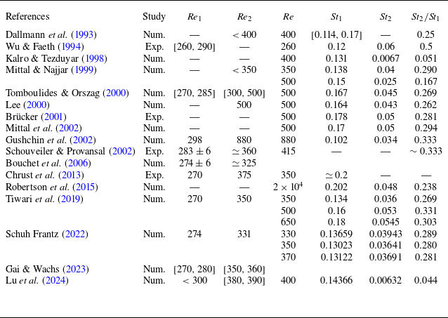
 Re1
Re1 Re2
Re2 St1
St1 St2
St2 St2/St1
 Re
Re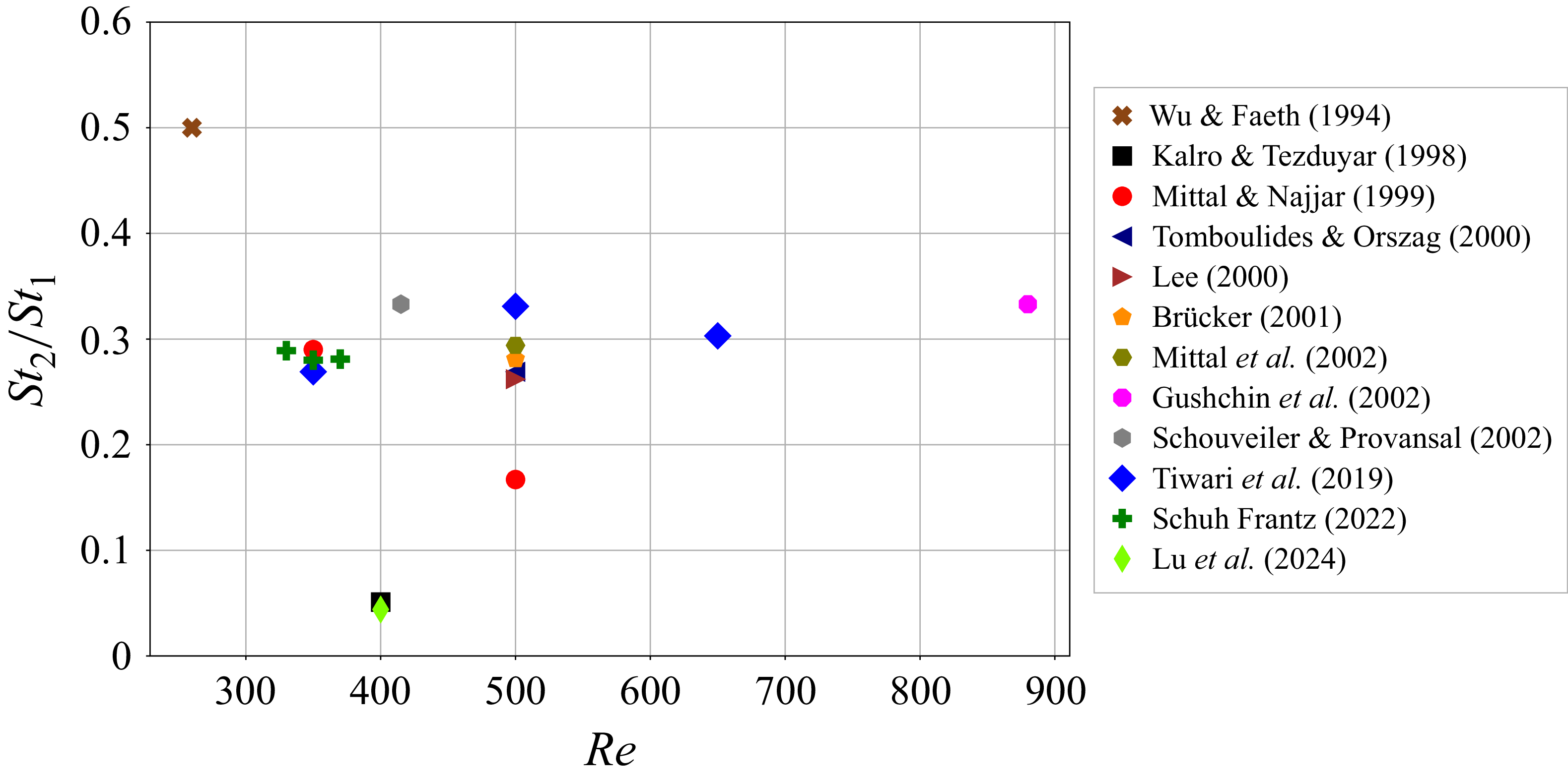
 St2/St1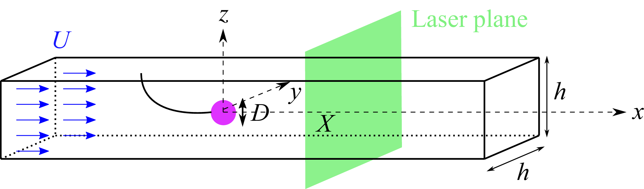
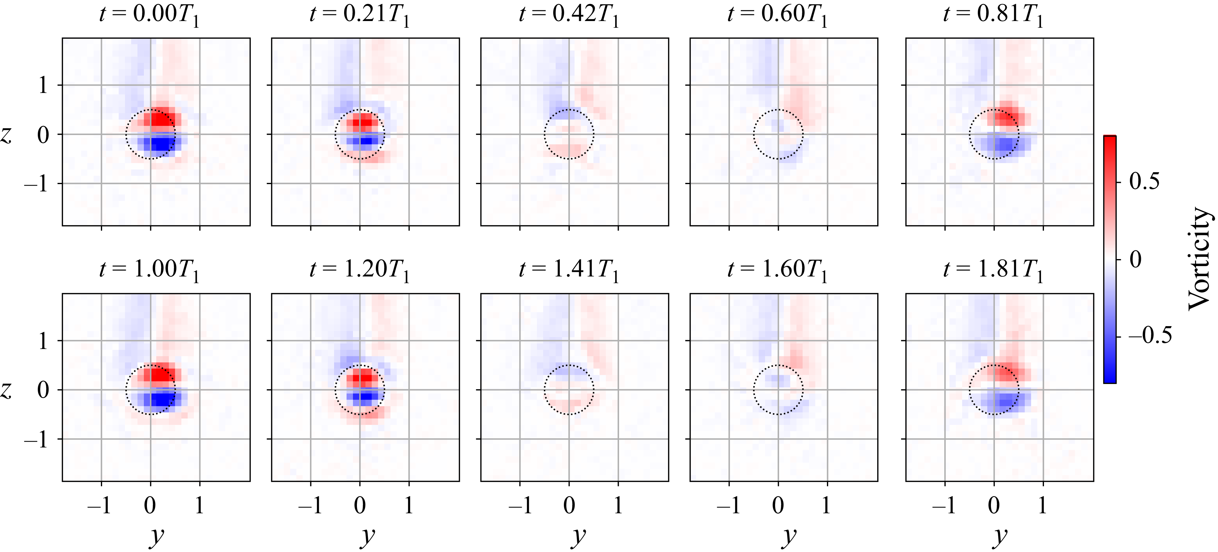
 Re=322
 X=3
X=3 yz
yz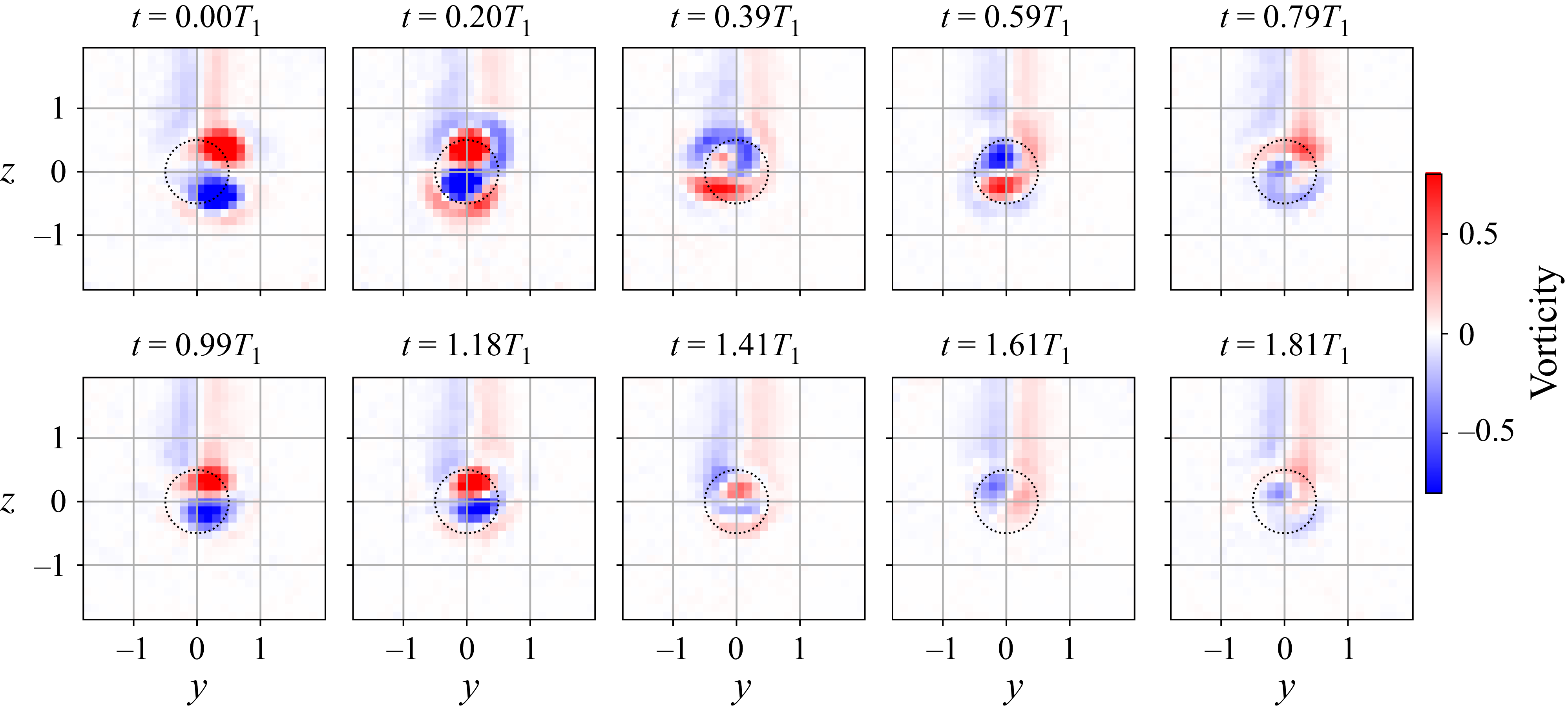
 Re=409
 X=3
X=3 yz
yz
 (Gy,Gz)
 X=3
X=3 60s
60s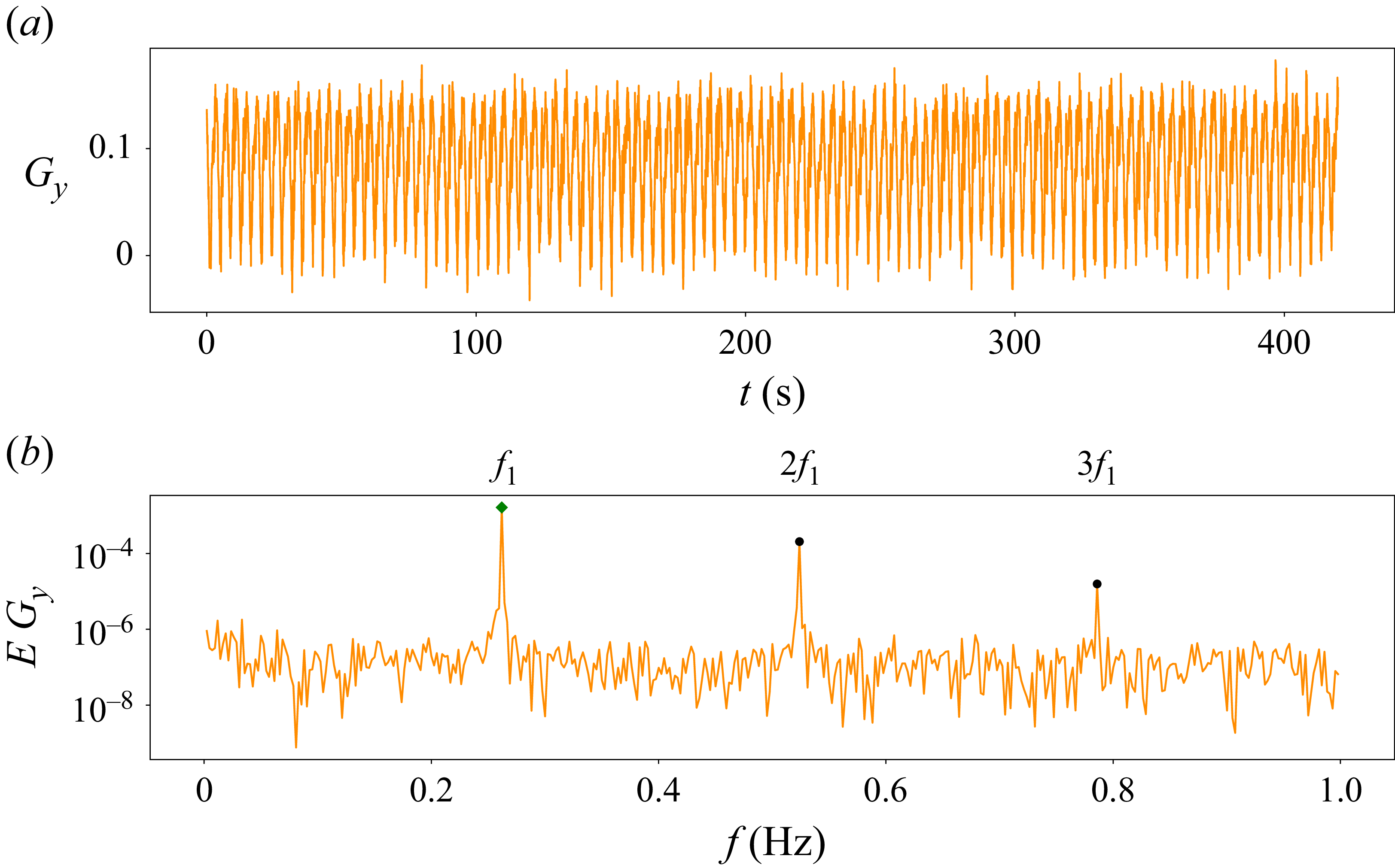
 Re=322
 X=3
X=3 Gy
Gy y
y Gy
Gy f1=0.262±0.003Hz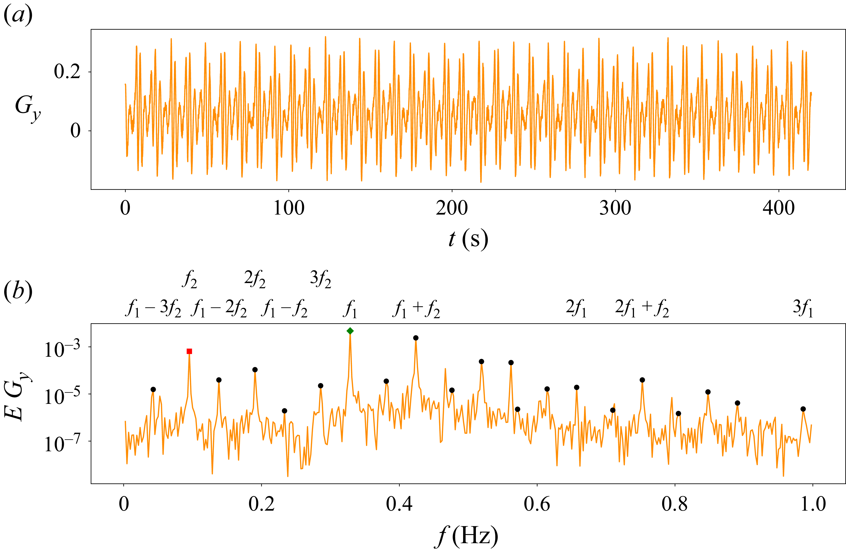
 Re=409
 X=3
X=3 Gy
Gy y
y Gy
Gy f1
f1 f2
f2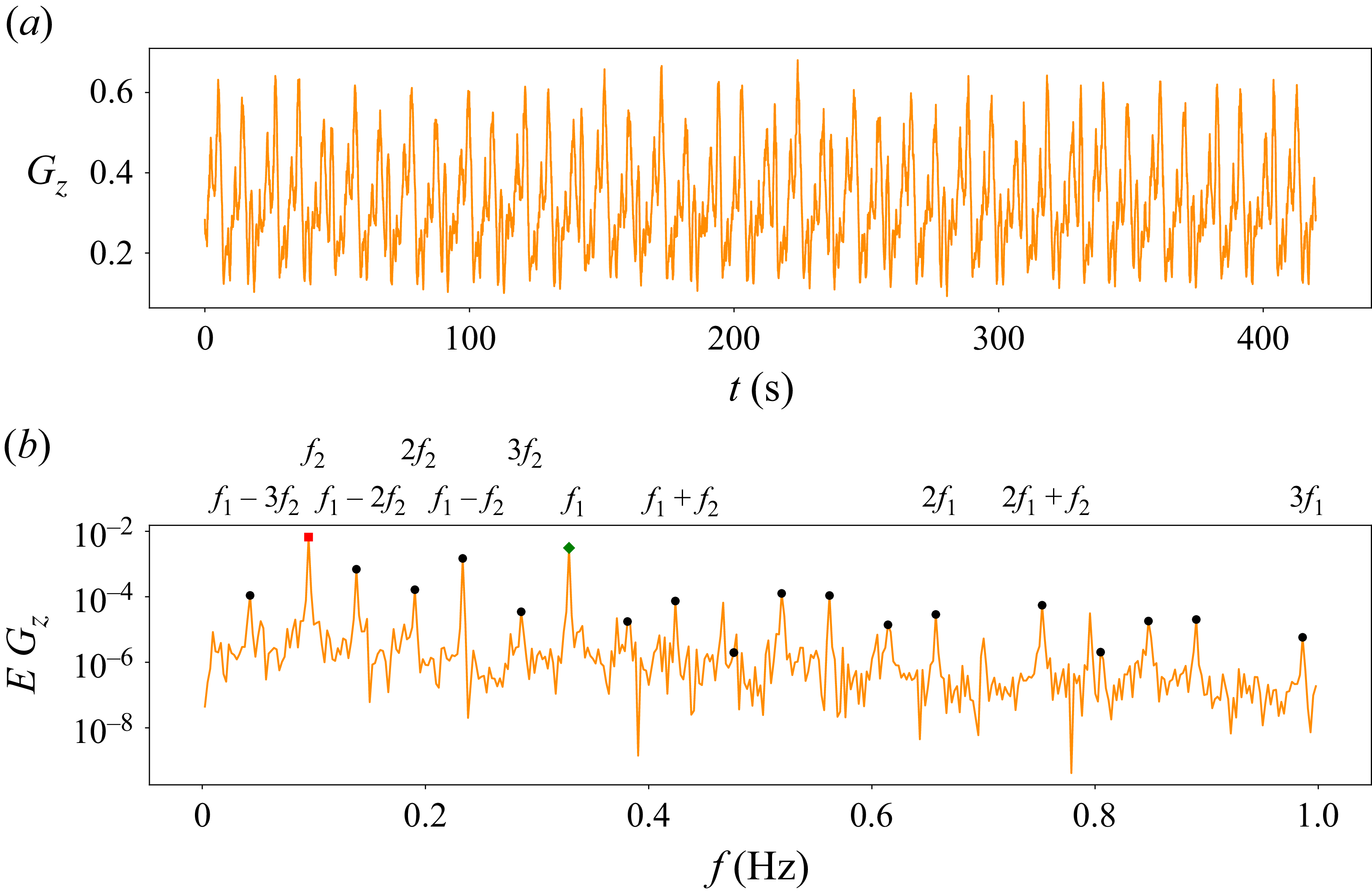
 Re=409
 X=3
X=3 Gz
Gz z
z Gz
Gz f1
f1 f2
f2
 f1
f1 Re∈[295,450]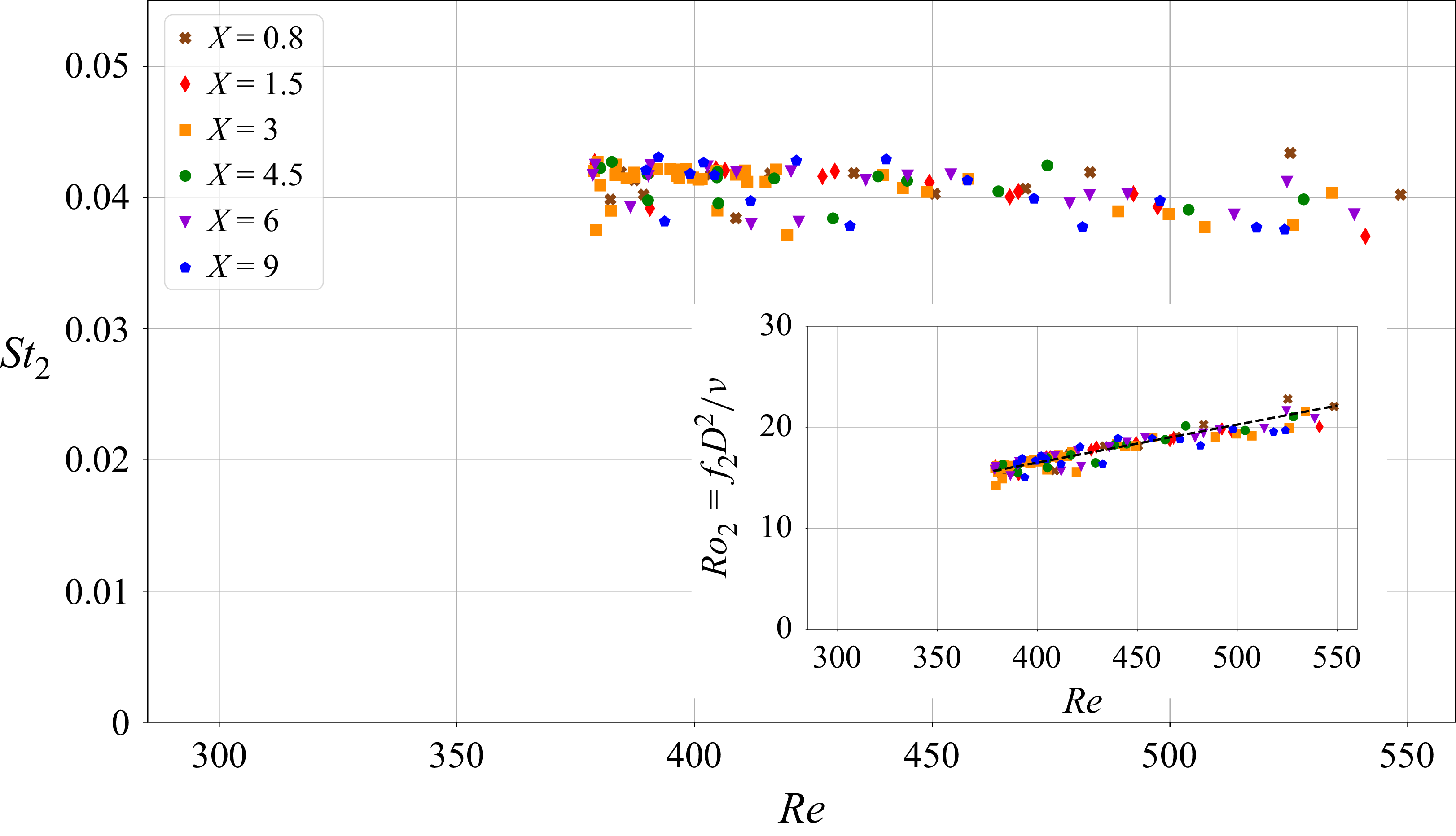
 f2
f2 Re∈[378;450]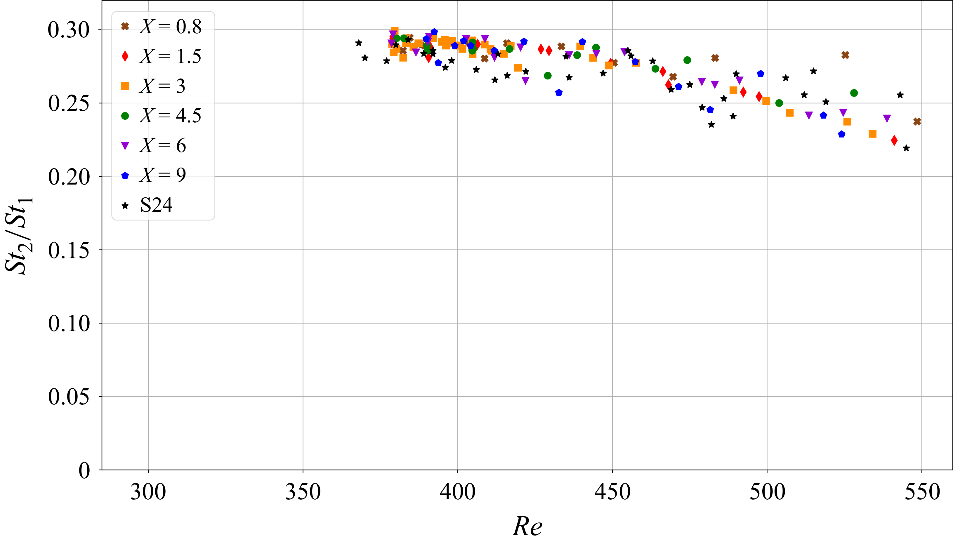
 St2
St2 St1
St1 24mm
24mm X=3
X=3
 1Hz
1Hz X=3
X=3 7T1
7T1 T1
T1
 Re=409
 f1
f1 f2
f2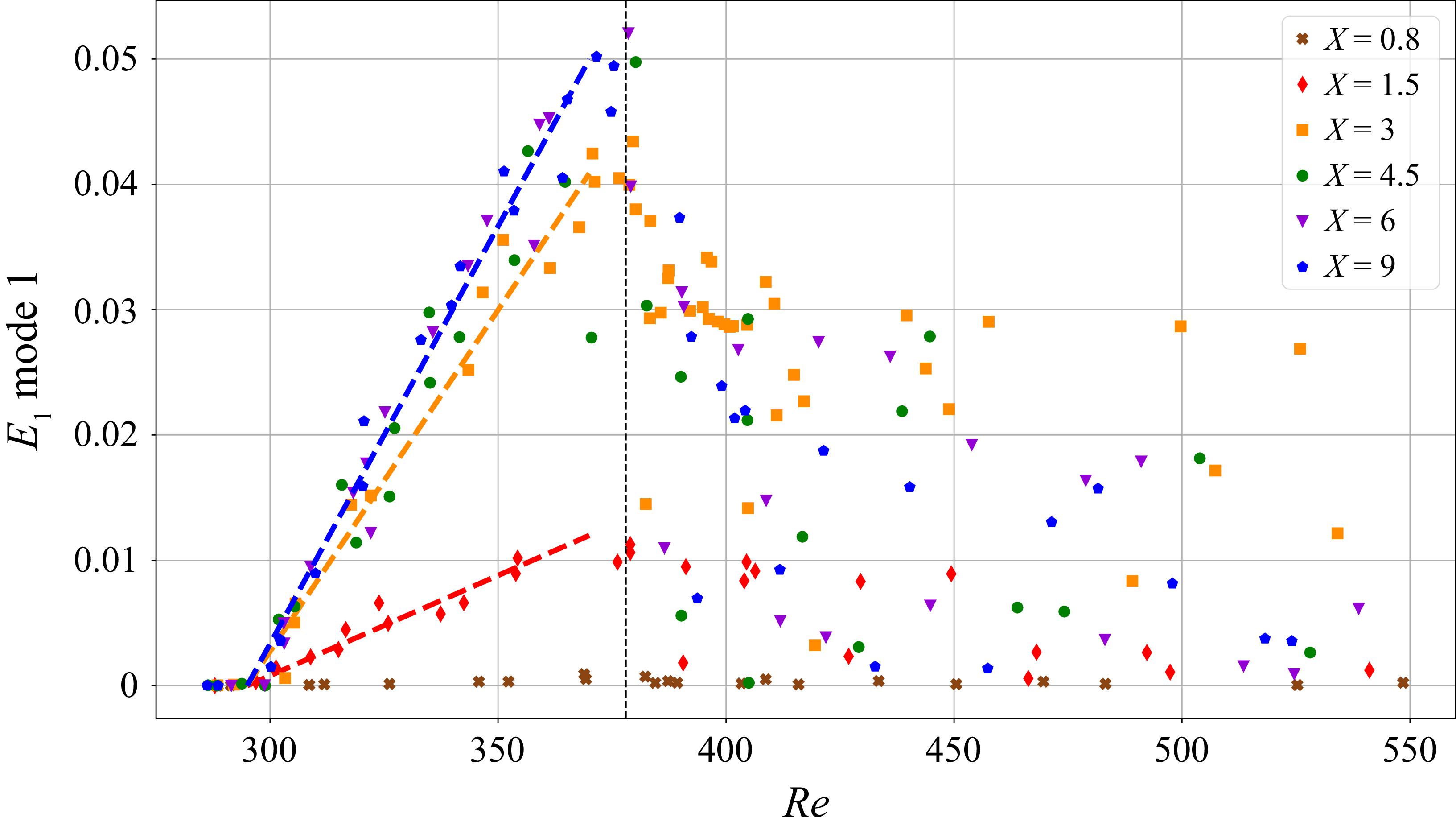
 St1
St1 Re2
Re2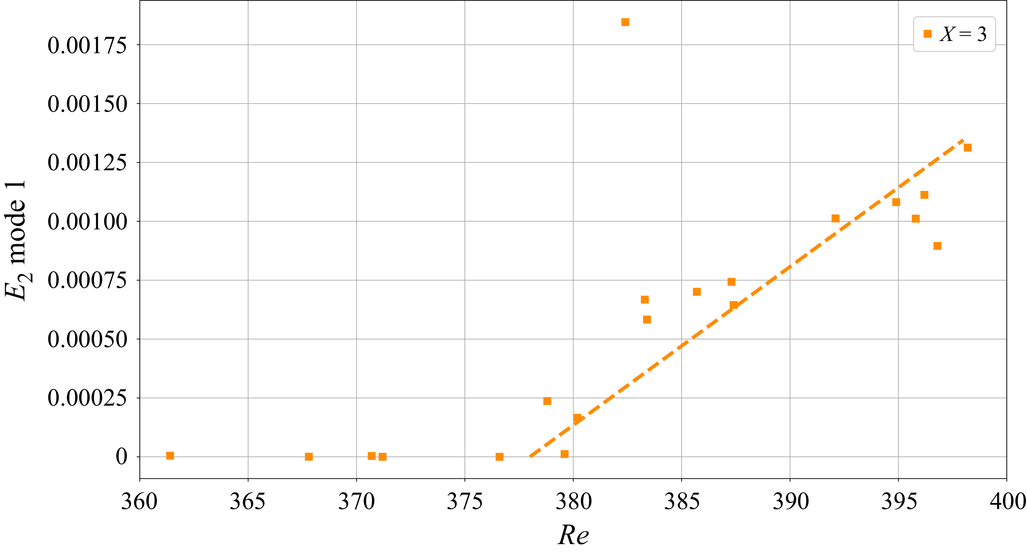
 St2
St2 X=3
X=3 Re∈[378,398]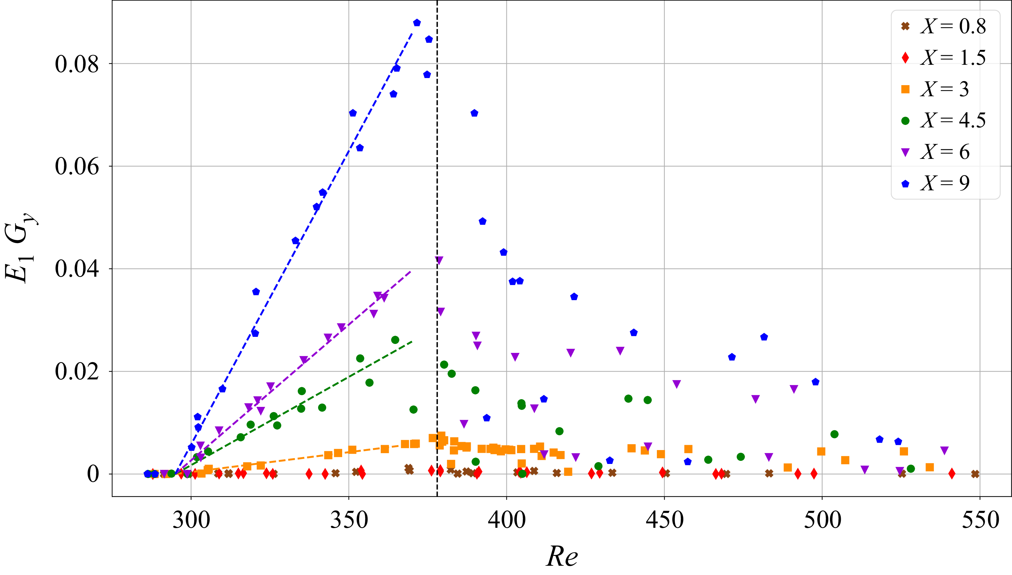
 St1
St1 Gy
Gy Re2=378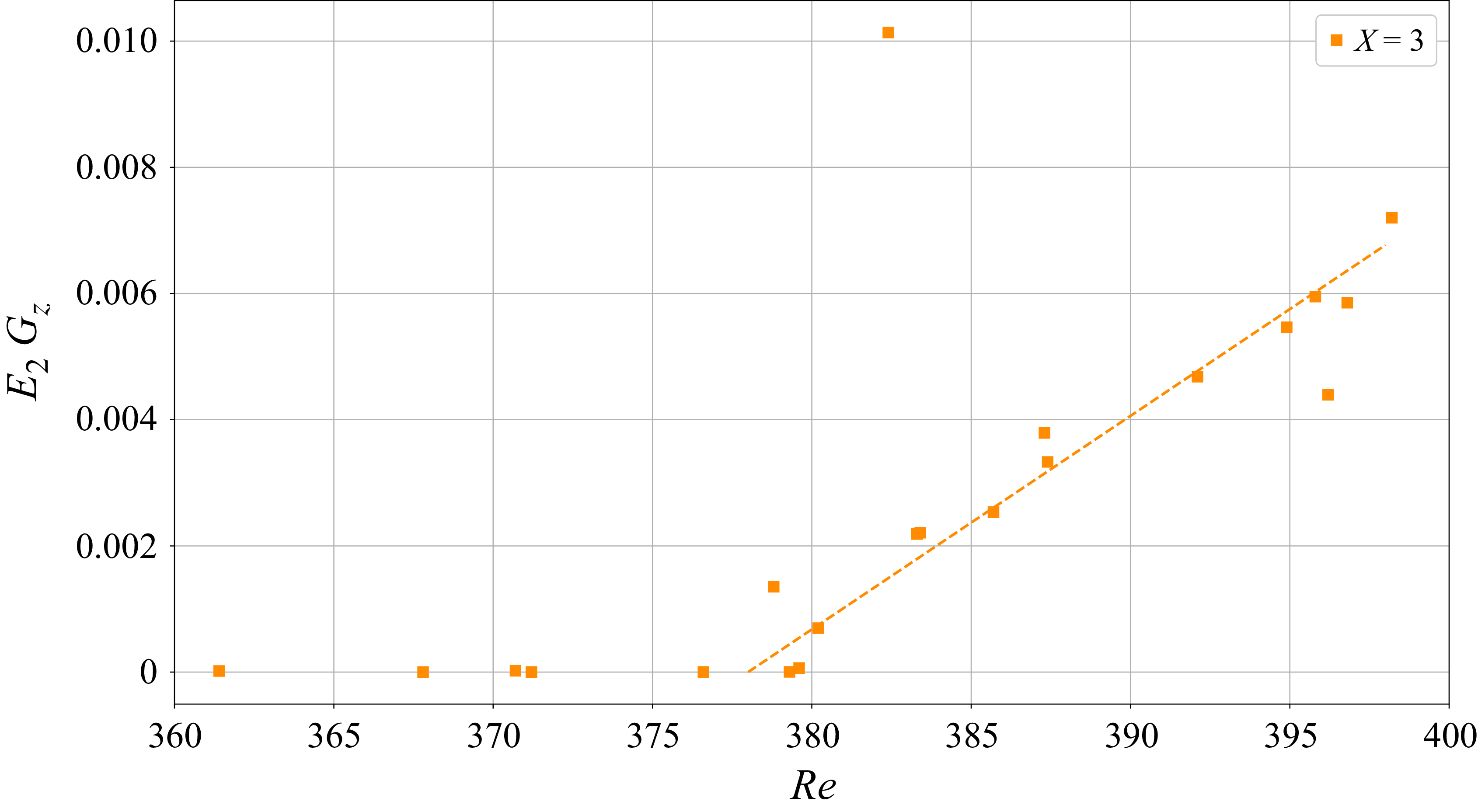
 St2
St2 Gz
Gz X=3
X=3 Re∈[378,398]
 f1
f1 f2
f2 Re=409
 X=3
X=3 T2
T2 T2=1/f2
 f1
f1 f2
f2 Re=409
 X=6
X=6
 f1
f1 f2
f2 Re=391
 X=6
X=6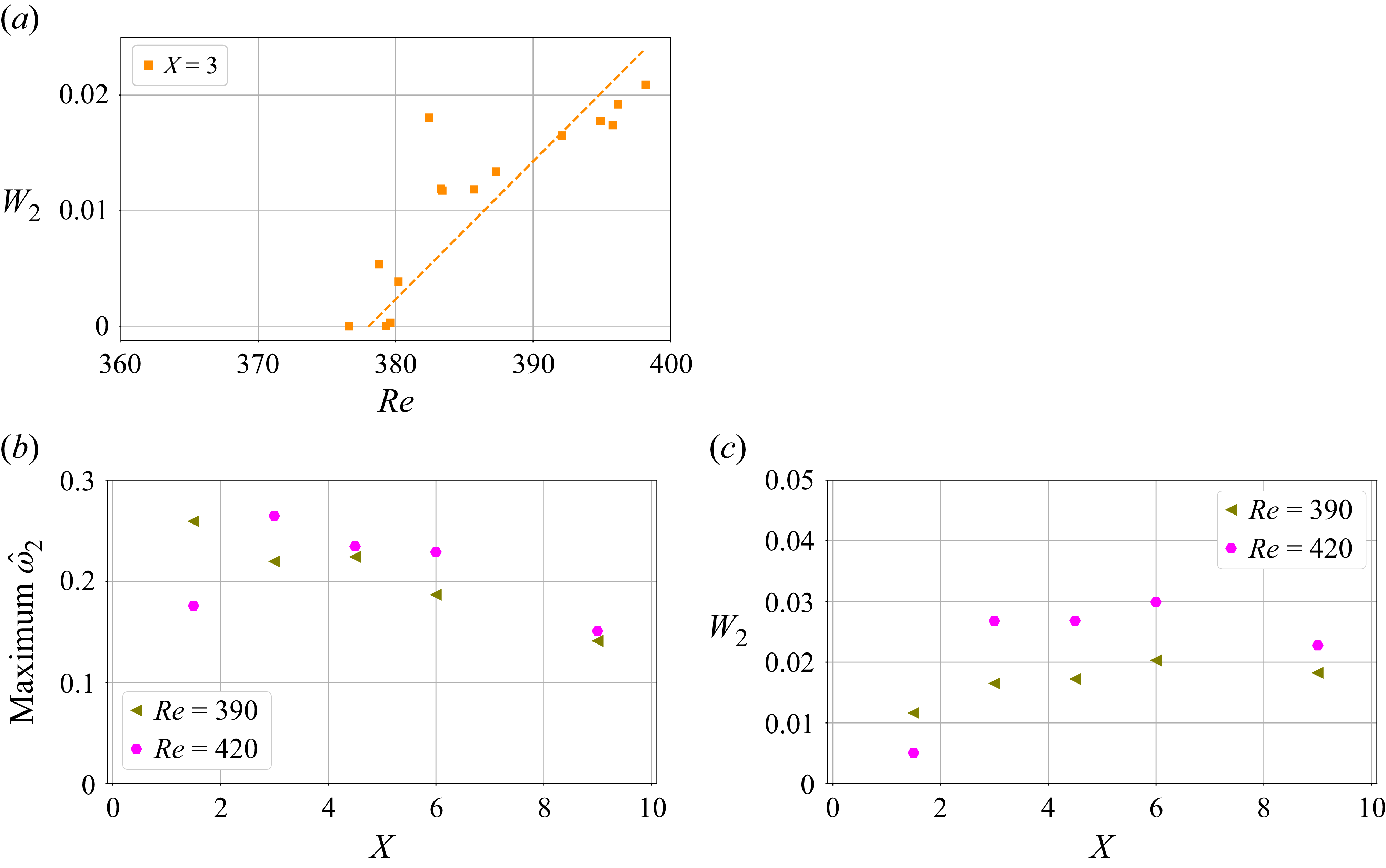
 W2
W2 X=3
X=3 f2
f2 X
X W2
W2 X
X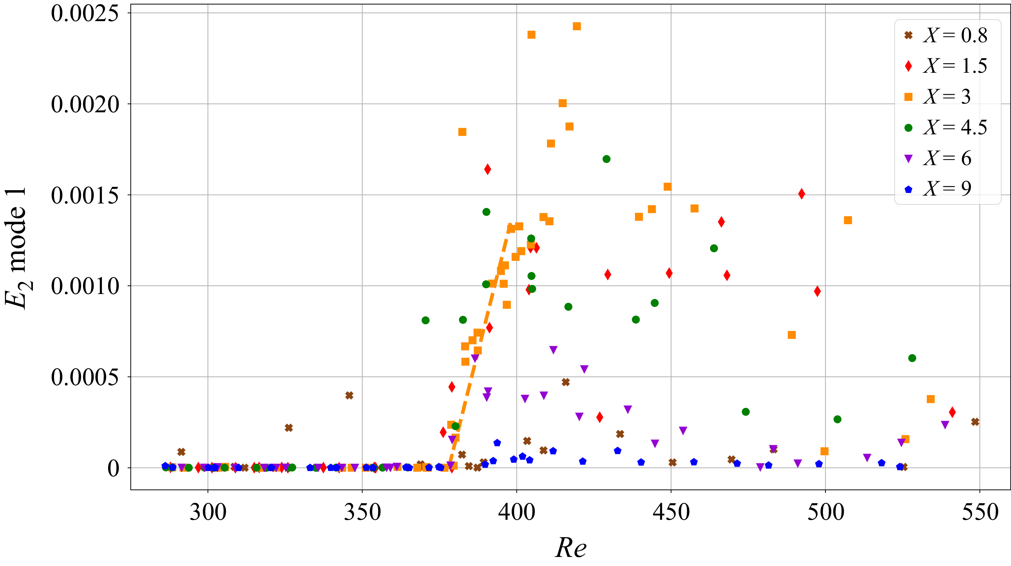
 St2
St2 X
X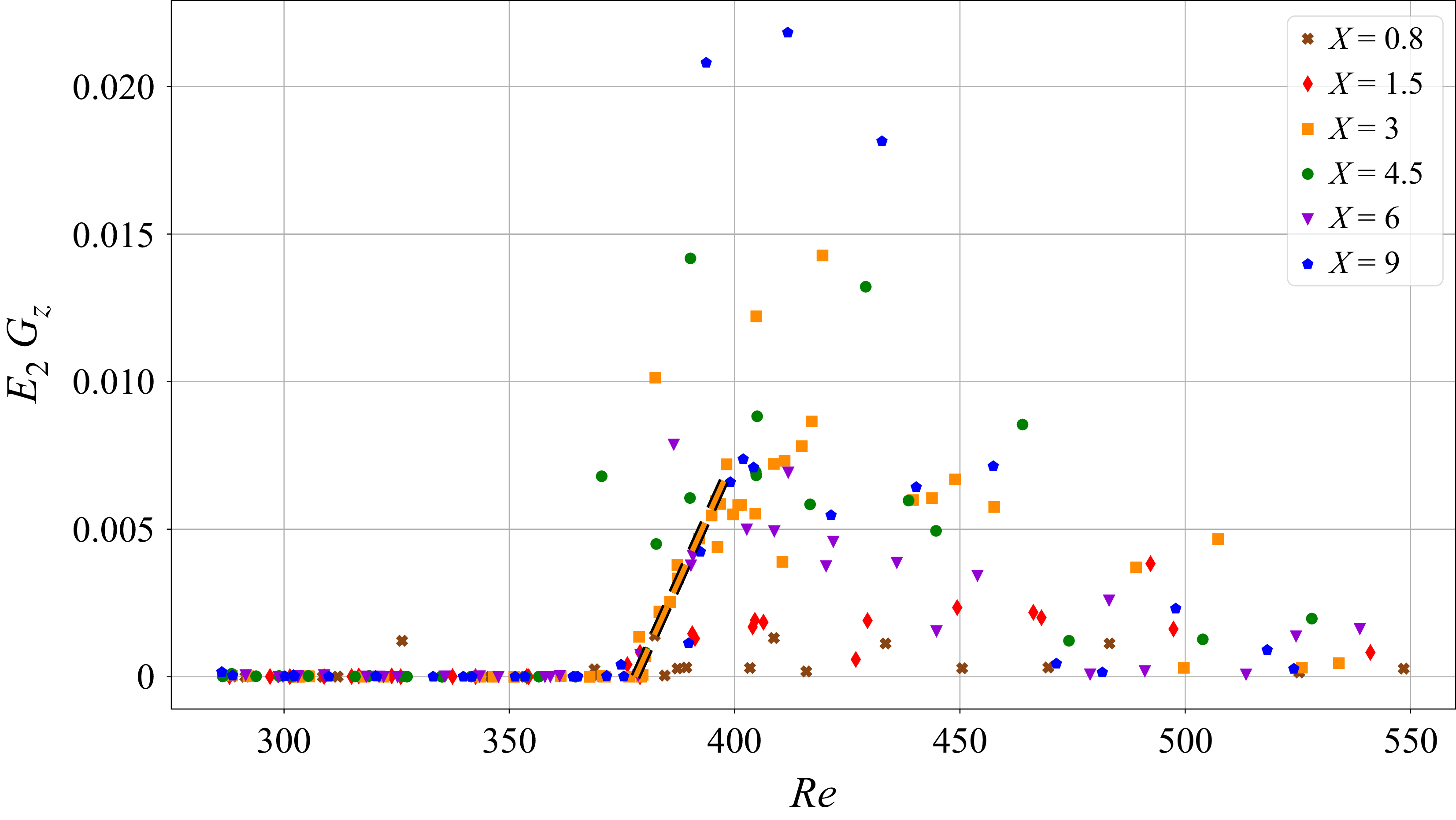
 St2
St2 Gz
Gz X
X Re
Re


 Open access

