


1. Introduction
In Reference NyeNye’s (1976) jökulhlaup theory, water from a flood lake drains in a subglacial channel whose size evolves to govern the drainage hydrograph. His theory ignores glacier flow due to basal sliding, which may respond to changing subglacial water pressures during floods. Such coupling between floods and ice dynamics is observed in alpine jökulhlaup systems as ‘ice-motion’ events, such as speed-up (Reference Anderson, Walder, Anderson, Trabant and FountainAnderson and others, 2005; Reference Mayer, Lambrecht, Hagg, Helm and ScharrerMayer and others, 2008; Reference Riesen, Sugiyama and FunkRiesen and others, 2010; Reference Sugiyama, Bauder, Riesen and FunkSugiyama and others, 2010; Reference Bartholomaus, Anderson and AndersonBartholomaus and others, 2011) and uplift (e.g. Reference Anderson, Walder, Anderson, Trabant and FountainAnderson and others, 2005; Reference Sugiyama, Bauder, Huss, Riesen and FunkSugiyama and others, 2008; Reference MagnussonMagnússon and others, 2011) during flood growth followed by deceleration or reversal in ice flow during flood recession (Reference Anderson, Walder, Anderson, Trabant and FountainAnderson and others, 2005; Reference Sugiyama, Bauder, Huss, Riesen and FunkSugiyama and others, 2008; Reference MagnussonMagnússon and others, 2011). This coupling also occurs in ice sheets. Studies in Greenland show that surface meltwater routed via supraglacial lakes and moulins to the bed can cause short-term changes in surface velocity (Reference Zwally, Abdalati, Herring, Larson, Saba and SteffenZwally and others, 2002; Reference DasDas and others, 2008) and seasonal ice speed-up (Reference BartholomewBartholomew and others, 2011). These observations raise the question of whether and how much climate-warming induced changes will increase the long-term ice flux (e.g. Reference SchoofSchoof, 2010; Reference Sundal, Shepherd, Nienow, Hanna, Palmer and HuybrechtsSundal and others, 2011). Both alpine marginal lakes and supraglacial lakes are reservoirs whose water balance depends on climate, and drainage–ice-flow coupling in both types of system involves rapid, high-magnitude variations in subglacial discharge; Nye’s theory offers a foundation for modelling the physics of this coupling.
Here, considering alpine jökulhlaups only, we present a consistent model of this coupling by extending several strands of previous work. A key feature of Reference NyeNye’s (1976) theory is the growth of channel discharge through positive feedback with melt enlargement of the channel during the rising flood stage. As the lake drains and its level drops, reduced subglacial water pressure promotes channel closure and flood termination. Numerical solution of this model (e.g. Reference Spring and HutterSpring and Hutter, 1981; Reference ClarkeClarke, 1982, Reference Clarke2003; Reference NgNg, 1998; Reference FowlerFowler, 1999, Reference Fowler2009; Reference Ng and BjörnssonNg and Björnsson, 2003; Reference Kessler and AndersonKessler and Anderson, 2004; Reference Ng, Liu, Mavlyudov and WangNg and others, 2007) shows that simulation of jökulhlaup discharge requires full coupling between sub-glacial drainage and the lake – defined by the two conditions: (1) water flux at the channel inlet equals the lake outflow, and (2) the lake-water depth controls the water pressure at the channel inlet (correctable, in the case of a subglacial lake covered by an ice shelf, for over-pressurization due to vertical shear stresses in the shelf; Reference Evatt and FowlerEvatt and Fowler, 2007). Full coupling is also necessary in any extended model incorporating ice flow and aimed at predicting flood hydrographs.
Recent numerical studies have highlighted the rich hydrological and glacier-dynamical behaviour that can arise when Nye’s evolving channel coexists with a distributed drainage system. Reference Flowers, Björnsson, Palsson and ClarkeFlowers and others (2004) showed that lake water injected into a subglacial water sheet, that in turn feeds and rapidly enlarges a channel, can explain the fast-rising discharge seen at the start of the 1996 Grímsvötn (Iceland) flood hydrograph (Björnsson, 2002), not reproducible by Nye’s model (Reference JóhannessonJóhannesson, 2002). Reference Pimentel and FlowersPimentel and Flowers (2011) added other processes to this description – high-order glacier dynamics, basal sliding, ice hydraulic fracture and ice uplift – to explore several glacio-hydraulic scenarios. Since these studies did not focus on flood dynamics, they prescribed a known discharge at the top end of the channel, neglecting condition (2) above. In our model, we use full coupling to let the channel discharge evolve freely, so that the response it causes in distributed drainage and ice flow can feed back and influence lake drainage. The model is used to examine jökulhlaup characteristics and glacier motion during floods. We study specifically whether the incorporation of distributed drainage and ice motion into Nye’s theory alters the floods’ hydrographs, their initiation threshold and recurrence. Impact of ice motion on supraglacial lake drainage is also conceivable in the ice-sheet scenario, where a supraglacial lake or a moulin acts as a reservoir with more complex geometry than an ice-marginal lake.
A further research strand provides us with a model of distributed drainage and sliding. Reference Hewitt and FowlerHewitt and Fowler (2008) proposed a theory to explain seasonal waves on glaciers. By linking channelized subglacial drainage to cavity drainage with sliding, they showed that imposing periodic meltwater input to this system can cause oscillations in ice flow resembling observations. We adopt some of their cavity system equations below, but couple them to a fully dynamic channel, itself pressure-coupled to a lake. Hewitt and Fowler’s way of forcing the system also inspires us to view the background water supply to the cavities (MC) as an environmental factor behind jökulhlaups.
Our model and its numerical solution are described in Section 2. To gain general insights into alpine and ice-cap Jökulhlaup systems, we assume simplified lake and glacier geometry representative of these systems, rather than tailor parameters for a given lake. Section 3 reports our numerical experiments. We show that water transfer from the cavities to the channel can suppress the growth of recurring floods, and we study the spatio-temporal pattern of glacier flow during Jökulhlaups. We find that basal sliding is strongly sensitive, but the flood hydrograph weakly sensitive, to MC. We discuss these findings alongside field observations at several Jökulhlaup lakes in Section 4.
2. Mathematical Model
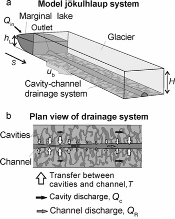
Figure 1 shows our system. A lake feeds a subglacial channel of length s0, which exchanges water with a distributed system of linked cavities outside it; the cavities influence and are influenced by sliding. We denote distance down-glacier from the lake by s, time by t, and use subscripts R (for Rothlisberger) and C to label channel and cavity variables, respectively. While we aim to couple flood and ice-flow dynamics, three specific ‘couplings’ occur in the model: between the lake and subglacial drainage, between the channel and cavities, and between cavities and sliding.
Diagram of our model Jökulhl aup system.
2.1. Channelized drainage
Reference NyeNye (1976) envisaged the channel cross-sectional area SR to evolve under the competition between melt enlargement and creep closure. We use Reference FowlerFowler’s (1999) version of his model, which allows the discharge QR to go negative (e.g. when the channel drains into the lake between floods), and where the equations for channel evolution, mass conservation and momentum conservation, are, respectively:
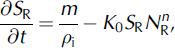

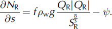
In Eqn (1), the two terms on the right represent melting and closure. The mass melted per unit channel length per unit time, m, is given by m = ( + <9NR/<9s)|QR|/L; this expression assumes that potential energy is instantaneously dissipated through friction to melt the channel walls. NR is channel effective pressure (=Pi-PR, with Pi being ice overburden pressure, PR being channel water pressure), pw and pi are water and ice densities, g is gravity, L is latent heat of fusion of water and f is hydraulic roughness (f= n’2(l2/SR)2/3 ?s0.07 m–2/3 s2 for a semicircular channel with wetted perimeter land Manning’s roughness coefficient n’=0.1 m–1/3s). The constants n = 3 and K0 = 10–24 Pa-3 s–1 pertain to temperate ice rheology (Reference FowlerFowler, 1999); K0 accounts for the assumed semicircular cross section of the channel.
The term Tin Eqn (2) represents the rate of water transfer into the channel from the cavities (volume flux per unit distance). Following Reference Hewitt and FowlerHewitt and Fowler (2008) we model it as proportional to the pressure difference between these drainage components:

where NC is the cavity effective pressure and k is a connectivity constant (we adopt Hewitt and Fowler’s value 10–9m2 s–1 Pa-1). R k is a dimensionless factor used in our experiments (Section 3.1) for varying the transfer rate Rkk that saves us from writing out its units each time.
Equation (3) derives from Manning’s friction formula and is the basic hydraulic gradient, given by
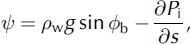
where 4>b is the glacier bed slope. We assume a with uniform thickness H (Fig. 1), so is constant.
Equations (1-3) neglect the lake’s internal energy that could enhance the channel melt rate m (Reference ClarkeClarke, 1982), so this model assumes lake and subglacial water temperatures equal to the pressure-melting point. Also, as NR and NC stay positive in our simulations, we do not model channel enlargement caused by ice uplift when NR
2.2. Lake evolution
The lake depth hL (Fig. 1) evolves with water input (Qin) and outflow (QR at the channel inlet) following the continuity equation
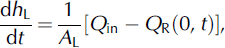
where AL is uniform lake area. Equation (6) expresses condition (1) of our full coupling (Section 1). According to condition (2) of our full coupling, the hydrostatic lake pressure fixes the channel-inlet effective pressure to be

at all times, and this provides a boundary condition for NR in Eqn (3).
2.3. Linked-cavity drainage and basal sliding
We follow Reference Hewitt and FowlerHewitt and Fowler (2008) in using a pseudo-steady description for the geometry of the cavities, with a conservation equation for the water flux through them and a sliding law. For sliding at velocity ub over bed obstacles of height R, Reference WalderWalder (1986) showed that the typical cavity cross-sectional area is

where γ ≈ 0.32 and k1 ≈ 1.1 are constants, and that the water discharge through the cavity system, QC , depends on hydraulic gradient (just as for the channel) so that QC and SC are related via

We adopt a power law to describe sliding,

(e.g. Reference BindschadlerBindschadler, 1983), where p = 4, q=1, cs is a constant dependent on bed roughness ( « 2 x 10–20 ms–1 Pa-3; Reference Hewitt and FowlerHewitt and Fowler, 2008), and Tb is the basal shear stress assumed to balance local driving stress pigHsincj)s where 4>s is glacier surface slope (Reference Cuffey and PatersonCuffey and Paterson, 2010). Following Reference WalderWalder (1986) and Reference KambKamb (1987), we assume that the sliding control on cavity size (the first of the two terms enclosed by the square brackets in Eqn (8)) dominates frictional heating (the second term). On neglecting the latter term, eliminations between Eqns (8) and (10) lead to
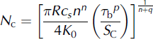
and
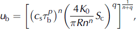
which give the cavity effective pressure and sliding velocity in terms of SC. For the bed obstacle height R, we use Reference WalderWalder’s (1986) value of 0.1 m.
A final equation describes water conservation in the cavities:

where MC is the background water supply to the cavities from basal- and surface-derived melt. We assume that the channel receives meltwater only via the cavities (through T) and none directly via moulins or other englacial routes.
1Equations (-6), (9), (11a), (11b) and (12) complete our model. In essence it describes the coupled evolution of channel size, cavity size, and lake level. SR, QR, NR, T, SC, QC, NC and ub are functions of t and s, while hL is a function of t only. This model differs from Hewitt and Fowler’s not just in its inclusion of the lake and a channel that evolves at a rate dictated by melt and ice creep, but also in using the total hydraulic gradients > +<9NR/<9s and + dNC/ds to drive channel and cavity flow (rather than alone). Four boundary conditions are needed in Eqns (2), (3), (9) and (12) for determining the discharge and pressure in these systems. For the channel we impose the condition in Eqn (7) and NR = 0 at the terminus (s = s0). For the cavities, an equation like (7) could be used to couple the cavities and the lake hydraulically. Preliminary investigations indicate that interesting dynamics result from this coupling, but a full exploration of its consequences is beyond our scope here. Instead, for simplicity, we isolate the cavities from the lake, by assuming that NC at the lake (s = 0) and at the terminus (s = s 0) are both constant, «1 x 10⁵ Pa. Although this value may seem arbitrary, the qualitative features of our results reported below are not sensitive to its size.
Our assumption of pseudo-steady cavity geometry is motivated by the supposition that, unlike in channels, the cavity system’s effective pressure-discharge relationship will be negative whether the system is steady or not, and motivated by the lack of unsteady cavity drainage models that are strongly verified by subglacial observations. However, the potential limitations of our model need to be recognized. Since, in reality, cavity size will not react instantaneously to pressure changes, our model overestimates the role of water storage in cavities when water transfer changes rapidly and neglects the lag of peak cavity size behind peak cavity water pressure. In such situations, the model will underestimate actual NC and ub variations. Also, our model precludes investigation of a possible negative feedback between cavity size and pressure suggested by Reference Bartholomaus, Anderson and AndersonBartholomaus and others (2011). In a recent theory, Reference Hewitt, Schoof and WerderHewitt and others (2012) have tried to overcome these limitations by modelling the cavity system dynamically as a sheet with a cavity evolution equation analogous to Eqn (1).
2.4. Method of numerical solution
We solved the equations with the finite-difference method on a discretized space-time domain. The forward Euler method was used to integrate Eqns (1), (6) and (12), with upwinding for the spatial derivative in Eqn (12). When calculating results at the next time-step, we first used variables from the current time-step to update the lake depth hL and cavity area SC, from which the sliding velocity ub, cavity discharge QC and pressure NC could be found by Eqns (11) and (9). Turning to the channel, we then used Eqn (1) to update SR, and used SR in Eqns (2) and (3) (with their boundary conditions and NC at the new time) to find the discharge and pressure distributions QR and NR at the new time-step. In this boundary-value problem, where (and whether) QR switches sign along the channel is not known a priori. To overcome this we solved Eqns (2) and (3) by two nested iteration loops. In the inner loop, a guess of the lake outflow QR(s = 0) at the new time was used as the boundary condition for integrating Eqn (2) into s>0. We used dynamic relaxation for Eqn (2) and introduced a fictitious sdQR/dt to its left-hand side, and iterated QR to steady state on the fast (e) timescale. This inner loop thus yields the QR and NR distributions simultaneously, including the channel effective pressure at its inlet, NR(s= 0). Generally, QR(s = 0 ) and NR(s=0) at the new timestep from this loop mismatch the lake condition in Eqn (7). In the outer loop, we use the Newton-Raphson method to correct the guess of QR(s = 0) iteratively (letting the inner loop converge each time) to obtain the match.
3. Results of Numerical Simulations
We report here numerical experiments made with the model to study (1) the cyclicity of recurring floods, (2) variations in ice flow in each Jökulhlaup cycle, and (3) sensitivity of these variations to the cavity water supply, MC. Throughout, a lake with area AL = 5 km2, and a glacier described by parameters s0 = 10 km, H= 100 m and sin0s = sin^b = 0.01, are assumed. These values pertain to Merzbacher Lake and South Inylchek Glacier, Kyrgyzstan (Reference Ng and LiuNg and Liu, 2009), and lead to « 100 Pa m–1 and Tb « 9 kPa.
3.1. Flood cycles
Nye’s model formulated with only time dependence and no spatial dependence can simulate recurring floods, but their size grows indefinitely with time through a feedback between decreasingly small channel size and increasing highstand and peak discharge (Reference NgNg, 1998; Reference Ng and BjörnssonNg and Björnsson, 2003). In reality many Jökulhlaups terminate through complete emptying of the lake, which would interrupt such unbounded growth, but Reference Ng and BjörnssonNg and Björnsson (2003) also found this behaviour when simulating floods from Grímsvotn, Iceland, which does not empty (Björnsson, 2002). Consequently, unbounded flood growth is seen as an intrinsic weakness of some Jökulhlaup models. Reference FowlerFowler (1999) showed that model flood cycles remain bounded if spatial dependence is included, the channel receives a uniform meltwater supply and the basic hydraulic gradient near the lake is negative (e.g. due to retrograde ice-dam surface slope towards the lake - a ‘topographic seal’). Whether uniform channel supply and a topographic seal are necessary conditions for bounded flood cycles has remained unexplored. As our model treats how the channel captures subglacial water in more detail than Fowler’s model and uses a positive basic hydraulic gradient everywhere, we address this by asking whether we can simulate stable flood cycles.
Figure 2 shows the simulated time series from a set of model runs, each spanning 15 model years and conducted with an initial lake depth of 30 m (hL at t=0), a constant lake-water input Qin=10m3s–1, a constant background water supply to cavities M C = 1 x10⁻³m2s–1 , and several values of the parameter Rk between 0 and 1. Rk = 0 and Rk=1 refer to total hydraulic isolation and the hydraulic coupling used by Reference Hewitt and FowlerHewitt and Fowler (2008), respectively. The coupled lake-channel-cavity system oscillates in time, yielding asymmetric filling and draining cycles of lake depth (Fig. 2a, c, e and g) and corresponding floods in the channel discharge (Fig. 2b, d, f and h). In all runs, initially, the volume and peak size of successive floods increase with time in a transient response to initial conditions. When Rk<0.3, the lake’s post-flood ‘lowstand’ level decreases until the lake empties completely, interrupting the simulation (Fig. 2a-d). In contrast, when R k > 0 . 6 , the cycles become periodic and stable without emptying the lake (Fig. 2e-h). Runs using 0.3 <R k < 0.6 (not shown) show that increasing Rk delays the emptying of the lake as peak discharge is suppressed by increased cavity-to-channel water transfer.
Modelled lake level, hL(t) (left), and channel discharge at the lake, QR(0, t) (right), for Rk= 0, 0.3, 0.6 and 1. Cavity water supply, MC =1x10⁻³ m2 s–1.

These results go beyond Fowler’s to show that stable limit cycles occur when high T values allow the channel to capture water efficiently from the cavities and a water divide (or seal) to form between floods. The stabilizing effect of this transfer is evidenced also by the impact of Rk on the cycles: the higher is Rk, the shorter is their period and the smaller the flood volumes. Furthermore, we show that the channel can drain water into the lake at low lake levels and stable flood cycles can occur even if the basic hydraulic gradient is positive everywhere: a topographic seal is not a necessary condition for water divide formation.
3.2. Spatio-temporal evolution of sliding and drainage
The periodicity of stable cycles provides us with a common basis for studying individual floods and how their characteristics depend on model parameters, without the obstacles associated with initial conditions. Here we analyse the spatio-temporal behaviour of subglacial drainage and ice flow in the («1.5year long) flood cycle highlighted by the boxes in Figure 2g and h.
Figure 3 shows the simulated lake depth hL(t) and lake outflow QR(s = 0, t) (Fig. 3a), basal sliding velocity ub(s,t) (Fig. 3b) and rate of cavity-to-channel water transfer T(s, t) (Fig. 3c) through the cycle. Figure 3c is a map of Tover time and distance; a similar map is also used to plot ub(s, t) in Figure 4c, studied in Section 3.3. The hydrographic sequence here has been discussed by Reference FowlerFowler (1999). In Figure 3b, the time before point A (and after point E of the last cycle) is the lake-refilling phase between successive floods. At point A, high lake level moves the subglacial ‘seal’ (water divide in the channel) back to the lake, initiating the flood and allowing Nye’s positive feedback to enlarge the channel. B marks the time of the lake-level highstand when the flood’s growing discharge instantaneously matches the lake-water input. C and D mark the flood peak and the post-flood lake lowstand, respectively.
Evolution of (a) lake level, hL(t), and channel discharge at the lake, QR(0, t); (b) sliding velocity, ub(s, t); and (c) cavity-channel water transfer rate, T(s, t) in the limit cycle indicated by the boxes in Figure 2g and h. MC=1 x 10⁻³ m2s–1, Rk = 1.

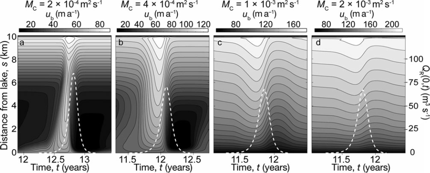
Sliding velocity ub(s, t) (filled contour maps) and channel discharge at the lake QR(0, t) (white dashed lines and right-hand vertical axis) in one limit cycle for (a) MC=2 x 10⁻⁴m2s–1, (b) MC=4 x 10⁻⁴m2s–1, (c) MC=1 x 10⁻³ m2s–1 and (d) MC=2 x 10⁻³m2s–1.
Regarding ice motion, Figure 3b shows similar responses in ub at different positions on the glacier. ub rises gradually as the lake fills, but accelerates rapidly after flood initiation (A) to peak soon after the time of the lake highstand (B). ub drops during the main flood (B to D) to a much lower velocity than during lake refilling, then increases again after flood termination (D to E). The durations of elevated and depressed ub are comparable. Spatially, ub rises monotonically with distance down-glacier, but its time variations at different positions are not precisely synchronous. Figure 3b shows that the peak and trough in ub propagate down-glacier at ?s250md–1 and «450md–1, respectively (see the dashed lines in Fig. 3c).
This sliding response can be explained by considering our model’s physics and is the direct result of the full coupling between the lake and the drainage system. Equation (11b) shows that ub varies directly with cavity size, SC. In turn, SC depends on how much water the cavities gain from the background supply MC and lose to the channel via water transfer, whose rate T increases with channel effective pressure, NR (Eqns (12) and (4)). The sliding response thus stems ultimately from changes in lake level, which, through its effect on the channel pressure, governs how fast the channel draws water from the cavities. The timing associations in Figure 3 between hL, T and ub confirm this explanation. When the lake fills between floods (E to A), reducing NR at the channel inlet, its hydrostatic pressure is not transmitted past the seal (located in Fig. 3c by the black line) to modulate Tand ub directly far down-glacier (further simulations show that this effect would be diminished if the cavities and lake were coupled hydraulically); there is a slight increase in ub only because the lake level weakly affects the distributions of NR and Tin the channel through its control on the migrating seal position. However, after the flood starts at t« 11.4 years, the seal’s absence means that the pressure transmission is unimpeded and able to reduce NR and T markedly down most of the channel (see descent into the dark trough in Fig. 3c); this causes the cavities to expand and accelerates sliding (A to B; 11.4< t< 11.7years). Later, as flood discharge grows, peaks, and recedes under Nye’s mechanisms (B to D, 11.7 < t < 12 years), the lake level drops rapidly, raising NR along the channel so that enhanced water transfer out of the cavities shrinks their size and decelerates sliding. After the seal re-forms at flood termination (E, t«12.2 years) we enter a new cycle. During the flood when the lake strongly modulates the cavity-to-channel water transfer, the nonlinear wave properties of Eqns (1-3) determine the propagation of changes in Tand ub down the channel.
3.3. Sensitivity to the cavity background supply, MC
Finally, we study how the ice-flow and flood evolution depends on the supply MC, which is the other control on cavity drainage beside T. For temperate glaciers, MC likely encompasses water reaching the bed from the surface, so it can be viewed as a proxy for weather conditions.
Figure 4a-d plot the maps of ub(s, t ) and time series of lake outflow from four model runs that assumed different values of MC between 2 x10⁻⁴ and 2x10⁻³m2s–1. Each plot’s duration is one flood cycle. The third run (Fig. 4c), identical to that discussed in Section 3.2, serves as the control. An enduring pattern in these runs is that the ice flow speeds up after flood initiation and begins to decelerate before the flood peaks. In the run with the lowest MC (Fig. 4a), the speed-up is very sudden and a strong compression wave (dub/ds<0) propagates down-glacier some 70 days prior to the flood peak (around 12.5 < t< 12.7 years).
Physically, we expect that decreasing MC reduces cavity size and discharge via mass conservation (Eqn (12)), and hence reduces the sliding velocity ub (Eqn (11a)). We see this trend in Figure 4a-d (note their different scales) as we move from right to left; however, the percentage variation in ub in the cycles increases. Figure 5 quantifies both trends by plotting the mean, maximum and minimum values of ub at 4 km from the lake in each cycle, including results from extra runs where MC is varied within the same range. As MC is raised, the mean value of ub increases but its maximum-to-mean ratio decreases.
Mean sliding velocity at 4 km from the lake, ub (circles and left axis), and peak lake discharge, QPK (crosses and right axis), for MC =2x10– 4 m2 s–1 to 2 x 10⁻³ m2 s–1. The top and bottom ends of the vertical lines indicate maximum and minimum ub at 4 km from the lake.
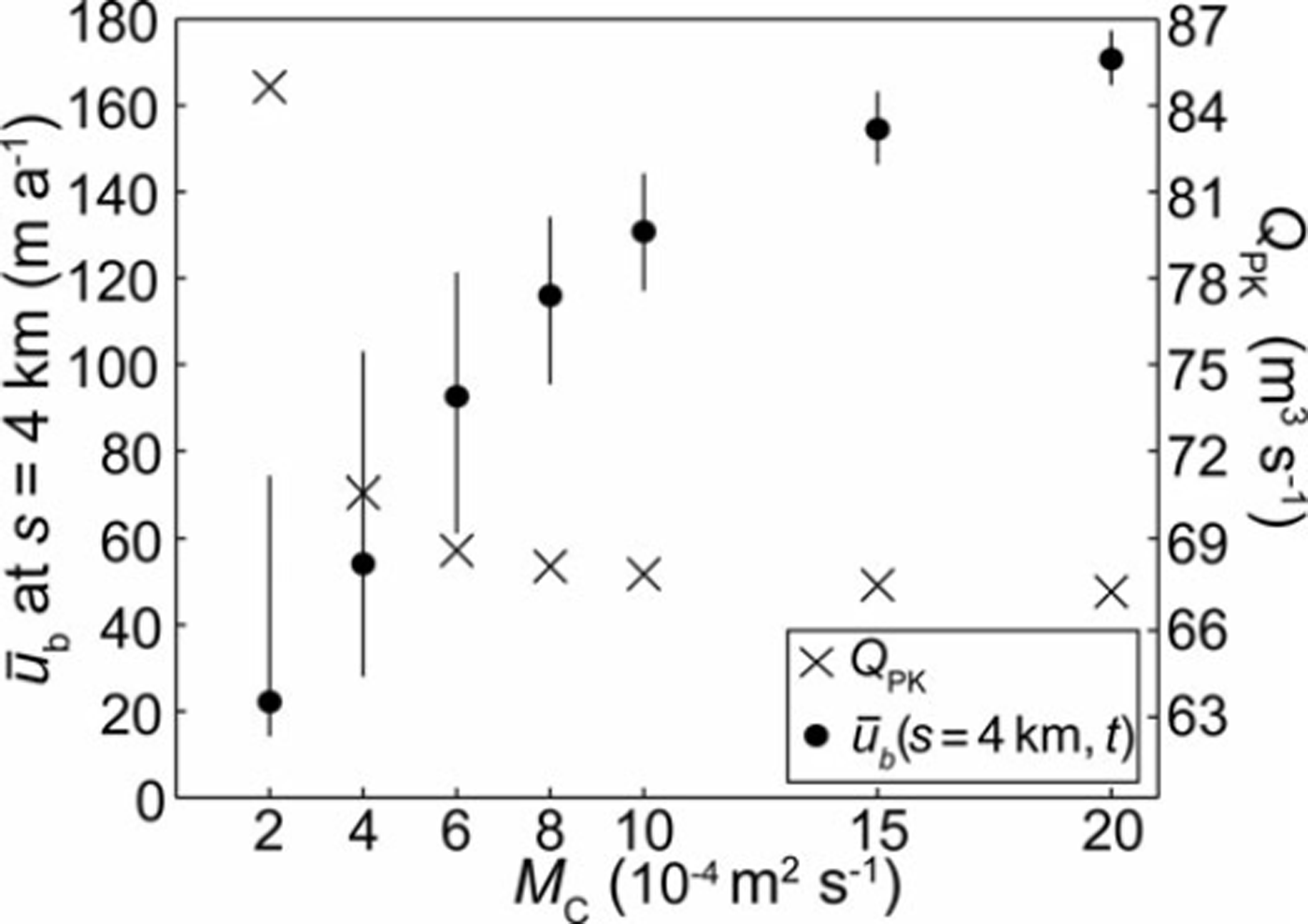
We expect two outcomes of decreased MC on cavity-channel interaction. One is increased dominance of the transfer term in the cavity mass conservation equation (Eqn (12)). This explains the variable maximum-to-mean ub ratio; when MC is large, the remaining, time-varying terms in Eqn (12), dQC/ds and T, are comparatively small and SC and ub vary less than when MC is small; then, SC and ub are modulated strongly because Tdominates the mass balance. In addition, when MC<4 x 10⁻⁴m2 s–1, the cavities collapse after the lake reaches its highstand due to high effective pressure in the channel, preventing significant reduction of ub below its mean value (Fig. 5); then, most of the background water supply to the cavities reaches the channel, and the cavity area is controlled by MC=k(NR-NC) and Eqn (11a). In the case where MC = 2 x 10⁻⁴m2 s–1, the cavity system does not recover until after the divide reaches the lake (Fig. 4a; t« 12.3 years). These model results imply that under cold weather conditions when subglacial water is less abundant, glacier flow velocities would be lower during quiescence but respond more strongly in absolute and relative magnitudes to subglacial floods.
The other expected outcome of decreasing MC is that the cavity effective pressure NC increases (Eqn (11a)), reducing water transfer Tto the channel (Eqn (4)). Analysis of channel equations (1-3) shows that the seal then migrates more slowly towards the lake as it refills; this delays flood initiation, so the lake reaches a higher highstand - a higher flood initiation threshold, to cause a higher flood peak discharge, QPK. Figures 4 and 5 show that the negative dependence of QPK on MC is nonlinear and becomes sensitive only for MC< 6 x 10⁻⁴ m2 s–1.
4. Discussion and Conclusions
We have presented the first fully coupled and consistent Jökulhlaup model capable of explaining the broad pattern of observed sliding velocity changes during Jökulhlaups. At Gornergletscher, Switzerland, and the Grımsvotn and Skafta subglacial cauldrons, Iceland, sliding velocity increases during flood growth and, at Gornergletscher and Skafta, it decreases during flood recession (Reference Magnusson, Rott, Björnsson and PalssonMagnusson and others, 2007; Reference Sugiyama, Bauder, Riesen and FunkSugiyama and others, 2010). At Gornergletscher, ice surface motion has been observed to reverse following the slowdown (Reference Sugiyama, Bauder, Weiss and FunkSugiyama and others, 2007), with maximum sliding velocity occurring before peak flood discharge. Our model reproduces this timing and the marked post-flood sliding deceleration (e.g. in Fig. 3a and b). In contrast, at Hidden Creek Lake, Alaska, maximum sliding velocity peak occurs after peak discharge (Reference Anderson, Walder, Anderson, Trabant and FountainAnderson and others, 2005; Reference Bartholomaus, Anderson and AndersonBartholomaus and others, 2011).
These observations reveal variability in the hydrodynamic behaviour of Jökulhlaup systems that stems from their glaciological and environmental factors, factors which may be difficult to constrain with field data. However, future work can use our model to investigate whether differences in drainage system connectivity, lake and glacier geometry, cavity water supply, lake input, sliding parameterization or a combination of these can account for observed variability. For example, our assumed basal shear stress, Tb, is relatively low (Tb∼9kPa; based on the thin ice dam at Merzbacher Lake). Preliminary study shows that increasing Tb results in a monotonic increase in ub and decrease in maximum-to-mean ub ratio. Also, the duration of our simulated floods is unrealistically large, lasting months rather than weeks. This is due to our assumed model parameters; model runs using lake and glacier geometries, and lake and cavity water supplies, derived from observations at Gornergletscher (Reference Sugiyama, Bauder, Riesen and FunkSugiyama and others, 2010) and Hidden Creek Lake, Alaska (Reference Bartholomaus, Anderson and AndersonBartholomaus and others, 2011), simulate more realistic, shorter-duration floods. These modelling explorations will be reported elsewhere.
Observed flood initiation thresholds provide another example of Jökulhlaup variability (Reference Ng and LiuNg and Liu, 2009). Modelled flood thresholds vary with the cavity water supply (Fig. 2; Section 3.1) and the lake input. This behaviour reveals a link between weather and flood timing. We are exploiting this link during ongoing work, aimed at quantifying the predictability of Jökulhlaup timing, by implementing a suite of lower-order models that account for weather-induced variations in the flood-initiation threshold.
Like previous work (e.g. Reference Hewitt and FowlerHewitt and Fowler, 2008; Reference Pimentel and FlowersPimentel and Flowers, 2011; Reference Hewitt, Schoof and WerderHewitt and others, 2012), we model drainage one-dimensionally. This ignores lateral propagation of variations in NC within the cavity system, the velocity of which may be comparable to their down-glacier propagation velocities. Reference HewittHewitt (2011) recently used a two-dimensional channel-distributed system model to investigate the steady-state spacing of channels beneath ice sheets. It may be possible to extend our present model with his formulation to study the lateral processes in distributed drainage during our subglacial floods.
What are the implications of our model for the coupling between subglacial drainage and ice motion in an ice-sheet setting? Our results introduce the possibility that supra-glacial lake drainage in Greenland could, depending on basal conditions, cause both ice speed-up and slowdown. This awaits further exploration, using parameters associated with the thicker ice, reduced basic hydraulic gradients, and lower basal shear stress typical of ice sheets while treating Greenland supraglacial lake and moulin drainage as analogues of alpine Jökulhlaup systems.
Acknowledgements
J. Kingslake acknowledges the support of a University of Sheffield PhD Studentship. We thank G. Flowers and T. J ohannesson for editorial comments and C. Schoof and G. Clarke for careful and constructive reviews, all of which greatly improved the manuscript.



