





1. Introduction
In the NSTX and NSTX-U spherical tokamak experiments (Ono et al. Reference Ono2000; Munaretto et al. Reference Munaretto2026), high-harmonic fast wave (HHFW) has been used as an external radio-frequency (RF) heating and current drive source (Ono Reference Ono1995). Up to 6 MW of the HHFW power at 30 MHz can be delivered to the plasma using a 12-strap antenna located at the outboard midplane on NSTX-U. The phasing between the straps can be flexibly adjusted for heating and current drive. In the high beta ( $\beta=2{\mu_0}p/B^2$
, the ratio of plasma pressure (
$\beta=2{\mu_0}p/B^2$
, the ratio of plasma pressure ( $p$
) to magnetic pressure (
$p$
) to magnetic pressure ( $B^2/(2{\mu_0})$
), where
$B^2/(2{\mu_0})$
), where $B$
is the magnetic field and
$B$
is the magnetic field and $\mu_0$
is the vacuum permeability) plasma regime, HHFW can damp efficiently on electrons via Landau damping and transit time magnetic pumping. As a result, HHFW on NSTX has successfully demonstrated a record-high 7 keV electron-temperature plasma, RF-only access to an H-mode plasma and current drive that enables the development of advanced target-scenario plasmas, supporting solenoid-free start-up and non-inductive steady-state operation (Taylor et al. Reference Taylor2010, Reference Taylor2012).
$\mu_0$
is the vacuum permeability) plasma regime, HHFW can damp efficiently on electrons via Landau damping and transit time magnetic pumping. As a result, HHFW on NSTX has successfully demonstrated a record-high 7 keV electron-temperature plasma, RF-only access to an H-mode plasma and current drive that enables the development of advanced target-scenario plasmas, supporting solenoid-free start-up and non-inductive steady-state operation (Taylor et al. Reference Taylor2010, Reference Taylor2012).
Despite the success of the HHFW operation on NSTX, understanding the seemingly opposite parametric dependence of HHFW ‘core’ coupling (Hosea et al. Reference Hosea2008) relative to ion cyclotron range of frequencies (ICRF) fast-wave coupling has been challenging. In ICRF coupling, a higher scrape-off layer (SOL) density is preferred because it can minimise or eliminate the evanescent region. In NSTX experiments, however, HHFW efficiency reduced dramatically in a high SOL density plasma. In such conditions, only up to 40 $\%$
power was absorbed in the plasma core, and the corresponding parasitic damping in the edge and SOL plasmas was observed, including a radially localised, field-aligned heat flux pattern on the divertor surfaces, known as the RF spiral (Perkins et al. Reference Perkins2012). The HHFW power loss showed clear dependence on parameters that determine the condition of fast-wave propagation, including plasma density, magnetic field and wave parallel wavenumber, which pointed to the role of the onset of fast-wave propagation in the SOL above the right-hand (R) cutoff density (
$\%$
power was absorbed in the plasma core, and the corresponding parasitic damping in the edge and SOL plasmas was observed, including a radially localised, field-aligned heat flux pattern on the divertor surfaces, known as the RF spiral (Perkins et al. Reference Perkins2012). The HHFW power loss showed clear dependence on parameters that determine the condition of fast-wave propagation, including plasma density, magnetic field and wave parallel wavenumber, which pointed to the role of the onset of fast-wave propagation in the SOL above the right-hand (R) cutoff density ( $n_{\parallel }^2$
= R = 1 –
$n_{\parallel }^2$
= R = 1 – $\sum _{j} ({\omega _{pj}^2}/{(\omega (\omega + \varOmega _{cj}))})$
, where
$\sum _{j} ({\omega _{pj}^2}/{(\omega (\omega + \varOmega _{cj}))})$
, where $n_{\parallel } = c k_{\parallel } / \omega$
is the parallel (to the background B-field) refractive index,
$n_{\parallel } = c k_{\parallel } / \omega$
is the parallel (to the background B-field) refractive index, $c$
is the speed of light,
$c$
is the speed of light, $k_{\parallel }$
is the parallel wavenumber,
$k_{\parallel }$
is the parallel wavenumber, $\omega$
is the wave frequency,
$\omega$
is the wave frequency, $\omega _{pj}$
is the plasma frequency of species
$\omega _{pj}$
is the plasma frequency of species $j$
, and
$j$
, and $\varOmega _{cj}$
is the corresponding cyclotron frequency. The approximate scaling of the cutoff density can be written as
$\varOmega _{cj}$
is the corresponding cyclotron frequency. The approximate scaling of the cutoff density can be written as $n_{\mathrm{cutoff}} \propto {k_{\parallel }^2 B}/{\omega }$
, which was consistent with experimental trends that HHFW operation at a lower SOL density, higher
$n_{\mathrm{cutoff}} \propto {k_{\parallel }^2 B}/{\omega }$
, which was consistent with experimental trends that HHFW operation at a lower SOL density, higher $k_{\phi }$
or higher
$k_{\phi }$
or higher $B$
improved heating performance.
$B$
improved heating performance.
Subsequent modelling using full-wave codes (Green et al. Reference Green, Berry, Chen, Ryan, Canik and Jaeger2011; Bertelli et al. Reference Bertelli2014, Reference Bertelli2016) has successfully identified the wavefield structure restricted to the SOL plasma between the steep pedestal and the conducting vacuum vessel wall. The fast-wave onset condition in the SOL was generally in line with the opening (or elimination) of the fast-wave cutoff in front of the antenna. However, the fundamental mechanism enabling SOL propagation remained unclear. For example, there was still an intermediate density range in which SOL propagation did not occur, even though the homogeneous fast-wave cutoff condition would have permitted it (e.g. figure 9 in Bertelli et al. Reference Bertelli2016). Another modelling study (Kim et al. Reference Kim, Bertelli, Ono, Valeo, Hosea and Perkins2019) reported that the poloidal extent of the SOL wavefield was reduced when a realistic wall boundary geometry was used, which had a narrower SOL domain than in a boxed-wall geometry, despite the fast-wave cutoff density itself remaining the same. These observations point to an additional geometric constraint beyond the homogeneous fast-wave cutoff condition. In particular, a recent model shows that broadening the SOL density profile can also limit the poloidal extent of the SOL wavefield, suggesting a parallel-plate waveguide-like behaviour (De Levante Rodriguez et al. Reference De Levante Rodriguez, Baek, Shiraiwa, Bertelli and Bonoli2025). Further, as the SOL width is reduced in the model, the poloidal extent of SOL wave propagation is reduced (De Levante Rodriguez Reference De Levante Rodriguez, Baek, Shiraiwa, Bertelli and Bonoli2025). Meanwhile, in another study, a geometry-dependent mechanism, annulus resonance (Perkins et al. Reference Perkins, Hosea, Bertelli, Taylor and Wilson2016, Reference Perkins, Hosea, Bertelli, Taylor and Wilson2017a ; Hosea Reference Hosea2017), has been proposed to enhance the field amplitude and power flow in the SOL by forming a radial half-wavelength eigenmode in front of the antenna. Nevertheless, the physics connections between annulus resonance and fast-wave SOL propagation remained unconnected. For instance, although a half-wavelength fit was used to estimate the expected poloidal wavenumber in full-wave modelling (Bertelli et al. Reference Bertelli2014), the homogeneous fast-wave cutoff condition continued to be considered as a threshold criterion.
In this paper, the SOL propagation observed in past full-wave simulations (and possibly experiments) is interpreted from the perspective of a waveguide eigenmode condition imposed by the bounded annular SOL geometry, rather than solely from the fast-wave right-hand cutoff condition. The same geometric eigenmode considerations that apply to annulus resonance become crucial for bounded-mode propagation. Both phenomena share the same underlying physical mechanism: an eigenmode structure forms when the wave-perpendicular wavelength becomes comparable to the transverse radial SOL width. This work extends the earlier conference report (Baek et al. Reference Baek, Bertelli, Bonoli, De-Levante-Rodriguez and Shiraiwa2026), and provides an interpretation of past full-wave modelling by focusing on the eigenmode characterisation. To distinguish this mode from annulus resonance, the latter is considered as a local standing-wave structure only in front of the antenna (multiple modes can be superposed), whereas the waveguide mode refers to the azimuthal (or poloidal) transport of the eigenmode away from the antenna in the annular SOL. In this sense, this work also extends the previous one-dimensional (1-D) eigenmode analysis (Perkins et al. Reference Perkins, Hosea, Bertelli, Taylor and Wilson2016) to a 2-D numerical analysis to account for spatial variations in plasma and magnetic geometries. In this work, COMSOL (COMSOL 2023) and $\pi$
-Scope/Petra-M (Shiraiwa et al. Reference Shiraiwa, Wright, Bonoli, Kolev and Stowell2017) are used to carry out full-wave simulations first on a circular geometry, progressively adding complexities, such as a finite antenna arc length and realistic magnetic-field configurations to account for magnetic-field gradients and pitch. This controlled approach allows for isolating the impact of plasma and magnetic geometries on the eigenmode structure. Then, the 2-D axisymmetric NSTX-U geometry is analysed to demonstrate that the SOL eigenmode features identified in the circular model persist in the experimentally relevant configurations and reproduce the past modelling results.
$\pi$
-Scope/Petra-M (Shiraiwa et al. Reference Shiraiwa, Wright, Bonoli, Kolev and Stowell2017) are used to carry out full-wave simulations first on a circular geometry, progressively adding complexities, such as a finite antenna arc length and realistic magnetic-field configurations to account for magnetic-field gradients and pitch. This controlled approach allows for isolating the impact of plasma and magnetic geometries on the eigenmode structure. Then, the 2-D axisymmetric NSTX-U geometry is analysed to demonstrate that the SOL eigenmode features identified in the circular model persist in the experimentally relevant configurations and reproduce the past modelling results.
The NSTX target plasmas, e.g. NSTX 130608 shown in figure 1 in Bertelli et al. (Reference Bertelli2014), are H-mode plasmas with a steep density gradient at the pedestal, which introduces a large impedance mismatch akin to a metal wall. This layer provides a necessary condition for SOL resonance and wave guiding. Together with the outer metal wall, the annular SOL plasma can act as a coaxial or parallel-plate waveguide, capable of supporting the higher-order fast-wave eigenmode when the geometric cutoff condition is satisfied
 \begin{align} \varDelta \geqslant \lambda _\perp / 2 ,\end{align}
where $\varDelta$
is the SOL width and
$\varDelta$
is the SOL width and $\lambda _\perp$
is the wave perpendicular wavelength. This is a geometric cutoff condition imposed by the bounded SOL geometry, independent of the fast-wave R-cutoff condition. When this condition is not satisfied, fast-wave propagation in a bounded geometry remains evanescent despite being allowed by the homogeneous dispersion relation.
$\lambda _\perp$
is the wave perpendicular wavelength. This is a geometric cutoff condition imposed by the bounded SOL geometry, independent of the fast-wave R-cutoff condition. When this condition is not satisfied, fast-wave propagation in a bounded geometry remains evanescent despite being allowed by the homogeneous dispersion relation.
The paper is organised as follows. Section 2 presents a baseline 2-D circular configuration and examines the radial/azimuthal eigenmode structures induced by a narrow, low-density annular SOL plasma under a uniform axial magnetic field. Section 3 will examine the impact of the tokamak-like spatially varying axial magnetic field on the SOL waveguide mode, which can limit its azimuthal propagation when the geometric eigenmode condition is no longer satisfied in a higher B-field region. The power transported away from the antenna along the annular SOL is shown to be redirected into the core plasma, capable of perturbing the spatial profile of the core wavefield. Section 4 will further extend the model by adding a poloidal magnetic field and demonstrating asymmetric mode selection between positive and negative poloidal mode numbers due to the combined effects of geometry and plasma response when the magnetic-field configuration is no longer aligned with the model geometry. Section 5 will present 2-D axisymmetric NSTX-U simulations. Section 6 is a discussion and summary.
2. Geometric SOL eigenmode of the annular SOL in a 2-D circular model
In this section, a 2-D circular plasma model is examined in the presence of only a background axial magnetic field. This geometry is motivated by the previous 1-D study of annulus resonance, and extends it by explicitly presenting the azimuthal propagation of the SOL mode. The formation and propagation of the SOL eigenmode structure are characterised by employing azimuthal spectral analysis. Control approaches of the SOL waveguide are also discussed.
2.1. Model geometry
The 2-D model circular geometry, which adopts NSTX parameters, consists of a circular core plasma with $n_{e,core}$
=
$n_{e,core}$
= $3\times 10^{19} \,\mathrm{m}^{-3}$
and the outer annular SOL region with
$3\times 10^{19} \,\mathrm{m}^{-3}$
and the outer annular SOL region with $n_{e,SOL}$
=
$n_{e,SOL}$
= $3\times 10^{18}\,\mathrm{m}^{-3}$
. The radius of the core plasma is 0.9 m, while the annular SOL has a width of 0.1 m, representing a nominal distance from the LCFS and antenna on NSTX.
$3\times 10^{18}\,\mathrm{m}^{-3}$
. The radius of the core plasma is 0.9 m, while the annular SOL has a width of 0.1 m, representing a nominal distance from the LCFS and antenna on NSTX. $B_0$
= 0.4 T. In this configuration, the antenna is located at r = 1.0 m on a finite azimuthal arc angle of
$B_0$
= 0.4 T. In this configuration, the antenna is located at r = 1.0 m on a finite azimuthal arc angle of $\alpha$
= 72
$\alpha$
= 72 $^\circ$
for
$^\circ$
for $|\theta | \leqslant 36^{\circ }$
on the right-hand-side (or the `low-field’ side) of the model geometry, indicated by the
$|\theta | \leqslant 36^{\circ }$
on the right-hand-side (or the `low-field’ side) of the model geometry, indicated by the $J_{ant}$
vectors. The wave
$J_{ant}$
vectors. The wave $B_z = B_\parallel$
profile is shown. In the annular SOL, a small region is introduced at the opposite side of the antenna (
$B_z = B_\parallel$
profile is shown. In the annular SOL, a small region is introduced at the opposite side of the antenna ( $175^{\circ } \leqslant \theta \leqslant 185^{\circ }$
) with a high level of conduction loss (
$175^{\circ } \leqslant \theta \leqslant 185^{\circ }$
) with a high level of conduction loss ( $\sigma$
= 1) as a sink region to prevent wave interferences between the two propagating SOL modes.
$\sigma$
= 1) as a sink region to prevent wave interferences between the two propagating SOL modes.
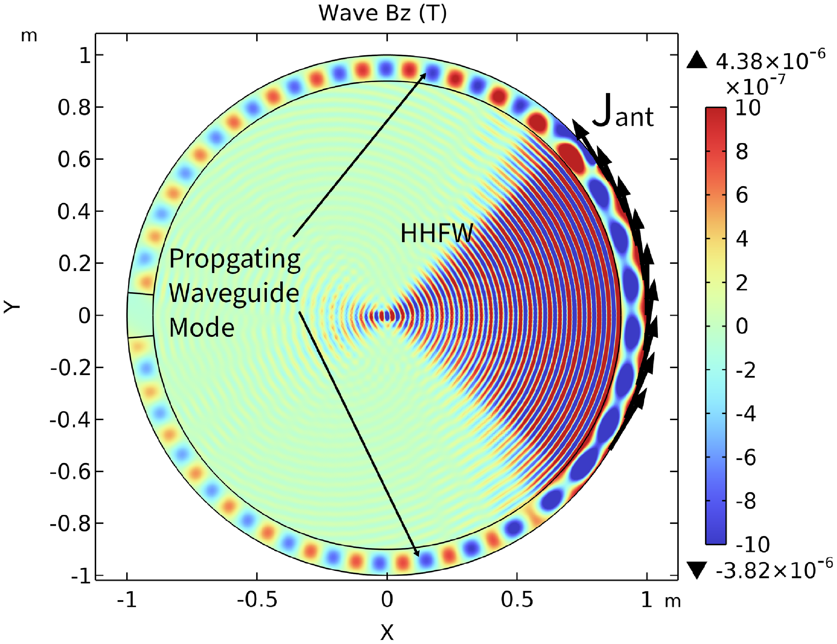
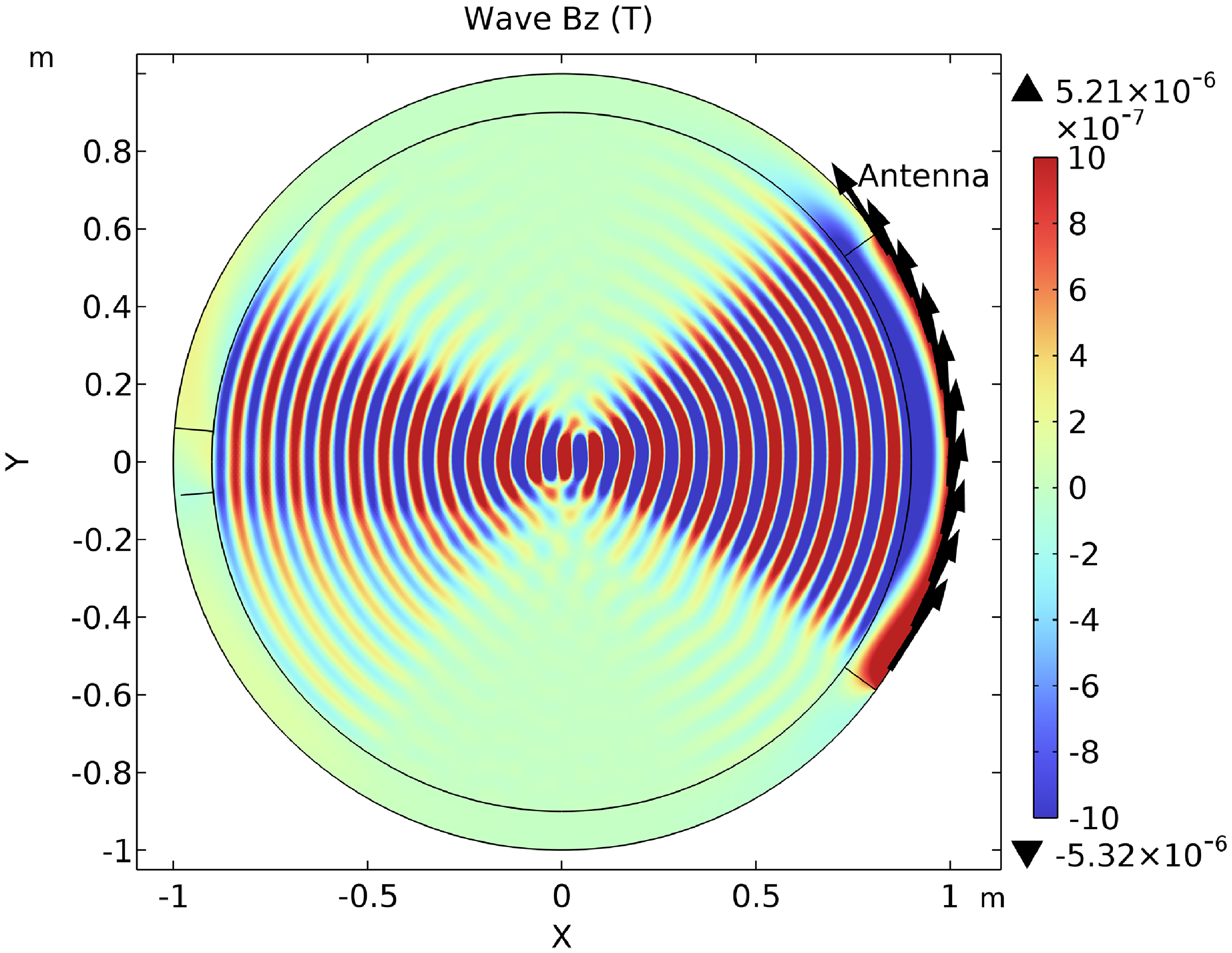
Figure 1 presents a 2-D circular model constructed based on NSTX parameters. The plasma is assumed to consist of electrons and a single ion species (deuterium). The geometry is infinite in the axial (z-) direction, and the plane wave variation ( $\exp (-ik_zz)$
) is assumed in that axial direction. The axial wave wavenumber (
$\exp (-ik_zz)$
) is assumed in that axial direction. The axial wave wavenumber ( $k_z$
) is an input parameter. Only the uniform axial background magnetic field,
$k_z$
) is an input parameter. Only the uniform axial background magnetic field, $B_{z}$
= 0.4 T, is considered in this section (
$B_{z}$
= 0.4 T, is considered in this section ( $k_\parallel = k_z$
), which will be adjusted in §§ 3 and 4. The core plasma has a constant density of
$k_\parallel = k_z$
), which will be adjusted in §§ 3 and 4. The core plasma has a constant density of $n_{e,core}$
=
$n_{e,core}$
= $3\times 10^{19}\, \mathrm{m}^{-3}$
, while the outer annular SOL density is reduced to
$3\times 10^{19}\, \mathrm{m}^{-3}$
, while the outer annular SOL density is reduced to $n_{e,SOL}$
=
$n_{e,SOL}$
= $3\times 10^{18}\, \mathrm{m}^{-3}$
. The SOL density chosen is sufficiently high to allow a propagating wave solution above the R-cutoff density for a wide range of
$3\times 10^{18}\, \mathrm{m}^{-3}$
. The SOL density chosen is sufficiently high to allow a propagating wave solution above the R-cutoff density for a wide range of $k_{\parallel }$
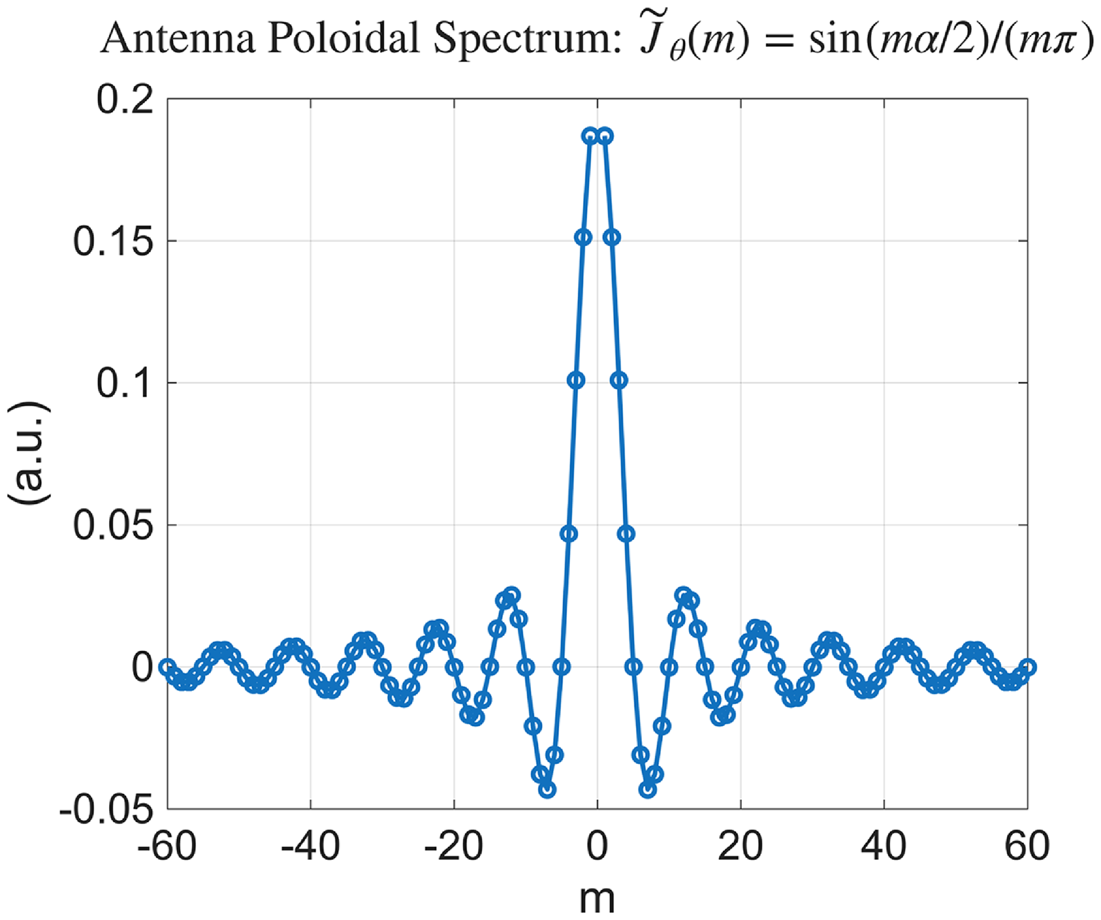
in order to isolate the geometric constraint. (The HHFW dispersion is shown in figure 5.) The density magnitude and its step-like profile are a simple adoption of the NSTX 130608 density profile. The annular SOL has a width of 0.1 m, representing a nominal distance from the last closed flux surface (LCFS) and antenna on NSTX. The core plasma radius is 0.9 m. In this geometry, the antenna is located at r = 1.0 m on a finite azimuthal arc from
$k_{\parallel }$
in order to isolate the geometric constraint. (The HHFW dispersion is shown in figure 5.) The density magnitude and its step-like profile are a simple adoption of the NSTX 130608 density profile. The annular SOL has a width of 0.1 m, representing a nominal distance from the last closed flux surface (LCFS) and antenna on NSTX. The core plasma radius is 0.9 m. In this geometry, the antenna is located at r = 1.0 m on a finite azimuthal arc from $\theta = -36^{\circ }$
to
$\theta = -36^{\circ }$
to $\theta = +36^{\circ }$
at the right-hand side (‘low-field side’) of the model, which produces a tangent current of
$\theta = +36^{\circ }$
at the right-hand side (‘low-field side’) of the model, which produces a tangent current of $\boldsymbol{J}_{\!{ant}} = -\sin \theta \, \hat {x}+\cos \theta \, \hat {y}$
. This antenna excites a spectrum of azimuthal modes (m =
$\boldsymbol{J}_{\!{ant}} = -\sin \theta \, \hat {x}+\cos \theta \, \hat {y}$
. This antenna excites a spectrum of azimuthal modes (m = $k_{\theta } r$
) at
$k_{\theta } r$
) at $f_0$
= 30 MHz, whose amplitude dependence follows a sinc-type function, as shown in figure 2. The full width of the main lobe is 4
$f_0$
= 30 MHz, whose amplitude dependence follows a sinc-type function, as shown in figure 2. The full width of the main lobe is 4 $\pi /\alpha$
, where
$\pi /\alpha$
, where $\alpha$
is the antenna arc angle in radians. As pointed out in the annulus resonance study (Perkins et al. Reference Perkins, Hosea, Bertelli, Taylor and Wilson2016), high-m modes can be selectively coupled and amplified by the SOL resonance condition, and can be a major contributor to the wavefield in the SOL. Since the SOL annular width remains the same outside the antenna azimuthal extent, these resonant poloidal modes are also responsible for the waveguide mode with slightly modified boundary conditions because the outer-wall boundary is changed from the antenna boundary to a perfect electric conductor (PEC), as will be discussed below.
$\alpha$
is the antenna arc angle in radians. As pointed out in the annulus resonance study (Perkins et al. Reference Perkins, Hosea, Bertelli, Taylor and Wilson2016), high-m modes can be selectively coupled and amplified by the SOL resonance condition, and can be a major contributor to the wavefield in the SOL. Since the SOL annular width remains the same outside the antenna azimuthal extent, these resonant poloidal modes are also responsible for the waveguide mode with slightly modified boundary conditions because the outer-wall boundary is changed from the antenna boundary to a perfect electric conductor (PEC), as will be discussed below.
Azimuthal spectrum of a circular-arc-shaped antenna with an angular extent of $\alpha$
= 72
$\alpha$
= 72 $^\circ$
:
$^\circ$
: $\tilde {J}_\theta (m) = \sin (m\alpha /2)/(m\pi )$
, where m is the azimuthal mode number. In the
$\tilde {J}_\theta (m) = \sin (m\alpha /2)/(m\pi )$
, where m is the azimuthal mode number. In the $m \rightarrow$
0 limit,
$m \rightarrow$
0 limit, $\tilde {J}_\theta = \alpha /(2\pi )$
.
$\tilde {J}_\theta = \alpha /(2\pi )$
.
In addition to the HHFW wavefield in the plasma core, figure 1 shows the wavefield structure localised in the annular SOL, propagating azimuthally within that region. In the upper part of the antenna region, the poloidal phase front propagates counterclockwise, while in the lower part it propagates clockwise. The input axial wavenumber is $k_z = k_{\parallel } = 3\,\mathrm{m}^{-1}$
. With the antenna exciting a tangential current, the wavefield excited is dominantly the transverse electric (TE) mode, with a large azimuthal electric field
$k_z = k_{\parallel } = 3\,\mathrm{m}^{-1}$
. With the antenna exciting a tangential current, the wavefield excited is dominantly the transverse electric (TE) mode, with a large azimuthal electric field $E_\theta$
and axial magnetic field (
$E_\theta$
and axial magnetic field ( $B_z$
). In the low density, particularly just above the R-cutoff density, the dominant power-flow direction can be axial (parallel to B), in line with the fast-wave dispersion (Hosea et al. Reference Hosea2008). In the core, the standard fast-wave propagation is visible. The uniform conductive loss is intentionally introduced in the plasma core (
$B_z$
). In the low density, particularly just above the R-cutoff density, the dominant power-flow direction can be axial (parallel to B), in line with the fast-wave dispersion (Hosea et al. Reference Hosea2008). In the core, the standard fast-wave propagation is visible. The uniform conductive loss is intentionally introduced in the plasma core ( $\sigma$
= 0.02) to minimise the wave interference and cavity effects. This effectively simulates a high single-pass absorption scenario. In the annular SOL, a small region is introduced at the opposite side of the antenna (
$\sigma$
= 0.02) to minimise the wave interference and cavity effects. This effectively simulates a high single-pass absorption scenario. In the annular SOL, a small region is introduced at the opposite side of the antenna ( $175^{\circ } \leqslant \theta \leqslant 185^{\circ }$
) with a high level of conduction loss (
$175^{\circ } \leqslant \theta \leqslant 185^{\circ }$
) with a high level of conduction loss ( $\sigma$
= 1) as a sink region to prevent wave interferences between the two propagating SOL modes.
$\sigma$
= 1) as a sink region to prevent wave interferences between the two propagating SOL modes.
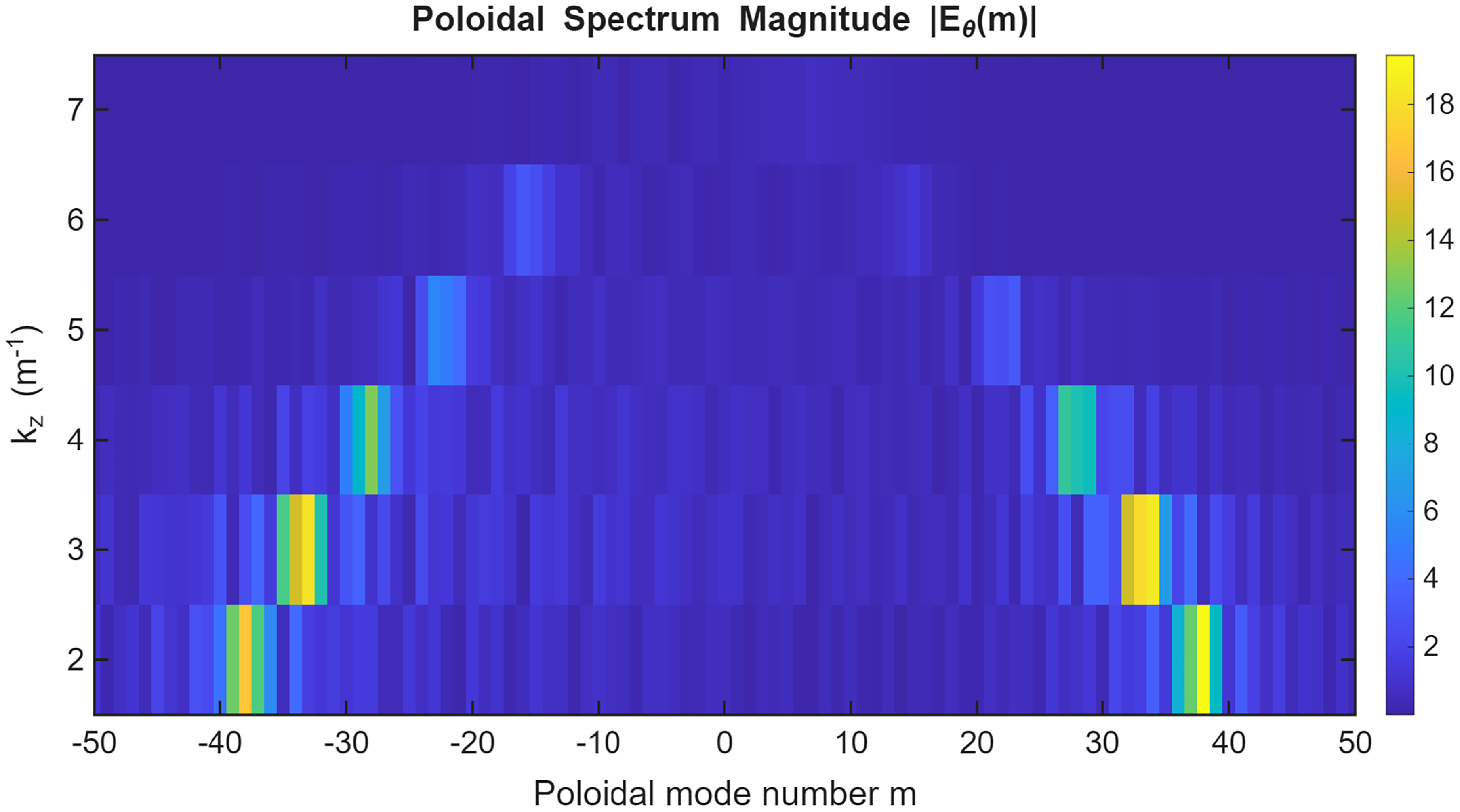
Poloidal spectrum of the wave $E_\theta$
along the circumference at r = 0.95 m in the middle of the annular SOL at different input
$E_\theta$
along the circumference at r = 0.95 m in the middle of the annular SOL at different input $k_\parallel$
.
$k_\parallel$
.
2.2. Impact of $k_\parallel$
on SOL waveguide mode
$k_\parallel$
on SOL waveguide mode

The input $k_z=k_\parallel$
plays an important role in generating the SOL waveguide mode by governing the wave perpendicular wavelength. To identify the corresponding azimuthal mode number of the propagating SOL mode at each
$k_z=k_\parallel$
plays an important role in generating the SOL waveguide mode by governing the wave perpendicular wavelength. To identify the corresponding azimuthal mode number of the propagating SOL mode at each $k_\parallel$
, figure 3 shows the poloidal mode spectrum of the theta component of the wave electric field (
$k_\parallel$
, figure 3 shows the poloidal mode spectrum of the theta component of the wave electric field ( ${E}_{\theta }$
) measured along the circumference at r = 0.95 m, located in the middle of the annular SOL between the core/SOL interface (r = 0.9 m) and the outer-wall boundary (r = 1 m). The input
${E}_{\theta }$
) measured along the circumference at r = 0.95 m, located in the middle of the annular SOL between the core/SOL interface (r = 0.9 m) and the outer-wall boundary (r = 1 m). The input $k_\parallel$
is varied from 2 to 7
$k_\parallel$
is varied from 2 to 7 $\mathrm{m}^{-1}$
. Both positive and negative azimuthal mode numbers
$\mathrm{m}^{-1}$
. Both positive and negative azimuthal mode numbers $m = k_\theta r$
are found, consistent with two oppositely propagating structures in figure 1. As
$m = k_\theta r$
are found, consistent with two oppositely propagating structures in figure 1. As $k_\parallel$
increases, however, the dominant azimuthal mode number (|m|) decreases, and no clear mode is observed for
$k_\parallel$
increases, however, the dominant azimuthal mode number (|m|) decreases, and no clear mode is observed for $k_{\parallel } \simeq 7\,\text{m}^{-1}$
. The corresponding mode amplitude decreases to zero, indicating no waveguide mode is supported at a high
$k_{\parallel } \simeq 7\,\text{m}^{-1}$
. The corresponding mode amplitude decreases to zero, indicating no waveguide mode is supported at a high $k_{\parallel }$
.
$k_{\parallel }$
.
Comparison between the peak poloidal mode numbers obtained from numerical modelling ( $m_{peak}$
) and the analytic estimates (
$m_{peak}$
) and the analytic estimates ( $m_{estimated}$
) as a function of
$m_{estimated}$
) as a function of $k_{\parallel } = k_z$
.
$k_{\parallel } = k_z$
.
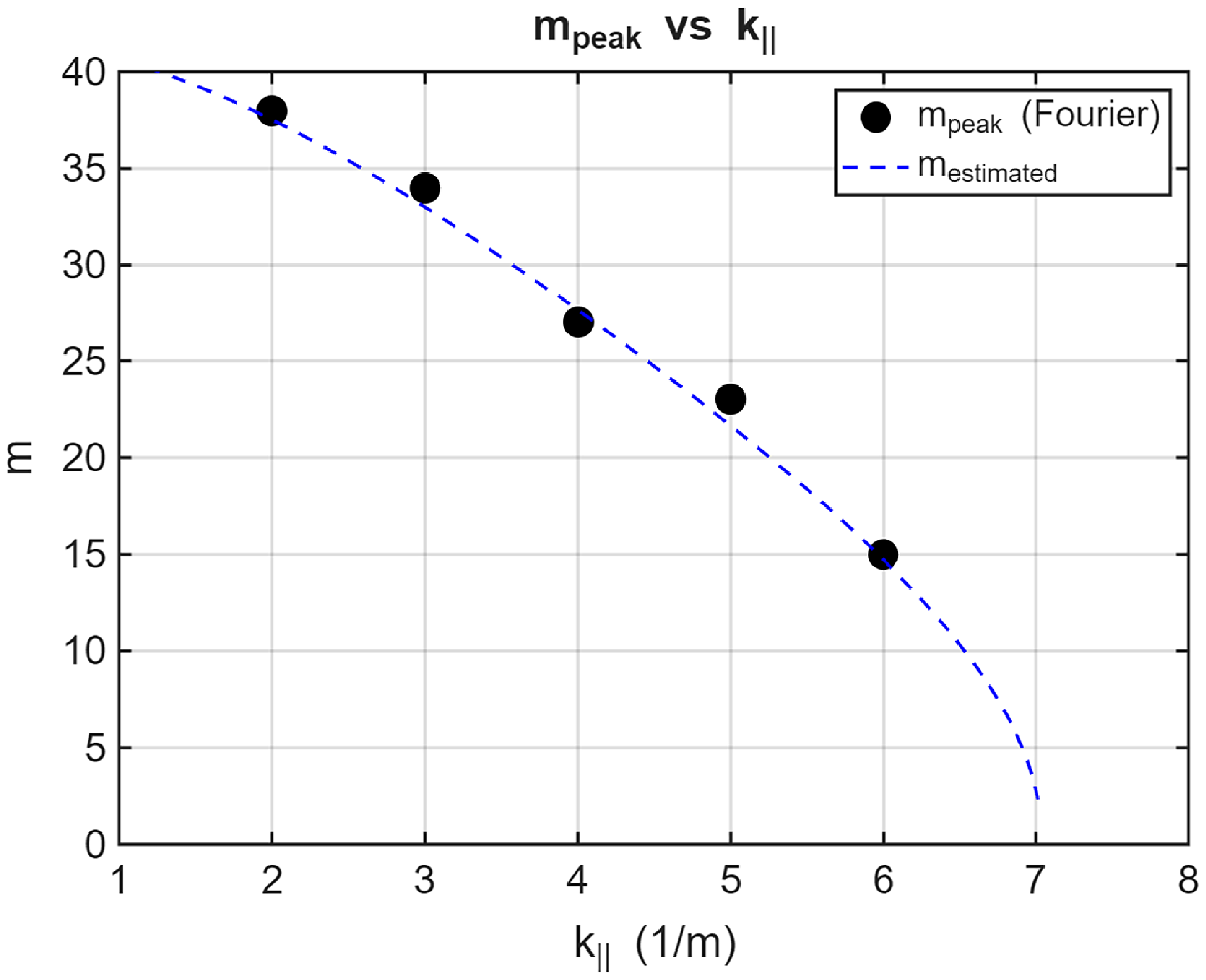
Figure 4 shows that the numerically observed azimuthal mode numbers agree with the analytical estimates based on the radial half-wavelength condition. The perpendicular wavenumber consists of the radial and azimuthal terms: $k_\perp ^2 = k_\theta ^2 + k_r^2$
. In the analysis,
$k_\perp ^2 = k_\theta ^2 + k_r^2$
. In the analysis, $k_r = \pi /\varDelta$
is imposed as a radial eigenmode constraint. At the same time, the poloidal mode number respects the HHFW dispersion relation, and
$k_r = \pi /\varDelta$
is imposed as a radial eigenmode constraint. At the same time, the poloidal mode number respects the HHFW dispersion relation, and $m_{estimated}$
is found
$m_{estimated}$
is found
 \begin{equation} m_{est} = r \sqrt {k_\perp ^2-(\pi /\varDelta )^2}, \end{equation}
where $k_\perp = (\omega /c)n_\perp$
can be found from the HHFW dispersion relation
$k_\perp = (\omega /c)n_\perp$
can be found from the HHFW dispersion relation
 \begin{equation} n_\perp ^2 = \frac {(n_{\parallel }^2-R)(n_{\parallel }^2-L)}{S-n_{\parallel }^2}, \end{equation}
where $L = 1 - {\sum}_j ({\omega _{pj}^2}/{(\omega (\omega - \varOmega _{cj}))})$
and
$L = 1 - {\sum}_j ({\omega _{pj}^2}/{(\omega (\omega - \varOmega _{cj}))})$
and $S = 1 - {\sum}_{j} ({\omega _{pj}^2}/{(\omega ^2 - \varOmega _{cj}^2)})$
.
$S = 1 - {\sum}_{j} ({\omega _{pj}^2}/{(\omega ^2 - \varOmega _{cj}^2)})$
.
The HHFW dispersion that shows the wave $k_\perp$
as a function of density for a given
$k_\perp$
as a function of density for a given $k_\parallel$
at
$k_\parallel$
at $B$
= 0.4 T and
$B$
= 0.4 T and $f_0$
= 30 MHz. Two horizontal lines represent the two perpendicular wavenumbers that provide half-wavelength (
$f_0$
= 30 MHz. Two horizontal lines represent the two perpendicular wavenumbers that provide half-wavelength ( $\lambda _\perp /2$
= 0.1 m) and quarter-wavelength (
$\lambda _\perp /2$
= 0.1 m) and quarter-wavelength ( $\lambda _\perp /2$
= 0.2 m) fits, respectively, for the SOL gap of 0.1 m at
$\lambda _\perp /2$
= 0.2 m) fits, respectively, for the SOL gap of 0.1 m at $n_e = 3\times 10^{18}\,\mathrm{m}^{-1}$
. For the case considered here,
$n_e = 3\times 10^{18}\,\mathrm{m}^{-1}$
. For the case considered here, $k_\parallel = 7$
and 13
$k_\parallel = 7$
and 13 $\mathrm{m}^{-1}$
meet the respective conditions.
$\mathrm{m}^{-1}$
meet the respective conditions.
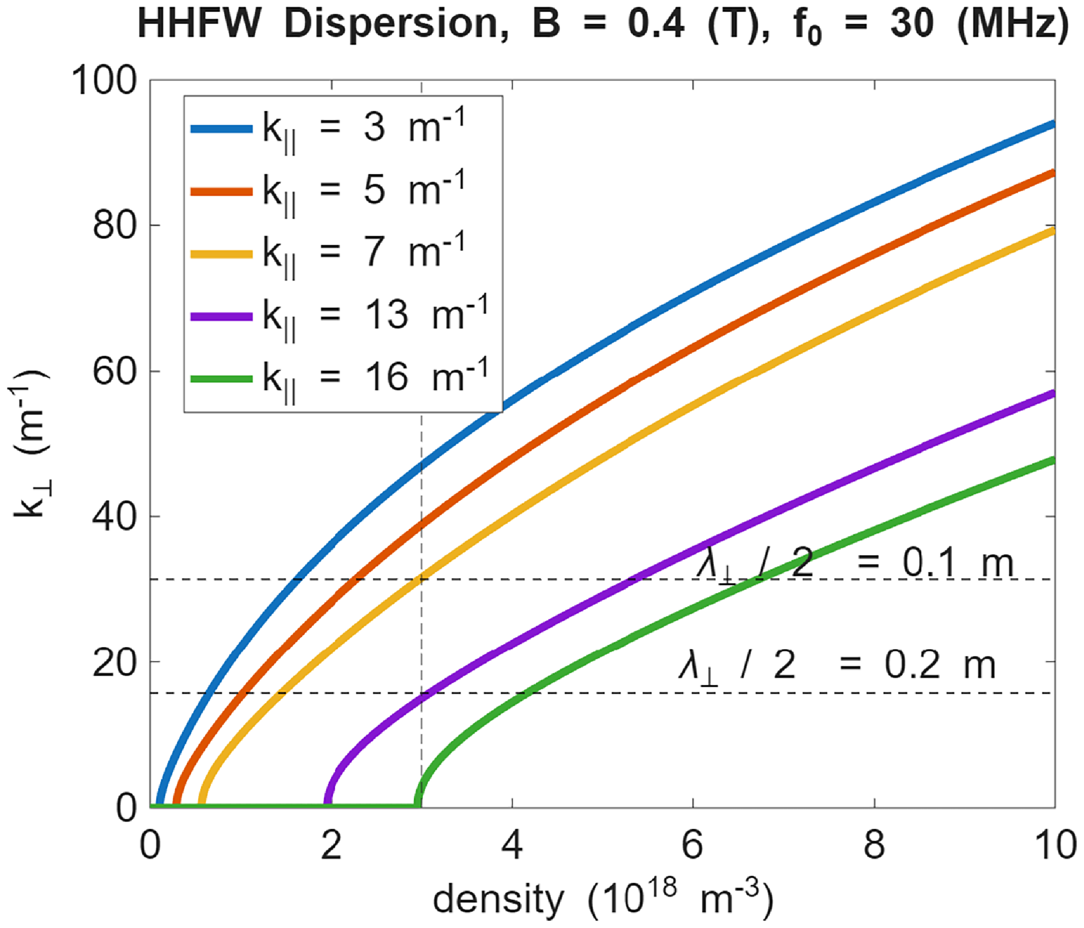
Figure 5 shows the corresponding $k_\perp$
values for various input wave
$k_\perp$
values for various input wave $k_{\parallel }$
. Note that, in the HHFW regime, the dispersion relation can be approximated to be
$k_{\parallel }$
. Note that, in the HHFW regime, the dispersion relation can be approximated to be $\omega \approx k_\perp v_A \sqrt (1+c^2k_{\parallel }^2/\omega _{pi}^2)$
, where
$\omega \approx k_\perp v_A \sqrt (1+c^2k_{\parallel }^2/\omega _{pi}^2)$
, where $v_A = B/\sqrt {\mu _0n_im_i}$
is the Alfvén speed. Increasing the wave
$v_A = B/\sqrt {\mu _0n_im_i}$
is the Alfvén speed. Increasing the wave $k_{\parallel }$
decreases
$k_{\parallel }$
decreases $k_\perp$
, and therefore limits the available azimuthal mode numbers since the radial wavenumber is constrained to be
$k_\perp$
, and therefore limits the available azimuthal mode numbers since the radial wavenumber is constrained to be $k_r = \pi /\varDelta$
, regardless of
$k_r = \pi /\varDelta$
, regardless of $k_{\parallel }$
. As shown in figure 4, the predictions from the dispersion relation agree well with the mode numbers found in the numerical modelling. Above
$k_{\parallel }$
. As shown in figure 4, the predictions from the dispersion relation agree well with the mode numbers found in the numerical modelling. Above $k_{\parallel } \approx 7\, \mathrm{m}^{-1}$
, no propagating waveguide mode can be supported because the HHFW perpendicular wavelength becomes too long to satisfy the half-wavelength condition. This cutoff mechanism is to be distinguished from the homogeneous fast-wave density R-cutoff condition, for which
$k_{\parallel } \approx 7\, \mathrm{m}^{-1}$
, no propagating waveguide mode can be supported because the HHFW perpendicular wavelength becomes too long to satisfy the half-wavelength condition. This cutoff mechanism is to be distinguished from the homogeneous fast-wave density R-cutoff condition, for which $n_\perp ^2 \lt 0$
. For the given SOL plasma, the R-cutoff occurs at
$n_\perp ^2 \lt 0$
. For the given SOL plasma, the R-cutoff occurs at $k_{\parallel } \gt 17\, \mathrm{m}^{-1}$
, well above the geometric cutoff.
$k_{\parallel } \gt 17\, \mathrm{m}^{-1}$
, well above the geometric cutoff.
2.3. Analysis of azimuthal mode-number structure
In this subsection, the azimuthal mode-number analysis is continued for $k_\parallel$
= 3 and
$k_\parallel$
= 3 and $7\,\mathrm{m}^{-1}$
. In addition to the Fourier transform analysis, another practical approach to identify the azimuthal mode number responsible for the radially standing-wave structure is to conduct a numerical mode-number analysis by applying the azimuthal phase factor,
$7\,\mathrm{m}^{-1}$
. In addition to the Fourier transform analysis, another practical approach to identify the azimuthal mode number responsible for the radially standing-wave structure is to conduct a numerical mode-number analysis by applying the azimuthal phase factor, $\exp (-i m_0 \theta )$
, to the antenna tangential current density
$\exp (-i m_0 \theta )$
, to the antenna tangential current density
 \begin{equation} \boldsymbol{J}_{\!{ant}} (m_0) =[-\sin \theta \hat {x}+\cos \theta \hat {y}]\exp (-im_0\theta ), \end{equation}
which will shift the centre of the antenna spectrum, and dominantly excite the $m_0\hbox{}$
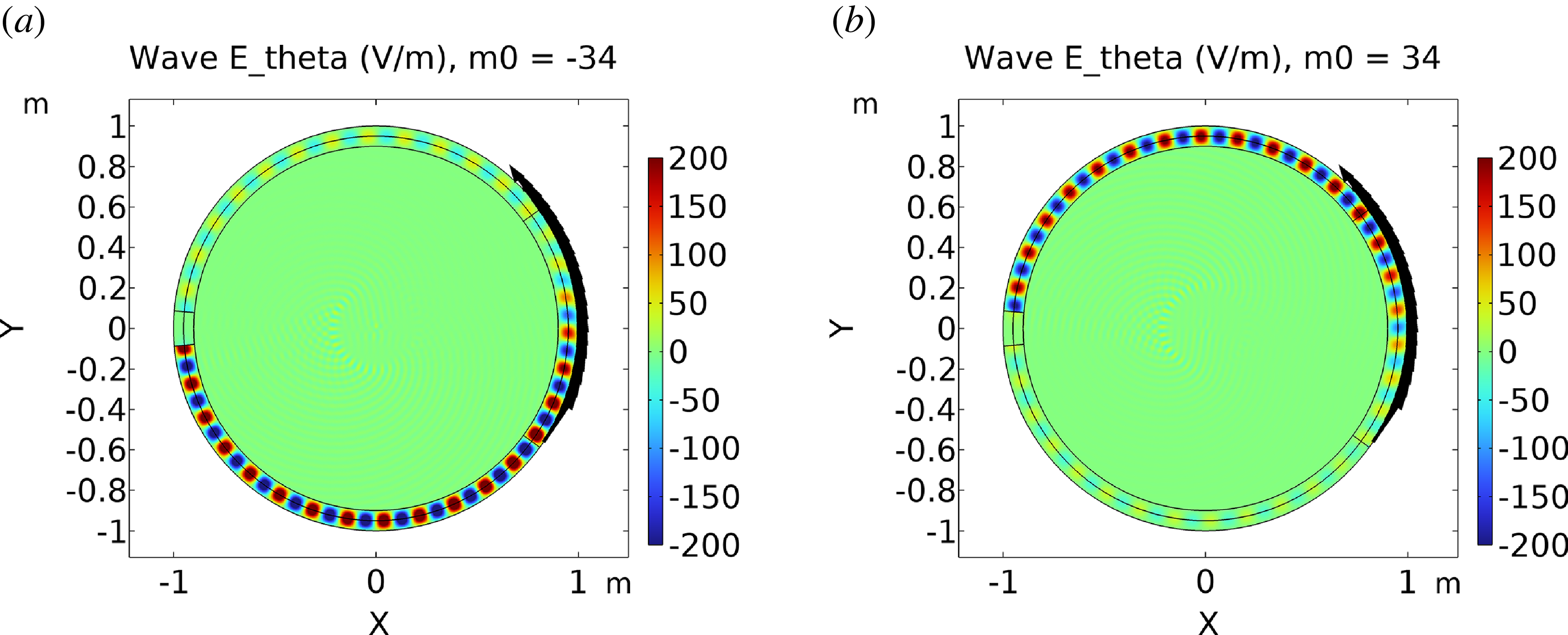
th harmonic Fourier mode. Figure 6 shows an example of the resulting wave
$m_0\hbox{}$
th harmonic Fourier mode. Figure 6 shows an example of the resulting wave $E_\theta$
for
$E_\theta$
for $\boldsymbol{J}_{\!{ant}} (m_0 = \pm 34)$
at
$\boldsymbol{J}_{\!{ant}} (m_0 = \pm 34)$
at $k_\parallel = 3\,\mathrm{m}^{-1}$
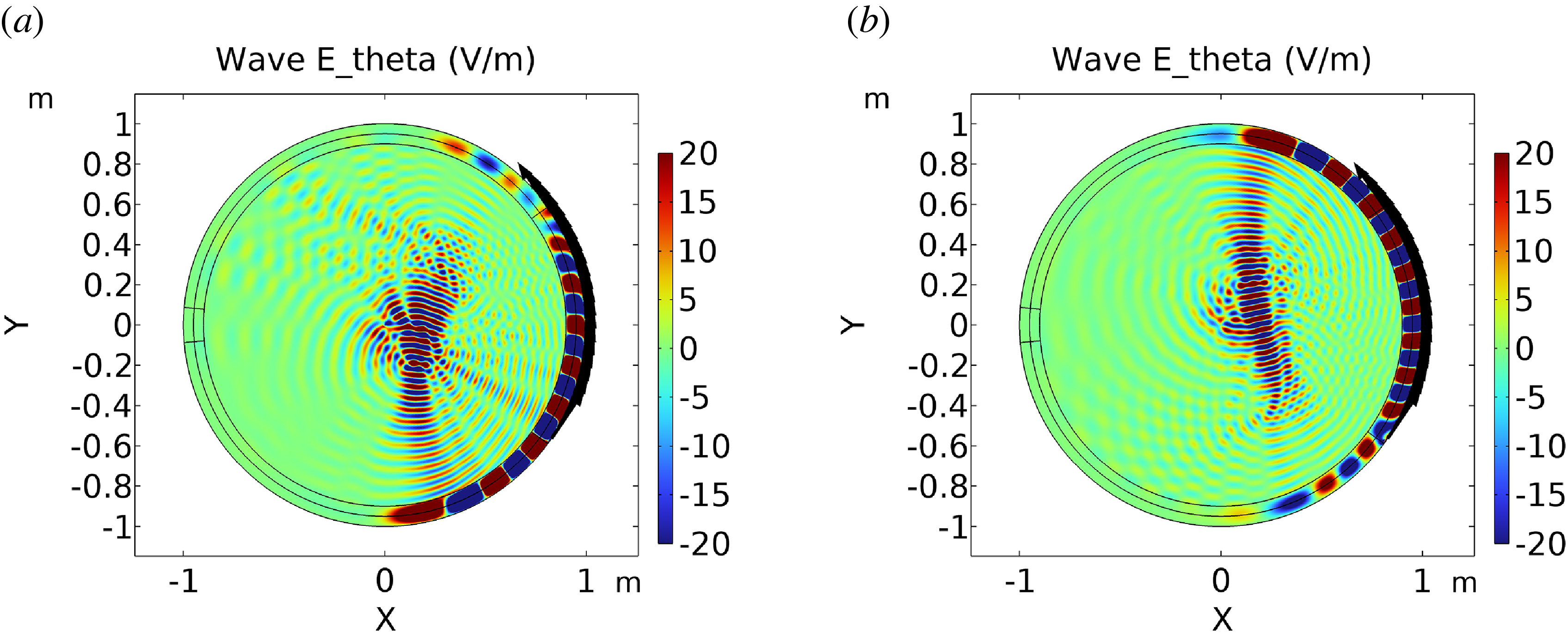
. The antenna power coupled is dominantly trapped in the SOL in both cases. A radially standing wavefield is formed in front of the antenna and propagates azimuthally, clockwise for
$k_\parallel = 3\,\mathrm{m}^{-1}$
. The antenna power coupled is dominantly trapped in the SOL in both cases. A radially standing wavefield is formed in front of the antenna and propagates azimuthally, clockwise for $m_0=-34$
and counterclockwise for
$m_0=-34$
and counterclockwise for $m_0=+34$
.
$m_0=+34$
.
The response of the wave tangential electric field ( $E_\theta$
) to the antenna current source:
$E_\theta$
) to the antenna current source: $\boldsymbol{j}_\theta =\hat {\theta } \mathrm{exp}(im_0\theta )$
, where
$\boldsymbol{j}_\theta =\hat {\theta } \mathrm{exp}(im_0\theta )$
, where $\hat {\theta }=-\mathrm{sin}\theta \,\hat {x}+\mathrm{cos}\theta \,\hat {y}$
, for (a)
$\hat {\theta }=-\mathrm{sin}\theta \,\hat {x}+\mathrm{cos}\theta \,\hat {y}$
, for (a) $m_0$
= –34 and (b)
$m_0$
= –34 and (b) $m_0$
= +34. The antenna azimuthal extent is indicated by a set of antenna current vectors. Here,
$m_0$
= +34. The antenna azimuthal extent is indicated by a set of antenna current vectors. Here, $k_z$
=
$k_z$
= $3\,\mathrm{m}^{-1}$
.
$3\,\mathrm{m}^{-1}$
.
At these resonant $m_0$
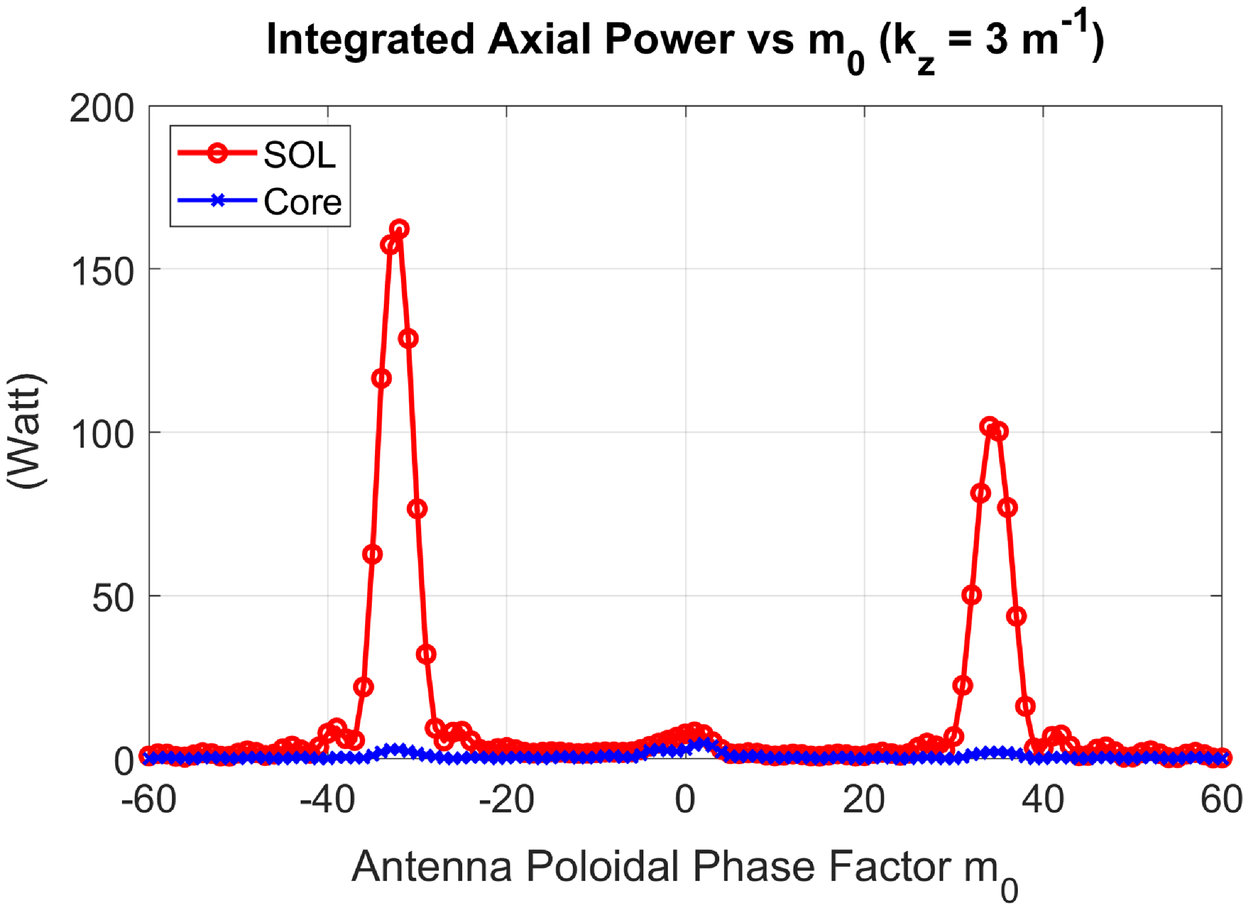
, the power coupled to the SOL is very high, indicating high antenna loading, while not necessarily meaning good core coupling (Hosea Reference Hosea2017). Here, ‘resonant’ refers to modes whose radial structure satisfies the half-wavelength condition in the SOL, leading to enhanced field amplitude and antenna loading. Figure 7 shows the area-integrated axial Poynting flux
$m_0$
, the power coupled to the SOL is very high, indicating high antenna loading, while not necessarily meaning good core coupling (Hosea Reference Hosea2017). Here, ‘resonant’ refers to modes whose radial structure satisfies the half-wavelength condition in the SOL, leading to enhanced field amplitude and antenna loading. Figure 7 shows the area-integrated axial Poynting flux $S_z = (1/2) \int (E_x H_y^* - E_y H_x^*){\rm d}A$
in both the core and annular SOL regions as a function of
$S_z = (1/2) \int (E_x H_y^* - E_y H_x^*){\rm d}A$
in both the core and annular SOL regions as a function of $m_0$
. Here,
$m_0$
. Here, $S_z$
is used as a measure of power coupling for the given antenna current magnitude, which represents the degree of bare loading at each
$S_z$
is used as a measure of power coupling for the given antenna current magnitude, which represents the degree of bare loading at each $m_0$
. The power flowing to the annular SOL (red curve) is maximum at the resonant values
$m_0$
. The power flowing to the annular SOL (red curve) is maximum at the resonant values $m_0 = \pm 34$
, where it exceeds the nominal
$m_0 = \pm 34$
, where it exceeds the nominal $m_0 = 0$
case by an order of magnitude.
$m_0 = 0$
case by an order of magnitude.
Please note that, in the absence of explicit wave power dissipation physics in the present model, the area-integrated axial Poynting flux strictly represents wave power flow and antenna loading, rather than being a direct measure of absorbed power in the plasma, which is a limitation of the cold-plasma treatment employed in this study. For example, for a realistic antenna spectrum including symmetric $\pm k_{\parallel }$
components, this approach would cause the net axial power flow to cancel, even though finite power is coupled to and absorbed by the plasma. In the limit of large conductive loss in the model, Poynting flux would vanish as well. Another possible approach is to consider power absorption from the conductive loss implemented in our model, but the chosen parameter is phenomenological (constant conductive loss in the core and non-uniform conductive loss in the annular SOL (please see § 2.1)). Therefore, throughout the manuscript, the term ‘power coupling’ is used in a loose sense, since it is expected that the power-flow quantity is proportional to the absorbed power under appropriate absorption models. For example, those wave powers present in the SOL can serve as a proxy for SOL parasitic power absorptions in the experiment, as they are expected to drive a range of parasitic wave–edge interactions, such as collisions, sheath rectification (Perkins et al. Reference Perkins2012, Reference Perkins, Hosea, Jaworski, Bell, Bertelli, Kramer, Roquemore, Taylor and Wilson2017b
), filament-assisted mode conversion to slow waves (Tierens et al. Reference Tierens, Bilato, Bertelli, Shiraiwa, Myra and Colas2022) and parametric decay instabilities (Wilson et al. Reference Wilson, Bernabei, Biewer, Diem, Hosea, LeBlanc, Phillips, Ryan and Swain2005).
$\pm k_{\parallel }$
components, this approach would cause the net axial power flow to cancel, even though finite power is coupled to and absorbed by the plasma. In the limit of large conductive loss in the model, Poynting flux would vanish as well. Another possible approach is to consider power absorption from the conductive loss implemented in our model, but the chosen parameter is phenomenological (constant conductive loss in the core and non-uniform conductive loss in the annular SOL (please see § 2.1)). Therefore, throughout the manuscript, the term ‘power coupling’ is used in a loose sense, since it is expected that the power-flow quantity is proportional to the absorbed power under appropriate absorption models. For example, those wave powers present in the SOL can serve as a proxy for SOL parasitic power absorptions in the experiment, as they are expected to drive a range of parasitic wave–edge interactions, such as collisions, sheath rectification (Perkins et al. Reference Perkins2012, Reference Perkins, Hosea, Jaworski, Bell, Bertelli, Kramer, Roquemore, Taylor and Wilson2017b
), filament-assisted mode conversion to slow waves (Tierens et al. Reference Tierens, Bilato, Bertelli, Shiraiwa, Myra and Colas2022) and parametric decay instabilities (Wilson et al. Reference Wilson, Bernabei, Biewer, Diem, Hosea, LeBlanc, Phillips, Ryan and Swain2005).
Area-integrated axial Poynting flux $S_z = (1/2) \int (E_x H_y^* - E_y H_x^*){\rm d}A$
in both the core and annular SOL regions as a function of
$S_z = (1/2) \int (E_x H_y^* - E_y H_x^*){\rm d}A$
in both the core and annular SOL regions as a function of $m_0$
in the antenna current source. Here,
$m_0$
in the antenna current source. Here, $k_z$
=
$k_z$
= $3\,\mathrm{m}^{-1}$
and
$3\,\mathrm{m}^{-1}$
and $B$
= 0.4 T.
$B$
= 0.4 T.
Area integrated axial Poynting flux between the core and annular SOL regions as a function $k_{\parallel }$
, showing the dependence of antenna loading on
$k_{\parallel }$
, showing the dependence of antenna loading on $k_\parallel$
. The secondary x-axis shows the corresponding
$k_\parallel$
. The secondary x-axis shows the corresponding $(\lambda _{\perp }/2)/\varDelta$
.
$(\lambda _{\perp }/2)/\varDelta$
.
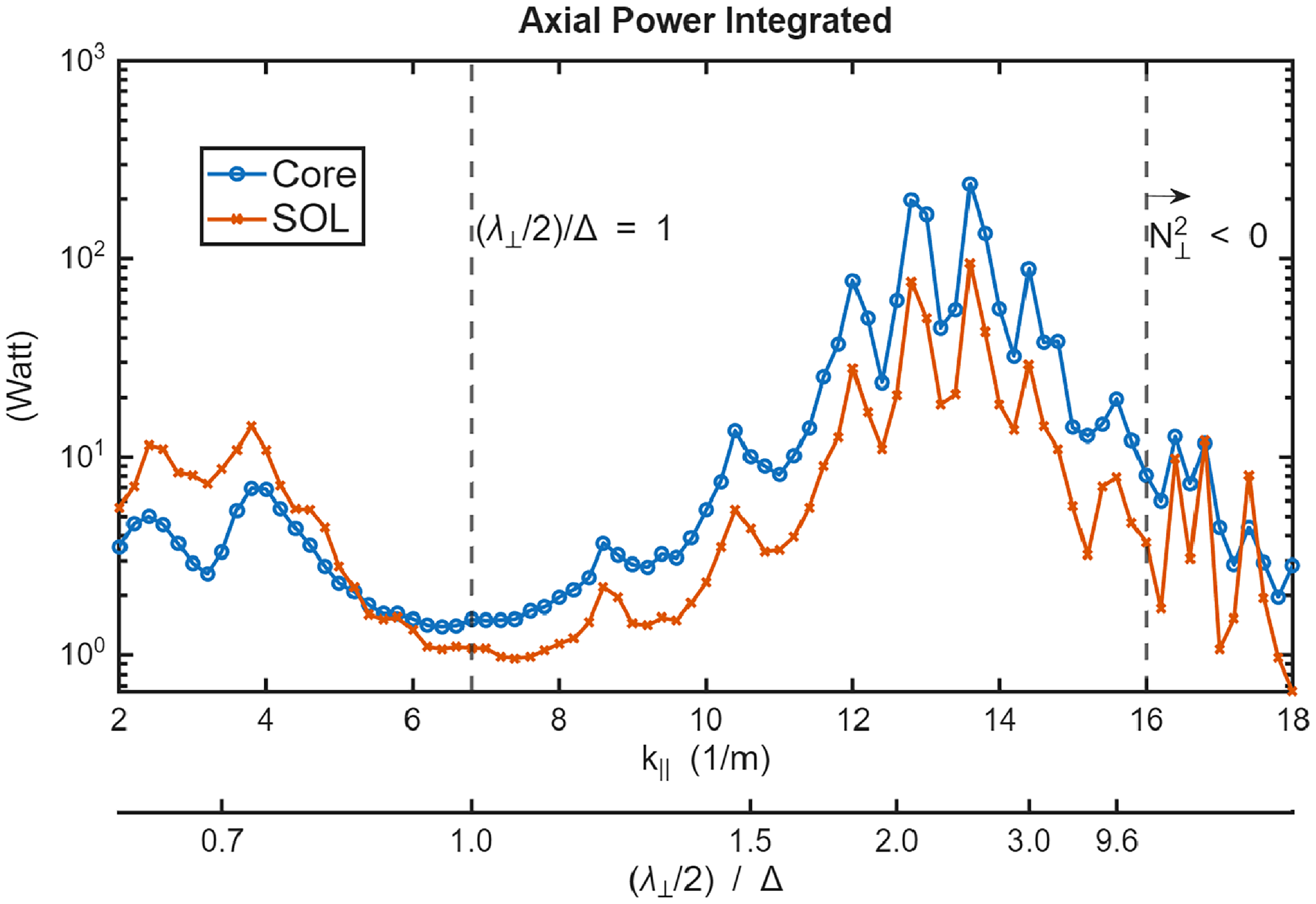
As shown in figure 8, when the half-wavelength condition is satisfied at low $k_\parallel$
, a substantial fraction of the coupled power is transported by the SOL waveguide mode. However, above
$k_\parallel$
, a substantial fraction of the coupled power is transported by the SOL waveguide mode. However, above $k_\parallel \approx 7\,\mathrm{m}^{-1}$
, the power coupled to the plasma core starts to exceed the power coupled to the annular SOL. At
$k_\parallel \approx 7\,\mathrm{m}^{-1}$
, the power coupled to the plasma core starts to exceed the power coupled to the annular SOL. At $k_\parallel \approx 13\,\mathrm{m}^{-1}$
, close to the quarter-wavelength condition as shown in the HHFW dispersion in figure 5, the total amount of power coupled into the plasma increases by an order of magnitude, reaching its maximum. This resonant dependence of the loading on
$k_\parallel \approx 13\,\mathrm{m}^{-1}$
, close to the quarter-wavelength condition as shown in the HHFW dispersion in figure 5, the total amount of power coupled into the plasma increases by an order of magnitude, reaching its maximum. This resonant dependence of the loading on $k_\parallel$
has implications for future experiments and will be explored in a separate work. Finally, when the fast-wave R-cutoff condition is not met above
$k_\parallel$
has implications for future experiments and will be explored in a separate work. Finally, when the fast-wave R-cutoff condition is not met above $k_\parallel = 16\,\mathrm{m}^{-1}$
, the loading is reduced.
$k_\parallel = 16\,\mathrm{m}^{-1}$
, the loading is reduced.
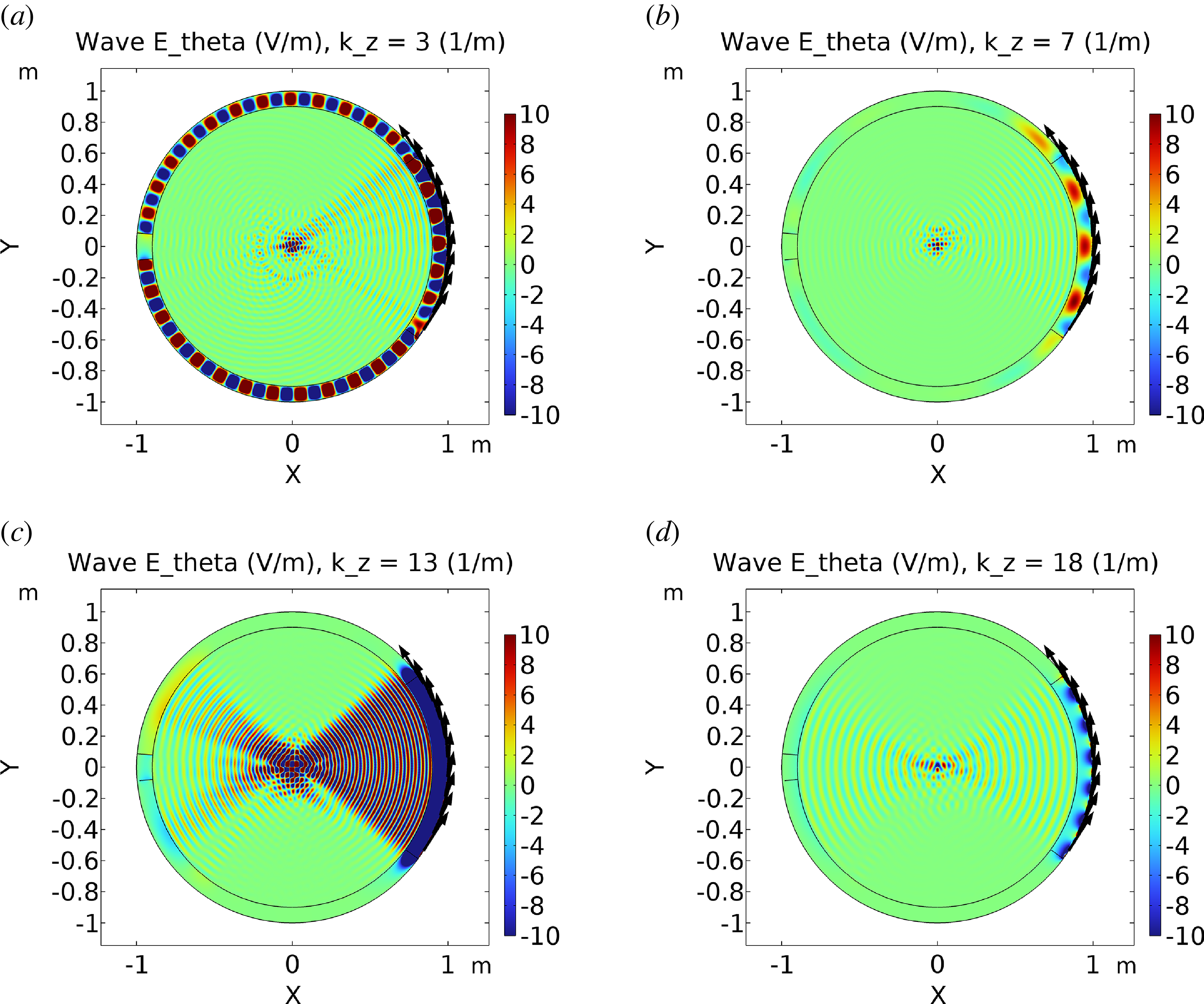
Figure 9 shows the corresponding wave $E_\theta$
at different
$E_\theta$
at different $k_\parallel =$
3, 7, 13 and 18
$k_\parallel =$
3, 7, 13 and 18 $\mathrm{m}^{-1}$
. In the figures, the colour bar range for the wave
$\mathrm{m}^{-1}$
. In the figures, the colour bar range for the wave $E_\theta$
is kept the same for visualisation purposes. At
$E_\theta$
is kept the same for visualisation purposes. At $k_{\parallel }$
= 3
$k_{\parallel }$
= 3 $\mathrm{m}^{-1}$
, the impact of resonant high-m components,
$\mathrm{m}^{-1}$
, the impact of resonant high-m components, $m\approx \pm 34$
, is apparent. Because the magnetic geometry is aligned with the model axial geometry, the azimuthal mode number supported by the SOL plasma
$m\approx \pm 34$
, is apparent. Because the magnetic geometry is aligned with the model axial geometry, the azimuthal mode number supported by the SOL plasma $m$
matches the input antenna phase factor
$m$
matches the input antenna phase factor $m_0$
. At
$m_0$
. At $k_z$
= 7
$k_z$
= 7 $\mathrm{m}^{-1}$
, the propagating SOL mode is no longer observed outside the antenna as the SOL cannot naturally support the radial eigenmode half-wavelength structure. At
$\mathrm{m}^{-1}$
, the propagating SOL mode is no longer observed outside the antenna as the SOL cannot naturally support the radial eigenmode half-wavelength structure. At $k_z$
= 13
$k_z$
= 13 $\mathrm{m}^{-1}$
, the azimuthal distribution of the wavefield within the antenna extent is nearly flat (
$\mathrm{m}^{-1}$
, the azimuthal distribution of the wavefield within the antenna extent is nearly flat ( $m\approx 0$
). Finally, a high-m surface-wave-like mode is observed at
$m\approx 0$
). Finally, a high-m surface-wave-like mode is observed at $k_{z} = 18\, \mathrm{m}^{-1}$
, and the overall power coupling to plasma is strongly reduced.
$k_{z} = 18\, \mathrm{m}^{-1}$
, and the overall power coupling to plasma is strongly reduced.
The $E_\theta$
profile at different
$E_\theta$
profile at different $k_z$
: (a) 3
$k_z$
: (a) 3 $\mathrm{m}^{-1}$
, (b) 7
$\mathrm{m}^{-1}$
, (b) 7 $\mathrm{m}^{-1}$
, (c) 13
$\mathrm{m}^{-1}$
, (c) 13 $\mathrm{m}^{-1}$
and (d) 18
$\mathrm{m}^{-1}$
and (d) 18 $\mathrm{m}^{-1}$
.
$\mathrm{m}^{-1}$
.
(a) Fractional SOL power to the total power (SOL + core) and (b) fractional annulus power outside the antenna extent to the total SOL power as a function of $k_\parallel$
.
$k_\parallel$
.
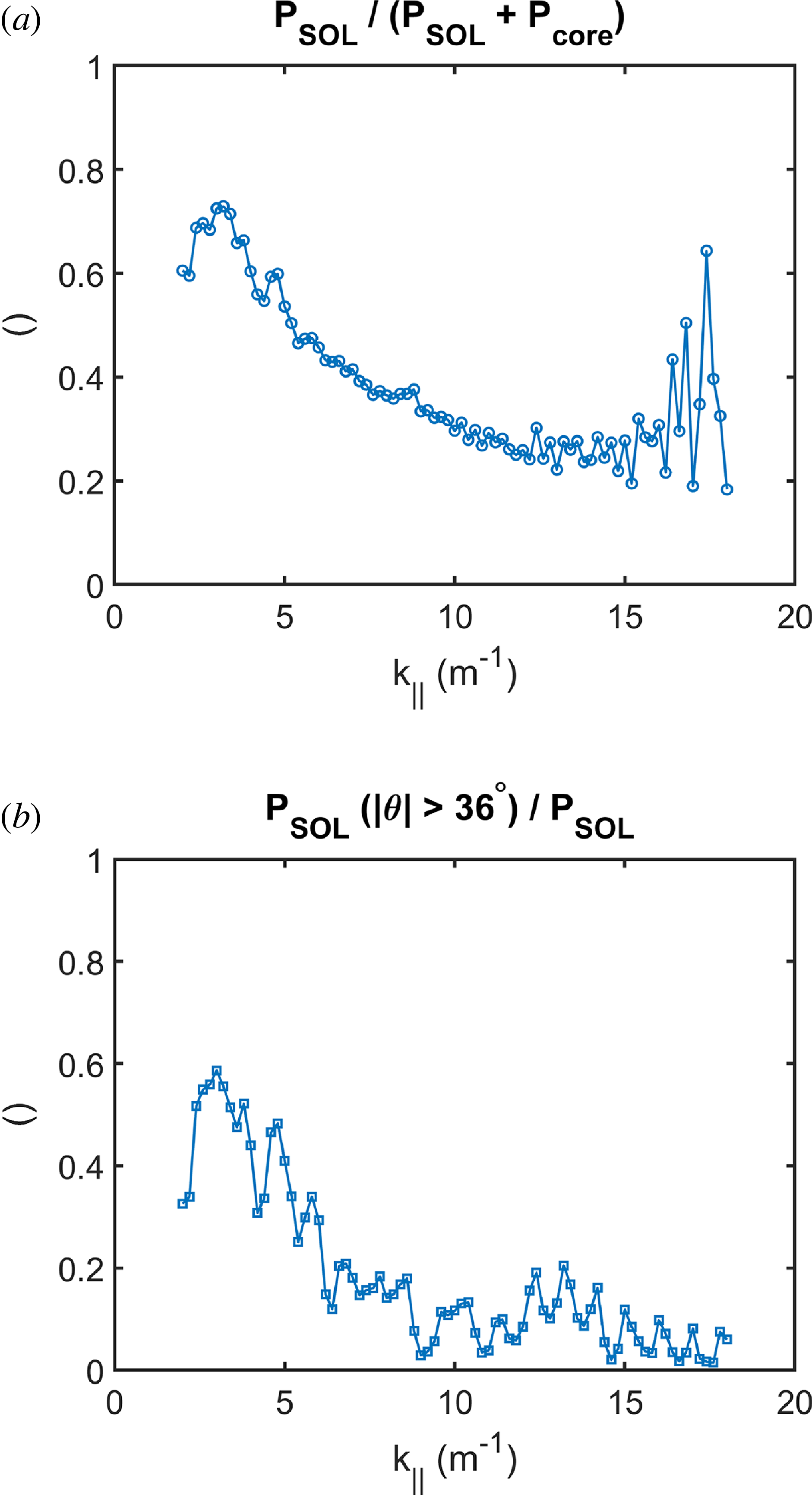
As shown in figure 10(a), the fractional power in the annular SOL ( $S_{z,SOL}$
) relative to the total power (
$S_{z,SOL}$
) relative to the total power ( $S_{z,SOL}+S_{z,core}$
) is more than
$S_{z,SOL}+S_{z,core}$
) is more than $50\,\%$
of the total power at a low
$50\,\%$
of the total power at a low $k_z \lt 5$ $\mathrm{m}^{-1}$
. Such a large fraction coupled to the SOL is consistent with the experimental trend that power loss is aggravated at low
$\mathrm{m}^{-1}$
. Such a large fraction coupled to the SOL is consistent with the experimental trend that power loss is aggravated at low $k_{\phi }$
. Furthermore, the power carried by the waveguide mode outside the antenna region can be non-negligible, as shown in figure 10(b). More than 50
$k_{\phi }$
. Furthermore, the power carried by the waveguide mode outside the antenna region can be non-negligible, as shown in figure 10(b). More than 50 $\%$
of the SOL power is accounted for by the propagating mode. This is due mainly to a longer extent of the annular SOL outside the antenna, as the antenna azimuthal extent spans only 20
$\%$
of the SOL power is accounted for by the propagating mode. This is due mainly to a longer extent of the annular SOL outside the antenna, as the antenna azimuthal extent spans only 20 $\%$
of the total circumference (
$\%$
of the total circumference ( $|\theta |\lt 36^{\circ }$
) in the model. The SOL mode is continuously supported in the annular SOL until it reaches the artificial sink region at the opposite side of the antenna. In real-world experiments, the magnetic and physical geometries should be taken into account, as discussed in later sections, and the details of these power fractions are expected to vary. Past modelling (Bertelli et al. Reference Bertelli2016) using the NSTX geometry has reported parasitic power losses of up to 40
$|\theta |\lt 36^{\circ }$
) in the model. The SOL mode is continuously supported in the annular SOL until it reaches the artificial sink region at the opposite side of the antenna. In real-world experiments, the magnetic and physical geometries should be taken into account, as discussed in later sections, and the details of these power fractions are expected to vary. Past modelling (Bertelli et al. Reference Bertelli2016) using the NSTX geometry has reported parasitic power losses of up to 40 $\%$
in the SOL, so these power fractions are not considered unreasonable.
$\%$
in the SOL, so these power fractions are not considered unreasonable.
As was shown in figure 9(b), the propagating SOL mode is no longer observed outside the antenna at $k_z$
= 7
$k_z$
= 7 $\mathrm{m}^{-1}$
. However, a poloidal structure is still observed in front of the antenna, which exhibits a higher mode-number structure than
$\mathrm{m}^{-1}$
. However, a poloidal structure is still observed in front of the antenna, which exhibits a higher mode-number structure than $m \approx 2$
from the analytic mode estimates in figure 4. Compared with the PEC boundary (
$m \approx 2$
from the analytic mode estimates in figure 4. Compared with the PEC boundary ( $E_\theta =0$
) at the outer wall for the SOL waveguide mode, the boundary condition is expected to be modified in the presence of the antenna current boundary, and can be generalised to
$E_\theta =0$
) at the outer wall for the SOL waveguide mode, the boundary condition is expected to be modified in the presence of the antenna current boundary, and can be generalised to
 \begin{align} E_\theta + Z\frac {{\rm d}E_\theta }{{\rm d}r}=0. \end{align}
This is as a general form of the boundary condition based on Ampere’s law that gives $H_z \propto {\rm d}E_\theta /{\rm d}r$
, as the tangential antenna current drives the wave
$H_z \propto {\rm d}E_\theta /{\rm d}r$
, as the tangential antenna current drives the wave $B_z$
from the surface boundary condition:
$B_z$
from the surface boundary condition: $\boldsymbol{n} \times (\boldsymbol{H}_{plasma}-\boldsymbol{H}_{wall})=J_\theta \hat {\theta }$
. In the PEC boundary, Z = 0, and the radial wavenumber condition in the annular SOL recovers the standard half-wavelength condition. With the antenna boundary, however, the antenna current may impose a specific phase shift to the wavefield, effectively reducing
$\boldsymbol{n} \times (\boldsymbol{H}_{plasma}-\boldsymbol{H}_{wall})=J_\theta \hat {\theta }$
. In the PEC boundary, Z = 0, and the radial wavenumber condition in the annular SOL recovers the standard half-wavelength condition. With the antenna boundary, however, the antenna current may impose a specific phase shift to the wavefield, effectively reducing $k_r$
less than
$k_r$
less than $\pi /\varDelta$
, thus availing a finite level of
$\pi /\varDelta$
, thus availing a finite level of $k_\theta$
to induce a poloidal structure. This driven mode is not naturally supported outside the antenna azimuthal extent, and is absent in this case. If a functional form of
$k_\theta$
to induce a poloidal structure. This driven mode is not naturally supported outside the antenna azimuthal extent, and is absent in this case. If a functional form of $E_\theta (\xi ) \,\sim$
sin(
$E_\theta (\xi ) \,\sim$
sin( $k_r\xi$
) is assumed in the annular SOL with
$k_r\xi$
) is assumed in the annular SOL with $E_\theta (\xi =0) = 0$
and
$E_\theta (\xi =0) = 0$
and $E_\theta (\xi =\varDelta ) + Z({{\rm d}E_\theta }/{{\rm d}r})(\xi =\varDelta )=0$
, this boundary condition leads to
$E_\theta (\xi =\varDelta ) + Z({{\rm d}E_\theta }/{{\rm d}r})(\xi =\varDelta )=0$
, this boundary condition leads to
 \begin{align} k_r \varDelta +\tan^{-1}(Zk_r)=n\pi , \end{align}
where n is a multiple of integers. Based on the observed half-wavelength fit structure in the annular SOL, $E_{\theta } (\xi =0) = 0$
is imposed at the core–SOL interface. It is analogous to a PEC boundary at the outer wall where the tangential electric field vanishes. Here,
$E_{\theta } (\xi =0) = 0$
is imposed at the core–SOL interface. It is analogous to a PEC boundary at the outer wall where the tangential electric field vanishes. Here, $\xi$
denotes the radial coordinate across the SOL region, where
$\xi$
denotes the radial coordinate across the SOL region, where $\xi$
= 0 corresponds to the core–SOL interface and
$\xi$
= 0 corresponds to the core–SOL interface and $\xi$
=
$\xi$
= $\varDelta$
corresponds to the outer edge of the SOL. The half-wavelength case, n = 1, becomes
$\varDelta$
corresponds to the outer edge of the SOL. The half-wavelength case, n = 1, becomes
 \begin{equation} k_r =\frac {\pi - \phi }{\varDelta }, \end{equation}
where $\phi = \tan^{-1}(Zk_r)$
is an antenna-introduced phase-shift factor with Z being an effective impedance (
$\phi = \tan^{-1}(Zk_r)$
is an antenna-introduced phase-shift factor with Z being an effective impedance ( $\propto E_\theta / H_z$
) at a surface impedance boundary. For
$\propto E_\theta / H_z$
) at a surface impedance boundary. For $k_{z}=7\,\mathrm{m}^{-1}$
, the poloidal mode number seen is
$k_{z}=7\,\mathrm{m}^{-1}$
, the poloidal mode number seen is $m\approx 17$
, which corresponds to
$m\approx 17$
, which corresponds to $k_r \approx 26.7\, \mathrm{m}^{-1}$
, which is less than the wave
$k_r \approx 26.7\, \mathrm{m}^{-1}$
, which is less than the wave $k_\perp = 31.6\,\mathrm{m}^{-1}$
. This gives
$k_\perp = 31.6\,\mathrm{m}^{-1}$
. This gives $Z = \tan(\pi -k_r \varDelta )/k_r = 0.02$
.
$Z = \tan(\pi -k_r \varDelta )/k_r = 0.02$
.
Area-integrated axial Poynting flux $S_z = (1/2) \int (E_x H_y^* - E_y H_x^*){\rm d}A$
in both the core and annular SOL regions as a function of
$S_z = (1/2) \int (E_x H_y^* - E_y H_x^*){\rm d}A$
in both the core and annular SOL regions as a function of $m_0$
in the antenna current source:
$m_0$
in the antenna current source: $\boldsymbol{j}_\theta =\hat {\theta } \mathrm{exp}(im_0\theta )$
, where
$\boldsymbol{j}_\theta =\hat {\theta } \mathrm{exp}(im_0\theta )$
, where $\hat {\theta }=-\mathrm{sin}\theta \hat {x}+\mathrm{cos}\theta \hat {y}$
. Here,
$\hat {\theta }=-\mathrm{sin}\theta \hat {x}+\mathrm{cos}\theta \hat {y}$
. Here, $k_z$
=
$k_z$
= $7\,\mathrm{m}^{-1}$
.
$7\,\mathrm{m}^{-1}$
.
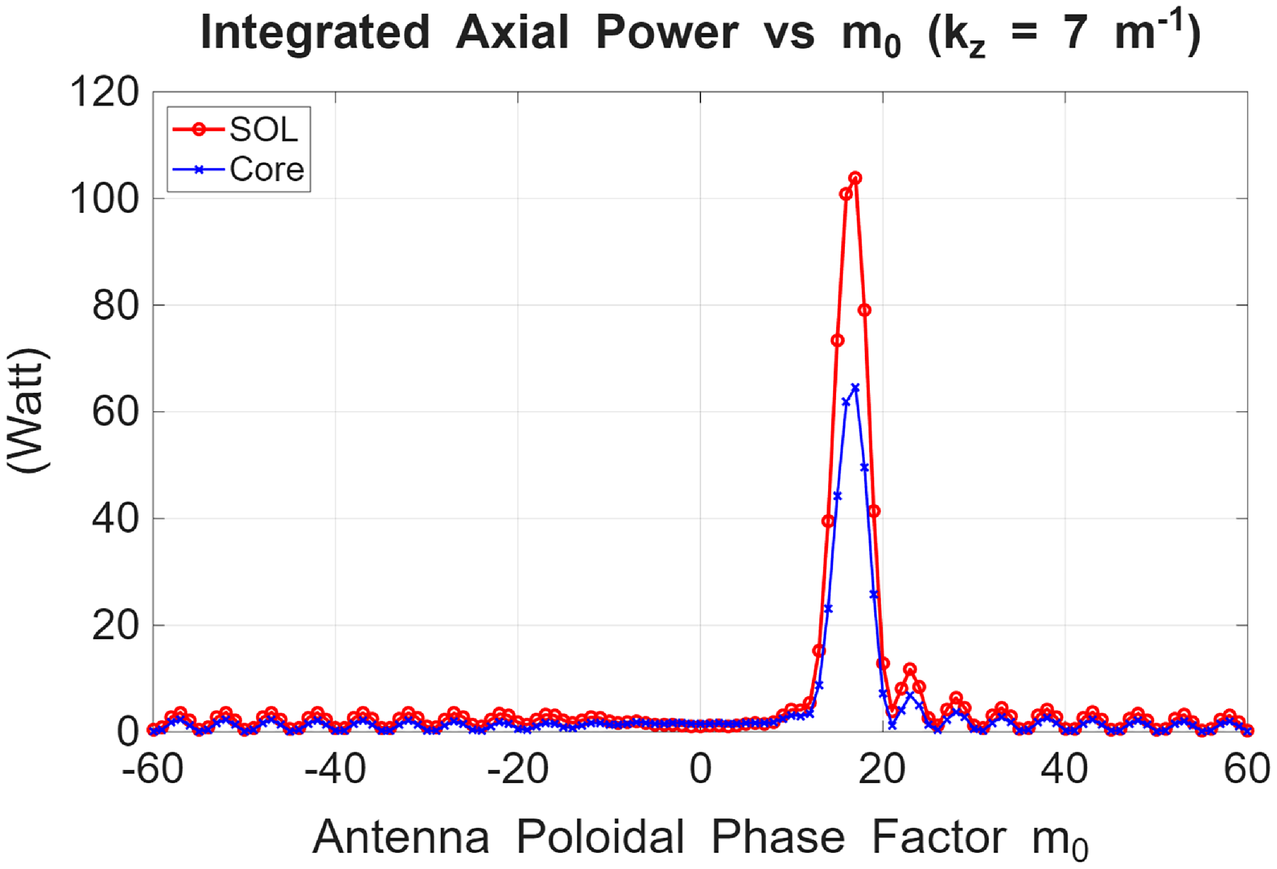
As shown in figure 11, the mode-number analysis is repeated for $k_z$
= 7
$k_z$
= 7 $\mathrm{m}^{-1}$
by biasing the antenna spectrum with the azimuthal antenna phase factor
$\mathrm{m}^{-1}$
by biasing the antenna spectrum with the azimuthal antenna phase factor $m_0$
. The resonant power coupling at
$m_0$
. The resonant power coupling at $m_0 \approx 17$
matches the azimuthal structure seen in the wave electric field structure above. Also, the coupling is asymmetric. The resonant poloidal mode number reverses when the background axial B-field direction is reversed, indicating a role of the plasma response to the applied antenna field when the SOL mode is forced to be excited. This behaviour arises from the magnetic-field-sign-dependent off-diagonal term in the plasma dispersion,
$m_0 \approx 17$
matches the azimuthal structure seen in the wave electric field structure above. Also, the coupling is asymmetric. The resonant poloidal mode number reverses when the background axial B-field direction is reversed, indicating a role of the plasma response to the applied antenna field when the SOL mode is forced to be excited. This behaviour arises from the magnetic-field-sign-dependent off-diagonal term in the plasma dispersion, $D=1-\varSigma _j(\varOmega _{cj}/\omega )/(\omega _{pj}^2/(\omega ^2-\varOmega _{cj}^2)$
. This term selectively couples one sign of the m-component, and its effect increases with a plasma inhomogeneity and an m-number, such that
$D=1-\varSigma _j(\varOmega _{cj}/\omega )/(\omega _{pj}^2/(\omega ^2-\varOmega _{cj}^2)$
. This term selectively couples one sign of the m-component, and its effect increases with a plasma inhomogeneity and an m-number, such that $\propto \pm m{\rm d}D/{\rm d}r$
(Swain et al. Reference Swain, Carter, Wilson, Ryan, Wilgen, Hosea and Rosenberg2003; Tierens et al. Reference Tierens2026); this term is responsible for the up–down (poloidal) asymmetry of the wavefield structure, which can also influence the parallel wavenumber spectrum in the presence of the poloidal magnetic field. This asymmetric resonance coupling is also confirmed by the complex Fourier transform analysis by taking the
$\propto \pm m{\rm d}D/{\rm d}r$
(Swain et al. Reference Swain, Carter, Wilson, Ryan, Wilgen, Hosea and Rosenberg2003; Tierens et al. Reference Tierens2026); this term is responsible for the up–down (poloidal) asymmetry of the wavefield structure, which can also influence the parallel wavenumber spectrum in the presence of the poloidal magnetic field. This asymmetric resonance coupling is also confirmed by the complex Fourier transform analysis by taking the $E_\theta$
signal azimuthally in the middle of the SOL, as shown in figure 12. The asymmetric azimuthal mode-number structure at m = 17 appears in both the polarisation components of the TE field.
$E_\theta$
signal azimuthally in the middle of the SOL, as shown in figure 12. The asymmetric azimuthal mode-number structure at m = 17 appears in both the polarisation components of the TE field.
(a) Azimuthal amplitude spectrum of $E_\pm$
along the circular arc at r = 0.95 m for
$E_\pm$
along the circular arc at r = 0.95 m for $k_z = 7$ $\mathrm{m}^{-1}$
within the antenna azimuthal extent.
$\mathrm{m}^{-1}$
within the antenna azimuthal extent.

2.4. Control of SOL waveguide mode
Based on the analysis so far, the propagating SOL mode outside the antenna extent can be controlled in several approaches. In the previous full-wave simulation, large SOL fields were observed once the fast-wave cutoff opened in front of the antenna. The present results show that this condition is necessary but not sufficient, as the SOL waveguide mode occurs only when the annular SOL can support a waveguide eigenmode satisfying the half-wavelength condition. Therefore, approaches to control the SOL mode include maintaining the SOL density below the R-cutoff density, increasing wave $k_\parallel$
, as discussed so far, and increasing B or reducing the SOL width. The latter approach is shown in figure 13(a). When the annular width of the SOL plasma outside the antenna is reduced from 10 to 5 cm at
$k_\parallel$
, as discussed so far, and increasing B or reducing the SOL width. The latter approach is shown in figure 13(a). When the annular width of the SOL plasma outside the antenna is reduced from 10 to 5 cm at $k_z = 3\,\mathrm{m}^{-1}$
, with all other parameters kept constant, a waveguide mode outside the antenna is no longer supported, while annulus resonance in front of the antenna is still formed locally. Conversely, when the antenna width is reduced, annulus resonance is suppressed while the waveguide mode remains supported, as shown in figure 13(b). Another approach is to increase the background B-field, as shown in figure 14. Here, the B-field is increased from 0.4 to 0.8 T, thereby increasing the HHFW perpendicular wavelength. A high-m mode structure is no longer observed in the annular SOL in front of the antenna, nor outside the antenna azimuthal extent. The wave coupling and propagation characteristics resemble a typical low-harmonic ICRF coupling scenario.
$k_z = 3\,\mathrm{m}^{-1}$
, with all other parameters kept constant, a waveguide mode outside the antenna is no longer supported, while annulus resonance in front of the antenna is still formed locally. Conversely, when the antenna width is reduced, annulus resonance is suppressed while the waveguide mode remains supported, as shown in figure 13(b). Another approach is to increase the background B-field, as shown in figure 14. Here, the B-field is increased from 0.4 to 0.8 T, thereby increasing the HHFW perpendicular wavelength. A high-m mode structure is no longer observed in the annular SOL in front of the antenna, nor outside the antenna azimuthal extent. The wave coupling and propagation characteristics resemble a typical low-harmonic ICRF coupling scenario.
Control of the propagating SOL waveguide mode (a) by a reduction of the SOL width outside of the antenna extent and (b) by a reduction of the SOL width within the antenna extent from 10 to 5 cm. Here, $k_z$
= 3
$k_z$
= 3 $\mathrm{m}^{-1}$
. Other parameters are identical to those in figure 1.
$\mathrm{m}^{-1}$
. Other parameters are identical to those in figure 1.
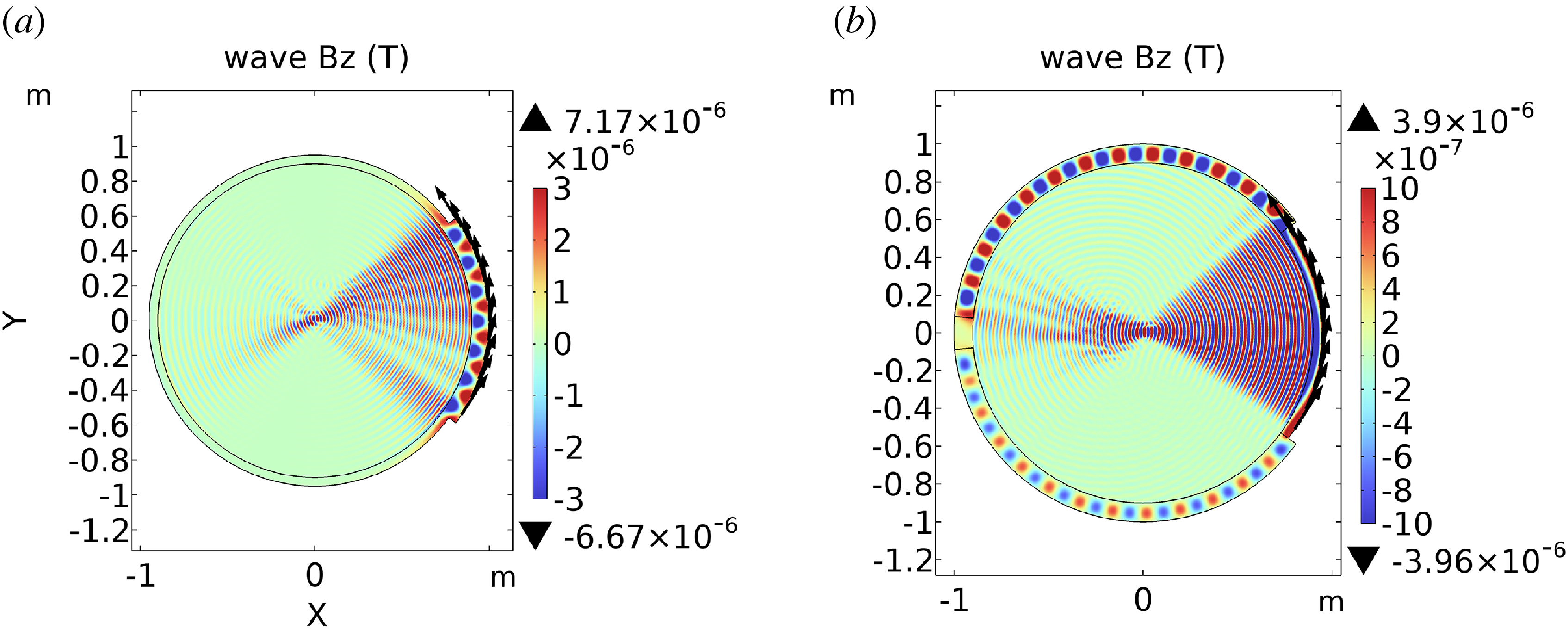
Figure 13. Long description
Two contour plots illustrate the wave Bz in Tesla, showing the impact of reducing the Scrape-Off Layer width on wave propagation. Panel A: The contour plot shows wave Bz with the Scrape-Off Layer width reduced outside the antenna extent. The x-axis ranges from -1 to 1 meters, and the y-axis ranges from -1.2 to 1.2 meters. The color scale ranges from -6.67e-6 to 7.17e-6 Tesla. Panel B: The contour plot shows wave Bz with the Scrape-Off Layer width reduced within the antenna extent. The x-axis ranges from -1 to 1 meters, and the y-axis ranges from -1.2 to 1.2 meters. The color scale ranges from -3.96e-6 to 3.9e-6 Tesla. Both plots indicate changes in wave propagation patterns due to the reduction in Scrape-Off Layer width.
3. Effect of spatially varying axial magnetic field on SOL waveguide modes
In this section, the effect of the 2-D magnetic-field geometry on the SOL waveguide mode is examined by introducing a tokamak-like spatially varying axial B-field, whose magnitude decreases with increasing x-coordinate in the model. The question is whether the geometric cutoff condition continues to control the SOL waveguide mode when the wave perpendicular wavelength varies ‘major radially’. For this purpose, the background axial B-field is modified as follows:
 \begin{equation} B_{z} (x)= \frac {1}{x+1.5}, \end{equation}
so that the B-field is inversely proportional to the ‘major radial’ coordinate, as shown in figure 15(a). The magnetic field remains at 0.4 T at the outboard midplane, where the antenna centre is located. The field increases up to 2 T at the ‘inboard’ side of the model (x = –1 m). The field direction remains axial only. For the input $k_z$
= 3
$k_z$
= 3 $\mathrm{m}^{-1}$
, the half-wavelength condition is no longer supported inside x
$\mathrm{m}^{-1}$
, the half-wavelength condition is no longer supported inside x $\approx$
0.26 m.
$\approx$
0.26 m.
Control of the propagating SOL waveguide mode by an increase of the background B-field from 0.4 to 0.8 T. Here, $k_z$
= 3
$k_z$
= 3 $\mathrm{m}^{-1}$
.Other parameters are identical to those in figure 1.
$\mathrm{m}^{-1}$
.Other parameters are identical to those in figure 1.
(a) Axial B-field profile as introduced in § 3. The vertical dashed line indicates that the geometric SOL half-wavelength condition for $k_z$
= 3
$k_z$
= 3 $\mathrm{m}^{-1}$
is satisfied at B
$\mathrm{m}^{-1}$
is satisfied at B $\lt$
0.56 T (x
$\lt$
0.56 T (x $\gt$
0.26 m) only. (b) Corresponding wave
$\gt$
0.26 m) only. (b) Corresponding wave $B_z$
profile. The SOL transport mode is observed only up to x
$B_z$
profile. The SOL transport mode is observed only up to x $\approx$
0.26 m.
$\approx$
0.26 m.
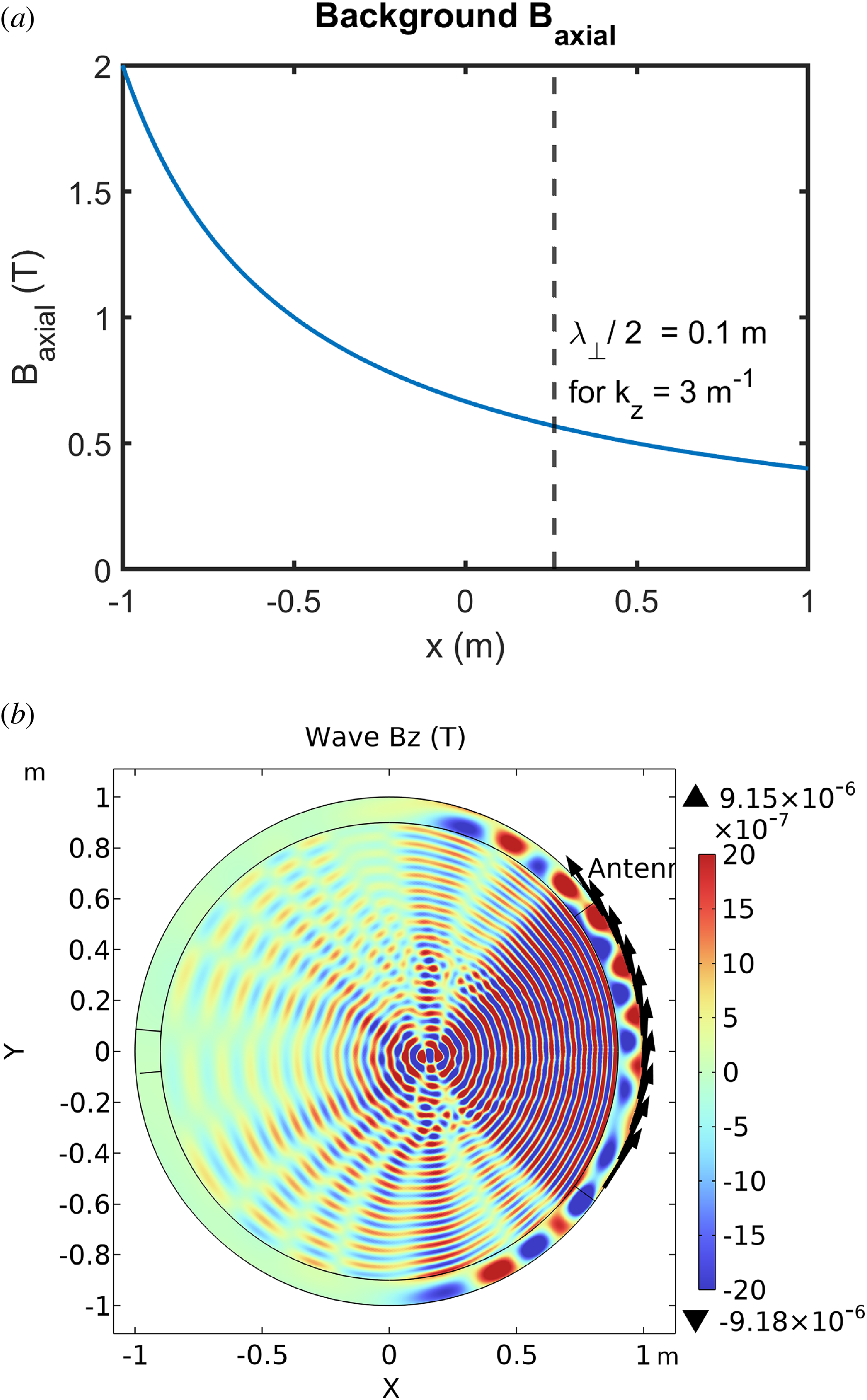
Figure 15(b) shows the wave axial magnetic field at $k_z$
= 3
$k_z$
= 3 $\mathrm{m}^{-1}$
. In contrast to the uniform B-field case in figure 1, the SOL propagation is restricted to x
$\mathrm{m}^{-1}$
. In contrast to the uniform B-field case in figure 1, the SOL propagation is restricted to x $\gtrsim$
0.26 m (
$\gtrsim$
0.26 m ( $B_{z} \lesssim$
0.56 T) well before reaching the conductive loss region at
$B_{z} \lesssim$
0.56 T) well before reaching the conductive loss region at $175^{\circ } \leqslant \theta \leqslant 185^{\circ }$
. For higher magnetic-field strengths, the azimuthal wavelength of the SOL mode increases and eventually becomes evanescent. As shown in figure 16, the peak azimuthal mode number of the tangential wave electric field outside the antenna is reduced to m
$175^{\circ } \leqslant \theta \leqslant 185^{\circ }$
. For higher magnetic-field strengths, the azimuthal wavelength of the SOL mode increases and eventually becomes evanescent. As shown in figure 16, the peak azimuthal mode number of the tangential wave electric field outside the antenna is reduced to m $ \approx \pm 20$
, and becomes broader as the local B-field strength is continuously increased away from the antenna. The azimuthal spectrum for the wavefield inside the antenna extent(
$ \approx \pm 20$
, and becomes broader as the local B-field strength is continuously increased away from the antenna. The azimuthal spectrum for the wavefield inside the antenna extent( $|\theta |\lt 36^{\circ }$
) still exhibits resonant peaks at a high
$|\theta |\lt 36^{\circ }$
) still exhibits resonant peaks at a high $|m|$
(m
$|m|$
(m $\approx$
34 and –28), in line with the resonant mode numbers found in the uniform B-field case.
$\approx$
34 and –28), in line with the resonant mode numbers found in the uniform B-field case.
Azimuthal spectrum of the wave $E_\theta$
along the circumference at r = 0.95 m in the middle of the annular SOL for
$E_\theta$
along the circumference at r = 0.95 m in the middle of the annular SOL for $k_z$
= 3
$k_z$
= 3 $\mathrm{m}^{-1}$
in the presence of the spatially varying background magnetic field as shown in figure 15 (a). Here,
$\mathrm{m}^{-1}$
in the presence of the spatially varying background magnetic field as shown in figure 15 (a). Here, $k_z$
= 3
$k_z$
= 3 $\mathrm{m}^{-1}$
.
$\mathrm{m}^{-1}$
.

More importantly, the mode-number analysis reveals that, at these resonant m values, the SOL power transported along the azimuthal direction becomes eventually redirected radially into the core plasma at the azimuthal position where the half-wavelength condition is no longer satisfied. This is illustrated in the spatial profile of the wave tangential electric field at $m_0=$
–28 and +34, as shown in figure 17. In the
$m_0=$
–28 and +34, as shown in figure 17. In the $m_0$
= –28 case, the clockwise azimuthal propagation, initiated at the antenna, is clearly observed in the annular SOL, and becomes evanescent near x = 0.26 m near the plasma bottom. At this location, a lobe of the wave tangential electric field appears and propagates radially inward. Similarly, in the
$m_0$
= –28 case, the clockwise azimuthal propagation, initiated at the antenna, is clearly observed in the annular SOL, and becomes evanescent near x = 0.26 m near the plasma bottom. At this location, a lobe of the wave tangential electric field appears and propagates radially inward. Similarly, in the $m_0$
= +34 case, the counterclockwise azimuthal propagation up to the evanescent location near the plasma top is redirected into the core plasma. This behaviour is understood as power redirection since annular SOL no longer supports the bounded mode in the higher B-field region.
$m_0$
= +34 case, the counterclockwise azimuthal propagation up to the evanescent location near the plasma top is redirected into the core plasma. This behaviour is understood as power redirection since annular SOL no longer supports the bounded mode in the higher B-field region.
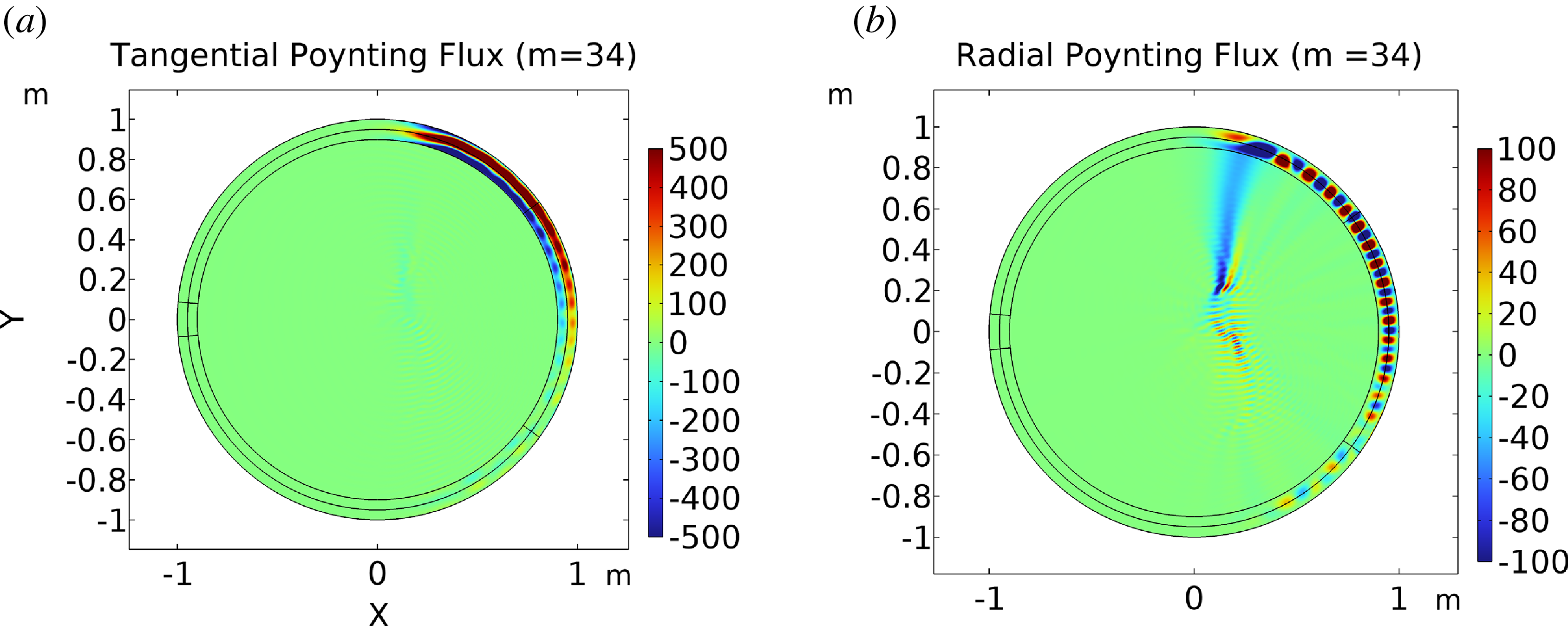
This interpretation is supported by the spatial distributions of the tangential and radial Poynting fluxes for $m_0$
= +34. As shown in figure 18(a), the azimuthal component of Poynting flux is localised within the annular SOL and exhibits an asymmetrical distribution only in the upper half of the plasma, which then decays near the evanescent position. At this location, the radially inward component of Poynting flux appears, as shown in figure 18(b). This feature is absent in the uniform B-field case, where the SOL waveguide mode is supported continuously around the circumference.
$m_0$
= +34. As shown in figure 18(a), the azimuthal component of Poynting flux is localised within the annular SOL and exhibits an asymmetrical distribution only in the upper half of the plasma, which then decays near the evanescent position. At this location, the radially inward component of Poynting flux appears, as shown in figure 18(b). This feature is absent in the uniform B-field case, where the SOL waveguide mode is supported continuously around the circumference.
Response of the wave tangential electric field ( $E_\theta$
) to the to the antenna current source:
$E_\theta$
) to the to the antenna current source: $\boldsymbol{j}_\theta =\hat {\theta } \mathrm{exp}(im_0\theta )$
for (a)
$\boldsymbol{j}_\theta =\hat {\theta } \mathrm{exp}(im_0\theta )$
for (a) $m_0$
= –28 and (b)
$m_0$
= –28 and (b) $m_0$
= +34, in the presence of the spatially varying background magnetic field. Here,
$m_0$
= +34, in the presence of the spatially varying background magnetic field. Here, $k_z$
= 3
$k_z$
= 3 $\mathrm{m}^{-1}$
. The antenna azimuthal extent is indicated by a set of antenna current vectors.
$\mathrm{m}^{-1}$
. The antenna azimuthal extent is indicated by a set of antenna current vectors.
(a) Tangential and (b) radial components of Poynting flux for the $m_0$
= +34 case in figure 17(b).
$m_0$
= +34 case in figure 17(b).
Contribution of these high-m components to the wavefield is clearly observed in the total wave magnetic field in figure 15(b). In the $x \gt 0$
region, multiple secondary lobes are observed outside the antenna azimuthal extent, starting from the core/SOL interface layer. These features are in addition to the main lobe that spans the antenna extent (
$x \gt 0$
region, multiple secondary lobes are observed outside the antenna azimuthal extent, starting from the core/SOL interface layer. These features are in addition to the main lobe that spans the antenna extent ( $|\theta | \lt 36^ {\circ }$
). The strength of these high-m contributions is weighted by the antenna spectrum and the degree of resonant SOL coupling. These additional lobes are at a much lower level and nearly absent in the uniform B-field case, as shown in figure 1, indicating that SOL transport can modify not only the spectral content but also the spatial distribution of the wave field.
$|\theta | \lt 36^ {\circ }$
). The strength of these high-m contributions is weighted by the antenna spectrum and the degree of resonant SOL coupling. These additional lobes are at a much lower level and nearly absent in the uniform B-field case, as shown in figure 1, indicating that SOL transport can modify not only the spectral content but also the spatial distribution of the wave field.
4. Effect of poloidal magnetic field on SOL waveguide modes
In this section, an azimuthal B-field is further superimposed on the spatially varying axial B-field to further examine the impact of the ‘poloidal’ field on the SOL waveguide mode. The presence of the poloidal field breaks the symmetry between the positive and negative poloidal mode numbers, which can modify the local $k_\parallel$
and the plasma dispersion. For this purpose, the following radially varying circular poloidal field is added
$k_\parallel$
and the plasma dispersion. For this purpose, the following radially varying circular poloidal field is added
 \begin{equation} \boldsymbol{B_p} = 0.1\times r (-\mathrm{sin}\theta \,\hat {x} +\mathrm{cos}\theta \,\hat {y}), \end{equation}
where $0\leqslant r \leqslant 1\, (\mathrm{m})$
such that it is minimum (
$0\leqslant r \leqslant 1\, (\mathrm{m})$
such that it is minimum ( $B_p$
= 0) at r = 0 m and maximum (
$B_p$
= 0) at r = 0 m and maximum ( $B_p$
= 0.1 T) at r = 1 m. The axial B-field profiles remain the same as in § 3. Adding the azimuthal field increases the local B-field by at most 12
$B_p$
= 0.1 T) at r = 1 m. The axial B-field profiles remain the same as in § 3. Adding the azimuthal field increases the local B-field by at most 12 $\%$
at x = 1 m. The magnetic geometry is now closer to a more tokamak-like configuration in the limit of a large aspect ratio.
$\%$
at x = 1 m. The magnetic geometry is now closer to a more tokamak-like configuration in the limit of a large aspect ratio.
Figure 19 presents the wave magnetic field for $k_z = 3\, \mathrm{m}^{-1}$
, which can be compared with the uniform axial magnetic-field case in figure 1 and with the
$k_z = 3\, \mathrm{m}^{-1}$
, which can be compared with the uniform axial magnetic-field case in figure 1 and with the $1/x$
-dependent axial field only case in figure 15. In the core plasma, the up–down-asymmetric helical trajectory of the wave phase front indicates the presence of a relatively weak but finite poloidal field. In the annular SOL, the poloidal extent of the SOL mode is observed up to x
$1/x$
-dependent axial field only case in figure 15. In the core plasma, the up–down-asymmetric helical trajectory of the wave phase front indicates the presence of a relatively weak but finite poloidal field. In the annular SOL, the poloidal extent of the SOL mode is observed up to x $\approx$
0.3 m, in line with the results from the previous section on the role of the increasing B-field at a smaller x. Additional lobes outside the antenna extent are observed as well.
$\approx$
0.3 m, in line with the results from the previous section on the role of the increasing B-field at a smaller x. Additional lobes outside the antenna extent are observed as well.
Wave $B_z$
profile in the presence of the background poloidal and 1/x-dependent axial B-field. Here,
$B_z$
profile in the presence of the background poloidal and 1/x-dependent axial B-field. Here, $k_z$
= 3
$k_z$
= 3 $\mathrm{m}^{-1}$
.
$\mathrm{m}^{-1}$
.

Area-integrated axial Poynting flux in both the core and annular SOL regions as a function of $m_0$
of the poloidal phase factor
$m_0$
of the poloidal phase factor $\exp (im_0\theta )$
that is multiplied to the antenna current function. Here,
$\exp (im_0\theta )$
that is multiplied to the antenna current function. Here, $k_z$
= 3
$k_z$
= 3 $\mathrm{m}^{-1}$
. Analytic estimates,
$\mathrm{m}^{-1}$
. Analytic estimates, $m_{est}$
, from the generalised dispersion condition are indicated by the vertical dashed lines.
$m_{est}$
, from the generalised dispersion condition are indicated by the vertical dashed lines.

A more pronounced effect of the poloidal B-field is the reduction of the azimuthal mode number observed in the annular SOL. To identify the resonant poloidal mode numbers in the annular SOL, the numerical mode analysis is conducted. The resulting area-integrated axial Poynting flux is shown as a function of $m_0$
in figure 20. In addition to the peak at
$m_0$
in figure 20. In addition to the peak at $m_0\approx -2$
, which predominantly produces low-m components and primarily determines the wavefield right in front of the antenna, there are two additional resonant values at
$m_0\approx -2$
, which predominantly produces low-m components and primarily determines the wavefield right in front of the antenna, there are two additional resonant values at $m_0 \approx -26$
and
$m_0 \approx -26$
and $m_0 \approx +17$
. These m-numbers are lower and more asymmetric than those found in the previous two sections, despite a small addition of the poloidal field. The field-line tilt can alter the local dispersion and, therefore, the local conditions of the half-wavelength fit in the annular SOL. These resonant
$m_0 \approx +17$
. These m-numbers are lower and more asymmetric than those found in the previous two sections, despite a small addition of the poloidal field. The field-line tilt can alter the local dispersion and, therefore, the local conditions of the half-wavelength fit in the annular SOL. These resonant $m_0$
values reasonably agree well with those from the fast-wave dispersion that is explicitly written for a non-field-aligned geometry (Bertelli et al. Reference Bertelli2014)
$m_0$
values reasonably agree well with those from the fast-wave dispersion that is explicitly written for a non-field-aligned geometry (Bertelli et al. Reference Bertelli2014)
 \begin{align} {\big[N^2-{(\hat {e}_2 \boldsymbol{\cdot }\boldsymbol{N})}^2-S\big]} {\big[N^2-{(\hat {e}_3 \boldsymbol{\cdot }\boldsymbol{N})}^2-S\big]} - {\big[D^2+{(\hat {e}_2 \boldsymbol{\cdot }\boldsymbol{N})}^2{(\hat {e}_3\boldsymbol{\cdot }\boldsymbol{N})}^2\big]} = 0, \end{align}
where the three basis vectors are deliberately chosen: $\hat {e}_1 = \hat {b}$
,
$\hat {e}_1 = \hat {b}$
, $\hat {e}_2 = \hat {r} \times \hat {b} /|\hat {r} \times \hat {b}|$
and
$\hat {e}_2 = \hat {r} \times \hat {b} /|\hat {r} \times \hat {b}|$
and $\hat {e}_3 = \hat {e}_1 \times \hat {e}_2$
. The total refractive index,
$\hat {e}_3 = \hat {e}_1 \times \hat {e}_2$
. The total refractive index, $\boldsymbol{N}=(c/\omega )\boldsymbol{k}$
is expressed in the reference spatial coordinate system:
$\boldsymbol{N}=(c/\omega )\boldsymbol{k}$
is expressed in the reference spatial coordinate system: $\boldsymbol{N}=N_r \hat {r}+N_\theta \hat {\theta }+ N_z \hat {z}$
. This dispersion relation is reduced to the quadratic form in (2.2) in the axial B-field only case. In the presence of the poloidal field, the dispersion relation can be written as a fourth-order polynomial equation for the unknown
$\boldsymbol{N}=N_r \hat {r}+N_\theta \hat {\theta }+ N_z \hat {z}$
. This dispersion relation is reduced to the quadratic form in (2.2) in the axial B-field only case. In the presence of the poloidal field, the dispersion relation can be written as a fourth-order polynomial equation for the unknown $k_\theta$
under the assumption that the radial half-wavelength eigenmode structure is imposed
$k_\theta$
under the assumption that the radial half-wavelength eigenmode structure is imposed $k_r = \pi /\varDelta$
. The corresponding roots (the real part only) are shown in figure 21 as a function of the applied
$k_r = \pi /\varDelta$
. The corresponding roots (the real part only) are shown in figure 21 as a function of the applied $B_\theta$
for a fixed
$B_\theta$
for a fixed $B_z$
= 0.4 T. At
$B_z$
= 0.4 T. At $B_\theta$
= 0, the poloidal modes at m
$B_\theta$
= 0, the poloidal modes at m $=\pm 33$
are supported as seen in § 2. Interestingly, the poloidal mode numbers converge to a low-m range as the pitch angle increases toward
$=\pm 33$
are supported as seen in § 2. Interestingly, the poloidal mode numbers converge to a low-m range as the pitch angle increases toward $45^{\circ }$
(
$45^{\circ }$
( $B_{\theta }$
= 0.4 T), implying that a higher level of SOL mode excitation may occur due to the increased power in the lower-m components of the antenna spectrum (figure 2).
$B_{\theta }$
= 0.4 T), implying that a higher level of SOL mode excitation may occur due to the increased power in the lower-m components of the antenna spectrum (figure 2).
Analytic m-roots found as a function of $B_\theta$
for
$B_\theta$
for $k_z = 3\,\mathrm{m}^{-1}$
. Here,
$k_z = 3\,\mathrm{m}^{-1}$
. Here, $B_z$
= 0.4 T,
$B_z$
= 0.4 T, $n_e=3\times 10^{18}\,\mathrm{m}^{-3}$
,
$n_e=3\times 10^{18}\,\mathrm{m}^{-3}$
, $r_{\textit{eff}}$
= 0.95 m and
$r_{\textit{eff}}$
= 0.95 m and $k_r = \pi /\varDelta$
, where
$k_r = \pi /\varDelta$
, where $\varDelta = 0.1\,\mathrm{m}$
. The real part of the roots are shown.
$\varDelta = 0.1\,\mathrm{m}$
. The real part of the roots are shown.
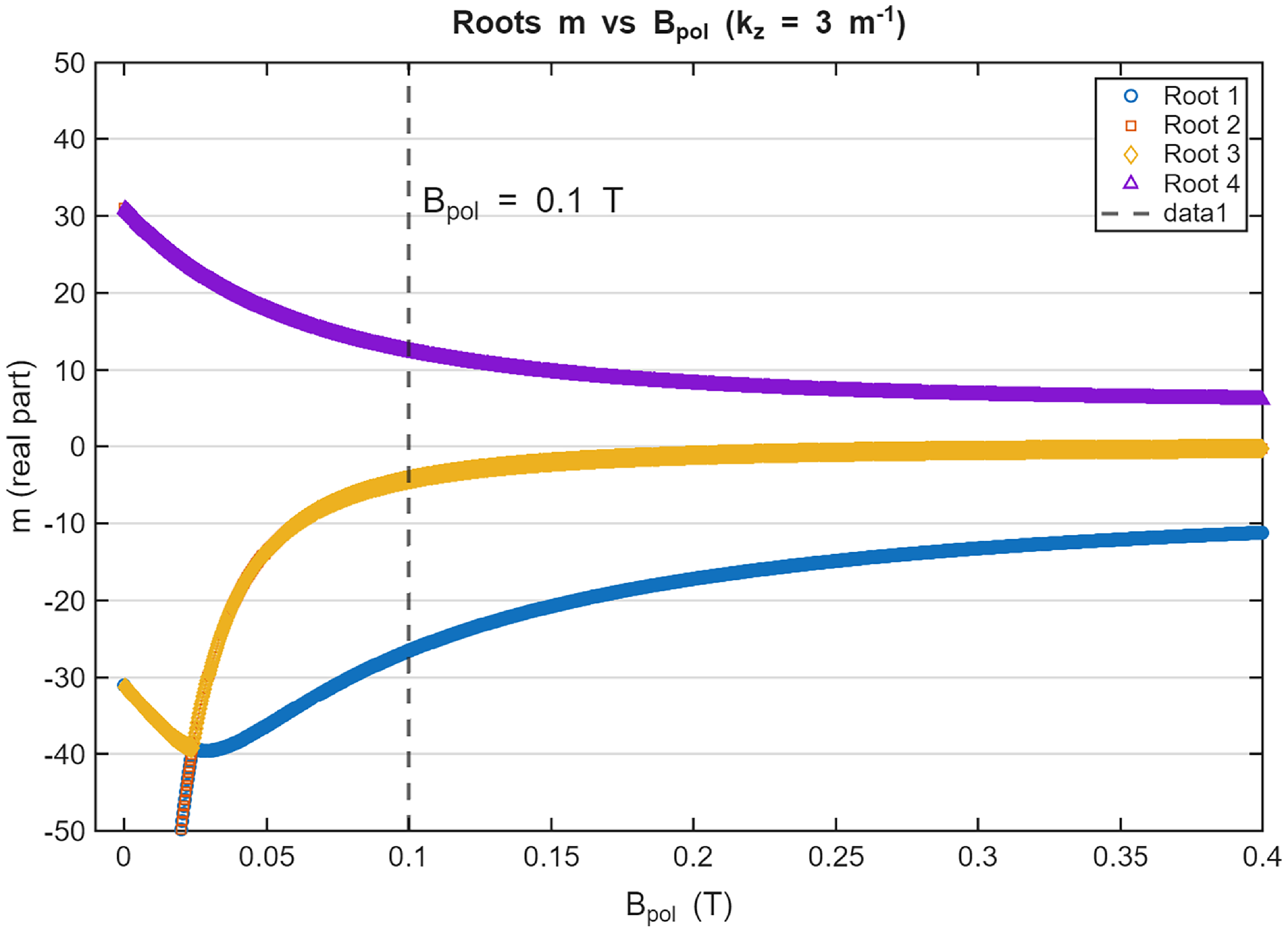
The three roots found at $B_\theta$
= 0.1 T are shown as vertical dashed lines in figure 20, and agree well with the 2-D numerical results. The m = –4 root is a complex-conjugate pair, which is excited but strongly evanescent near the antenna. The remaining roots (m = 14 and –27) are real valued. This consistency indicates that the SOL plasma selects poloidal eigenmodes supported by the local dispersion. The local eigenmode condition is now modified since the parallel wavenumber is modified by the coupling of the high-m mode to the local poloidal B-field. The
$B_\theta$
= 0.1 T are shown as vertical dashed lines in figure 20, and agree well with the 2-D numerical results. The m = –4 root is a complex-conjugate pair, which is excited but strongly evanescent near the antenna. The remaining roots (m = 14 and –27) are real valued. This consistency indicates that the SOL plasma selects poloidal eigenmodes supported by the local dispersion. The local eigenmode condition is now modified since the parallel wavenumber is modified by the coupling of the high-m mode to the local poloidal B-field. The $k_{\parallel }$
is now the projection of two components of
$k_{\parallel }$
is now the projection of two components of $k_z$
and
$k_z$
and $k_\theta$
 \begin{equation} k_{\parallel } = \frac {k_z B_z + (m/r)B_\theta }{|B|} ,\end{equation}
where $k_\theta = m/r$
. The impact of the modified
$k_\theta = m/r$
. The impact of the modified $k_\parallel$
is also seen by the reversed direction of the axial Poynting flux in the annular SOL at
$k_\parallel$
is also seen by the reversed direction of the axial Poynting flux in the annular SOL at $m_0 \approx -26$
. A negative poloidal mode number can generate a negative
$m_0 \approx -26$
. A negative poloidal mode number can generate a negative $k_\parallel$
. In this case,
$k_\parallel$
. In this case, $k_\parallel$
becomes –3.4 and +7.0 for the given
$k_\parallel$
becomes –3.4 and +7.0 for the given $m_0 = -26$
and +17, respectively. The spectral content of
$m_0 = -26$
and +17, respectively. The spectral content of $k_\parallel$
is mixed in the annular SOL. Interestingly, at
$k_\parallel$
is mixed in the annular SOL. Interestingly, at $m = -26$
, the integrated axial-flow power direction in the SOL is reversed.
$m = -26$
, the integrated axial-flow power direction in the SOL is reversed.
Response of the wave poloidal (tangential) electric field ( $E_\theta$
) to the antenna current source:
$E_\theta$
) to the antenna current source: $\boldsymbol{j}_\theta =\hat {\theta }\,\mathrm{exp}(im_0\theta )$
, where
$\boldsymbol{j}_\theta =\hat {\theta }\,\mathrm{exp}(im_0\theta )$
, where $\hat {\theta }=-\mathrm{sin}\theta \,\hat {x}+\mathrm{cos}\theta \,\hat {y}$
, for (a)
$\hat {\theta }=-\mathrm{sin}\theta \,\hat {x}+\mathrm{cos}\theta \,\hat {y}$
, for (a) $m_0$
= –26 and (b)
$m_0$
= –26 and (b) $m_0$
= +17, in the presence of both the axial and poloidal B-field. Here,
$m_0$
= +17, in the presence of both the axial and poloidal B-field. Here, $k_z$
= 3
$k_z$
= 3 $\mathrm{m}^{-1}$
. The antenna poloidal extent is indicated by a set of antenna current vectors.
$\mathrm{m}^{-1}$
. The antenna poloidal extent is indicated by a set of antenna current vectors.

Figure 22 shows the poloidal wave electric fields excited with the imposed poloidal phase factor $\exp (im_0\theta )$
of
$\exp (im_0\theta )$
of $m_0$
= –26 and +17 to the antenna current source. The field is resonantly coupled to the SOL. The field pattern can be understood in a similar way to the previous sections. First, the azimuthal extent of the propagating SOL mode is limited by the local magnetic-field magnitude (mostly toroidal component here). With the imposed phase factor at
$m_0$
= –26 and +17 to the antenna current source. The field is resonantly coupled to the SOL. The field pattern can be understood in a similar way to the previous sections. First, the azimuthal extent of the propagating SOL mode is limited by the local magnetic-field magnitude (mostly toroidal component here). With the imposed phase factor at $m_0$
= –26, the evanescent position of the annulus SOL mode is near the bottom of the plasma, which coincides with the location where the power is redirected into the propagating fast wave in the core. Similarly, for
$m_0$
= –26, the evanescent position of the annulus SOL mode is near the bottom of the plasma, which coincides with the location where the power is redirected into the propagating fast wave in the core. Similarly, for $m_0 = 17$
, the mode becomes evanescent just above the top end of the antenna section, while it has a longer poloidal wavelength due to a lower poloidal mode number. In both cases, there is a lobe of core wavefield, generated at that evanescent location. The influence of high-m components on the final wavefield is seen in figure 19, particularly in the top region of the antenna extent. It can also be seen that the low-m poloidal structure modulates the spatial pattern of the core wavefield.
$m_0 = 17$
, the mode becomes evanescent just above the top end of the antenna section, while it has a longer poloidal wavelength due to a lower poloidal mode number. In both cases, there is a lobe of core wavefield, generated at that evanescent location. The influence of high-m components on the final wavefield is seen in figure 19, particularly in the top region of the antenna extent. It can also be seen that the low-m poloidal structure modulates the spatial pattern of the core wavefield.
Azimuthal Fourier transform of the tangential electric fields along the radius at r = 0.95 m in the middle of the annular SOL for the two cases applied at $m_0$
= –26 and +17, shown in figure 22. The azimuthal spectrum at
$m_0$
= –26 and +17, shown in figure 22. The azimuthal spectrum at $m_0$
= 0 is also shown. For an antenna azimuthal phase factor of
$m_0$
= 0 is also shown. For an antenna azimuthal phase factor of $m_0 = 17$
, the antenna spectrum continues to seed the
$m_0 = 17$
, the antenna spectrum continues to seed the $m \approx -26$
component, and the annular SOL supports and sustains that mode.
$m \approx -26$
component, and the annular SOL supports and sustains that mode.
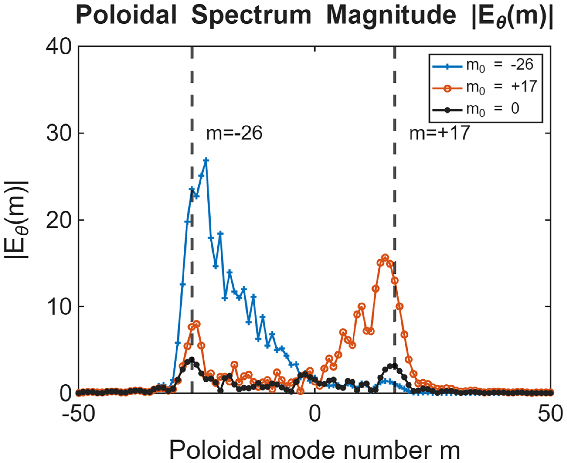
Because the local magnetic field is no longer aligned with the geometry due to the introduction of the poloidal magnetic field, the peak azimuthal phase factor applied by the antenna, $\exp (i m_0 \theta )$
, does not necessarily drive the SOL mode at that azimuthal phase (
$\exp (i m_0 \theta )$
, does not necessarily drive the SOL mode at that azimuthal phase ( $m\neq m_0$
). The finite extent of the antenna excites a range of poloidal harmonics, and the azimuthal phase of the SOL eigenmode is determined by the plasma dispersion and magnetic geometries. Figure 23 shows the azimuthal Fourier transform of the tangential electric fields along the radius at r = 0.95 m in the middle of the annular SOL for the two cases at
$m\neq m_0$
). The finite extent of the antenna excites a range of poloidal harmonics, and the azimuthal phase of the SOL eigenmode is determined by the plasma dispersion and magnetic geometries. Figure 23 shows the azimuthal Fourier transform of the tangential electric fields along the radius at r = 0.95 m in the middle of the annular SOL for the two cases at $m_0$
= –26 and + 17. For
$m_0$
= –26 and + 17. For $m_0 =$
–26, the peak azimuthal mode supported by the annular SOL is nearly matched to the imposed antenna azimuthal phase. However, for
$m_0 =$
–26, the peak azimuthal mode supported by the annular SOL is nearly matched to the imposed antenna azimuthal phase. However, for $m_0$
= 17, there is a secondary mode supported at m
$m_0$
= 17, there is a secondary mode supported at m $\approx$
–26, in addition to the primary peak at m
$\approx$
–26, in addition to the primary peak at m $\approx$
17. The antenna spectrum excites this component, which is selected and amplified by the annular SOL.
$\approx$
17. The antenna spectrum excites this component, which is selected and amplified by the annular SOL.
(a) Wave $B_z$
and (b)
$B_z$
and (b) $E_\theta$
for
$E_\theta$
for $k_z$
= 7
$k_z$
= 7 $\mathrm{m}^{-1}$
in the presence of the background poloidal and 1/x-dependent axial B-field.
$\mathrm{m}^{-1}$
in the presence of the background poloidal and 1/x-dependent axial B-field.
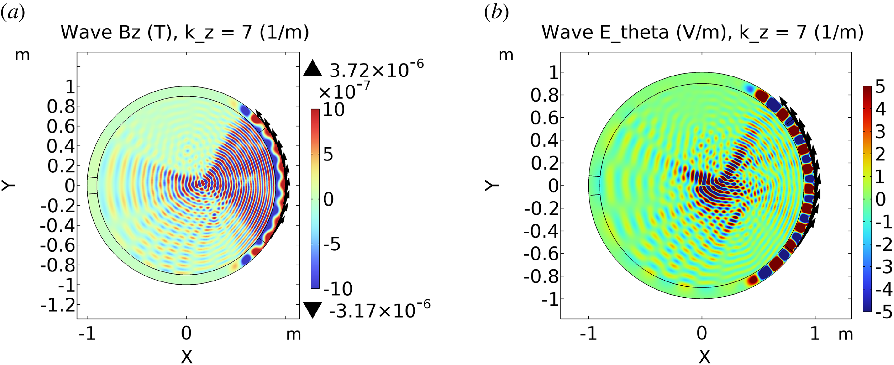
Azimuthal Fourier transform of the tangential electric field along the radius at r = 0.95 m, taken at the midplane of the annular SOL, for $k_z$
= 7
$k_z$
= 7 $\mathrm{m^{-1}}$
at the antenna azimuthal phase factor
$\mathrm{m^{-1}}$
at the antenna azimuthal phase factor $m_0$
= 0, as shown in figure 24(b). Three analytic m-estimates from the generalised dispersion are indicated by the vertical dashed lines.
$m_0$
= 0, as shown in figure 24(b). Three analytic m-estimates from the generalised dispersion are indicated by the vertical dashed lines.
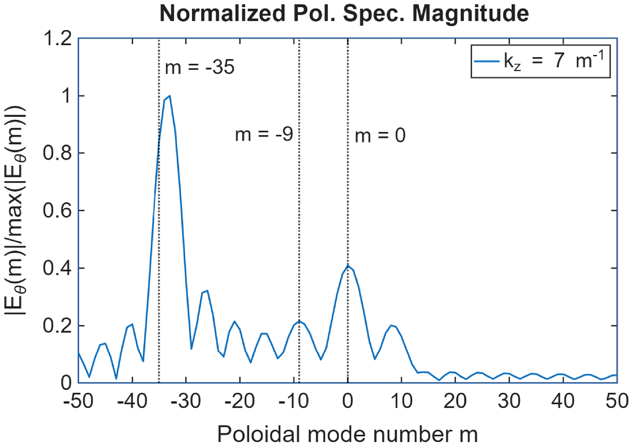
For completeness, the $k_z$
= 7
$k_z$
= 7 $\mathrm{m}^{-1}$
case is briefly discussed, which provides another example of the plasma mode selection when the SOL eigenmode is driven by the antenna boundary. As shown by the wave
$\mathrm{m}^{-1}$
case is briefly discussed, which provides another example of the plasma mode selection when the SOL eigenmode is driven by the antenna boundary. As shown by the wave $B_z$
and
$B_z$
and $E_\theta$
in figure 24, a higher |m|-number structure is observed, which is absent in the uniform background B-field case. The corresponding poloidal spectrum shown in figure 25 shows that the poloidal mode at
$E_\theta$
in figure 24, a higher |m|-number structure is observed, which is absent in the uniform background B-field case. The corresponding poloidal spectrum shown in figure 25 shows that the poloidal mode at $m\approx -33$
is dominantly excited in the annular SOL. The analytic roots from (4.2) found at m
$m\approx -33$
is dominantly excited in the annular SOL. The analytic roots from (4.2) found at m $\approx$
–35, –9 and 0 are consistent with the numerical modelling. The root at m = –9 is a complex conjugate pair, whereas the roots at m = –35 and 0 are real valued, responsible for the mode structure supported within the annular SOL.
$\approx$
–35, –9 and 0 are consistent with the numerical modelling. The root at m = –9 is a complex conjugate pair, whereas the roots at m = –35 and 0 are real valued, responsible for the mode structure supported within the annular SOL.
5. Two-dimensional axisymmetric HHFW modelling using NSTX-U geometry
This section extends the previous sections by adopting a 2-D axisymmetric geometry for the NSTX-U plasma configuration to demonstrate that the eigenmode features identified in the simplified circular model remain in an experimentally relevant NSTX-U configuration. The axisymmetric system imposes that the toroidal wavenumber scales as $k_\phi = N_\phi /R$
, and this local increase in
$k_\phi = N_\phi /R$
, and this local increase in $k_\phi$
at a smaller R can suppress bounded-mode propagation even when the transverse dimensions of the two SOL boundaries remain fixed. This section examines the mode-propagation behaviour between the plasma-shape-confirming wall boundary and the real wall boundary with a varying width. Finally, by adopting a realistic H-mode density profile, it is shown that the SOL eigenmode is suppressed at NSTX-U field strength (
$k_\phi$
at a smaller R can suppress bounded-mode propagation even when the transverse dimensions of the two SOL boundaries remain fixed. This section examines the mode-propagation behaviour between the plasma-shape-confirming wall boundary and the real wall boundary with a varying width. Finally, by adopting a realistic H-mode density profile, it is shown that the SOL eigenmode is suppressed at NSTX-U field strength ( $B_0 = 1$
T) compared with that of NSTX (
$B_0 = 1$
T) compared with that of NSTX ( $B_0$
= 0.5 T).
$B_0$
= 0.5 T).
The HHFW wavefield with a plasma-shaped conforming wall boundary at three different background magnetic fields: (a) toroidal B-field only at 0.4 T, (b) 1/R toroidal-B variation and (c) 1/R toroidal-B variation and poloidal field ( $B_{\theta ,max}$
= 0.1 T). The outer black curve is a PEC wall, and the inner blue curve is the LCFS. The antenna region at the outboard midplane is shown in cyan. Here,
$B_{\theta ,max}$
= 0.1 T). The outer black curve is a PEC wall, and the inner blue curve is the LCFS. The antenna region at the outboard midplane is shown in cyan. Here, $N_\phi$
= 5, corresponding to
$N_\phi$
= 5, corresponding to $k_\phi = N_\phi /R_{ant} \approx 3.24\, \mathrm{m^{-1}}$
with
$k_\phi = N_\phi /R_{ant} \approx 3.24\, \mathrm{m^{-1}}$
with $R_{ant}$
= 1.54 m in the SOL.
$R_{ant}$
= 1.54 m in the SOL.
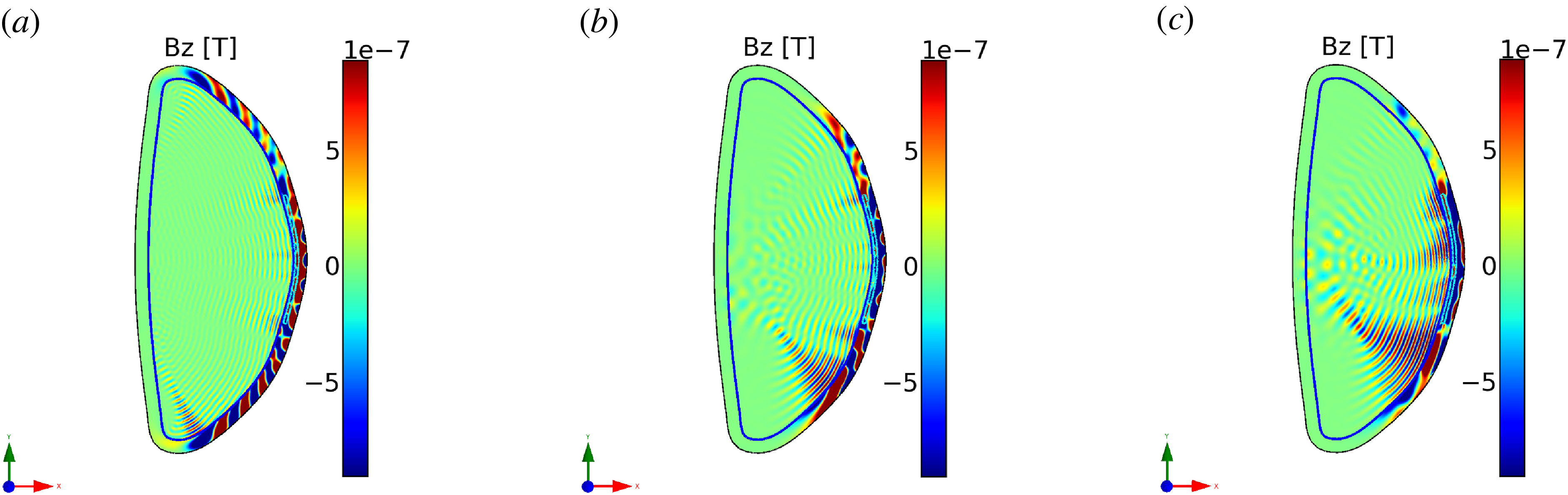
Figure 26 shows the HHFW magnetic wavefield ( $B_\phi$
) spatial profile when a plasma-shaped confirming wall boundary is imposed outside the LCFS at three different background magnetic fields: (a) toroidal B-field only at 0.4 T, (b) tokamak-like 1/R major-radial variation of the toroidal B-field while matching the toroidal B-field at the antenna at 0.4 T and (c) further superimposing the poloidal B-field that is maximum (0.1 T) at
$B_\phi$
) spatial profile when a plasma-shaped confirming wall boundary is imposed outside the LCFS at three different background magnetic fields: (a) toroidal B-field only at 0.4 T, (b) tokamak-like 1/R major-radial variation of the toroidal B-field while matching the toroidal B-field at the antenna at 0.4 T and (c) further superimposing the poloidal B-field that is maximum (0.1 T) at $\rho = 1$
. These parameters are to match those assumed in the cylinder models in the previous sections. The transverse gap width remains at 10 cm, and the core (SOL) density also remains constant at
$\rho = 1$
. These parameters are to match those assumed in the cylinder models in the previous sections. The transverse gap width remains at 10 cm, and the core (SOL) density also remains constant at $3\times 10^{19}\, (3\times 10^{18})\, \mathrm{m}^{-3}$
. The input
$3\times 10^{19}\, (3\times 10^{18})\, \mathrm{m}^{-3}$
. The input $N_\phi$
is 5, corresponding to
$N_\phi$
is 5, corresponding to $k_\phi = N_\phi /R_{ant} \approx 3.24\, \mathrm{m^{-1}}$
at the
$k_\phi = N_\phi /R_{ant} \approx 3.24\, \mathrm{m^{-1}}$
at the $R_{ant}$
= 1.54 m antenna location. In this geometry, the conductive loss region introduced in the SOL region at
$R_{ant}$
= 1.54 m antenna location. In this geometry, the conductive loss region introduced in the SOL region at $175^{\circ } \leqslant \theta \leqslant 185^{\circ }$
is no longer present. As shown in figure 26(a), even in the flat B-field case, the SOL mode becomes cutoff and evanescent at a smaller R where
$175^{\circ } \leqslant \theta \leqslant 185^{\circ }$
is no longer present. As shown in figure 26(a), even in the flat B-field case, the SOL mode becomes cutoff and evanescent at a smaller R where $k_\phi \approx 8\,\mathrm{m}^{-1}$
due to the local increase in
$k_\phi \approx 8\,\mathrm{m}^{-1}$
due to the local increase in $k_\phi$
in line with the features seen in the circular model. The power is redirected into the core near that region. When the major-radial variation of the toroidal magnetic field is introduced, the poloidal extent of the SOL waveguide mode is further reduced, as shown in figure 26 (b). Finally, figure 26(c) shows that, with the introduction of the poloidal field (the pitch), the mode structure becomes up–down asymmetric, consistent with the cylinder model analysis. The core spatial field pattern is strongly perturbed by the presence of the SOL mode.
$k_\phi$
in line with the features seen in the circular model. The power is redirected into the core near that region. When the major-radial variation of the toroidal magnetic field is introduced, the poloidal extent of the SOL waveguide mode is further reduced, as shown in figure 26 (b). Finally, figure 26(c) shows that, with the introduction of the poloidal field (the pitch), the mode structure becomes up–down asymmetric, consistent with the cylinder model analysis. The core spatial field pattern is strongly perturbed by the presence of the SOL mode.
The HHFW wavefield with a realistic wall boundary at three different background magnetic fields: (a) toroidal B only at 0.4 T, (b) 1/R toroidal-B variation and (c) 1/R toroidal-B variation and poloidal field ( $B_{\theta ,max}$
= 0.1 T). The outer black curve is a PEC wall, and the inner blue curve is the LCFS. The antenna region at the outboard midplane is shown in cyan. Here,
$B_{\theta ,max}$
= 0.1 T). The outer black curve is a PEC wall, and the inner blue curve is the LCFS. The antenna region at the outboard midplane is shown in cyan. Here, $N_\phi$
= 5, corresponding to
$N_\phi$
= 5, corresponding to $k_\phi = N_\phi /R_{ant} \approx 3.24\, \mathrm{m^{-1}}$
at the antenna
$k_\phi = N_\phi /R_{ant} \approx 3.24\, \mathrm{m^{-1}}$
at the antenna $R_{ant}$
= 1.54 m.
$R_{ant}$
= 1.54 m.
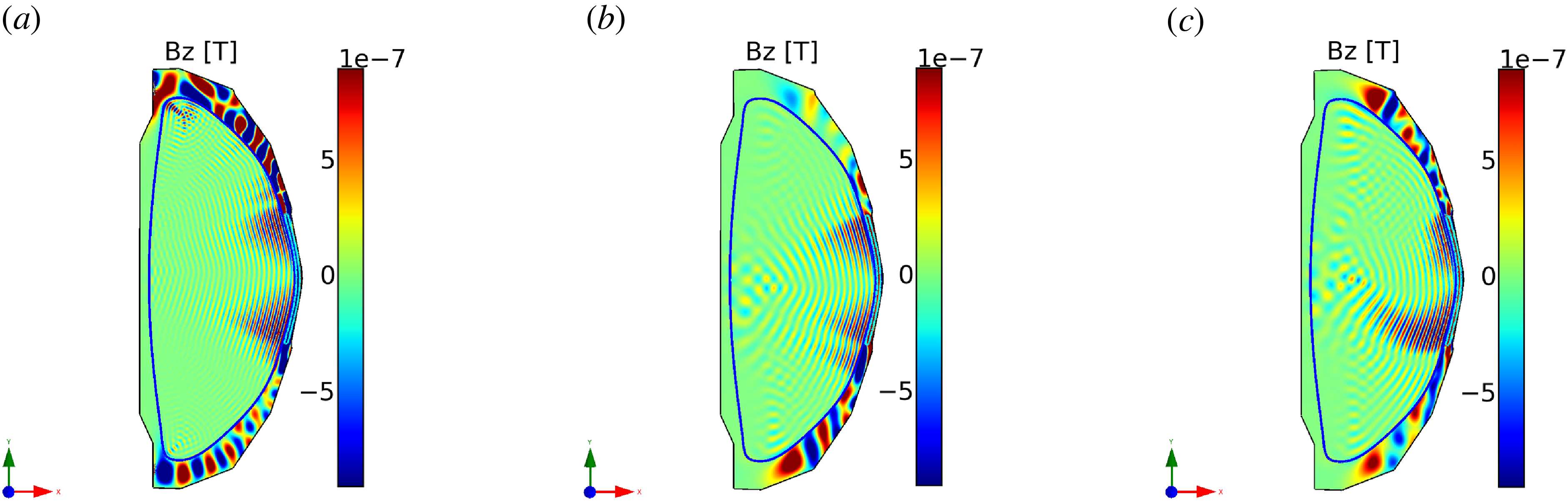
Figure 27 shows the HHFW magnetic wavefield ( $B_\phi$
) obtained instead using a realistic NSTX-U wall boundary for the same three background magnetic-field configurations. The realistic wall introduces a poloidally varying transverse gap between the LCFS and the conducting boundary, and its gap tends to increase away from the antenna, relaxing a half-wavelength condition. As shown in figure 27(a), even for the flat toroidal-field case, the SOL waveguide mode exhibits a larger poloidal extent, showing the local variation of the transverse geometric scale (the density remains the same in both cases). In this double-null magnetic configuration, X-points are also at the plasma top and bottom, which can complicate the mode structure due to a poloidal-field profile. When the major-radial variation of the toroidal magnetic field is introduced in figure 27(b), the SOL mode extent is reduced due to the local increase of the magnetic field. Finally, with the additional inclusion of the poloidal magnetic field in figure 27(c), the SOL mode is observed to deviate from a half-wavelength structure, while in this case, the poloidal extent remains more or less up–down symmetric. Although a constant SOL density is assumed here, these structures reproduce the trends and features of the SOL mode observed in a recent modelling study (De Levante Rodriguez et al. Reference De Levante Rodriguez, Baek, Shiraiwa, Bertelli and Bonoli2025), which employs a realistic divertor SOL density profile for NSTX/NSTX-U.
$B_\phi$
) obtained instead using a realistic NSTX-U wall boundary for the same three background magnetic-field configurations. The realistic wall introduces a poloidally varying transverse gap between the LCFS and the conducting boundary, and its gap tends to increase away from the antenna, relaxing a half-wavelength condition. As shown in figure 27(a), even for the flat toroidal-field case, the SOL waveguide mode exhibits a larger poloidal extent, showing the local variation of the transverse geometric scale (the density remains the same in both cases). In this double-null magnetic configuration, X-points are also at the plasma top and bottom, which can complicate the mode structure due to a poloidal-field profile. When the major-radial variation of the toroidal magnetic field is introduced in figure 27(b), the SOL mode extent is reduced due to the local increase of the magnetic field. Finally, with the additional inclusion of the poloidal magnetic field in figure 27(c), the SOL mode is observed to deviate from a half-wavelength structure, while in this case, the poloidal extent remains more or less up–down symmetric. Although a constant SOL density is assumed here, these structures reproduce the trends and features of the SOL mode observed in a recent modelling study (De Levante Rodriguez et al. Reference De Levante Rodriguez, Baek, Shiraiwa, Bertelli and Bonoli2025), which employs a realistic divertor SOL density profile for NSTX/NSTX-U.
Comparison of the HHFW wave magnetic wavefield profile between (a) the NSTX magnetic-field strength $B_0$
= 0.5 T and (b) the NSTX-U magnetic-field strength
$B_0$
= 0.5 T and (b) the NSTX-U magnetic-field strength $B_0$
= 1.0 T. In the core plasma region, an H-mode density profile with a steep density gradient at the pedestal is employed. Please see the text for the details.
$B_0$
= 1.0 T. In the core plasma region, an H-mode density profile with a steep density gradient at the pedestal is employed. Please see the text for the details.
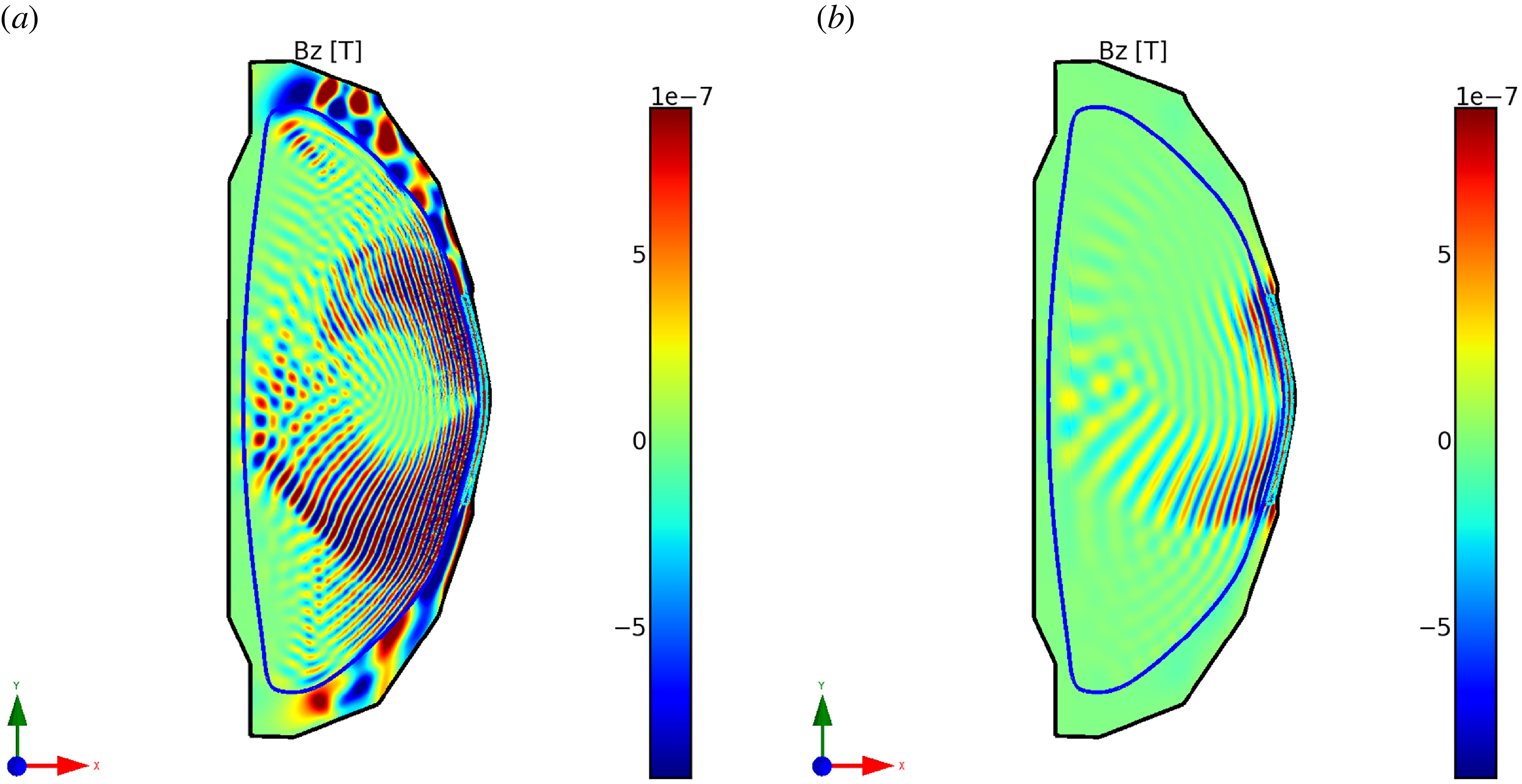
To demonstrate the impact of the higher magnetic-field operation at 1 T in NSTX-U on SOL mode coupling and propagation, figure 28 compares the HHFW magnetic field ( $B_\phi$
) between the
$B_\phi$
) between the $B_0$
= 0.5 T and
$B_0$
= 0.5 T and $B_0$
= 1.0 T using an NSTX-U equilibrium and realistic core density profiles. The experimental H-mode density profile (NSTX 130608) is adopted for the core density profile, as shown in figure 1 in Bertelli et al. (Reference Bertelli2014); density is nearly flat at
$B_0$
= 1.0 T using an NSTX-U equilibrium and realistic core density profiles. The experimental H-mode density profile (NSTX 130608) is adopted for the core density profile, as shown in figure 1 in Bertelli et al. (Reference Bertelli2014); density is nearly flat at ${\sim}3.7\times 10^{19}\,\mathrm{m}^{-3}$
with a local peaking at the pedestal top (
${\sim}3.7\times 10^{19}\,\mathrm{m}^{-3}$
with a local peaking at the pedestal top ( ${\sim}4\times 10^{19} \,\mathrm{m}^{-3}$
) due to carbon impurities. The SOL density is assumed to remain at
${\sim}4\times 10^{19} \,\mathrm{m}^{-3}$
) due to carbon impurities. The SOL density is assumed to remain at $3\times 10^{18}\,\mathrm{m}^{-3}$
. In this H-mode density profile, the density gradient at the LCFS remains steep, consistent with the step-like profile employed in the previous sections. In the
$3\times 10^{18}\,\mathrm{m}^{-3}$
. In this H-mode density profile, the density gradient at the LCFS remains steep, consistent with the step-like profile employed in the previous sections. In the $B_0$
= 0.5 T case, the local B-field magnitude at the antenna region is
$B_0$
= 0.5 T case, the local B-field magnitude at the antenna region is $B \approx$
0.44 T (
$B \approx$
0.44 T ( $B_\phi$
= 0.32 T and
$B_\phi$
= 0.32 T and $B_\theta$
= 0.3 T), while it is increased to
$B_\theta$
= 0.3 T), while it is increased to $B \approx$
0.7 T (
$B \approx$
0.7 T ( $B_\phi$
= 0.64 T and
$B_\phi$
= 0.64 T and $B_\theta$
= 0.3 T) in the
$B_\theta$
= 0.3 T) in the $B_0$
= 1.0 T case. The input wave toroidal number is
$B_0$
= 1.0 T case. The input wave toroidal number is $N_\phi$
= 5. At
$N_\phi$
= 5. At $B_0$
= 0.5 T, the SOL mode is clearly supported outside the antenna poloidal extent, reaching the top and bottom of the plasma and perturbing the core wavefield coupling. In contrast, at the higher-field NSTX-U condition (1 T), the SOL mode is suppressed. In this case, wave coupling is dominated by direct core penetration rather than parasitic SOL transport. These results demonstrate that the underlying bounded-mode-propagation mechanism identified in the simplified models remains operative in the realistic NSTX-U configuration, while geometric effects associated with both toroidal symmetry and wall shaping play a critical role in determining the SOL waveguide propagation.
$B_0$
= 0.5 T, the SOL mode is clearly supported outside the antenna poloidal extent, reaching the top and bottom of the plasma and perturbing the core wavefield coupling. In contrast, at the higher-field NSTX-U condition (1 T), the SOL mode is suppressed. In this case, wave coupling is dominated by direct core penetration rather than parasitic SOL transport. These results demonstrate that the underlying bounded-mode-propagation mechanism identified in the simplified models remains operative in the realistic NSTX-U configuration, while geometric effects associated with both toroidal symmetry and wall shaping play a critical role in determining the SOL waveguide propagation.
6. Discussion and summary
The present work addresses the excitation and transport of the waveguide-like modes in the annular SOL in the HHFW regime. The homogeneous fast-wave right-hand density cutoff is necessary but, by itself, does not excite SOL propagation. Instead, a geometric condition determines the existence of the eigenmode structure. As long as the SOL width is wide enough to support a radial half-wavelength structure, the plasma response can select and resonantly amplify the resonant modes in the antenna spectrum. Such a propagating mode is a manifestation of the same bounded-mode physics that also governs annulus resonance. As compared with the previous 1-D eigenvalue analysis (Perkins et al. Reference Perkins, Hosea, Bertelli, Taylor and Wilson2016), several new features are observed. Even a small field pitch can introduce asymmetry in the mode structure, a departure from the 1-D result. The SOL power transported away from the antenna can be redirected into the core plasma. Further, the present results help clarify earlier full-wave simulations, as the simulation domains in those studies likely implicitly satisfied the geometric condition. The parametric dependence of the bounded-mode onset and propagation is consistent with the experimental observations (Hosea et al. Reference Hosea2008). In this work, SOL dissipation mechanisms are not considered; however, as mentioned in the previous section, these SOL-localised waves are expected to cause parasitic losses identified in the past work, such as ionisation, collisions, RF sheath rectification (Perkins et al. Reference Perkins, Hosea, Jaworski, Bell, Bertelli, Kramer, Roquemore, Taylor and Wilson2017b
), mode conversion to slow waves (Tierens et al. Reference Tierens, Bilato, Bertelli, Shiraiwa, Myra and Colas2022) and parametric decay instabilities (Wilson et al. Reference Wilson, Bernabei, Biewer, Diem, Hosea, LeBlanc, Phillips, Ryan and Swain2005). In this finite element modelling work, kinetic core absorption models are missing (Bertelli et al. Reference Bertelli, Shiraiwa, Tierens and Scotti2023; Migliore, Usoltseva & Wright Reference Migliore, Usoltseva and Wright2026; Shiraiwa et al. Reference Shiraiwa, Bertelli, Kim, Wright, Verstraeten and Lamalle2026). In this work, an artificial collisional loss is introduced in the plasma core to simulate a strong single-pass regime. In regimes with weak single-pass absorption, the impact of the SOL mode on global wave propagation needs to be assessed, where the SOL geometric mode may affect the resulting wavefield structure and the final power partitioning. As the NSTX-U magnetic field increases from 0.5 to 1.0 T, the single-pass electron absorption is expected to decrease due to the $1/B^3$
scaling (Porkolab Reference Porkolab1994), while ion cyclotron absorption is expected to increase. AORSA simulations (Bertelli, Ono & Jaeger Reference Bertelli, Ono and Jaeger2019) predict that the electron-heating regime can be accessed for sufficiently high toroidal mode number, particularly in the absence of fast ions.
$1/B^3$
scaling (Porkolab Reference Porkolab1994), while ion cyclotron absorption is expected to increase. AORSA simulations (Bertelli, Ono & Jaeger Reference Bertelli, Ono and Jaeger2019) predict that the electron-heating regime can be accessed for sufficiently high toroidal mode number, particularly in the absence of fast ions.
The present studies demonstrate a clear role of magnetic pitch in mode formation. The pitch angle on NSTX/NSTX-U can reach $\sim$
45
$\sim$
45 $^\circ$
, and, therefore, incorporating a realistic field configuration is crucial, in addition to the physical geometries of plasma and antennas. In particular, in the past 3-D modelling (Bertelli, Shiraiwa & Ono Reference Bertelli, Shiraiwa and Ono2022), resonant structures localised to the SOL have been observed, and their connection to the geometric mode reported here can be revisited with a realistic H-mode density profile (in that study, a parabolic density profile was used). The SOL mode identified here is not expected to produce a purely field-aligned wavefield (e.g. slow-wave behaviour), as the mode is found to have a dominant axial power flow in addition to a poloidal power component (Baek et al. Reference Baek, Bertelli, Bonoli, De-Levante-Rodriguez and Shiraiwa2026). Identifying such a structure in three dimensions could help understand/evaluate the role of this mode in the RF spiral formation. Also, incorporating the divertor SOL density profile, as was done in two dimensions (De Levante Rodriguez et al. Reference De Levante Rodriguez, Baek, Shiraiwa, Bertelli and Bonoli2025), will be important for properly accounting for the narrow, low-density SOL region and capturing the influence of high-m mode structures on wave coupling and propagation.
$^\circ$
, and, therefore, incorporating a realistic field configuration is crucial, in addition to the physical geometries of plasma and antennas. In particular, in the past 3-D modelling (Bertelli, Shiraiwa & Ono Reference Bertelli, Shiraiwa and Ono2022), resonant structures localised to the SOL have been observed, and their connection to the geometric mode reported here can be revisited with a realistic H-mode density profile (in that study, a parabolic density profile was used). The SOL mode identified here is not expected to produce a purely field-aligned wavefield (e.g. slow-wave behaviour), as the mode is found to have a dominant axial power flow in addition to a poloidal power component (Baek et al. Reference Baek, Bertelli, Bonoli, De-Levante-Rodriguez and Shiraiwa2026). Identifying such a structure in three dimensions could help understand/evaluate the role of this mode in the RF spiral formation. Also, incorporating the divertor SOL density profile, as was done in two dimensions (De Levante Rodriguez et al. Reference De Levante Rodriguez, Baek, Shiraiwa, Bertelli and Bonoli2025), will be important for properly accounting for the narrow, low-density SOL region and capturing the influence of high-m mode structures on wave coupling and propagation.
In upcoming NSTX-U experiments, it remains to test the validity of the outer-wall PEC assumption and the role of the density gradient, as the details of the density profiles will matter for bounded-mode propagation. The RF wavefield measurements in the divertor SOL can yield critical wavefield data. One control parameter is the outer gap, but controlling it to reduce the SOL gap may not be practical due to interactions between neutral beam ions and the HHFW antenna. In previous experiments, a minimum outer gap of $\sim$
7 cm was required to prevent excessive heat loads to the antenna limiter (Hosea Reference Hosea2015). Therefore, parametric control of density and field will be needed. Based on this and previous studies (Hosea et al. Reference Hosea2008; Bertelli et al. Reference Bertelli, Shiraiwa and Ono2022), a higher-field operation on NSTX-U, up to 1 T, at a higher plasma current, up to 2 MA, is expected to provide a favourable SOL condition that suppresses geometric SOL coupling. The high-field operation will also raise the fast-wave right-hand cutoff density (threshold for fast-wave propagation), while lengthening the wave
$\sim$
7 cm was required to prevent excessive heat loads to the antenna limiter (Hosea Reference Hosea2015). Therefore, parametric control of density and field will be needed. Based on this and previous studies (Hosea et al. Reference Hosea2008; Bertelli et al. Reference Bertelli, Shiraiwa and Ono2022), a higher-field operation on NSTX-U, up to 1 T, at a higher plasma current, up to 2 MA, is expected to provide a favourable SOL condition that suppresses geometric SOL coupling. The high-field operation will also raise the fast-wave right-hand cutoff density (threshold for fast-wave propagation), while lengthening the wave $\lambda _\perp$
. Higher current (or lower Greenwald fraction) operation, along with wall conditioning, will help maintain the SOL density at a lower level. Density gradient can be another control parameter.
$\lambda _\perp$
. Higher current (or lower Greenwald fraction) operation, along with wall conditioning, will help maintain the SOL density at a lower level. Density gradient can be another control parameter.
Compared with the HHFW regime, a SOL geometric fit is not readily satisfied in low-harmonic ICRF scenarios, unless the field is lowered. For example, a low-field operation on ITER ( $B_0$
= 2.65 T) (Helou et al. Reference Helou2025) will result in a shorter perpendicular wavelength than that in the standard field (
$B_0$
= 2.65 T) (Helou et al. Reference Helou2025) will result in a shorter perpendicular wavelength than that in the standard field ( $B_0$
= 5.3 T). A nominal distance from the LCFS and the antenna is
$B_0$
= 5.3 T). A nominal distance from the LCFS and the antenna is $\sim$
20 cm, and the geometric condition could be satisfied if the phasing is low enough and the density remains high enough across the SOL (e.g.
$\sim$
20 cm, and the geometric condition could be satisfied if the phasing is low enough and the density remains high enough across the SOL (e.g. $\lambda _\perp /2 \approx 20\,\mathrm{cm}$
for
$\lambda _\perp /2 \approx 20\,\mathrm{cm}$
for $k_\parallel = 4\,\mathrm{m}^{-1}$
at
$k_\parallel = 4\,\mathrm{m}^{-1}$
at $n_{e,SOL} = 5\times 10^{18}\,\mathrm{m}^{-3}$
and
$n_{e,SOL} = 5\times 10^{18}\,\mathrm{m}^{-3}$
and $B_{\textit{SOL}} = 2$
T). Meanwhile, it is well known that ICRF waves can exhibit a global resonant response between the antenna and the ion–ion hybrid layer in the plasma core, with a clear increase in antenna loading in experiments and modelling (Ogawa et al. Reference Ogawa1991; Edlund et al. Reference Edlund, Bonoli, Porkolab and Wukitch2015). In addition, fast waves in the ICRF (Messiaen et al. Reference Messiaen, Koch, Bhatnagar, Vandenplas and Weynants1984) and in the lower hybrid range of frequencies (Pinsker & Colestock Reference Pinsker and Colestock1992) can couple to vacuum coaxial modes when a vacuum gap is wide enough, satisfying
$B_{\textit{SOL}} = 2$
T). Meanwhile, it is well known that ICRF waves can exhibit a global resonant response between the antenna and the ion–ion hybrid layer in the plasma core, with a clear increase in antenna loading in experiments and modelling (Ogawa et al. Reference Ogawa1991; Edlund et al. Reference Edlund, Bonoli, Porkolab and Wukitch2015). In addition, fast waves in the ICRF (Messiaen et al. Reference Messiaen, Koch, Bhatnagar, Vandenplas and Weynants1984) and in the lower hybrid range of frequencies (Pinsker & Colestock Reference Pinsker and Colestock1992) can couple to vacuum coaxial modes when a vacuum gap is wide enough, satisfying $k_0 x_p \sim \pi$
, where
$k_0 x_p \sim \pi$
, where $k_0 = \omega /c$
is the vacuum wavenumber and
$k_0 = \omega /c$
is the vacuum wavenumber and $x_p$
is the vacuum gap. This fit condition in the vacuum region is geometrically analogous to the plasma-filled mode discussed here.
$x_p$
is the vacuum gap. This fit condition in the vacuum region is geometrically analogous to the plasma-filled mode discussed here.
In summary, this paper has discussed the onset of fast-wave propagation in the NSTX/NSTX-U SOL plasma as a bounded-waveguide mode, a spatial manifestation of a geometry-selected fast-wave eigenmode. The 2-D full-wave model describes mode excitation and propagation in the annular SOL, as well as the impact of the magnetic-field geometry on the eigenmode structure in an anisotropic plasma. In line with previous studies on annulus resonance and HHFW full-wave modelling, the parametric dependence of the mode-onset condition is consistent with the experimental trends. When the geometric condition is met, a large-amplitude wavefield can be trapped and guided by the SOL plasma and is expected to dissipate there, leading to a loss of HHFW core-heating efficiency. These results provide a unified view on past numerical observations on HHFW coupling and SOL propagation, offering insights for future experimental optimisation of HHFW scenario development.
Acknowledgements
This work was supported by the U.S. DoE awards, DESC0021120, and DE-AC02-05CH11231 using NERSC award FES-ERCAP0027700. This manuscript has been co-authored by Princeton University/Princeton Plasma Physics Laboratory under contract number DE-AC02-09CH11466 with the U.S. Department of Energy. The United States Government retains a non-exclusive, paid-up, irrevocable, world-wide licence to publish or reproduce the published form of this manuscript, or allow others to do so, for United States Government purpose(s).
Editor Troy Carter thanks the referees for their advice in evaluating this article.
Declaration of interests
The authors report no conflict of interest.
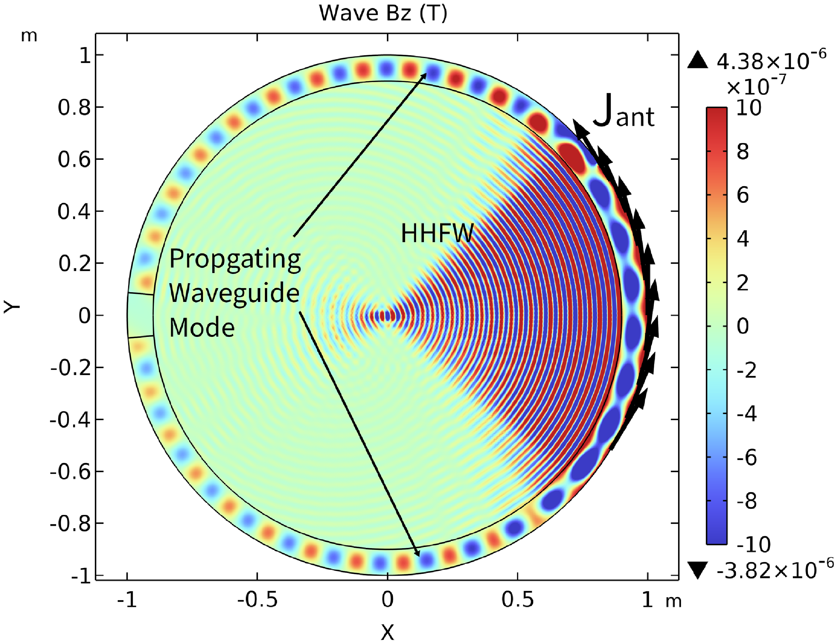
 ne,core
 3×10¹⁹m−3
 ne,SOL
 3×10¹⁸m−3
 B0
B0 α
α ∘
∘ |θ|⩽36∘
 Jant
Jant Bz=B∥
Bz=B∥ 175∘⩽θ⩽185∘
 σ
σ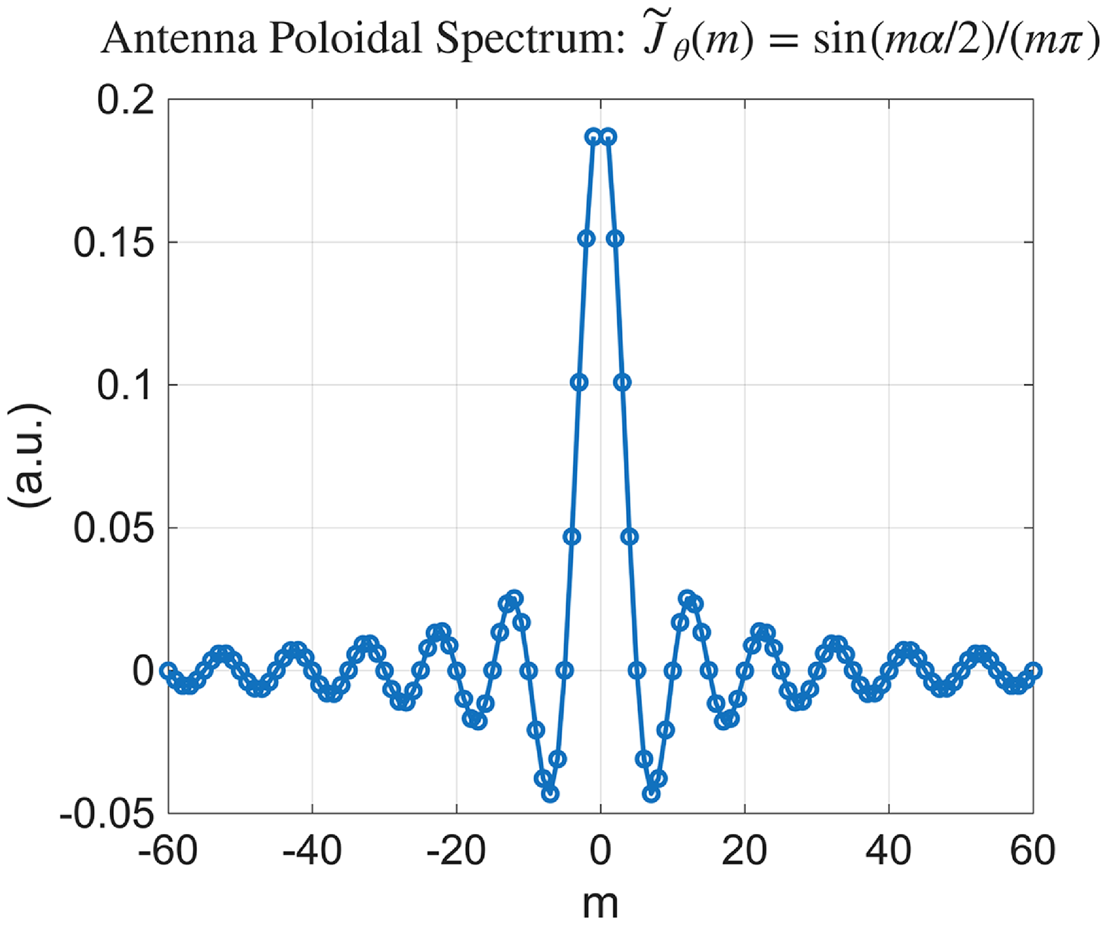
 α
α ∘
∘ J~θ(m)=sin(mα/2)/(mπ)
 m→
m→ J~θ=α/(2π)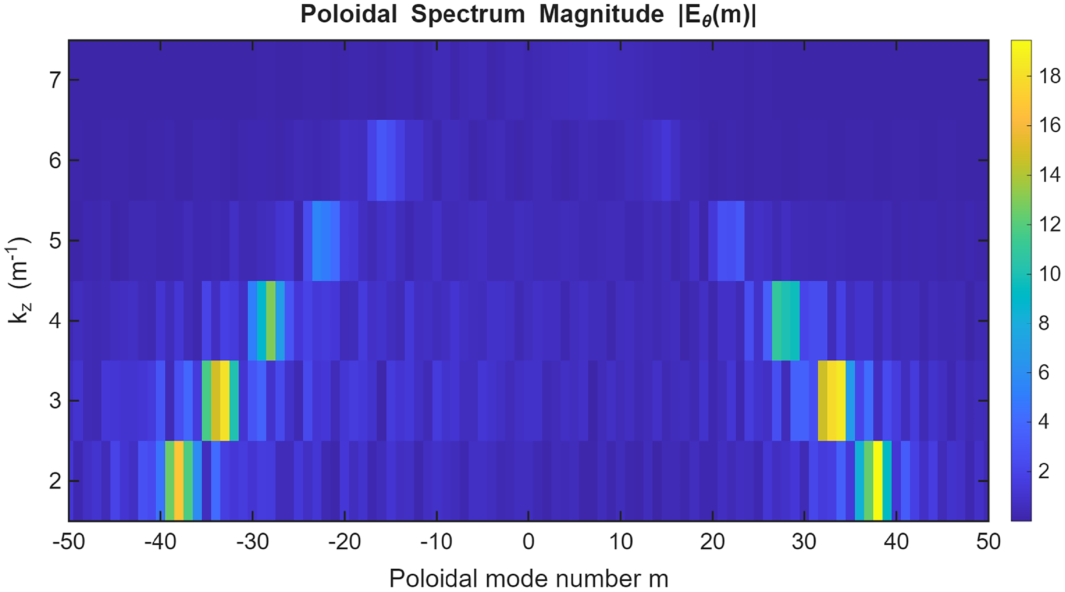
 Eθ
Eθ k∥
k∥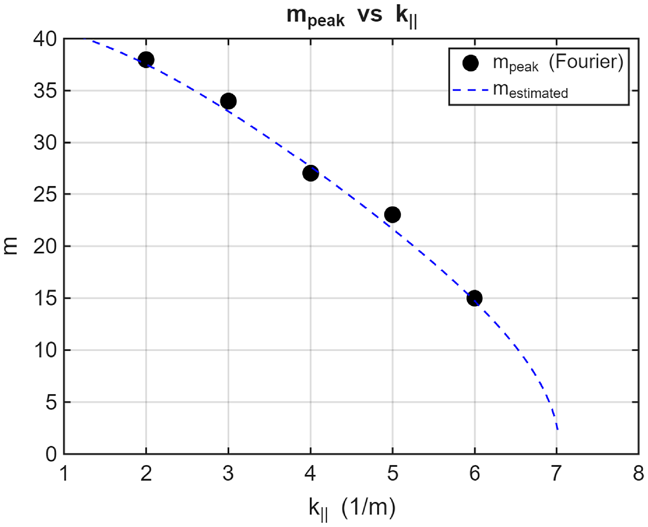
 mpeak
mpeak mestimated
 k∥=kz
k∥=kz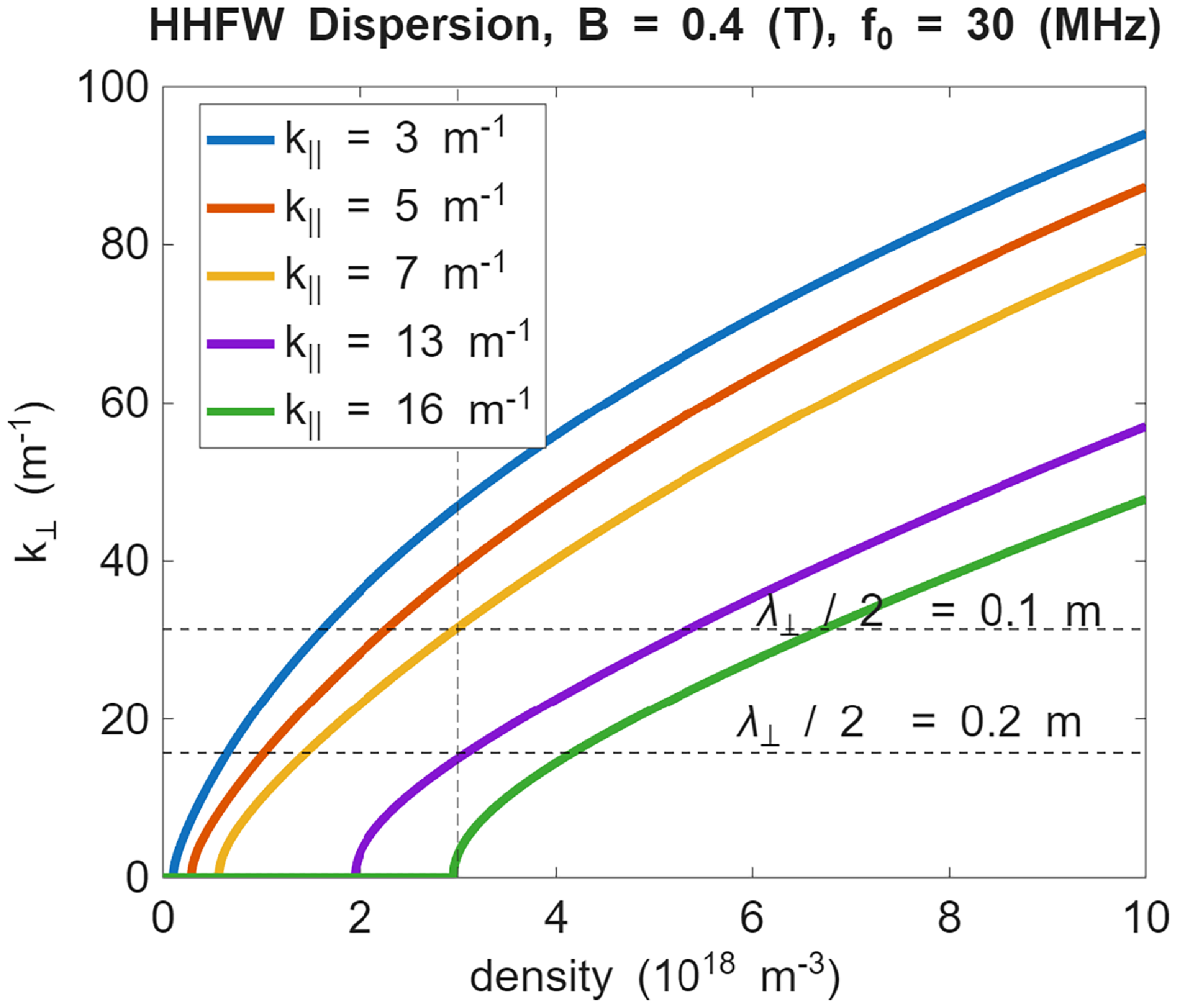
 k⊥
k⊥ k∥
k∥ B
B f0
f0 λ⊥/2
λ⊥/2 λ⊥/2
λ⊥/2 ne=3×10¹⁸m−1
 k∥=7
k∥=7 m−1
m−1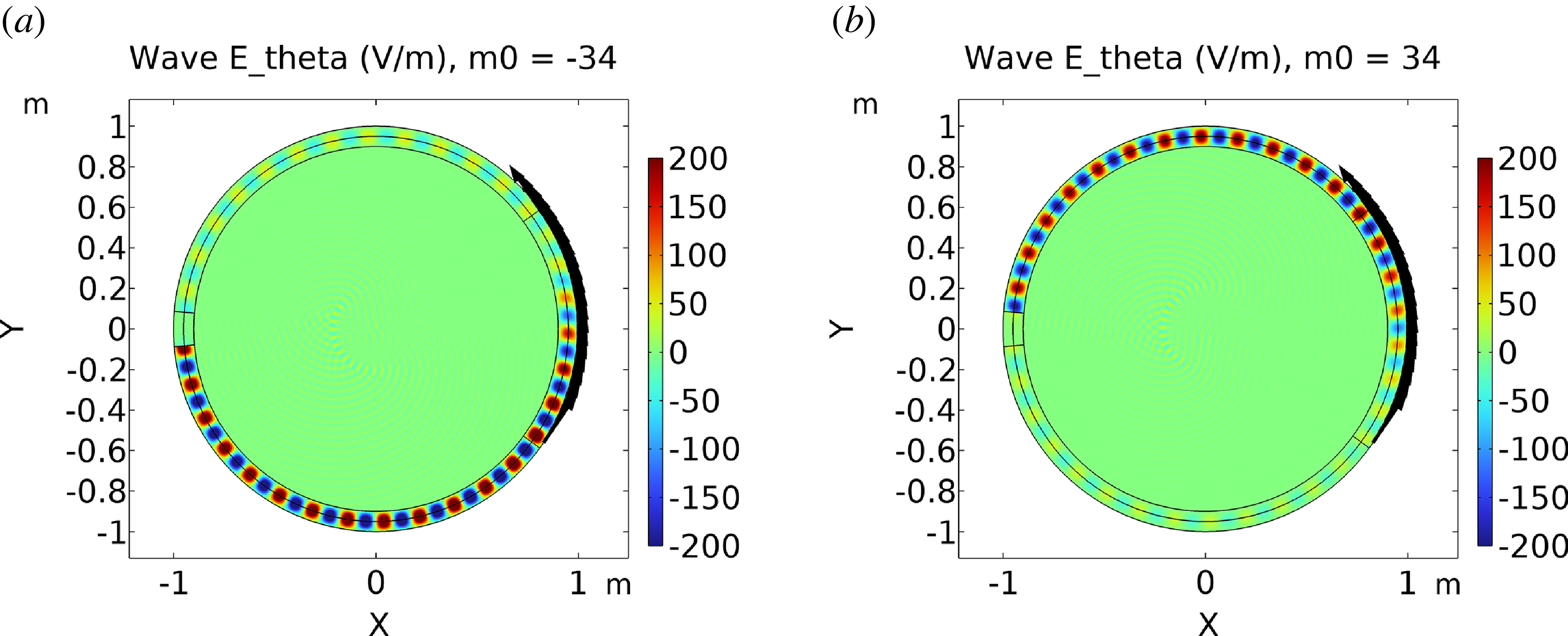
 Eθ
Eθ jθ=θ^exp(im0θ)
 θ^=−sinθx^+cosθy^
 m0
m0 m0
m0 kz
kz 3m−1
3m−1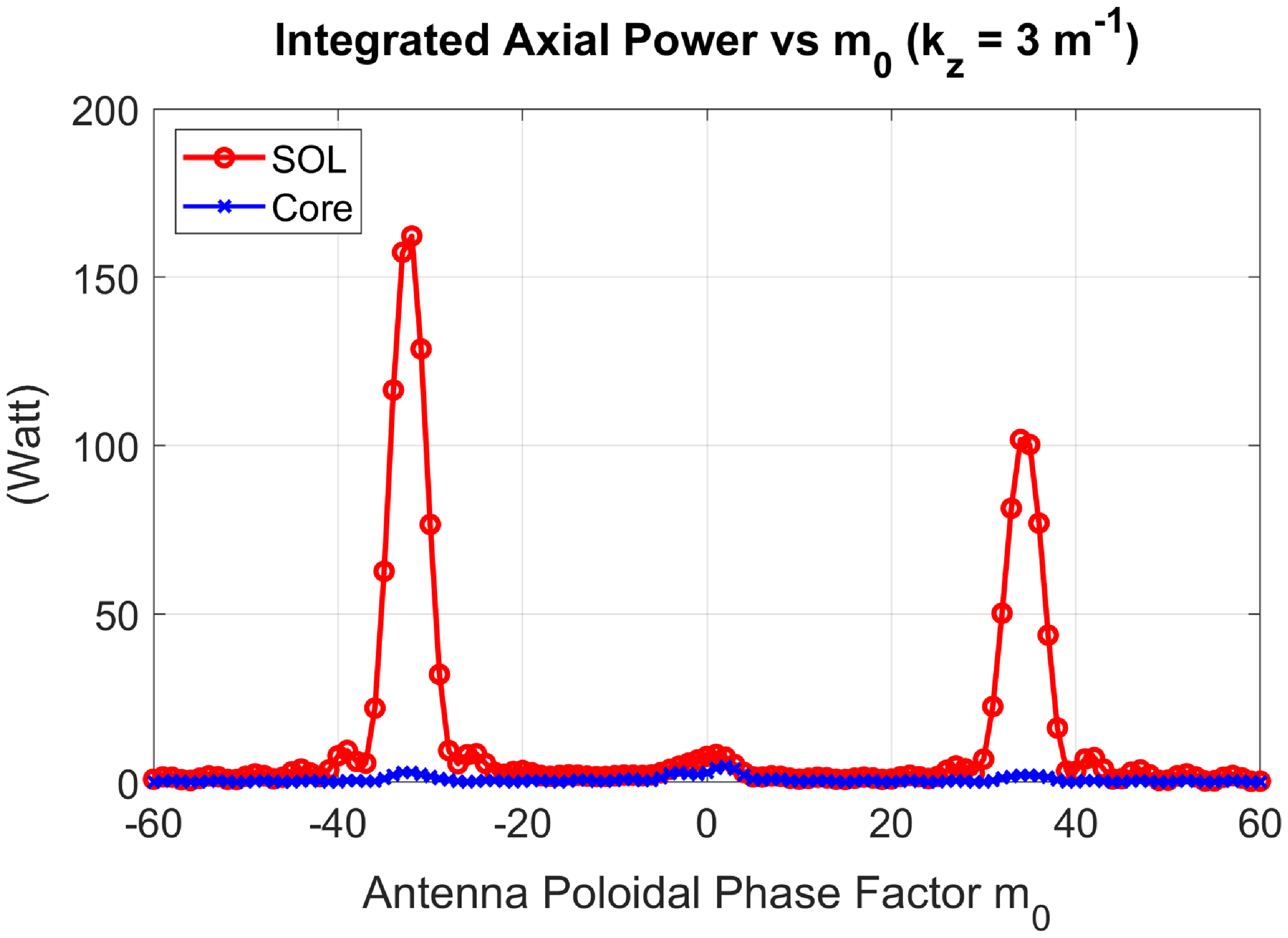
 Sz=(1/2)∫(ExHy∗−EyHx∗)dA
 m0
m0 kz
kz 3m−1
3m−1 B
B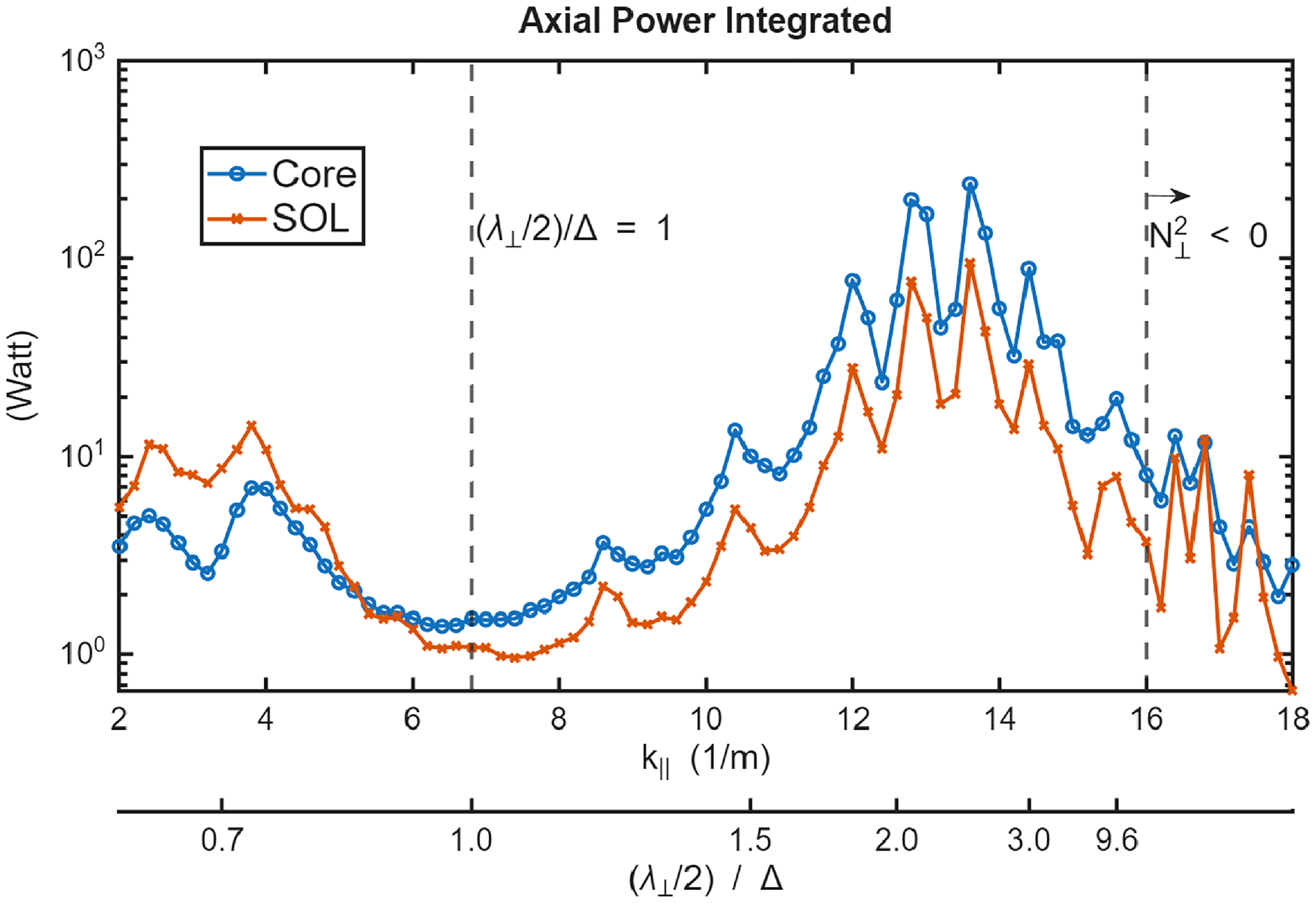
 k∥
k∥ k∥
k∥ (λ⊥/2)/Δ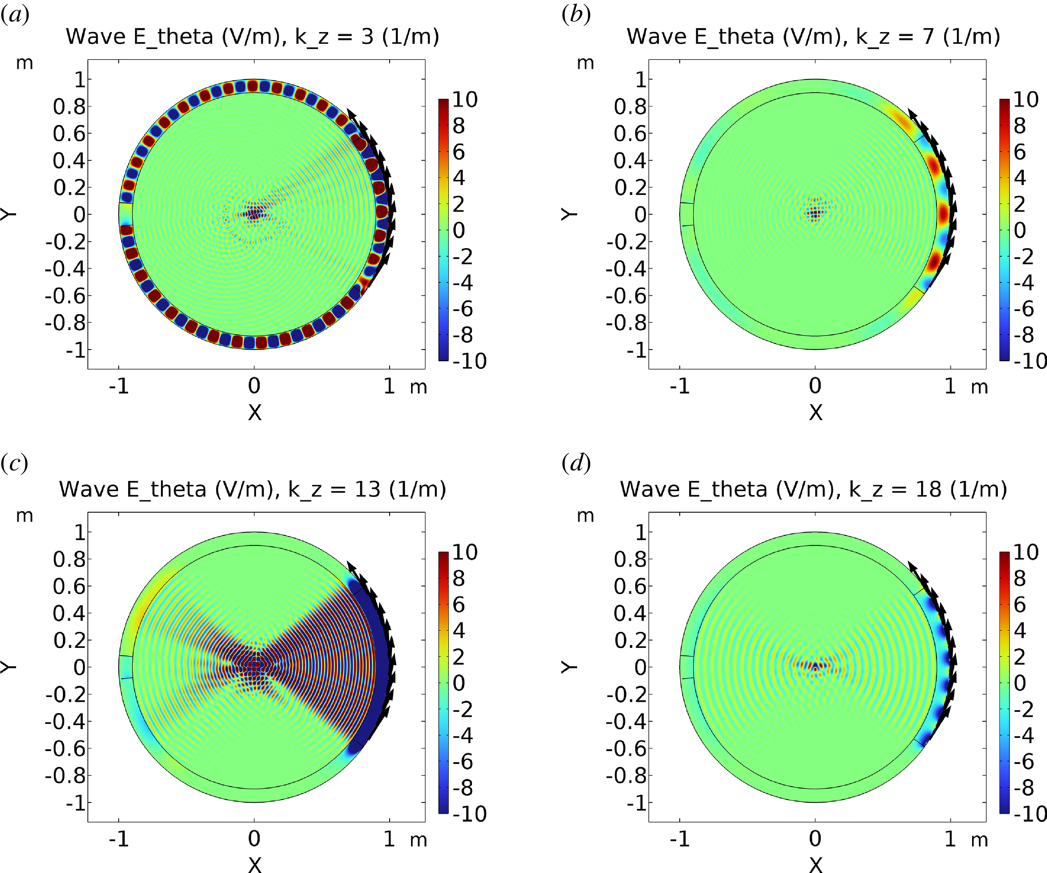
 Eθ
Eθ kz
kz m−1
m−1 m−1
m−1 m−1
m−1 m−1
m−1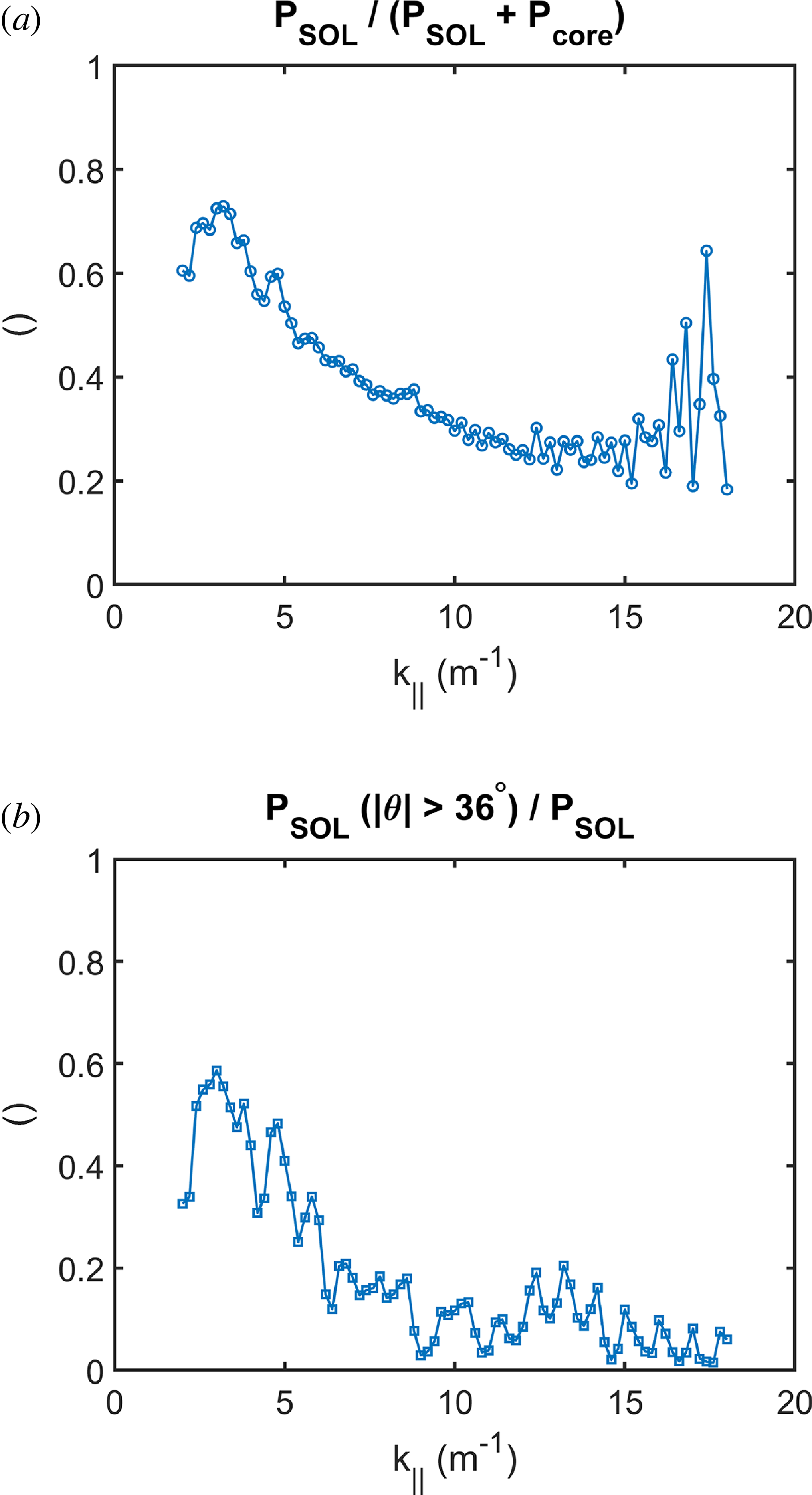
 k∥
k∥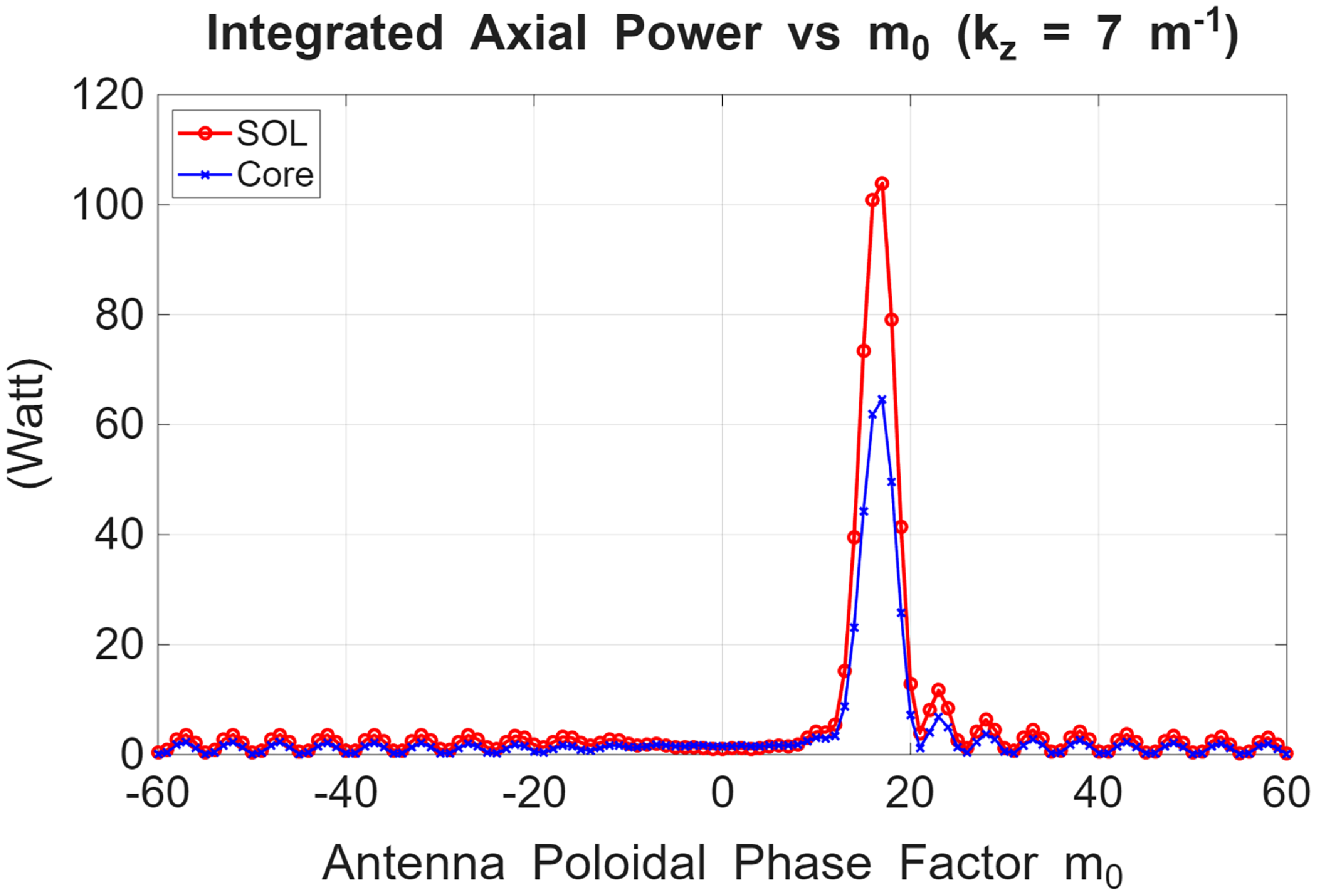
 Sz=(1/2)∫(ExHy∗−EyHx∗)dA
 m0
m0 jθ=θ^exp(im0θ)
 θ^=−sinθx^+cosθy^
 kz
kz 7m−1
7m−1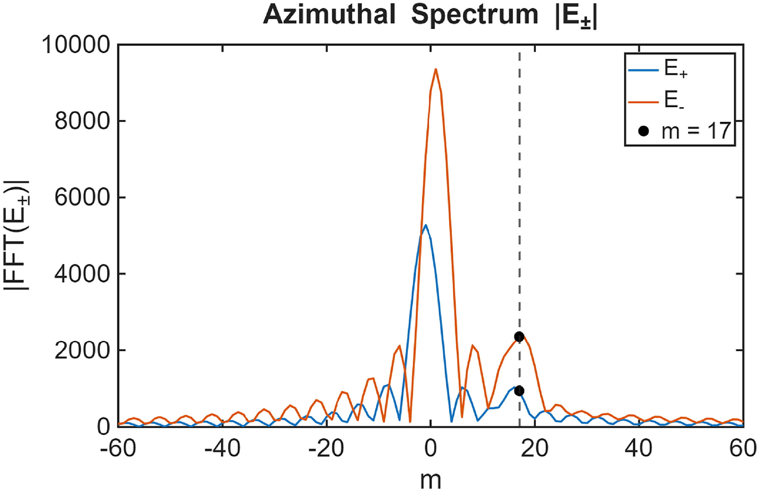
 E±
E± kz=7
kz=7 m−1
m−1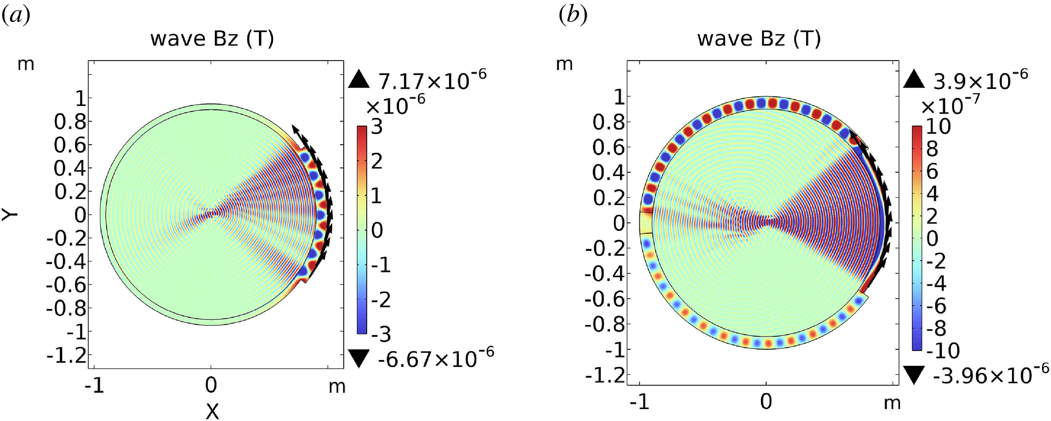
 kz
kz m−1
m−1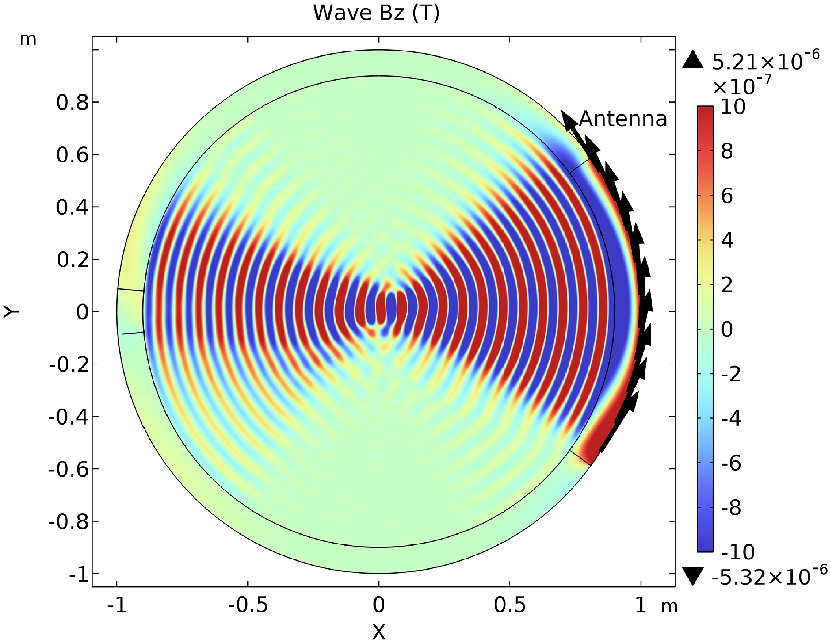
 kz
kz m−1
m−1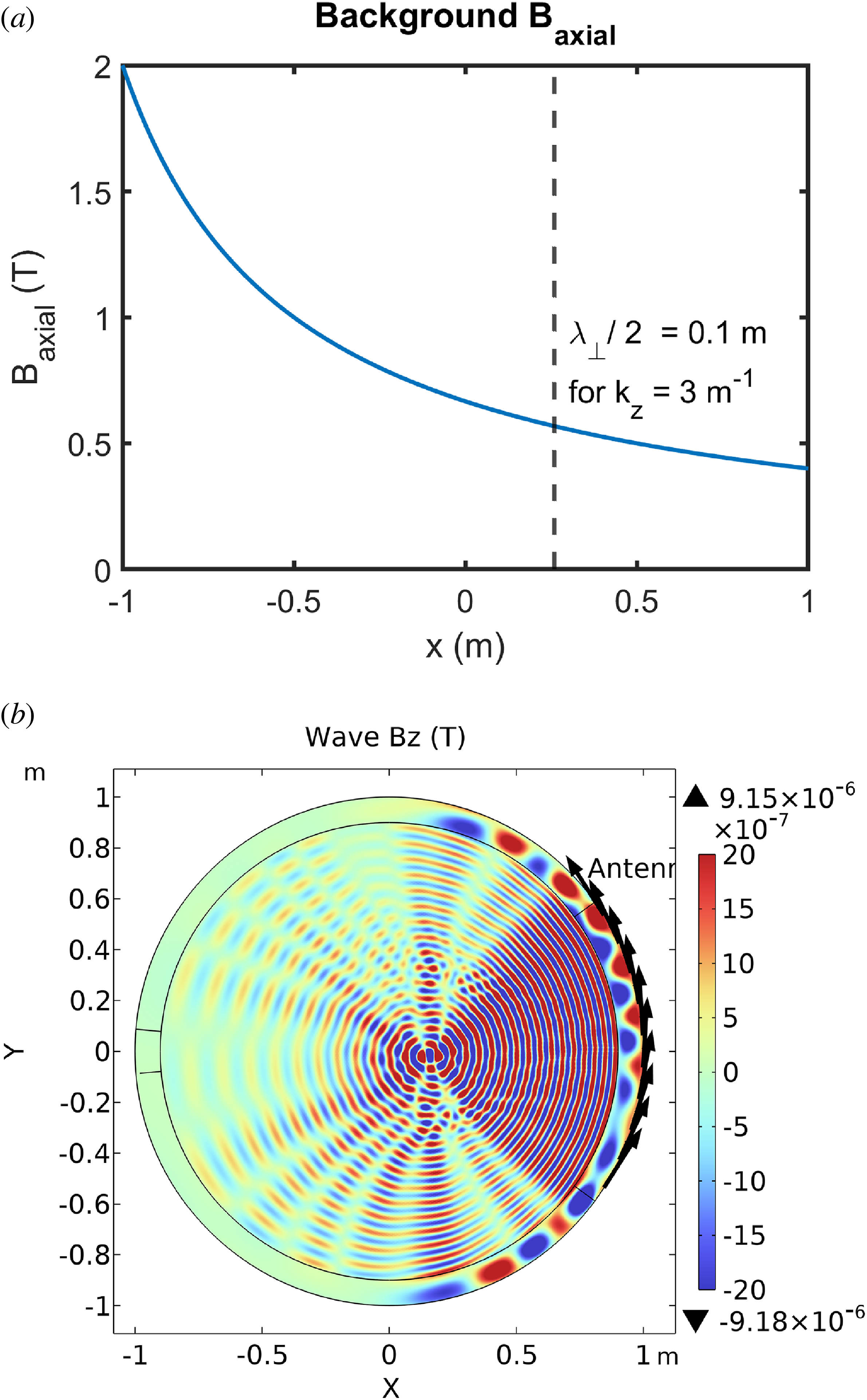
 kz
kz m−1
m−1 <
< >
> Bz
Bz ≈
≈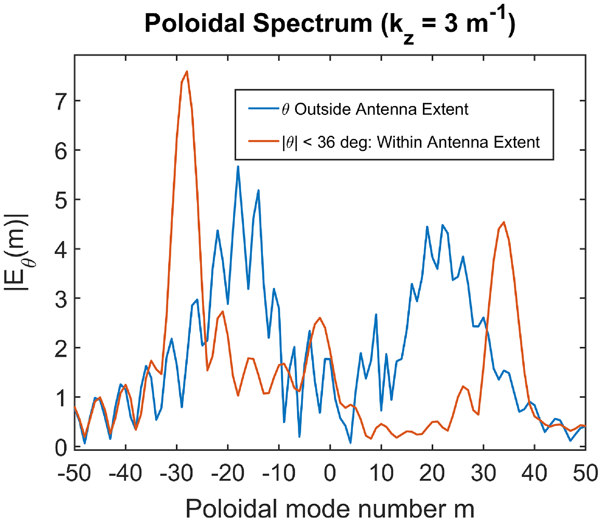
 Eθ
Eθ kz
kz m−1
m−1 kz
kz m−1
m−1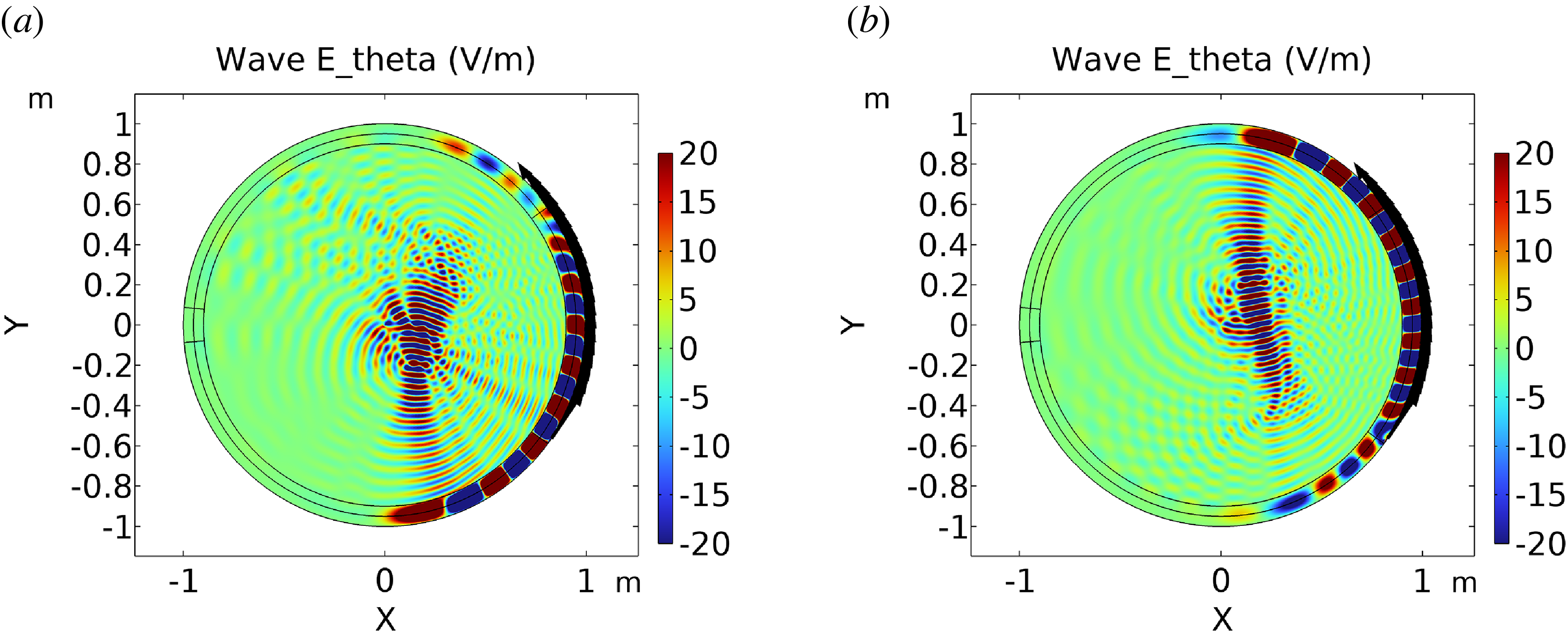
 Eθ
Eθ jθ=θ^exp(im0θ)
 m0
m0 m0
m0 kz
kz m−1
m−1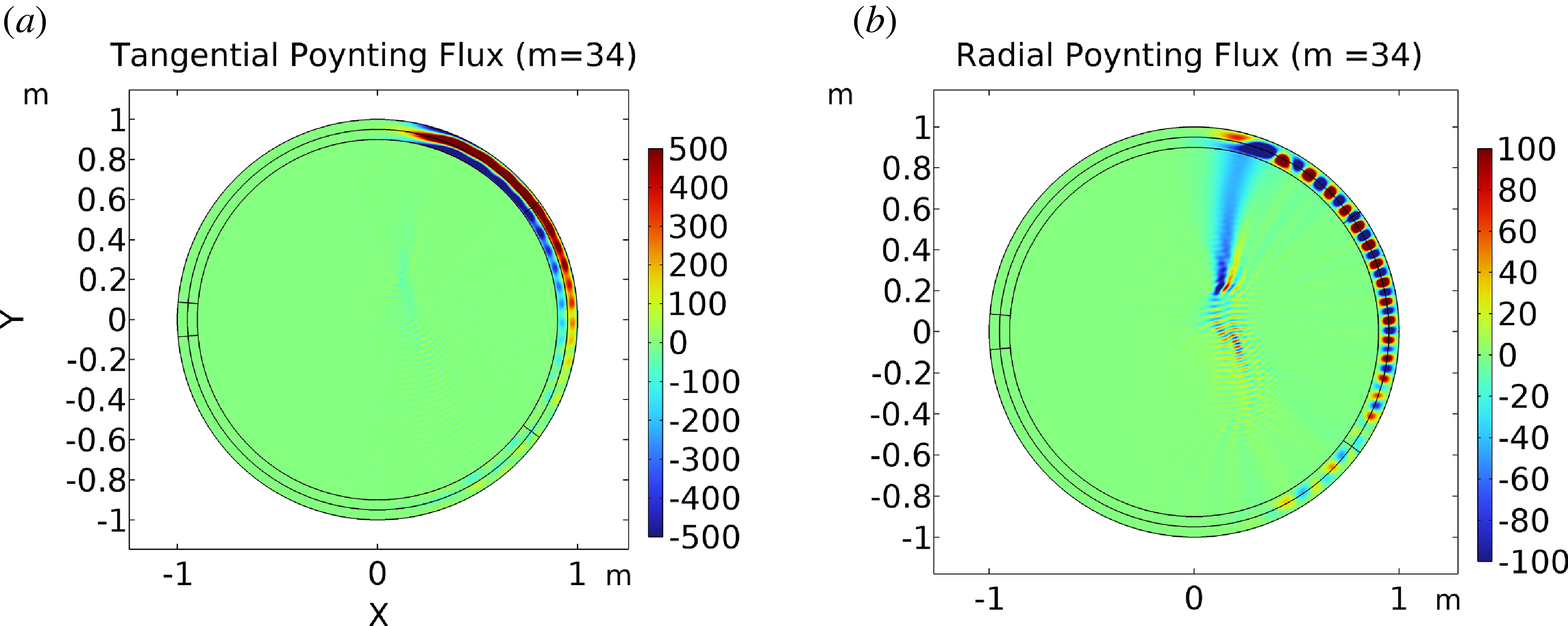
 m0
m0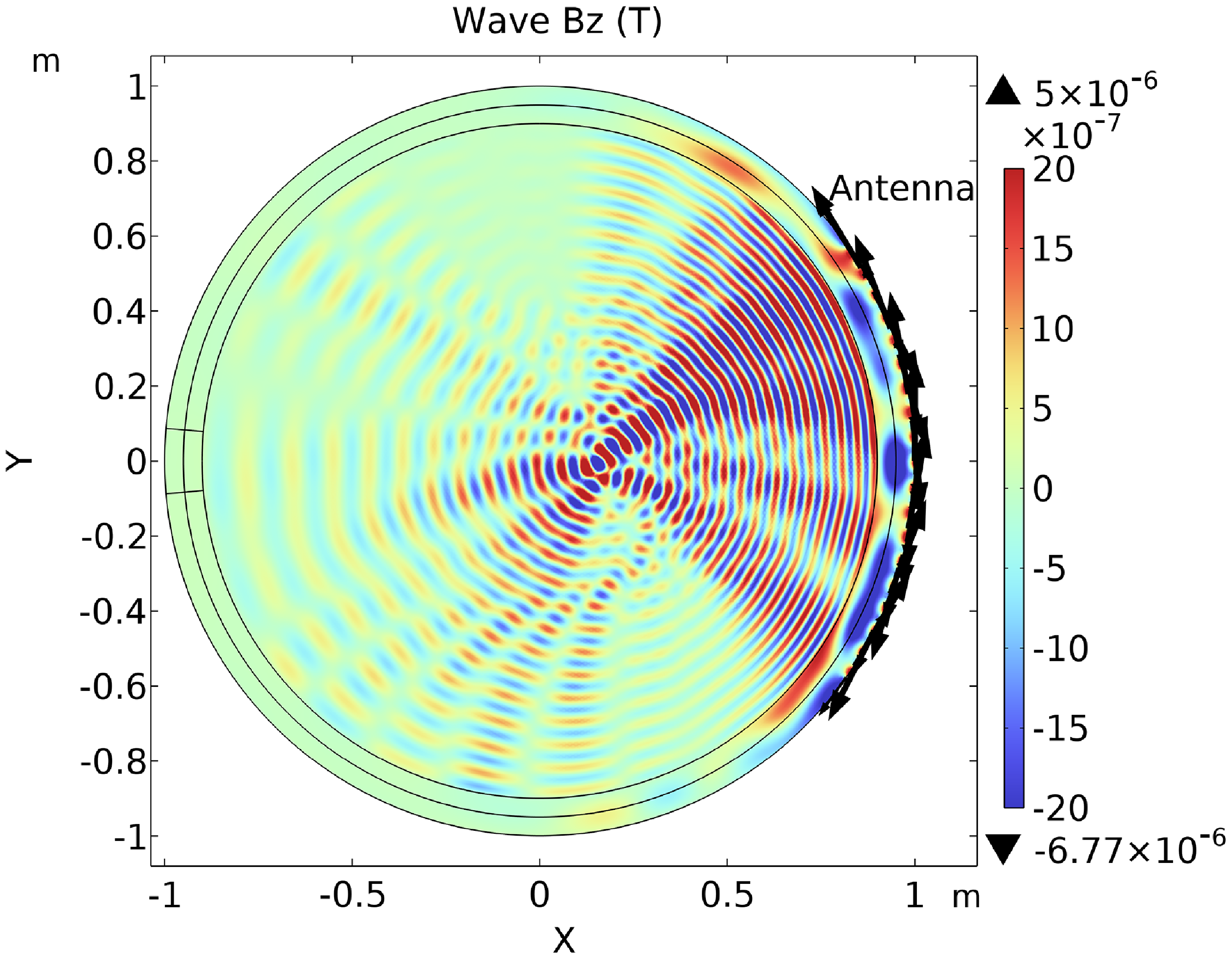
 Bz
Bz kz
kz m−1
m−1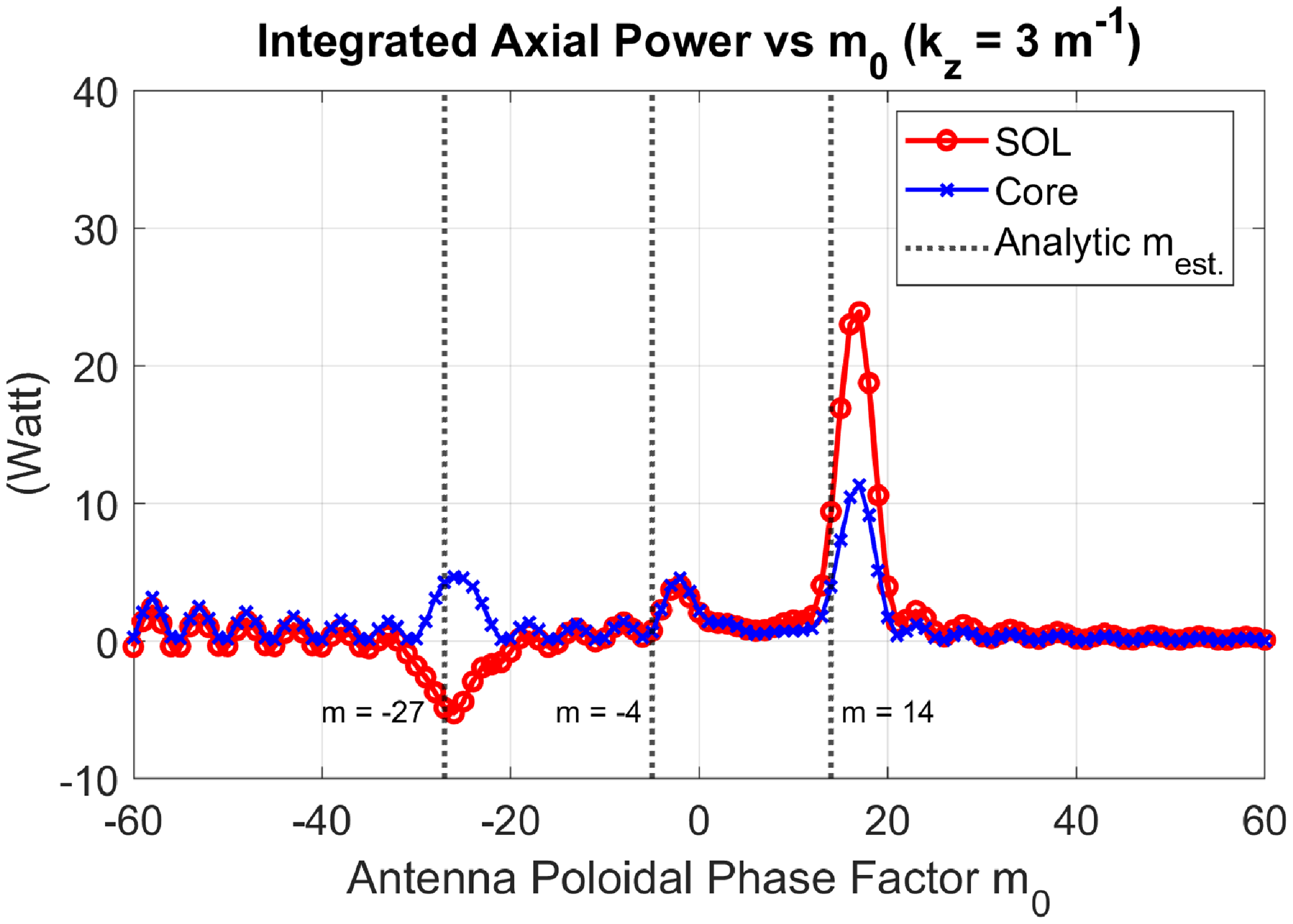
 m0
m0 exp(im0θ)
 kz
kz m−1
m−1 mest
mest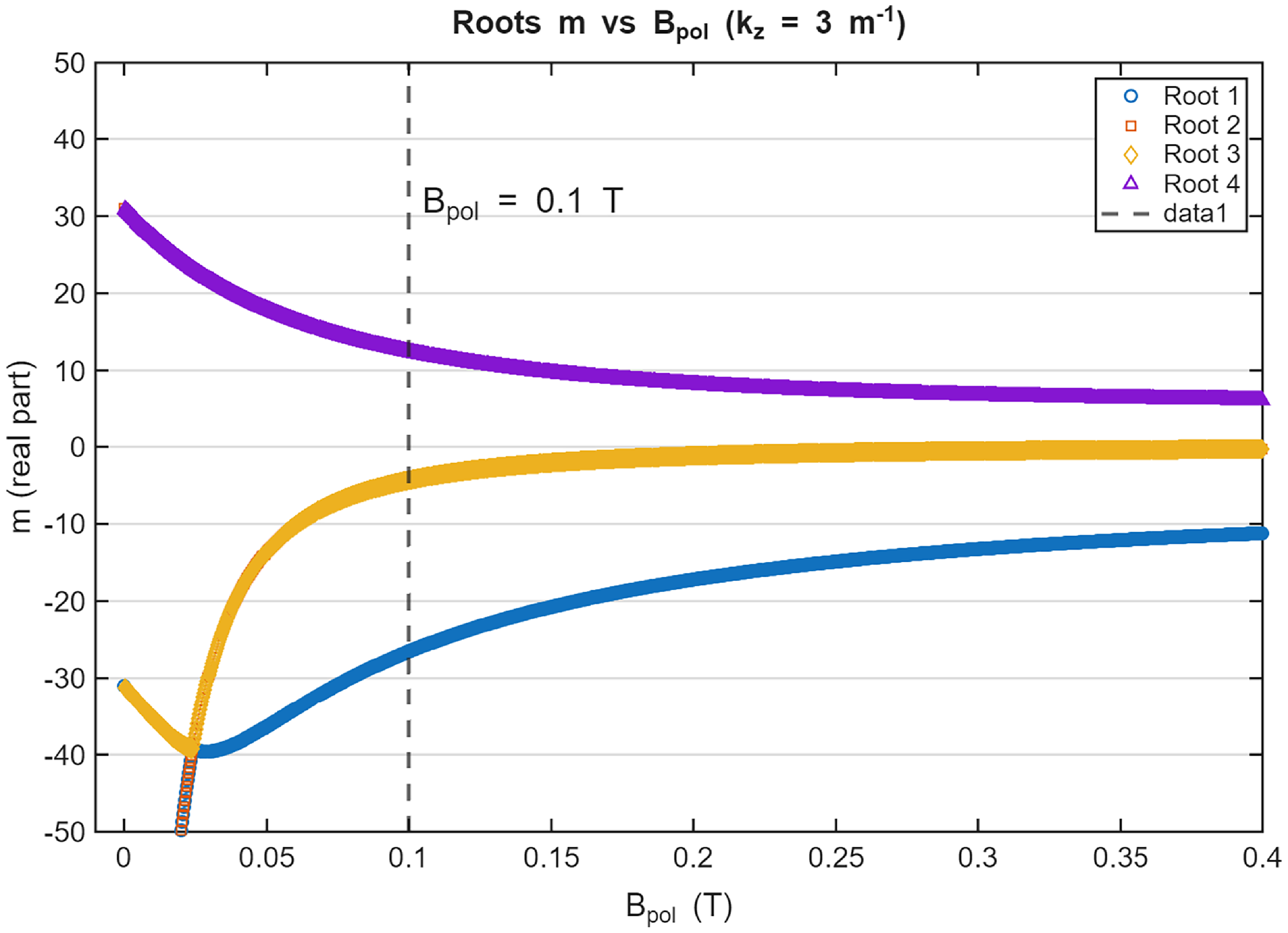
 Bθ
Bθ kz=3m−1
 Bz
Bz ne=3×10¹⁸m−3
 reff
reff kr=π/Δ
 Δ=0.1m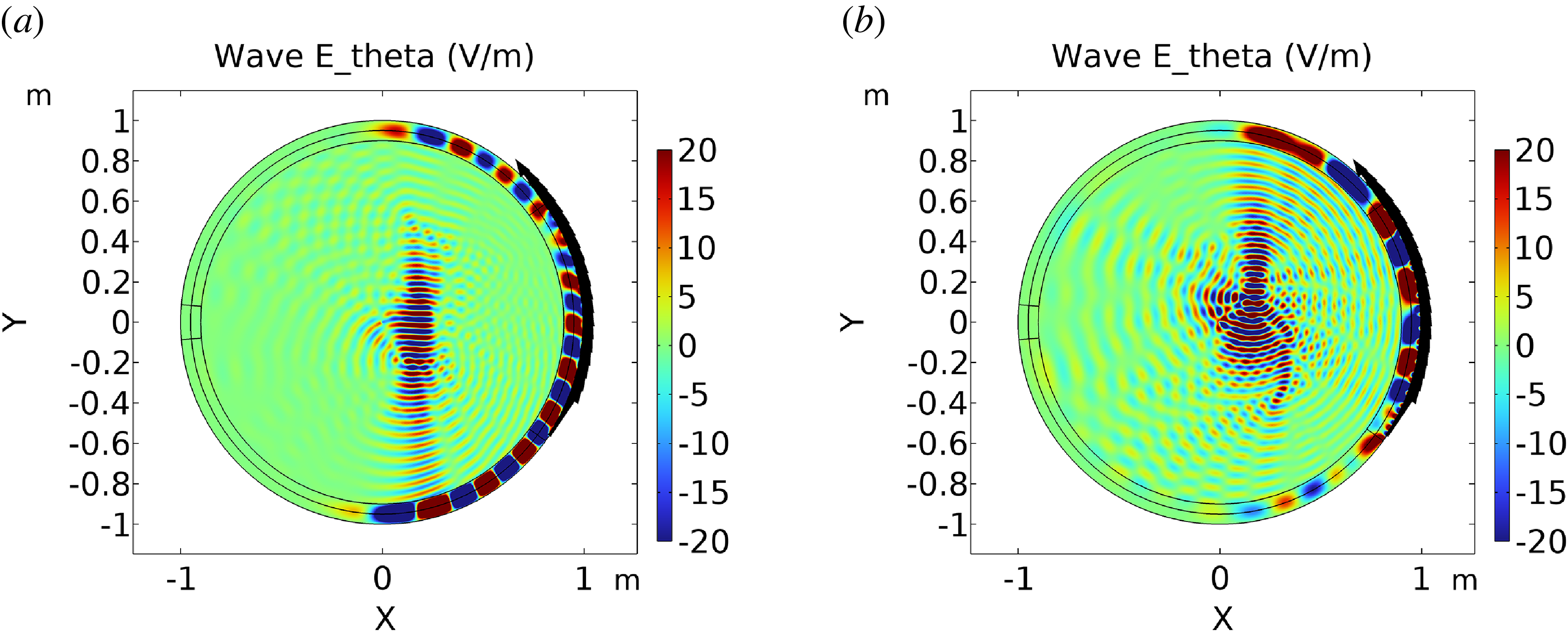
 Eθ
Eθ jθ=θ^exp(im0θ)
 θ^=−sinθx^+cosθy^
 m0
m0 m0
m0 kz
kz m−1
m−1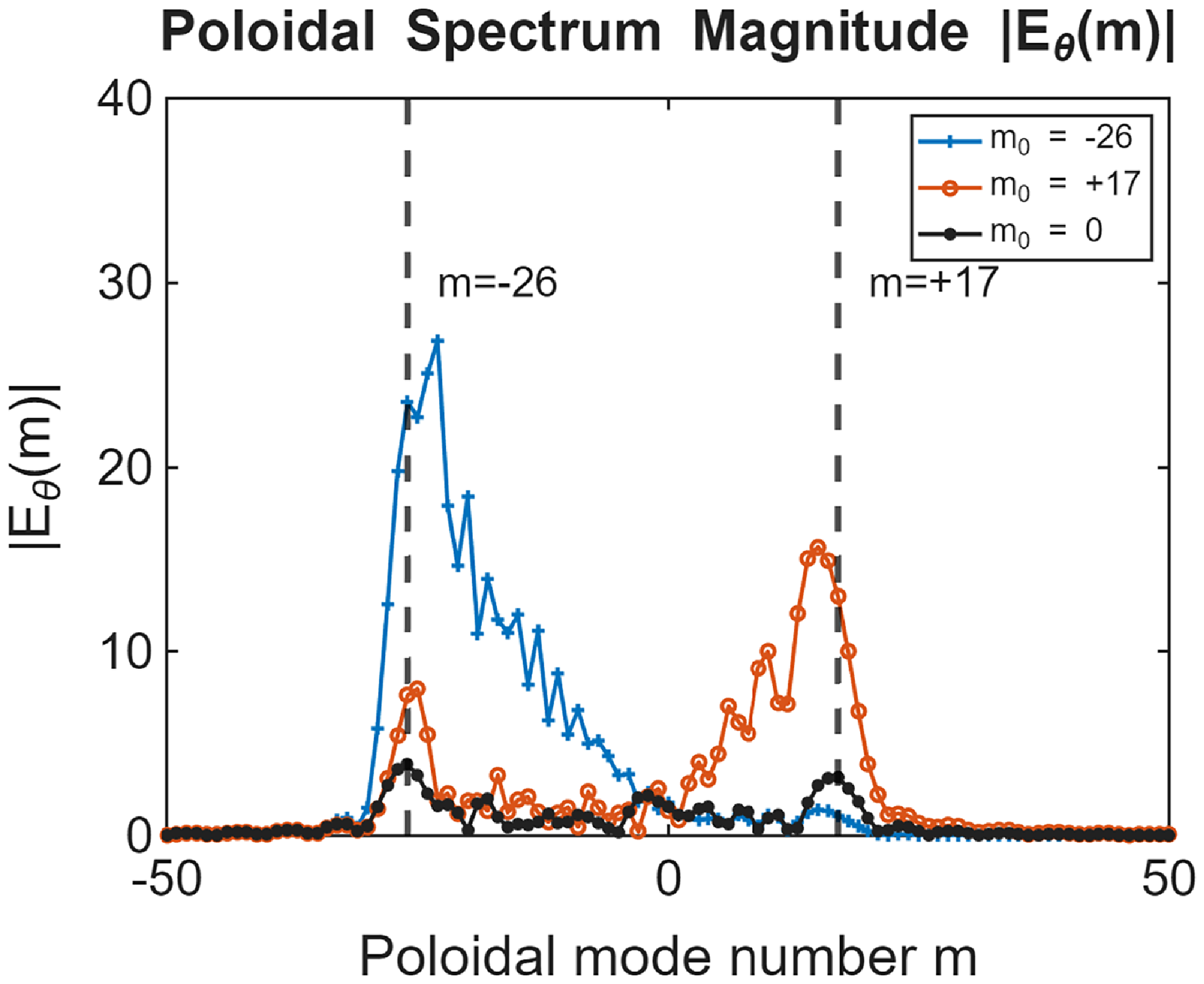
 m0
m0 m0
m0 m0=17
m0=17 m≈−26
m≈−26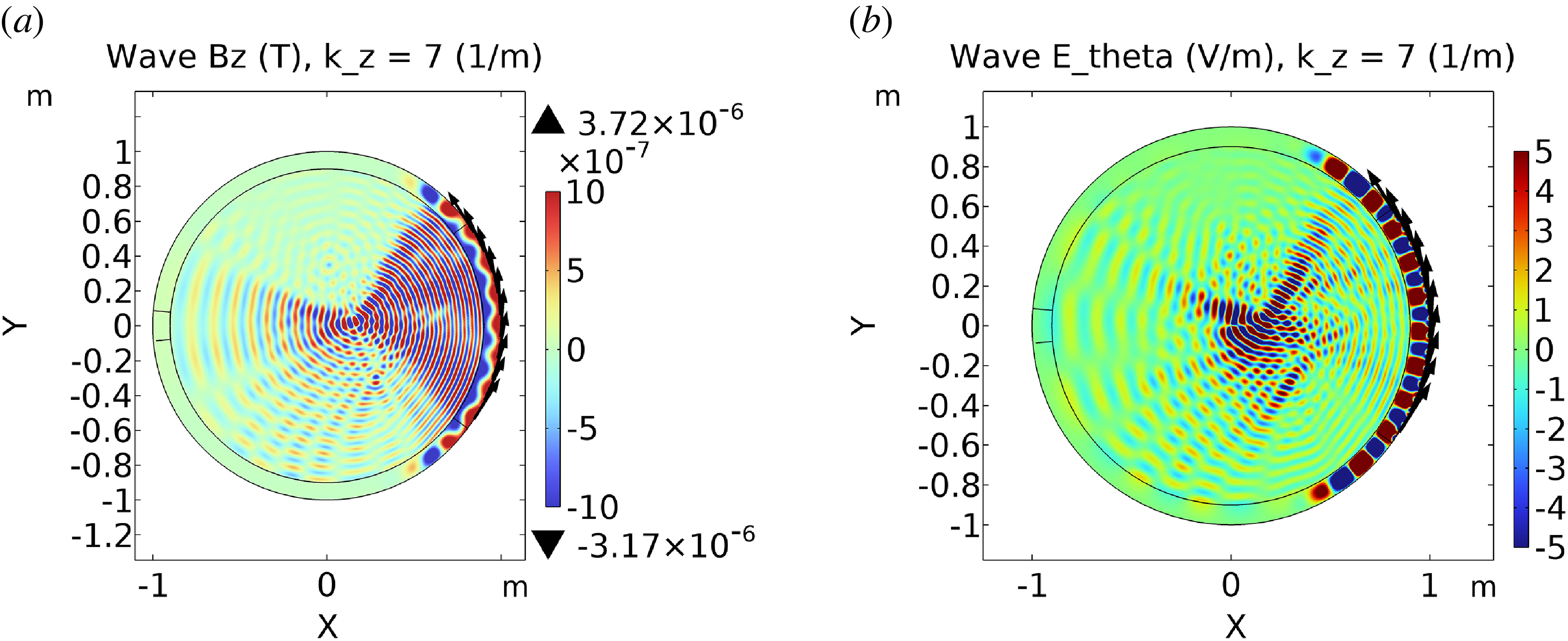
 Bz
Bz Eθ
Eθ kz
kz m−1
m−1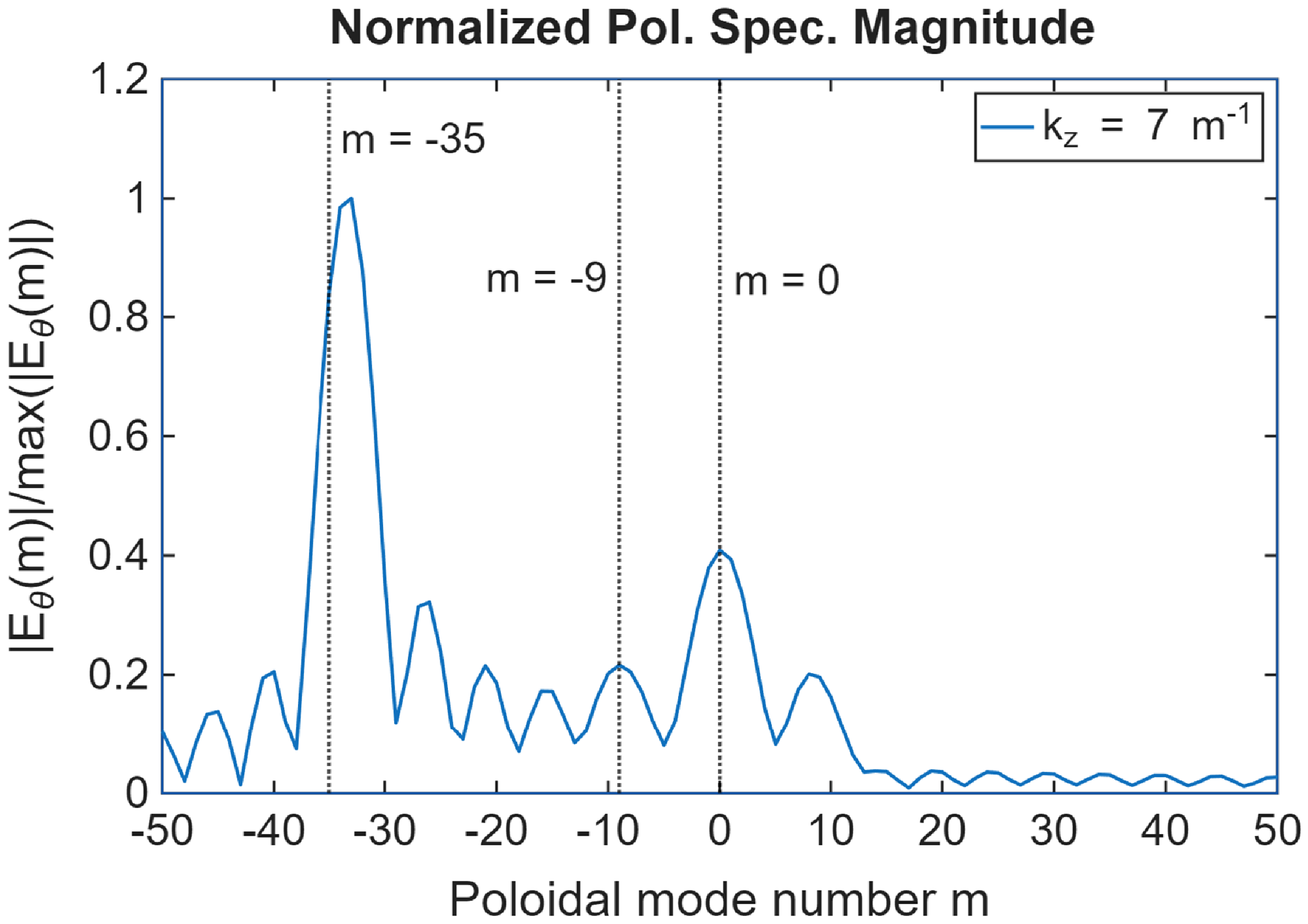
 kz
kz m−1
m−1 m0
m0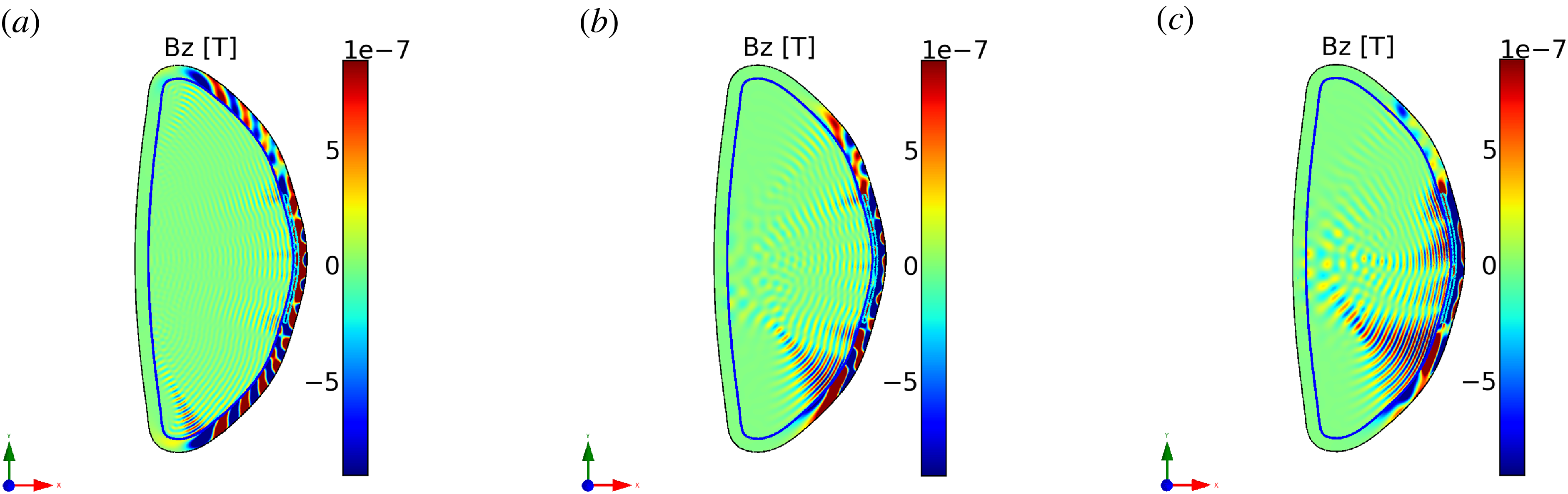
 Bθ,max
 Nϕ
Nϕ kϕ=Nϕ/Rant≈3.24m−1
 Rant
Rant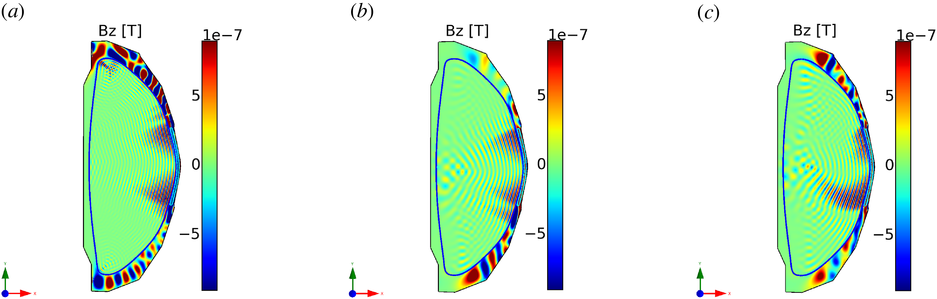
 Bθ,max
 Nϕ
Nϕ kϕ=Nϕ/Rant≈3.24m−1
 Rant
Rant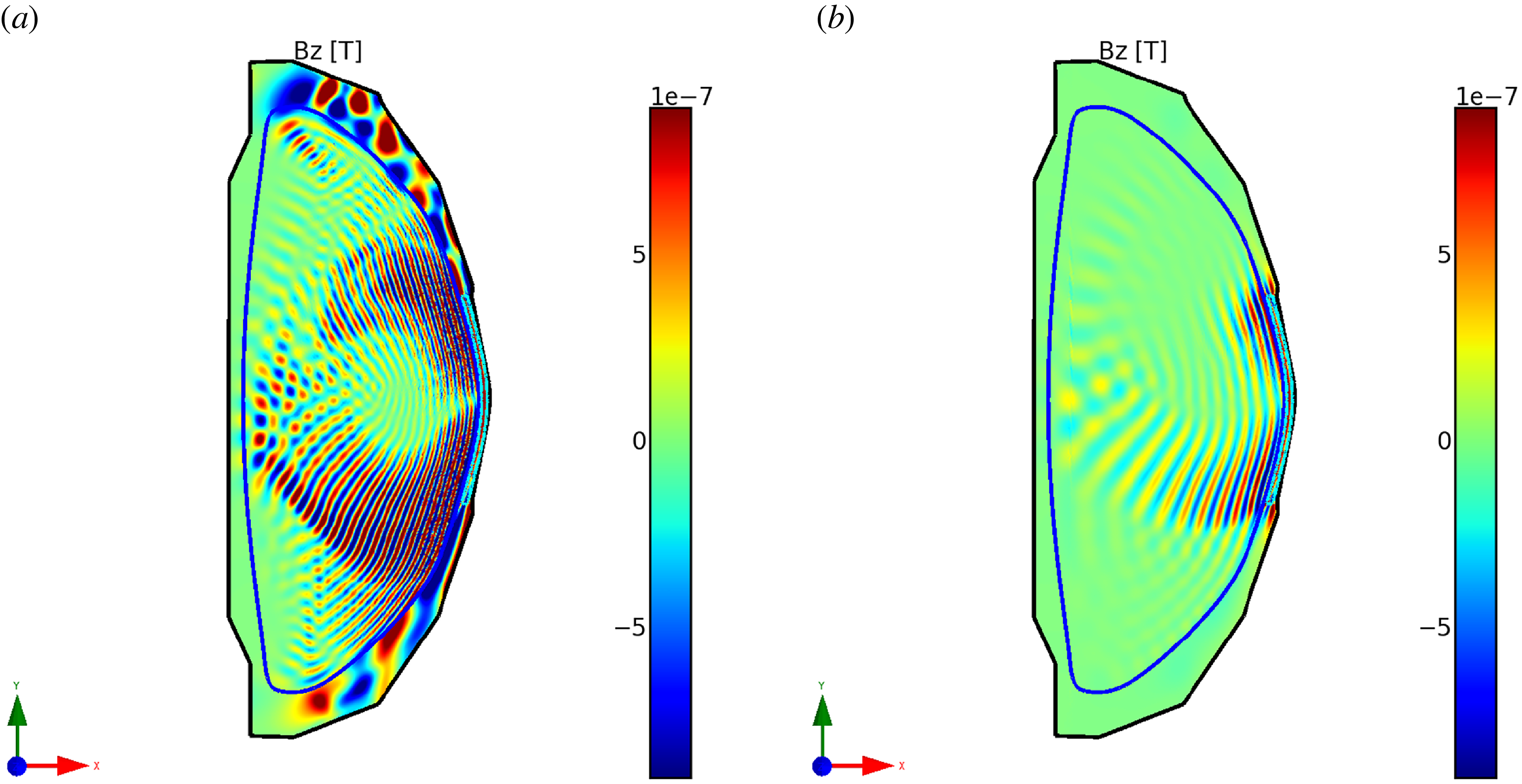
 B0
B0 B0
B0
 Open access

