


1 Introduction
High-average-power and high-energy lasers play an important role in many fields of current scientific research and industrial processing[ Reference Betti and Hurricane 1 – Reference Rus, Bakule, Kramer, Naylon, Thoma, Fibrich, Green, Lagron, Antipenkov, Bartoníček, Batysta, Baše, Boge, Buck, Cupal, Drouin, Ďurák, Himmel, Havlíček, Homer, Honsa, Horáček, Hríbek, Hubáček, Hubka, Kalinchenko, Kasl, Indra, Korous, Košelja, Koubíková, Laub, Mazanec, Meadows, Novák, Peceli, Polan, Snopek, Šobr, Trojek, Tykalewicz, Velpula, Verhagen, Vyhlídka, Weiss, Haefner, Bayramian, Betts, Erlandson, Jarboe, Johnson, Horner, Kim, Koh, Marshall, Mason, Sistrunk, Smith, Spinka, Stanley, Stolz, Suratwala, Telford, Ditmire, Gaul, Donovan, Frederickson, Friedman, Hammond, Hidinger, Chériaux, Jochmann, Kepler, Malato, Martinez, Metzger, Schultze, Mason, Ertel, Lintern, Edwards, Hernandez-Gomez and Collier 3 ]. Due to the high energies in a pulse, large-aperture amplifiers are necessary. However, the amplification of a large-aperture high-power high-energy laser beam in multistage amplifier systems often suffers from beam profile inhomogeneities caused by a nonuniform gain[ Reference Dorrer and Zuegel 4 , Reference Zhao, Yu, Li, Huang, Ma, Tang and Fan 5 ]. There is great effort to either pre-compensate or improve the spatial beam profile or wavefront in order to avoid optics damage in the amplifiers and to achieve the most uniform output. For this purpose, various types of spatial light modulator (SLM)-based beam shapers have been deployed at several laser facilities in their laser systems[ Reference Awwal, Orth, Tse, Matone, Paul, Hardy, Brunton, Hermann, Yang, DiNicola, Rever, Dixit and Heebner 6 – Reference Zhao, Liang, Li, Zong, Tang, Zhao, Wang, Li, Zeng, Xia, Chen, Chen, Zheng, Wei and Zhu 11 ] or in test experiments[ Reference Bagnoud and Zuegel 12 – Reference Maxson, Bartnik and Bazarov 15 ].
SLMs allow one to shape the incident beam and are used in various configurations. If the SLM is placed between crossed polarizers, each pixel can vary attenuation by rotating linear polarization between the polarizers[ Reference Li, Lu, Du, Wang, Ding and Yan 9 , Reference Li, Wang, Lu, Ding, Du, Chen, Zheng, Ba, Dong, Yuan, Bai, Liu and Cui 10 ]. There are also techniques based on computer-generated holograms[ Reference Maxson, Bartnik and Bazarov 15 ], optically addressable transmissive light valves[ Reference Awwal, Orth, Tse, Matone, Paul, Hardy, Brunton, Hermann, Yang, DiNicola, Rever, Dixit and Heebner 6 ] or binary beam shapers using error diffusion[ Reference Liang, Kohn, Becker and Heinzen 14 , Reference Li, Ding, Du, Lu, Wang, Zhou and Yan 16 ]. Probably the most used are the methods that incorporate diffraction gratings and spatial filters for removing the unwanted diffraction orders. This principle allows one to diffract away the unwanted energy by locally changing the diffraction efficiency of the phase mask. With appropriate SLMs, the wavefront of the diffracted beam can also be shaped simultaneously and independently from the intensity profile with a single phase-only modulator.
The shaping system based on the SLM and binary grating has been demonstrated in several papers[ Reference Barczys, Bahk, Spilatro, Coppenbarger, Hill, Hinterman, Kidder, Puth, Touris and Zuegel 8 , Reference Bagnoud and Zuegel 12 , Reference Bahk, Fess, Kruschwitz and Zuegel 13 ] and provided both high-resolution intensity and wavefront shaping. In these systems, the unwanted energy is diffracted away and filtered out. This can be potentially dangerous for the laser system and subsequent amplifiers when the SLM suffers malfunction and reflects a higher amount of energy or creates a strange pattern in the reflected beam. Therefore, the stepped diffraction grating can be used instead of the binary grating, allowing the shaped beam to be in the first diffraction order. This ensures the safety of the shaping system when the SLM malfunctions – nothing propagates through the spatial filter into the laser system. The technique was first introduced in Ref. [Reference Davis, Cottrell, Campos, Yzuel and Moreno17] and is discussed in Ref. [Reference Bahk, Begishev and Zuegel7] as a method suitable for laser beam shaping in high-energy systems with fail-safe features and higher contrast, but it has never been deployed in any laser system, nor has it been used for the wavefront pre-compensation in such a system.
In this paper, we therefore introduce, to the best of our knowledge, the first implementation of a fail-safe programmable beam shaping system based on a liquid crystal on silicon (LCoS) SLM in a high-average-power high-energy laser. The shaping system corrects for the gain nonuniformity in the second preamplifier of the Bivoj laser system with fully automatic operation and a simple algorithm based only on the feedback from the near-field camera and wavefront sensor. Moreover, the shaping system is able to:
-
• simultaneously pre-compensate the wavefront aberrations the beam gets while being amplified in the front-end;
-
• create nonordinary beam shapes that might extend laser output capabilities and the application sphere;
-
• imprint a cross-reference, hole or other artifact for alignment of the optics, or mask a certain part of the beam if needed.
Motivation
The laser beam from the Bivoj laser system[ Reference Mason, Divoký, Ertel, Pilař, Butcher, Hanuš, Banerjee, Phillips, Smith, De Vido, Lucianetti, Hernandez-Gomez, Edwards, Mocek and Collier 18 ] at the HiLASE research center (Dolni Brezany, Czech Republic) is used mainly for applications such as laser shock peening (LSP)[ Reference Arnoult, Böhm, Brajer, Kaufman, Zulić, Rostohar and Mocek 19 , Reference Rostohar, Koerner, Boedefeld, Lucianetti and Mocek 20 ] and laser-induced damage threshold testing (LIDT)[ Reference Cech, Vanda, Muresan, Mydlar, Pilna and Brajer 21 ]. Both applications require a high-quality uniform laser beam. However, during the process of amplification, the beam experiences wavefront, intensity and polarization distribution degradation in various stages of the laser amplifier chain.
The main sources of wavefront aberrations were identified as static aberrations of optical elements and thermal aberrations of the gain media. Other sources of aberration have random character (turbulent flow of the coolant gas inside the multi-slab chamber, vibrations, air turbulences in the beam path) and are not significant in magnitude. Adaptive optics systems are used in both main multi-pass multi-slab cryo-amplifiers to correct for these aberrations[ Reference Pilar, Slezak, Sikocinski, Divoky, Sawicka, Bonora, Lucianetti, Mocek and Jelinkova 22 ].
The polarization changes originate from stress-induced birefringence caused by heat load in the amplifier head. As a result, it reduces the energy available to polarization-sensitive experiments or degrades the beam profile when the beam passes through any diattenuator. These polarization changes were mitigated by injecting optimized polarization into the amplifier[ Reference Slezák, Sawicka-Chyla, Divoký, Pilař, Smrž and Mocek 23 ].
Due to the nonuniform gain distribution in the second preamplifier (the pump source is not uniform), the intensity distribution becomes distorted (see Figure 1) and this distortion may be delivered to the output of the laser system according to the application-required output energy.
Beam profile degradation due to the gain nonuniformity in the second preamplifier (PA2).

The SLM can not only smoothen the beam for various output energies, but it also allows amplification of nonordinary beam shapes that could open up new application opportunities for the Bivoj laser system; for example, in material processing applications or as an optical parametric chirped pulse amplification (OPCPA) pump source where the frequency doubled[ Reference Phillips, Banerjee, Mason, Smith, Spear, De Vido, Ertel, Butcher, Quinn, Clarke, Edwards, Hernandez-Gomez and Collier 24 ] circular flat-top beam is needed. The annular intensity distribution might be interesting in applications where temperature is the key parameter, for example laser heat treatment or laser hardening[ Reference Duocastella and Arnold 25 ], or it can be used to improve deposition process symmetry in direct annular laser beam based metal deposition[ Reference Govekar, Jeromen, Kuznetsov, Kotar and Kondo 26 ].
2 Beam and wavefront shaping principle
The SLM pixel array is divided into smaller groups of pixels – the superpixels (SPs). Each SP has an equal number of pixels, equal size (e.g., $10\;\mathrm{px}\times 10\;\mathrm{px}$
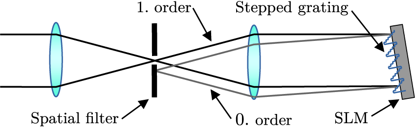
) and represents one period of the phase stepped grating (which is a discrete form of the blazed diffraction grating). The diffraction efficiency of each SP is adjustable, as shown in Figure 2, and can be as high as 71% (see Figure 9 shown later). By this approach, we spatially control the amount of incident power diffracted in the first diffraction order, and only this order passes through the spatial filter in the relay imaging telescope after the SLM.
$10\;\mathrm{px}\times 10\;\mathrm{px}$
) and represents one period of the phase stepped grating (which is a discrete form of the blazed diffraction grating). The diffraction efficiency of each SP is adjustable, as shown in Figure 2, and can be as high as 71% (see Figure 9 shown later). By this approach, we spatially control the amount of incident power diffracted in the first diffraction order, and only this order passes through the spatial filter in the relay imaging telescope after the SLM.
Principle of the beam shaping with SPs. Each triangle represents one blazed (stepped) grating and, according to the maximum phase modulation $\Phi$
, it diffracts a certain amount of energy to the first diffraction order. Diffraction to other orders is neglected for clarity.
$\Phi$
, it diffracts a certain amount of energy to the first diffraction order. Diffraction to other orders is neglected for clarity.

With this method, a fail-safe operation of the beam shaping system is guaranteed (Figure 3) as the probability that the failure creates a diffraction grating with a grating period that diffracts the beam through the spatial filter is low. In case of SLM failure, nothing is diffracted into the amplifier chain, unlike in Refs. [Reference Barczys, Bahk, Spilatro, Coppenbarger, Hill, Hinterman, Kidder, Puth, Touris and Zuegel8,Reference Bahk, Fess, Kruschwitz and Zuegel13], where the unnecessary energy is removed by diffraction and, in the case of SLM failure, some energy may still propagate into an amplifier chain. The safe operation of the beam shaping system is additionally provided by the software control discussed in Section 4.1.
Diffraction order filtering. Only the first diffraction order passes through the spatial filter after the SLM.
The diffraction efficiency of each SP is given by the intensity transmittance function (ITF), defined as follows:
 $$\begin{align}\mathrm{ITF}=\frac{\mathrm{reference}\kern0.17em \mathrm{profile}}{\mathrm{incident}\kern0.17em \mathrm{profile}},\end{align}$$
where the incident profile is the intensity distribution of the laser beam right before the SLM and the reference profile is the desired intensity distribution right after the SLM in the first diffraction order.
The reference intensity profile was selected to be the square super-Gaussian beam according to Equation (2) with $n=4$
:
$n=4$
:
 $$\begin{align}\mathrm{RF}=A\cdot \exp \left\{-\left[{\left(\frac{x-{c}_x}{h}\right)}^{2n}+{\left(\frac{y-{c}_y}{h}\right)}^{2n}\right]\right\},\end{align}$$
where RF is the reference profile, $A$
is the amplitude,
$A$
is the amplitude, $x$
,
$x$
, $y$
are the horizontal and vertical coordinates, respectively,
$y$
are the horizontal and vertical coordinates, respectively, ${c}_x$
,
${c}_x$
, ${c}_y$
are the beam center coordinates,
${c}_y$
are the beam center coordinates, $h$
controls the beam width and
$h$
controls the beam width and $n$
is the order of the super-Gaussian function.
$n$
is the order of the super-Gaussian function.
While the required pixel phase range of the SLM for the above-explained shaping is $2\pi\;\mathrm{rad}$
and the phase range of our SLM is
$2\pi\;\mathrm{rad}$
and the phase range of our SLM is $4.6\pi\;\mathrm{rad}$
, the rest can be used for the shaping of the wavefront of the incident beam. The principle is to add a constant phase shift to each SP individually, as can be seen from Figure 4. Therefore, the maximum peak-to-valley (PV) value of wavefront modulation added by the SLM is
$4.6\pi\;\mathrm{rad}$
, the rest can be used for the shaping of the wavefront of the incident beam. The principle is to add a constant phase shift to each SP individually, as can be seen from Figure 4. Therefore, the maximum peak-to-valley (PV) value of wavefront modulation added by the SLM is $1.3\lambda$
. Similarly to the ITF, the phase transmittance function (PTF) is computed from the reference wavefront and incident wavefront:
$1.3\lambda$
. Similarly to the ITF, the phase transmittance function (PTF) is computed from the reference wavefront and incident wavefront:
 $$\begin{align}\mathrm{PTF}=\mathrm{reference}\kern0.17em \mathrm{wavefront}-\mathrm{incident}\kern0.17em \mathrm{wavefront},\end{align}$$
and the obtained function gives the constant phase modulation (in $\lambda$
) for each SP that can be directly displayed on the SLM without any conversion.
$\lambda$
) for each SP that can be directly displayed on the SLM without any conversion.
Principle of the wavefront shaping with SPs. Each SP represents one blazed (stepped) grating, and according to the individual constant phase shift, each SP adds a spatially distributed phase delay. The principle is explained on the zeroth diffraction order and diffraction to other orders is neglected for clarity.

2.1 SLM and camera spatial registration
The beam shaping based on the ITF can only work with exact information of the location of the beam on the SLM. During the process of spatial calibration, spots with no intensity (holes), the Gaussian edge profile and well-defined positions are created by the SLM in the beam and captured by the near-field camera. The location of each hole in the camera image is then detected, and together with the information about the location of holes on the SLM, a spatial transformation is obtained. A similar technique was used in Refs. [Reference Barczys, Bahk, Spilatro, Coppenbarger, Hill, Hinterman, Kidder, Puth, Touris and Zuegel8,Reference Zhao, Liang, Li, Zong, Tang, Zhao, Wang, Li, Zeng, Xia, Chen, Chen, Zheng, Wei and Zhu11]. The beam captured by the camera and transformed by spatial transformation is then considered as the incident beam in the ITF calculation.
2.2 Intensity calibration
The intensity calibration indicates the diffraction efficiency response as a function of the maximum phase depth of the stepped grating, as in Figure 5. Even though the analytic expression is in the form of a ${\operatorname{sinc}}^2$
function, the measured data are fit with the following:
${\operatorname{sinc}}^2$
function, the measured data are fit with the following:
 $$\begin{align}{\eta}_{\mathrm{d}}\left({\Phi}_{\mathrm{max}}\right)=a\cdot \sin \left(b{\Phi}_{\mathrm{max}}-c\right)+a,\end{align}$$
which is easily invertible on $\left\langle 0,2\pi \right\rangle$
in order to find the maximum phase modulation for the required diffraction efficiency given by the ITF. In addition, there is no need to know the exact diffraction efficiency response due to the iterative shaping algorithm (see Section 4.1). Our SLM has a
$\left\langle 0,2\pi \right\rangle$
in order to find the maximum phase modulation for the required diffraction efficiency given by the ITF. In addition, there is no need to know the exact diffraction efficiency response due to the iterative shaping algorithm (see Section 4.1). Our SLM has a $4.6\pi\;\mathrm{rad}$
phase range and only a 0–
$4.6\pi\;\mathrm{rad}$
phase range and only a 0– $2\pi\;\mathrm{rad}$
span is used for intensity shaping. The rest of the SLM’s phase range is utilized for wavefront shaping.
$2\pi\;\mathrm{rad}$
span is used for intensity shaping. The rest of the SLM’s phase range is utilized for wavefront shaping.
Normalized diffraction efficiency response of the stepped grating as a function of the maximum phase modulation ${\Phi}_{\mathrm{max}}$
. Measured data are fit with Equation (4).
${\Phi}_{\mathrm{max}}$
. Measured data are fit with Equation (4).

3 Bivoj laser system
The Bivoj laser system (Figure 6) is a multi-slab high-energy nanosecond diode pumped solid-state laser with high average power[ Reference Mason, Divoký, Ertel, Pilař, Butcher, Hanuš, Banerjee, Phillips, Smith, De Vido, Lucianetti, Hernandez-Gomez, Edwards, Mocek and Collier 18 , Reference Banerjee, Mason, Ertel, Phillips, De Vido, Chekhlov, Divoky, Pilar, Smith, Butcher, Lintern, Tomlinson, Shaikh, Hooker, Lucianetti, Hernandez-Gomez, Mocek, Edwards and Collier 28 ]. Recently, a 150 J operation at a 10 Hz repetition rate and a 10 ns pulse length was achieved[ Reference Divoký, Pilař, Hanuš, Navrátil, Denk, Severová, Mason, Butcher, Banerjee, De Vido, Edwards, Collier, Smrž and Mocek 29 ]. The system consists of three main sections, which are the front-end (FE) with two preamplifiers (PA1, PA2) and two main power cryo-amplifiers (MA1, MA2), as Figure 6 shows. Figure 1 represents the beam intensity profile in the second preamplifier (PA2) in the FE that degraded due to the nonuniform gain. PA2 increases the pulse energy up to 50 mJ.
Laser system Bivoj model. PA, room temperature preamplifier; MA, main cryo-amplifier; D, diode pumping module; cGC, cryogenic gas cooler. Reprinted with permission from Ref. [Reference Divoky, Pilar, Hanus, Navratil, Sawicka-Chyla, De Vido, Phillips, Ertel, Butcher, Fibrich, Green, Koselja, Preclikova, Kubat, Houzvicka, Rus, Collier, Lucianetti and Mocek27], © Optica.

After the PA2, the first main cryo-amplifier (MA1) increases the pulse energy up to 14 J and tends to smooth the beam intensity profile because the cryo-cooled active ytterbium-doped yttrium aluminum garnet (Yb:YAG) slabs are working in saturation. This is observed especially at higher output pulse energies. A wide range of beam users and applications also require lower pulse energies (e.g., around $\sim$
2 J) when the beam profile is not smoothed in MA1.
$\sim$
2 J) when the beam profile is not smoothed in MA1.
The beam shaping system was implemented into the front-end of the Bivoj laser system. The front-end begins with a continuous-wave (CW) fiber oscillator. The CW beam is then shaped in the temporal domain by an acousto-optic modulator, amplified in a fiber amplifier and finally shaped in the temporal domain again by an electro-optic modulator. Pulses with arbitrary shape and pulse duration of 2–14 ns are generated with the output energy of 10 nJ for a 10 ns pulse. The pulses are then amplified by the regenerative amplifier (PA1) based on the $\mathrm{Yb}{:}{\mathrm{CaF}}_2$
rod to approximately 4 mJ with the repetition rate of 10 Hz. After PA1, the 2 mm Gaussian beam is spatially shaped to
$\mathrm{Yb}{:}{\mathrm{CaF}}_2$
rod to approximately 4 mJ with the repetition rate of 10 Hz. After PA1, the 2 mm Gaussian beam is spatially shaped to $8\;\mathrm{mm}\times 8\;\mathrm{mm}$
square with the super-Gaussian profile in the beam shaper consisting of the expanding telescope, the
$8\;\mathrm{mm}\times 8\;\mathrm{mm}$
square with the super-Gaussian profile in the beam shaper consisting of the expanding telescope, the $\pi$
-shaper and the serrated aperture with the spatial filter.
$\pi$
-shaper and the serrated aperture with the spatial filter.
After the shaping, the beam passes through the polarization beam splitter and the Faraday rotator and is relay-imaged onto the SLM by the spatial filtering telescope. Finally, a half-wave plate (HWP) is used to adjust polarization before the SLM (Figure 7). The SLM (model X13138-03 by Hamamatsu) has $1272\;\mathrm{px}\times 1024\;\mathrm{px}$
resolution, 12.5 μm pixel pitch, 96% fill factor and
$1272\;\mathrm{px}\times 1024\;\mathrm{px}$
resolution, 12.5 μm pixel pitch, 96% fill factor and $15.8\;\mathrm{mm}\times 12.8\;\mathrm{mm}$
active area size. The maximum phase modulation is around
$15.8\;\mathrm{mm}\times 12.8\;\mathrm{mm}$
active area size. The maximum phase modulation is around $4.6\pi\;\mathrm{rad}$
with a 12-bit driving signal. The SLM is adjusted in such a way that only the first diffraction order passes through the pinhole of the spatial filter on its way back to the Faraday rotator. This ensures the safety of the system in the case of SLM failure. The telescope before the SLM also modifies the beam size (
$4.6\pi\;\mathrm{rad}$
with a 12-bit driving signal. The SLM is adjusted in such a way that only the first diffraction order passes through the pinhole of the spatial filter on its way back to the Faraday rotator. This ensures the safety of the system in the case of SLM failure. The telescope before the SLM also modifies the beam size ( $\sim 11\;\mathrm{mm}\times 11\;\mathrm{mm}$
) according to the SLM active area size.
$\sim 11\;\mathrm{mm}\times 11\;\mathrm{mm}$
) according to the SLM active area size.
Scheme of the front-end beam shaping section of the Bivoj laser system.
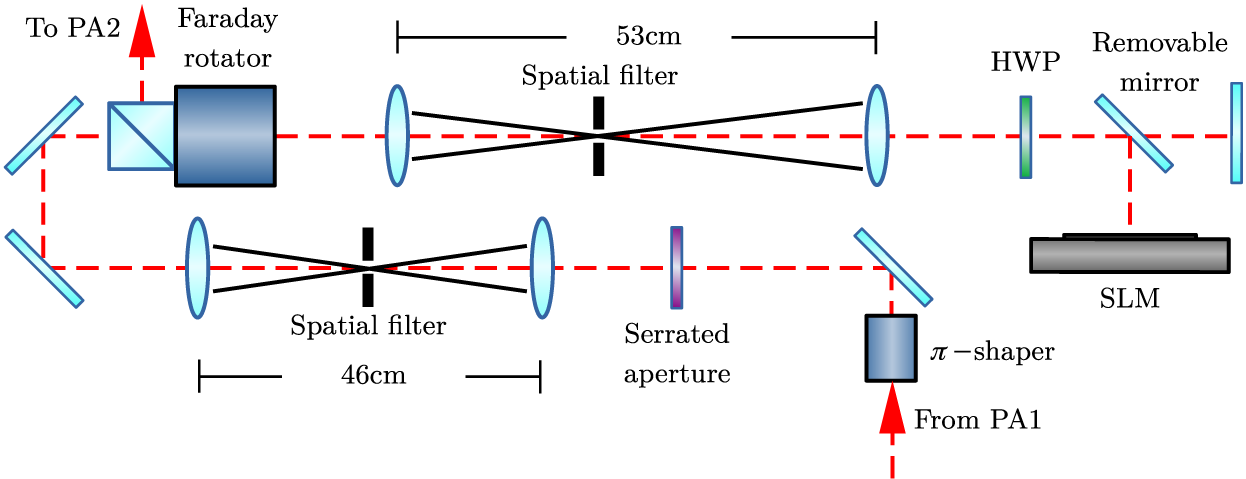
After the telescope, the beam passes through the Faraday rotator and is reflected by the polarization beam splitter to the second preamplifier (PA2), where pulses are amplified to the energy of approximately 50 mJ. PA2 is an eight-pass amplifier based on a Yb:YAG and preserves the square super-Gaussian beam profile, which is subsequently expanded to $21\;\mathrm{mm}\times 21\;\mathrm{mm}$
and injected into the 10 J main cryo-amplifier. A detailed description of the main cryo-amplifiers and the overall system can be found in Ref. [Reference Divoky, Smrz, Chyla, Sikocinski, Severova, Novak, Huynh, Nagisetty, Miura, Pilař, Slezak, Sawicka, Jambunathan, Vanda, Endo, Lucianetti, Rostohar, Mason, Phillips, Ertel, Banerjee, Hernandez-Gomez, Collier and Mocek2]. The SLM was implemented in the system using a removable mirror that, if removed, allows the system to operate without the SLM. The near-field feedback camera is located after PA2 in the SLM relay-image plane.
$21\;\mathrm{mm}\times 21\;\mathrm{mm}$
and injected into the 10 J main cryo-amplifier. A detailed description of the main cryo-amplifiers and the overall system can be found in Ref. [Reference Divoky, Smrz, Chyla, Sikocinski, Severova, Novak, Huynh, Nagisetty, Miura, Pilař, Slezak, Sawicka, Jambunathan, Vanda, Endo, Lucianetti, Rostohar, Mason, Phillips, Ertel, Banerjee, Hernandez-Gomez, Collier and Mocek2]. The SLM was implemented in the system using a removable mirror that, if removed, allows the system to operate without the SLM. The near-field feedback camera is located after PA2 in the SLM relay-image plane.
4 PA2 nonuniform gain correction
4.1 Closed-loop operation
The shaping algorithm is based on a feedback from the near-field camera that is placed after PA2. In this configuration, when the pulses are amplified in PA2, the shaping loop must also take into account the dynamic processes in the amplifier itself (such as intensity saturation) and the inaccuracy of the grating efficiency curve (Figure 5). We therefore correct the beam intensity profile deformations in an iterative way, when in each iteration only a partial correction is applied. The feedback camera, SLM and PA2 gain medium are relay-imaged one to each other.
The diagram of the shaping algorithm is shown in Figure 8. It is based on the ITF, but in each iteration only a small portion of the ITF is applied. This is represented as the ITF contrast reduction according to the following equation:
 $$\begin{align}\overline{{T}}=k\cdot \left({T}-m\right)+m,\end{align}$$
where $k$
is the coefficient of the iterative algorithm,
$k$
is the coefficient of the iterative algorithm, ${T}$
is the matrix representing the calculated ITF for each
${T}$
is the matrix representing the calculated ITF for each $\mathrm{SP}$
,
$\mathrm{SP}$
, $m$
is the average value of the
$m$
is the average value of the ${T}$
matrix and
${T}$
matrix and $\overline{{T}}$
is the ITF with reduced contrast. This ensures the correction of inaccuracies in the efficiency response curve. The coefficient of the iterative algorithm
$\overline{{T}}$
is the ITF with reduced contrast. This ensures the correction of inaccuracies in the efficiency response curve. The coefficient of the iterative algorithm $k$
influences the quality and speed of shaping and is determined by the user. After the contrast reduction, the ITF is multiplied with the one from the previous iteration and normalized to 1. The control algorithm monitors the beam after each iteration for intensity spikes before proceeding to next iteration to avoid potential damage in the laser system.
$k$
influences the quality and speed of shaping and is determined by the user. After the contrast reduction, the ITF is multiplied with the one from the previous iteration and normalized to 1. The control algorithm monitors the beam after each iteration for intensity spikes before proceeding to next iteration to avoid potential damage in the laser system.
Iterative shaping algorithm schematic. At the beginning of the iteration, the ITF is obtained from the actual and reference beam profiles. Then, the contrast of the ITF is reduced; it is multiplied with the previous ITF, normalized and sent to the SLM.

4.2 Beam quality coefficient and shaping efficiency
The quality of the beam intensity profile is described with beam quality coefficients (BQCs) – the intensity contrast and deviation from the reference profile. The first describes only the quality of the beam plateau and the second characterizes the beam intensity distribution as a whole.
Intensity contrast indicates the uniformity of the beam plateau:
 $$\begin{align}\mathrm{IC}=\frac{I_{\mathrm{max}}-{I}_{\mathrm{min}}}{I_{\mathrm{max}}+{I}_{\mathrm{min}}},\end{align}$$
where ${I}_{\mathrm{max}}$
and
${I}_{\mathrm{max}}$
and ${I}_{\mathrm{min}}$
correspond to the maximum and minimum average pixel intensity, respectively, measured over any area within the plateau region equivalent to
${I}_{\mathrm{min}}$
correspond to the maximum and minimum average pixel intensity, respectively, measured over any area within the plateau region equivalent to ${10}^{-4}$
of the plateau area.
${10}^{-4}$
of the plateau area.
Deviation from reference profile is defined as a quadratic deviation:
 $$\begin{align}\mathrm{DRP}=\sqrt{\frac{1}{N-1}\sum \limits_{i=1}^N{\left({I}_i-{\overline{I}}_i\right)}^2},\end{align}$$
where ${I}_i$
is the intensity of the ith pixel in the beam image and
${I}_i$
is the intensity of the ith pixel in the beam image and ${\overline{I}}_i$
is the intensity of the ith reference pixel in the reference beam profile.
${\overline{I}}_i$
is the intensity of the ith reference pixel in the reference beam profile.
Shaping efficiency is another important characteristic of the shaping system. Two factors impact the shaping efficiency $\eta$
according to the following:
$\eta$
according to the following:
 $$\begin{align}\eta ={\eta}_{\mathrm{s}}\cdot {\eta}_{\mathrm{d}},\end{align}$$
where ${\eta}_{\mathrm{s}}$
is the efficiency of the shaping algorithm and
${\eta}_{\mathrm{s}}$
is the efficiency of the shaping algorithm and ${\eta}_{\mathrm{d}}$
is the diffraction efficiency of the used stepped diffraction grating that depends on the grating period
${\eta}_{\mathrm{d}}$
is the diffraction efficiency of the used stepped diffraction grating that depends on the grating period $\xi$
, as Figure 9 shows. According to this plot, the grating period for the shaping experiments is chosen to either maintain the maximum diffraction efficiency
$\xi$
, as Figure 9 shows. According to this plot, the grating period for the shaping experiments is chosen to either maintain the maximum diffraction efficiency ${\eta}_{\mathrm{d}}$
or to get better shaping resolution (discussed in the next section). The efficiency of the shaping algorithm
${\eta}_{\mathrm{d}}$
or to get better shaping resolution (discussed in the next section). The efficiency of the shaping algorithm ${\eta}_{\mathrm{s}}$
is caused by the removal of unwanted energy from the beam profile.
${\eta}_{\mathrm{s}}$
is caused by the removal of unwanted energy from the beam profile.
Maximum diffraction efficiency as a function of the stepped grating period $\xi$
. The larger the number of pixels in the SP, the more the phase stepped profile converges to the blazed one, which has the maximum diffraction efficiency of 100% in the first diffraction order.
$\xi$
. The larger the number of pixels in the SP, the more the phase stepped profile converges to the blazed one, which has the maximum diffraction efficiency of 100% in the first diffraction order.

4.3 PA2 output correction results
The beam shaping loop was tested by shaping the beam before PA2 to optimize its output beam. Before each shaping run, the camera background was removed by capturing an image with no diffraction on the SLM and subtracted from every subsequently captured image.
Figure 10 shows the beam intensity profile at the output of PA2 before and after the shaping run. The coefficient of the iterative algorithm was set to $k=0.1$
. The BQCs were calculated for each iteration and are plotted in Figure 11. As can be seen from the same figure, after 11 iterations, both BQCs reached values less than one-half of their initial values. After 25 iterations, the beam closely matches the desired reference profile (Figure 10) and, in subsequent iterations, its profile and BQCs oscillate around constant values.
$k=0.1$
. The BQCs were calculated for each iteration and are plotted in Figure 11. As can be seen from the same figure, after 11 iterations, both BQCs reached values less than one-half of their initial values. After 25 iterations, the beam closely matches the desired reference profile (Figure 10) and, in subsequent iterations, its profile and BQCs oscillate around constant values.
Output of the second preamplifier PA2 during shaping and the reference beam profile.

Beam quality coefficients and shaping efficiency during the shaping of the beam at the output of PA2.

The shaping efficiency was also measured (Figure 11). The stepped diffraction grating with a 14 px SP was used. Smaller sizes of SP did not improve the shaping performance, so the SP with maximum possible diffraction efficiency ${\eta}_{\mathrm{d}}$
was chosen. Therefore, the overall efficiency
${\eta}_{\mathrm{d}}$
was chosen. Therefore, the overall efficiency $\eta$
after 25 iterations was around 39% according to the plot in Figure 9. It should be noted that the designed PA2 output energy is 100 mJ, which is considerably higher than what is actually needed, and the energy losses by shaping can be easily restored by adjusting its output power.
$\eta$
after 25 iterations was around 39% according to the plot in Figure 9. It should be noted that the designed PA2 output energy is 100 mJ, which is considerably higher than what is actually needed, and the energy losses by shaping can be easily restored by adjusting its output power.
The long-time operation was tested subsequently. At the beginning of the day, the beam was shaped by the iterative algorithm after the laser was thermally stabilized. The BQCs were tracked during the 6-hour-long laser operation. The variations of IC and DRP were only minimal (DRP stayed the same and IC increased from 0.16 to 0.17) and did not have any impact on the laser system operation and so no other run of the shaping algorithm during that day was needed. This long-time operation characteristic is strongly dependent on the beam movement on the SLM. During normal operation, the beam moves significantly only at the start of the system, when all components need to reach thermal equilibrium (this takes around 45 minutes). The time necessary for the shaping operation to perform calibration routines and converge to the desired beam profile was less than 1 minute (in the 10 Hz laser regime).
The shaped beam was then injected into the first main cryo-amplifier (MA1) and amplified first to the energy of 2 J and then to the energy of 6 J. The results are shown in Figure 12. At 2 J output energy, the smoothing of the beam plateau is more visible compared to the 6 J output, when the beam plateau is also smoothed by saturation of the amplification in MA1. However, on the other hand, the saturation of the amplification causes changes in the beam edge steepness (the closed-loop works with the feedback near-field camera at the end of the front-end, so it does not consider the effect of saturation of amplification in MA1). The pump beam is a square super-Gaussian with $n=32$
according to Equation (2) and that is one of the reasons why the DRP coefficient value of the shaped beam increased after amplification in MA1 at 6 J output energy. The alignment of the amplifier can also result in uneven amplification of the beam edges because each pass through the amplifier head is directed at a slightly different angle and might not be exactly overlapped with the previous pass.
$n=32$
according to Equation (2) and that is one of the reasons why the DRP coefficient value of the shaped beam increased after amplification in MA1 at 6 J output energy. The alignment of the amplifier can also result in uneven amplification of the beam edges because each pass through the amplifier head is directed at a slightly different angle and might not be exactly overlapped with the previous pass.
Comparison of outputs from the MA1 amplifier with and without shaping. The circular diffraction patterns in the images are caused by dust particles or defects in the diagnostic optical setup and are not present in the actual beam profile.

5 Wavefront pre-compensation
The wavefront shaping capabilities were tested on the shaped beam from Figure 10. The feedback wavefront sensor (Phasics SID4) was placed after PA2 using a beamsplitter in the same SLM relay-imaged plane as the feedback near-field camera. The initial beam intensity profile distribution was first shaped by running a few iterations of the intensity shaping algorithm, and then the PTF based on the wavefront from the wavefront sensor was applied in two iterations. The wavefront data obtained from the wavefront sensor were spatially registered according to the beam edges, but the procedure introduced in Section 2.1 can also be used with this type of wavefront sensor. The results of aberration correction can be seen in Figure 13. The initial wavefront root-mean-square (RMS) value was improved by more than 10×. The effect of wavefront shaping on the intensity distribution was negligible.
Aberration correction in the front-end of the Bivoj laser system. Wavefronts were measured with a Phasics SID4 wavefront sensor at the output of the second preamplifier PA2 before and after correction.

The beam with the corrected (flat) wavefront was then injected into the MA1 amplifier and the wavefront at its output was measured. However, it was not improved significantly (in terms of RMS and PV values); only its shape was slightly different mainly because the front-end aberration magnitude is small compared to the overall aberration magnitude of MA1.
We also tried to enhance the performance of the MA1 adaptive optics system with the SLM. The deformable mirror after the third pass in the MA1 amplifier corrects thermally induced aberrations. It has $7\times 7$
actuators, so it is not able to correct higher-frequency aberrations. The aim of this experiment was to pre-compensate these aberrations with the SLM in the front-end and improve the output wavefront of MA1.
$7\times 7$
actuators, so it is not able to correct higher-frequency aberrations. The aim of this experiment was to pre-compensate these aberrations with the SLM in the front-end and improve the output wavefront of MA1.
Firstly, the wavefront at the front-end output was corrected and the same was done with the deformable mirror in the MA1 amplifier. Then, the data from wavefront sensor at the output of MA1 was used to obtain a new PTF that was sent to the SLM with the previous PTFs. However, this approach did not improve MA1’s output wavefront significantly (compared to the solo MA1 adaptive optics system performance), mainly because the high-frequency aberrations in MA1 were not static and were changing unpredictably (they are caused primarily by the fast turbulent flow of the cooling helium).
6 Creating nonordinary beam shapes
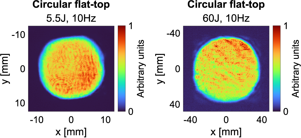
The shaping system allows one to diffract basically any beam shape that fits into the original unshaped beam. Most interesting are circular flat-top beams or annular (ring) beams, as was stated in Section 1 Motivation. These beam shapes were created with the closed-loop algorithm, injected into the Bivoj amplifier chain and amplified in both main amplifiers.
Some of the results can be seen in Figures 14 and 15. The annular beam was created by subtracting two circular super-Gaussian profiles. The square super-Gaussian profile with a circular hole was generated similarly. The hole size was chosen randomly and is around 5 mm for the ring and 4 mm for the square shape. The contrast ratio (CR) was calculated as the ratio of average intensities in the hole area to the beam plateau. The separation edge of the hole area for the CR calculation was given by the intensity threshold of 5%.
Nonordinary beam shapes at the output of the MA1 amplifier (CR, contrast ratio).

Circular flat-top beam at the output of the MA1 and MA2 amplifiers.
The maximum achievable energy for these beam shapes is given by their area ratio to the original square beam, so the fluence inside the amplifiers is preserved. The theoretical energy limit for the inscribed circular beam amplified in the MA1 and MA2 amplifiers is 78% of the full square beam.
7 Conclusions
The problem with the nonuniform gain in the second preamplifier (PA2) of the Bivoj laser system was addressed by the development of a beam shaping system based only on the single LCoS SLM and the near-field charge-coupled device (CCD) camera. The shaping system is fully automatic, a fail-safe against SLM malfunction and is incorporated directly in the main laser control system.
The beam intensity profile at the output of PA2 was successfully improved by shaping. The beam homogeneity defined by the beam quality parameters was improved two to three times and the overall shaping efficiency of 39% was reached. Consequently, the shaped beam from PA2 led to improvement of the beam profile at the output of the first main cryo-amplifier (MA1), especially at lower output energies.
The RMS of the PA2 output wavefront was improved more than 10 times by wavefront shaping. However, the wavefront pre-compensation in the front-end had no significant effect on the output wavefront of the MA1 amplifier with its adaptive optics system.
The beam shaping system allowed one to inject nonordinary beam shapes into the amplifier chain. Amplification of the circular flat-top beam in the 100 J amplifier MA2 was successful, and therefore we conclude that tailoring kW-class output beam shapes is possible and the beam shape (among other output characteristics, such as the pulse shape and length, energy and repetition rate) can be adjusted to fit the needs of individual experiments and potentially extend the application range of the Bivoj laser system.
Moreover, the shaping system can imprint a cross-reference or mask a certain part of the beam if needed.


 Open access