Introduction

To characterize the atmospheric controls on glacier mass balance and extract a climate signal from glaciers in the Southern Alps, New Zealand, a robust understanding of the surface energy balance (SEB) is needed. In the temperate maritime climate of the Southern Alps the turbulent sensible and latent heat fluxes are a key part of the SEB, contributing significantly to the energy available for ablation at the glacier surface. Point and distributed SEB studies show that turbulent heat fluxes provide ∼50% of the melt energy during the ablation season (Reference AndersonAnderson and others, 2010; Reference Gillett and CullenGillett and Cullen, 2011), while during large more infrequent melt events, turbulent heat fluxes dominate the energy balance, providing up to 80% of melt energy (Reference Marcus, Moore and OwensMarcus and others, 1985; Reference Hay and FitzharrisHay and Fitzharris, 1988a). Thus, to assess the sensitivity of glacier mass balance to changes in atmospheric temperature and moisture, a robust estimation of turbulent heat fluxes is needed in energy- and mass-balance models.

Eddy covariance systems that directly measure turbulent heat fluxes are delicate and impractical for long-term studies, so energy- and mass-balance models often rely on the bulk aerodynamic method (bulk method) to calculate turbulent heat fluxes. According to Monin-Obukhov similarity theory, turbulence and turbulent heat fluxes above a surface can be related to gradients of wind speed, temperature and humidity (Reference Monin and ObukhovMonin and Obukhov, 1954). The well-constrained conditions at a glacier surface (zero wind speed and fully saturated surface) enable the bulk method to be driven with values of temperature, humidity and wind speed at a single height.

With high-quality in situ measurements of surface climate, the largest uncertainty in calculating turbulent heat fluxes using the bulk method comes from the roughness lengths of momentum (z0v), temperature (z0t) and humidity (z0q), which quantify the production of turbulence and transfer of heat and moisture towards or away from the surface. Values of z0v derived over glacier ice surfaces vary widely from 3.0 x 10–6 to 1.2 x 10–1 m (Reference Bintanja and Van den BroekeBintanja and Van den Broeke, 1995; Reference Van den BroekeVan den Broeke, 1996). Previous estimates of z0v over glacier ice surfaces in New Zealand have relied on profile methods, giving values of 2.4 x 10–3 and 1.4 x 10–2m (Reference Hay and FitzharrisHay and Fitzharris, 1988b; Reference Ishikawa, Owens and SturmanIshikawa and others, 1992). No estimates of z0t or z0q have been made and consequently all studies in New Zealand have assumed that z0v = z0t = z0q. Owing to the large range of published values for z 0 , many studies use an ‘effective’ roughness length z0eff (where z0v = z0t = z0q) as a tuning variable to match modelled and observed ablation. Values obtained using this approach to characterize the surface energy and mass balance in the Southern Alps range from 2.5 x 10–3 to 1.2 x 10–2 m (Reference Marcus, Moore and OwensMarcus and others, 1985; Reference AndersonAnderson and others, 2010; Reference Gillett and CullenGillett and Cullen, 2011). The order-of-magnitude range in previously used values of z0eff raises questions as to whether the magnitude of turbulent heat fluxes is being appropriately represented in the SEB compared with other terms controlling melt.

Turbulent heat flux parameterizations used within the bulk method in current glacier SEB models can be distinguished based on the treatment of atmospheric stability effects. Under conditions of flat homogeneous terrain, a stable atmosphere (increasing temperature with height) will resist the vertical movement of air and production of turbulence, thus reducing turbulent heat fluxes. Correspondingly, the vertical profiles of wind speed, temperature and humidity above the surface are altered, as are the relationships between turbulent heat fluxes and mean wind speed, temperature and humidity at a given level. The simplest form of parameterization used in the bulk method ignores atmospheric stability effects and assumes turbulent heat fluxes are related to logarithmic profiles of wind speed, temperature and humidity (Reference MunroMunro, 1991; Reference OerlemansOerlemans, 2000; Reference Machguth, Paul, Hoelzle and HaeberliMachguth and others, 2006). Two methods are commonly used to account for atmospheric stability effects: the first through the bulk Richardson number (Ri b) (Reference Wagnon, Sicart, Berthier and ChazarinWagnon and others, 2003; Reference Molg, Cullen, Hardy, Kaser and KlokMolg and others, 2008; Reference AndersonAnderson and others, 2010; Reference Gillett and CullenGillett and Cullen, 2011); the second through the Monin–Obukhov stability parameter (z/L) (Reference BraithwaiteBraithwaite, 1995; Reference Gerbaux, Genthon, Etchevers, Vincent and DedieuGerbaux and others, 2005 (after Reference Brun, Martin, Simon, Gendre and ColeouBrun and others, 1989); Reference Klok, Nolan and Van den BroekeKlok and others, 2005; Reference Van den Broeke, Van As, Reijmer and Van de WalVan den Broeke and others, 2005; Reference Dadic, Corripio and BurlandoDadic and others, 2008; Reference Giesen, Van den Broeke, Oerlemans and AndreassenGiesen and others, 2008; Reference Hulth, Rolstad, Trondsen and Wedøe RødbyHulth and others, 2010).

Stability functions based on these two metrics (Rib and z/L) can have a large effect on calculated turbulent heat fluxes, especially over glacier surfaces where large positive temperature gradients often exist. Their effect becomes greatest during conditions of low wind speed (<3ms–1), with calculated turbulent heat fluxes rapidly approaching zero at critical stability thresholds at approximately 0.2 (Rib) and 1 (z/L). Unrealistic turbulent heat flux reduction can lead to underestimated melt and/or runaway cooling of surface temperatures, so many authors impose limits on stability functions during periods of low wind speed, such as: (1) removing stability functions for wind speed <1.5ms–1 (Reference Gillett and CullenGillett and Cullen, 2011); (2) setting a minimum value for wind speed (Reference Brun, Martin, Simon, Gendre and ColeouBrun and others, 1989; Reference Martin and LejeuneMartin and Lejeune, 1998); or (3) limiting the reduction in turbulent heat fluxes to 25–33% (Reference Martin and LejeuneMartin and Lejeune, 1998; Reference Giesen, Andreassen, Van den Broeke and OerlemansGiesen and others, 2009).

It is essential to take into account uncertainty in glacier SEB models if robust estimates of turbulent heat fluxes are to be made. Monte Carlo simulations provide a useful method to assess the combined effects of input-variable and roughness-length uncertainty on modelled energy fluxes incorporating realistic physical feedbacks between elements of the SEB. Beyond uncertainty in automatic weather station (AWS) measurements of surface layer wind speed, temperature and humidity, errors in the measured or simulated surface temperature can alter the magnitude of calculated turbulent heat fluxes by changing the lower boundary conditions of temperature and humidity used in the bulk method. Modelled surface and subsurface temperature depend on the excess or deficit of energy at the surface (Reference Klok and OerlemansKlok and Oerlemans, 2002; Reference Molg, Cullen, Hardy, Kaser and KlokMolg and others, 2008), so errors in other components of the energy balance, importantly the incoming radiative fluxes, can have a large impact on the calculated turbulent heat fluxes.

Given the important contribution turbulent heat fluxes make to the melt energy of temperate maritime glacier surfaces, it is imperative that uncertainties inherent in modelling these terms using the bulk method are addressed. With this in mind the current paper aims to use eddy covariance data to derive appropriate roughness lengths for momentum, temperature and humidity over a bare-ice glacier surface in New Zealand. In particular the paper focuses on the differences between the roughness length for momentum and those for the scalar fluxes of temperature and humidity. Turbulent heat fluxes observed using eddy covariance are compared with those modelled with the bulk method in Monte Carlo simulations that cover a range of turbulent heat flux and surface temperature schemes. This enables us to assess the treatment of atmospheric stability within the bulk method and its effect on modelled turbulent heat fluxes, while taking into account the effects of input-data and roughness-length uncertainty and different surface temperature parameterizations. A brief overview of the field site, data collection, Monte Carlo SEB simulations and eddy covariance data treatment is given before the results are presented and discussed.

Methods

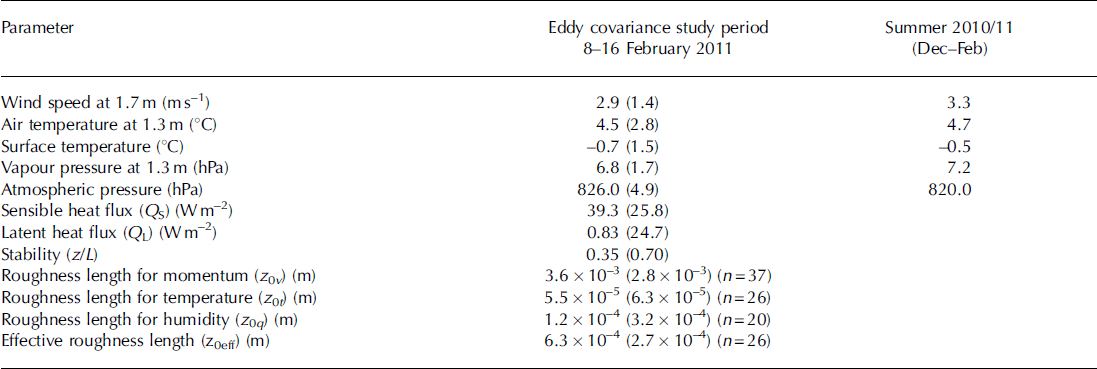
The study uses data collected from Brewster Glacier, a small mountain glacier situated in the Southern Alps of New Zealand just to the west of the main divide (Fig. 1). Brewster Glacier has a southerly aspect, a surface area of 2.5 km2 and an elevation ranging from 1660 to 2400 m a.s.l. Data are utilized from two AWS: one on the central flowline of the glacier at 1760ma.s.l. (AWSGlacier) and a second long-term station situated adjacent to the proglacial lake at 1650 m a.s.l. (AWSLake). Mean annual air temperature at AWSGlacier was 1.1 8C (October 2010-October 2011) and precipitation ∼5mw.e.a– 1 , split evenly between snow and rain. Summer (December-February) climate at AWSGlacier is characterized by moderately positive air temperatures (Table 1), an average wind speed of 3.3 m s–1 and an average vapour pressure in excess of that at the glacier surface (mean of 7.2 hPa). The lower part of the glacier (<2000m and 1.9 km2 of its total area) is gently sloping (11 8 mean slope), while the upper and smaller part of the glacier situated below the summit of Mount Brewster is steep (318 mean slope) and contains a number of large ice cliffs. The glacier surface in the vicinity of AWSGlacier has an approximate mean gradient of 68.

Fig. 1.

Map of Brewster Glacier showing locations of AWS and surrounding topography. Contours are at 100 m intervals. Long-term mass-balance network (MB stakes) shown as filled circles.

Table 1.

Means and standard deviation (in parentheses) of climate (AWSGlacier) and turbulence data during the eddy covariance measurement period and long-term data from AWSGlacier during 2010/11. Roughness lengths are log mean values. Mean turbulent heat fluxes are obtained by the eddy covariance method using only stationary runs (168)

Data from AWSGlacier were used to force a surface energy-and mass-balance model (Reference Molg, Cullen, Hardy, Kaser and KlokMolg and others, 2008) that uses Eqn (1) to describe the SEB:

where Sin is the measured incoming solar radiation (corrected for slope angle; Reference Van AsVan As, 2011), a is the temporally averaged accumulated albedo (Reference Van den Broeke, Van As, Reijmer and Van de WalVan den Broeke and others, 2004), Lin is the measured incoming longwave radiation, a is the Stefan-Boltzmann constant (5.87 x 10–8Wm–2), e is the emissivity of snow/ice (equal to unity), T0 is the surface temperature (K), QS and QL are the turbulent sensible and latent heat fluxes, respectively, QR is the rain heat flux and QC is the conductive heat flux through the glacier subsurface. Positive SEB values represent energy available for melting (QM) w hi l e the SEB is equal to zero for T0<273.15K. Energy fluxes directed towards the surface are treated as being positive. A number of different schemes to calculate T0 and QC were tested as were different parameterizations for QS and QL, with details of these provided later. QR was calculated from tipping-bucket rain gauge measurements at AWSLake.

The bulk aerodynamic equations used to calculate QS and QL within the surface energy- and mass-balance model are:

where cp is the specific heat of air at constant pressure (1005 J kg–1 K–1), p0 is the density of air at standard sea level (1.29 kg m–3 at 08C), Lv is the latent heat of vaporization (2.514MJ kg-1), replaced by the latent heat of sublimation (2.848MJ kg–1) if surface temperature (T0) is below the melting point, p is the actual air pressure (hPa), p0 is the air pressure at standard sea level (1013hPa), C is a dimensionless exchange coefficient, Uz, Tz and ez are the wind speed (ms–1), air temperature (K) and vapour pressure (hPa) at height z (m), respectively, and e0 is the vapour pressure (hPa) at the surface. Four turbulent heat flux parameterizations used in current glacier SEB models were tested within the SEB model and are defined through the treatment of atmospheric stability effects on the exchange coefficient (C). The first parameterization assumes that the turbulent heat fluxes are proportional to the neutral logarithmic profiles of wind speed and temperature with C given by:

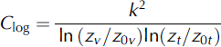
where k is the von Karman constant (0.4), zv and zt are the height of wind speed and temperature measurements, respectively, and z0v and z0t are the roughness lengths for momentum and temperature, respectively. Humidity measurements are made at zt and it is assumed that z0q =z0t . The second parameterization includes a stability function based on the bulk Richardson number (Rib) using the equation given by Reference MonteithMonteith (1957), which leads to a flux reduction in stable conditions that is less than standard formulations (e.g. Reference Wagnon, Sicart, Berthier and ChazarinWagnon and others, 2003):

The third (Cz/L) and fourth (CSR) parameterizations include an iterative stability function based on the Monin–Obukhov stability parameter z/L, where L is the Obukhov length scale (Reference Van den Broeke, Van As, Reijmer and Van de WalVan den Broeke and others, 2005):

where m and h are the vertically integrated stability functions for momentum and heat, respectively. The expressions of Reference Holtslag and de BruinHoltslag and de Bruin (1988) and Reference DyerDyer (1974) are used to define for stable and unstable conditions, respectively. The calculation of requires an estimate of QS, so Eqns (2) and (6) are calculated iteratively. In all parameterizations both z0v and z0t (=z0q) were fixed to the log mean values obtained from eddy covariance measurements except for CSR, where z0t (= z0q) is defined by surface renewal theory using the expressions of Reference AndreasAndreas (1987).

Eddy covariance measurements were made adjacent to AWSGlacier over a midsummer ice surface from 8 to 16 February 2011. Surface climate during the period was characterized by moderate wind speed and vapour pressure, with a mean air temperature of 4.5°C (Table 1). Eddy covariance instruments were mounted at 1.1 m with –0.2 m surface height change during the study period. Three-dimensional (3-D) wind speed, sonic temperature (CSAT3, CSI) and vapour density (KH20, CSI) fluctuations were recorded at 20 Hz. The instruments were levelled to horizontal at daily intervals, with minimal change noted. Before calculating turbulence statistics, coordinate rotation was applied to the velocity data to align the streamlines into the mean flow for each 30min run using a three-rotation scheme (Reference Kaimal and FinniganKaimal and Finnigan, 1994). Eddy covariance data were corrected for high-frequency flux loss due to the path-length averaging and separation of the CSAT3 and KH20 sensors (0.13 m), with average increases of 5-15% (Fig. 2a). Mean sonic temperature and sensible heat flux data were corrected for the effect of humidity fluctuations using the method of Reference Schotanus, Nieuwstadt and BruinSchotanus and others (1983). The latent heat flux data were corrected for oxygen absorption by the KH20 (Reference Tanner, Swiatek and GreeneTanner and others, 1993) and density effects using the ‘WPL’ correction (Reference Webb, Pearman and LeuningWebb and others, 1980), with corrections in the latent heat flux typically ±10% (Fig. 2b). Larger corrections only occurred when absolute fluxes were small.

Fig. 2.

Corrections to eddy covariance fluxes for (a) loss of high-frequency signal due to path-length averaging and sensor separation and (b) density and oxygen fluctuations in the path of the KH20 vapour density sensor.

The covariances of the 3-D wind velocities (u, v, w), temperature (T) and vapour density (pv) were transferred to the friction velocity (u*), temperature scale (#*) and specific humidity scale (q*) using:

where pa is the air density at the mean temperature and pressure of AWSGl a c i e r (1.046 kg m–3). These turbulent scales were then used to derive roughness lengths for each run of data using (e.g. Reference Cullen, Molg, Kaser, Steffen and HardyCullen and others, 2007):

where Uz and Tz were determined using mean values of wind speed and temperature from the eddy covariance system, and specific humidity (qz ,0) was calculated using Tz0 and relative humidity from AWSGl acier (Reference BuckBuck, 1980), assuming the surface was at saturation (6.13hPa). Vapour pressures were converted to specific humidity (kg kg-1) using qz0 = 0.622 x ez0/p.

A series of filters was applied to the 343 30min runs obtained during the study period, to remove scatter and derive reliable roughness lengths. Data during precipitation events were removed, as these greatly increase measurement errors associated with the sonic anemometer. Wind direction was restricted to a 60° sector around the glacier fall line to minimize sensor arm interference and ensure the longest on-glacier fetch. Only stationary runs were used, following the method of Reference FokenFoken (2008). Again, the stability functions of Reference Holtslag and de BruinHoltslag and de Bruin (1988) and Reference DyerDyer (1974) were used to define for stable and unstable conditions, respectively, but only runs with near-neutral conditions (-0.1 <z/L<0.1) were selected, so the choice of stability functions was not important. Runs were also selected for Uz>3.0ms–1 and u*>0.1ms–1, as errors in deriving z0v become comparatively large as these values decrease, leaving a total of 37 runs. This small sample reflects the fact that situations of near-neutral stability on mid-latitude glaciers with katabatic forcing are fairly rare, as observed by Reference Smeets, Duynkerke and VugtsSmeets and others (1998) who found only 55 half-hour periods that met the same conditions as above during the 2 month PASTEX (Pasterze experiment) campaign in Austria.

Another important consideration for deriving roughness lengths over glacier surfaces is to ensure that measurements are not affected by a low wind speed maximum. The difference in mean wind speed between the CSAT3 at 1.1 m and the RM Young anemometer at 1.7 m was used as a simple measure of wind shear in the vicinity of the eddy covariance measurements. During the conditions used to derive z0v, wind speed was found to increase above the eddy covariance measurement height, so we are confident that the roughness lengths have been derived sufficiently below any wind speed maximum. Further analysis of the wind shear over a range of stabilities is described in the next section.

To determine z0t, the gradient of temperature between the surface and the height of measurement must be well constrained. An uncertainty associated with the measured surface temperature of ±1°C (Table 2) can cause an order-of-magnitude uncertainty in the calculated value of z0t. To remove this uncertainty we selected data only when T 0 >- 1 ° C and T z > 1 °C (to ensure sufficient temperature gradient) and assumed the glacier surface was melting during these conditions (Reference CalancaCalanca, 2001). This resulted in a total of 26 runs to derive z0t. To ensure a sufficient moisture gradient to derive z0q, a minimum vapour pressure gradient of |0.66| hPa was imposed, leaving 20 runs for the calculation

Table 2.

Variables measured and sensor specifications of AWSGlacier and eddy covariance instruments

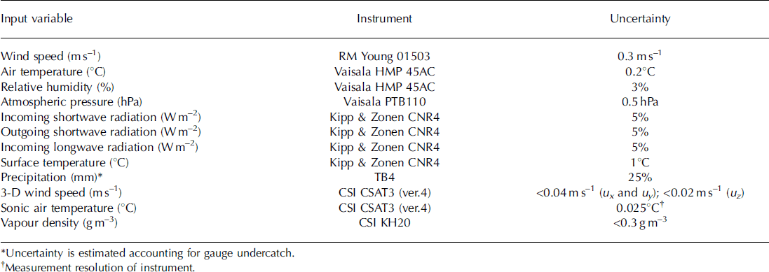
Monte Carlo simulations were made with the SEB model for the period of eddy covariance measurement (cf. Reference Machguth, Purves, Oerlemans, Hoelzle and PaulMachguth and others, 2008) to assess the effect of input variable and roughness length uncertainty on turbulent heat fluxes calculated with the bulk method. A total of 40 000 simulations was conducted, with systematic and random errors being assigned to each input variable before each simulation and time-step, respectively. Errors were calculated by multiplying the uncertainties associated with each input variable (Table 2) by normally distributed random numbers (/i = 0; <r=1). Uncertainty in the derived value for z0v was also included by calculating the roughness length at each time-step (i) using:

where NORMRND(/i, a ) is a MATLAB function that selects a random number from a normal distribution with a mean (/i) of 0 and standard deviation (a) of 0.274, which is the standard deviation of the 37 logarithmically transformed roughness length values. Four surface temperature schemes were used to calculate T0 and QC: (1) measured outgoing longwave radiation; (2) an iterative energy-balance closure scheme (Reference Molg, Cullen, Hardy, Kaser and KlokMolg and others, 2008); (3) a residual flux scheme in a surface layer of 0.2 m (Reference Klok and OerlemansKlok and Oerlemans, 2002); and (4) setting T 0 at melting point for the entire period. At the start of each SEB simulation, one of the four turbulent heat flux parameterizations was randomly assigned in combination with one of the four surface temperature schemes. The modelled turbulent heat fluxes were then collated into the 16 resulting combinations before calculating means and standard deviations of QS and QL for each combination (n ∼2500) at each time-step. The resulting mean modelled turbulent heat fluxes were then compared with those observed with the eddy covariance instruments.

Results and Discussion

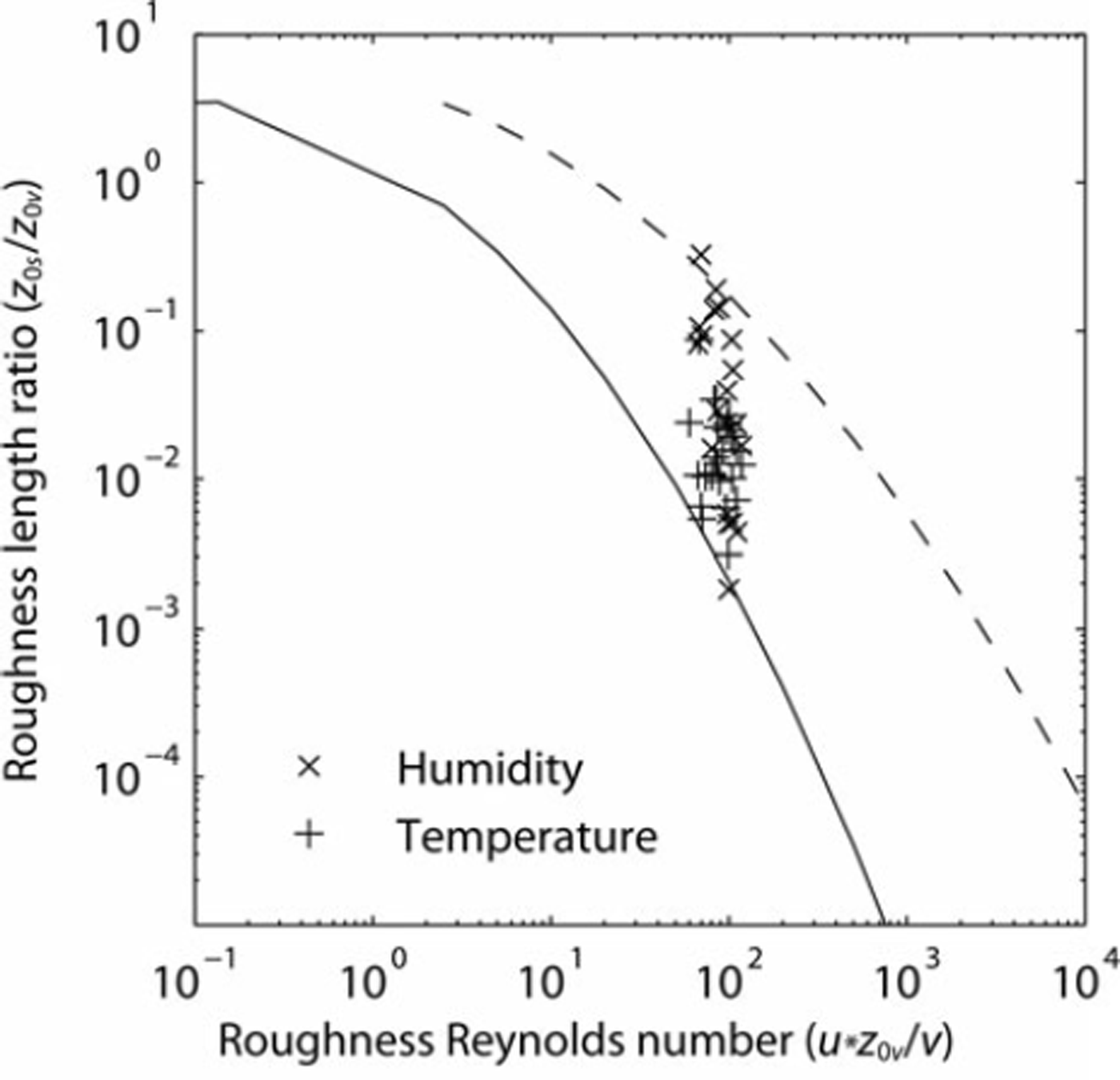
The roughness length for momentum (z0v) derived from eddy covariance was found to have a log mean value of 3.6 x 10–3 m (Table 1). This is similar to other values derived over mid-latitude glacier ice surfaces in the Southern Alps (Reference Ishikawa, Owens and SturmanIshikawa and others, 1992) and the European Alps (Reference Van den BroekeVan den Broeke, 1997; Reference Greuell and SmeetsGreuell and Smeets, 2001). More importantly, the roughness length for temperature (z0t) shows a log mean value of 5.5 x 10–5 m (Table 1), giving a ratio between the two roughness lengths (z0/z0v) of 0.015. That z0t is several orders of magnitude smaller than z0v compares well with surface renewal theory, with large roughness Reynolds numbers (Re= u*z0v/v) indicating a rough flow regime. The measured ratios lie between the predictions of Reference AndreasAndreas (1987) and those of Reference Smeets and Van den BroekeSmeets and Van den Broeke (2008), derived for hummocky ice with z0v >1 x 10–3 m (Fig. 3). The roughness length for humidity (z0q) was found to have a log mean value of 1.2 x 10–4m (Table 1). This is slightly larger than z0t, though the two values lie within one standard deviation of each other and the values are certainly within the measurement uncertainty associated with the determination of z0q. Thus, our results do not support the idea that the roughness lengths for momentum and scalar fluxes can be assumed equal, and find that z0t and z0q are approximately two orders of magnitude smaller than z0v in an aerodynamically rough flow, as found over other mid-latitude glacier surfaces (Reference Smeets, Duynkerke and VugtsSmeets and others, 1998). Our data do, however, support the use of equal roughness lengths for temperature and humidity.

Fig. 3.

The ratio of the roughness lengths for scalars (z0t and z0q) and momentum (z0v) versus roughness Reynolds number (Re). Also shown are the theoretical predictions of Reference AndreasAndreas (1987) (solid line) and Reference Smeets and Van den BroekeSmeets and Van den Broeke (2008) (dashed line). Points are individual 30min runs and the log mean value of z0v is used to calculate Re.

To allow a comparison with ‘effective’ roughness lengths used previously in glacier SEB modelling, we derive a single ‘effective’ roughness length (z0eff) that assumes equality of the momentum and scalar roughness lengths, based on the same sample used to derive z0t. The resulting log mean z0eff is 6.3 x10–4m (Table 1), almost an order of magnitude smaller than those previously used in mass-balance modelling in the Southern Alps (Reference Marcus, Moore and OwensMarcus and others, 1985; Reference Hay and FitzharrisHay and Fitzharris, 1988b). As z0t is several orders of magnitude smaller than z0v in an aerodynamically rough flow, the values of z0eff are also at least an order of magnitude smaller than those for z0v. Consequently, for scenarios in which only z0v is derived over a glacier surface and the roughness lengths are assumed to be equal, the turbulent heat fluxes are likely to be overestimated. The potential to overestimate turbulent heat fluxes is large over temperate glaciers where a melting glacier surface presents no upper limit on z0eff unless an independent check of modelled and observed surface temperature is made outside of melting conditions.

As roughness lengths can only be derived confidently in near-neutral conditions, we gain no information on the behaviour of the sensible heat flux in moderate or strongly stable conditions that dominate over the glacier surface. A first-order check can be made by examining the observed exchange coefficient (Cobs) in more stable conditions. We derive Cobs using sensible heat flux (QS-eddy), Uz and Tz from the eddy covariance instruments using Eqn (14), filtering the runs for precipitation, fetch and stationarity, as well as Uz > 1 and Tz – T0 > 1 (90 runs):

Figure 4 shows Cobs (black circles) against the observed wind speed (Fig. 4a) and temperature difference (Fig. 4b) for each 30min run. Also shown is the expected value of Cz/L calculated using the bulk Eqns (2) and (6) across the same range of wind speed and temperature experienced during the study period (shown as dotted lines). As expected, more scatter in Cobs is found during low wind speeds and for smaller temperature differences, as measurement uncertainties become more important. A lower bound of points seems to follow the values predicted by Monin-Obukhov theory, perhaps indicating cases where a relatively high wind speed maximum allows Monin-Obukhov theory to hold. However, there is no overall trend toward decreasing Cobs for either a reduction in wind speed or an increase in temperature difference. Large values of Cobs occur during light and moderate wind speeds (1-4 ms–1) and a range of temperature differences. This implies that the magnitude of the sensible heat flux does not strictly follow Monin-Obukhov theory beyond near-neutral conditions.

Fig. 4.

Exchange coefficient (Cobs) derived from eddy covariance measurements of the sensible heat flux against (a) wind speed and (b) temperature difference between air and surface. Shown as dashed lines are the exchange coefficients expected using the Cz/L parameterization (Eqn (6)).

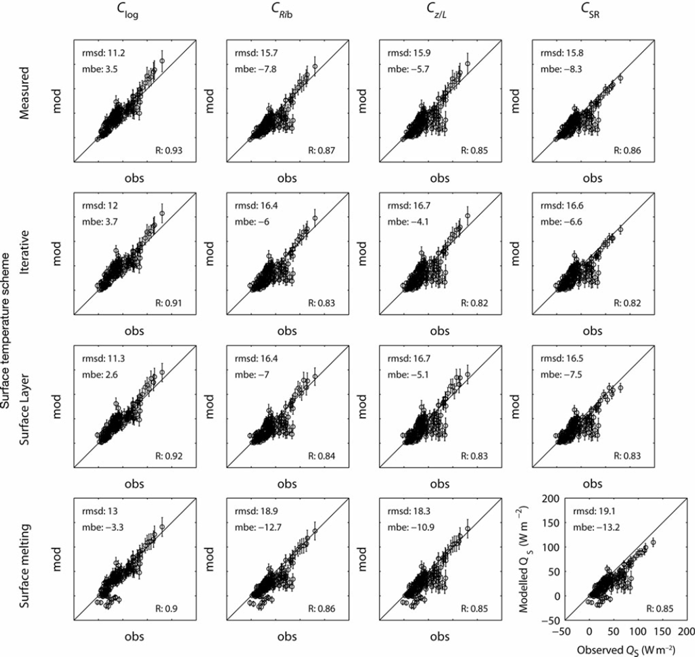
We now compare turbulent heat fluxes measured using eddy covariance (observed) with those calculated using the bulk method within the SEB (modelled). Figure 5 presents the mean sensible heat flux (QS) for each 30 min model time-step across the Monte Carlo simulations (n∼2500) for combinations of four turbulent exchange coefficient (C) parameterizations and four surface temperature schemes. Error bars show ± 1 standard deviation, and only time-steps with no precipitation and stationary eddy covariance data are shown (168 runs). The bulk method did not consistently replicate observed QS, with the performance of each parameterization within the bulk method associated with the treatment of atmospheric stability (Fig. 5). The C log parameterization produced the best fit to observed QS across the full range of temperature and wind speed, with the lowest root-mean-square difference (rmsd 11.2Wm–2 ). Some of the larger-magnitude fluxes were slightly overestimated but remain mostly within the uncertainty introduced from the input data. The small bias (2.6-3.7 Wm– 2 ) is encouraging as the use of the much simpler parameterization does not cause a large overestimate in the magnitude of QS as a whole. Parameterizations with stability functions (CRib, Cz/L, CSR) underestimate QS, independent of the surface temperature scheme used, showing biases of -4.1 to -8.3 Wm–2 . The largest underestimates occurred during periods of light wind speed (<3ms–1) and large positive gradients in temperature (>2 Km- 1 ) . During these conditions stability functions within the parameterizations dampened modelled QS close to zero while fluxes of 50-100Wm–2 were observed. A larger standard deviation in modelled QS is shown for these conditions, as uncertainties in input data become more important, but this uncertainty does not explain the underestimation.

Fig. 5.

Comparison of QS observed (CSAT3 eddy covariance system) and modelled (bulk method) for 16 combinations of sensible heat flux parameterization and surface temperature scheme. Dots and error bars show the mean and standard deviation of Monte Carlo ensembles with ∼2500 simulations per point. The bottom right axes gives the common scale in Wm– 2 . Root-mean-square difference (rmsd; Wm– 2 ) , mean bias error (mbe; Wm– 2 ) and correlation coefficient (r) are provided inside the axes for each combination.

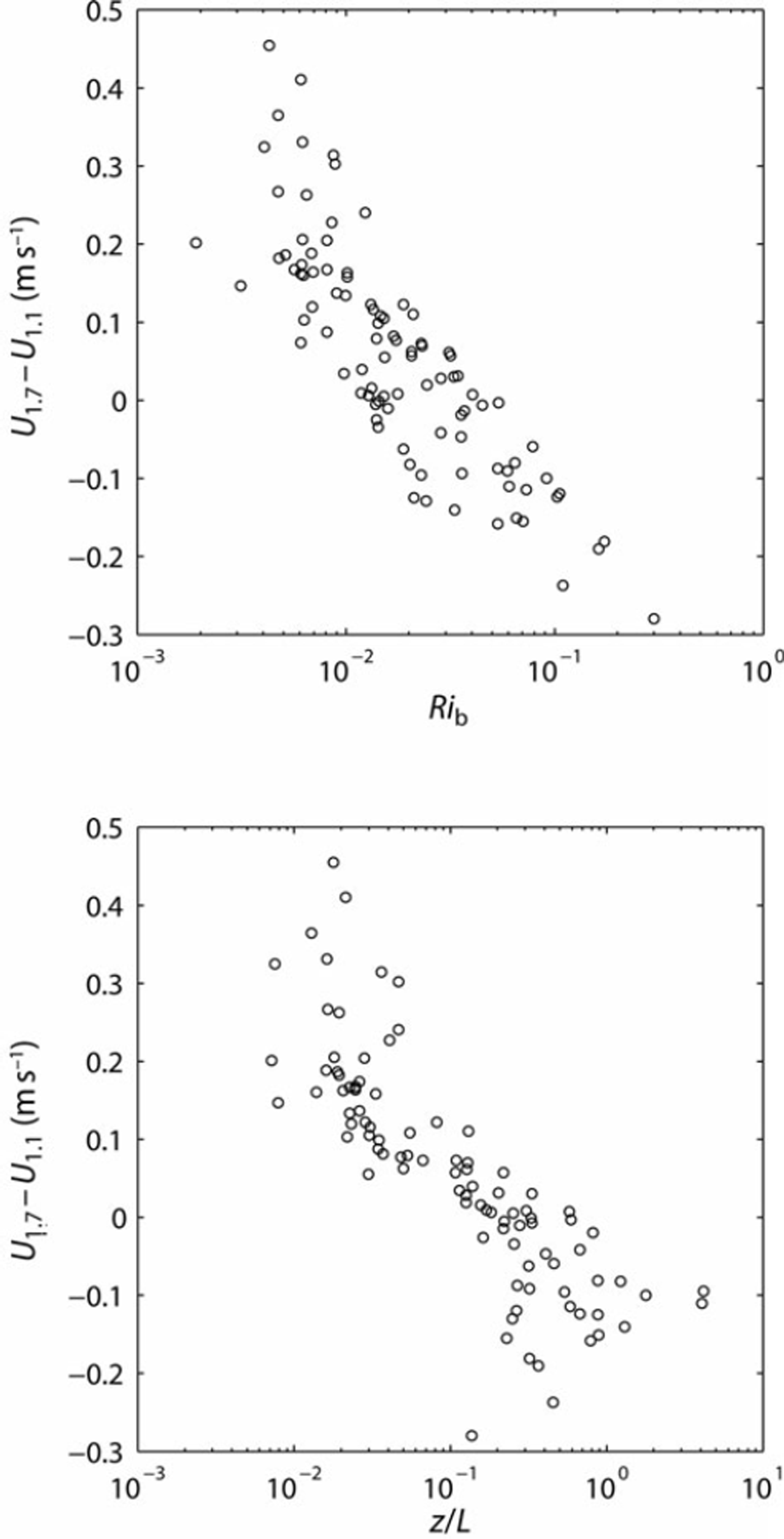
The underestimation of QS during stable conditions is likely associated with the katabatic forcing of the glacier surface layer. Over sloping glacier surfaces, a positive temperature gradient creates negative buoyancy that drives the production of turbulence, rather than inhibiting turbulence as predicted by Monin–Obukhov theory (Reference Klok and OerlemansOerlemans and Grisgono, 2002). In the katabatic flow, a wind speed maximum is formed, the height of which is proportional to the maximum wind speed of the flow and inversely related to surface slope (Reference Denby and GreuellDenby and Greuell, 2000). Under conditions of low wind speed and over a steeply sloping surface, where the height of the wind speed maximum is typically lower, even a relatively low level of measurement (<2 m) is likely to be in the region of the wind speed maximum. Figure 6 shows that for increasing atmospheric stability, as expressed through Ri b and z/L, wind shear above the eddy covariance instruments is reduced with respect to near-neutral conditions. This indicates the presence of a wind speed maximum in the vicinity of the measurements for z/L> 0.1. In the region of the wind speed maximum, turbulent transport dominates the turbulent kinetic energy budget over vertical wind shear, and the momentum flux-profile relationship returns towards that of a neutral atmosphere (Reference Denby and SmeetsDenby and Smeets, 2000). Thus, QS calculated from our level of measurement (∼1.7 m) is related to logarithmic profiles of wind speed and temperature in the presence of a wind speed maximum. Our data support this, showing that observed QS during conditions characterized by low wind speeds were best estimated using an exchange coefficient related to logarithmic wind speed and temperature profiles (Clog). A wind speed cut-off on the stability functions within CRib, Cz/L and CSR only substantially improves the estimation of QS if the stability functions are removed for wind speeds <3 m s–1 (not shown), indicating that this may be the threshold at which the effect of the wind speed maximum becomes important at this site. This is near the threshold that stability functions also start to have a large effect on QS calculated using CRib, Cz/L and CSR within the bulk method.

Fig. 6.

Wind shear between CSAT3 measurement height (1.1m) and RM Young measurement height (1.7m) versus (a) Rib and (b) z/L.

The choice of turbulent heat flux parameterization becomes critically important when assessing the sensitivity of glacier mass balance to increasing ambient air temperatures, especially in a temperate maritime environment where the turbulent heat fluxes contribute a significant fraction of the melt energy at daily and seasonal timescales. For the Clog parameterization, the modelled sensitivity of QS depends only on the change in temperature gradient between the atmosphere and glacier surface. The use of parameterizations that include stability functions (CRib, Cz/L and CSR) decreases the modelled sensitivity of melt energy to increased air temperature, as the stability functions decrease the exchange coefficient (C) and counteract an increase in temperature gradient in the calculation of QS (Eqn (2)) (cf. Reference BraithwaiteBraithwaite, 1995). In light wind conditions this can result in calculated QS decreasing as temperature increases. However, for glacier surfaces purely influenced by katabatic winds, QS is expected to increase quadratically with rising ambient temperature, as a result of a larger negative buoyancy force that amplifies the katabatic wind speed (Reference Klok and OerlemansOerlemans and Grisgono, 2002). As the katabatic turbulent heat flux model is based on the temperature deficit between the glacier surface and ambient air, it requires observations of air temperature located away from the glacier surface and is not appropriate for use with in situ observations. The Clog parameterization, in contrast to parameterizations including stability functions, will always result in increased QS as air temperature increases, thus reproducing correctly the direction of feedback predicted by the katabatic model. This is especially important over glacier surfaces where large positive temperature gradients produce significant QS even during low wind-speed conditions. The Clog parameterization will also produce a more realistic assessment of QS when gradient winds rather than katabatic flows govern the profiles of wind speed above the glacier surface. Thus, for small mountain glaciers where in situ wind-speed and temperature data are available, the use of the Clog parameterization within the bulk method is recommended. An evaluation of the temperature sensitivity over longer timescales and across the full elevation range of the glacier would be needed to further explore the impact of this sensitivity on mass balance.

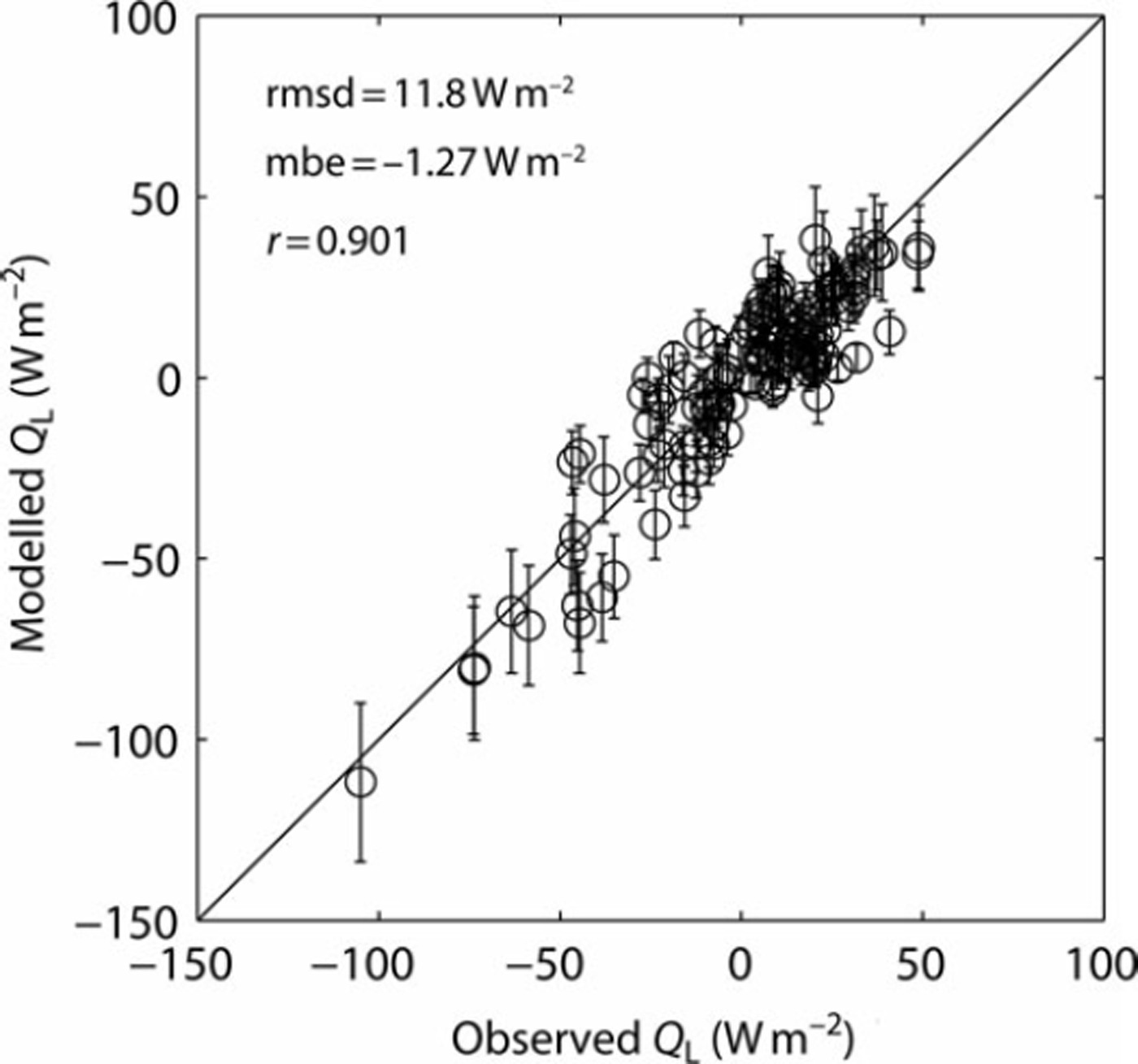
Modelled latent heat fluxes were unaffected by the choice of exchange coefficient parameterization, with very similar performance across the four parameterizations (not shown). Owing to the small vapour pressure gradient between surface and atmosphere during periods of high atmospheric stability within the study period, vapour fluxes are small during these periods and the effect of the stability correction term is not evident. To demonstrate this we show an example of modelled and observed latent heat fluxes for one set of exchange coefficient and surface temperature parameterizations (Fig. 7). The good agreement in both the magnitude and sign of observed QL (rmsd 11.8Wm–2) gives us confidence that QL can be reproduced using the bulk method using a roughness length for humidity equal to that for temperature.

Fig. 7.

Comparison of QL observed (CSAT3 eddy covariance system) and modelled (bulk method) during the ice period for the Clog parameterization. Surface temperature is calculated using the procedure described in Reference Molg, Cullen, Hardy, Kaser and KlokMolg and others (2008). Dots and error bars show the mean and standard deviation of Monte Carlo ensembles with 2618 simulations per point.

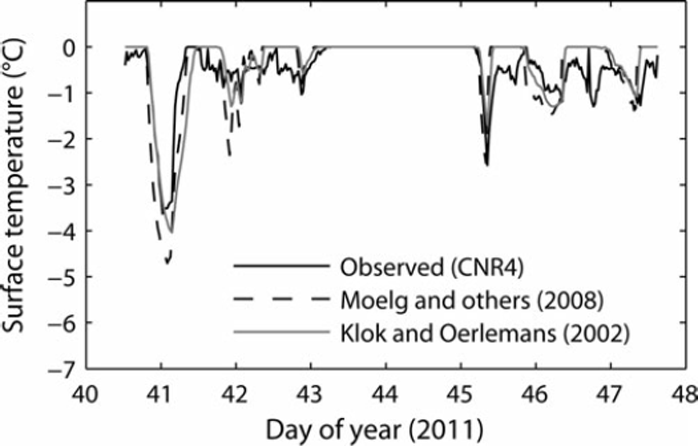
The inclusion of a realistic surface temperature scheme was important in replicating observed QS and QL. Using the assumption of a melting surface, a negative bias in QS (–3.3 to 13.2 W m–2) was produced, especially in those parameterizations using stability functions, and temporal changes in the sign of both QS and QL were not simulated correctly during periods of low (freezing) air temperatures (Figs 5 and 7). Surface temperature schemes that allowed for T0 < 08C correctly simulated QS being directed towards the surface during periods of low (freezing) air temperature (Figs 5 and 8). Since both the iterative and residual layer surface temperature schemes replicated the temporal pattern of T0 well during each study period (Fig. 8), we gain further confidence that our model incorporates the main features of the glacier SEB in a physically realistic way. The inclusion of a realistic surface temperature scheme becomes especially important when investigating the magnitude of the turbulent heat fluxes and evolution of the SEB on daily timescales. The effect of disregarding conditions of non-melting T0 on the mass balance of continental glaciers has been shown by Reference Pellicciotti, Carenzo, Helbing, Rimkus and BurlandoPellicciotti and others (2009). However, further work is needed to constrain the surface and subsurface schemes used to model temperate maritime glacier mass balance to establish the effect of non-melting conditions in this environment. Importantly, the effect of refreezing meltwater and penetrating shortwave radiation on subsurface temperatures and mass balance needs further attention.

Fig. 8.

Surface temperature during the study period showing measured surface temperature (black line) and that modelled using the expressions of Reference Molg, Cullen, Hardy, Kaser and KlokMolg and others (2008) (dashed line) and Reference Klok and OerlemansKlok and Oerlemans (2002) (grey line).

Conclusions

We have addressed a number of uncertainties in calculating turbulent heat fluxes (QS and QL) with the bulk method over a temperate maritime glacier. Eddy covariance measurements in near-neutral conditions showed a roughness length for momentum of 3.6x10–3m over the glacier ice surface. Importantly, the scalar roughness lengths of temperature and humidity were found to be approximately two orders of magnitude smaller, in agreement with surface renewal theory. Vapour flux measurements supported the common assumption that the roughness lengths for temperature and humidity are equivalent. However, using the assumption that the scalar roughness lengths are equivalent to that for momentum in an aerodynamically rough flow will lead to overestimated turbulent heat fluxes when using the bulk method. With high-quality in situ measurements of wind speed, air temperature and relative humidity, observed turbulent sensible and latent heat fluxes can be reproduced with confidence using the bulk method, but only when an exchange coefficient based on logarithmic profiles of wind speed and temperature is used. Stability functions that reduce the exchange coefficient during positive temperature gradients are shown to underestimate the sensible heat flux under low wind-speed conditions, with Monte Carlo simulations showing that input-data and roughness-length uncertainty cannot account for this. This underestimation is likely due to the influence of a katabatically driven wind-speed maximum that, over moderately sloping glacier surfaces, exists near the level of AWS measurements and alters the turbulent exchange coefficient towards that typically observed in a neutral atmosphere. The choice of exchange coefficient has important implications when assessing the effect of rising ambient air temperatures on mountain glacier mass balance, as the temperature sensitivity of the turbulent heat fluxes is increased in environments that experience katabatic flows. In order to understand the mass-balance sensitivity in detail across the full range of elevations, further work is needed to constrain other components in the SEB. In particular, parameterizations to derive incoming longwave radiative fluxes from measurements of air temperature and humidity need to be evaluated further, as do the effects of non-melting conditions, refreezing meltwater and subsurface shortwave penetration on glacier mass balance.