2. Radiatively driven convection in the linearised regime

We consider a fluid with a linear equation of state for the density $\rho =\rho _0(1-\alpha T)$, where $T$ is the temperature. We assume a negative thermal expansion coefficient $\alpha$. The fluid is subject to a radiative forcing applied to the surface. The applied heat flux $S_0{\rm e}^{z/Z_0}F(t)$ decays exponentially away from the surface and can be modulated in time (figure 1). The problem under the Boussinesq approximation can be formulated as follows:

(2.1)$$\begin{gather} \frac{{\rm D}\tilde{\boldsymbol{u}}}{{\rm D}t} ={-}\frac{1}{\rho_0}\boldsymbol{\nabla}\tilde{p} +\tilde{b} \boldsymbol{e}_3 +\nu\nabla^2\tilde{\boldsymbol{u}}, \quad \boldsymbol{\nabla}\boldsymbol{\cdot}\tilde{\boldsymbol{u}}=0, \end{gather}$$

(2.2)$$\begin{gather}\frac{{\rm D}\tilde{b}}{{\rm D}t} ={-}\frac{B}{Z_0}F(t) {\rm e}^{z/Z_0} + \kappa \nabla^2 \tilde{b}. \end{gather}$$

Here $\tilde {\boldsymbol {u}}=(\tilde {u},\tilde {v},\tilde {w})$ is the velocity, $\tilde {p}$ is the pressure deviation from the hydrostatic profile, $\tilde {b}=g(\rho _0-\rho )/\rho _0=\alpha gT$ is the buoyancy, $B=(-\alpha g S_o/\rho _0 C_p)$ is the buoyancy flux due to the radiative heat flux $S_0$, $\rho _0$ is the reference density, $C_p$ is the heat capacity, $g$ is the gravitational acceleration, $Z_0$ is the $e$-folding decay scale of the radiation flux, $\nu$ is the molecular viscosity, $\kappa$ is the molecular heat diffusivity and $\boldsymbol {e}_3$ is the unit vector pointing upward. The surface through which radiation is applied is at $z=0$ and the domain extends below to $z=-H$. All thermodynamic quantities are evaluated at the reference temperature. Mutatis mutandis, the same configuration applies to radiation applied to the bottom of a fluid with a positive expansion coefficient, with the understanding that in this case $Z_0<0$.

Figure 1.

Schematic of RDC.

For time-independent radiation

(2.3)\begin{equation} F(t)=1, \end{equation}

while for diurnal solar radiation

(2.4)\begin{equation} F(t)=\sin(\varOmega t) \quad \text{if} \ t<\tau_{DTL}, \quad \text{else} \ 0, \end{equation}

where $\varOmega ={\rm \pi} /\tau _{DTL}$ and $\tau _{DTL}$ is the daytime length.

We decompose the motion into a basic state and perturbations:

(2.5a–c)\begin{equation} \tilde{\boldsymbol{u}}=0+\boldsymbol{u}(\boldsymbol{x},t), \quad \tilde{b}=\bar{b}(z,t)+b(\boldsymbol{x},t), \quad \tilde{p}=\bar{p}+p(\boldsymbol{x},t). \end{equation}

Here $\boldsymbol {x}=(x,y,z)$ and $\bar {b}(z,t=0)=0$. The basic state satisfies

(2.6)$$\begin{gather} 0 ={-}\frac{1}{\rho_0}\boldsymbol{\nabla}\bar{p} +\bar{b}\boldsymbol{e}_3, \end{gather}$$

(2.7)$$\begin{gather}\frac{\partial\bar{b}}{\partial t} ={-}\frac{B}{Z_0} F(t) {\rm e}^{z/Z_0}+\kappa \frac{\partial ^2 \bar{b}}{\partial z^2}. \end{gather}$$

From here, we follow the same approach used to study the stability of Rayleigh–Bénard convection (Chandrasekhar Reference Chandrasekhar1961). Subtracting the basic state momentum equation (2.6) from (2.1) and then neglecting squares of perturbations, the linearised perturbation momentum equation reads

(2.8)\begin{equation} \frac{\partial \boldsymbol{u}}{ \partial t} ={-}\frac{1}{\rho_0}\boldsymbol{\nabla} p +b\boldsymbol{e}_3 +\nu\nabla^2\boldsymbol{u}. \end{equation}

From (2.8) and the incompressibility condition we derive a single equation for the Laplacian of the vertical velocity:

(2.9)\begin{equation} \frac{\partial \nabla^2 w}{\partial t} = \nabla^2_h b + \nu \nabla^2 \nabla^2 w. \end{equation}

Here, $\nabla ^2_h=\partial ^2/\partial x^2+\partial ^2/\partial y^2$ is the horizontal Laplacian operator. Subtracting the basic state buoyancy equation (2.7) from (2.2) and then neglecting squares of perturbations, the linearised perturbation buoyancy equation reads

(2.10)\begin{equation} \frac{\partial b}{\partial t}+w\frac{\partial \bar{b}(z,t)}{\partial z} = \kappa \nabla^2 b. \end{equation}

Substituting $\nabla ^2_h b$ in (2.9) into $\nabla ^2_h$[(2.10)], these two equations can be combined as

(2.11)\begin{equation} \frac{\partial^2 \nabla^2 w}{\partial t^2} +(\nabla^2_h w) \frac{\partial \bar{b}}{\partial z} -(\nu+\kappa) \frac{\partial }{\partial t} \nabla^2 \nabla^2 w+ \nu \kappa \nabla^2 \nabla^2 \nabla^2 w=0. \end{equation}

Equations (2.7), (2.9) and (2.10) will be used to find scalings for the linear system. Equation (2.11) will be used to find the growth rate and the spatial structure of the perturbations.

3. Evolution of the background profile

With an appropriate choice of a vertical velocity scale $W_0$, a buoyancy scale $b_0$ and a time scale $t_0$ (defined in the next section), we define dimensionless vertical velocity, buoyancy, time and coordinates:

(3.1a–f)\begin{equation} \hat{w}=w/W_0, \quad \hat{b}=b/b_0, \quad \hat{t}=t/t_0, \quad \hat{x}=x/Z_0, \quad \hat{y}=y/Z_0, \quad \hat{z}=z/Z_0. \end{equation}

We also define a Reynolds number $Re\equiv W_0Z_0/\nu$ and a Péclet number $Pe\equiv W_0Z_0/\kappa$. From the buoyancy scale, we can derive a temperature scale $T_0=b_0/(-\alpha g)$. In the following we dispense from decorating non-dimensional variables, and all variables except those in § 4 are non-dimensional. The background buoyancy profile satisfies

(3.2)\begin{equation} \frac{\partial\bar{b}}{\partial t} ={-}F(t) {\rm e}^z+\frac{1}{Pe}\frac{\partial ^2 \bar{b}}{\partial z^2}, \end{equation}

where the Péclet number $Pe$ is the ratio of the perturbation time scale (defined more precisely later) to the diffusive time scale $Z_0^2/\kappa$. This equation needs to be solved subject to boundary and initial conditions. For the latter, we simply choose $\bar {b}(z,0)=0$. At the bottom $(z=-H)$ of the water column, the natural choice is a no-flux condition. At the surface, we assume that the latent, sensible and long-wavelength radiative heat flux are small compared with the incoming short-wave heat flux, and thus we approximate the surface boundary condition with a no-flux condition as well. This approximation is suggested by the observations of Austin et al. (Reference Austin, Hill, Fredrickson, Weber and Weiss2022) who report that the total increase in the heat content of the water column as a function of time can be, to a great degree of accuracy, predicted by integrating the equation for heat over the water column with no-flux conditions at both boundaries. As we shall see, for large values of $Pe$, the evolution of the perturbations is primarily controlled by the evolution of the stratification in the bulk of the water column driven by the absorbed radiation. With these boundary conditions, (3.2) can be solved by writing the solution as a standard trigonometric series. The vertical gradient of the general solution is thus

(3.3)\begin{equation} \frac{\partial \bar{b}}{\partial z}(z,t)=\sum_{m=1}^\infty a_m R(\lambda_m^2/Pe,t)\sin(\lambda_mz), \end{equation}

where the wavenumber $\lambda _m=m{\rm \pi} /H$, and the coefficients

(3.4)\begin{equation} a_m=\frac{2\lambda_m}{H}\frac{1-({-}1)^m{\rm e}^{{-}H}}{1+\lambda^2_m}. \end{equation}

The function $R(s,t)$ describes the relaxation of the solution to the stationary state (which is not steady for diurnal radiation):

(3.5)\begin{align} R(s,t)=\left\{\begin{array}{ll} \dfrac{1-{\rm e}^{-\alpha t}}{s} & \mathrm{if}\ F(t)=1\mathrm{(steady\ radiation)},\\ \dfrac{1}{s^2+\varOmega^2}\left(s\sin(\varOmega t)-\varOmega(\cos(\varOmega t)-{\rm e}^{{-}s t})\right) & \mathrm{if}\ F(t)=\sin(\varOmega t)\\ & \quad \mathrm{(diurnal \ radiation)}. \end{array}\right. \end{align}

In the case of steady radiation, $R(s, t)=R(s t,1)t$. For diurnal radiation this is not in general true. However, here we are interested in perturbations that grow on a time scale much shorter than the diurnal period, i.e. $\varOmega t\ll 1$. In this case we can approximate

(3.6)\begin{equation} R(s, t)\simeq \varOmega\frac{s t-(1-{\rm e}^{{-}s t})}{s^2}+O((\varOmega t)^2), \end{equation}

and therefore $R(s,t)\simeq R(s t,1)t^2 +O((\varOmega t)^2)$. Thus we can write a general form for the background stratification:

(3.7)\begin{equation} \frac{\partial \bar{b}}{\partial z}(z,t)=\left[\sum_{p=1}^\infty a_p R(\lambda_p^2\tau,1)\sin(\lambda_pz)\right]t^n\equiv S_n(z,\tau)t^n, \end{equation}

with $\tau = t/Pe$, $n=1,2$ for steady and unsteady radiation, respectively, and $S_n(z,\tau )$ is the term in square brackets in (3.7) with the appropriate choice for $R$, the relaxation function. Thus, for large values of the Péclet number, there are two time scales that control the evolution of the background stratification profile: the ‘fast’ time $t$ over which the profile evolves in a self-similar manner, and the ‘slow’ time $\tau$ over which the overall shape of the profile changes as the diffusive boundary layer grows at the surface. In particular, the inviscid solution

(3.8)\begin{equation} \bar{b}(z,t)={-}{\rm e}^{z}\int_0^tF(t')\,{\rm d}t' \end{equation}

is recovered in the limit $\tau \to 0$.

For finite, but small, values of $\tau$ the inviscid solution approximates well the actual solution except for the surface boundary layer whose thickness grows as $\sqrt {\tau }$ (figure 2). Of course, for this to work, the penetration depth (which in our units is 1) must be much larger than the thickness of the surface boundary layer during the time over which the analysis is carried out. In practise, this limits the analysis to times shorter than $Z_0^2/\kappa$. Thus, our analysis cannot be applied to Rayleigh–Bénard convection driven by a time-dependent surface heat flux (SHF convection), because that would require taking the $Z_0\to 0$ limit. Physically, in time-dependent SHF convection the driving signal is carried into the fluid by the developing boundary layer itself. Whereas in RDC we have a non-trivial inviscid solution which is modified over a slow time by diffusion effects, in SHF convection the inviscid solution is trivial, and the background system evolves under the slow time alone.

Figure 2.

Profiles of $\partial \bar {b}/\partial z$ normalised with fast time (solid lines) and ${\rm e}^z$ (dashed lines) for different values of $\tau$ plotted against $z/\sqrt {\tau }$. The viscous profiles depart from the inviscid solution starting at a depth which deepens as $\sqrt {\tau }$.

4. Scaling and normalisation

In this section, we temporarily revert to dimensional quantities. There are two length scales in RDC: the depth of water $H$ and the radiation penetration scale $Z_0$. As near-surface water warms gradually and just starts to sink, the depth of water during the initial stages of RDC should not play a role provided $H/Z_0\gg 1$. Thus $Z_0$ is the natural length scale during the onset of this process.

The basic state is the time-dependent solution to (2.7) given by (3.7). Clearly, both $\bar {b}$ and $\partial \bar {b}/\partial z$ change continuously over time. Thus, perturbations grow against a background state which is itself changing.

We derive scales by balancing the dominant terms in (2.9) and (2.10). Since growing perturbations are forced by the basic state, which is time dependent in RDC, time-derivative terms must be retained. In the vertical momentum equation (2.9), we assume the local vertical acceleration and buoyancy balance:

(4.1)\begin{equation} \frac{\partial \nabla^2 w}{\partial t} \sim \nabla^2_H b. \end{equation}

In the buoyancy equation (2.10), we assume a balance between the local rate of increase in buoyancy and vertical advection of buoyancy:

(4.2)\begin{equation} \frac{\partial b}{\partial t} \sim w\frac{\partial \bar{b}(z,t)}{\partial z}. \end{equation}

Three equations suffice to solve for the vertical velocity scale $W_0$, the buoyancy scale $b_0$ and the time scale $t_0$.

4.1. Time-independent radiation

The inviscid solution for the background buoyancy provides a scale for the buoyancy:

(4.3)\begin{equation} b_0 = \frac{B}{Z_0}t_0, \end{equation}

which in conjunction with (4.1) and (4.2) allows us to determine the other scales:

(4.4a–c) \begin{equation} W_0=(B Z_0)^{1/3}, \quad b_0=\left(\vphantom{\left(\frac{Z_0^2}{B}\right)}\frac{B^2}{Z_0}\vphantom{\left(\frac{Z_0^2}{B}\right)}\right)^{1/3}, \quad t_0=\left(\frac{Z_0^2}{B}\right)^{1/3}. \end{equation}

Substituting (3.1a–f) and (4.4a–c) into (2.11) we have

(4.5)\begin{equation} \frac{\partial^2 \nabla^2 w}{\partial t^2} -\nabla^2_H w S_1(z,\tau) t-\left(\frac{1}{Re}+\frac{1}{Pe}\right)\frac{\partial }{\partial t} \nabla^2 \nabla^2 w+ \frac{1}{RePe} \nabla^2 \nabla^2 \nabla^2 w=0. \end{equation}

The physical interpretation of the characteristic scales (4.4a–c) is that as the RDC develops, the perturbations grow to $O(W_0)$ and $O(b_0)$ over a time $O(t_0)$, after which the system becomes nonlinear.

Also, note that $W_0=(BZ_0)^{1/3}$ in (4.4a–c) has the same form as the Deardorff (Reference Deardorff1970) scaling $W^*=(B^*H)^{1/3}$, which characterises the vertical velocity in SHF convection ($B^*$ is the buoyancy flux applied to the surface and $H$ is the depth of the water). However, the fact that the two scalings are of the same form should be viewed as a coincidence, because the two problems differ fundamentally. The Deardorff scaling characterises vertical velocity in SHF convection in the nonlinear steady state stage, while (4.4a–c) are scalings for the linear, time-dependent stage of RDC in which the radiation profile penetrates into fluid with an $e$-folding decay scale $Z_0$.

4.2. Diurnal solar radiation

In this case, the inviscid solution indicates that

(4.6)\begin{equation} b_0 = \frac{B}{Z_0}\varOmega t_0^2. \end{equation}

Substituting $W_0$, $b_0$ and $t_0$ into (4.1), (4.2), (4.6), we have

(4.7a–c)\begin{equation} \frac{W_0}{t_0} = b_0, \quad \frac{1}{t_0}=\frac{W_0}{Z_0}, \quad b_0 = \frac{B}{Z_0}\varOmega t_0^2, \end{equation}

which together yield

(4.8a–c)\begin{equation} W_0=(B\varOmega Z^2_0)^{1/4}, \quad b_0=(B\varOmega)^{1/2}, \quad t_0=\left(\frac{Z^2_0}{B \varOmega}\right)^{1/4}, \end{equation}

which are to be interpreted as their counterpart in the steady radiation case. Substituting (3.1a–f) and (4.7a–c) into (2.11) and working under the assumption that $\varOmega t_0\ll 1$ so that the background solution retains the self-similar profile in the fast time $t$, we have

(4.9)\begin{equation} \frac{\partial^2 \nabla^2 w}{\partial t^2} -\nabla^2_H w S_2(z,\tau)t^2 -\left(\frac{1}{Re}+\frac{1}{Pe}\right)\frac{\partial }{\partial t} \nabla^2 \nabla^2 w+ \frac{1}{RePe} \nabla^2 \nabla^2 \nabla^2 w=0. \end{equation}

5. Evolution of perturbations

The equations for the evolution of the perturbation under steady and periodic radiation conditions can be condensed in a single equation which in non-dimensional form reads

(5.1)\begin{equation} \left(\frac{\partial}{\partial t} +\frac{1}{Pe}\frac{\partial}{\partial \tau}-\frac{1}{Re}\nabla^2\right)\left(\frac{\partial}{\partial t}+\frac{1}{Pe}\frac{\partial}{\partial \tau} -\frac{1}{Pe}\nabla^2\right)\nabla^2 w = S_n(z,\tau)t^n\nabla_H^2w, \end{equation}

with $n=1$ describing the steady radiation case and $n=2$ the diurnal cycle. This equation describes the evolution of the perturbed vertical velocity $w(x,y,z,t,\tau )$.

In the geophysical settings of interest, the Reynolds and Péclet numbers are large, though not infinite, and therefore it is of consequence to consider whether (5.1) can be further simplified. To this extent, it would be tempting to discard altogether the terms proportional to $Re^{-1}$ and $Pe^{-1}$. However, this would not be appropriate, since, on physical grounds, we expect that viscosity and diffusivity at sufficiently small scales cannot be ignored. However, it is reasonable to expect that no high-frequency oscillations should be expected in $\tau$ (otherwise it would be a fast time), and thus we can neglect the term $Pe^{-1}\partial /\partial \tau$. Equation (5.1) is invariant under rotations around the vertical axis. Thus, we consider perturbations confined to a two-dimensional vertical plane. Since (5.1) is not homogeneous in fast time, the typical solution form ${\rm e}^{\gamma t}$ with $\gamma$ being a constant growth rate cannot be applied. Therefore, we seek solutions in the form of

(5.2)\begin{equation} w(\boldsymbol{x}, t)={\rm e}^{{\rm i}Kx}\psi(z,t,\tau), \end{equation}

and we expand $\psi (z,t,\tau )=\sum _mf^K_m(t)\phi ^K_m(z,\tau )$. The $\phi ^K_m(z,\tau )$ functions are the eigenvectors of the Sturm–Liouville problem:

(5.3a,b)\begin{equation} \frac{{\rm d}^2\phi_m}{{\rm d}z^2}-K^2\phi_m={-}\frac{1}{D_m}{K^2n!S_n(z,\tau)\phi_m }, \quad \phi_m(0,\tau)=\phi_m({-}H/z_0,\tau)=0, \end{equation}

where $D_m(K)$ is the corresponding eigenvalue, and normalised such that

(5.4)\begin{equation} \int_{{-}H/z_0}^0K^2n!S_n(z,\tau)\phi^K_m(z,\tau)\phi^K_l(z,\tau)\,{\rm d}z=\delta_{ml} \end{equation}

with $n=1$ for steady-state radiation and $n=2$ for diurnal radiation. As we shall see, the eigenvalues $D_m$ control the growth of the perturbations in the inviscid limit.

A second simplification that we seek is to replace $n!S_n(z,\tau )$ with its limiting value $n!S_n(z,0)={\rm e}^z$ in (5.1) and the attendant Sturm–Liouville problem. This assumption is justified by considering that, by the time the linear stage of perturbation growth comes to an end, $\tau$ is still very small. Indeed, one way to interpret the Péclet number is to see it as the ratio of $t_0$ (the time scale of growth of perturbations) to the diffusive time scale $Z_0^2/\kappa$. Thus at large Péclet numbers the perturbations ought to experience a background state whose only mode of change is self-similar. In Appendix A we verify that the effect of the neglected surface boundary layer on the spectral properties of the Sturm–Liouville problem is small, especially on the eigenvalues $D_m$, which control how perturbations grow in time.

For a given $K$, there are countable eigenvalues 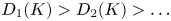$D_1(K)>D_2(K)>\ldots$, and the corresponding eigenvectors form an orthonormal basis. Eigenvalue $D_1(K)$ as a function of the wavelength $\lambda =2{\rm \pi} /K$ is shown in figure 3(a), with a few representative eigenvectors shown in figure 3(b). Note how, as $K$ increases, the region over which the eigenvector is non-negligible decreases. In fact, with a simple rescaling of the problem, it can be shown that the extent of the non-zero region decreases as $1/\sqrt {K}$. Although it is not possible to give an analytic expression for $D_m$, we have $D_m(K)= O(K^2)$ for $K\ll 1$, whereas 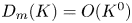$D_m(K) = O(K^0)$ for $K\gg 1$. In particular, the fact that the eigenvalues saturate at large wavenumbers will have significant consequences. For a given horizontal wavenumber $K$, substituting (5.2) into (5.1) yields a system of coupled ordinary differential equations for the amplitude functions $f^K_m(t)$. In Appendix B we show that when the Reynolds number is large (with fixed Prandtl number), to leading order the system decouples, so that each amplitude function $f^K_m(t)$ evolves independently from the other. For a given $f^K_m(t)$, the inviscid growth rate is controlled by the eigenvalue $D_m(K)$. Because we are interested in the characteristics of the fastest growing perturbations, we focus on the case $m=1$. From now on, $D(K)=D_1(K)$ and $f^K(t)=f^K_1(t)$. By introducing the renormalised wavenumber $\mathfrak {K}=K/\sqrt {DRe}$, to order $O(Re^{-1/2})$ the amplitude $f^{\mathfrak {K}}(t)$ satisfies the following equation:

(5.5)\begin{equation} \frac{{\rm d}^2f^{\mathfrak{K}}}{{\rm d}t^2}+\mathfrak{K}^2\left(1+\frac{1}{Pr}\right)\frac{{\rm d}f^{\mathfrak{K}}}{{\rm d}t}+ \left(Pr^{{-}1}\mathfrak{K}^4-D(K)\frac{t^n}{n!}\right)f^{\mathfrak{K}} =0, \end{equation}

where $Pr=Pe/Re$ is the Prandtl number of the fluid.

Figure 3.

Solution of the Sturm–Liouville problem (5.3a,b). (a) Eigenvalue $D$ as a function of $\lambda$. (b) Eigenvector $\phi (z)$ for the maximal $D$ for a given $\lambda$. Solutions are obtained by solving (5.3a,b) using a domain $-5 \leq z \leq 0$, boundary conditions $\phi (-5)=\phi (0)=0$ and 1000 uniform grids. The eigenvalue $D$ controls the growth rate in (5.8)–(5.9), (5.14) and (5.17), while the eigenvector $\phi (z)$ represents the vertical structure of perturbations.

In the previous equation, we can discern two limits. In the limit $\mathfrak {K}\to \infty$ with $Re$ constant, (5.5) tends to a simple differential equation with constant coefficients, whose characteristic polynomial has roots

(5.6)\begin{equation} \sigma^\infty_{1,2}(\mathfrak{K})={-}\mathfrak{K}^2\{1,Pr^{{-}1}\}, \end{equation}

both of which are real and negative and thus exponentially damped. This is to be expected on physical grounds, as for sufficiently small wavelengths diffusive effects will smooth out and eventually dampen fluctuations. Conversely, when $\mathfrak {K}\to 0$, with $K$ constant, the equation reduces to the modified Airy equation:

(5.7)\begin{equation} \frac{{\rm d}^2f^{0}}{{\rm d}t^2}-D(K)\frac{t^n}{n!}f^{0}=0, \end{equation}

whose solution grows asymptotically as

(5.8)\begin{equation} f^{0}(t) \sim \frac{1}{D(K)^{1/12}t^{1/4}}{\rm e}^{(\sigma_t t)^{3/2}}, \quad \sigma_t=\left(\frac{2}{3}\right)^{2/3}D(K)^{1/3}, \quad \text{as} \ t \gg 1, \end{equation}

when $n=1$ and as

(5.9)\begin{equation} f^{0}(t) \sim \frac{2^{3/8}}{D(K)^{1/8}t^{1/2}}{\rm e}^{(\sigma_d t)^2}, \quad \sigma_d=\frac{D(K)^{1/4}}{2^{3/4}}, \quad \text{as} \ t \gg 1, \end{equation}

when $n=2$. In practice, these asymptotic formulas apply already for $t=O(1)$, as seen by comparing asymptotic solutions with the numerical integration of the corresponding equations (figure 4). Note that $\sigma _d$ and $\sigma _t$ tend to saturate as $K\to \infty$, whereas the viscous damping time scale becomes increasingly shorter. On physical grounds, we can thus expect that at a certain wavenumber, dependent on the Reynolds number, a cross-over occurs whereby viscous damping dominates and so very little energy should be found above such a wavenumber. To verify our intuition, we consider the general solution of (5.5). It can be written in terms of special functions.

Figure 4.

Comparison between asymptotic solution and numerical solution using a third-order Runge–Kutta (RK3) method with ${\rm d}t = 0.01$, and initial conditions $f(0) = 1$ and $f'(0) = 0$. The comparison is to show that the asymptotic solution captures the growth of the numerical solution as $t \gg 1$. Solid curves are for $D = 1$; dashed for $D = 0.5$. (a) Asymptotic solution (5.8) and numerical solution of the modified Airy equation (5.7) with $n=1$. (b) Asymptotic solution (5.9) and numerical solution of (5.7) with $n=2$.

5.1. Time-independent radiation

We consider first the case when $n=1$. In this case we have

(5.10)\begin{equation} f^{\mathfrak{K}}(t)=c_1(\mathfrak{K})A(\mathfrak{K},t)+c_2(\mathfrak{K})B(\mathfrak{K},t). \end{equation}

Here $c_1(\mathfrak {K})$ and $c_2(\mathfrak {K})$ are integration constants and the functions $A$ and $B$ can be expressed in terms of Airy's Ai and Bi functions

(5.11)\begin{equation} \left.\begin{gathered} A(\mathfrak{K},t)={\rm e}^{\bar{\sigma}(\mathfrak{K})t} {\rm Ai}(\zeta(\mathfrak{K},t)), \quad B(\mathfrak{K},t)={\rm e}^{\bar{\sigma}(\mathfrak{K})t} {\rm Bi}(\zeta(\mathfrak{K},t)), \\ \zeta(\mathfrak{K},t)=\frac{(1-Pr^{{-}1})^2\mathfrak{K}^4+4D(K)t}{4D(K)^{2/3}}, \end{gathered}\right\} \end{equation}

and $\bar {\sigma }(\mathfrak{K})$ is the arithmetic mean of $\sigma ^\infty _i(\mathfrak {K})$. The integration coefficients are given by

(5.12)\begin{equation} c_1(\mathfrak{K})=\frac{(\bar{\sigma}(\mathfrak{K})-1)\,{\rm Bi}(\zeta(\mathfrak{K},0))f'(0)+ {\rm Bi}'(\zeta(\mathfrak{K},0))f(0)}{\varDelta(\mathfrak{K})} \end{equation}

and

(5.13)\begin{equation} c_2(\mathfrak{K})={-}\frac{(\bar{\sigma}(\mathfrak{K})-1)\,{\rm Ai}(\zeta(\mathfrak{K},0))f'(0)- {\rm Ai}'(\zeta(\mathfrak{K},0))f(0)}{\varDelta(\mathfrak{K})}, \end{equation}

with $\varDelta (\mathfrak {K})={\rm Ai}(\zeta (\mathfrak {K},0)\,{\rm Bi}'(\zeta (\mathfrak {K},0))- {\rm Ai}'(\zeta (\mathfrak {K},0)\,{\rm Bi}(\zeta (\mathfrak {K},0))$.

For $t>1$ the solution can be asymptotically expressed as

(5.14) \begin{equation} \left.\begin{gathered} f^{\mathfrak{K}}(t) \sim {\rm e}^{\varSigma_t t} \left[\mathfrak{K}^4\left(\frac{Pr-1}{Pr}\right)^2+4Dt\right]^{{-}1/4},\\ \varSigma_t={-}\frac{\mathfrak{K}^2}{2}\left(\frac{1+Pr}{Pr}\right)+\frac{1}{12Dt}\left[\mathfrak{K}^4\left(\frac{Pr-1}{Pr}\right)^2+4Dt\right]^{3/2}\\ -\frac{1}{12Dt}\left[\mathfrak{K}^4\left(\frac{Pr-1}{Pr}\right)^2\right]^{3/2}. \end{gathered}\right\} \end{equation}

The solution when molecular viscosity and diffusivity are equal ($Pr=1$) is particularly illuminating, since in this case the solution is simply the inviscid solution multiplied by the viscous damping term:

(5.15a,b)\begin{equation} f^{\mathfrak{K}}(t)\sim \frac{1}{D(K)^{1/12}t^{1/4}}\exp({-\mathfrak{K}^2t+(\sigma_t t)^{3/2}}), \quad \sigma_t=\left(\frac{2}{3}\right)^{2/3}D(K)^{1/3}. \end{equation}

Neglecting the (weak) algebraic dependence on time of the prefactor, we see that evolution of a perturbation with a horizontal wavenumber $K$ is controlled by the time- and wavenumber-dependent growth rate:

(5.16)\begin{equation} \varSigma_t = \frac{1}{Re}\left(-\frac{K^2}{D(K)}+\frac{2}{3}\sqrt{D(K)tRe^2}\right). \end{equation}

Figure 5(a–c) shows the growth rate for a range of times as a function of the wavelength. Note that $\varSigma _t$ is at most $O(1)$, which vindicates the choice of $t_0$ as the relevant time scale for the process.

Figure 5.

Asymptotic growth rate $\varSigma$ versus wavelength at different times. The vertical red lines indicated the estimated high-frequency cut-off $\mathfrak {K}=1$, i.e. $\lambda \sqrt {Re} \approx 2{\rm \pi}$. (a–c) Steady radiation. (d–f) Diurnal radiation.

For a given $Re$, there is a Reynolds-number-dependent $t_{min}$ such that for $t< t_{min}$ the time-dependent growth rate $\varSigma _t(K,t)<0$. This can be easily seen considering that as a function of $K$ the viscous damping is a convex function which tends to a value $O(1/Re)$ for $K\to 0$, whereas the inviscid growth is a concave function which approaches zero as $K\sqrt {t}$ for small values of $K$ (figure 6).

Figure 6.

Viscous damping and inviscid growth rate as a function of wavelength under steady radiation conditions. The viscous damping is time-independent, whereas the inviscid growth rate accelerates with time. Up to $t\sim 481Re^{-2}$, viscous damping dominates. Past this time, a widening range of wavenumbers experiences net growth.

To find how $t_{min}$ depends on $Re$, we consider the following ansatz: $t_{min}=\beta Re^{-2}$. When substituted into (5.16), the Reynolds number is factored out, leaving an equation for $\beta$ that can be easily solved numerically. We obtain $\beta \simeq 491$ and a Reynolds-independent marginal wavelength $\lambda _{mar}\simeq 10.7$. Past $t_{min}$ the range of wavelengths that experiences growth widens. The upper limit of the range increases as $Re\sqrt {t-t_{min}}$. The lower limit of the range decreases as $Re^{-1/2}(t-t_{min})^{-1/4}$. The peak of the growth rate rapidly shifts to smaller wavelengths (figure 5a–c). The existence of a minimum time that needs to elapse before instabilities can grow implies that instabilities will appear only after the background stratification has grown sufficiently. Since the non-dimensional time-dependent background stratification is $N^2=-t\textrm {e}^{z}$, the minimum near-surface background stratification necessary to sustain perturbations is $-t_{min}$.

However, we recall that the superexponential growth given by (5.16) is not expected until $t\simeq 1$. Therefore, for large values of the Reynolds number, by the time the solution enters the superexponential phase, a range of wavelengths is already poised to grow. Moreover, for large values of $Re$, the growth rate for most wavelengths experiencing growth is only weakly dependent on the Reynolds number. Only wavelengths that are close to either side of the interval see a significant departure from purely inviscid growth. Thus, when comparing our results with numerical simulations, we use the inviscid limit.

The asymptotic expression is more complicated when $Pr\neq 1$, but as long as $Pr$ remains finite, there is no qualitative change in the behaviour of the solution and little quantitative change. In fact, as we shall see, the predicted growth rate and peak wavelength at $Pr=1$ match the values observed in the numerical simulation at $Pr=10$.

The above analysis suggests that instabilities will always appear, provided that enough time is allowed for the stratification to reach its critical value, regardless of the magnitude of the Reynolds number. However, as we remarked above, (5.5) was derived in the large-$Re$ limit. Superexponential growth requires $t_{min}$ to be ${\simeq }1$ or larger. For values of $Re$ greater than 20, by the time the superexponential phase begins, there is already a range of wavelengths with positive growth rates. Whether values of $Re$ smaller than 20 can still be considered ‘large’ for the purpose of the theory remains to be seen. It is certainly reasonable to assume that no matter how small the Reynolds number is, a sufficiently large accumulation of negative buoyancy at the surface should be able to overcome the stabilising effect of viscosity and diffusion, but this is a question that our theory cannot answer with certainty. Moreover, our theory works in the small-$\tau$ limit. Under highly diffusive conditions, the growth of the surface boundary layer cannot be neglected.

5.2. Diurnal solar radiation

For the diurnal radiation case ($n=2$), the general solution to (5.5) can be expressed in terms of a combination of Hermite polynomials and hypergeometric functions, which play the role of Airy's functions for the $n=1$ case. In this case, it is the hypergeometric function that dominates the behaviour for large values of $t$. For large $t$ the asymptotic solution is

(5.17) \begin{align} \left.\begin{gathered} f^{\mathfrak{K}}(t) \sim c_2(\mathfrak{K}) {\rm e}^{\varSigma_d t} \left[\sqrt{2D}t+\sqrt{\mathfrak{K}^4 \left(\frac{Pr-1}{Pr}\right)^2+2Dt^2}\right]^{{\mathfrak{K}^4}/{(32D)^{1/2}}\left({(Pr-1)}/{Pr}\right)^2}\\ \times\left[\mathfrak{K}^4\left(\frac{Pr-1}{Pr}\right)^2+2Dt^2\right]^{{-}1/4}, \\ \varSigma_d={-}\frac{\mathfrak{K}^2}{2}\left(\frac{1+Pr}{Pr}\right)+\frac{1}{4}\left[\mathfrak{K}^4\left(\frac{Pr-1}{Pr}\right)^2+2Dt^2\right]^{1/2}, \end{gathered}\right\} \end{align}

where in this case $c_2(\mathfrak {K})$ is the coefficient of integration associated with the hypergeometric function. The growth rate $\varSigma _d$ is dependent on time and wavenumber, which, when $Pr=1$ can be written as (figure 5d–f)

(5.18)\begin{equation} \varSigma_d=\left(-\frac{K^2}{D(K)Re}+\frac{\sqrt{D}t}{2\sqrt{2}}\right). \end{equation}

Relative to the steady radiation case, the growth is more gradual at the onset, and steeper at later times, but the pattern is otherwise very similar.

In this case as well the background stratification must grow beyond a $Re$-dependent critical threshold for instabilities to grow. The analysis is very similar to the one done for the steady radiation case, with the exception that now $t_{min}\simeq 42Re^{-1}$ has the same value for the marginal stability wavelength. The upper limit of the unstable range increases as $Re\,t$, whereas the lower range decreases as $(Re\, t)^{-1/2}$ (figure 5d–f).

6. Comparison with numerical simulations

To validate the theory developed in the preceding section, we use the Stratified Ocean Model with Adaptive Refinement (SOMAR) to compare the prediction of our theory with the DNS simulations of RDC. SOMAR solves the Navier–Stokes equations under the Boussinesq approximation (Santilli & Scotti Reference Santilli and Scotti2015; Chalamalla et al. Reference Chalamalla, Santilli, Scotti, Jalali and Sarkar2017) using an operator splitting technique. The finite-volume discretisation is second-order in space, while a third-order Runge–Kutta method is adopted for time marching. The Poisson equation is solved with an efficient multigrid solver. SOMAR adjusts the time step based on a Courant–Friedrichs–Lewy (CFL) condition to maintain stability under advection. Viscous terms are treated implicitly.

We solve (2.1) and (2.2) in a rectangular domain extending from the surface to the bottom. Equations are discretised with uniform grids in each direction. The initial condition is a motionless, unstratified fluid plus perturbations of two types. The first type is initialised with single-mode perturbations with the most unstable wavelength predicted by (5.14) and (5.17) and the corresponding vertical structure shown in figure 3(b), with the peak normalised by $W_0$ being 0.001. The second type is initialised with random temperature perturbations (normalised by $T_0$) uniformly distributed in the range $-0.01$ to 0.01 over the entire domain. The boundary conditions are periodic in the horizontal direction. At the surface and at the bottom of the domain we use free-slip conditions and zero buoyancy flux. The use of free-slip conditions at the bottom removes the need to resolve the viscous sublayer. As convective activity is mostly confined with $Z_0$, the effect is negligible at large Reynolds numbers.

The range of random temperature perturbations ($-0.01$ to 0.01) is chosen so that nonlinear terms are at least two orders of magnitudes smaller than linear terms. The effect of the magnitude of random perturbations is examined in Appendix D.

The configuration of all cases simulated and compared with the theory is described in table 1. Cases TLR and THR consider time-independent radiation. The other two cases, DLR and DHR, consider periodic radiation conditions. The non-dimensional parameters in the time-periodic cases correspond to typical values found in Lake Onego (DLR) and Lake Michigan (DHR).

Table 1.

Configurations for the numerical simulations considered in §§ 5.1 and 5.2. For each simulation, we list the Reynolds number $Re = W_0 Z_0/\nu$, the Péclet number $Pe=W_0Z_0/\kappa$, the ratio $\delta /S$ of the thickness of the viscous surface layer at $\tau =1/Pe$ to the thickness of the most unstable mode $S$, time scale ratio $t_0\varOmega$, the eigenvalue of the most unstable mode $D$, the wavelength of the most unstable mode $\lambda _p$, the vertical extent (measured from the surface) of the most unstable mode $S$, the number of grid points $N_h$ that resolve one horizontal wavelength and the number of grid points $N_v$ that resolve $S$ in vertical. All lengths are measured in units of $Z_0$. In all the cases considered, the non-dimensional depth $H$ of the domain is 5.

Together, these four cases cover a wide range of $Re$ from 200 to 65 000 with $Pr=10$, which is typical for freshwater below the critical temperature. From our theory, we expect that over such a range of Reynolds numbers, the critical wavelength and vertical structure should vary appreciably. To capture these characteristics in each case, the choice of grid spacing is made with the following criteria in mind. First, the vertical domain is 5 times $Z_0$, and horizontal domain is sized to contain 100 wavelengths with the highest growth rate $\lambda _p$. Second, at least 161 horizontal grid points resolve the wavelength with the highest growth rate $\lambda _p$ and at least 40 grid points resolve the cut-off wavelength $\lambda _{cut}$. In the vertical we use at least 122 grid points to resolve the sharp vertical variation $S$ near the surface (see $\lambda _p$, $S$, $N_h$ and $N_v$ in table 1). Third, and finally, in addition to the CFL condition necessary to ensure the numerical stability of the scheme, the time step is further subject to the constraint that it should not exceed $t_0/40$. These three rules ensure that the numerical set-up does not bias the simulations. Sensitivity to grid resolution tests is reported in Appendix C.

To distinguish between the linear stage (where our theory is expected to hold) and the nonlinear stage we compare $\partial b/\partial t$ and $w(\partial b/\partial z)$ in the buoyancy equation and $\partial w/\partial t$ and $w(\partial w/\partial z)$ in the $z$-momentum equation. We compute the root mean square (r.m.s.) of each term for comparison. The average is taken over the vertical range in which the eigenfunction of the most unstable wavelength varies ($S$ in table 1 and figure 3b). The theoretical solution is normalised so that at $t=2$ it coincides with the numerical solution.

6.1. Time-independent radiation

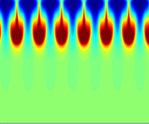
Case TLR initialised with single-mode perturbations is shown in figure 7(a). The leftmost column displays the time evolution of the horizontally averaged buoyancy. The red curve shows the value assumed by the theory, while the blue dashed line is calculated from the SOMAR output. The two profiles are still identical at $t=6$, while significant difference exists at $t=7$, signalling the end of the linear stage. Even towards the end of the linear stage, the energy is still concentrated at the wavelength of the initial condition (last column). Buoyancy and vertical velocity are shown in the central columns. The perturbations evolve as a series of downward localised jets.

Figure 7.

Evolution of RDC under time-independent radiation profile, with $Re=932$ and single-mode perturbations. (a) From rows 1 to 3, time advances. Column 1: comparison between theoretical basic state buoyancy $\bar {b}(z,t)$ and horizontally averaged buoyancy profile $b_{ave}$. Column 2: side view of total buoyancy $\tilde {b}$. Column 3: side view of perturbation buoyancy $b$. Column 4: side view of vertical velocity, which is also perturbation vertical velocity $w$. Column 5: vertical velocity spectrum at $z=-1$, $-2/3$ and $-1/3$. Wavelength $\lambda$ is the wavelength of the perturbations, $\lambda _p$ represents the theoretical most unstable wavelength and $\lambda _{cut}$ the theoretical cut-off wavelength. Note the appearance of a spectral line at half the forcing wavelength due to the quadratic term in the equation of motion at $t=5$. Only when the flow becomes fully nonlinear do we observe energy at wavelengths smaller than $\lambda _{cut}$. (b) The r.m.s. of linear and nonlinear terms in the legend and $\textrm {d}f^{\mathfrak {K}}(t)/\textrm {d}t$ and $\textrm {d}f^{0}(t)/\textrm {d}t$ as a function of time. Wavelength $\lambda _p$ is calculated from (5.14), and $D$ is computed via (5.3a,b). (c) Growth rate as a function of time. The red curve is computed from the SOMAR output. The green curve is the theoretical value (5.14).

The growth of the perturbations in the simulation agrees well with that predicted by the theory until the magnitude of the nonlinear terms catches up with the magnitude of the linear terms around $t=6.7$ (figure 7b).

We estimate the time-dependent growth rate from the simulation as

(6.1)\begin{equation} \varSigma_t\approx \frac{2}{3}\frac{{\rm d}}{{\rm d}t}(\ln \tilde{w}), \end{equation}

which compares extremely well with the theoretically predicted value (figure 7c) from $t=3$ to $t=6$, after which the former declines because the system approaches the nonlinear stage. The discrepancy at earlier times may simply indicate that (6.1) is sensitive to small change in $w$, since $\partial w/\partial t$ and $\textrm {d}f^{\mathfrak {K}}(t)/\textrm {d}t$ agree well (figure 7b). Note that over the interval $t=2$ and $t=6$ the magnitude of the perturbation grows by three orders of magnitude.

Between $0 < t < 1$, $\partial w/\partial t$ drops slightly (figure 7b). Presumably, during this time, viscosity in (2.9) and diffusivity in (2.10) play a role in the evolution of perturbations, because $\partial \bar {b}/\partial z$ in (2.10), which grows from 0, is not strong enough. This does not contradict the balance (4.1) and (4.2) and the subsequent analysis in §§ 4 and 5. Equations (4.1) and (4.2) target the evolution of perturbations when $\partial \bar {b}/\partial z$ grows continuously, and the analysis which follows applies for $t>1$.

Simulations of case TLR with white-noise perturbations are shown in figure 8. The major difference in this case is that the spectrum contains energy over the range of wavelengths that experience positive growth, peaked on the wavelength of maximal growth ($\lambda _p=0.6$ at $Re=932$) predicted by the theory, which also predicts well the vertical envelope of the perturbations, with a peak at $z=-0.25$ (figure 3b). Towards the end of the linear stage, there is a shift of the spectrum to larger wavelengths, likely due to the nonlinear merger of plumes. Of course, in the nonlinear stage three-dimensional effects become dominant, which are not captured by our simulations. The spectra at different depths essentially overlap, indicating strong coherence across the vertical dimension, consistent with a single mode being energised.

Figure 8.

Same as figure 7 but with white-noise perturbations.

Overall, the theory predicts well how the perturbation grows in time, though the measured time-dependent growth rate $\varSigma _t$ is somewhat smaller than that calculated from the theory, though the latter is the growth rate expected from the most unstable mode, whereas in the simulation we have a combination of modes across a range of horizontal wavenumbers that, while following the same growth pattern, have different values of the eigenvalue $D(K)$. Thus it is to be expected that the measured $\varSigma _t$ be lower than the theoretical value based on the most unstable wavelength.

Case THR considers a much larger value of the Reynolds number ($Re=65\,444$). In this case as well the averaged numerical buoyancy profile agrees well with the profile used for the theoretical analysis up to $t=5.5$, after which the numerical solution becomes dominated by nonlinearity (figure 9a, column 1). The spectra at different depths do not exactly overlap, as was the case at lower values of the Reynolds number, though still peaking near the expected wavelength of maximal growth ($\lambda _p=0.1$). At large values of the Reynolds number, the growth rate of higher vertical modal orders is less sensitive to the modal number, and therefore we expect that the flow initialised with random perturbations will exhibit a mixture of contributions from different modes. Overall, the theory captures well the growth of the perturbations (figure 3b), though the presence of a continuum of energised wavelengths is reflected in the overall time-dependent rate of growth, which, while following the expected increase in time between $t=2$ and $t=4.5$ is lower than the growth rate based on the most unstable wavelength and mode (figure 9c).

Figure 9.

Same as figure 7, but with $Re=65\,444$, white-noise perturbations and smaller colourbar range for columns 1–4.

6.2. Diurnal solar radiation

Simulations forced by diurnal solar radiation with single-mode perturbations agree well with theory, as was the situation for case TLR in the preceding section. Therefore, in this section we focus on simulations with white-noise perturbations.

Case DLR uses parameters typical of springtime conditions in a shallow temperate lake (Lake Onego; Bouffard et al. Reference Bouffard2019). Compared with the other cases considered, diffusion effects are stronger, which results in a relatively low value for the Reynolds number ($Re=196$). The agreement between the buoyancy profile computed from the simulation and that used in the theory is good up to $t=6$, after which nonlinearity dominates (first column in figure 10a; also figure 10b indicates that the nonlinearity begins at $t=6.6$). The spectra at $t=5$ peak near $\lambda \approx 1.2$, close to the theoretical prediction $\lambda _p=1$. Beginning at $t=6$ we observe a shift of the energy to longer wavelength. This may be due to the flow becoming more nonlinear. At $\lambda _p=1$ the corresponding mode-1 structure function (figure 3b) extends to $z=-1.7$, with a peak at $z=-0.4$, which captures well the vertical envelope of the fluctuations. The growth of the r.m.s. fluctuations is well described by the theory (figure 10b). Over $2 \leq t \leq 6.6$, the amplitude of the fluctuations increases by four orders of magnitude. Setting $\tilde {w}=\exp (\sigma t^2)$ we compute the growth rate $\varSigma _d=\sigma t$ as

(6.2)\begin{equation} \varSigma_d \approx \frac{1}{2}\frac{{\rm d}}{{\rm d}t}(\ln\tilde{w}). \end{equation}

The computed growth rate is in good agreement up to $t=6.2$ (figure 10c), after which the computed growth rate declines as the linear and nonlinear terms become comparable (figure 10b). As was for the steady radiation cases, the calculated growth rate when the flow is initialised with a spectrally broad-banded initial condition is somewhat lower than the theoretically predicted value. However, the trend in time is very similar, and the same considerations that we presented in the steady radiation case apply here as well. Overall, the agreement between theory and simulations is good.

Figure 10.

Radiatively driven convection under time-dependent radiation at $Re=196$ initialised with white noise. Symbols and colours as in figure 7. Note that the colourbar range for columns 1–4 is greater.

Case DHR is representative of a deeper lake, close to critical temperature on a cloudy day. Such conditions are often observed in Lake Michigan and Lake Superior (Austin Reference Austin2019; Cannon et al. Reference Cannon, Troy, Liao and Bootsma2019). With the role of viscosity and diffusivity diminished, the superexponential growth rate is larger, and therefore the duration of the linear phase is shorter. Prior to $t=5$, the theoretical basic state buoyancy (4.6) and SOMAR output coincide, after which nonlinearity becomes apparent ($t=5.5$) (figure 11a, column 1). The spectra peak around the theoretical wavelength of maximal growth ($\lambda _p=0.15$), which is almost an order of magnitude shorter than in the previous case. The vertical envelope of the fluctuations is confined in the upper 10 % of the water column during the linear phase, as expected from the mode-1 function associated with $\lambda _p$. The computed time-dependent growth rate follows the theoretical profile well, though it is smaller than the value expected for the the wavelength of maximal growth. Again, this is to be expected, since the range of active wavenumbers is wide.

Figure 11.

Radiatively driven convection under time-dependent radiation profile at $Re=20\,908$ with white-noise initial condition. Symbols and colours as in figure 7. Note that the colourbar range for columns 1–4 is smaller.

7. Summary and conclusions

We have considered the characteristics of the perturbations at the onset of RDC. In this stage, the perturbations are small enough that it is permissible to linearise the equations of motions around a quiescent background state characterised by a time-varying buoyancy profile. We considered both steady radiation, which has been considered in recent laboratory experiments (Bouillaut et al. Reference Bouillaut, Lepot, Aumaître and Gallet2019) and has applications to stellar interiors (Kippenhahn, Weigert & Weiss Reference Kippenhahn, Weigert and Weiss1990), as well as time-dependent cases, more representative of RDC in temperate lakes during springtime and which may have application to atmospheric convection (see e.g. figure 4 in Deardorff (Reference Deardorff1974)). As opposed to the more traditional Rayleigh–Bénard convection, where the background state moves heat at fixed rate from bottom to top boundary, while remaining constant in time, in RDC the background state evolves in time, as heat is continuously added by radiation, and only after the onset of convection can heat be effectively redistributed in the interior. By considering the most likely balance in the dynamical equations, we build velocity and time scales which together with viscosity allow the definition of a Reynolds number. We develop a theory that is valid for large values of the Reynolds number that predicts the wavelength, vertical structure and growth rate of the perturbations during the initial linear stage. Due to the time-dependent nature of the background state, the growth of perturbations not significantly affected by viscous damping has the form $\exp [(\sigma t)^n]$, where the exponent is $n=3/2$ for time-independent radiation and $n=2$ for diurnal radiation. We have confirmed the analysis by comparison with highly resolved DNS.

The theory gives a way to estimate the duration of the linear phase. Indeed, the latter terminates when the amplitude of the nonlinear terms becomes comparable to the amplitude of the linear terms. In Appendix D we show that the duration of the linear phase over a range of intensities of the residual flow at dawn is found to be between $3t_0$ and $6t_0$, where the linear time scale $t_0$ is given by the last of (4.7a–c). For Lake Superior, assuming a water temperature of $T=3.5\,^\circ \textrm {C}$ and an $e$-folding scale $Z_0=10$, we obtain $t_0 \approx 80$ min on a cloudy day when the radiative intensity is $So \approx 200\ \textrm {W}\ \textrm {m}^{-2}$. On a sunny day, with the radiative intensity $So \approx 800\ \textrm {W}\ \textrm {m}^{-2}$, the linear time scale is reduced to $t_0 \approx 60$ min.

If we accept that once turbulence sets in the vertical gradient in temperature stabilises, the latter is then set by the length of the linear phase. Ceteris paribus, a weaker initial circulation left over from the previous cycle will result in a longer linear phase and thus a stronger stratification at the onset of the turbulent phase, that is, a stronger temperature contrast upon which advection acts. This should result in larger r.m.s. temperature fluctuations (relative to the background) during the day. With lakes as our geophysical example of RDC under periodic radiation forcing, one way to test this prediction from an observational point of view would be to correlate the strength of the fluctuations in temperature to the strength of the residual circulation at first daylight.