STUDY REGION AND SEISMIC DEPLOYMENT

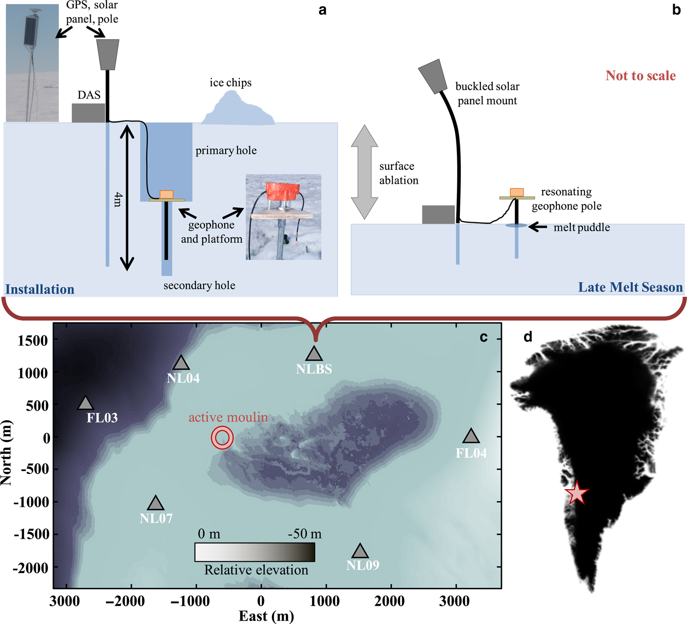
Following observations of a supraglacial lake drainage via a moulin in 2006, we deployed seismic, GPS receivers and temperature loggers onto the GrIS (68.73°N, 49.53°W, Fig. 1) each year, over multiple years (2007–2012), to record any ice deformation, hydraulic signatures, and speedup that accompanied the drainage of supraglacial lakes that (nearly) colocated with the lake that drained in 2006 (hereon termed ‘North Lake’). The seismic sensors included 4.5 Hz, triaxial L-28 geophones that continuously logged data at 200 s⁻¹. The network geometry for each seismic deployment near the North Lake varied yearly, but consistently included a base station site (NLBS). Starting in 2009, deployment teams reinstalled NLBS and additional geophones using a ‘pole and platform’ assembly, intended to sustain sensor orientation and ice–instrument coupling. To perform this installation, we mounted L-28 geophones upon small plywood platforms that we drilled to accept L-28 geophone pegs and 3 cm diameter, 1.6 m long hollow-core aluminum poles that secured each geophone. We installed these mounts within 0.5 m-diameter, 2 m deep holes that we cored into the snow-free ice at each site. Each geophone platform pole fit into a 6 cm diameter, secondary hole that we cored to an additional depth of 2 m at the bottom center of each primary hole. This configuration allowed the geophone platform to rest on the bottom of the primary hole (Fig. 1, top left). We then oriented the geophone to true north, leveled it and tamped the platform down. Last, we back-filled the primary hole with ice chips and ran diagnostics upon the cumulative data acquisition system (DAS) before we left the field site unsupervised.

Fig. 1.

(a) Cartoon of the NLBS geophone-pole-platform, GPS pole and solar panel mount assemblies installed into the Western GrIS surface, in snow-free conditions. (b) Same instrument deployment after melt-out; DAS refers to the digitizer, data logger and battery. (c) A subset of the 2011–2012 seismic and GPS instrument co-deployment, superimposed on a DEM image of the Western GrIS lake basin near the North Lake, after it drained on DOY 169, 2011 through the labeled moulin. The center of the seismic network marks the origin of a local coordinate system, and color scale approximately marks the highest elevation features (1025 m, dark) versus the lowest elevation features (975 m, light). (d) The geographical location of the lake site (68.73° N, 49.53° W, red star).

SPECTRAL FEATURES OF DATA

We recovered geophone data loggers from NLBS and six other sites during a 2012 site visit (station SLAKE off-map in Fig. 1). To search for harmonic signals ostensibly related to hydraulic forcing, we computed long-term, bandlimited (0-50 Hz) spectrograms from each channel of our velocity data with a 150 s sliding window that we zero padded to 300 s, overlapped by 50% and tapered with a Hamming window. These spectrograms revealed narrowband features of seismic energy elevated over background noise that became visible in the late melt season (July, 2011) after the North Lake drained on day of year (DOY; 169, 2011) (Fig. 2, top). Each feature appeared as bright curves in time-frequency space that trended with decreasing frequency, over recording duration into the melt season. To better reveal these spectral features, we modified and applied a spectral peak detector (Taylor and others, Reference Taylor, Arrowsmith and Anderson2010) to estimate extreme value statistics of our spectrograms over time. In summary, this detector (1) processed each spectrogram in a sliding time window, (2) retained all spectral amplitudes ≥ 0.9 × the peak spectrogram value, per window, and (3) assigned the threshold-exceeding statistics to this peak bin value (per 800 s bin). The detector then assigned the remaining data marked by spectral amplitudes <0.9× the bin maximum, to zero. This process produced a binary map (a bit-map) that effectively performed an automatic gain control on the spectra. This resultant bit-map clearly exposed the oscillatory, narrowband features within our data between 12 Hz ≤ ξ ≤ 35 Hz that fluctuate in peak frequency over diurnal cycles (Fig. 2, bottom). On time scales of several days, the curve troughs of these oscillatory features that indicated high seismic power coincided with expected peak melt. Conversely, curve peaks coincided with expected minimum melt. Such features generally show increased spectral power at lower frequencies as the melt season progressed. Data recorded on the NLBS station exhibited multiple narrowband features as bright lines or curves simultaneously. These same features disappeared or became muted later into the melt season, as solar exposure and temperatures decreased.

Fig. 2.

(a) A velocity spectrogram computed from NLBS.ELE (East channel) data over the 2011 melt season (0–50 Hz). The inset scatter plot shows that transverse (North–South) vibrations dominate geophone records during resonance (DOY 220). (b) Detected spectrogram peaks superimposed with beam and rod eigenfrequencies (Equation 1 and Equation 3). Mismatch between modeled resonance and spectral features likely reflect inaccurately modeled ablation, geophone burial depth and geophone pole stiffness. Measured diurnal oscillations in spectral peaks likely indicate a lengthening and shortening of the geophone pole by a melting and refreezing of a puddle at the pole base. Higher frequency features apparent after DOY 225 have unknown sources.

When viewed in isolation, spectral features recorded by our geophones resemble some features of glaciogenic tremor documented elsewhere (Podolskiy and Walter, Reference Podolskiy and Walter2016, Fig. 7). Data collected 85 km south of North Lake, for example, show that geophones deployed hundreds of meters from a moulin also record high-power, narrowband signals that measure water column resonance (an ‘organ pipe’) within a partially filled moulin, that is excited by a waterfall impacting the water surface, inside that moulin (Röösli and others, Reference Röösli, Walter, Ampuero and Kissling2016). The frequency content (~ 5 Hz) of the spectra recorded by Röösli and others was consistent between geophones and showed amplitude decay with geophone distance from the moulin. Our data do not show consistency in the timing of spectral peaks at separate geophone locations (Carmichael and others, Reference Carmichael2015, Fig. 2). This inconsistency requires separate sources for the narrowband signals. To compare our analysis with this previously published North Lake data, we focus mostly on spectra derived from NLBS geophone records (also see Geophone NLBS Data Spectrograms in our Electronic Supplement).

GEOPHONE POLE RESONANCE IMPRINTS ON SPECTROGRAMS

We now consider a non-glaciogenic source of the spectral peaks in our data that relates to geophone installation: over the course of the 2011 summer season, several meters of surface ice near the North Lake ablated and subsequently exposed each buried geophone (Fig. 1, top right). Additional surface melt then exposed a length L of each geophone pole that grew with ablation rate. The solar panel system adjacent to each geophone installation site that provided the DAS power also melted out, and provided a longer record of net surface ablation at each site.

To determine the effect of this melt-out on the transverse vibrational excitation of a geophone, we model a geophone pole as a cantilevered beam of length L supporting a small point mass dm under gravity g. We further suppose this instrumented end forms an axial load (dm)g on the pole, where the instrumented end is unconstrained, and the bottom end forms a pinned boundary condition. The instrumented pole model resembles an Euler–Bernoulli beam susceptible to buckling and vibrational resonance through bending oscillations at particular eigenfrequencies that satisfy the fourth-order beam equations of motion. The eigenfrequencies ξ_i (Hz) of such a free-pinned system approximate (Segel, Reference Segel2007, p. 518–520):

(1)$${\rm \xi }_i^{({\rm Beam})} = \displaystyle{1 \over {2\pi }}\displaystyle{{L_i^2 } \over {L^2}}\sqrt {\displaystyle{{EI} \over {{\rm \rho }A}}} ,\quad i = 1,2, \ldots $$

In Equation 1, L (units m) linearly relates to the ice surface ablation rates over time scales much greater than a vibrational period, L ₁ = 1.86 m when unitless integer i=1 (eigenmode 1). Quantities E, I, A and ρ respectively represent Young's modulus of the pole, the moment of inertia about the fixed end, the effective cross-sectional area of the pole and the effective pole density. Term $\sqrt { {E I}/{\rho A}}$ depends upon unknown factors that influence effective pole stiffness, like ice content inside the pole core and aluminum quality, which we estimate from field observations as follows. During the data recovery mission in June of 2012, the recovery team found that a solar panel mount that supplied power for the DAS at a particular site (NL04) had nearly melted out, leaving L _s ≅ 3 m of the mount's pole exposed. This pole was identical in construction to that of the geophone pole, and had noticeably buckled under the weight of its solar panel assembly, whose mass m was estimable from our inventory of assembly parts. This solar-panel loaded pole thereby behaved like a column buckling under an axial load that exceeded the load dm on the geophone pole (Fig. 1, top right). The critical buckling weight of a column with axial load mg is (Landau and Lifshitz, Reference Landau and Lifshitz1986, p. 98):

(2)$$mg = \displaystyle{{\pi EI} \over {4L_s^2 }}.$$

We solve Equation 2 for EI and estimate $\sqrt {{E I}/{\rho A}}$ with ρA = ρ2πr dr, where r is the pole radius, dr is the pole-wall thickness, and ρ = 2700 kg m³ is aluminum's density. This estimate for $\sqrt {{E I}/{\rho A}}$ is necessarily crude, since the solar panel pole almost certainly buckled at a shorter length prior to observation. We emphasize that our resultant value $\sqrt {{E I}/{\rho A}}$ for the solar panel pole (~140 s⁻¹) is applicable to our geophone poles.

We also considered the longitudinal excitations of each geophone (along-pole vibrations). In this case, we model the geophone as a rod instead of a beam, but apply the same pinned-end versus free end boundary conditions. The resultant rod eigenfrequencies ${\rm \xi }_i^{({\rm Rod})}$ (Hz) describe the natural, along-axis resonance of the rod under geophone loading that is independent of I or A (Landau and Lifshitz, Reference Landau and Lifshitz1986, p. 116):

(3)$${\rm \xi }_i^{({\rm Rod})} = \displaystyle{1 \over {2\pi }}\left[ {\displaystyle{{(2i-1)\pi } \over {2L}}} \right]^2\sqrt {\displaystyle{E \over {\rm \rho }}} ,\quad i = 1,2, \ldots $$

in which integer i (unitless) indexes mode. Together, Equation 1 and Equation 3 predict a suite of resonance frequencies ξ_i that depend on geophone pole exposure length L (superscripts ‘Beam’ or ‘Rod’ omitted hereon). To estimate the time dependence for melt-out at each geophone location (and L), we assembled 8 day⁻¹ ablation calculations with a common regional climate model (RACMO) from 2011 (Steger and others, Reference Steger2017) and interpolated the modeled ablation at the NLBS geophone location. We then used these values of L to construct a time series of beam and rod eigenfrequencies. The first two rod eigenfrequencies bound the fundamental beam eigenfrequency and peak spectra (Fig. 2, bottom). To further test which model was more relevant to our spectra, we performed an eigenvalue analysis on the covariance matrix between the three channels of our data, for several windows preceding and during geophone resonance. This analysis showed that the transverse (East-North) vibrational eigenvalues A _T dominated longitudinal vibrational eigenvalues A _L after DOY 202, where A _T/A _L > 100. In contrast, the maximum-to-minimum eigenvalue ratio that we derived from pre-resonance covariance matrices rarely exceeded three. We interpret this contrast as evidence that the beam model that is dominated by transverse vibrations (Fig. 2, inset) best reflects the observed pole resonance. We propose that the diurnal fluctuation of several Hz in the peak spectra during day DOY 202t-222 that is not captured by our model is driven by the freeze–thaw cycle of a melt puddle that we observed to form at the base (fixed end) of the thermally-conductive, buried geophone pole. Melting and refreezing of this puddle effectively increased and decreased L at diurnal periods. The comparatively low albedo of such puddles must have also elevated melt rates at the pole site, and could also explain the divergence between the modeled eigenfrequencies and observed peak spectra. In particular, we suggest that the RACMO model of surface ablation likely underestimates melt rates at the NLBS pole in the later melt season. We therefore expect initial geophone pole exposure and the following onset of resonance in the data to disagree with the beam model as well. Our data do suggest, however, that this onset occurred before mid-July when the exposed length L of the geophone pole was so small that the lowest beam eigenfrequency ξ₁ exceeded our analysis band's upper limit (ξ_max = 50 Hz). We estimate this critical ablation as the threshold pole exposure length L _thr, where ξ₁ < ξ_max for a beam:

(4)$$L_{{\rm thr}}^2 \le \displaystyle{{L_1^2 } \over {2\pi {\rm }{\rm \xi }_{{\rm max}}}}\sqrt {\displaystyle{{EI} \over {{\rm \rho }A}}} .$$

Equation 4 predicts what pole exposure length L _thr imprints on bandlimited spectra and indicates that resonance of the geophone pole degraded data after L _thr ~1 m of that pole was exposed. Resonance would necessarily cease when the entire L ~ 2 m pole melted out, or when ξ₁ ~ 12 Hz after day 235. This frequency and time limit coincide with an apparent disappearance of oscillatory spectral peaks near DOY 232 (Fig. 2, arrow). We cannot explain the appearance of downward trending spectral peaks near 25 Hz that appear near the melt-out date. We only speculate that they measure an ostensible resonating and flexure of the nearby GPS mount, or a mechanical coupling of the geophone channels with sensor tilt. Overall, the narrowband spectral characteristics in our seismic data appear driven by transverse beam resonance of the geophone pole during melt-out, rather than hydraulics in a proximal moulin.

RESONANCE INDICATES SENSOR DECOUPLING

We further analyzed our geophone data in an attempt to recover icequake signals recorded during times that ostensible resonance signals dominated our records. A previous study (Carmichael and others, Reference Carmichael2015) detected and located thousands of icequakes within our study region (Fig. 1), but that study limited analyses to only times that preceded resonance. To perform a more comparative analysis on both pre- and post- resonance data, we first processed our data records with a noise-adaptive short-term average to long-term average (STA/LTA) detector that operated at thresholds that the detector automatically adjusted to maintain an estimated constant false alarm rate on noise (Carmichael, Reference Carmichael2013; Carmichael and others, Reference Carmichael2015). This gave few spurious detections after the onset of resonance that we visually rejected. Next, we notch filtered our waveform data at 1 Hz widths centered at peak-spectral-power frequencies to remove the eigenmodes of the geophone pole, and visually reviewed their daily spectrograms for transient signals composed of broadband waveforms. We could not confidently identify any such signals. Finally, we reviewed data both before and after resonance to determine if our geophones recorded local or regional earthquakes that were dominated by low-frequency energy (< 2.6 Hz) that was below any resonance eigenfrequency, or the 4.5 Hz natural frequency of our geophones. We found daily examples of distant earthquakes that arrived with near vertical incidence (near simultaneous arrival times) at each geophone during recording times that preceded the onset of resonance (Fig. S2 in our Electronic Supplement). We did not confidently identify any analogous earthquakes recorded after the onset of resonance. We conclude that our geophones ineffectively recorded icequake or earthquake signals, either inside our outside the resonance band of the pole, once sensor and pole sufficiently decoupled from the ice, or when the pole exposure length exceeded L ~1.25 m, or when ξ was less than 35  Hz.

NARROWBAND SIGNALS WILL REDUCE WAVEFORM DETECTIONS

Our geophones did not measure transient waveforms that we could confidently identify while they were excited by pole resonance. This lack of measured seismicity suggests that the pole lost sufficient coupling with the ice to record transient icequake signals. The resonance did, however, provide an opportunity to simulate the effect that a glaciogenic narrowband source has on digital waveform detectors that process transient icequake signals recorded on geophones that remain coupled in the ice. Specifically, when narrowband signals (like seismic moulin tremor) spectrally overlap with noisy, transient waveforms excited by other sources, digital detectors are less likely to detect these transient signals. To demonstrate the reduced capability of such digital detectors, we conduct a semi-empirical experiment in which we infuse multi-channel waveforms into recorded noise during periods that precede and coincide with resonance, and then process these contaminated waveforms with a matched filter (correlator). Correlators scan geophone data streams for waveforms that match a template waveform's shape and that indicate repeating events (target waveforms) (Carmichael and others, Reference Carmichael, Pettit, Hoffman, Fountain and Hallet2012; Thelen and others, Reference Thelen2013; Helmstetter and others, Reference Helmstetter, Nicolas, Comon and Gay2015; Carmichael, Reference Carmichael2016), and provide the highest capability among detectors when Gaussian noise contaminates target waveforms of unknown amplitude (Kay, Reference Kay1998,p. 368). The performance of correlators therefore bounds that of other waveform detectors that also process noisy data. The semi-empirical experimental process in which we apply a correlator to our records is thoroughly documented in Correlation Detectors of our Electronic Supplement. We summarize key operations of that process here.

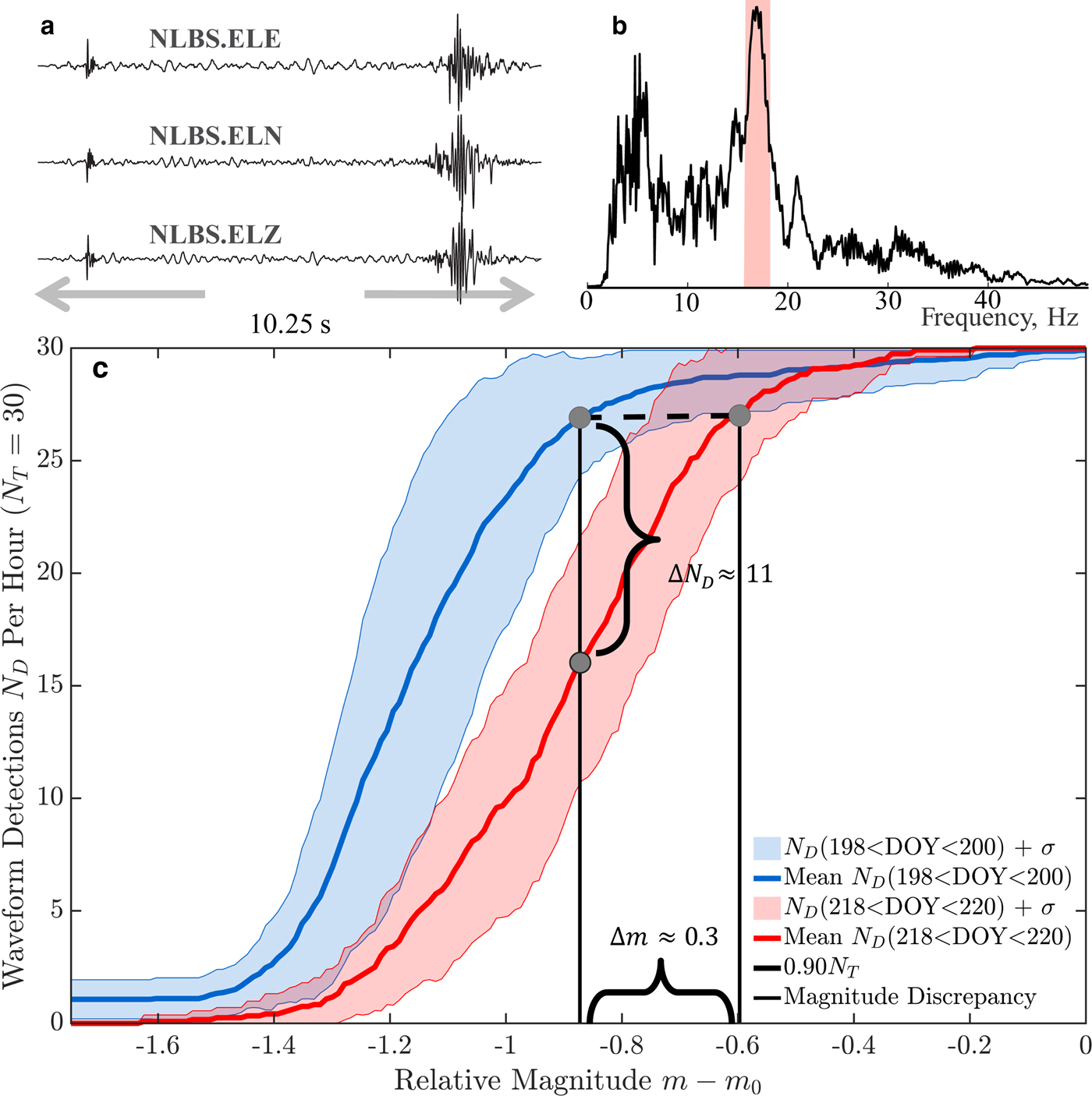
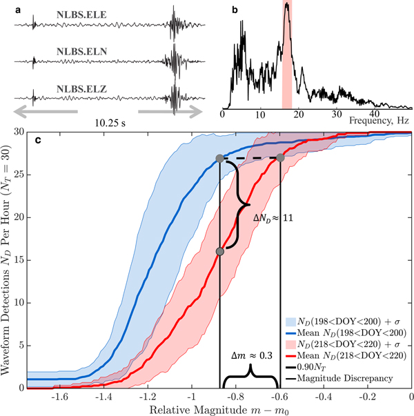
First, we selected a three-channel template waveform w(t) that recorded significant spectral energy at ξ ~17  Hz on geophone NLBS to match the resonance pole frequency recorded between DOY 218 and 220. Our selection process computed short-time vertical-channel spectrograms from pre-resonance data, and measured the ratio of the energy in these spectrograms over 15.75–18.25 Hz, to that over 7.5–25 Hz. We then selected the time bin and associated waveform that maximized this ratio (~ 55%), and labeled the unknown magnitude of the source that produced this waveform as m ₀ (unitless). Second, we amplitude-scaled w(t) by A to mimic waveform amplitudes produced by a hypothetical source of magnitude m (amplitude $A=10^{m-m_{0}}$). The base-10 logarithmic difference between this scaled and original waveform amplitude therefore measures the relative source magnitude m − m ₀. Third, we infused these waveforms into noisy geophone data recorded between DOY 198 and 200 and between DOY 218 and 220, and then processed these data with a constant false alarm probability (Pr_FA = 10⁻¹⁰) correlator. We then counted the number of resultant correlation detections N _D over our relative magnitude grid m − m ₀. We weighted these curves by uncertainty, normalized our counts by the true number of infused waveforms N _T (= 30 per hour), and averaged these weighted, normalized counts into bins. The locus of points $(m-m_0,{\mkern 1mu} \displaystyle{{N_{\rm D}} \over {N_{\rm T}}})$ approximate our correlator's detection probability Pr_D versus relative source magnitude. The section titled Correlation Detectors of our Electronic Supplement details this process.

Our resultant performance curves predict higher detection rates for repeating icequakes that match w(t) in shape and that precede resonance, when compared to resonance-coincident performance curves. Specifically, our correlator detects (1) repeating icequake waveforms that are contaminated by noise and triggered by m − m ₀ ≈− 0.9 magnitude sources with the same Pr_D = 0.9 probability that it detects (2) icequake waveforms contaminated by noise plus narrowband interference that are triggered by m − m ₀ ≈− 0.6 magnitude sources (Fig. 3). This means that waveforms like A w(t) that are triggered by a seismic source of magnitude m − m ₀ ≈− 0.9 are less detectable if they are triggered during times when a geophone also records a narrowband source: specifically, only ~ 53% of such waveforms, on average, are detectable with Pr_D = 0.9 detection probability when the false alarm probability is Pr_FA = 10⁻¹⁰. The resonance signal therefore reduces apparent icequake emission rates by about 40%. We emphasize that the particular values of these detection rates are conditional on the noise environment, and the time-bandwidth product of both the template and target data.

Fig. 3.

(a) A three-channel correlator template w(t) recorded by geophone NLBS on DOY 173, 2011. (b) The normalized, channel-averaged power spectral of w(t). The highlighted band $15.75 \le {\rm }{\rm \xi } \le 18.25$ Hz marks spectral overlap with geophone pole resonance, recorded DOY 218–220. (c) Performance curves for the correlator during pre- and resonance-coincident times. Solid curves measure the number of data-infused, amplitude-scaled waveforms that the correlator detected, versus magnitude of the target source, relative to that of the source that produced w(t). Shaded regions measure performance uncertainty as a standard deviation (± σ) from the mean curve. The horizontal brace measures correlator performance loss (discrepancy) as the difference between (1) the magnitude at which the correlator detects resonance-contaminated target waveforms with Pr_D = 0.9 (N _D = 0.9 N _T), and (2) the magnitude at which the correlator detects target waveforms with that same probability, when it processes resonance-free data. The vertical brace marks the reduced number of detections from a m − m ₀ = − 0.9 magnitude source.

DISCUSSION AND CONCLUSIONS

We present three conclusions from our analysis of geophone data collected from the ablation zone of the Western GrIS.

First, resonance of geophone installation structures during melt-out can excite narrowband signals that mimic some general features of moulin tremor in regions where such tremor is expected. Therefore, records collected from geophones that are mounted on resonance-susceptible structures and installed near sources of hydraulic signal can record both glaciogenic and artificial, narrowband sources. Published (Podolskiy and Walter, Reference Podolskiy and Walter2016) and unpublished installation concepts document similar deployment strategies (see Installation Methods in our Electronic supplement). As absorption of shortwave radiation often drives ablation of surface glacial ice (van den Broeke and others, Reference van den Broeke, Smeets, Ettema and Munneke2008), we suggest that buried geophone installation schemes exploit a radiation cover over the buried site, like a blanket or tarp. This cover may prevent geophone melt-out and the subsequent resonance as we quantified here.

Second, the resonance of the geophone installation structure during melt-out is a signature that the sensor is decoupled from the ice, and cannot record transient waveform data either inside and outside the resonance band. We estimate that an exposure length ≥ 1.25 m of our installation pole mitigated geophone-to-ice coupling that enabled our sensors to previously record icequakes or earthquakes, prior to the onset of resonance. This post-resonance decoupling hindered our ability to confidently identify any waveform, regardless of their spectral characteristics.

Third, digital waveform detectors that process records of narrowband signals show a reduced capability to detect transient icequake waveforms even when sensors remain coupled to the ice, and when waveforms spectrally overlap with the narrowband signals. Such narrowband signals inhibit detectors regardless of source type (glaciogenic or structural resonance). Our data specifically test correlators that process geophone data contaminated by narrowband signals whose variance exceeds that of ambient background noise by ≥ 100 ×. In this case, a correlator can detect waveforms triggered by a source that is 0.6 magnitude units less than that of the template, with a 0.9 probability. In the absence of this narrowband interference, the same correlator can detect waveforms about 0.3 magnitude units smaller at the same probability. Thus, the presence of narrowband, tremor-like signals quantifiably suppresses the detection of repeatable, transient icequake waveforms. This suppression mimics the intent of radar signal jammers onboard military aircraft that evade tracking systems by radiating sinusoidal signals in the spectral range of the tracking system radar (Milstein, Reference Milstein1988). Analogously, a coincident recording of a tremor-like signal along with a decrease of icequake detections can reflect a loss of detection capability, rather than a decrease of icequakes during tremor-like episodes.

Last, we do not challenge the conclusions of Röösli and others (Reference Röösli, Walter, Ampuero and Kissling2016) that their recorded signal shows resonance within a partially water-filled moulin. Our data do show, however, that geophone records can capture sources of installation-related resonance from regions on the GrIS that host true, glaciogenic resonance (like seismic moulin tremor). Cryoseismologists must quantify the temporal and spectral limits of their receiver installation systems under melt season forcing, prior to concluding that these signals have glaciogenic sources.

DATA

IRIS archives Greenland Supraglacial Lakes project seismic data that were recorded year 2011 under network code Y6 here: http://ds.iris.edu/SeismiQuery/. Data processing implemented MATLAB CORAL functions authored by Ken Creager and Joshua D Carmichael. Utrecht University makes RACMO resources available here: https://www.projects.science.uu.nl/iceclimate/models/greenland.php.