


1. Introduction
Solutes spread and mix in deformable porous media in a variety of geomechanical, industrial and biological contexts. In general, the transport of solutes in porous media is driven by molecular diffusion and by internal fluid flow. In soft porous media, the latter is strongly coupled to external mechanical loads through rearrangement of the pore structure (e.g. Mow et al. Reference Mow, Kuei, Lai and Armstrong1980; Lai, Hou & Mow Reference Lai, Hou and Mow1991; Preziosi, Joseph & Beavers Reference Preziosi, Joseph and Beavers1996; Li, Borja & Regueiro Reference Li, Borja and Regueiro2004; Franceschini et al. Reference Franceschini, Bigoni, Regitnig and Holzapfel2006; Ehlers, Karajan & Markert Reference Ehlers, Karajan and Markert2009; Moeendarbary et al. Reference Moeendarbary, Valon, Fritzsche, Harris, Moulding, Thrasher, Stride, Mahadevan and Charras2013; Vuong, Yoshihara & Wall Reference Vuong, Yoshihara and Wall2015; Borja & Choo Reference Borja and Choo2016). In many cases, these loads are periodic; for example, compression due to surface loading can induce the spreading of contaminants in soils, exacerbating environmental harm and hindering remediation, while physiological loads can drive nutrient transport and waste removal in biological tissues, thus potentially playing an important role in cell growth and survival. In a companion study (Fiori, Pramanik & MacMinn Reference Fiori, Pramanik and MacMinn2023), we examined the poromechanics of periodic loading over a wide range of loading periods and amplitudes. Here, we examine the implications of those results for solute transport.
At the continuum (Darcy) scale, which is the framework of this study, solute transport occurs through three fundamental mechanisms: advection, diffusion and hydrodynamic dispersion (Saffman Reference Saffman1959; Scheidegger Reference Scheidegger1961; Whitaker Reference Whitaker1967; Bear Reference Bear1972; Brenner & Edwards Reference Brenner and Edwards1993; Gelhar Reference Gelhar1993; Whitaker Reference Whitaker1998; Dentz et al. Reference Dentz, Le Borgne, Englert and Bijeljic2011). Diffusion in a porous medium is weaker than in a bulk fluid because of the tortuosity of the pore space (Bear Reference Bear1972; Ghanbarian et al. Reference Ghanbarian, Hunt, Ewing and Sahimi2013; Tartakovsky & Dentz Reference Tartakovsky and Dentz2019). Both advection and dispersion are driven by fluid flow. Advection is driven by the mean interstitial fluid velocity. Dispersion results from the pore-scale deviations from this Darcy-scale mean. In particular, dispersion is driven by two phenomena: (i) analogously to classical Taylor dispersion in a tube (Taylor Reference Taylor1953; Brenner & Stewartson Reference Brenner and Stewartson1980; Marbach & Alim Reference Marbach and Alim2019), pore-scale velocity gradients smear solute profiles along the flow direction, inducing longitudinal spreading, and (ii) the morphology of the pore structure introduces chaotic variability in the fluid streamlines (de Anna et al. Reference de Anna, Le Borgne, Dentz, Tartakovsky, Bolster and Davy2013; Datta et al. Reference Datta, Chiang, Ramakrishnan and Weitz2013; Lester, Metcalfe & Trefry Reference Lester, Metcalfe and Trefry2013, Reference Lester, Metcalfe and Trefry2016a ,Reference Lester, Trefry and Metcalfeb; Kree & Villermaux Reference Kree and Villermaux2017; Gouze et al. Reference Gouze, Puyguiraud, Porcher and Dentz2021; Dentz, Hidalgo & Lester Reference Dentz, Hidalgo and Lester2023; Souzy et al. Reference Souzy, Lhuissier, Méheust, Le Borgne and Metzger2020), thus inducing both longitudinal and transverse spreading (Scheidegger Reference Scheidegger1961; Gelhar & Axness Reference Gelhar and Axness1983; Gelhar, Welty & Rehfeldt Reference Gelhar, Welty and Rehfeldt1992; Delgado Reference Delgado2007). In soft porous media, therefore, deformation can enhance the transport of solutes directly by driving fluid flow, thus leading to advection and dispersion, and indirectly by distorting the pore space, and thus modifying both dispersion and diffusion.
Solute transport in deformable porous media has been studied in several different contexts. The impact of monotonic soil consolidation on transport has been studied extensively for its relevance to the management of landfills and other contaminated sediments, such as dredging or mining waste (e.g. Smith Reference Smith2000; Peters & Smith Reference Peters and Smith2002; Alshawabkeh & Rahbar Reference Alshawabkeh and Rahbar2006; Fox Reference Fox2007a ,Reference Fox b ; Arega & Hayter Reference Arega and Hayter2008; Lewis, Pivonka & Smith Reference Lewis, Pivonka and Smith2009; Zhang et al. Reference Gelhar, Welty and Rehfeldt2012, Reference Ghanbarian, Hunt, Ewing and Sahimi2013; Xie et al. Reference Xie, Yan, Feng, Wang and Chen2016; Pu, Fox & Shackelford Reference Pu, Fox and Shackelford2018; Bonazzi, Jha & de Barros Reference Bonazzi, Jha and de Barros2021). In that context, it is well known that consolidation enhances solute transport. Deformation has also been shown to increase mixing and reduce breakthrough time in the context of miscible viscous fingering (Tran & Jha Reference Tran and Jha2020). The key feature introduced by periodic loading is the continuously fluctuating fluid flow, which can irreversibly modify diffusion and dispersion even when the macroscopic advective component is perfectly reversible. The role of periodic flow in enhancing solute transport and mixing has been studied in rigid and compressible one-dimensional (1-D) pore networks (Goldsztein & Santamarina Reference Goldsztein and Santamarina2004; Claria, Goldsztein & Santamarina Reference Claria, Goldsztein and Santamarina2012). In a poroelastic material, solute transport due to small periodic deformations has been explored across a range of parameters, including compressibility and forcing frequency, for semi-infinite homogeneous systems (Pool, Dentz & Post Reference Pool, Dentz and Post2016), finite homogeneous systems (Bonazzi et al. Reference Bonazzi, Jha and de Barros2021) and finite heterogeneous systems (Trefry et al. Reference Trefry, Lester, Metcalfe and Wu2019; Wu et al. Reference Wu, Lester, Trefry and Metcalfe2020). The latter two studies focus in particular on the combined role of poroelasticity, heterogeneity and transient forcing in generating chaotic advection.
Periodic loading is also known to enhance the transport of nutrients in biological tissues (Ferguson, Ito & Pyrak-Nolte Reference Ferguson, Ito and Pyrak-Nolte2004; Gardiner et al. Reference Gardiner, Smith, Pivonka, Grodzinsky, Frank and Zhang2007; Zhang & Szeri Reference Zhang and Szeri2008; Schmidt et al. Reference Schmidt, Shirazi-Adl, Galbusera and Wilke2010; Zhang Reference Zhang2011; Witt et al. Reference Witt, Duda, Bergmann and Petersen2014; DiDomenico et al. Reference DiDomenico, Goodearl, Yarilina, Sun, Mitra, Sterman and Bonassar2017). Similarly, periodic deformations are used to enhance the infiltration of solutes into hydrogels (Albro et al. Reference Albro, Chahine, Li, Yeager, Hung and Ateshian2008; Vaughan et al. Reference Vaughan, Galie, Stegemann and Grotberg2013) and other scaffolds for tissue engineering (Mauck, Hung & Ateshian Reference Mauck, Hung and Ateshian2003; Cortez, Completo & Alves Reference Cortez, Completo and Alves2016; Fan et al. Reference Fan, Pei, Lucas Lu and Wang2016; Kumar, Dey & Sekhar Reference Kumar, Dey and Raja Sekhar2018), where the correlation between loading parameters, nutrient transport and cell survival is of particular interest. Increasing the loading amplitude and/or decreasing the loading period induces a transition from diffusion-dominated to advection-dominated regimes (Urciuolo, Imparato & Netti Reference Urciuolo, Imparato and Netti2008) and amplifies the role of hydrodynamic dispersion (Sengers, Oomens & Baaijens Reference Sengers, Oomens and Baaijens2004). Decreasing the loading period also leads to localisation of flow and deformation near permeable boundaries, resulting in larger velocities near the surface that promote external solute infiltration (Gardiner et al. Reference Gardiner, Smith, Pivonka, Grodzinsky, Frank and Zhang2007; Urciuolo et al. Reference Urciuolo, Imparato and Netti2008; Vaughan et al. Reference Vaughan, Galie, Stegemann and Grotberg2013; DiDomenico et al. Reference DiDomenico, Goodearl, Yarilina, Sun, Mitra, Sterman and Bonassar2017).
In general, despite the established role of hydrodynamic dispersion in driving the transport of solutes in porous media, dispersion is rarely included in biomechanical models (with the notable exception of Sengers et al. Reference Sengers, Oomens and Baaijens2004). One context where dispersion is widely agreed to be important is in brain microcirculation (Kelley & Thomas Reference Kelley and Thomas2023). In the vascular network within the brain, dispersion results from the shear-induced radial concentration gradients in single vessels (e.g. Marbach and Alim Reference Marbach and Alim2019; Sharp et al. Reference Sharp, Carare and Bryn2019; Berg et al. Reference Berg, Davit, Quintard and Lorthois2020; Troyetsky et al. Reference Troyetsky, Tithof, Thomas and Kelley2021; Bojarskaite et al. Reference Bojarskaite, Vallet, Bjørnstad, Gullestad Binder, Cunen, Heuser, Kuchta, Mardal and Enger2023) and the progressive bifurcation of vessels into smaller branches that can be modelled at the continuum scale as a porous material (e.g. Zimmerman and Tartakovsky Reference Zimmerman and Tartakovsky2020; Goirand, Borgne & Lorthois Reference Goirand, Borgne and Lorthois2021).
Dispersion is typically neglected in the context of tissues and gels for two main reasons. First, fluid flow is often assumed to be slow, implying that transport is dominated by diffusion. In other words, the Péclet number
 $\mathrm {Pe}=VL/\mathcal {D}_m$
is assumed to be small, where
$\mathrm {Pe}=VL/\mathcal {D}_m$
is assumed to be small, where
 $V$
is the characteristic fluid velocity,
$V$
is the characteristic fluid velocity,
 $L$
the characteristic streamwise length scale and
$L$
the characteristic streamwise length scale and
 $\mathcal {D}_m$
the molecular diffusivity. However, it is straightforward to show that
$\mathcal {D}_m$
the molecular diffusivity. However, it is straightforward to show that
 $\mathrm {Pe}$
can be order 1 or larger in a tissue or gel subject to fast (
$\mathrm {Pe}$
can be order 1 or larger in a tissue or gel subject to fast (
 $0.1{-}1$
Hz) and large (
$0.1{-}1$
Hz) and large (
 $10{-}20\,\%$
) deformations (see table 2), suggesting that dispersion may be important or even dominant in some scenarios (Delgado Reference Delgado2007). Indeed, many studies highlight a transition from diffusion-dominated to advection-dominated transport without acknowledging the potential role of dispersion (Gardiner et al. Reference Gardiner, Smith, Pivonka, Grodzinsky, Frank and Zhang2007; Urciuolo et al. Reference Urciuolo, Imparato and Netti2008; Vaughan et al. Reference Vaughan, Galie, Stegemann and Grotberg2013; DiDomenico et al. Reference DiDomenico, Goodearl, Yarilina, Sun, Mitra, Sterman and Bonassar2017). With an analogous argument, Davit et al. (Reference Davit, Byrne, Osborne, Pitt-Francis, Gavaghan and Quintard2013) illustrated the importance of including dispersion in models for solute transport in biofilms. The second typical reason for neglecting dispersion in tissues and gels is the assumption that the longitudinal and transverse dispersivities themselves are negligible. This expectation is a result of physical insight derived from transport in granular materials, where the dispersivity is typically taken to be proportional to the pore size (Saffman Reference Saffman1959; Oswald & Kinzelbach Reference Oswald and Kinzelbach2004; Kree & Villermaux Reference Kree and Villermaux2017; Liang et al. Reference Liang, Wen, Hesse and DiCarlo2018). Indeed, the typical pore size is
$10{-}20\,\%$
) deformations (see table 2), suggesting that dispersion may be important or even dominant in some scenarios (Delgado Reference Delgado2007). Indeed, many studies highlight a transition from diffusion-dominated to advection-dominated transport without acknowledging the potential role of dispersion (Gardiner et al. Reference Gardiner, Smith, Pivonka, Grodzinsky, Frank and Zhang2007; Urciuolo et al. Reference Urciuolo, Imparato and Netti2008; Vaughan et al. Reference Vaughan, Galie, Stegemann and Grotberg2013; DiDomenico et al. Reference DiDomenico, Goodearl, Yarilina, Sun, Mitra, Sterman and Bonassar2017). With an analogous argument, Davit et al. (Reference Davit, Byrne, Osborne, Pitt-Francis, Gavaghan and Quintard2013) illustrated the importance of including dispersion in models for solute transport in biofilms. The second typical reason for neglecting dispersion in tissues and gels is the assumption that the longitudinal and transverse dispersivities themselves are negligible. This expectation is a result of physical insight derived from transport in granular materials, where the dispersivity is typically taken to be proportional to the pore size (Saffman Reference Saffman1959; Oswald & Kinzelbach Reference Oswald and Kinzelbach2004; Kree & Villermaux Reference Kree and Villermaux2017; Liang et al. Reference Liang, Wen, Hesse and DiCarlo2018). Indeed, the typical pore size is
 $\sim 10$
nm in polymeric gels and in the extra-cellular matrix of tissues (e.g. around 6 nm in cartilage, Mow, Holmes & Lai (Reference Mow, Holmes and Lai1984)) and can therefore be similar to (or smaller than) the size of large solute molecules (Maroudas Reference Maroudas1970; DiDomenico, Lintz & Bonassar Reference DiDomenico, Lintz and Bonassar2018), causing solid–solute friction (Yao & Gu Reference Yao and Gu2007; Ateshian et al. Reference Ateshian, Albro, Maas and Weiss2011). However, tissues and scaffolds are heterogeneous and multiscale materials; the presence of other components, such as collagen fibres, results in a ‘mesoscale’ of larger pores (e.g. 100–150 nm in cartilage, Maroudas (Reference Maroudas1975); Levick (Reference Levick1987); Federico & Herzog (Reference Federico and Herzog2008)), where even larger solute molecules can pass (DiDomenico et al. Reference Lester, Dentz and Le Borgne2017, Reference Pool, Dentz and Post2018) and where dispersion is likely to play a much larger role. The same is true for double-porosity scaffolds and gels, where additional channels and/or macroscopic pores are included to enhance fluid flow throughout the scaffold depth (Buijs, Ritman & Dragomir-Daescu Reference Buijs, Ritman and Dragomir-Daescu2010; Mesallati et al. Reference Mesallati, Buckley, Nagel and Kelly2013; Lee et al. Reference Lee, Rich, Baek, Lee and Kong2015). As a further counter-argument, we hypothesise that, even in pores that are small compared with the solute molecules, the irrelevance of pore-scale velocity gradients does not exclude velocity variations and streamline alterations in the overall network, which could cause longitudinal and transverse dispersion. This hypothesis is consistent with the quantification of tortuosity in several soft tissues (Maroudas Reference Maroudas1970; Hrabe, Hrabĕtová & Segeth Reference Hrabe, Hrabĕtová and Segeth; Zhang and Szeri Reference Zhang and Szeri2005).
$\sim 10$
nm in polymeric gels and in the extra-cellular matrix of tissues (e.g. around 6 nm in cartilage, Mow, Holmes & Lai (Reference Mow, Holmes and Lai1984)) and can therefore be similar to (or smaller than) the size of large solute molecules (Maroudas Reference Maroudas1970; DiDomenico, Lintz & Bonassar Reference DiDomenico, Lintz and Bonassar2018), causing solid–solute friction (Yao & Gu Reference Yao and Gu2007; Ateshian et al. Reference Ateshian, Albro, Maas and Weiss2011). However, tissues and scaffolds are heterogeneous and multiscale materials; the presence of other components, such as collagen fibres, results in a ‘mesoscale’ of larger pores (e.g. 100–150 nm in cartilage, Maroudas (Reference Maroudas1975); Levick (Reference Levick1987); Federico & Herzog (Reference Federico and Herzog2008)), where even larger solute molecules can pass (DiDomenico et al. Reference Lester, Dentz and Le Borgne2017, Reference Pool, Dentz and Post2018) and where dispersion is likely to play a much larger role. The same is true for double-porosity scaffolds and gels, where additional channels and/or macroscopic pores are included to enhance fluid flow throughout the scaffold depth (Buijs, Ritman & Dragomir-Daescu Reference Buijs, Ritman and Dragomir-Daescu2010; Mesallati et al. Reference Mesallati, Buckley, Nagel and Kelly2013; Lee et al. Reference Lee, Rich, Baek, Lee and Kong2015). As a further counter-argument, we hypothesise that, even in pores that are small compared with the solute molecules, the irrelevance of pore-scale velocity gradients does not exclude velocity variations and streamline alterations in the overall network, which could cause longitudinal and transverse dispersion. This hypothesis is consistent with the quantification of tortuosity in several soft tissues (Maroudas Reference Maroudas1970; Hrabe, Hrabĕtová & Segeth Reference Hrabe, Hrabĕtová and Segeth; Zhang and Szeri Reference Zhang and Szeri2005).
Thus, the impact of periodic loading on solute transport in soft porous media has been addressed with various approaches and assumptions across a variety of specific applications in soils, tissues, hydrogels and scaffolds. However, no single study has yet provided a comprehensive understanding across a wide range of loading frequencies and amplitudes. Moreover, the impact of hydrodynamic dispersion remains relatively unexplored and therefore poorly understood, particularly in the context of biological and biomedical applications. Here, we study the transport and mixing of solutes due to arbitrarily large, periodic deformations of a soft porous material. For the flow and deformation, we adopt a 1-D, large-deformation poroelasticity model that includes rigorous nonlinear kinematics, deformation-dependent permeability and Hencky elasticity for the solid skeleton. In a companion study, we used this model to explore the poromechanics of large-amplitude periodic loading (Fiori et al. Reference Fiori, Pramanik and MacMinn2023). Here, we additionally consider solute transport due to advection, diffusion and dispersion. We first study the separate roles of advection, diffusion and dispersion during one loading cycle. We then consider the impact of the transport and loading parameters on transport and mixing over longer time periods and/or larger numbers of loading cycles. We report the impact of a wide range of loading amplitudes and periods on each transport mechanism and observe how transport depends on the poromechanical response through its impact on local fluid flow. When dispersion is negligible, we show that diffusion is insensitive to loading period but slightly suppressed by increased loading amplitude. With dispersion, larger amplitudes always boost solute spreading; however, progressively shorter periods impact transport and mixing in more complex ways: fast loading promotes spreading by inducing large fluid velocities, but very fast loading hinders spreading by progressively localising the flow and deformation. We show that the competition between these two effects results in maximum solute transport and mixing for intermediate loading periods.
2. Theoretical model
Our model combines large-deformation poroelasticity with solute transport. The coupling between periodic deformations and solute movement occurs primarily via the fluid flow, which is caused by the former and responsible for the latter.
2.1. Model problem
We consider a 1-D sample of soft porous material of relaxed length
 $L$
and relaxed porosity (fluid fraction)
$L$
and relaxed porosity (fluid fraction)
 $\phi _{f,0}$
. The left boundary of the material (at
$\phi _{f,0}$
. The left boundary of the material (at
 $x=a(t))$
is moving and permeable, whereas the right boundary (at
$x=a(t))$
is moving and permeable, whereas the right boundary (at
 $x=L$
) is fixed and impermeable. The position of the left boundary,
$x=L$
) is fixed and impermeable. The position of the left boundary,
 $a(t)$
, is imposed to be
$a(t)$
, is imposed to be
 \begin{equation} a(t)= \frac {A}{2} \left [1-\cos \left (\frac {2\pi t}{T}\right )\right ], \end{equation}
where
 $A$
and
$A$
and
 $T$
are the amplitude and period of loading, respectively. We consider imposed deformations ranging from small to large macroscopic strains (
$T$
are the amplitude and period of loading, respectively. We consider imposed deformations ranging from small to large macroscopic strains (
 $-0.4\,\%$
to
$-0.4\,\%$
to
 $-20\,\%$
or
$-20\,\%$
or
 $0.004\leq {}A/L\leq {}0.2$
). We take the fluid and solid to be individually incompressible, such that changes in bulk volume correspond directly to the movement of fluid into and out of the pore space. We presented and analysed the poromechanics of this scenario in detail in a companion study (Fiori et al. Reference Fiori, Pramanik and MacMinn2023). We now introduce a strip of passive solute of initial width
$0.004\leq {}A/L\leq {}0.2$
). We take the fluid and solid to be individually incompressible, such that changes in bulk volume correspond directly to the movement of fluid into and out of the pore space. We presented and analysed the poromechanics of this scenario in detail in a companion study (Fiori et al. Reference Fiori, Pramanik and MacMinn2023). We now introduce a strip of passive solute of initial width
 $l$
located at the right boundary and we study the impact of this periodic, displacement-driven deformation on the evolution of the solute distribution (figure 1).
$l$
located at the right boundary and we study the impact of this periodic, displacement-driven deformation on the evolution of the solute distribution (figure 1).
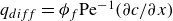
We consider a 1-D sample of soft porous material of relaxed length
 $L$
, subject to a periodic, displacement-driven loading at its left boundary (white arrows). The left boundary is permeable, thus allowing fluid flow in or out (pale blue squiggles) to accommodate the loading. The right boundary is fixed and impermeable. The solute is initially localised against the right boundary in a strip of width
$L$
, subject to a periodic, displacement-driven loading at its left boundary (white arrows). The left boundary is permeable, thus allowing fluid flow in or out (pale blue squiggles) to accommodate the loading. The right boundary is fixed and impermeable. The solute is initially localised against the right boundary in a strip of width
 $l$
(dark blue).
$l$
(dark blue).

2.2. Kinematics
We consider an Eulerian reference frame, in which the solid displacement is
 $\mathbf {u}_{\mathbf {s}}=\mathbf {x}-\mathbf {X}(\mathbf {x},t)$
, with
$\mathbf {u}_{\mathbf {s}}=\mathbf {x}-\mathbf {X}(\mathbf {x},t)$
, with
 $\mathbf {X}(\mathbf {x},t)$
the reference position of the solid material point that at time
$\mathbf {X}(\mathbf {x},t)$
the reference position of the solid material point that at time
 $t$
occupies position
$t$
occupies position
 $\mathbf {x}$
. We choose our reference configuration to be the relaxed configuration, such that
$\mathbf {x}$
. We choose our reference configuration to be the relaxed configuration, such that
 $\mathbf {X}(\mathbf {x},0)=\mathbf {x}$
and
$\mathbf {X}(\mathbf {x},0)=\mathbf {x}$
and
 $\mathbf {u}_{\mathbf {s}}(\mathbf {x},0)=0$
. The true volume fractions of fluid and solid are
$\mathbf {u}_{\mathbf {s}}(\mathbf {x},0)=0$
. The true volume fractions of fluid and solid are
 $\phi _f$
and
$\phi _f$
and
 $\phi _{s}$
, respectively, where
$\phi _{s}$
, respectively, where
 $\phi _{f}+\phi _{s}=1$
. In this uniaxial setting, the solid displacement and the solid and fluid velocities are one-dimensional and given by
$\phi _{f}+\phi _{s}=1$
. In this uniaxial setting, the solid displacement and the solid and fluid velocities are one-dimensional and given by
 \begin{equation} \mathbf{u}_{\mathbf{s}}=u_{s}(x,t) {\hat {\mathbf{e}}_{\mathbf {x}}}, \; \mathbf {v}_{\mathbf {s}} = v_{s}(x,t) {\hat {\mathbf{e}}_{\mathbf {x}}}, \; \mathbf {v}_{\mathbf {f}} = v_{f}(x,t) {\hat{\mathbf{e}}_{\mathbf {x}}}, \end{equation}
where
 $\mathbf {v}_{\mathbf {f}}$
and
$\mathbf {v}_{\mathbf {f}}$
and
 $\mathbf {v}_{\mathbf {s}}$
are the fluid and solid velocities, respectively,
$\mathbf {v}_{\mathbf {s}}$
are the fluid and solid velocities, respectively,
 $u_s$
,
$u_s$
,
 $v_s$
and
$v_s$
and
 $v_f$
are the
$v_f$
are the
 $x$
-components of these fields and
$x$
-components of these fields and
 ${\hat {\mathbf e}_{\mathbf {x}}}$
is the unit vector in the
${\hat {\mathbf e}_{\mathbf {x}}}$
is the unit vector in the
 $x$
-direction. The local current volume per unit reference volume is measured by the Jacobian determinant, which in this uniaxial setting is given by
$x$
-direction. The local current volume per unit reference volume is measured by the Jacobian determinant, which in this uniaxial setting is given by
 $J= (1-\partial {u_s}/\partial {x})^{-1}$
. For incompressible constituents and uniform initial porosity
$J= (1-\partial {u_s}/\partial {x})^{-1}$
. For incompressible constituents and uniform initial porosity
 $\phi _{f,0}$
, the local change in volume relates to the change in porosity as
$\phi _{f,0}$
, the local change in volume relates to the change in porosity as
 \begin{equation} J(x,t) = \frac {1-\phi _{f,0}}{1-\phi _f} \quad \to \quad \frac {\partial {u_s}}{\partial {x}} =\frac {\phi _f-\phi _{f,0}}{1-\phi _{f,0}}. \end{equation}
Continuity can be written
 \begin{equation} \frac {\partial {\phi _f}}{\partial {t}} +\frac {\partial }{\partial {x}}(\phi _f v_f) = 0 \quad \mathrm {and}\quad \frac {\partial {\phi _f}}{\partial {t}} -\frac {\partial }{\partial {x}}{[(1-\phi _f)v_s]} = 0, \end{equation}
which together imply that the total flux
 $q=\phi _fv_f+(1-\phi _f)v_s$
is uniform in space,
$q=\phi _fv_f+(1-\phi _f)v_s$
is uniform in space,
 $\partial {q}/\partial {x}=0$
.
$\partial {q}/\partial {x}=0$
.
2.3. Fluid flow
We assume that the fluid flows relative to the solid according to Darcy’s law
 \begin{equation} \phi _ f (v_{f}-v_{s}) = - \frac {k(\phi _f)}{\mu }\frac {\partial p}{\partial x}, \end{equation}
where
 $k(\phi _f)$
is the permeability of the solid skeleton,
$k(\phi _f)$
is the permeability of the solid skeleton,
 $\mu$
is the dynamic viscosity of the fluid and
$\mu$
is the dynamic viscosity of the fluid and
 $p$
is the fluid (pore) pressure, and where we have neglected gravity. As in Fiori et al. (Reference Fiori, Pramanik and MacMinn2023), we take the permeability to be deformation-dependent according to a normalised Kozeny–Carman relation,
$p$
is the fluid (pore) pressure, and where we have neglected gravity. As in Fiori et al. (Reference Fiori, Pramanik and MacMinn2023), we take the permeability to be deformation-dependent according to a normalised Kozeny–Carman relation,
 $k(\phi _{f}) = k_0 ({(1-\phi _{f,0})^2}/{\phi _{f,0}^3}) ({\phi _{f}^3}/{(1-\phi _{f})^2})$
, where
$k(\phi _{f}) = k_0 ({(1-\phi _{f,0})^2}/{\phi _{f,0}^3}) ({\phi _{f}^3}/{(1-\phi _{f})^2})$
, where
 $k_0\equiv {}k(\phi _{f,0})$
is the permeability of the initial state. We discuss this choice in detail in Fiori et al. (Reference Fiori, Pramanik and MacMinn2023).
$k_0\equiv {}k(\phi _{f,0})$
is the permeability of the initial state. We discuss this choice in detail in Fiori et al. (Reference Fiori, Pramanik and MacMinn2023).
Combining (2.4) and (2.5), we arrive at the nonlinear flow equations
 \begin{equation} \frac {\partial {\phi _f}}{\partial {t}} +\frac {\partial }{\partial {x}}\bigg [{\phi _f q}-(1-\phi _f) \frac {k(\phi _f)}{\mu }\frac {\partial {p}}{\partial {x}}\bigg ]=0 \quad \mathrm {and}\quad \frac {\partial {q}}{\partial {x}}=0, \end{equation}
where the total flux
 $q$
is again
$q$
is again
 \begin{equation} q\equiv \phi _f v_f + (1-\phi _f)v_s, \end{equation}
and the fluid and solid velocities are given by
 \begin{equation} v_f=q-\frac {(1-\phi _f)}{\phi _f}\frac {k(\phi _f)}{\mu }\frac {\partial p}{\partial x} \quad \mathrm {and}\quad v_s=q+\frac {k(\phi _f)}{\mu }\frac {\partial p}{\partial x}. \end{equation}
Note that the fluid flux is
 \begin{equation} q_f=\phi _f v_f. \end{equation}
2.4. Mechanical equilibrium and elasticity law
Neglecting inertia, gravity and other body forces, mechanical equilibrium can be expressed as
 ${\boldsymbol {\nabla }\cdot {\boldsymbol {\sigma }}}= {\boldsymbol {\nabla }\cdot {\boldsymbol {\sigma '}}}-\boldsymbol {\nabla } p= 0$
, where
${\boldsymbol {\nabla }\cdot {\boldsymbol {\sigma }}}= {\boldsymbol {\nabla }\cdot {\boldsymbol {\sigma '}}}-\boldsymbol {\nabla } p= 0$
, where
 $\boldsymbol {\sigma }$
is the true Cauchy total stress, decomposed into contributions from the fluid pressure
$\boldsymbol {\sigma }$
is the true Cauchy total stress, decomposed into contributions from the fluid pressure
 $p$
and from Terzaghi’s effective stress
$p$
and from Terzaghi’s effective stress
 $\boldsymbol {\sigma '}$
. In one dimension, mechanical equilibrium reads
$\boldsymbol {\sigma '}$
. In one dimension, mechanical equilibrium reads
 \begin{equation} \frac {\partial \sigma '}{\partial x}=\frac {\partial p}{\partial x}, \end{equation}
where
 $\sigma ^\prime$
is the
$\sigma ^\prime$
is the
 $xx$
component of
$xx$
component of
 $\boldsymbol {\sigma ^\prime}$
.
$\boldsymbol {\sigma ^\prime}$
.
We take the solid skeleton to be elastic, with no viscous or dissipative behaviours. Since any elasticity law can be written in the form
 $\sigma ^\prime =\sigma ^\prime (\phi _f)$
for a uniaxial deformation, this problem can be described by a nonlinear advection-diffusion equation
$\sigma ^\prime =\sigma ^\prime (\phi _f)$
for a uniaxial deformation, this problem can be described by a nonlinear advection-diffusion equation
 \begin{equation} \frac {\partial {\phi _f}}{\partial {t}} +\frac {\partial }{\partial {x}}\bigg [{\phi _f q}-D_f(\phi _f)\frac {\partial {\phi _f}}{\partial {x}}\bigg ]=0 \quad \mathrm {and}\quad \frac {\partial {q}}{\partial {x}}=0, \end{equation}
where the nonlinear composite constitutive function
 \begin{equation} D_f(\phi _f)=(1-\phi _f)\frac {k(\phi _f)}{\mu }\frac {\mathrm {d}\sigma ^\prime }{\mathrm {d}\phi _f} \end{equation}
is the poroelastic diffusivity. Note that a very similar model is used for the solidification of colloidal suspensions in applications such as filtration and sedimentation, for which the poroelastic diffusivity
 $D_f(\phi _f)$
(i.e. the ‘solids diffusivity’) is characterised as a composite material property (e.g. Reference Davis and RusselDavis and Russel 1989; Peppin, Elliott & Worster Reference Peppin, Elliott and Worster2006; Style & Peppin Reference Style and Peppin2011; Bouchaudy and Salmon Reference Bouchaudy and Salmon2019; Worster, Peppin & Wettlaufer Reference Worster, Peppin and Wettlaufer2021).
$D_f(\phi _f)$
(i.e. the ‘solids diffusivity’) is characterised as a composite material property (e.g. Reference Davis and RusselDavis and Russel 1989; Peppin, Elliott & Worster Reference Peppin, Elliott and Worster2006; Style & Peppin Reference Style and Peppin2011; Bouchaudy and Salmon Reference Bouchaudy and Salmon2019; Worster, Peppin & Wettlaufer Reference Worster, Peppin and Wettlaufer2021).
We use Hencky hyperelasticity (Hencky Reference Hencky1931) as a simple, large-deformation model that captures kinematic nonlinearity. For a uniaxial deformation, the relevant component of the effective stress is then
 \begin{equation} \sigma ^\prime = \mathcal {M}\frac {\ln (J)}{J}=\mathcal {M} \left (\frac {1-\phi _f}{1-\phi _{f,0}}\right ) \ln \left (\frac {1-\phi _{f,0}}{1-\phi _f}\right ), \end{equation}
where
 $\mathcal {M}$
is the
$\mathcal {M}$
is the
 $p$
-wave or oedometric modulus (MacMinn, Dufresne & Wettlaufer Reference MacMinn, Dufresne and Wettlaufer2016). Note that, for these constitutive choices of Kozeny–Carman permeability and Hencky elasticity, the permeability at the left boundary can vanish for sufficiently large
$p$
-wave or oedometric modulus (MacMinn, Dufresne & Wettlaufer Reference MacMinn, Dufresne and Wettlaufer2016). Note that, for these constitutive choices of Kozeny–Carman permeability and Hencky elasticity, the permeability at the left boundary can vanish for sufficiently large
 $A$
and/or small
$A$
and/or small
 $T$
, because the poroelastic diffusivity remains finite rather than diverging as
$T$
, because the poroelastic diffusivity remains finite rather than diverging as
 $\phi _f\to 0$
(Hewitt et al. Reference Hewitt, Paterson, Balmforth and Martinez2016). We motivate and discuss our constitutive choices and explore the poroelastic diffusivity in more detail in Fiori et al. (Reference Fiori, Pramanik and MacMinn2023).
$\phi _f\to 0$
(Hewitt et al. Reference Hewitt, Paterson, Balmforth and Martinez2016). We motivate and discuss our constitutive choices and explore the poroelastic diffusivity in more detail in Fiori et al. (Reference Fiori, Pramanik and MacMinn2023).
With appropriate initial conditions, boundary conditions, and the normalised Kozeny–Carman permeability law, equations (2.11), (2.12) and (2.13) comprise a closed model for the evolution of the porosity.
2.5. Solute transport
We now consider the transport of solute. We denote the true local solute concentration in the fluid phase by
 $c$
(amount of solute per unit current fluid volume). We take the solute to be passive and charge neutral, with no chemical or other interaction with the solid or fluid phases, so that neither the fluid properties nor the solid properties depend on
$c$
(amount of solute per unit current fluid volume). We take the solute to be passive and charge neutral, with no chemical or other interaction with the solid or fluid phases, so that neither the fluid properties nor the solid properties depend on
 $c$
. The flow and mechanics above are then independent of the transport problem.
$c$
. The flow and mechanics above are then independent of the transport problem.
In one dimension, it is well known that conservation of mass for a passive solute can be written
 \begin{equation} \frac {\partial }{\partial t} (\phi _f c) +\frac {\partial }{\partial x}\left [{\phi _f c v_f }- \phi _f \mathcal {D} \frac {\partial c}{\partial x}\right ]=0. \end{equation}
The first term in the square brackets is the Darcy-scale solute flux due to advection, which occurs here entirely in response to the deformation. The second term in the square brackets combines molecular diffusion and hydrodynamic dispersion, thus taking the latter to be a Fickian process (e.g. Scheidegger Reference Scheidegger1961). The latter term is multiplied by the porosity
 $\phi _f$
since solute movements only occur in the fluid phase. The coefficient
$\phi _f$
since solute movements only occur in the fluid phase. The coefficient
 $\mathcal {D}$
can be written
$\mathcal {D}$
can be written
 \begin{equation} \mathcal {D} =\mathcal {D}_m+\mathcal {D}_h, \end{equation}
where
 $\mathcal {D}_m$
and
$\mathcal {D}_m$
and
 $\mathcal {D}_h$
are the coefficients of molecular diffusion and hydrodynamic dispersion, respectively. Dispersion, in which pore-scale velocity gradients and the tortuosity of the pore space lead to macroscopic spreading of solute, depends sensitively on flow conditions and the details of the pore structure in ways that are not yet fully understood, even for rigid porous materials (Dentz et al. Reference Urciuolo, Imparato and Netti2018, Reference DiDomenico, Wang and Bonassar2023). The most widely used model for the macroscopic dispersive flux is Fickian, as above, with a velocity-dependent dispersion coefficient given in one dimension by
$\mathcal {D}_h$
are the coefficients of molecular diffusion and hydrodynamic dispersion, respectively. Dispersion, in which pore-scale velocity gradients and the tortuosity of the pore space lead to macroscopic spreading of solute, depends sensitively on flow conditions and the details of the pore structure in ways that are not yet fully understood, even for rigid porous materials (Dentz et al. Reference Urciuolo, Imparato and Netti2018, Reference DiDomenico, Wang and Bonassar2023). The most widely used model for the macroscopic dispersive flux is Fickian, as above, with a velocity-dependent dispersion coefficient given in one dimension by
 \begin{equation} \mathcal {D}_h=\alpha |v_f-v_s|, \end{equation}
where
 $\alpha$
is the longitudinal dispersivity (Scheidegger Reference Scheidegger1961; Brenner & Edwards (Reference Brenner and Edwards1993; Gelhar Reference Gelhar1993; Whitaker Reference Whitaker1998). Note that the dispersive flux is proportional to
$\alpha$
is the longitudinal dispersivity (Scheidegger Reference Scheidegger1961; Brenner & Edwards (Reference Brenner and Edwards1993; Gelhar Reference Gelhar1993; Whitaker Reference Whitaker1998). Note that the dispersive flux is proportional to
 $|v_f-v_s|$
, unlike the advective flux, because dispersion is driven by flow of fluid through the pore structure (i.e.
$|v_f-v_s|$
, unlike the advective flux, because dispersion is driven by flow of fluid through the pore structure (i.e.
 $v_f=v_s\neq 0$
would lead to advection but no dispersion). Note also that, unlike the advective flux, the diffusive and dispersive fluxes are independent of the direction of the fluid flow.
$v_f=v_s\neq 0$
would lead to advection but no dispersion). Note also that, unlike the advective flux, the diffusive and dispersive fluxes are independent of the direction of the fluid flow.
The dispersivity
 $\alpha$
is typically taken to be a constant material property for a given pore structure. In a deforming porous material, and particularly for moderate to large deformations, it is likely that
$\alpha$
is typically taken to be a constant material property for a given pore structure. In a deforming porous material, and particularly for moderate to large deformations, it is likely that
 $\alpha$
should be deformation-dependent to account for the evolving pore structure. For example, particle–particle interactions and rearrangements are known to drive enhanced dispersion in dense suspensions (Souzy et al. Reference Vaughan, Galie, Stegemann and Grotberg2016, Reference Vuong, Yoshihara and Wall2017) and compaction has been shown to have a non-trivial impact on dispersion in bead packs and packed beds (Charlaix, Hulin & Plona Reference Charlaix, Hulin and Plona1987; Östergren & Trägårdh Reference Östergren and Trägårdh2000; Liu et al. Reference Liu, Gong, Xiao and Wang2024). We expect similar but even larger effects in poroelastic materials under large deformations, which may ultimately require novel dispersion models, but these phenomena are beyond the scope of the present study. Here, we take
$\alpha$
should be deformation-dependent to account for the evolving pore structure. For example, particle–particle interactions and rearrangements are known to drive enhanced dispersion in dense suspensions (Souzy et al. Reference Vaughan, Galie, Stegemann and Grotberg2016, Reference Vuong, Yoshihara and Wall2017) and compaction has been shown to have a non-trivial impact on dispersion in bead packs and packed beds (Charlaix, Hulin & Plona Reference Charlaix, Hulin and Plona1987; Östergren & Trägårdh Reference Östergren and Trägårdh2000; Liu et al. Reference Liu, Gong, Xiao and Wang2024). We expect similar but even larger effects in poroelastic materials under large deformations, which may ultimately require novel dispersion models, but these phenomena are beyond the scope of the present study. Here, we take
 $\alpha$
to be a constant for simplicity.
$\alpha$
to be a constant for simplicity.
2.6. Initial and boundary conditions
We next specify initial and boundary conditions for the solid, the fluid and the solute. Recall that the left and right boundaries of the solid are at
 $x=a(t)$
and
$x=a(t)$
and
 $x=L$
, respectively.
$x=L$
, respectively.
2.6.1. Initial conditions
Equation (2.1) implies that
 $a(0)=0$
, and thus that the initial porosity is uniform and equal to the relaxed porosity
$a(0)=0$
, and thus that the initial porosity is uniform and equal to the relaxed porosity
 \begin{equation} \phi _f(x,0)= \phi _{f,0} \textrm { and } u_s(x,0)=0. \end{equation}
We take the solute to be initially localised against the right boundary in a strip of width
 $l$
and concentration
$l$
and concentration
 $c_0$
, such that
$c_0$
, such that
 \begin{equation} c(x,0)=\frac {c_0}{2} \left \{ \tanh {[s(x-L+l)}]+1 \right \}, \end{equation}
where
 $s$
is a steepness parameter.
$s$
is a steepness parameter.
2.6.2. Left boundary
For
 $t\gt 0$
, we apply a displacement-controlled loading at the left boundary according to equation (2.1). We take this moving boundary to be fluid and solute permeable. The associated boundary conditions are
$t\gt 0$
, we apply a displacement-controlled loading at the left boundary according to equation (2.1). We take this moving boundary to be fluid and solute permeable. The associated boundary conditions are
 \begin{equation} u_s(a,t)=a(t), \quad v_s(a,t)=\frac {\mathrm {d}a}{\mathrm {d}t}\quad \mathrm {and}\quad p(a,t)=0. \end{equation}
We take the fluid outside the domain to be ‘clean’, such that
 \begin{equation} c(a,t)=0. \end{equation}
2.6.3. Right boundary
We take the right boundary to be fixed and impermeable, such that
 \begin{equation} u_s(L,t)=v_s(L,t)=v_f(L,t)=0 \quad \mathrm {and} \quad \frac {\partial c}{\partial x}\bigg |_{x=L}=0. \end{equation}
Equation (2.21) and the requirement that
 $q$
be uniform in space imply that there can be no net flow from left to right in our problem,
$q$
be uniform in space imply that there can be no net flow from left to right in our problem,
 $q\equiv 0$
. Equation (2.7) then implies that the fluid and the solid always locally move in opposite directions
$q\equiv 0$
. Equation (2.7) then implies that the fluid and the solid always locally move in opposite directions
 \begin{equation} v_f= -\frac {(1-\phi _f)}{\phi _f} v_s. \end{equation}
2.7. Scaling and summary
As in Fiori et al. (Reference Fiori, Pramanik and MacMinn2023), we apply the following non-dimensionalisation to the poromechanical model:
 \begin{equation} \begin{aligned} \tilde {x}=\frac {x}{L},\; \tilde {u}_s=\frac {u_s}{L},\; \tilde {t}=\frac {t}{T_{pe}},\; \tilde {\sigma }^\prime=\frac {\sigma '}{\mathcal {M}},\; \tilde {p}=\frac {p}{\mathcal {M}},\; \tilde {k}=\frac {k(\phi )}{k_0},\; \tilde {v}_f=\frac {v_f}{L/T_{pe}}, \; \tilde {v}_s=\frac {v_s}{L/T_{pe}}, \end{aligned} \end{equation}
where
 $T_{{pe}}=L^2/D_{f,0}=\mu {}L^2/(k_0\mathcal {M})$
is the classical poroelastic time scale for the relaxation of pressure over a distance
$T_{{pe}}=L^2/D_{f,0}=\mu {}L^2/(k_0\mathcal {M})$
is the classical poroelastic time scale for the relaxation of pressure over a distance
 $L$
and
$L$
and
 $D_{f,0}=k_0\mathcal {M}/\mu$
is the constant linear-poroelastic diffusivity.
$D_{f,0}=k_0\mathcal {M}/\mu$
is the constant linear-poroelastic diffusivity.
We then scale quantities related to solute transport as
 \begin{equation} \tilde {c}=\frac {c}{c_0}, \; \tilde {l}=\frac {l}{L}, \; \tilde {\alpha }=\frac {\alpha }{L}. \end{equation}
Taking
 $q\equiv {}0$
, as noted above, the full problem can then be rewritten in dimensionless form as
$q\equiv {}0$
, as noted above, the full problem can then be rewritten in dimensionless form as
 \begin{equation} \frac {\partial {\phi _f}}{\partial {\tilde {t}}} -\frac {\partial }{\partial {\tilde {x}}}\bigg [\tilde {D}_f(\phi _f)\frac {\partial {\phi _f}}{\partial {\tilde {x}}}\bigg ]=0, \end{equation}
where
 \begin{equation} \tilde {D}_f=\frac {D_f}{D_{f,0}}=(1-\phi _f)\tilde {k}(\phi _f)\frac {\mathrm {d}\tilde {\sigma }^\prime }{\mathrm {d}\phi _f}, \end{equation}
and
 \begin{equation} \frac {\partial }{\partial \tilde {t}}(\phi _f \tilde {c}) +\frac {\partial }{\partial \tilde {x}}\bigg [{\phi _f \tilde {c} \tilde {v}_f }- \phi _f \tilde {\mathcal {D}} \frac {\partial \tilde {c}}{\partial \tilde {x}}\bigg ]=0. \end{equation}
The dimensionless coefficient of diffusion/dispersion
 $\tilde {\mathcal {D}}$
is
$\tilde {\mathcal {D}}$
is
 \begin{equation} \tilde {\mathcal {D}}=\frac {\mathcal {D}}{\mathcal {D}_m}=\mathrm {Pe}^{-1}+\tilde {\alpha } | \tilde {v}_f-\tilde {v}_s|, \end{equation}
where
 $\mathrm {Pe}=({L^2/T_{pe}})/{\mathcal {D}_m}= {k_0 \mathcal {M}}/({\mu \mathcal {D}_m})$
is the Péclet number, which measures the importance of poroelastic-relaxation-driven advection relative to molecular diffusion.
$\mathrm {Pe}=({L^2/T_{pe}})/{\mathcal {D}_m}= {k_0 \mathcal {M}}/({\mu \mathcal {D}_m})$
is the Péclet number, which measures the importance of poroelastic-relaxation-driven advection relative to molecular diffusion.
The initial conditions are
 \begin{equation} \tilde {a}(0)=0, \; \phi _f(\tilde {x},0)= \phi _{f,0}, \end{equation}
and
 \begin{equation} \tilde {c}(\tilde {x},0)=\frac {1}{2} \{ \tanh {[\tilde {s}(\tilde {x}-1+\tilde {l})}]+1\}, \end{equation}
where we take
 $\tilde {s}=sL=60$
. The boundary conditions are
$\tilde {s}=sL=60$
. The boundary conditions are
 \begin{equation} \tilde {u}_s(\tilde {a},\tilde {t})=\tilde {a}(\tilde {t})= \frac {\tilde {A}}{2} \bigg [1-\cos \left (\frac {2\pi \tilde {t}}{\tilde {T}}\right )\bigg ] \,,\,\,\tilde {v}_s(\tilde {a},\tilde {t})=\frac {\mathrm {d} \tilde {a}}{\mathrm {d}\tilde {t}}\,,\,\ \quad \tilde {p}(\tilde {a},\tilde {t})=0 \; \mathrm {and} \quad \tilde {c}(\tilde {a},\tilde {t})=0 ,\end{equation}
and
 \begin{equation} \tilde {u}_s(1,\tilde {t}) =\tilde {v}_s(1,\tilde {t}) =\tilde {v}_f(1,\tilde {t})=0 \quad \mathrm {and}\quad \frac {\partial \tilde {c}}{\partial \tilde {x}}\bigg |_{\tilde {x}=1}=0, \end{equation}
where
 $\tilde {A}=A/L$
and
$\tilde {A}=A/L$
and
 $\tilde {T}=T/T_{{pe}}$
.
$\tilde {T}=T/T_{{pe}}$
.
As shown in Fiori et al. (Reference Fiori, Pramanik and MacMinn2023), the forcing considered here will drive a typical solid velocity of size
 $v_s^*=2A/T$
and thus a typical fluid velocity of size
$v_s^*=2A/T$
and thus a typical fluid velocity of size
 $v_f^*= ( ({1-\phi _{f,0}})/{\phi _{f,0}} )(2A/T)$
. The characteristic advection time
$v_f^*= ( ({1-\phi _{f,0}})/{\phi _{f,0}} )(2A/T)$
. The characteristic advection time
 $T_{ {adv}}$
and diffusion time
$T_{ {adv}}$
and diffusion time
 $T_{{diff}}$
are then
$T_{{diff}}$
are then
 \begin{equation} T_{ {adv}}=\frac {L}{v_f^*} =\frac {LT\phi _{f,0}}{2A(1-\phi _{f,0})} \quad \to \quad \tilde {T}_{ {adv}} =\frac {T_{ {adv}}}{ T_{{pe}}} =\frac {\tilde {T}\phi _{f,0}}{2\tilde {A}(1-\phi _{f,0})} \propto \frac {\tilde {T}}{\tilde {A}}, \end{equation}
and
 \begin{equation} T_{{diff}}=\frac {L^2}{\mathcal {D}_m} \quad \to \quad \tilde {T}_{{diff}}=\frac {{T}_{{diff}}}{T_{{pe}}} = \frac {D_{f,0}}{\mathcal {D}_m}=\mathrm {Pe} .\end{equation}
Recall that the Péclet number – as defined above – quantifies the rate of advection due to poromechanical relaxation relative to the rate of molecular diffusion. The characteristic times above suggest that the balance between loading-driven advection and molecular diffusion is better measured by an effective Péclet number
 $\mathrm {Pe}_{{eff}}$
,
$\mathrm {Pe}_{{eff}}$
,
 \begin{equation} \mathrm {Pe}_{{eff}} =\mathrm {Pe}\,\frac {\tilde {A}}{\tilde {T}} \propto \frac {\tilde {T}_{{diff}}}{\tilde {T}_{ {adv}}}. \end{equation}
In our results below, we explore a wide range of
 $\mathrm {Pe}_{{\it eff}}$
: from
$\mathrm {Pe}_{{\it eff}}$
: from
 $\sim$
1 to
$\sim$
1 to
 $\sim 10^5$
. We show in table 2 that this range is biologically relevant.
$\sim 10^5$
. We show in table 2 that this range is biologically relevant.
The above model describes uniaxial flow, mechanics and solute transport in a poroelastic material subject to periodic deformations. The kinematics are rigorous and thus nonlinear, the elasticity law is Hencky elasticity and the permeability law is the normalised Kozeny–Carman formula. Solute transport occurs via advection, molecular diffusion and hydrodynamic dispersion. We solve this system numerically in MATLAB using compact finite differences in space and an implicit Runge–Kutta method in time, as described in more detail in Appendix A. We provide an example code in Fiori, Pramanik & MacMinn (Reference Fiori, Pramanik and MacMinn2025). Below, we consider only dimensionless quantities, dropping the tildes for convenience.
3. Solute transport and mixing
3.1. Quantification of solute transport and mixing
Schematic representation of the travel distance or mixing length
 $\delta$
, which measures the distance travelled by the left edge of the concentration profile during the time
$\delta$
, which measures the distance travelled by the left edge of the concentration profile during the time
 $t$
. For solute initially localised in a finite strip at the right, we calculate
$t$
. For solute initially localised in a finite strip at the right, we calculate
 $\delta (t)$
by choosing a small threshold concentration
$\delta (t)$
by choosing a small threshold concentration
 $c_{\delta }$
and then finding the leftmost position
$c_{\delta }$
and then finding the leftmost position
 $x_{\delta }(t)$
where that concentration occurs. Then,
$x_{\delta }(t)$
where that concentration occurs. Then,
 $\delta (t) = |x_{\delta }(t) - x_{\delta }(0) |$
(see, e.g. Tan & Homsy Reference Tan and Homsy1988; Mishra, Martin & De Wit Reference Mishra, Martin and De Wit2008). Here, we show
$\delta (t) = |x_{\delta }(t) - x_{\delta }(0) |$
(see, e.g. Tan & Homsy Reference Tan and Homsy1988; Mishra, Martin & De Wit Reference Mishra, Martin and De Wit2008). Here, we show
 $c(x,0)$
(dashed curve),
$c(x,0)$
(dashed curve),
 $c(x,t)$
(solid curve) and the corresponding
$c(x,t)$
(solid curve) and the corresponding
 $\delta (t)$
. The value of
$\delta (t)$
. The value of
 $c_\delta$
is arbitrary and should have no qualitative impact on the results. In the results shown below, we take
$c_\delta$
is arbitrary and should have no qualitative impact on the results. In the results shown below, we take
 $c_{\delta }= 0.01$
.
$c_{\delta }= 0.01$
.

We begin with some qualitative examples that illustrate the impact of deformation on each transport mechanism individually. We also assess solute transport and mixing quantitatively via two metrics:
-
(i) The travel distance or mixing length
 $\delta$
measures the distance travelled by the left edge of the concentration profile (figure 2). The travel distance can range from
$0$
to
$1-l$
, but it becomes less meaningful as it approaches
$1-l-A$
, by which point the concentration profile interacts strongly with the left boundary.
$\delta$
measures the distance travelled by the left edge of the concentration profile (figure 2). The travel distance can range from
$0$
to
$1-l$
, but it becomes less meaningful as it approaches
$1-l-A$
, by which point the concentration profile interacts strongly with the left boundary. -
(ii) The degree of mixing
$\chi$
measures the degree to which the initial concentration profile has homogenised, and is closely related to the variance of the concentration distribution. We express the degree of mixing in terms of the variance of the concentration distribution by generalising the standard definition (see, e.g. Danckwerts Reference Danckwerts1952; Jha, Cueto-Felgueroso & Juanes Reference Jha, Cueto-Felgueroso and Juanes2011) to account for a porosity field that varies in space. Considering the fluid-volume-weighted average
$\langle \ast \rangle _{f}$
, defined as(3.1)the variance of the concentration distribution is then
\begin{align} \langle \ast \rangle _f=\frac {\int _a^1\,\phi _f\ast \,\mathrm {d}x}{\int _a^1\,\phi _f\,\mathrm {d}x}, \end{align}
(3.2)and the degree of mixing is
\begin{equation} \sigma ^2(t) = \langle {}c^2\rangle {}_{f} - \langle {}c\rangle {}_{f}^2 ,\end{equation}
(3.3)where
\begin{equation} \chi (t) = 1 - \frac {\sigma ^2(t)}{\sigma _{\textrm { max}}^2}, \end{equation}
$\sigma _ {{max}}^2=\sigma ^2(t=0)$
in this case. Note that
$\chi$
can range from
$0$
to
$1$
, where the former corresponds to no mixing (i.e. the initial state by definition) and the latter is characteristic of a completely mixed configuration (i.e. spatially uniform concentration).


3.2. Baseline values
For a given total loading time,
 $\delta$
and
$\delta$
and
 $\chi$
depend on the transport parameters
$\chi$
depend on the transport parameters
 $\mathrm {Pe}^{-1}$
and
$\mathrm {Pe}^{-1}$
and
 $\alpha$
; the loading parameters
$\alpha$
; the loading parameters
 $A$
and
$A$
and
 $T$
; the initial porosity
$T$
; the initial porosity
 $\phi _{f,0}$
; and the initial width of the solute strip
$\phi _{f,0}$
; and the initial width of the solute strip
 $l$
. We choose a baseline value for each parameter (table 1). We use these baseline values in all of the results presented below, except where explicitly noted otherwise. We explore the impact of individually changing
$l$
. We choose a baseline value for each parameter (table 1). We use these baseline values in all of the results presented below, except where explicitly noted otherwise. We explore the impact of individually changing
 $\mathrm {Pe}^{-1}$
and
$\mathrm {Pe}^{-1}$
and
 $\alpha$
in § 3.4,
$\alpha$
in § 3.4,
 $A$
and
$A$
and
 $T$
in § 3.5 and
$T$
in § 3.5 and
 $\phi _{f,0}$
and
$\phi _{f,0}$
and
 $l$
in Appendix D.
$l$
in Appendix D.
Baseline parameter values.

We choose a baseline amplitude
 $A=0.1$
, corresponding to moderately large deformations. We choose a baseline period
$A=0.1$
, corresponding to moderately large deformations. We choose a baseline period
 $T=6\pi$
, which, following our companion study (Fiori et al. Reference Fiori, Pramanik and MacMinn2023), ensures that the poromechanics are quasi-static (i.e. ‘slow loading’ see the first part of § 3.5). The fluid flux
$T=6\pi$
, which, following our companion study (Fiori et al. Reference Fiori, Pramanik and MacMinn2023), ensures that the poromechanics are quasi-static (i.e. ‘slow loading’ see the first part of § 3.5). The fluid flux
 $q_f$
and the relative velocity
$q_f$
and the relative velocity
 $|v_f-v_s|$
for this baseline case are shown in figures 7(d) and 7(h), respectively. The baseline values of
$|v_f-v_s|$
for this baseline case are shown in figures 7(d) and 7(h), respectively. The baseline values of
 $\mathrm {Pe}^{-1}$
and
$\mathrm {Pe}^{-1}$
and
 $\alpha$
are in the range of those proposed by Sengers et al. (Reference Sengers, Oomens and Baaijens2004) for cartilage constructs, with the specific values chosen to ensure that diffusion dominates over dispersion for the slowest period considered in this study (see Appendix C). The baseline value for
$\alpha$
are in the range of those proposed by Sengers et al. (Reference Sengers, Oomens and Baaijens2004) for cartilage constructs, with the specific values chosen to ensure that diffusion dominates over dispersion for the slowest period considered in this study (see Appendix C). The baseline value for
 $\phi _{f,0}$
is representative of hydrogels or soft biological tissues, whereas
$\phi _{f,0}$
is representative of hydrogels or soft biological tissues, whereas
 $l$
is arbitrarily chosen to be a small fraction of the domain length.
$l$
is arbitrarily chosen to be a small fraction of the domain length.
3.3. Qualitative impacts of periodic loading on solute transport
Evolution of the solute flux across
 $x=1-l$
during 5 loading cycles. We show the total flux of solute (solid black) and the separate contributions of advection (dotted blue), molecular diffusion (dash-dotted green) and hydrodynamic dispersion (dashed red) for
$x=1-l$
during 5 loading cycles. We show the total flux of solute (solid black) and the separate contributions of advection (dotted blue), molecular diffusion (dash-dotted green) and hydrodynamic dispersion (dashed red) for
 $A=0.4, \alpha =0.025$
. Note that
$A=0.4, \alpha =0.025$
. Note that
 $A$
and
$A$
and
 $\alpha$
are higher than the baseline values to better illustrate the roles of advection and dispersion. The solid grey envelope is proportional to
$\alpha$
are higher than the baseline values to better illustrate the roles of advection and dispersion. The solid grey envelope is proportional to
 $t^{-\frac {1}{2}}$
.
$t^{-\frac {1}{2}}$
.

We begin by isolating and comparing the solute transport mechanisms. To illustrate the contribution of each mechanism, we consider the time evolution of their separate contributions to the total solute flux at
 $x=1-l$
, which is the initial left edge of the concentration profile, during five loading cycles (figure 3). The individual contribution of the advective, diffusive and dispersive solute fluxes are
$x=1-l$
, which is the initial left edge of the concentration profile, during five loading cycles (figure 3). The individual contribution of the advective, diffusive and dispersive solute fluxes are
 $q_{ {adv}}=\phi _f v_f c$
,
$q_{ {adv}}=\phi _f v_f c$
,
 $q_{{diff}}=\phi _f \mathrm {Pe}^{-1} (\partial c/\partial x)$
and
$q_{{diff}}=\phi _f \mathrm {Pe}^{-1} (\partial c/\partial x)$
and
 $q_{ {disp}}=\phi _f \alpha |v_f-v_s| (\partial c/\partial x)$
, respectively. During the loading half of each cycle (
$q_{ {disp}}=\phi _f \alpha |v_f-v_s| (\partial c/\partial x)$
, respectively. During the loading half of each cycle (
 $\dot {a}\gt 0$
), all three fluxes are negative, implying that all three mechanisms drive solute to the left. During the unloading half of each cycle (
$\dot {a}\gt 0$
), all three fluxes are negative, implying that all three mechanisms drive solute to the left. During the unloading half of each cycle (
 $\dot {a}\lt 0$
), however, the flow changes direction and the advective flux changes sign (now positive, meaning to the right), whereas the diffusive and dispersive fluxes remain negative (still to the left). The flow and deformation are periodic after an initial transient that decays exponentially (see Fiori et al. Reference Fiori, Pramanik and MacMinn2023), in which case the net contribution of advection over one full cycle is zero (see figure 4
b). Thus, net transport at the end of each cycle depends on the cumulative amount of diffusion and dispersion. Diffusion and dispersion are strongest at early times, when the concentration gradient is largest, and decay over time as
$\dot {a}\lt 0$
), however, the flow changes direction and the advective flux changes sign (now positive, meaning to the right), whereas the diffusive and dispersive fluxes remain negative (still to the left). The flow and deformation are periodic after an initial transient that decays exponentially (see Fiori et al. Reference Fiori, Pramanik and MacMinn2023), in which case the net contribution of advection over one full cycle is zero (see figure 4
b). Thus, net transport at the end of each cycle depends on the cumulative amount of diffusion and dispersion. Diffusion and dispersion are strongest at early times, when the concentration gradient is largest, and decay over time as
 $t^{-1/2}$
. The strengths of diffusion and dispersion are proportional to
$t^{-1/2}$
. The strengths of diffusion and dispersion are proportional to
 $\mathrm {Pe}^{-1}$
and
$\mathrm {Pe}^{-1}$
and
 $\alpha$
, respectively.
$\alpha$
, respectively.
Evolution of the concentration profile during one cycle (red to blue through white) for four cases: (a) diffusion only (
 $A=\alpha =0, \mathrm {Pe}^{-1}=3\times 10^{-5}$
); (b) advection only (
$A=\alpha =0, \mathrm {Pe}^{-1}=3\times 10^{-5}$
); (b) advection only (
 $A=0.4, \mathrm {Pe}^{-1}=\alpha =0$
); (c) advection and diffusion (
$A=0.4, \mathrm {Pe}^{-1}=\alpha =0$
); (c) advection and diffusion (
 $A=0.4, \mathrm {Pe}^{-1}=3\times 10^{-5}, \alpha =0$
); (d) advection, diffusion and dispersion (
$A=0.4, \mathrm {Pe}^{-1}=3\times 10^{-5}, \alpha =0$
); (d) advection, diffusion and dispersion (
 $A=0.4, \mathrm {Pe}^{-1}=3\times 10^{-5}, \alpha =0.025$
). We plot concentration against the spatial coordinate
$A=0.4, \mathrm {Pe}^{-1}=3\times 10^{-5}, \alpha =0.025$
). We plot concentration against the spatial coordinate
 $x$
and split the evolution into two phases, loading (
$x$
and split the evolution into two phases, loading (
 $\dot {a}\gt 0$
, first half of the cycle, dark to light red) and unloading (
$\dot {a}\gt 0$
, first half of the cycle, dark to light red) and unloading (
 $\dot {a}\lt 0$
, second half, light to dark blue). In panel (b), the unloading curves (dashed) overlap with the loading curves (solid). The initial profile is shown in black. For each case, we also show the evolution of
$\dot {a}\lt 0$
, second half, light to dark blue). In panel (b), the unloading curves (dashed) overlap with the loading curves (solid). The initial profile is shown in black. For each case, we also show the evolution of
 $\delta$
throughout the loading cycle (insets); in all cases, the dotted curves are for diffusion without loading (with the dashed reference line showing linearity with
$\delta$
throughout the loading cycle (insets); in all cases, the dotted curves are for diffusion without loading (with the dashed reference line showing linearity with
 $\sqrt {t/T}$
), the dash-dot curves are for advection only, the thin solid curves are for advection and diffusion and the thick solid curve is for advection, diffusion and dispersion. Note that
$\sqrt {t/T}$
), the dash-dot curves are for advection only, the thin solid curves are for advection and diffusion and the thick solid curve is for advection, diffusion and dispersion. Note that
 $A$
and
$A$
and
 $\alpha$
are higher than the baseline values to better illustrate the roles of advection and dispersion.
$\alpha$
are higher than the baseline values to better illustrate the roles of advection and dispersion.

We next plot the evolution of the concentration profile during the first cycle (figure 4). We consider four cases: molecular diffusion only, in which
 $A=0$
(no loading); advection only, in which
$A=0$
(no loading); advection only, in which
 $\mathrm {Pe}^{-1}=\alpha =0$
; advection and molecular diffusion only, in which
$\mathrm {Pe}^{-1}=\alpha =0$
; advection and molecular diffusion only, in which
 $\alpha =0$
; and the general case, including all three mechanisms. For diffusion only (figure 4
a) solute spreading is driven exclusively by concentration gradients and the travel distance
$\alpha =0$
; and the general case, including all three mechanisms. For diffusion only (figure 4
a) solute spreading is driven exclusively by concentration gradients and the travel distance
 $\delta$
grows as
$\delta$
grows as
 $\delta \propto \sqrt {t}$
after an initial (slower) phase in which the profile adjusts from its initial condition toward classical self similarity (see Appendix B). When a deformation is applied (figure 4b–d), four main factors impact the movement of the solute: (i) the motion of the fluid drives advection; (ii) the motion of the fluid through the pore space drives dispersion; (iii) the decrease in porosity weakly hinders diffusion and dispersion since
$\delta \propto \sqrt {t}$
after an initial (slower) phase in which the profile adjusts from its initial condition toward classical self similarity (see Appendix B). When a deformation is applied (figure 4b–d), four main factors impact the movement of the solute: (i) the motion of the fluid drives advection; (ii) the motion of the fluid through the pore space drives dispersion; (iii) the decrease in porosity weakly hinders diffusion and dispersion since
 $\phi _f$
is a prefactor in both of those fluxes; and (iv) the stretched solute profile, with the same quantity of fluid (and solute) now occupying a larger spatial extent, weakens concentration gradients. The latter two effects become increasingly strong during loading and then decreasingly strong during unloading. The fourth mechanism is most obvious in the case of advection only (figure 4
b), where the motion of the solute is perfectly reversible and
$\phi _f$
is a prefactor in both of those fluxes; and (iv) the stretched solute profile, with the same quantity of fluid (and solute) now occupying a larger spatial extent, weakens concentration gradients. The latter two effects become increasingly strong during loading and then decreasingly strong during unloading. The fourth mechanism is most obvious in the case of advection only (figure 4
b), where the motion of the solute is perfectly reversible and
 $\delta =0$
at the end of the loading cycle. The fact that loading weakly suppresses molecular diffusion via the third and fourth mechanisms is apparent in figure 4
c, where the final value of
$\delta =0$
at the end of the loading cycle. The fact that loading weakly suppresses molecular diffusion via the third and fourth mechanisms is apparent in figure 4
c, where the final value of
 $\delta$
is lower for diffusion with loading than for diffusion without loading. When dispersion is included (figure 4
d), transport is greatly amplified despite the weak suppression of diffusion.
$\delta$
is lower for diffusion with loading than for diffusion without loading. When dispersion is included (figure 4
d), transport is greatly amplified despite the weak suppression of diffusion.
We next consider several quantitative measures of transport and mixing.
3.4. Impact of diffusion and dispersion coefficients on transport and mixing
Impact of
 $\mathrm {Pe}^{-1}$
on the evolution of
$\mathrm {Pe}^{-1}$
on the evolution of
 $\delta$
over 5 loading cycles. (a) We plot the evolution of
$\delta$
over 5 loading cycles. (a) We plot the evolution of
 $\delta$
with
$\delta$
with
 $\sqrt {t}$
for nine different values of
$\sqrt {t}$
for nine different values of
 $\mathrm {Pe}^{-1}$
 $\in [3 \times 10^{-8},3 \times 10^{-4}]$
(dark to light). Note that the curves for the two smallest values of
$\in [3 \times 10^{-8},3 \times 10^{-4}]$
(dark to light). Note that the curves for the two smallest values of
 $\mathrm {Pe}^{-1}$
overlap. In each case, delta is roughly linear in
$\mathrm {Pe}^{-1}$
overlap. In each case, delta is roughly linear in
 $\sqrt {t}$
with a slope that increases monotonically with
$\sqrt {t}$
with a slope that increases monotonically with
 $\mathrm {Pe}^{-1}$
. The dashed curve indicates the baseline value of
$\mathrm {Pe}^{-1}$
. The dashed curve indicates the baseline value of
 $\mathrm {Pe}^{-1}$
. (b) We plot the final value of
$\mathrm {Pe}^{-1}$
. (b) We plot the final value of
 $\delta$
at
$\delta$
at
 $t=5T$
as function of
$t=5T$
as function of
 $\mathrm {Pe}^{-1}$
. The open circle indicates the baseline value of
$\mathrm {Pe}^{-1}$
. The open circle indicates the baseline value of
 $\mathrm {Pe}^{-1}$
. The black dashed curve is our estimate
$\mathrm {Pe}^{-1}$
. The black dashed curve is our estimate
 $\delta _{{est, SL}}$
from equation (3.4).
$\delta _{{est, SL}}$
from equation (3.4).

Impact of
 $\alpha$
on the evolution of
$\alpha$
on the evolution of
 $\delta$
over 5 loading cycles. (a) We plot the evolution of
$\delta$
over 5 loading cycles. (a) We plot the evolution of
 $\delta$
with
$\delta$
with
 $\sqrt {t}$
for nine different values of
$\sqrt {t}$
for nine different values of
 $\alpha$
 $\in [ 10^{-5},10^{-1}]$
(dark to light). Note that the curves for the two smallest values of
$\in [ 10^{-5},10^{-1}]$
(dark to light). Note that the curves for the two smallest values of
 $\alpha$
overlap. In each case, delta is roughly linear in
$\alpha$
overlap. In each case, delta is roughly linear in
 $\sqrt {t}$
with a slope that increases monotonically with
$\sqrt {t}$
with a slope that increases monotonically with
 $\alpha$
. The dashed curve indicates the baseline value of
$\alpha$
. The dashed curve indicates the baseline value of
 $\alpha$
. (b) We plot the final value of
$\alpha$
. (b) We plot the final value of
 $\delta$
at
$\delta$
at
 $t=5T$
as function of
$t=5T$
as function of
 $\alpha$
. The open circle indicates the baseline value of
$\alpha$
. The open circle indicates the baseline value of
 $\alpha$
. The black dashed curve is our estimate
$\alpha$
. The black dashed curve is our estimate
 $\delta _{{est, SL}}$
from equation (3.4).
$\delta _{{est, SL}}$
from equation (3.4).

We next isolate the roles of
 $\mathrm {Pe}^{-1}$
and
$\mathrm {Pe}^{-1}$
and
 $\alpha$
. For that purpose, we focus on five cycles and consider a wide range of
$\alpha$
. For that purpose, we focus on five cycles and consider a wide range of
 $\mathrm {Pe}^{-1}$
and
$\mathrm {Pe}^{-1}$
and
 $\alpha$
. We consider the roles of
$\alpha$
. We consider the roles of
 $\phi _{f,0}$
and
$\phi _{f,0}$
and
 $l$
in Appendix D. The impact of changing
$l$
in Appendix D. The impact of changing
 $\mathrm {Pe}^{-1}$
and
$\mathrm {Pe}^{-1}$
and
 $\alpha$
on
$\alpha$
on
 $\delta$
are shown in figures 5 and 6, respectively. All of the curves are roughly linear in
$\delta$
are shown in figures 5 and 6, respectively. All of the curves are roughly linear in
 $\sqrt {t}$
after an initial transient (i.e. spreading is Fickian on average), exhibiting fluctuations with a period
$\sqrt {t}$
after an initial transient (i.e. spreading is Fickian on average), exhibiting fluctuations with a period
 $T$
because of the phenomena described in § 3.3: loading decreases the porosity, forcing the solute to spread (advection to the left), and unloading reverses this process. Larger values of
$T$
because of the phenomena described in § 3.3: loading decreases the porosity, forcing the solute to spread (advection to the left), and unloading reverses this process. Larger values of
 $\mathrm {Pe}^{-1}$
and
$\mathrm {Pe}^{-1}$
and
 $\alpha$
enhance the diffusive and dispersive fluxes, respectively, and hence drive faster spreading, as should be expected. For sufficiently small
$\alpha$
enhance the diffusive and dispersive fluxes, respectively, and hence drive faster spreading, as should be expected. For sufficiently small
 $\mathrm {Pe}^{-1}$
, dispersion dominates diffusion and the rate of spreading becomes independent of
$\mathrm {Pe}^{-1}$
, dispersion dominates diffusion and the rate of spreading becomes independent of
 $\mathrm {Pe}^{-1}$
(figure 5). Similarly, diffusion dominates dispersion for sufficiently small
$\mathrm {Pe}^{-1}$
(figure 5). Similarly, diffusion dominates dispersion for sufficiently small
 $\alpha$
and the rate of spreading becomes independent of
$\alpha$
and the rate of spreading becomes independent of
 $\alpha$
(figure 6).
$\alpha$
(figure 6).
We next introduce a naive estimate for the travel distance during slow loading,
 $\delta _{{est, SL}}$
, based on the assumption that net transport is Fickian on average. That is, we assume that
$\delta _{{est, SL}}$
, based on the assumption that net transport is Fickian on average. That is, we assume that
 $\delta _{ {est,SL}} \propto \sqrt {\mathcal {D}_{ {eff}}t}$
for some effective diffusion/dispersion coefficient
$\delta _{ {est,SL}} \propto \sqrt {\mathcal {D}_{ {eff}}t}$
for some effective diffusion/dispersion coefficient
 $\mathcal {D}_{{eff}}\approx {}\mathrm {Pe}^{-1}+\alpha |v_f-v_s|$
. During slow loading, the quantity
$\mathcal {D}_{{eff}}\approx {}\mathrm {Pe}^{-1}+\alpha |v_f-v_s|$
. During slow loading, the quantity
 $|v_f-v_s|$
is proportional to
$|v_f-v_s|$
is proportional to
 $A/T$
and decreases linearly from left to right (see Fiori et al. Reference Fiori, Pramanik and MacMinn2023). Thus, we assume that, on average,
$A/T$
and decreases linearly from left to right (see Fiori et al. Reference Fiori, Pramanik and MacMinn2023). Thus, we assume that, on average,
 $|v_f-v_s|\sim {}C_2A/T$
for some constant
$|v_f-v_s|\sim {}C_2A/T$
for some constant
 $C_2$
. The resulting estimate is then
$C_2$
. The resulting estimate is then
 \begin{equation} \delta _{{est, SL}} =C_1 f\left (\frac {\overline {\langle {\phi _f}\rangle }}{\phi _{f,0}},\mathrm {Pe}^{-1}\right ) \sqrt { 4 \left (\mathrm {Pe}^{-1} + C_2 \alpha \frac {A}{T}\right ) t}, \end{equation}
where
 $C_1$
is a constant and the function
$C_1$
is a constant and the function
 $f(\overline {\langle {\phi _f}\rangle }/\phi _{f,0},\mathrm {Pe}^{-1})$
is an empirical prefactor to capture the impact of the average deformation on diffusive spreading, as discussed in more detail below (see figure 10), with
$f(\overline {\langle {\phi _f}\rangle }/\phi _{f,0},\mathrm {Pe}^{-1})$
is an empirical prefactor to capture the impact of the average deformation on diffusive spreading, as discussed in more detail below (see figure 10), with
 $\overline {\langle {\phi _f}\rangle }$
the overall average porosity (see equation 3.6). By fitting equation (3.4) to the results shown in figures 5, 6 and 10, we find
$\overline {\langle {\phi _f}\rangle }$
the overall average porosity (see equation 3.6). By fitting equation (3.4) to the results shown in figures 5, 6 and 10, we find
 $C_1=1.29$
,
$C_1=1.29$
,
 $C_2=0.25$
and
$C_2=0.25$
and
 \begin{equation} f\left (\frac {\overline {\langle {\phi _f}\rangle }}{\phi _{f,0}},\mathrm {Pe}^{-1}\right )=1+C_3\ln (\mathrm {Pe}^{-1})\left (1-\frac {\overline {\langle {\phi _f}\rangle }}{\phi _{f,0}}\right ) ,\end{equation}
with
 $C_3=0.123$
. We discuss this functional form in detail below, around figure 10. With
$C_3=0.123$
. We discuss this functional form in detail below, around figure 10. With
 $\delta _{{est,SL}}$
fully specified, we compare this prediction with the results in figures 5 and 6 (dashed black curves), where it provides a reasonable qualitative and quantitative estimate of
$\delta _{{est,SL}}$
fully specified, we compare this prediction with the results in figures 5 and 6 (dashed black curves), where it provides a reasonable qualitative and quantitative estimate of
 $\delta$
across four orders of magnitude in both
$\delta$
across four orders of magnitude in both
 $\alpha$
and
$\alpha$
and
 $\mathrm {Pe}^{-1}$
. Note that the function
$\mathrm {Pe}^{-1}$
. Note that the function
 $f$
is a constant of order 1 in figure 6 because it does not depend on
$f$
is a constant of order 1 in figure 6 because it does not depend on
 $\alpha$
, whereas
$\alpha$
, whereas
 $f$
varies by a few per cent across the full range of
$f$
varies by a few per cent across the full range of
 $\mathrm {Pe}^{-1}$
in figure 5 because it is a weak function of
$\mathrm {Pe}^{-1}$
in figure 5 because it is a weak function of
 $\mathrm {Pe}^{-1}$
.
$\mathrm {Pe}^{-1}$
.
This estimate ignores the periodic velocity field by assuming that dispersion occurs according to the time-averaged magnitude of
 $|v_f-v_s|$
, our estimate for which is based on slow loading. During faster loading,
$|v_f-v_s|$
, our estimate for which is based on slow loading. During faster loading,
 $|v_f-v_s|$
will be increasingly localised near the left boundary and suppressed in the interior of the material. We consider the impact of localisation in the next section.
$|v_f-v_s|$
will be increasingly localised near the left boundary and suppressed in the interior of the material. We consider the impact of localisation in the next section.
3.5. Quantitative impacts of periodic loading on solute transport
We next consider the effects of the loading parameters
 $A$
and
$A$
and
 $T$
. To help interpret these results, we first consider the poromechanical response.
$T$
. To help interpret these results, we first consider the poromechanical response.
3.5.1. Poromechanical response to periodic loading
In our companion study (Fiori et al. Reference Fiori, Pramanik and MacMinn2023), we explored the impact of
 $A$
and
$A$
and
 $T$
on the poromechanical response. During slow loading (
$T$
on the poromechanical response. During slow loading (
 $T\gg 1$
), the time scale of the loading is much slower than the poroelastic response of the material and the response is quasi-static for any amplitude. The porosity is uniform in space throughout the cycle, returning to its undeformed value at the end of each cycle. The displacement, the fluid velocity, the solid velocity and the Darcy flux all decrease linearly from a spatial extremum at the piston to zero at the right boundary. During fast loading (
$T\gg 1$
), the time scale of the loading is much slower than the poroelastic response of the material and the response is quasi-static for any amplitude. The porosity is uniform in space throughout the cycle, returning to its undeformed value at the end of each cycle. The displacement, the fluid velocity, the solid velocity and the Darcy flux all decrease linearly from a spatial extremum at the piston to zero at the right boundary. During fast loading (
 $T\ll 1$
), the time scale of the loading is much faster than the poroelastic response of the material. As a result, the deformation is non-uniform in space and increasingly localised near the left (permeable) boundary as the period decreases. The left portion of the domain experiences both compression and tension, whereas the right portion is in compression at all times. For very fast loading (
$T\ll 1$
), the time scale of the loading is much faster than the poroelastic response of the material. As a result, the deformation is non-uniform in space and increasingly localised near the left (permeable) boundary as the period decreases. The left portion of the domain experiences both compression and tension, whereas the right portion is in compression at all times. For very fast loading (
 $T\lll 1$
), the deformation is entirely localised near the left boundary and decays exponentially with
$T\lll 1$
), the deformation is entirely localised near the left boundary and decays exponentially with
 $x$
, such that the right portion of the material is in static compression. As the amplitude of the deformation increases, the change in porosity at the left boundary with respect to the relaxed state becomes increasingly asymmetric between loading and unloading, with a larger decrease (compression) during loading than the respective increase (tension) during unloading.
$x$
, such that the right portion of the material is in static compression. As the amplitude of the deformation increases, the change in porosity at the left boundary with respect to the relaxed state becomes increasingly asymmetric between loading and unloading, with a larger decrease (compression) during loading than the respective increase (tension) during unloading.
Evolution of (a)–(d) fluid flux
 $q_f$
and (e)–(h)
$q_f$
and (e)–(h)
 $|v_f-v_s|$
at ten different values of
$|v_f-v_s|$
at ten different values of
 $X=x-u_s(X,t)$
from
$X=x-u_s(X,t)$
from
 $0$
to
$0$
to
 $1$
(dark to light) during one cycle for four different values of
$1$
(dark to light) during one cycle for four different values of
 $T$
(columns). We distinguish between the loading half of the cycle (
$T$
(columns). We distinguish between the loading half of the cycle (
 $\dot {a}\gt 0$
; solid curves) and the unloading half of the cycle (
$\dot {a}\gt 0$
; solid curves) and the unloading half of the cycle (
 $\dot {a}\lt 0$
; dashed curves). (i) Normalised time average of
$\dot {a}\lt 0$
; dashed curves). (i) Normalised time average of
 $|v_f-v_s|$
as a function of
$|v_f-v_s|$
as a function of
 $X$
for the same four values of
$X$
for the same four values of
 $T$
(increasing dark to light). (j) Maximum in time of
$T$
(increasing dark to light). (j) Maximum in time of
 $|v_f - v_s|$
at
$|v_f - v_s|$
at
 $x=1-l$
as a function of
$x=1-l$
as a function of
 $T/\pi$
for
$T/\pi$
for
 $A=0.05$
. The dashed black curve shows the slow-loading prediction of
$A=0.05$
. The dashed black curve shows the slow-loading prediction of
 $\pi {}Al/(\phi _{f,0}T)$
and the dotted black curve shows the very-fast-loading prediction of
$\pi {}Al/(\phi _{f,0}T)$
and the dotted black curve shows the very-fast-loading prediction of
 $[\pi {}A/(\phi _{f,0}T)]\exp [-(1-l)\sqrt {\pi /T}]$
(see equation (3.7)).
$[\pi {}A/(\phi _{f,0}T)]\exp [-(1-l)\sqrt {\pi /T}]$
(see equation (3.7)).

Evolution of (a)–(d) fluid flux
 $q_f$
and (e)–(h) relative velocity
$q_f$
and (e)–(h) relative velocity
 $|v_f-v_s|$
at ten different values of
$|v_f-v_s|$
at ten different values of
 $X=x-u_s(X,t)$
from
$X=x-u_s(X,t)$
from
 $0$
to
$0$
to
 $1$
(dark to light) during one cycle for
$1$
(dark to light) during one cycle for
 $T=0.1\pi$
, and for four different values of
$T=0.1\pi$
, and for four different values of
 $A$
(columns). We distinguish between the loading half of the cycle (
$A$
(columns). We distinguish between the loading half of the cycle (
 $\dot {a}\gt 0$
; solid curves) and the unloading half of the cycle (
$\dot {a}\gt 0$
; solid curves) and the unloading half of the cycle (
 $\dot {a}\lt 0$
; dashed curves). (i) Normalised time average of
$\dot {a}\lt 0$
; dashed curves). (i) Normalised time average of
 $|v_f-v_s|$
as function of
$|v_f-v_s|$
as function of
 $X$
for the same four values of
$X$
for the same four values of
 $A$
(increasing dark to light). (j) Maximum in time of
$A$
(increasing dark to light). (j) Maximum in time of
 $|v_f-v_s|$
at
$|v_f-v_s|$
at
 $x=1-l$
as a function of
$x=1-l$
as a function of
 $A$
.
$A$
.

As noted above, the poromechanical response impacts solute transport through the motion of the fluid and through the changes in porosity. In figure 7 and figure 8, respectively, we show the impact of
 $T$
and
$T$
and
 $A$
on the fluid flux
$A$
on the fluid flux
 $q_f$
(driving advection) and on the relative velocity
$q_f$
(driving advection) and on the relative velocity
 $|v_f-v_s|$
(driving dispersion). As should be expected, the fluid flux exhibits localisation for fast loading and asymmetry in loading and unloading for large amplitudes. In figure 7, we fix
$|v_f-v_s|$
(driving dispersion). As should be expected, the fluid flux exhibits localisation for fast loading and asymmetry in loading and unloading for large amplitudes. In figure 7, we fix
 $A$
to the baseline value and consider four values of
$A$
to the baseline value and consider four values of
 $T$
. For slow loading,
$T$
. For slow loading,
 $|v_f - v_s|\sim 2A(1-x)/T$
(see Fiori et al. (Reference Fiori, Pramanik and MacMinn2023)). For very large values of
$|v_f - v_s|\sim 2A(1-x)/T$
(see Fiori et al. (Reference Fiori, Pramanik and MacMinn2023)). For very large values of
 $T$
(e.g. figure 7
d, h), the deformation is uniform and very slow, and
$T$
(e.g. figure 7
d, h), the deformation is uniform and very slow, and
 $|v_f - v_s|$
is low, especially toward the right (lighter shades) where the solute is positioned. Diffusion dominates over dispersion, even with a large amplitude. As
$|v_f - v_s|$
is low, especially toward the right (lighter shades) where the solute is positioned. Diffusion dominates over dispersion, even with a large amplitude. As
 $T$
decreases from
$T$
decreases from
 $6\pi$
to
$6\pi$
to
 $0.1\pi$
(e.g. figure 7
b,c,f,g),
$0.1\pi$
(e.g. figure 7
b,c,f,g),
 $|v_f - v_s|$
increases throughout the domain. As
$|v_f - v_s|$
increases throughout the domain. As
 $T$
decreases further, however, the deformation is increasingly localised near the left boundary: figures 7(a) and 7(e) show that both
$T$
decreases further, however, the deformation is increasingly localised near the left boundary: figures 7(a) and 7(e) show that both
 $q_f$
and
$q_f$
and
 $|v_f-v_s|$
are orders of magnitude larger near the left boundary (darkest curves) than near the right boundary (lightest curves). This localisation is highlighted in figure 7(i), where we plot the time-averaged profile of
$|v_f-v_s|$
are orders of magnitude larger near the left boundary (darkest curves) than near the right boundary (lightest curves). This localisation is highlighted in figure 7(i), where we plot the time-averaged profile of
 $|v_f - v_s|$
for each
$|v_f - v_s|$
for each
 $T$
, and in figure 7(j), where we plot the maximum value of
$T$
, and in figure 7(j), where we plot the maximum value of
 $|v_f - v_s|$
at
$|v_f - v_s|$
at
 $x=1-l$
against
$x=1-l$
against
 $T/\pi$
. Near the right boundary, where the solute is located, the relative velocity increases and then decreases with
$T/\pi$
. Near the right boundary, where the solute is located, the relative velocity increases and then decreases with
 $T$
, exhibiting a maximum around
$T$
, exhibiting a maximum around
 $T=0.1\pi$
.
$T=0.1\pi$
.
In figure 8, we show the impact of
 $A$
on the same quantities for a fixed period,
$A$
on the same quantities for a fixed period,
 $T=0.1\pi$
. The magnitudes of
$T=0.1\pi$
. The magnitudes of
 $q_f$
and
$q_f$
and
 $|v_f-v_s|$
increase monotonically with
$|v_f-v_s|$
increase monotonically with
 $A$
(figure 8
a–h) and the normalised time-averaged value of
$A$
(figure 8
a–h) and the normalised time-averaged value of
 $|v_f-v_s|$
is relatively insensitive to
$|v_f-v_s|$
is relatively insensitive to
 $A$
(figure 8
i), suggesting that
$A$
(figure 8
i), suggesting that
 $|v_f-v_s|$
is essentially proportional
$|v_f-v_s|$
is essentially proportional
 $A$
. This suggestion is confirmed in figure 8(j).
$A$
. This suggestion is confirmed in figure 8(j).
3.5.2. Solute transport for different loading amplitudes and periods
(a) Travel distance
 $\delta _{\mathcal {D}}$
and (b) degree of mixing
$\delta _{\mathcal {D}}$
and (b) degree of mixing
 $\chi _{\mathcal {D}}$
as a function of
$\chi _{\mathcal {D}}$
as a function of
 $T$
and for a wide range of
$T$
and for a wide range of
 $A$
(evenly spaced from 0.004 to 0.2, increasing dark to light) after a loading time of
$A$
(evenly spaced from 0.004 to 0.2, increasing dark to light) after a loading time of
 $12\pi$
followed by a relaxation time of 1 (total time
$12\pi$
followed by a relaxation time of 1 (total time
 $12\pi +1$
) for advection and molecular diffusion but no dispersion (
$12\pi +1$
) for advection and molecular diffusion but no dispersion (
 $\alpha =0$
). Note that the values of
$\alpha =0$
). Note that the values of
 $T$
are selected to provide an integer number of loading cycles in a total time of
$T$
are selected to provide an integer number of loading cycles in a total time of
 $12\pi$
, but the results are plotted as continuous curves for visual clarity. This constraint leads to periods ranging from
$12\pi$
, but the results are plotted as continuous curves for visual clarity. This constraint leads to periods ranging from
 $T=0.01\pi$
applied for 1200 cycles to
$T=0.01\pi$
applied for 1200 cycles to
 $T=12\pi$
applied for 1 cycle. Dashed lines (darkest colour) correspond to diffusion with no loading (
$T=12\pi$
applied for 1 cycle. Dashed lines (darkest colour) correspond to diffusion with no loading (
 $A=0$
). Note that the minimum porosity in the domain occurs near the piston and decreases monotonically with increasing
$A=0$
). Note that the minimum porosity in the domain occurs near the piston and decreases monotonically with increasing
 $A$
and with decreasing
$A$
and with decreasing
 $T$
. Each curve ends on the left at the value of
$T$
. Each curve ends on the left at the value of
 $T$
for which the minimum porosity vanishes and the simulations fail (see § 2.4).
$T$
for which the minimum porosity vanishes and the simulations fail (see § 2.4).

We showed in § 3.3 how the three transport mechanisms act individually on the concentration profile. We now extend this analysis to examine the roles of
 $A$
and
$A$
and
 $T$
. In figure 9, we show the travel distance
$T$
. In figure 9, we show the travel distance
 $\delta _{\mathcal {D}}$
and the degree of mixing
$\delta _{\mathcal {D}}$
and the degree of mixing
 $\chi _{\mathcal {D}}$
after a fixed total loading time of
$\chi _{\mathcal {D}}$
after a fixed total loading time of
 $12\pi$
followed by a relaxation time of 1 (total time
$12\pi$
followed by a relaxation time of 1 (total time
 $12\pi +1$
), for advection and molecular diffusion but no dispersion (
$12\pi +1$
), for advection and molecular diffusion but no dispersion (
 $\alpha =0$
). We include results over a wide range of
$\alpha =0$
). We include results over a wide range of
 $T$
– from very fast to slow loading – and
$T$
– from very fast to slow loading – and
 $A$
– from small to large deformations.
$A$
– from small to large deformations.
We illustrated in § 3.3 that the contribution of advection is reversible over one loading cycle, independent of
 $A$
and
$A$
and
 $T$
. However, as noted above, both the porosity field and the concentration gradients do depend on
$T$
. However, as noted above, both the porosity field and the concentration gradients do depend on
 $A$
and
$A$
and
 $T$
. Hence, molecular diffusion is expected to vary weakly with
$T$
. Hence, molecular diffusion is expected to vary weakly with
 $A$
and
$A$
and
 $T$
. The porosity
$T$
. The porosity
 $\phi _f$
is on average lower than the initial value
$\phi _f$
is on average lower than the initial value
 $\phi _{f,0}$
, because the loading has a non-zero mean – the material is on average compressed. As noted in Fiori et al. (Reference Fiori, Pramanik and MacMinn2023), the overall average porosity
$\phi _{f,0}$
, because the loading has a non-zero mean – the material is on average compressed. As noted in Fiori et al. (Reference Fiori, Pramanik and MacMinn2023), the overall average porosity
 $\overline {\langle {\phi _f}\rangle }$
over any integer number of cycles is given by
$\overline {\langle {\phi _f}\rangle }$
over any integer number of cycles is given by
 \begin{equation} \overline {\langle {\phi _f}\rangle } = \frac {1}{mT}\int _{nT}^{(n+m)T} \langle {\phi _f}\rangle \,\mathrm {d}t = 1 - \frac {1-\phi _{f,0}}{\sqrt {1-A}}, \end{equation}
where
 $m$
is an arbitrary positive integer and
$m$
is an arbitrary positive integer and
 $n$
is an arbitrary non-negative integer. Note that
$n$
is an arbitrary non-negative integer. Note that
 $\overline {\langle {\phi _f}\rangle }$
decreases with
$\overline {\langle {\phi _f}\rangle }$
decreases with
 $A$
but is independent of
$A$
but is independent of
 $T$
, as is also true of
$T$
, as is also true of
 $\delta _{\mathcal {D}}$
and
$\delta _{\mathcal {D}}$
and
 $\chi _{\mathcal {D}}$
in figure 9, except for very fast loading. For slow loading, it is straightforward to show that the deformation stretches concentration gradients by, on average, a factor of
$\chi _{\mathcal {D}}$
in figure 9, except for very fast loading. For slow loading, it is straightforward to show that the deformation stretches concentration gradients by, on average, a factor of
 $\phi _{f,0}/\overline {\langle {\phi _f}\rangle }$
.
$\phi _{f,0}/\overline {\langle {\phi _f}\rangle }$
.
(a) Variation of
 $\delta _{\mathcal {D}}$
(red),
$\delta _{\mathcal {D}}$
(red),
 $\chi _{\mathcal {D}}$
(blue) and
$\chi _{\mathcal {D}}$
(blue) and
 $\overline {\langle {\phi _f}\rangle }$
(black) with
$\overline {\langle {\phi _f}\rangle }$
(black) with
 $A$
for
$A$
for
 $T=12\pi$
, and where all three quantities are normalised by their values at
$T=12\pi$
, and where all three quantities are normalised by their values at
 $A=0$
. We also plot the variation of
$A=0$
. We also plot the variation of
 $\delta _{\mathcal {D}}$
with
$\delta _{\mathcal {D}}$
with
 $A$
, again normalised by its value at
$A$
, again normalised by its value at
 $A=0$
, for (b) five values of
$A=0$
, for (b) five values of
 $\phi _{f,0}\in [0.5,0.95]$
(light to dark) and (c) five values of
$\phi _{f,0}\in [0.5,0.95]$
(light to dark) and (c) five values of
 $\mathrm {Pe}^{-1}\in [3 \times 10^{-6},3 \times 10^{-4}]$
(light to dark). Black dashed lines are the empirical function
$\mathrm {Pe}^{-1}\in [3 \times 10^{-6},3 \times 10^{-4}]$
(light to dark). Black dashed lines are the empirical function
 $f(\overline {\langle {\phi _f}\rangle }/\phi _{f,0},\mathrm {Pe}^{-1})$
from
$f(\overline {\langle {\phi _f}\rangle }/\phi _{f,0},\mathrm {Pe}^{-1})$
from
 $\delta _{{est,SL}}$
(see (3.4) and (3.5)).
$\delta _{{est,SL}}$
(see (3.4) and (3.5)).

In figure 10(a), we fix
 $T=12\pi$
and plot
$T=12\pi$
and plot
 $\delta _{\mathcal {D}}$
,
$\delta _{\mathcal {D}}$
,
 $\chi _{\mathcal {D}}$
and
$\chi _{\mathcal {D}}$
and
 $\overline {\langle {\phi _f}\rangle }$
against
$\overline {\langle {\phi _f}\rangle }$
against
 $A$
; all three quantities are normalised by their values at
$A$
; all three quantities are normalised by their values at
 $A=0$
, demonstrating that they exhibit a qualitatively similar decay with
$A=0$
, demonstrating that they exhibit a qualitatively similar decay with
 $A$
. We then plot
$A$
. We then plot
 $\delta _{\mathcal {D}}/\delta _{\mathcal {D}, A=0}$
against
$\delta _{\mathcal {D}}/\delta _{\mathcal {D}, A=0}$
against
 $A$
for several values of
$A$
for several values of
 $\phi _{f,0}$
(figure 10
b) and
$\phi _{f,0}$
(figure 10
b) and
 $\mathrm {Pe}^{-1}$
(figure 10
c). Panel (b) shows that increasing
$\mathrm {Pe}^{-1}$
(figure 10
c). Panel (b) shows that increasing
 $\phi _{f,0}$
strongly mitigates the decay with
$\phi _{f,0}$
strongly mitigates the decay with
 $A$
, while panel (c) shows that increasing
$A$
, while panel (c) shows that increasing
 $\mathrm {Pe}^{-1}$
has a similar but much weaker effect.
$\mathrm {Pe}^{-1}$
has a similar but much weaker effect.
With no dispersion (
 $\alpha =0$
), the ratio of
$\alpha =0$
), the ratio of
 $\delta _{{est,SL}}$
to its value for
$\delta _{{est,SL}}$
to its value for
 $A=0$
is precisely
$A=0$
is precisely
 $f (\overline {\langle {\phi _f}\rangle }/\phi _{f,0},\mathrm {Pe}^{-1} )$
. Thus, the curves in figures 10(b) and 10(c) correspond to profiles of
$f (\overline {\langle {\phi _f}\rangle }/\phi _{f,0},\mathrm {Pe}^{-1} )$
. Thus, the curves in figures 10(b) and 10(c) correspond to profiles of
 $f$
against
$f$
against
 $A$
for different values of
$A$
for different values of
 $\phi _{f,0}$
and
$\phi _{f,0}$
and
 $\mathrm {Pe}^{-1}$
. As indicated by the functional dependence of
$\mathrm {Pe}^{-1}$
. As indicated by the functional dependence of
 $f$
, we hypothesise that
$f$
, we hypothesise that
 $f$
depends on both
$f$
depends on both
 $A$
and
$A$
and
 $\phi _{f,0}$
exclusively through the quantity
$\phi _{f,0}$
exclusively through the quantity
 $\overline {\langle {\phi _f}\rangle }/\phi _{f,0}$
, which, as noted above, measures the (inverse of the) average stretching of concentration gradients due to the deformation (see § 3.3). As indicated in equation (3.5), we find that
$\overline {\langle {\phi _f}\rangle }/\phi _{f,0}$
, which, as noted above, measures the (inverse of the) average stretching of concentration gradients due to the deformation (see § 3.3). As indicated in equation (3.5), we find that
 $f$
is linear in
$f$
is linear in
 $\overline {\langle {\phi _f}\rangle }/\phi _{f,0}$
to a very close approximation; figure 10(b) demonstrates excellent agreement between this expression for
$\overline {\langle {\phi _f}\rangle }/\phi _{f,0}$
to a very close approximation; figure 10(b) demonstrates excellent agreement between this expression for
 $f$
and our numerical results at fixed
$f$
and our numerical results at fixed
 $\mathrm {Pe}^{-1}$
.
$\mathrm {Pe}^{-1}$
.
The dependence of
 $f$
on
$f$
on
 $\mathrm {Pe}^{-1}$
is weaker. As indicated in equation (3.5) and illustrated in figure 10(c), we find that a logarithmic variation with
$\mathrm {Pe}^{-1}$
is weaker. As indicated in equation (3.5) and illustrated in figure 10(c), we find that a logarithmic variation with
 $\mathrm {Pe}^{-1}$
provides reasonable qualitative agreement between our expression for
$\mathrm {Pe}^{-1}$
provides reasonable qualitative agreement between our expression for
 $f$
and our numerical results, with good quantitative agreement for larger values of
$f$
and our numerical results, with good quantitative agreement for larger values of
 $\mathrm {Pe}^{-1}$
. Note that our expression for
$\mathrm {Pe}^{-1}$
. Note that our expression for
 $f$
has just one fitting parameter,
$f$
has just one fitting parameter,
 $C_3$
, the value of which is strongly constrained by the functional form of
$C_3$
, the value of which is strongly constrained by the functional form of
 $f$
and by the clear linear trend with
$f$
and by the clear linear trend with
 $\overline {\langle {\phi _f}\rangle }/\phi _{f,0}$
; of course, a better fit is possible with a different functional form and more fitting parameters.
$\overline {\langle {\phi _f}\rangle }/\phi _{f,0}$
; of course, a better fit is possible with a different functional form and more fitting parameters.
Although the precise functional form chosen here for
 $f$
is ultimately ad hoc, it is clear that stronger stretching of the concentration profile (i.e. increasing
$f$
is ultimately ad hoc, it is clear that stronger stretching of the concentration profile (i.e. increasing
 $A$
or
$A$
or
 $\phi _{f,0}$
, decreasing
$\phi _{f,0}$
, decreasing
 $\overline {\langle {\phi _f}\rangle }/\phi _{f,0}$
) will more strongly hinder diffusion (decreasing
$\overline {\langle {\phi _f}\rangle }/\phi _{f,0}$
) will more strongly hinder diffusion (decreasing
 $f$
). The role of
$f$
). The role of
 $\mathrm {Pe}^{-1}$
is more difficult to rationalise. We find that stretching of concentration gradients more strongly hinders diffusion at smaller values of
$\mathrm {Pe}^{-1}$
is more difficult to rationalise. We find that stretching of concentration gradients more strongly hinders diffusion at smaller values of
 $\mathrm {Pe}^{-1}$
, corresponding to weaker diffusion. At smaller
$\mathrm {Pe}^{-1}$
, corresponding to weaker diffusion. At smaller
 $\mathrm {Pe}^{-1}$
, the initially steep concentration gradient will decay more slowly and it may be the case that diffusion is more sensitive to the stretching of these steeper gradients than shallower ones.
$\mathrm {Pe}^{-1}$
, the initially steep concentration gradient will decay more slowly and it may be the case that diffusion is more sensitive to the stretching of these steeper gradients than shallower ones.
Time evolution of
 $\delta _{\mathcal {D}}$
at the end of a long series of cycles for six of the smallest values of
$\delta _{\mathcal {D}}$
at the end of a long series of cycles for six of the smallest values of
 $T$
considered here,
$T$
considered here,
 $T=0.015\pi$
to
$T=0.015\pi$
to
 $0.8\pi$
(dark to light) with advection and molecular diffusion but no dispersion (
$0.8\pi$
(dark to light) with advection and molecular diffusion but no dispersion (
 $\alpha =0$
). The inset focuses on the very last portion of the main plot. Black stars mark the end of the last cycle of periodic loading and the beginning of the relaxation phase (total time of 1), during which the material returns to its undeformed state. Note that the horizontal axis is on a log scale.
$\alpha =0$
). The inset focuses on the very last portion of the main plot. Black stars mark the end of the last cycle of periodic loading and the beginning of the relaxation phase (total time of 1), during which the material returns to its undeformed state. Note that the horizontal axis is on a log scale.

Figures 9 and 10 confirm that
 $\delta _{\mathcal {D}}$
and
$\delta _{\mathcal {D}}$
and
 $\chi _{\mathcal {D}}$
decrease weakly but monotonically with
$\chi _{\mathcal {D}}$
decrease weakly but monotonically with
 $A$
, and are essentially independent of
$A$
, and are essentially independent of
 $T$
for all but the smallest values of
$T$
for all but the smallest values of
 $T$
. For those smallest values, both
$T$
. For those smallest values, both
 $\delta _{\mathcal {D}}$
and
$\delta _{\mathcal {D}}$
and
 $\chi _{\mathcal {D}}$
increase with
$\chi _{\mathcal {D}}$
increase with
 $T$
. This effect is not related to
$T$
. This effect is not related to
 $\overline {\langle {\phi _f}\rangle }$
, which is independent of
$\overline {\langle {\phi _f}\rangle }$
, which is independent of
 $T$
(see (3.6)). We explore this behaviour in figure 11 by plotting the evolution of
$T$
(see (3.6)). We explore this behaviour in figure 11 by plotting the evolution of
 $\delta _{\mathcal {D}}$
over time for a fixed amplitude
$\delta _{\mathcal {D}}$
over time for a fixed amplitude
 $A=0.06$
and for several values of
$A=0.06$
and for several values of
 $T$
, from
$T$
, from
 $T=0.015\pi$
to
$T=0.015\pi$
to
 $T=0.8\pi$
. For the slowest case (
$T=0.8\pi$
. For the slowest case (
 $T=0.8\pi$
),
$T=0.8\pi$
),
 $\delta _{\mathcal {D}}$
is minimum at the end of the loading time (
$\delta _{\mathcal {D}}$
is minimum at the end of the loading time (
 $12\pi$
, marked by a black star) and then increases due to diffusion during the relaxation time (a further time of 1). For smaller values of
$12\pi$
, marked by a black star) and then increases due to diffusion during the relaxation time (a further time of 1). For smaller values of
 $T$
,
$T$
,
 $\delta _{\mathcal {D}}$
instead decreases during the initial stages of relaxation, immediately after the end of loading. This decrease is due to the relaxation of the static far-field compression induced for very fast loading (e.g.
$\delta _{\mathcal {D}}$
instead decreases during the initial stages of relaxation, immediately after the end of loading. This decrease is due to the relaxation of the static far-field compression induced for very fast loading (e.g.
 $T \lesssim 0.1 \pi$
). Since the deformation is much faster than the material response, the domain is never fully relaxed during periodic loading and the right portion, in particular, is in a state of static compression that contributes to an additional stretch of the concentration gradients that hinders diffusion. Once the loading stops, this compressed material relaxes by drawing fluid in, thereby further retracting the solute profile to a degree that is stronger and longer as
$T \lesssim 0.1 \pi$
). Since the deformation is much faster than the material response, the domain is never fully relaxed during periodic loading and the right portion, in particular, is in a state of static compression that contributes to an additional stretch of the concentration gradients that hinders diffusion. Once the loading stops, this compressed material relaxes by drawing fluid in, thereby further retracting the solute profile to a degree that is stronger and longer as
 $T$
decreases, such that
$T$
decreases, such that
 $\delta _{\mathcal {D}}$
decreases as
$\delta _{\mathcal {D}}$
decreases as
 $T$
decreases in very fast loading (figures 9 and 11).
$T$
decreases in very fast loading (figures 9 and 11).
(a) Travel distance
 $\delta$
and (b) degree of mixing
$\delta$
and (b) degree of mixing
 $\chi$
as functions of
$\chi$
as functions of
 $T$
and for a wide range of
$T$
and for a wide range of
 $A$
(increasing dark to light) after a loading time of
$A$
(increasing dark to light) after a loading time of
 $12\pi$
followed by a relaxation time of 1 (total time
$12\pi$
followed by a relaxation time of 1 (total time
 $12\pi +1$
), as in figure 9, but now with all three transport mechanisms simultaneously active. The ranges of amplitudes and periods are the same as in figure 9. Portions shown in grey scale indicate simulations where the solute reaches the left boundary and begins to leave the domain.
$12\pi +1$
), as in figure 9, but now with all three transport mechanisms simultaneously active. The ranges of amplitudes and periods are the same as in figure 9. Portions shown in grey scale indicate simulations where the solute reaches the left boundary and begins to leave the domain.

We next repeat the preceding analysis, but now including hydrodynamic dispersion (figure 12). Both
 $\delta$
and
$\delta$
and
 $\chi$
are greatly enhanced by dispersion relative to the results in figure 9 across much of the range of
$\chi$
are greatly enhanced by dispersion relative to the results in figure 9 across much of the range of
 $T$
. Recall that the strength of dispersion is expected to scale with
$T$
. Recall that the strength of dispersion is expected to scale with
 $A/T$
. For very slow loading (
$A/T$
. For very slow loading (
 $T\gtrsim {}12\pi$
), the contribution of dispersion is negligible relative to that of diffusion and the values of
$T\gtrsim {}12\pi$
), the contribution of dispersion is negligible relative to that of diffusion and the values of
 $\delta$
and
$\delta$
and
 $\chi$
converge toward their values without dispersion. As
$\chi$
converge toward their values without dispersion. As
 $T$
decreases, the contribution of dispersion grows and increasingly dominates over diffusion, reaching a peak around
$T$
decreases, the contribution of dispersion grows and increasingly dominates over diffusion, reaching a peak around
 $T\approx 0.1\pi$
. For these parameters, the values of
$T\approx 0.1\pi$
. For these parameters, the values of
 $\delta$
in the peak region are almost one order of magnitude larger than without dispersion (cf. Figure 9). Across the full range of
$\delta$
in the peak region are almost one order of magnitude larger than without dispersion (cf. Figure 9). Across the full range of
 $T$
where dispersion dominates,
$T$
where dispersion dominates,
 $\delta$
and
$\delta$
and
 $\chi$
increase with
$\chi$
increase with
 $A$
, as should be expected from figure 8(i): the relative velocity in the interior increases monotonically with
$A$
, as should be expected from figure 8(i): the relative velocity in the interior increases monotonically with
 $A$
. As
$A$
. As
 $T$
further decreases,
$T$
further decreases,
 $\delta$
and
$\delta$
and
 $\chi$
instead begin to decrease and for very fast loading (
$\chi$
instead begin to decrease and for very fast loading (
 $T\lesssim {}0.01\pi$
) approach their values without dispersion. This trend can be linked to the impact of
$T\lesssim {}0.01\pi$
) approach their values without dispersion. This trend can be linked to the impact of
 $T$
on the ratio of
$T$
on the ratio of
 $|v_f - v_s|$
at
$|v_f - v_s|$
at
 $x=1-l$
, shown in figure 7(i): for faster loading, the deformation is increasingly localised near the piston and the region occupied by the solutes is increasingly not engaged. We examine these observations in more detail in figure 13, by plotting the evolution of
$x=1-l$
, shown in figure 7(i): for faster loading, the deformation is increasingly localised near the piston and the region occupied by the solutes is increasingly not engaged. We examine these observations in more detail in figure 13, by plotting the evolution of
 $\delta$
throughout the loading time for a fixed amplitude and for several periods between
$\delta$
throughout the loading time for a fixed amplitude and for several periods between
 $T=0.03\pi$
and
$T=0.03\pi$
and
 $T=0.8\pi$
, thus spanning the peak in figure 12. In all cases,
$T=0.8\pi$
, thus spanning the peak in figure 12. In all cases,
 $\delta$
exhibits oscillations with period
$\delta$
exhibits oscillations with period
 $T$
on top of a roughly Fickian growth. As
$T$
on top of a roughly Fickian growth. As
 $T$
decreases, these oscillations decrease in magnitude as they increase in frequency, consistent with the deformation being increasingly localised at the left. The overall rate of spreading increases as
$T$
decreases, these oscillations decrease in magnitude as they increase in frequency, consistent with the deformation being increasingly localised at the left. The overall rate of spreading increases as
 $T$
decreases from
$T$
decreases from
 $0.8\pi$
to
$0.8\pi$
to
 $0.1\pi$
, for which the increase in frequency leads to a net increase in dispersive flux despite the decrease in magnitude (see figure 7). As
$0.1\pi$
, for which the increase in frequency leads to a net increase in dispersive flux despite the decrease in magnitude (see figure 7). As
 $T$
decreases further, the decrease in local magnitude begins to dominate the increase in frequency and the rate of spreading instead slows (see again figure 7).
$T$
decreases further, the decrease in local magnitude begins to dominate the increase in frequency and the rate of spreading instead slows (see again figure 7).
Evolution of
 $\delta$
over the entire loading time for
$\delta$
over the entire loading time for
 $A=0.06$
and for five values of
$A=0.06$
and for five values of
 $T$
(dark to light, values as indicated) when advection, molecular diffusion and hydrodynamic dispersion are simultaneously active. We also show the case of diffusion only (no loading, lightest curve).
$T$
(dark to light, values as indicated) when advection, molecular diffusion and hydrodynamic dispersion are simultaneously active. We also show the case of diffusion only (no loading, lightest curve).

We next compare the numerical values of
 $\delta$
shown in figure 12 with a revised estimate
$\delta$
shown in figure 12 with a revised estimate
 $\delta _{{est}}$
that accounts for diffusion, dispersion and localisation. An analytical expression for the Darcy flux during very fast loading at very low amplitude (
$\delta _{{est}}$
that accounts for diffusion, dispersion and localisation. An analytical expression for the Darcy flux during very fast loading at very low amplitude (
 $T\ll 1$
and
$T\ll 1$
and
 $A\ll 1$
; from linear poroelasticity and analogous to Stokes’s classical ‘second problem’) can be derived from the results of Fiori et al. (Reference Fiori, Pramanik and MacMinn2023) by calculating the solid velocity as
$A\ll 1$
; from linear poroelasticity and analogous to Stokes’s classical ‘second problem’) can be derived from the results of Fiori et al. (Reference Fiori, Pramanik and MacMinn2023) by calculating the solid velocity as
 $v_{s, {vf}}\approx {}\mathrm {d}u_{s, {vf}}/\mathrm {d}t$
, where the solid displacement
$v_{s, {vf}}\approx {}\mathrm {d}u_{s, {vf}}/\mathrm {d}t$
, where the solid displacement
 $u_{s, {vf}}$
is given in their equation (3.12) and the subscript (‘
$u_{s, {vf}}$
is given in their equation (3.12) and the subscript (‘
 $\mathrm {vf}$
’) stands for ‘very fast’. Equation (2.22) (also their equation 2.20) implies that the Darcy flux is then
$\mathrm {vf}$
’) stands for ‘very fast’. Equation (2.22) (also their equation 2.20) implies that the Darcy flux is then
 $\phi _{f, {vf}}(v_{f, {vf}}-v_{s, {vf}})=-v_{s, {vf}}$
, such that
$\phi _{f, {vf}}(v_{f, {vf}}-v_{s, {vf}})=-v_{s, {vf}}$
, such that
 \begin{equation} \begin{aligned} \phi _{f, {vf}} (v_{f, {vf}} -v_{s, {vf}}) = - &\frac {\pi A}{T}\left [ \exp \left (-x\sqrt \frac {\pi }{T}\right )\sin \left (\frac {2\pi {}t}{T}-x\sqrt \frac {\pi }{T}\right )\right ]. \end{aligned} \end{equation}
Estimated travel distance
 $\delta _{{est}}$
as a function of
$\delta _{{est}}$
as a function of
 $T$
and for a wide range of
$T$
and for a wide range of
 $A$
(increasing dark to light) after a loading time of
$A$
(increasing dark to light) after a loading time of
 $12\pi$
followed by a relaxation time of 1 (total time
$12\pi$
followed by a relaxation time of 1 (total time
 $12\pi +1$
), as in figure 12, but here calculated via equation (3.8). The dashed black line corresponds to the maxima for
$12\pi +1$
), as in figure 12, but here calculated via equation (3.8). The dashed black line corresponds to the maxima for
 $\delta$
from figure 12, for comparison.
$\delta$
from figure 12, for comparison.

Equation (3.7) suggests that, in this regime, the amplitude of the Darcy flux decays exponentially with distance from the left boundary and with
 $T^{-1/2}$
. Based on this solution, we reformulate equation (3.4) to include this exponential localisation in the magnitude of the dispersive flux
$T^{-1/2}$
. Based on this solution, we reformulate equation (3.4) to include this exponential localisation in the magnitude of the dispersive flux
 \begin{equation} \delta _{ {est}}=C_1 f\left (\frac {\overline {\langle {\phi _f}\rangle }}{\phi _{f,0}} ,\mathrm {Pe}^{-1}\right ) \sqrt { 4 \left [\mathrm {Pe}^{-1} + C_2 \alpha \frac {A}{T} \exp \left ( {- (1-l) \sqrt {\frac {\pi }{T}}}\right )\right ] t}, \end{equation}
where
 $f (({\overline {\langle {\phi _f}\rangle }}/{\phi _{f,0}}) ,\mathrm {Pe}^{-1} )$
is as defined in (3.5). Figure 14 shows that
$f (({\overline {\langle {\phi _f}\rangle }}/{\phi _{f,0}}) ,\mathrm {Pe}^{-1} )$
is as defined in (3.5). Figure 14 shows that
 $\delta _{{est}}$
captures the qualitative trends observed for
$\delta _{{est}}$
captures the qualitative trends observed for
 $\delta$
in figure 12 (for which we report the maxima for a direct comparison), with the central peak that is, however, lower and slightly shifted compared with the one observed for
$\delta$
in figure 12 (for which we report the maxima for a direct comparison), with the central peak that is, however, lower and slightly shifted compared with the one observed for
 $\delta$
. We do not expect strong quantitative agreement because this estimate ignores the details of the spatial variation in the dispersive flux, which decreases linearly from left to right even for slow loading, as well as the oscillatory nature of the flow and, most importantly, is based on an analytical solution that is only valid for small deformations and in the very-fast-loading region of the parameter space.
$\delta$
. We do not expect strong quantitative agreement because this estimate ignores the details of the spatial variation in the dispersive flux, which decreases linearly from left to right even for slow loading, as well as the oscillatory nature of the flow and, most importantly, is based on an analytical solution that is only valid for small deformations and in the very-fast-loading region of the parameter space.
Hence, figures 12–14 highlight two competing mechanisms: progressively faster loading enhances dispersion by promoting large dispersive fluxes in general, but also progressively localises the flow and deformation near the left boundary, suppressing the flux (and thus dispersion) in the interior. The competition between these two behaviours is the origin of the local maximum in
 $\delta$
and
$\delta$
and
 $\chi$
with
$\chi$
with
 $T$
and is qualitatively captured by the estimated travel distance
$T$
and is qualitatively captured by the estimated travel distance
 $\delta _{{est}}$
.
$\delta _{{est}}$
.
In summary, this analysis reveals the link between transport fluxes and loading parameters and, consequently, the poromechanics of periodic loading. Through the travel distance
 $\delta _{{est}}$
, we are able to capture the three main transport regimes, corresponding to analogous regions of the
$\delta _{{est}}$
, we are able to capture the three main transport regimes, corresponding to analogous regions of the
 $A-T$
domain shown in figure 12:
$A-T$
domain shown in figure 12:
-
(i)
$T\gtrsim 0.3\pi$
: the loading is slow and the strength of dispersion is roughly proportional to
$A/T$
. Thus, faster and larger deformations progressively increase the strength of dispersion relative to diffusion. In particular,
$|v_f-v_s|$
reaches higher peaks as
$T$
decreases, promoting hydrodynamic dispersion, which is the dominant mechanism for this region. -
(ii)
$0.1 \pi \lesssim T \lesssim 0.3 \pi$
: the loading is fast, with an optimal balance between magnitude and depth of the fluid fluxes; dispersion is at its peak. -
(iii)
$T \lesssim 0.1 \pi$
: the loading is fast and the strong localisation of the flow and deformation near the left boundary dominates, increasingly suppressing dispersion in the interior as
$T$
further decreases.


Note that the quantitative values of
 $\delta$
and
$\delta$
and
 $\chi$
also depend on the specific values of
$\chi$
also depend on the specific values of
 $\mathrm {Pe}^{-1}$
and
$\mathrm {Pe}^{-1}$
and
 $\alpha$
, but the evolution of the porosity and fluid velocity with
$\alpha$
, but the evolution of the porosity and fluid velocity with
 $A$
and
$A$
and
 $T$
does not. As a result, varying
$T$
does not. As a result, varying
 $\mathrm {Pe}^{-1}$
and
$\mathrm {Pe}^{-1}$
and
 $\alpha$
would change the width and height of the curves in figure 12, but would not change the qualitative features of these plots or the position of the central peak.
$\alpha$
would change the width and height of the curves in figure 12, but would not change the qualitative features of these plots or the position of the central peak.
3.6. Péclet number in biological examples
We conclude by reporting typical dimensionless loading parameters and diffusion coefficients for several examples of soft biological tissues (table 2). Based on these values, we calculate the Péclet number and the effective Péclet number, as defined in § 2.7, to understand the range of loading scenarios where advection and dispersion are likely to be non-negligible. For simplicity, we use a moderate dimensionless amplitude
 $\tilde {A}=0.1$
in all cases. The detailed parameters to calculate
$\tilde {A}=0.1$
in all cases. The detailed parameters to calculate
 $\tilde {T}$
and
$\tilde {T}$
and
 $\mathrm {Pe}$
are reported, for the same biological tissues, in Fiori et al. (Reference Fiori, Pramanik and MacMinn2023). In all cases, the values of
$\mathrm {Pe}$
are reported, for the same biological tissues, in Fiori et al. (Reference Fiori, Pramanik and MacMinn2023). In all cases, the values of
 $\mathrm {Pe}_{\it eff}$
range from moderate to high, indicating that advection and potentially dispersion are unlikely to be negligible in these systems.
$\mathrm {Pe}_{\it eff}$
range from moderate to high, indicating that advection and potentially dispersion are unlikely to be negligible in these systems.
Loading and transport parameters for some examples of biological materials.

4. Conclusions
We have derived physical insight into solute transport and mixing in a periodically compressed soft porous material under large deformations. To do so, we used a 1-D continuum model, formulated following a rigorous nonlinear kinematic approach and considering Hencky elasticity as the constitutive law for the solid skeleton. Overall, we demonstrated that the characteristic rearranging of the porous structure – resulting in a strong coupling between mechanical loading and fluid flow – causing phenomena that are not reversible, despite the cyclic nature of the applied load.
Our analysis is linked to a companion study, where we characterise the mechanical response of a soft porous medium under the same loading scenarios (Fiori et al. Reference Fiori, Pramanik and MacMinn2023). That study showed that, depending on the loading period, the deformation can belong to either a slow-loading regime – in which the deformation is uniform throughout the domain – or a fast-loading regime – in which the deformation is increasingly localised near the permeable boundary (i.e. the left boundary); see Fiori et al. (Reference Fiori, Pramanik and MacMinn2023). Here, we analysed how these different mechanical behaviours related to the loading parameters influence solute transport and mixing.
We first studied the nature of the transport phenomena, which act in the same direction during loading – from right to left – whereas only advection changes direction during unloading (figure 3). Next, we focused on a single loading cycle and compared the evolution of the solute concentration profile for four cases: (i) molecular diffusion only (no loading); (ii) advection only (no diffusion or dispersion); (iii) advection and diffusion only (no dispersion); and (iv) a general case where all the transport mechanisms are active. We found that advection is reversible at the end of each loading cycle, and that deformation weakly suppresses diffusion by decreasing the porosity and by stretching the concentration gradients.
We then considered two variables – travel distance
 $\delta$
and degree of mixing
$\delta$
and degree of mixing
 $\chi$
– and compared them for different transport coefficients and different loading parameters over several loading cycles. We showed that diffusion and dispersion are roughly Fickian on average. For advection and diffusion only (no dispersion), larger amplitudes increasingly reduce the average porosity and hence increasingly suppress diffusion. This case is essentially independent of
$\chi$
– and compared them for different transport coefficients and different loading parameters over several loading cycles. We showed that diffusion and dispersion are roughly Fickian on average. For advection and diffusion only (no dispersion), larger amplitudes increasingly reduce the average porosity and hence increasingly suppress diffusion. This case is essentially independent of
 $T$
except for very small values of
$T$
except for very small values of
 $T$
, where the material is additionally compressed and
$T$
, where the material is additionally compressed and
 $\delta$
and
$\delta$
and
 $\chi$
decrease as
$\chi$
decrease as
 $T$
decreases. When including dispersion, solute transport increases monotonically with
$T$
decreases. When including dispersion, solute transport increases monotonically with
 $A$
but varies non-monotonically with
$A$
but varies non-monotonically with
 $T$
. The latter is due to the progressive localisation of the deformation at the left boundary, which reduces the intensity of the dispersive flux at the right boundary, where the solutes are positioned. We formalise these trends in the expression of the characteristic transport length
$T$
. The latter is due to the progressive localisation of the deformation at the left boundary, which reduces the intensity of the dispersive flux at the right boundary, where the solutes are positioned. We formalise these trends in the expression of the characteristic transport length
 $\delta _{est}$
, which summarises the different regimes according to the transport and loading parameters.
$\delta _{est}$
, which summarises the different regimes according to the transport and loading parameters.
For small deformations, it may be possible to derive an effective equation for net transport in this system. For example, Pool et al. (Reference Pool, Dentz and Post2016) used a multiple-scale technique to develop an effective transport equation for periodic loading in a semi-infinite domain that is valid for times much larger than the forcing period. The same approach could potentially be adapted to the present scenario, where the small-deformation analytical solution for the flow field is a full Fourier series rather than a single exponentially damped mode because the domain is bounded. This analysis is beyond the scope of the present work, but it would provide valuable qualitative insight into deformation-driven transport.
Our results have two important applications: the prediction of concentration profiles and the control of concentration profiles. The former is useful in cases where the conditions are fixed (e.g. to predict nutrient distributions in biological tissues in vivo), whereas the latter could enable the optimisation of the stimulation and material features to enhance or suppress spreading and mixing, or to reach a desired final solute profile (e.g. when designing scaffolds and bioreactors for tissue engineering).
We have taken the diffusion and dispersion coefficients themselves to be constants. As noted above, future work should consider the impact of the changing pore structure on the values of these material properties and, ultimately, on the underlying model for hydrodynamic dispersion. At the least, it is likely that, much like
 $k$
, both
$k$
, both
 $D_m$
and
$D_m$
and
 $\alpha$
should be deformation-dependent for moderate to large deformations.
$\alpha$
should be deformation-dependent for moderate to large deformations.
Future work should also include the expansion of this study to 2-D and 3-D media with heterogeneous properties. Already for small deformations, periodic deformations have been shown to cause complex transport and mixing dynamics in heterogeneous media (Trefry et al. Reference Trefry, Lester, Metcalfe and Wu2019; Wu et al. Reference Kelley and Thomas2020, Reference Zhang, Jeng, Seymour, Barry and Li2024) and in response to multi-modal forcing (Trefry et al. Reference Trefry, Lester, Metcalfe and Wu2020). Complex media and forcings are particularly relevant to biological systems; examples include heterogeneous structures originating in the multi-scale nature of tissues and/or multi-modal loading originating from the co-existence of different vital cyclic pulsations, such as the cardiac and the respiratory cycles. Finally, future work should also focus on an experimental validation of the results presented here.
Acknowledgements.
This work was supported by the European Research Council (ERC) under the European Union’s Horizon 2020 Programme (Grant No. 805469). S.P. was supported by Start-Up Research Grant (SRG/2021/001269) by the Science and Engineering Research Board, Department of Science and Technology, Government of India. For the purpose of Open Access, the authors have applied a CC BY public copyright licence to any Author Accepted Manuscript (AAM) version arising from this submission. We thank Luis Cueto-Felgueroso for the helpful discussion on compact finite differences.
Declaration of interests.
The authors report no conflicts of interest.
Appendix A. Numerical method
Our model equations are solved using finite difference methods. We use a sixth-order compact finite difference approximation for spatial derivatives and a third-order compact finite difference approximation for derivative boundary conditions (Lele Reference Lele1992). For time integration, we use an implicit Runge–Kutta method via MATLAB’s built-in solver ODE15s (Shampine & Reichelt Reference Shampine and Reichelt1997).
Convergence analysis: r.m.s. relative error in
 $c(t,x=1)$
relative to the solution for
$c(t,x=1)$
relative to the solution for
 $N_x=1000$
. (a) We fix
$N_x=1000$
. (a) We fix
 $A=0.02$
and consider different values of
$A=0.02$
and consider different values of
 $T$
, from very fast to slow. (b) We fix
$T$
, from very fast to slow. (b) We fix
 $T=0.1\pi$
and consider different values of
$T=0.1\pi$
and consider different values of
 $A$
, from small to large.
$A$
, from small to large.

To account for the moving boundary, we work in a scaled coordinate system. We start from a general conservation law of the form
 \begin{equation} \frac {\partial \Phi (x,t)}{\partial t}+ \frac {\partial }{\partial x}[F(\Phi (x,t)]=0. \end{equation}
We then rescale the spatial coordinate
 $x$
, introducing the variable
$x$
, introducing the variable
 \begin{equation} \xi =\frac {x-a}{1-a}, \end{equation}
which maps
 $a\leq {}x\leq {}1$
to
$a\leq {}x\leq {}1$
to
 $0\leq {}\xi \leq {}1$
. Performing a standard change of variables from
$0\leq {}\xi \leq {}1$
. Performing a standard change of variables from
 $(x,t)$
to
$(x,t)$
to
 $(\xi ,t)$
, partial derivatives transform according to
$(\xi ,t)$
, partial derivatives transform according to
 \begin{equation} \frac {\partial }{\partial {t}} \,\to \, \frac {\partial }{\partial {t}}+\frac {\partial {\xi }}{\partial {t}}\frac {\partial }{\partial \xi } \quad \mathrm {and}\quad \frac {\partial }{\partial {x}} \,\to \, \frac {\partial {\xi }}{\partial x}\frac {\partial }{\partial \xi } \end{equation}
and equation (A1) can be rewritten as
 \begin{equation} \frac {\partial \Phi }{\partial t}- \frac {(1-\xi ) }{(1-a)}\dot {a} \frac {\partial \Phi }{\partial \xi } +\left (\frac {1}{1-a}\right ) \frac {\partial F( \Phi )}{\partial \xi }=0. \end{equation}
When solving equation (2.25), we then take
 $\Phi =\phi _f$
and
$\Phi =\phi _f$
and
 \begin{equation} {F(\phi _f)}=-\tilde {D}_f(\phi _f)\frac {\partial {\phi _f}}{\partial {\tilde {x}}}, \end{equation}
while for equation (2.27) we take
 $\Phi =\phi _f \tilde {c}$
and
$\Phi =\phi _f \tilde {c}$
and
 \begin{equation} F(\phi _f \tilde {c})= (\phi _f \tilde {c}) \tilde {v}_f - \phi _f \tilde {\mathcal {D}} \frac {\partial \tilde {c}}{\partial \tilde {x}}. \end{equation}
Qualitative comparison between the analytical solution (solid red curves) and numerical solution (dotted black curves) for diffusion only (a–b) and for advection (c–d). We show (a–c) the evolution of the concentration profiles
 $c(x,t)$
in time (dark to light) and (b–d) the evolution of
$c(x,t)$
in time (dark to light) and (b–d) the evolution of
 $\delta$
over time.
$\delta$
over time.

For our spatial discretisation, we perform a convergence analysis in the number of grid points
 $N_x$
(see figure 15) by calculating the root mean square (r.m.s.) relative error in
$N_x$
(see figure 15) by calculating the root mean square (r.m.s.) relative error in
 $c(t,x=1)$
for each solution with respect to the solution for
$c(t,x=1)$
for each solution with respect to the solution for
 $N_x=1000$
. To balance between accuracy and computational time, we choose for all our simulations
$N_x=1000$
. To balance between accuracy and computational time, we choose for all our simulations
 $N_x=300$
, with a r.m.s. error of less than
$N_x=300$
, with a r.m.s. error of less than
 $10^{-3}$
. We fix our absolute and relative error tolerances for time integration to be
$10^{-3}$
. We fix our absolute and relative error tolerances for time integration to be
 $10^{-10}$
.
$10^{-10}$
.
As a reference, the cases of pure molecular diffusion and pure advection are compared with analytical solutions for this problem (see Appendix B), resulting in good agreement between numerical and analytical results.
(a) Smallest and (b) largest values of
 $q_{{disp}}/q_{{diff}}$
considered in this study. The flux is plot at ten different values of
$q_{{disp}}/q_{{diff}}$
considered in this study. The flux is plot at ten different values of
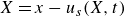 $X=x-u_s(X,t)$
from
$X=x-u_s(X,t)$
from
 $0$
to
$0$
to
 $1$
(dark to light) during one cycle. We distinguish between the loading half of the cycle (
$1$
(dark to light) during one cycle. We distinguish between the loading half of the cycle (
 $\dot {a}\gt 0$
; solid curves) and the unloading half of the cycle (
$\dot {a}\gt 0$
; solid curves) and the unloading half of the cycle (
 $\dot {a}\lt 0$
; dashed curves).
$\dot {a}\lt 0$
; dashed curves).

Appendix B. Analytical solution for molecular diffusion and advection
The analytical solution for the molecular diffusion of a step function in a semi-infinite material, as formulated by Crank (Reference Crank1979), is
 \begin{equation} c(x,t)=c_0 \left \{1- \frac {1}{2} \left [\mathrm {erfc}\left (\frac {l + x -1}{2\sqrt {\mathrm {Pe}^{-1} t}}\right ) +\mathrm {erfc}\left (\frac {l - x +1}{2\sqrt {\mathrm {Pe}^{-1} t}}\right )\right ]\right \}. \end{equation}
For slow loading, the analytical solution for advection only (
 $\mathrm {Pe}^{-1}=\alpha =0$
) is
$\mathrm {Pe}^{-1}=\alpha =0$
) is
 \begin{equation} c({x},t)=\frac {1}{2} \left \{ \tanh { \left [{s}\left ( ({x}-1)\frac {\phi _{f,0}}{\phi _f}+{l}\right ) \right ]} +1 \right \} . \end{equation}
In figure 16, we compare these analytical solutions with the numerical solutions obtained with the method described in Appendix A. Note that, for the case of diffusion, we consider an initial solute profile that is smoother than the one for which the analytical solution is formulated. Hence, the two solutions show an initial discrepancy that vanishes with time, as the profile adjusts towards classical self-similarity.
Evolution of
 $\delta$
and
$\delta$
and
 $\chi$
over 5 cycles for different values for (a,b) the initial porosity
$\chi$
over 5 cycles for different values for (a,b) the initial porosity
 $\phi _{f,0}$
and (c,d) the initial solute stripe width
$\phi _{f,0}$
and (c,d) the initial solute stripe width
 $l$
.
$l$
.

Appendix C. Dispersive flux
In this appendix, we justify the choice of fixing
 $\mathrm {Pe}^{-1}$
and
$\mathrm {Pe}^{-1}$
and
 $\alpha$
to the specific baseline values reported in table 1. We do so by quantifying the strength of dispersion relative to diffusion using the ratio of the dispersive solute flux
$\alpha$
to the specific baseline values reported in table 1. We do so by quantifying the strength of dispersion relative to diffusion using the ratio of the dispersive solute flux
 $ q_{{disp}}$
to the diffusive solute flux
$ q_{{disp}}$
to the diffusive solute flux
 $q_{{diff}}$
which we define as
$q_{{diff}}$
which we define as
 \begin{equation} \frac {q_{{disp}}}{q_{{diff}}}= \alpha \mathrm {Pe}| {v}_f-{v}_s|, \end{equation}
and which measures the relative importance of these two mechanisms. In figure 17, we compare
 $q_{{disp}}/q_{{diff}}$
for the slow-loading and low-amplitude case and for the fast-loading and high-amplitude case. In the former, diffusion prevails over dispersion throughout the domain, while in the latter dispersion is the dominant mechanism. Hence, the specific baseline values chosen for
$q_{{disp}}/q_{{diff}}$
for the slow-loading and low-amplitude case and for the fast-loading and high-amplitude case. In the former, diffusion prevails over dispersion throughout the domain, while in the latter dispersion is the dominant mechanism. Hence, the specific baseline values chosen for
 $\mathrm {Pe}^{-1}$
and
$\mathrm {Pe}^{-1}$
and
 $\alpha$
are such that our results span the range from diffusion-dominated to dispersion-dominated transport across the range of
$\alpha$
are such that our results span the range from diffusion-dominated to dispersion-dominated transport across the range of
 $A$
and
$A$
and
 $T$
considered.
$T$
considered.
Appendix D. Initial porosity and solute strip width
Results of varying
 $\phi _{f,0}$
and
$\phi _{f,0}$
and
 $l$
are shown in figure 18. Decreasing
$l$
are shown in figure 18. Decreasing
 $\phi _{f,0}$
leads to larger oscillations in fluid flux for a given solid velocity (see equation (2.22)) In this way, both advection and hydrodynamic dispersion are enhanced. However, the resulting impact on travel distance in figure 18 is relatively small because dispersion is relatively weak for these parameters.
$\phi _{f,0}$
leads to larger oscillations in fluid flux for a given solid velocity (see equation (2.22)) In this way, both advection and hydrodynamic dispersion are enhanced. However, the resulting impact on travel distance in figure 18 is relatively small because dispersion is relatively weak for these parameters.
Increasing the initial solute amount leads to a sharp increase in the travel distance: this is generally expected because the total concentration of solute is higher and therefore all the transport mechanisms are amplified. In addition, the fluid flux increases monotonically in magnitude from right to left, so larger values of
 $l$
expose the solute front to stronger advection and dispersion. However, note that a wider solute strip is associated with a lower degree of mixing because the variance of the solute compared with the initial variance is lower when there is more solute (see equation 3.3).
$l$
expose the solute front to stronger advection and dispersion. However, note that a wider solute strip is associated with a lower degree of mixing because the variance of the solute compared with the initial variance is lower when there is more solute (see equation 3.3).


 Open access