


1. Introduction
The increasing use of Hybrid and Electric Vehicles (EVs) in recent years, also called quiet vehicles (QVs), has led to safety concerns for pedestrians. Below 40 km/hour, the noise emitted by those vehicles is lower than for internal combustion engine vehicles (ICEVs; Japan Automotive Standards Internationalization Center 2009). In urban environments in particular, this can make it more difficult to detect an approaching vehicle. Visually impaired people are particularly affected, as they rely mostly on auditory cues to assess the presence of vehicles (Konet et al. Reference Konet, Sato, Schiller, Christensen, Tabata and Kanuma2011; Parizet, Ellermeier & Robart Reference Parizet, Ellermeier and Robart2014). Because of this, legislation now exists in several countries, requiring QVs to be equipped with a warning sound generation device (acoustic vehicle alert system), as well as specifications regarding the sound that should be emitted (Lee et al. Reference Lee, Lee, Shin and Han2017). Nevertheless, regulations regarding the sound of electric cars may evolve and their sound design remains widely open. Several studies came up with recommendations regarding the nature of such a sound, based on detection time measurements (Misdariis, Gruson & Susini Reference Misdariis, Gruson and Susini2013; Robart & Parizet Reference Robart and Parizet2013; Parizet et al. Reference Parizet, Ellermeier and Robart2014; Poveda-Martínez et al. Reference Poveda-Martínez, Peral-Orts, Campillo-Davo, Nescolarde-Selva, Lloret-Climent and Ramis-Soriano2017). However, these recommendations should also take into account potential noise pollution that could negatively affect the experience of pedestrians, cyclists and other drivers (Petiot, Kristensen & Maier Reference Petiot, Kristensen and Maier2013).
It is indeed clear that QV sounds may be masked by the background noise of the environment, making them hard to detect. A naive solution which consists of a simple increase of the sound level to reduce the masking effect may have dramatic consequences on sound pollution. Thus, there is a conflict between detectability and annoyance in the perception and design of QV sounds. Different studies addressed this problem (Parizet et al. Reference Parizet, Ellermeier and Robart2014; Singh, Payne & Jennings Reference Singh, Payne and Jennings2014; Lee et al. Reference Lee, Lee, Shin and Han2017; Steinbach & Altinsoy Reference Steinbach and Altinsoy2019). Between 2010 and 2014, the European project eVADER showed that it is possible to design a QV warning sound that is both easily detectable and of a low-amplitude level (Parizet et al. Reference Parizet, Ellermeier and Robart2014). However, these approaches do not allow for an extensive sound space exploration, as the sounds tested are chosen from a fixed, small corpus of artificial sound stimuli.
Furthermore, the design of QV sounds is also crucial from a branding point of view. Though being partially limited by the legislation, a manufacturer should be able to explore a wide range of possibilities, in order to design a sound that will distinguish them from their competitors. In that respect, anticipating customer preferences and predicting the perceived quality is important (Swart, Bekker & Bienert Reference Swart, Bekker and Bienert2018). QV is a rather new product, and its collective representation in terms of sound identity has yet to be defined. This could also be an opportunity to make bold choices about the futuristic image of the vehicle, if that is considered a good selling point. One may also desire a QV sound that is as similar as possible to an ICEV.
The design of QV warning sounds is clearly a multiobjective design problem that is closely related to human auditory perception. The challenge for the sound designer is to understand all the facets of the problem and to translate them into relevant acoustic attributes. In addition to the expertise of a designer (and his/her innovativeness! [Engler Reference Engler2016]), listening tests are required to understand the complex relationships between acoustic parameters and perceptual dimensions (Edworthy, Loxley & Dennis Reference Edworthy, Loxley and Dennis1991). Therefore, to assist designers in their design decisions and to confirm their proposals, an active research field in product design considers the analysis of end users’ perceptions or preference, to extract useful information to make design decisions (Orsborn, Cagan & Boatwright Reference Orsborn, Cagan and Boatwright2009; Bi et al. Reference Bi, Li, Wagner and Reid2017).
The purpose of this paper is to define a tool to guide the design of product sounds. The proposal is based on an interactive genetic algorithm (IGA) because of the potential of such algorithms to interactively take into account feedback from the listeners, and their ability to consider conflicting objectives.
In Petiot, Legeay & Lagrange (Reference Petiot, Legeay and Lagrange2019), a study using an IGA for the design of QV sounds was presented. After a definition of the experimental protocol for the listening tests and the sound synthesis technique, a mono-objective optimisation using IGA was implemented, to explore the trade-off between detectability and unpleasantness, which were aggregated as a weighted sum. The results showed that the sound solutions produced by the IGA were efficient when compared to proposals of a designer. In a following work (Souaille et al. Reference Souaille, Petiot, Lagrange and Misdariis2021), we showed that interesting recommendations can be extracted from the analysis of Pareto efficient QV sounds, provided by a multiobjective IGA experiment (optimisation of detectability and unpleasantness).
This paper is a continuation of these two studies. It uses the same experimental protocol for the assessment of the detectability and the unpleasantness of sounds, but validation experiments are added to demonstrate the efficiency of the proposals.
The general aim of the study is to propose a method based on listening tests and an IGA to assist the design of alert sounds for QVs. A multiobjective IGA is implemented with a panel of participants, in order to produce a set of Pareto efficient solutions. A method is next proposed to define design recommendations, from the analysis of the Pareto set. These recommendations are then compared to other design proposals (provided by a designer, or randomly defined). Two research questions are considered:
-
(i) Q1: At an individual level (for each participant), how do QV sounds designed with the IGA compare to other design proposals, in terms of unpleasantness and detectability?
-
(ii) Q2: How do the design recommendations obtained with the proposed method (by gathering individual data) compare to other design proposals, in terms of unpleasantness and detectability, with an external panel of listeners?
Three experiments are carried out to answer these questions. In Experiment 1, participants are invited to use the IGA paradigm in order to define individual Pareto optimal QV sounds, from which a single ‘best’ sound is selected, for each participant. In Experiment 2, the same participants have to assess their ‘best’ sound, together with other proposals, in order to compare their performances. In Experiment 3, a second panel of participants is invited to assess the recommended designs, together with other design proposals, in order to compare their performances.
The two novel contributions of the work are:
-
(i) the use of an IGA applied to a multiobjective sound design problem;
-
(ii) a solution recommendation method, based on the analysis of the solutions obtained by a group of subjects, who used an IGA applied to a multiobjective problem.
For the design of a QV sound, these tools aim at helping a sound designer, by the proposition of efficient sound examples, or by the tuning of synthesis parameters. The proposed method could be transposed to other sound design problems with multiple conflicting objectives. For example, a self-driving car manufacturer could want to design sounds that continuously inform the passengers of surrounding traffic conditions and driving behaviour, while not being too intrusive or annoying (Misdariis, Cera & Rodriguez Reference Misdariis, Cera and Rodriguez2019; Fagerlönn, Larsson & Maculewicz Reference Fagerlönn, Larsson and Maculewicz2020). More generally, the recommendation method could be applied to any multiobjective design problem dealing with the interactive optimisation of perceptual quantities.
The paper is organised as follows. A short background on the integration of user perceptions in product design is presented in Section 2, together with a description of the multiobjective IGA implementation used in this study. Section 3 presents the sound synthesis method implemented, the listening test scenario and the interfaces. Sections 4–6 are dedicated to the description of the three experiments, with the methods implemented and the analysis of the results. Section 7 proposes a summary of the main results. Section 8 presents and discusses the results of the experiments, and concludes on the hypotheses under study. In Section 9, conclusions are drawn on the main contributions of this paper and recommendations for the design of sounds are made.
2. Background
2.1. Integration of user perceptions
In order to include users’ perception in the design process, two categories of methods can be considered.
The first category of methods to tackle this problem is based on the modelling of users’ perceptions or preferences according to a given set of parameterised products (modelling of perceptual data). These methods use the design of experiments (DOE) theory and assume an explicit model (generally linear without interaction) between the perceptual dimensions and the design variables. Various statistical procedures and experiment designs exist to estimate the coefficients of the model. The Japanese Kansei engineering, a well-known design method to account for users’ feelings and perceptions (Nagamachi Reference Nagamachi1995), belongs to this category. For instance, it is considered in sound design to explore how human feelings and emotions can be evoked by a sound’s physical properties. For warning sounds, many studies proposed an experimental approach with listening tests to understand human perceptions for sound design (Ibrahim, Yiap & Andrias Reference Ibrahim, Yiap and Andrias2018). In Marshall, Lee & Austria (Reference Marshall, Lee and Austria2007), different listening scenarios are proposed to study two objectives, namely annoyance and urgency, with a fixed DOE. Knowing the effect of sound parameters on the perceived urgency is important to give precise recommendations (Edworthy, Loxley & Dennis Reference Edworthy, Loxley and Dennis1991). Another approach consists in testing how classical psychoacoustic metrics (loudness, roughness, fluctuation strength etc.) can explain perceptual assessments (Lee et al. Reference Lee, Lee, Shin and Han2017).
To study and understand human reaction to sounds, experiments generally use a parameterised sound synthesis method and model-based DOE (e.g., D-optimal DOE). The limitation of such an approach is that a model between the acoustic parameters and the perceptual dimension must be assumed in advance, given that the exact form of the model is generally unknown. To reduce the complexity of the models, the sounds proposed in the listening tests are generally simple stimuli that are not representative of the complexity of real design solutions and fail to be relevant for multiple objectives. Furthermore, a systematic exploration of a large sound space can be a tedious task – or even infeasible – and user listening fatigue has to be taken into account.
The second category of methods for the analysis of users’ perceptions is not model-based and uses human–computer interactions. These methods are model-free in content (contrary to DOE, there is no model of the behaviour of the respondent), but model-driven for the solution search. In this case, an algorithm gradually refines the propositions made to the users. In interactive evolutionary computation (IEC) algorithms, for example, the user plays the role of the evaluator in an evolutionary process (Takagi Reference Takagi2001). In IEC, the user assesses the fitness of a design population (which is the adaptation of the population to the problem), by rating the proposed designs or choosing the best ones, for example. IEC has been applied to many domains (music, writing, education, food industry etc.) involving different sensory modalities.
Particular cases of IEC are IGAs, where genetic operators, such as recombination, crossover and mutation, are used to modify the designs throughout the optimisation process. This method has been used, for example, to capture the aesthetic intention of participants for the design of cartoons (Gu, Tang & Frazer Reference Gu, Tang and Frazer2006). IGAs have also been tested in our previous studies for the design of car dashboards (Poirson et al. Reference Poirson, Petiot, Boivin and Blumenthal2013), which have confirmed their relevance for extracting design trends and obtaining a final product solution that optimises a determined semantic dimension. IGAs have the advantage of not needing restrictive assumptions regarding the perceptual model of the participant. Interaction effects are in fact implicitly integrated in the course of the model-driven search in the solution space. IGAs have been used in sound design for musical compositions (Biles Reference Biles2007) or to design sign sounds, with the purpose of communicating a message through a melody (Miki et al. Reference Miki, Orita, Wake and Hiroyasu2006). Subtle perceptual phenomena can be taken into account for the optimisation of products involving sensory constraints, such as the tuning of cochlear implants (Wakefield et al. Reference Wakefield, Van Den Honert, Parkinson and Lineaweaver2005).
Nevertheless, the implementation of IGAs to support sounds design remains rare. The first reason is that the design of products’ sounds is a relatively recent discipline that does not have as well-established guidelines as in visual design, where products can be described by illustrations or advanced 3D models (Eppinger & Ulrich Reference Eppinger and Ulrich2016). Conversely, sounds are immaterial and embedded in time, which makes the definition of prototypes difficult. ‘Sound sketches’, using, for example, voices and gesture (Delle Monache et al. Reference Delle Monache, Rocchesso, Bevilacqua, Lemaitre, Baldan and Cera2018), can be proposed to rough out a design proposal, but their use still remains limited. The second reason is that the design of sounds is critically dependent on the process of listening. According to Özcan & Van Egmond (Reference Özcan and Van Egmond2012), products’ sounds remain mainly based on the subjective experience of the designer because perceptual factors are complex to investigate. Several perceptual dimensions, potentially conflicting, may be elicited when listening to a sound. And even if generic tools based on a shared vocabulary and sound examples can be proposed (Carron et al. Reference Carron, Rotureau, Dubois, Misdariis and Susini2017), their adaptation to a particular project remains difficult.
Comparisons of IGA and classical DOE are rare in the engineering design literature. DOE allows for the definition of optimal products, the estimate of effects of factors on the response and the generation of predictions in the design space (with the model), while IGA is only oriented towards the search for the optimal product. A comparison of IGA and fractional factorial design for the design of warning sounds is presented in Petiot et al. (Reference Petiot, Villa, Denjean and Diaz2020). Results show that the IGA method can be an interesting alternative to classical DOE to help the design of sounds. Another comparative study concerns the design of the shape of a bottle using Conjoint Analysis, where the authors conclude on the superiority of interactive evolutionary algorithms on fractional DOE to elicit the optimum product, but without explanations for the reasons behind this superiority (Teichert & Shehu Reference Teichert and Shehu2007).
2.2. Multiobjective IGA
Genetic algorithms take inspiration from some knowledge of the evolutionary process of living organisms to solve optimisation problems (Goldberg Reference Goldberg1989). Potential solutions to a given problem are coded as strings of numbers called chromosomes. A chromosome is composed of several sections, called genes, each coding the values of different parameters of the corresponding solution. Solutions are evaluated in groups, called generations, usually using a fitness function. At each generation, a mating pool is created based on previous solutions’ performances with respect to the problem’s objectives. So-called genetic operators are applied to the solutions within that mating pool to create the next generation of solutions that will be evaluated. This process is repeated until convergence is achieved or the maximum number of generations is reached.
In IGAs, the evaluation of the solutions (fitness) is done by a human, so the fitness function does not have a mathematical expression. With this approach, it is possible to find solutions to problems involving a semantic dimension (such as the notion of ‘unpleasantness’ in this study, or the ‘clearance’ of a car dashboard in Poirson et al. Reference Poirson, Petiot, Boivin and Blumenthal2013), or perceptual dimensions. IGA can be used to assist the design of hearing aids (Durant et al. Reference Durant, Wakefield, Tasell and Rickert2004) or to optimise the affordances of steering wheels (Mata et al. Reference Mata, Fadel, Garland and Zanker2018). In this type of procedure, user fatigue is the main limitation to the maximum number of possible evaluations. This limits both the number of solutions per generation as well as the number of generations, which has an impact on the convergence of the algorithm. What is more, for time-varying solutions such as sounds, only one solution can be evaluated at a time.
The optimisation problem addressed in this paper is bi-objective, which means that there are potentially several equally satisfying solutions (Pareto efficient). To address this constraint, the proposed method considers an adaptation of the NSGA-II algorithm (Nondominated Sorting Genetic Algorithm II; Deb et al. Reference Deb, Pratap, Agarwal and Meyarivan2002), which aims at finding an approximation of the optimal Pareto front of the potential solutions. A Pareto front comprises the solutions that are nondominated in the Pareto sense. A solution is said to Pareto-dominate another one if it is better or equal to this solution for all objectives and if there is at least one objective where it is strictly better. An example of this is shown in Figure 1, where solutions are represented according to two objectives that must be minimised. The group of nondominated solutions is called the Pareto front. By ignoring the solutions of the Pareto front, it is possible to find the second front (Rank 2) of nondominated solutions, and so on. Figure 1b shows an example of the Pareto front (Rank 1) and other successive ranks.
Example of Pareto domination for a bi-objective problem where both objectives have to be minimised. In (a), the black square Pareto dominates the white squares. In (b), the nondomination ranks are shown.
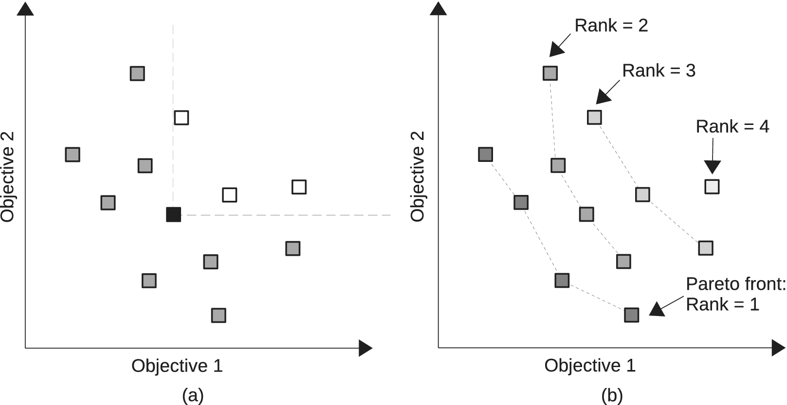
In the NSGA-II algorithm, the solutions are compared based on the so-called crowded-comparison operator. A solution is considered better than another one if it has a lower (closer to 1) nondomination rank. The nondomination rank of a solution corresponds to the nondominated front it belongs to. Within a nondominated front, the solutions are ranked based on their distances to other solutions of the same front in the objective space. Solutions that are further away from other solutions are considered better. This aims at ultimately obtaining solutions that are evenly spread along the optimal Pareto front.
In this elitist algorithm, a register of the best solutions evaluated is updated after each generation and is used to create the following one. This register has the same size
 $ N $
as the number of solutions in a generation’s population. After each evaluation of a generation of
$ N $
as the number of solutions in a generation’s population. After each evaluation of a generation of
 $ N $
solutions, the register is updated by keeping the best
$ N $
solutions, the register is updated by keeping the best
 $ N $
solutions amongst the union of the
$ N $
solutions amongst the union of the
 $ N $
solutions in the current generation and the
$ N $
solutions in the current generation and the
 $ N $
solutions that are currently in the register. At the first generation, the register being empty, it is initialised with all
$ N $
solutions that are currently in the register. At the first generation, the register being empty, it is initialised with all
 $ N $
solutions within the population.
$ N $
solutions within the population.
2.3. Implementation of the IGA
Our implementation uses the NSGA-II algorithm (Deb et al. Reference Deb, Pratap, Agarwal and Meyarivan2002). The procedure is implemented as follows: the first generation of
 $ N $
solutions is generated using a Latin Hypercube Sample. After evaluation by the user, the best-solution register is initialised with all
$ N $
solutions is generated using a Latin Hypercube Sample. After evaluation by the user, the best-solution register is initialised with all
 $ N $
solutions of this first generation. The next generation is created by randomly applying one of the following genetic operators to each solution within the register, which constitutes the mating pool:
$ N $
solutions of this first generation. The next generation is created by randomly applying one of the following genetic operators to each solution within the register, which constitutes the mating pool:
-
(i) Mutation: the solution is replicated to the next generation, with one gene value randomly changed.
-
(ii) Crossover: another solution is selected within the register through a binary tournament based on the crowded-comparison operator. The chromosomes representing the two solutions are combined, in order to create a new one. This is done by randomly selecting a chromosome location, splitting each chromosome into two parts around that location and connecting the first part of one solution with the second part of the other one. The order in which the solutions are combined is chosen randomly.
-
(iii) Selection: the solution is replicated in the next generation without any modification.
The probability for each operator to be applied is defined by a rate
 $ {m}_r $
,
$ {m}_r $
,
 $ {c}_r $
and
$ {c}_r $
and
 $ {s}_r $
, corresponding to mutation, crossover and selection, respectively. These rates are normalised so that they add up to 1, that is,
$ {s}_r $
, corresponding to mutation, crossover and selection, respectively. These rates are normalised so that they add up to 1, that is,
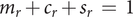 $ {m}_r+{c}_r+{s}_r\hskip0.35em =\hskip0.35em 1 $
.
$ {m}_r+{c}_r+{s}_r\hskip0.35em =\hskip0.35em 1 $
.
To select which operator to apply, a number
 $ r $
is randomly generated between 0 and 1:
$ r $
is randomly generated between 0 and 1:
-
(i) If
 $ 0\hskip0.35em \le \hskip0.35em r\hskip0.35em \le \hskip0.35em {m}_r $
, a mutation is applied.
$ 0\hskip0.35em \le \hskip0.35em r\hskip0.35em \le \hskip0.35em {m}_r $
, a mutation is applied. -
(ii) If
$ {m}_r<r\hskip0.35em \le \hskip0.35em {m}_r+{c}_r $
, a crossover with another solution is applied. -
(iii) If
$ {m}_r+{c}_r<r\hskip0.35em \le \hskip0.35em 1 $
, a selection is applied.


This process is repeated at each generation. The size of the register is kept constant, only containing the
 $ N $
best solutions.
$ N $
best solutions.
The same solution (sound) can thus be evaluated several times during the optimisation process, and some variability is expected with regard to the evaluation of the two objectives by the subject. Thus, there is a risk that the best-solution register would contain several times the same sound, with different objective values. This would reduce diversity in the mating pool, which could lead to a premature convergence. To prevent this, each solution in the register is only present once, associated with the latest evaluation that the subject provided for this sound.
3. Sound synthesis and experimental protocol
3.1. QV sound synthesis
The QV sounds are synthesised using the additive synthesis technique (Roads Reference Roads1996). By considering an analysis of current sounds of different carmakers (Misdariis et al. Reference Misdariis, Cera, Levallois and Locqueteau2012) and personal propositions (Petiot et al. Reference Petiot, Kristensen and Maier2013), the generation of different but plausible sounds for an electric car includes two types of sounds: (1) a ‘harmonic’ sound (discrete distribution of energy with respect to frequency – the frequencies being multiple of a fundamental) and (2) a noise sound (continuous distribution of energy with respect to frequency). The ‘harmonic’ sound is made of two components: a motor sound (
 $ {C}_1 $
), mimicking a combustion engine, and a major chord (
$ {C}_1 $
), mimicking a combustion engine, and a major chord (
 $ {C}_2 $
), giving a tonal component. The noise sound is also made of two independent noise bands (
$ {C}_2 $
), giving a tonal component. The noise sound is also made of two independent noise bands (
 $ {C}_3 $
and
$ {C}_3 $
and
 $ {C}_4 $
). More formally:
$ {C}_4 $
). More formally:
-
(i)
$ {C}_1 $
, the engine-like sound, is simulated with a weighted sum of harmonics corresponding to a four-cylinder internal combustion engine (ICE; with RPM the rotation speed of the motor (tr/mn), the fundamental frequency is given by
$ {f}_1\hskip0.35em =\hskip0.35em \frac{RPM}{60} $
).


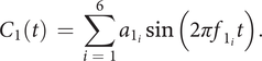 $$ {C}_1(t)\hskip0.35em =\hskip0.35em \sum \limits_{i\hskip0.35em =\hskip0.35em 1}^6{a}_{1_i}\sin \left(2\pi {f}_{1_i}t\right). $$
Six subharmonics or harmonics are considered
 $ {f}_{1_i}\in \left\{0.5{f}_1,{f}_1,\mathrm{1.5}{f}_1,2{f}_1,4{f}_1,6{f}_1\right\} $
with the corresponding amplitudes
$ {f}_{1_i}\in \left\{0.5{f}_1,{f}_1,\mathrm{1.5}{f}_1,2{f}_1,4{f}_1,6{f}_1\right\} $
with the corresponding amplitudes
 $ {a}_{1_i}\in \left\{\mathrm{0.2,0.4,0.5,0.2,0.4,0.6}\right\} $
(see Desoeuvre et al. Reference Desoeuvre, Richard, Roussarie and Bezat2008 for more information on the acoustics of thermal engines).
$ {a}_{1_i}\in \left\{\mathrm{0.2,0.4,0.5,0.2,0.4,0.6}\right\} $
(see Desoeuvre et al. Reference Desoeuvre, Richard, Roussarie and Bezat2008 for more information on the acoustics of thermal engines).
-
(ii)
$ {C}_2 $
, the major chord, is made of three harmonic (periodic) notes (root note [fundamental frequency
$ {f}_2 $
], major third [
$ \frac{5}{4}{f}_2 $
] and fifth [
$ \frac{3}{2}{f}_2 $
]). Each note is composed of six harmonics (e.g., for the root note, harmonics
$ {f}_{2_i}\in \left\{{f}_2,2{f}_2,3{f}_2,4{f}_2,5{f}_2,6{f}_2\right\} $
with the corresponding amplitudes
$ {a}_{2_i}\in \left\{\mathrm{1,0.4,0.4,0.1,0.1,0.1}\right\} $
),


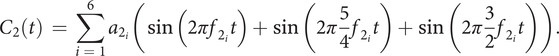 $$ {C}_2(t)\hskip0.35em =\hskip0.35em \sum \limits_{i\hskip0.35em =\hskip0.35em 1}^6{a}_{2_i}\left(\sin \left(2\pi {f}_{2_i}t\right)+\sin \left(2\pi \frac{5}{4}{f}_{2_i}t\right)+\sin \left(2\pi \frac{3}{2}{f}_{2_i}t\right)\right). $$
-
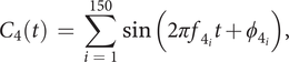
(iii)
$ {C}_3 $
, the first noise component, is built as a sum of 150 sines with random phase and frequency,

 $$ {C}_3(t)\hskip0.35em =\hskip0.35em \sum \limits_{i\hskip0.35em =\hskip0.35em 1}^{150}\sin \left(2\pi {f}_{3_i}t+{\phi}_{3_i}\right), $$
with
 $ {f}_{3_i}\in \left[0,2{f}_3\right] $
and
$ {f}_{3_i}\in \left[0,2{f}_3\right] $
and
 $ {\phi}_{3_i}\in \left[0,2\pi \right] $
.
$ {\phi}_{3_i}\in \left[0,2\pi \right] $
.
-
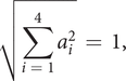
(iv)
$ {C}_4 $
, the second noise component, is identical to
$ {C}_3 $
, but with another frequency range. The frequency
$ {f}_4 $
is chosen so that
$ {C}_4 $
has a wider frequency range than
$ {C}_3 $
,


 $$ {C}_4(t)\hskip0.35em =\hskip0.35em \sum \limits_{i\hskip0.35em =\hskip0.35em 1}^{150}\sin \left(2\pi {f}_{4_i}t+{\phi}_{4_i}\right), $$
with
 $ {f}_{4_i}\in \left[0,2{f}_4\right] $
and
$ {f}_{4_i}\in \left[0,2{f}_4\right] $
and
 $ {\phi}_{4_i}\in \left[0,2\pi \right] $
.
$ {\phi}_{4_i}\in \left[0,2\pi \right] $
.
The resulting sound
 $ s(t) $
is the weighted sum of these four components, to which amplitude modulation is applied, with modulation index
$ s(t) $
is the weighted sum of these four components, to which amplitude modulation is applied, with modulation index
 $ m $
and modulation frequency
$ m $
and modulation frequency
 $ {f}_m $
:
$ {f}_m $
:
 $$ s(t)\hskip0.35em =\hskip0.35em (1+m\cdot \mathrm{sin}(2{\pi f}_mt))\cdot ({a}_1\cdot {C}_1(t)+{a}_2\cdot {C}_2(t)+{a}_3\cdot {C}_3(t)+{a}_4\cdot {C}_4(t)). $$
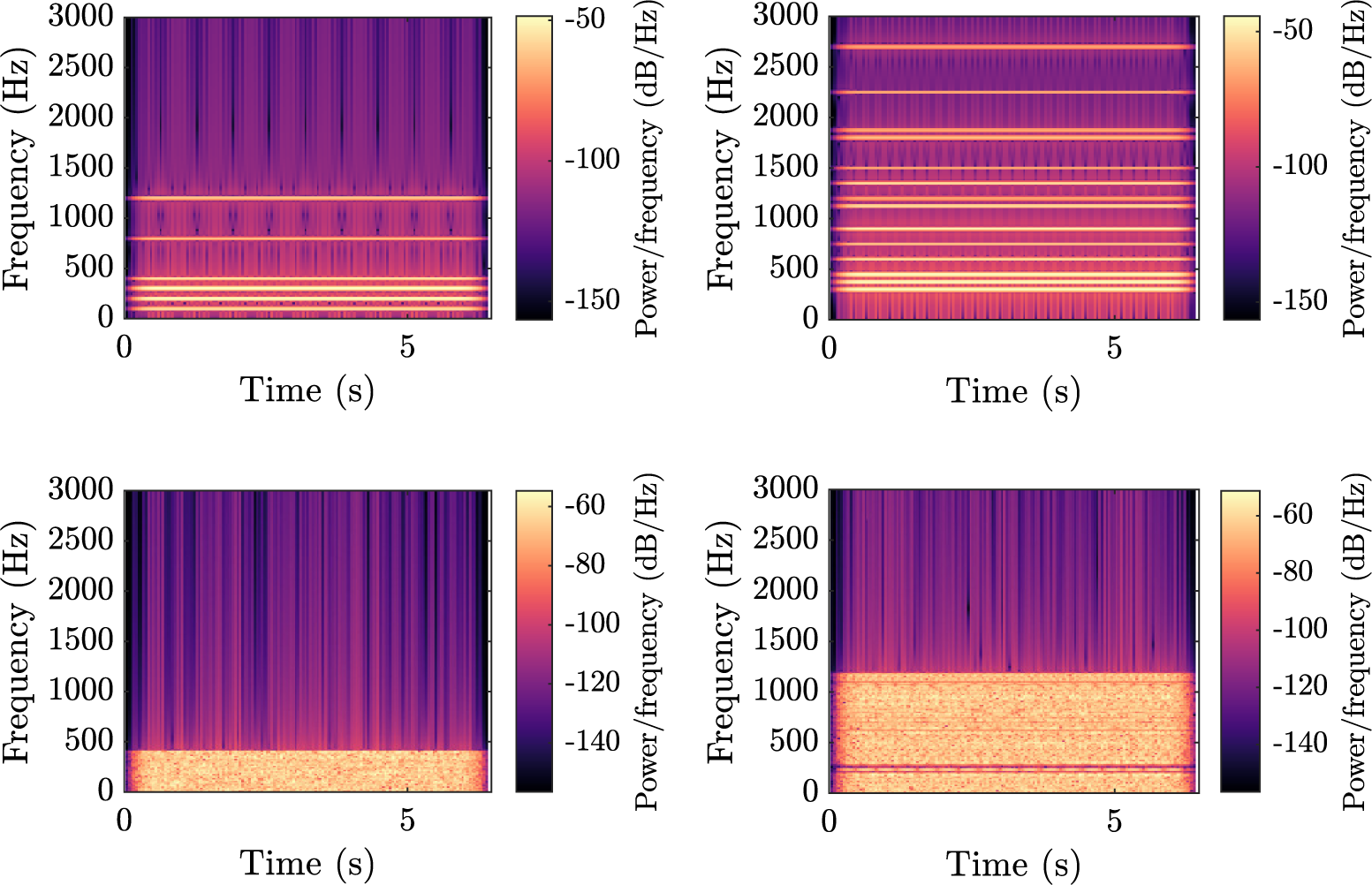
The four amplitude coefficients
 $ {a}_i $
are normalised so that
$ {a}_i $
are normalised so that
 $$ \sqrt{\sum \limits_{i\hskip0.35em =\hskip0.35em 1}^4{a}_i^2}\hskip0.35em =\hskip0.35em 1, $$
and the ratio between
 $ {a}_3 $
and
$ {a}_3 $
and
 $ {a}_4 $
is chosen equal to
$ {a}_4 $
is chosen equal to
 $ 0.5 $
.
$ 0.5 $
.
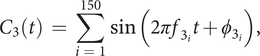
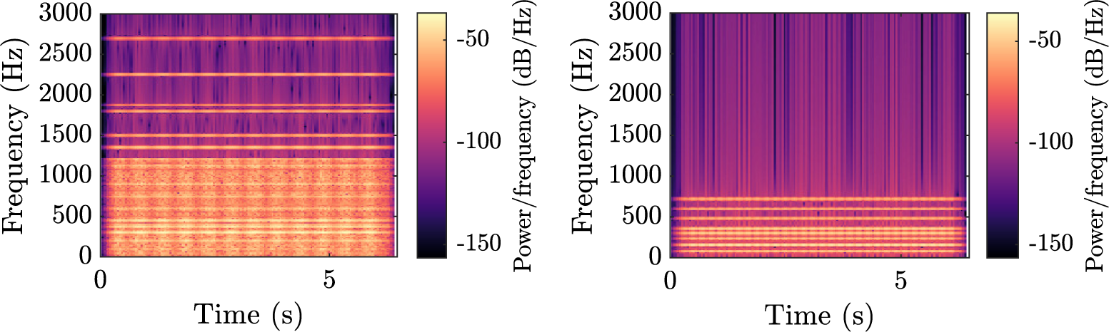
Figure 2 illustrates each component by showing spectrograms (representation of the evolution of the spectrum of the signal with respect to time) of a sample, for a vehicle driving at constant speed. The horizontal stripes in the top spectrograms denote a harmonic structure made of pure sinusoids, whereas the wide horizontal bands in the bottom plots indicate noise. There is no variation over the horizontal axis, because the sounds are stationary, apart from a short fade in and fade out. Example of sounds can be listened to at https://mathieulagrange.github.io/souaille2021interactive/.
Spectrograms of the four synthesiser components, without amplitude modulation. Top-left:
 $ {C}_1 $
motor sound, with
$ {C}_1 $
motor sound, with
 $ {f}_1=200 $
Hz. Top-right:
$ {f}_1=200 $
Hz. Top-right:
 $ {C}_2 $
chord sound, with
$ {C}_2 $
chord sound, with
 $ {f}_2=300 $
Hz. Bottom-left:
$ {f}_2=300 $
Hz. Bottom-left:
 $ {C}_3 $
first noise, with
$ {C}_3 $
first noise, with
 $ {f}_3=200 $
Hz. Bottom-right:
$ {f}_3=200 $
Hz. Bottom-right:
 $ {C}_4 $
second noise, with
$ {C}_4 $
second noise, with
 $ {f}_4=600 $
Hz. The brighter the colour, the more power there is in the corresponding time–frequency bin.
$ {f}_4=600 $
Hz. The brighter the colour, the more power there is in the corresponding time–frequency bin.
The definition of the structure of the synthesised sound and the choice of the variables is the result of many tests, innovative proposals and sound engineering experience of the authors. A complete justification is out of the scope of this paper, the contribution being centred on the optimisation of a given parameterised synthesiser. It is out of the scope of this paper to describe all the parameters of the synthesiser (there are more than 70 independent parameters to define a sound). We can mention that all the frequencies and amplitudes of the components are adjustable, to create credible and original sounds. The synthesiser is controlled by the speed of the car. In this study, this parameter is irrelevant given that the listening tests are made with a constant speed of the car. Readers interested by the design of synthesised QV sounds may consult Pedersen et al. (Reference Pedersen, Gadegaard, Kjems and Skov2011) or Petiot et al. (Reference Petiot, Kristensen and Maier2013) for more information on the evolution of the sound according to speed.
Among the different synthesis parameters of the sounds, it is necessary to define the optimisation variables of the problem, that is, the variables that are manipulated by the IGA and coded in the genome (design space of the genetic code). After several experiments, the following six factors (A, B, C, D, E and F), and their corresponding levels (A1 for Level 1 of Factor A), are chosen to get a large diversity of sounds (see Table 1). These factors control the frequency content and the amplitudes of the synthesiser components, as well as the amplitude and frequency of the amplitude modulation. The choice of the factors is motivated by previous findings showing that harmonic complexity and amplitude modulation are related to detectability (Parizet et al. Reference Parizet, Ellermeier and Robart2014).
Description of the design factors manipulated by the IGA. The values correspond to a speed vehicle of 20 km/hour.
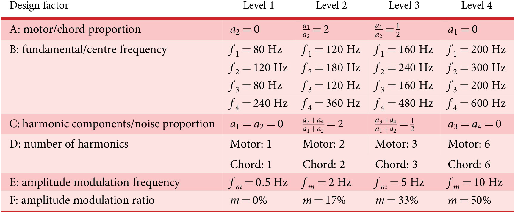
Furthermore, it has been shown that the preference for an EV sound can be related to how similar it is to an ICE car sound (Petiot et al. Reference Petiot, Kristensen and Maier2013). To take that into account, the synthesis method is able to create sounds that resemble more or less an ICE car sound, depending on the value of Factor A. The setting of the levels of the factors required many adjustments (not reported here) to obtain audible differences between sounds, but with still ‘convenient’ sounds. The values of the levels correspond to a speed of 20 km/hour (the speed used for the listening test).
Figure 3 shows the spectrogram of two examples of QV sounds with a constant speed of 20 km/hour, with amplitude modulation, which results in alternating brighter and darker vertical bands. The levels of the factors for these examples are (A3, B4, C3, D4, E2, F4) (left) and (A2, B3, C4, D2, E3, F3) (right). For the first one, this corresponds to:
-
(i)
$ {a}_1\hskip0.35em =\hskip0.35em 0.4 $
,
$ {a}_2\hskip0.35em =\hskip0.35em 0.8 $
,
$ {a}_3\hskip0.35em =\hskip0.35em 0.2 $
and
$ {a}_4\hskip0.35em =\hskip0.35em 0.4 $
(from A3 and C3); -
(ii)
$ {f}_1\hskip0.35em =\hskip0.35em 200 $
Hz,
$ {f}_2\hskip0.35em =\hskip0.35em 300 $
Hz,
$ {f}_3\hskip0.35em =\hskip0.35em 200 $
Hz and
$ {f}_4\hskip0.35em =\hskip0.35em 600 $
Hz (B4); -
(iii) Five harmonics for the motor and five for the chord (D4);
-
(iv)
$ {f}_m\hskip0.35em =\hskip0.35em 2 $
Hz and
$ m\hskip0.35em =\hskip0.35em 50 $
% (E2 and F4).


Spectrogram of the complete sounds synthesised with parameters (A3, B4, C3, D4, E2, F4) (left) and (A2, B3, C4, D2, E3, F3) (right) with a constant speed vehicle (addition of the four synthesised components, with amplitude modulation).
For the second one, this corresponds to:
-
(i)
$ {a}_1\hskip0.35em =\hskip0.35em 0.89 $
,
$ {a}_2\hskip0.35em =\hskip0.35em 0.45 $
,
$ {a}_3\hskip0.35em =\hskip0.35em 0 $
and
$ {a}_4\hskip0.35em =\hskip0.35em 0 $
(from A2 and C4); -
(ii)
$ {f}_1\hskip0.35em =\hskip0.35em 160 $
Hz,
$ {f}_2\hskip0.35em =\hskip0.35em 240 $
Hz,
$ {f}_3\hskip0.35em =\hskip0.35em 160 $
Hz and
$ {f}_4\hskip0.35em =\hskip0.35em 480 $
Hz (B3); -
(iii) One harmonic for the motor and five for the chord (D2);
-
(iv)
$ {f}_m\hskip0.35em =\hskip0.35em 5 $
Hz and
$ m\hskip0.35em =\hskip0.35em 33 $
% (E3 and F3).


3.2. Listening test scenario
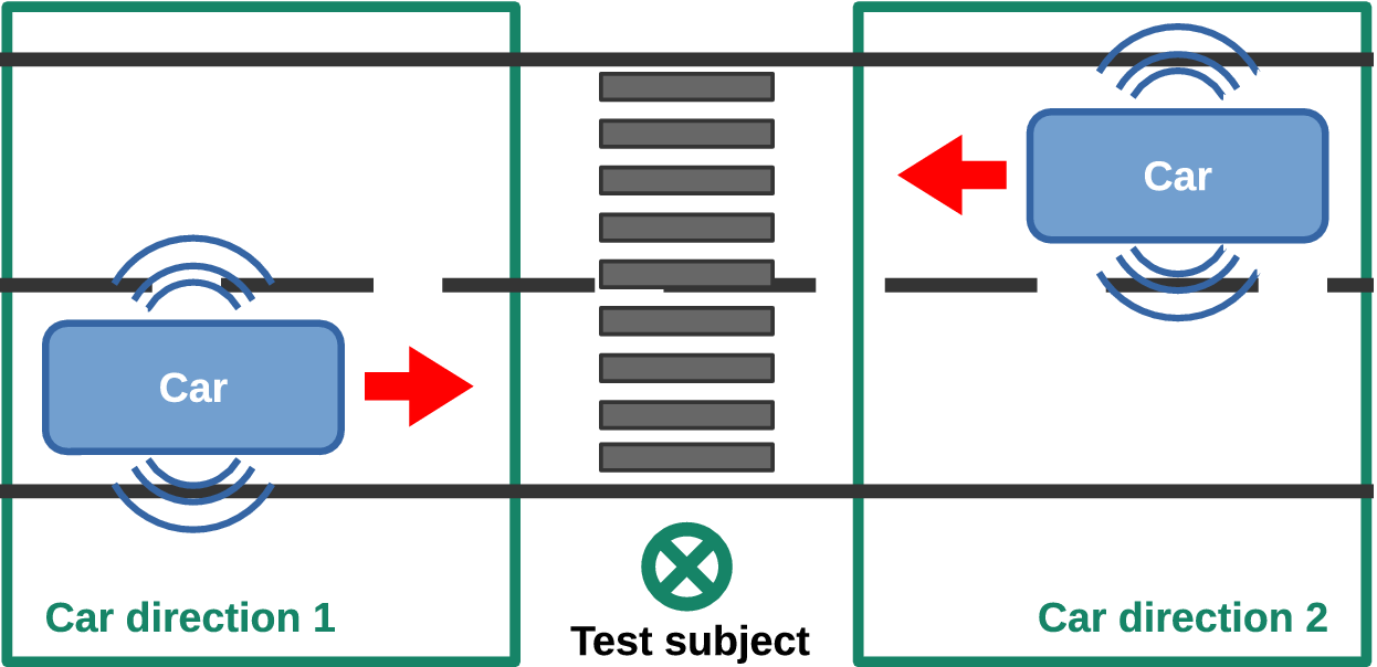
The experiment aims at evaluating the unpleasantness and the detectability of QV sounds. To this end, the following scenario is considered: a pedestrian, standing on the sidewalk of a street, waits before crossing (see Figure 4). A QV may pass by, coming either from the right or from the left. The listener is static, and must indicate when he/she detects the QV. For all the passages, the speed of the car is kept constant (20 km/hour) and the direction of the car is randomly chosen as left or right.
Passing-by scenario for the listening test: pedestrian located on the sidewalk of a street.
To improve the realism of the test, the car sound is mixed with a urban environment background, made from a stereo street recording of a busy intersection in Paris, France. To be used as background noise, the soundscape must be amorphous (Maffiolo Reference Maffiolo1999) and not contain any perceivable emergent event (horns, car passing etc.; Kerber & Fastl Reference Kerber and Fastl2008). For this, distracting sounds and close vehicle sounds that could be mistaken for the QV warning sound to evaluate are edited out of the recording. To avoid the potential fatigue of the participant due to the repetition of the exact same background noise during the test, the part of the audio file selected (around 10 seconds) is randomly chosen among the 42-second long recording.
To increase the level of immersion of the listener, and to obtain a more realistic passing-by scenario, the following properties have been implemented for the design of the sound stimuli:
-
(i) The sound level of the QV is modulated according to the vehicle/listener distance. The model used, based on acoustic theory, considers the QV as a monopole and provides a sound level inversely proportional to the distance to the listener (
$ \frac{1}{r} $
; see Figure 5). -
(ii) The Doppler effect is simulated with a shifting in frequency due to the moving source.
-
(iii) The left/right panning of the QV sound is controlled in such a way that the source goes progressively from one canal (left or right, depending of the direction of the QV) to the other (right or left) according to the position of the vehicle. The amplitude panning is controlled using a sine law (Pulkki Reference Pulkki2001).

Timeline of the mix of the background and the quiet vehicle (QV) sound, with their respective amplitude-level evolution (the x-axis represents indifferently the time or the distance of the QV, given that the speed of the vehicle is constant). Note the asymmetry of the amplitude relatively to the listening point.

For the sake of simplicity, the simulation does not include other sound sources, such as tire noise.
In order to reduce the duration of each evaluation, the attenuation function of the QV sound is asymmetrical (reduction in
 $ \frac{1}{r^2} $
once the car passed in front of the listener), as in Misdariis et al. (Reference Misdariis, Gruson and Susini2013), that is, the attenuation is faster than the increase of the sound level. This choice does not affect the detectability of the QV sound, which always occurs in the approach phase. We assume that this asymmetry does not have any effect on the assessments of unpleasantness.
$ \frac{1}{r^2} $
once the car passed in front of the listener), as in Misdariis et al. (Reference Misdariis, Gruson and Susini2013), that is, the attenuation is faster than the increase of the sound level. This choice does not affect the detectability of the QV sound, which always occurs in the approach phase. We assume that this asymmetry does not have any effect on the assessments of unpleasantness.
The scenario’s timeline is shown in Figure 5. The total duration of each sound stimulus is around 10 seconds.
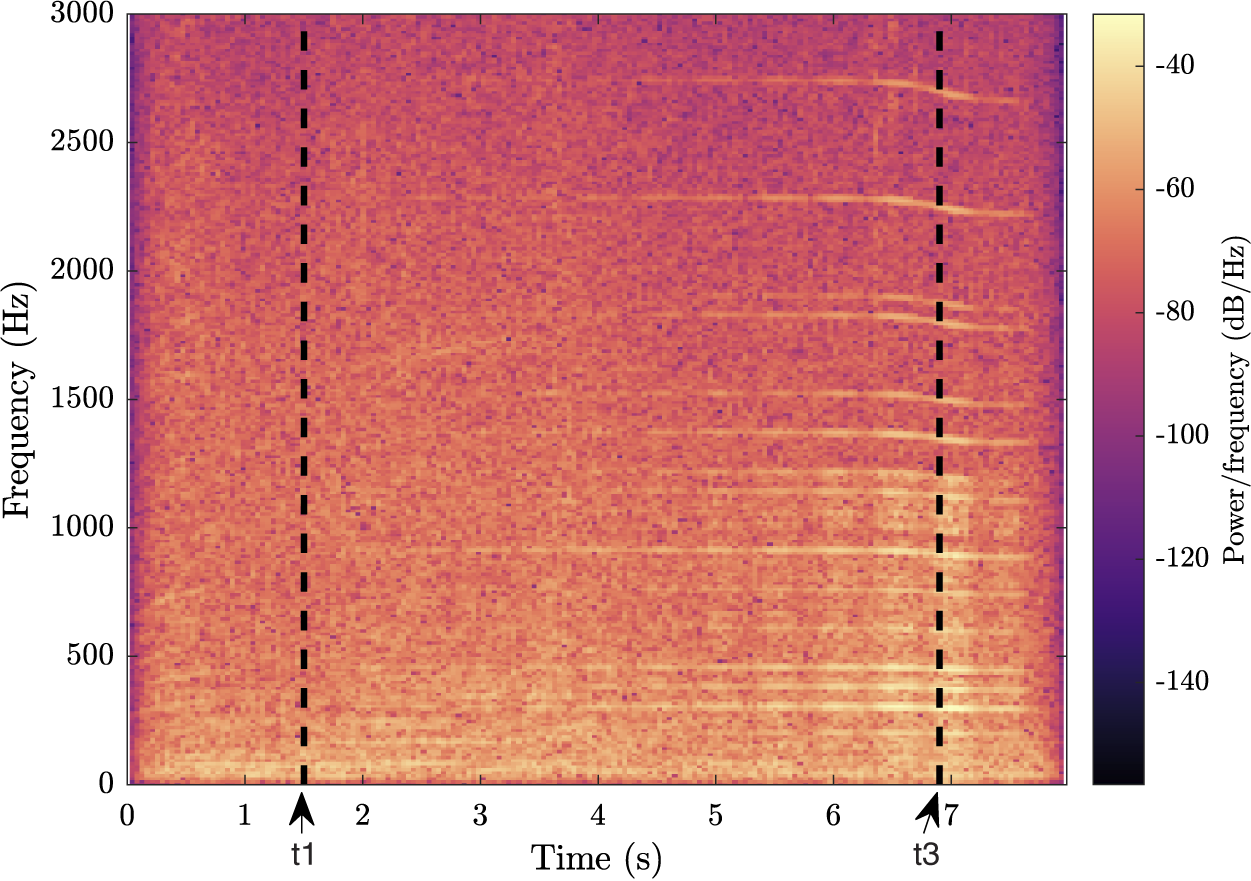
Figure 6 shows the spectrogram of the previous QV sound (A3, B4, C3, D4, E2, F4; Figure 3), now spatialised and mixed with the background noise. The masking of the warning sound by the background is illustrated by the fact that the horizontal stripes only appear some time after
 $ {t}_1 $
. The shifting in frequency, due to the Doppler effect, is visible after time
$ {t}_1 $
. The shifting in frequency, due to the Doppler effect, is visible after time
 $ {t}_3 $
, corresponding to the listener position. The sound can be listened to at https://mathieulagrange.github.io/souaille2021interactive/.
$ {t}_3 $
, corresponding to the listener position. The sound can be listened to at https://mathieulagrange.github.io/souaille2021interactive/.
Spectrogram of an example of a quiet vehicle sound, spatialised and mixed with the background. Time
 $ {t}_1 $
is the time at which the vehicle warning sound starts, and time
$ {t}_1 $
is the time at which the vehicle warning sound starts, and time
 $ {t}_3 $
is the moment the vehicle passes in front of the listener. The horizontal stripes correspond to the harmonic content of the warning sound, progressively emerging from the background.
$ {t}_3 $
is the moment the vehicle passes in front of the listener. The horizontal stripes correspond to the harmonic content of the warning sound, progressively emerging from the background.
3.3. Test procedure and interface
The participants listened to the scenarios using computers and Beyerdynamics DT-990 headphones. The sound level was calibrated so that the background sound is around 69 dBA, when measured with a sound-level meter at the headphone’s output. This level was chosen to be consistent with the dBA level measured during the recording of the background. The warning sound level relative to the background was manually adjusted to avoid having too many sounds detected too early or too late. The mean levels of the warning sounds ranged from 59 dBA to 80 dBA, with 95% of the sounds in the design space having values above 68 dBA (5th percentile).
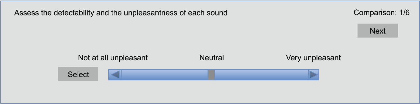
The interface for the assessments of the QV sound is shown in Figure 7. After clicking on the ‘Select’ button, which launches the synthesis of the sound, participants had to strike the ‘space bar’ to start playing the sound. This corresponds to the definition of time
 $ {t}_0 $
(see Figure 5). Next, they had to strike on the keyboard the ‘a’ key as soon as they detect the QV coming from the left, or the ‘e’ key if it is coming from the right (French AZERTY keyboard). This strike allows the definition of the detection time
$ {t}_0 $
(see Figure 5). Next, they had to strike on the keyboard the ‘a’ key as soon as they detect the QV coming from the left, or the ‘e’ key if it is coming from the right (French AZERTY keyboard). This strike allows the definition of the detection time
 $ {t}_2 $
. To avoid habituation of the participant in the detection time (and detect inconsistent subjects), the starting time
$ {t}_2 $
. To avoid habituation of the participant in the detection time (and detect inconsistent subjects), the starting time
 $ {t}_1 $
of the QV sound in the mixture was variable, randomly chosen in the interval [1, 3] seconds. Of course, given this small interval, the event is highly predictable. A larger interval was not reasonable, as it would have increased the duration of the test. Hence, the protocol provides an estimate of the lower bound of the detection time, because it is clear that in real-life situation, when people do not wait for the arrival of a car, the detection time would be larger. This lower bound of the detection time is considered as representative of the detectability of the sound of the car.
$ {t}_1 $
of the QV sound in the mixture was variable, randomly chosen in the interval [1, 3] seconds. Of course, given this small interval, the event is highly predictable. A larger interval was not reasonable, as it would have increased the duration of the test. Hence, the protocol provides an estimate of the lower bound of the detection time, because it is clear that in real-life situation, when people do not wait for the arrival of a car, the detection time would be larger. This lower bound of the detection time is considered as representative of the detectability of the sound of the car.
Interface for the assessment of the detectability and the unpleasantness of a quiet vehicle sound (structured rating scale).
The detection time is then given by
 $$ {D}_t\hskip0.35em =\hskip0.35em {t}_2-{t}_1. $$
If the subject pressed a key before the vehicle warning sound is actually playing, that is, before
 $ {t}_1 $
, the detection time of the sound is changed by default to an arbitrary value (average between the minimum and maximum possible values for the detection time [
$ {t}_1 $
, the detection time of the sound is changed by default to an arbitrary value (average between the minimum and maximum possible values for the detection time [
 $ \frac{t_1+{t}_3}{2} $
]), and a warning was recorded. If the car was not detected or detected too late, that is, after time
$ \frac{t_1+{t}_3}{2} $
]), and a warning was recorded. If the car was not detected or detected too late, that is, after time
 $ {t}_3 $
, the detection time was set to
$ {t}_3 $
, the detection time was set to
 $ {t}_3 $
, that is, the time at which the car passes in front of the subject, and a warning was recorded. If the subject made a mistake when assessing the arrival direction of the car, no action was taken, but a warning was recorded. This random change in the direction of the car is very important in the protocol to be able to detect ‘false alarms’ or ‘wrong detections’, in order to check the reliability of the assessments. The detection time can be converted into the distance to pedestrian using
$ {t}_3 $
, that is, the time at which the car passes in front of the subject, and a warning was recorded. If the subject made a mistake when assessing the arrival direction of the car, no action was taken, but a warning was recorded. This random change in the direction of the car is very important in the protocol to be able to detect ‘false alarms’ or ‘wrong detections’, in order to check the reliability of the assessments. The detection time can be converted into the distance to pedestrian using
 $ V $
, the speed of the car. The distance to pedestrian
$ V $
, the speed of the car. The distance to pedestrian
 $ {D}_p $
at the time of the detection is then given by
$ {D}_p $
at the time of the detection is then given by
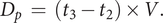 $$ {D}_p\hskip0.35em =\hskip0.35em \left({t}_3-{t}_2\right)\times V. $$
With the distance to pedestrian, a safety zone can be defined given the stopping distance of the car. The stopping distance of a car on a dry road is around 7.5 m at 20 km/hour. Thus, distances to pedestrian
 $ {D}_p $
lower than 7.5 m are considered as dangerous. This corresponds to a detection time
$ {D}_p $
lower than 7.5 m are considered as dangerous. This corresponds to a detection time
 $ {D}_t $
greater than 4.05 seconds.
$ {D}_t $
greater than 4.05 seconds.
After listening to the sound clip, the participants had to evaluate the unpleasantness of the sound on a continuous structured semantic scale going from ‘0’ (‘Not at all unpleasant’) to ‘10’ (‘Very unpleasant’) using a slider as shown in Figure 7. To explain the semantic dimension of unpleasantness, the following information is given to the participants. ‘If the car passed by your house during a calm moment, how unpleasant would the sound be?’
Participants were able to replay the stimuli to assess the unpleasantness (as many times as required), but not to assess detectability. Indeed, they had already heard the sound and knew the direction of arrival of the car.
In the beginning of the test, the subjects were presented with a tutorial, so that they could familiarise themselves with the interface and understand which type of sounds they should pay attention to.
4. Experiment 1: IGA
4.1. Materials and method
For the first experiment, 32 students (16 males and 16 females) from the École Centrale de Nantes, France, with no reported auditory deficiencies, used the IGA procedure. They evaluated 11 generations of 9 sounds (99 sounds), which took approximately half an hour. Values of
 $ {m}_r\hskip0.35em =\hskip0.35em 0.7 $
,
$ {m}_r\hskip0.35em =\hskip0.35em 0.7 $
,
 $ {c}_r\hskip0.35em =\hskip0.35em 0.25 $
and
$ {c}_r\hskip0.35em =\hskip0.35em 0.25 $
and
 $ {s}_r\hskip0.35em =\hskip0.35em 0.05 $
were used for the IGA. A high mutation rate is chosen, to preserve diversity in spite of the small number of individuals per generation and to avoid premature convergence. At the end of the test, for each participant, the following information is available:
$ {s}_r\hskip0.35em =\hskip0.35em 0.05 $
were used for the IGA. A high mutation rate is chosen, to preserve diversity in spite of the small number of individuals per generation and to avoid premature convergence. At the end of the test, for each participant, the following information is available:
-
(i) the set of Rank 1 sounds of the register at the last generation, that constitutes Pareto optimal solutions;
-
(ii) all the sounds assessed during the 11 generations.
Linear model of detectability and unpleasantness
To study the influence of the design factors of the sounds on the detectability and the unpleasantness, a linear model without interactions is fitted to the data. For all participants, all sounds generated during the IGA experiments are used for the modelling (union of all the sounds assessed during the 11 generations). The model corresponds to a linear mixed model (similar to an analysis of variance [ANOVA]), with the six factors A, B, C, D, E and F with a fixed effect and the factor ‘subject’ with a random effect (Khuri, Mathew & Sinha Reference Khuri, Mathew and Sinha1998). The model is given by
 $$ {y}_{ijklmnop}\hskip0.70em =\hskip0.70em \mu +{A}_i+{B}_j+{C}_k+{D}_l+{E}_m+{F}_n+{S}_o+{\varepsilon}_{ijklmnop} $$
with:
-
(i)
$ {y}_{ijklmnop} $
: detection time, or unpleasantness rating, for the observation
$ p $
of the sound
$ \left({A}_i,{B}_j,{C}_k,{D}_l,{E}_m,{F}_n\right) $
by participant
$ {S}_o $
; -
(ii)
$ \mu $
: intercept; -
(iii)
$ {A}_i $
: coefficient of the level
$ i $
of factor
$ A $
, with
$ {\mathrm{sum}}_i{A}_i\hskip0.35em =\hskip0.35em 0 $
(centred parameterisation). The other coefficients correspond obviously to factors B, C, D, E and F; -
(iv)
$ {S}_o $
: coefficient of the subject
$ o $
; -
(v)
$ {\varepsilon}_{ijklmnop} $
: error term,
$ \varepsilon \sim N\left(0,{\sigma}^2\right) $
.


The determination coefficients
 $ {R}^2 $
of the models are examined, together with the importance of the factors and their effect using the Fisher significance test. The percentage of importance
$ {R}^2 $
of the models are examined, together with the importance of the factors and their effect using the Fisher significance test. The percentage of importance
 $ {I}_j $
of factor
$ {I}_j $
of factor
 $ A $
in the model is given by
$ A $
in the model is given by
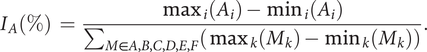 $$ {I}_A\left(\%\right)\hskip0.35em =\hskip0.35em \frac{\max_i\left({A}_i\right)-{\min}_i\left({A}_i\right)}{\sum_{M\in A,B,C,D,E,F}\left({\max}_k\left({M}_k\right)-{\min}_k\left({M}_k\right)\right)}. $$
Expressions are similar for the other factors.
Two models are fitted to the data, one for detection time and one for unpleasantness. An analysis of the parameters of the model is made in order to understand the main effects of the factors on the detectability and the unpleasantness.
Definition of the ‘best’ individual sound
$ {\boldsymbol{IGA}}_{\boldsymbol{opt}}^{\boldsymbol{i}} $

The following method has been set to define a unique QV sound, labelled
 $ {IGA}_{opt}^i $
, for each participant
$ {IGA}_{opt}^i $
, for each participant
 $ i $
. The first stage is to discard solutions of the Pareto set that are too extreme according to one of the objectives. Among the solutions of the individual Pareto set, solutions for which the detection time was above 4.05 seconds were rejected (detection time below the safety zone; see Section 3.3). Similarly, solutions with a very high unpleasantness relative to the unpleasantness range used by the participant were rejected. To do so, a min-max normalisation of the participant’s unpleasantness evaluations was performed, and the sounds in the upper third of the resulting range were withdrawn.
$ i $
. The first stage is to discard solutions of the Pareto set that are too extreme according to one of the objectives. Among the solutions of the individual Pareto set, solutions for which the detection time was above 4.05 seconds were rejected (detection time below the safety zone; see Section 3.3). Similarly, solutions with a very high unpleasantness relative to the unpleasantness range used by the participant were rejected. To do so, a min-max normalisation of the participant’s unpleasantness evaluations was performed, and the sounds in the upper third of the resulting range were withdrawn.
The second stage consists in the definition of a unique sound. With the remaining sounds, for each participant
 $ i $
, the TOPSIS method (Technique for Order of Preference by Similarity to Ideal Solution; Hwang & Yoon Reference Hwang and Yoon1981) was used to select a unique optimal sound,
$ i $
, the TOPSIS method (Technique for Order of Preference by Similarity to Ideal Solution; Hwang & Yoon Reference Hwang and Yoon1981) was used to select a unique optimal sound,
 $ {IGA}_{opt}^i $
. The first step of this method is to build a matrix
$ {IGA}_{opt}^i $
. The first step of this method is to build a matrix
 $ {x}_{kj} $
from the remaining sounds’ objective values, where each row corresponds to a sound
$ {x}_{kj} $
from the remaining sounds’ objective values, where each row corresponds to a sound
 $ k $
and each column corresponds to an objective (in our case,
$ k $
and each column corresponds to an objective (in our case,
 $ j\hskip0.35em =\hskip0.35em 2 $
). Then, each column of
$ j\hskip0.35em =\hskip0.35em 2 $
). Then, each column of
 $ {x}_{kj} $
is normalised by
$ {x}_{kj} $
is normalised by
 $ {\sum}_k{x}_{kj}^2 $
and multiplied by a weight. In our case, we give an equal weight of 0.5 to each objective. Two ideal solutions are then defined:
$ {\sum}_k{x}_{kj}^2 $
and multiplied by a weight. In our case, we give an equal weight of 0.5 to each objective. Two ideal solutions are then defined:
-
(i) the positive ideal solution (PIS) which has, for each objective, the lowest value taken by the solutions in the considered group, meaning that
$ PIS\hskip0.35em =\hskip0.35em \left\{\min \left({x}_{k1}\right),\min \left({x}_{k2}\right)\right\} $
; -
(ii) the negative ideal solution (NIS) which has, for each objective, the highest value taken by the solutions in the considered group, meaning that
$ PIS\hskip0.35em =\hskip0.35em \left\{\max \left({x}_{k1}\right),\max \left({x}_{k2}\right)\right\} $
.


After computing the Euclidean distance between each solution and the PIS and the NIS, respectively, called
 $ {d}_{PIS} $
and
$ {d}_{PIS} $
and
 $ {d}_{NIS} $
, the following distance is computed:
$ {d}_{NIS} $
, the following distance is computed:
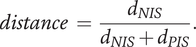 $$ distance\hskip0.35em =\hskip0.35em \frac{d_{NIS}}{d_{NIS}+{d}_{PIS}}. $$
The chosen optimal solution
 $ {IGA}_{opt}^i $
of participant
$ {IGA}_{opt}^i $
of participant
 $ i $
is the one that maximises this distance, which equals 1 if the sounds happen to be the PIS and 0 if it is the NIS.
$ i $
is the one that maximises this distance, which equals 1 if the sounds happen to be the PIS and 0 if it is the NIS.
This process allows the definition of individual optimal sounds
 $ {IGA}_{opt}^i $
, one for each participant
$ {IGA}_{opt}^i $
, one for each participant
 $ i $
.
$ i $
.
Analysis of
$ Optimalset $
, the set of Pareto optimal solutions

The union, for all the participants, of all the individual Pareto solutions is formed. This set, labelled
 $ Optimalset $
, represents a selection of QV sounds that, from a perceptual point of view, make a satisfying trade-off between detectability and unpleasantness for the participants. To provide information that could be used as recommendations for a sound designer, an analysis of these sounds according to the most occurring factor-level combinations is conducted.
$ Optimalset $
, represents a selection of QV sounds that, from a perceptual point of view, make a satisfying trade-off between detectability and unpleasantness for the participants. To provide information that could be used as recommendations for a sound designer, an analysis of these sounds according to the most occurring factor-level combinations is conducted.
To draw design recommendations, the principle of the method is to consider the selection process of the designs made during the IGA experiment as a random process that depends on a discrete probability distribution. The set
 $ Optimalset $
, of size
$ Optimalset $
, of size
 $ N $
, is a subset of the sample space
$ N $
, is a subset of the sample space
 $ \Omega $
(full factorial design). From the chosen designs in
$ \Omega $
(full factorial design). From the chosen designs in
 $ Optimalset $
, estimates of the parameters of the probability distribution can be calculated. And with these parameters, it becomes possible to make inferences and provide a probability score for any design of the design space.
$ Optimalset $
, estimates of the parameters of the probability distribution can be calculated. And with these parameters, it becomes possible to make inferences and provide a probability score for any design of the design space.
Joint probability
Given the sample space
 $ \Omega $
(set of all possible designs of the design space), and the design variables
$ \Omega $
(set of all possible designs of the design space), and the design variables
 $ {X}_i $
, (i = 1–6) that describe the design, the first model that can be made is to assume that the choice of the designs in
$ {X}_i $
, (i = 1–6) that describe the design, the first model that can be made is to assume that the choice of the designs in
 $ Optimalset $
depends on all the variables and all their possible interactions. In this case, the probability distribution of the selection process of any design
$ Optimalset $
depends on all the variables and all their possible interactions. In this case, the probability distribution of the selection process of any design
 $ d $
defined by the design variables
$ d $
defined by the design variables
 $ {X}_i $
, (i = 1–6),
$ {X}_i $
, (i = 1–6),
 $ d\hskip0.35em =\hskip0.35em ({X}_1\hskip0.35em =\hskip0.35em {x}_1,\hskip0.35em {X}_2\hskip0.35em =\hskip0.35em {x}_2,\dots, \hskip0.35em {X}_6\hskip0.35em =\hskip0.35em {x}_6) $
by the IGA experiments is given by the joint probability:
$ d\hskip0.35em =\hskip0.35em ({X}_1\hskip0.35em =\hskip0.35em {x}_1,\hskip0.35em {X}_2\hskip0.35em =\hskip0.35em {x}_2,\dots, \hskip0.35em {X}_6\hskip0.35em =\hskip0.35em {x}_6) $
by the IGA experiments is given by the joint probability:
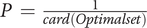
 $$ P\left(D\hskip0.35em =\hskip0.35em d\right)\hskip0.35em =\hskip0.35em P\left({X}_1\hskip0.35em =\hskip0.35em {x}_1,{X}_2\hskip0.35em =\hskip0.35em {x}_2,\dots, {X}_6\hskip0.35em =\hskip0.35em {x}_6\right)\hskip0.35em =\hskip0.35em \frac{\mathit{\operatorname{card}}\left\{D\hskip0.35em \in \hskip0.35em Optimalset/D\hskip0.35em =\hskip0.35em d\right\}}{\mathit{\operatorname{card}}(Optimalset)}, $$
where
 $ \mathit{\operatorname{card}} $
represents the cardinality of a set (number of elements). For example, if a design is present once in
$ \mathit{\operatorname{card}} $
represents the cardinality of a set (number of elements). For example, if a design is present once in
 $ Optimalset $
, its probability is
$ Optimalset $
, its probability is
 $ P\hskip0.35em =\hskip0.35em \frac{1}{\mathit{\operatorname{card}}(Optimalset)} $
.
$ P\hskip0.35em =\hskip0.35em \frac{1}{\mathit{\operatorname{card}}(Optimalset)} $
.
If it is not chosen, its probability is
 $ P\hskip0.35em =\hskip0.35em 0 $
. This six-dimension joint probability is not so interesting to make design recommendations because it is only able to recommend designs that are present (and abundant) in
$ P\hskip0.35em =\hskip0.35em 0 $
. This six-dimension joint probability is not so interesting to make design recommendations because it is only able to recommend designs that are present (and abundant) in
 $ Optimalset $
. To be able to make recommendations on the levels of the design variables
$ Optimalset $
. To be able to make recommendations on the levels of the design variables
 $ {X}_i $
, it is necessary to make assumptions on the independence of the variables in the selection process.
$ {X}_i $
, it is necessary to make assumptions on the independence of the variables in the selection process.
Marginal probability
If we consider that the variables
 $ {X}_i $
(
$ {X}_i $
(
 $ i\hskip0.35em =\hskip0.35em 1 $
–
$ i\hskip0.35em =\hskip0.35em 1 $
–
 $ 6 $
) are mutually independent in the selection process (no interaction between them), then the probability distribution of the selection process of any design
$ 6 $
) are mutually independent in the selection process (no interaction between them), then the probability distribution of the selection process of any design
 $ d\hskip0.35em =\hskip0.35em ({X}_1\hskip0.35em =\hskip0.35em {x}_1,\hskip0.35em {X}_2\hskip0.35em =\hskip0.35em {x}_2,\dots, \hskip0.35em {X}_6\hskip0.35em =\hskip0.35em {x}_6) $
becomes
$ d\hskip0.35em =\hskip0.35em ({X}_1\hskip0.35em =\hskip0.35em {x}_1,\hskip0.35em {X}_2\hskip0.35em =\hskip0.35em {x}_2,\dots, \hskip0.35em {X}_6\hskip0.35em =\hskip0.35em {x}_6) $
becomes
 $$ P\left({X}_1\hskip0.35em =\hskip0.35em {x}_1,{X}_2\hskip0.35em =\hskip0.35em {x}_2,\dots, {X}_6\hskip0.35em =\hskip0.35em {x}_6\right)\hskip0.35em =\hskip0.35em \prod \limits_{i\hskip0.35em =\hskip0.35em 1}^6P\left({X}_i\hskip0.35em =\hskip0.35em {x}_i\right). $$
When the variables are mutually independent, the joint probability is simply the product of the marginal probabilities, where
 $$ P\left({X}_i\hskip0.35em =\hskip0.35em {x}_i\right)\hskip0.35em =\hskip0.35em \frac{\mathit{\operatorname{card}}\left\{D\hskip0.35em \in \hskip0.35em Optimalset/{X}_i\hskip0.35em =\hskip0.35em {x}_i\right\}}{\mathit{\operatorname{card}}(Optimalset)}. $$
In this case, the design with the largest probability, that is, the one that should be recommended, is the design with the most occurring level for each variable. Of course, the mutual independence of all the variables is a very strong assumption that only holds if there is no interaction between the variables in the selection process (in the perception of participants). This is rather unlikely in design where the global assessment of a product may be different to the sum of the assessments of each of its variables (Sylcott, Michalek & Cagan Reference Sylcott, Michalek and Cagan2015).
Independence checking of the variables
Between the two previous methods that have limited applicability for making design recommendations, it is interesting to propose a model that is based on assumptions concerning the independence of the variables in the selection process that can be checked. Our proposal is to check, with a statistical test, the independence of any pairs of variables in
 $ Optimalset $
. We propose to use the chi-square independence test to determine whether there is a significant association between two qualitative variables. For example, suppose that the pairwise independence test shows that the two groups of variables
$ Optimalset $
. We propose to use the chi-square independence test to determine whether there is a significant association between two qualitative variables. For example, suppose that the pairwise independence test shows that the two groups of variables
 $ \left\{{X}_1,{X}_2,{X}_3\right\} $
and
$ \left\{{X}_1,{X}_2,{X}_3\right\} $
and
 $ \left\{{X}_4,{X}_5,{X}_6\right\} $
are independent. Then, from this information, it is possible to simplify the expression of the joint probability and get the probability distribution of the selection process for any design
$ \left\{{X}_4,{X}_5,{X}_6\right\} $
are independent. Then, from this information, it is possible to simplify the expression of the joint probability and get the probability distribution of the selection process for any design
 $ d\hskip0.35em =\hskip0.35em \left({X}_1\hskip0.35em =\hskip0.35em {x}_1,{X}_2\hskip0.35em =\hskip0.35em {x}_2,\dots, {X}_6\hskip0.35em =\hskip0.35em {x}_6\right) $
, given by
$ d\hskip0.35em =\hskip0.35em \left({X}_1\hskip0.35em =\hskip0.35em {x}_1,{X}_2\hskip0.35em =\hskip0.35em {x}_2,\dots, {X}_6\hskip0.35em =\hskip0.35em {x}_6\right) $
, given by
 $$ {\displaystyle \begin{array}{l}P\left({X}_1\hskip0.35em =\hskip0.35em {x}_1,{X}_2\hskip0.35em =\hskip0.35em {x}_2,\dots, {X}_6\hskip0.35em =\hskip0.35em {x}_6\right)\hskip0.35em =\hskip0.35em P\left({X}_1\hskip0.35em =\hskip0.35em {x}_1,{X}_2\hskip0.35em =\hskip0.35em {x}_2,{X}_3\hskip0.35em =\hskip0.35em {x}_3\right)\\ {}\hskip16.24em .P\left({X}_4\hskip0.35em =\hskip0.35em {x}_4,{X}_5\hskip0.35em =\hskip0.35em {x}_5,{X}_6\hskip0.35em =\hskip0.35em {x}_6\right),\end{array}} $$
where
 $$ P\left({X}_1\hskip0.35em =\hskip0.35em {x}_1,{X}_2\hskip0.35em =\hskip0.35em {x}_2,{X}_3\hskip0.35em =\hskip0.35em {x}_3\right)\hskip0.35em =\hskip0.35em \frac{\mathit{\operatorname{card}}\left\{D\hskip0.35em \in \hskip0.35em Optimalset/{X}_1\hskip0.35em =\hskip0.35em {x}_1,{X}_2\hskip0.35em =\hskip0.35em {x}_2,{X}_3\hskip0.35em =\hskip0.35em {x}_3\right\}}{\mathit{\operatorname{card}}(Optimalset)}, $$
 $$ P\left({X}_4\hskip0.35em =\hskip0.35em {x}_4,{X}_5\hskip0.35em =\hskip0.35em {x}_5,{X}_6\hskip0.35em =\hskip0.35em {x}_6\right)\hskip0.35em =\hskip0.35em \frac{\mathit{\operatorname{card}}\left\{D\hskip0.35em \in \hskip0.35em Optimalset/{X}_4\hskip0.35em =\hskip0.35em {x}_4,{X}_5\hskip0.35em =\hskip0.35em {x}_5,{X}_6\hskip0.35em =\hskip0.35em {x}_6\right\}}{\mathit{\operatorname{card}}(Optimalset)}. $$
It is then possible to calculate the probabilities of all the designs
 $ d\hskip0.35em =\hskip0.35em ({X}_1\hskip0.35em =\hskip0.35em {x}_1,\hskip0.35em {X}_2\hskip0.35em =\hskip0.35em {x}_2,\dots, \hskip0.35em {X}_6\hskip0.35em =\hskip0.35em {x}_6) $
of the design space.
$ d\hskip0.35em =\hskip0.35em ({X}_1\hskip0.35em =\hskip0.35em {x}_1,\hskip0.35em {X}_2\hskip0.35em =\hskip0.35em {x}_2,\dots, \hskip0.35em {X}_6\hskip0.35em =\hskip0.35em {x}_6) $
of the design space.
It is important to note that if all the variables are dependent (conjoint graph), the recommendations are simply the list of designs of
 $ Optimalset $
.
$ Optimalset $
.
Recommended designs
A ranking of the design space by decreasing probability allows the definition of the ‘best’ designs, that is, the designs with the largest probabilities, to be recommended. Some of them are of course present in
 $ Optimalset $
, but it is likely that designs that are not present in
$ Optimalset $
, but it is likely that designs that are not present in
 $ Optimalset $
will get a high probability, and be interesting for the design problem. These designs may possess interesting characteristic combinations that explain their presence in the Pareto set. A set of eight sounds (labelled reco1 to reco8) that get the highest probability score is proposed as recommended designs. They will be compared to other designs in Experiment 3.
$ Optimalset $
will get a high probability, and be interesting for the design problem. These designs may possess interesting characteristic combinations that explain their presence in the Pareto set. A set of eight sounds (labelled reco1 to reco8) that get the highest probability score is proposed as recommended designs. They will be compared to other designs in Experiment 3.
Outliers detection procedure
Three indicators were considered to assess the performances of the participants in the detection task for the different experiments:
-
(i) the direction error rate
$ DER $
: percentage of stimuli detected with wrong direction; -
(ii) the early detection rate
$ EDR $
: percentage of stimuli detected before
$ {t}_1 $
; -
(iii) the late detection rate
$ LDR $
: percentage of stimuli detected after
$ {t}_3 $
.


Limit values were defined for the different indicators, by considering the difficulty of the task and possible careless mistakes, inevitable given the relatively high cognitive load required for the experiments. The objective of these limits is not to select the participants, but to discard the dilettantes that did not provide the necessary commitment in the experiment. For these reasons, the limits are relatively large. So that the ratings of a participant are valid, it is necessary to have
 $ DER<40\% $
,
$ DER<40\% $
,
 $ EDR<20\% $
and
$ EDR<20\% $
and
 $ LDR<85\% $
. Otherwise, their data were withdrawn from the study.
$ LDR<85\% $
. Otherwise, their data were withdrawn from the study.
4.2. Results
Outlier detection
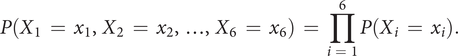
Table 2 shows the average performance indicators (with the standard deviation between brackets) of the participants for the three experiments (Direction error rate
 $ \overline{\mathrm{DER}} $
, early detection rate
$ \overline{\mathrm{DER}} $
, early detection rate
 $ \overline{\mathrm{EDR}} $
and late detection rate
$ \overline{\mathrm{EDR}} $
and late detection rate
 $ \overline{\mathrm{LDR}} $
). For Experiment 1, these average indicators show acceptable performances of the participants, indicating that the protocol is correctly designed and does not require outstanding abilities from the participants. The direction error rate (7.1%) remained weak and can be explained by haste mistakes of the participants. One participant made many wrong direction detections (above 40%), which is interpreted as a sign of an inability to use the interface correctly. This is probably due to some misunderstandings of the instructions. For those reasons, the data from this participant (several standard deviations away from the average) were not considered for the analysis. The early detection rate was very low (0.4%), which is a sign that the participants waited for the car and did not rush the test. The large average late detection rate (17.6%) indicates that some sounds are particularly hard to detect for some participants. Three participants had very high late detection rate (above 85% – due probably to a weak involvement in the experiment). For this reason, their data (several standard deviations away from the average) were excluded from the analysis. In summary, four participants among the 32 were withdrawn from the analysis due to low performance rates in their detection, leading to 28 valid participants.
$ \overline{\mathrm{LDR}} $
). For Experiment 1, these average indicators show acceptable performances of the participants, indicating that the protocol is correctly designed and does not require outstanding abilities from the participants. The direction error rate (7.1%) remained weak and can be explained by haste mistakes of the participants. One participant made many wrong direction detections (above 40%), which is interpreted as a sign of an inability to use the interface correctly. This is probably due to some misunderstandings of the instructions. For those reasons, the data from this participant (several standard deviations away from the average) were not considered for the analysis. The early detection rate was very low (0.4%), which is a sign that the participants waited for the car and did not rush the test. The large average late detection rate (17.6%) indicates that some sounds are particularly hard to detect for some participants. Three participants had very high late detection rate (above 85% – due probably to a weak involvement in the experiment). For this reason, their data (several standard deviations away from the average) were excluded from the analysis. In summary, four participants among the 32 were withdrawn from the analysis due to low performance rates in their detection, leading to 28 valid participants.
Average participants performance rates and number of participants
 $ n $
not meeting the control limits, for the three experiments. Standard deviations (SD) of the rates are indicated between brackets.
$ n $
not meeting the control limits, for the three experiments. Standard deviations (SD) of the rates are indicated between brackets.
Convergence of IGA
The sum of the two objectives was examined in order to show the convergence of the solutions across the different generations. Before summing, the value of the detection time was scaled so that its range matched the one of the unpleasantness. Please note that the IGA do not directly operate on this sum as it is a multiobjective optimisation. That being said, we believe that this reduction to a single objective is a convenient way to monitor the behaviour of the IGA.
Figure 8 shows the sum averaged over all participants plotted for two conditions: the mean value for the solutions of a generation and the minimum value for a generation. On average, the objectives’ sum is decreasing over the generations, which shows an improvement of the proposed sounds with regard to the design problem. This is a sign of the reliability of the experimental protocol for the assessment of the detection time and the unpleasantness, and a correct tuning of the IGA parameters.
Average value of the sum of the two objectives versus generations, with the standard error. The value of the detection time has been scaled so that its range matches the one of the unpleasantness.
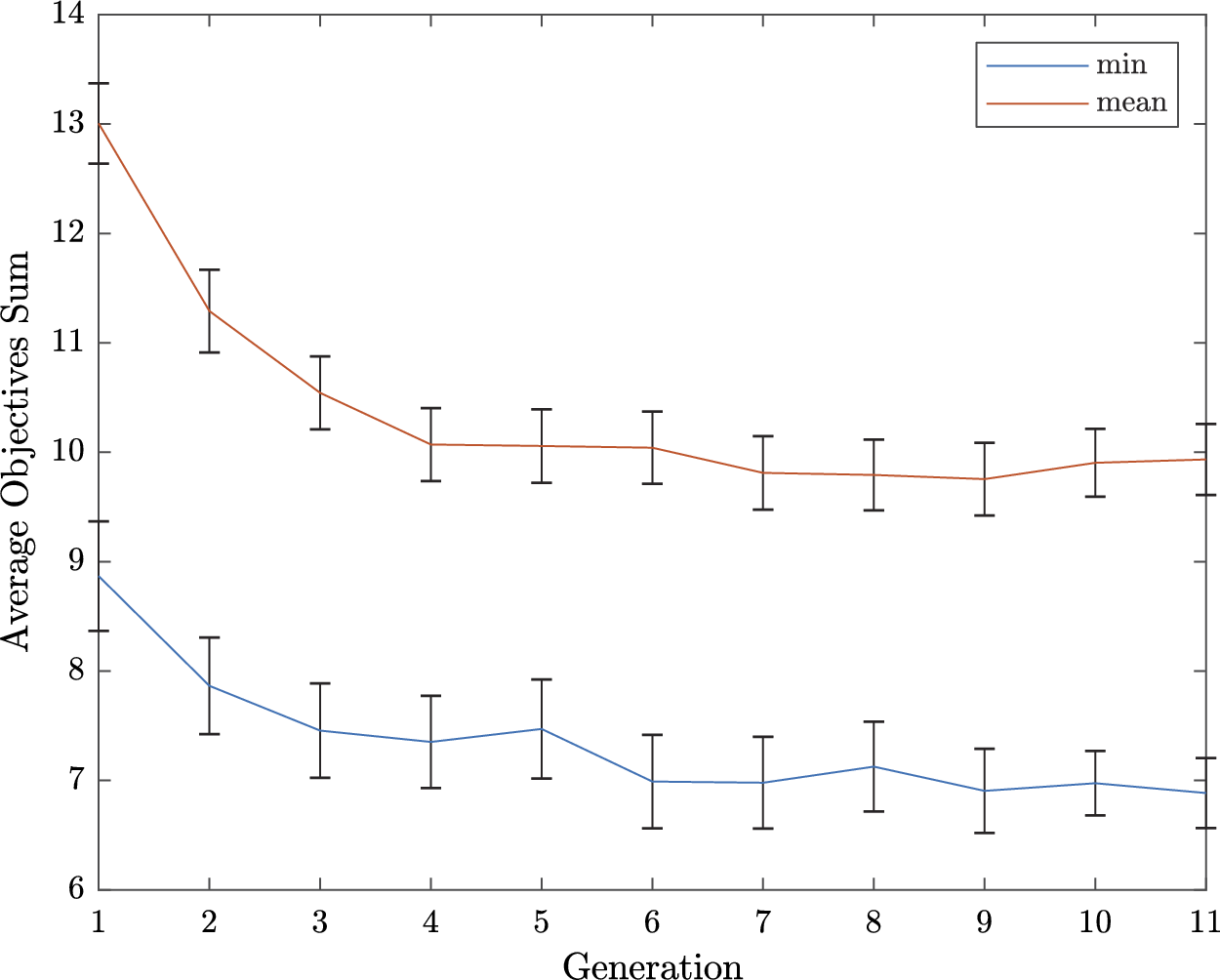
Analysis of the effect of the factors
The results of the two linear models between the sound characteristics (detectability and unpleasantness) and the six design factors are given in Table 3. All the assessments made by the valid participants (28 × 99 = 2772 observations) during the IGA experiments are used for the modelling. For the two models, the determination coefficient
 $ {R}^2 $
is not large (43% and 46%), indicating that the models are approximate and gather only a general trend in the data. They thus cannot be used to make accurate predictions of the responses (recommendations). Nevertheless, all the factors are significant in the model (p < 0.001), and they are therefore useful to explain the variability in the two responses. The importance of the factors is rather similar (around 100/6 = 16.6%), except Factor E (amplitude modulation frequency), which has a weaker influence on detectability (7.1%) and unpleasantness (6.4%), and Factor B (fundamental/centre frequency), which has a larger influence (34.3% and 27.2%).
$ {R}^2 $
is not large (43% and 46%), indicating that the models are approximate and gather only a general trend in the data. They thus cannot be used to make accurate predictions of the responses (recommendations). Nevertheless, all the factors are significant in the model (p < 0.001), and they are therefore useful to explain the variability in the two responses. The importance of the factors is rather similar (around 100/6 = 16.6%), except Factor E (amplitude modulation frequency), which has a weaker influence on detectability (7.1%) and unpleasantness (6.4%), and Factor B (fundamental/centre frequency), which has a larger influence (34.3% and 27.2%).
Coefficients, p-value of the significance Fisher test and importance of the factor for the two linear models (unpleasantness and detectability)
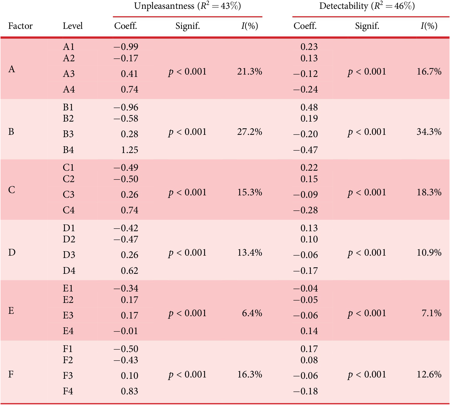
The values of the coefficients of the models (graph of the main effects) are presented in Figure 9 for unpleasantness and detectability. From these graphs, it is clear that there is an opposition between detectability and unpleasantness: the general trend is that to have a ‘pleasant’ sound, the levels of all the factors must be low (Level 1), and to have a detectable sound, the levels of all the factors must be high (Level 4). The lower the level’s modality, the more pleasant the sounds, and the higher the level’s modality, the more detectable the sounds. Factor E has a little more complex effect for Level 4 (Level 4 is not the most unpleasant and the most detectable). This analysis confirms the trade-off between detectability and unpleasantness that is mentioned in other studies (Parizet et al. Reference Parizet, Robart, Chamard, Schlittenlacher, Pondrom, Ellermeier, Biancardi, Janssens, Speed-Andrews, Cockram and Hatton2013; Lee et al. Reference Lee, Lee, Shin and Han2017). Furthermore, an examination of the values of the different levels shows that the results are in accordance with previous studies: to be ‘not unpleasant’, the sound must resemble an ICE sound (A1), be low pitched (B1 – low frequency), be made of noise (C1 – no harmonic sound; see the whine index in Lee et al. Reference Lee, Lee, Shin and Han2017) and with no modulation (F1); to be detectable, the sound must be high pitched (B4 – high frequency), with an harmonic content (A4, C4) and with modulation (F4).
Graph of the coefficients of the linear mixed models of unpleasantness and detectability for the six factors A, B, C, D, E and F.
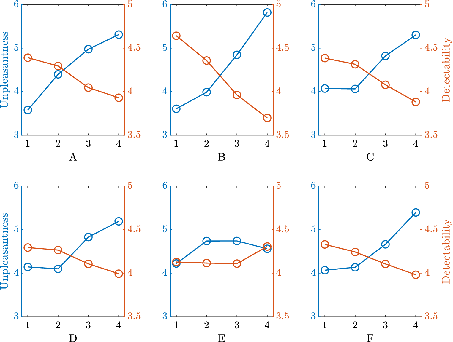
However, this opposition between detectability and unpleasantness is only a general trend, revealed by a linear model that account for less than 50% of variance. Particular QV sounds with adapted combinations of factor levels may optimise at the same time detectability and unpleasantness, but this approximate model does not provide us with enough information to find these trade-off sounds. This motivates the need for an alternative method for making recommendations.
Analysis of the sounds of
$ Optimalset $

One variable at once
The
 $ Optimalset $
(union of the Pareto front of all the participants) counts N = 113 sounds. All of them are Pareto optimal, representing different compromises between unpleasantness and detectability. For each participant, the Pareto front of the best-solution register contained 1–8 solutions. All designs are present once, except d1(A1 B4 C4 D4 E2 F1) present twice and d2(A2 B4 C4 D4 E1 F1) present four times. The occurrences of the levels of each factor in
$ Optimalset $
(union of the Pareto front of all the participants) counts N = 113 sounds. All of them are Pareto optimal, representing different compromises between unpleasantness and detectability. For each participant, the Pareto front of the best-solution register contained 1–8 solutions. All designs are present once, except d1(A1 B4 C4 D4 E2 F1) present twice and d2(A2 B4 C4 D4 E1 F1) present four times. The occurrences of the levels of each factor in
 $ Optimalset $
are given in Table 4.
$ Optimalset $
are given in Table 4.
Occurrences of the levels of each factor in
 $ Optimalset $
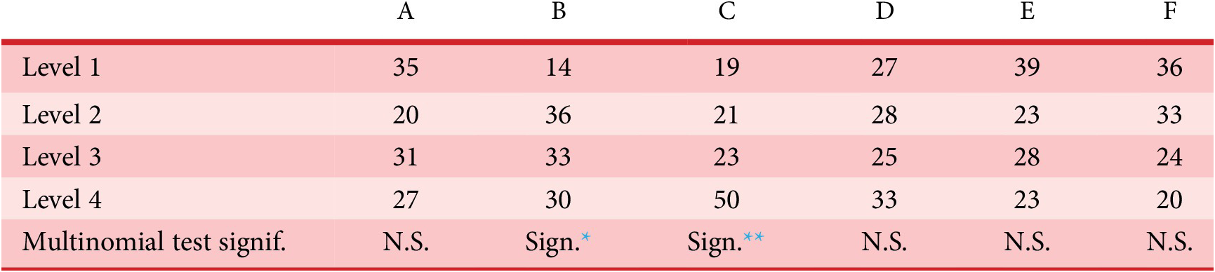
Abbreviation: N.S.: not significant.
*
 $ p<0.05 $
**
 $ p<0.01 $
For example, for the Harmonic/noise proportion (C), the level C4 (no noise) is chosen 50 times. To define the variables subjected to the most consensual choice concerning their levels, a multinomial goodness-of-fit test of the distribution of the occurrences is carried out. Results are presented in Table 4. Only two factors (B [frequency] and C [Harmonic/noise proportion]) obtain occurrences significantly different from a random distribution at the 5% level. For the frequency of the sounds, the level B1 (low frequency) is under-represented (size = 14). For the Harmonic/noise proportion, the level C4 (broad band noise absent) is over-represented (size = 50). For the whole group of participants, according to a majority compromise, it seems necessary to avoid low frequencies and broadband noise for the high detectability and low unpleasantness of QV sounds. For the other variables, it is not possible to make recommendations with this simple sorting one variable at once, either because there are groups of subjects with different views on these variables, or because there is no clear influence of each variable alone on the compromise (interactions). These results are in line with the models proposed in the previous section. Given that the two objectives are conflicting for all the variables, there is no obvious optimum when one considers each variable alone.
Independence test of the factors in Optimalset
With the definition of the N designs of
 $ Optimalset $
, contingency tables of all pairs of variables are formed. The results of the chi-square test of independence (p-value) are given in Table 5. The p-values corresponding to a rejection of the independence are presented in bold (a Bonferroni correction is applied to deal with the multiple comparisons problem – threshold value of
$ Optimalset $
, contingency tables of all pairs of variables are formed. The results of the chi-square test of independence (p-value) are given in Table 5. The p-values corresponding to a rejection of the independence are presented in bold (a Bonferroni correction is applied to deal with the multiple comparisons problem – threshold value of
 $ 0.05/15\hskip0.35em =\hskip0.35em 0.003 $
, where 15 is the number of pairs). For the nonsignificant pairs, the test shows that the dependence in the sample is too weak to distinguish it from independence. From this table, the corresponding dependence graph can be drawn (Figure 10).
$ 0.05/15\hskip0.35em =\hskip0.35em 0.003 $
, where 15 is the number of pairs). For the nonsignificant pairs, the test shows that the dependence in the sample is too weak to distinguish it from independence. From this table, the corresponding dependence graph can be drawn (Figure 10).
Graph of the dependency between the factors.

Pairwise comparison matrix of the chi-square test of independence (p-value)
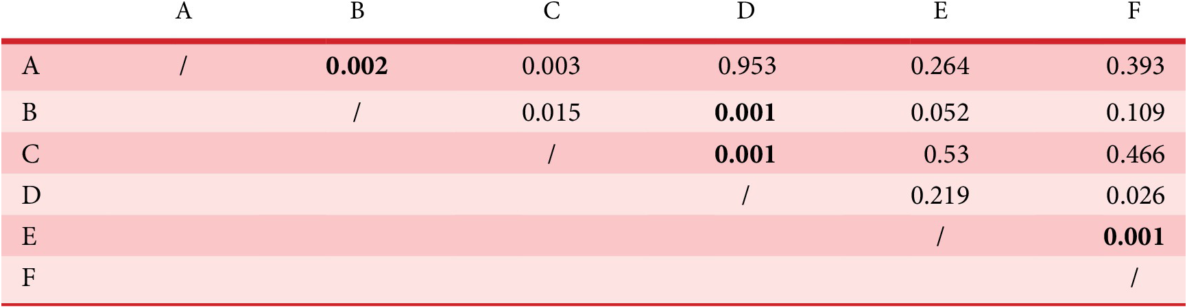
The graph shows that two groups of mutually independent variables can be considered in
 $ Optimalset $
:
$ Optimalset $
:
 $ \left\{A,B,C,D\right\} $
and
$ \left\{A,B,C,D\right\} $
and
 $ \left\{E,F\right\} $
. These indicate that there might be some interaction effect between Factors A, B, C and D on the performance of a sound, when considering both objectives. Likewise for Factors E and F. In other words, it signifies that it is not possible to make recommendations for the level of a single variable in the sets
$ \left\{E,F\right\} $
. These indicate that there might be some interaction effect between Factors A, B, C and D on the performance of a sound, when considering both objectives. Likewise for Factors E and F. In other words, it signifies that it is not possible to make recommendations for the level of a single variable in the sets
 $ \left\{A,B,C,D\right\} $
or
$ \left\{A,B,C,D\right\} $
or
 $ \left\{E,F\right\} $
. All the variables in the set must be considered. The empirical probability law of the selection process is then given by
$ \left\{E,F\right\} $
. All the variables in the set must be considered. The empirical probability law of the selection process is then given by
 $$ {\displaystyle \begin{array}{l}P(A\hskip0.35em =\hskip0.35em {A}_i,\hskip0.35em B\hskip0.35em =\hskip0.35em {B}_j,\hskip0.35em C\hskip0.35em =\hskip0.35em {C}_k,\hskip0.35em D\hskip0.35em =\hskip0.35em {D}_l,\hskip0.35em E\hskip0.35em =\hskip0.35em {E}_m,\hskip0.35em F\hskip0.35em =\hskip0.35em {F}_n)\approx \\ {}\hskip7em P(A\hskip0.35em =\hskip0.35em {A}_i,\hskip0.35em B\hskip0.35em =\hskip0.35em {B}_j,\hskip0.35em C\hskip0.35em =\hskip0.35em {C}_k,\hskip0.35em D\hskip0.35em =\hskip0.35em {D}_l).\hskip0.35em P(E\hskip0.35em =\hskip0.35em {E}_m,\hskip0.35em F\hskip0.35em =\hskip0.35em {F}_n).\end{array}} $$
From this expression, the probability scores of all the design samples of the full factorial can be calculated, based on the probability score of each group of variables.
 $ P(A\hskip0.35em =\hskip0.35em {A}_i,\hskip0.35em B\hskip0.35em =\hskip0.35em {B}_j,\hskip0.35em C\hskip0.35em =\hskip0.35em {C}_k,\hskip0.35em D\hskip0.35em =\hskip0.35em {D}_l) $
is computed as the number of designs in
$ P(A\hskip0.35em =\hskip0.35em {A}_i,\hskip0.35em B\hskip0.35em =\hskip0.35em {B}_j,\hskip0.35em C\hskip0.35em =\hskip0.35em {C}_k,\hskip0.35em D\hskip0.35em =\hskip0.35em {D}_l) $
is computed as the number of designs in
 $ Optimalset $
for which
$ Optimalset $
for which
 $ A\hskip0.35em =\hskip0.35em {A}_i $
,
$ A\hskip0.35em =\hskip0.35em {A}_i $
,
 $ B\hskip0.35em =\hskip0.35em {B}_j $
,
$ B\hskip0.35em =\hskip0.35em {B}_j $
,
 $ C\hskip0.35em =\hskip0.35em {C}_k $
and
$ C\hskip0.35em =\hskip0.35em {C}_k $
and
 $ D\hskip0.35em =\hskip0.35em {D}_l $
, divided by the number of designs in
$ D\hskip0.35em =\hskip0.35em {D}_l $
, divided by the number of designs in
 $ Optimalset $
. Likewise for
$ Optimalset $
. Likewise for
 $ P\left(E\hskip0.35em =\hskip0.35em {E}_m,F\hskip0.35em =\hskip0.35em {F}_n\right) $
. Designs with the largest probability (see Table 6) can be recommended as their factor-level combinations constitute attractive characteristics for the Pareto set. They are considered as relevant design solutions to the problem. Because the score contributions from the variable groups
$ P\left(E\hskip0.35em =\hskip0.35em {E}_m,F\hskip0.35em =\hskip0.35em {F}_n\right) $
. Designs with the largest probability (see Table 6) can be recommended as their factor-level combinations constitute attractive characteristics for the Pareto set. They are considered as relevant design solutions to the problem. Because the score contributions from the variable groups
 $ \left\{A,B,C,D\right\} $
and
$ \left\{A,B,C,D\right\} $
and
 $ \left\{E,F\right\} $
are computed independently, some designs might have a high score even though they are not in
$ \left\{E,F\right\} $
are computed independently, some designs might have a high score even though they are not in
 $ Optimalset $
.
$ Optimalset $
.
For the remainder of the paper, the independence between
 $ \left\{A,B,C,D\right\} $
and
$ \left\{A,B,C,D\right\} $
and
 $ \left\{E,F\right\} $
will be indicated by a vertical separator in design descriptions (e.g., [A1 B4 C4 D4
$ \left\{E,F\right\} $
will be indicated by a vertical separator in design descriptions (e.g., [A1 B4 C4 D4
 $ \mid $
E2 F1] for
$ \mid $
E2 F1] for
 $ design1 $
).
$ design1 $
).
Definition of the eight recommended designs (design variables’ levels). The dashed line highlights the independence between
 $ \left\{A,B,C,D\right\} $
and
$ \left\{A,B,C,D\right\} $
and
 $ \left\{E,F\right\} $
.
$ \left\{E,F\right\} $
.
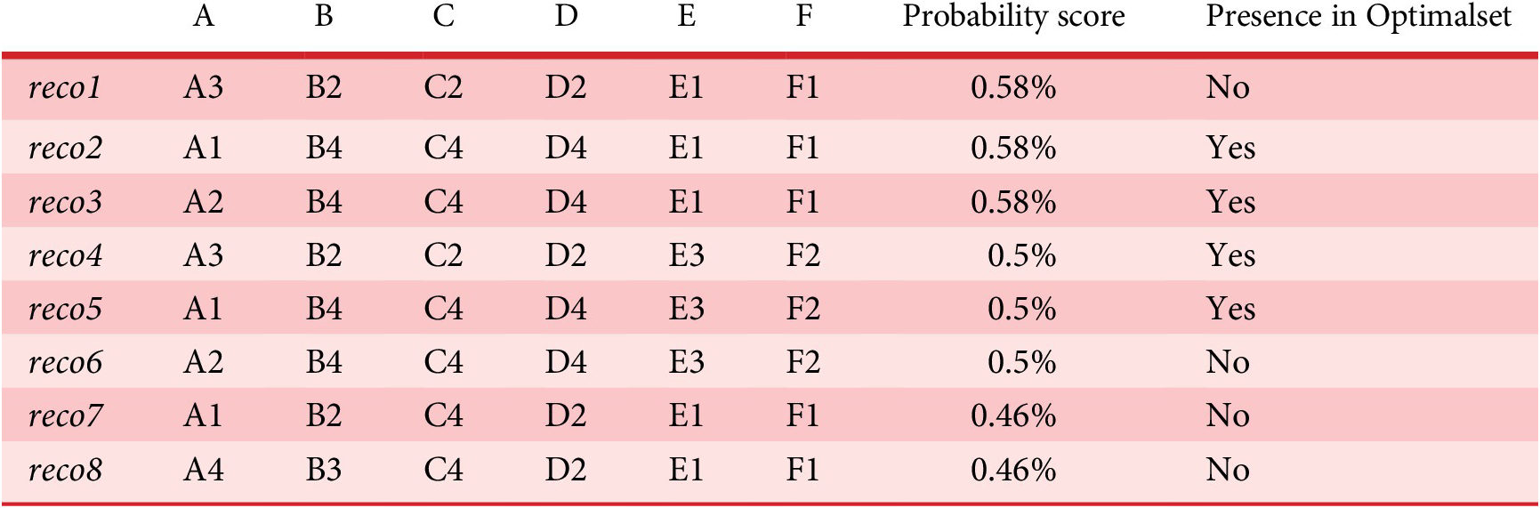
Design recommendations
The eight designs with the largest probability scores (reco1 to reco8 – ranked by decreasing probability) are presented in Table 6. Half of them are presented in
 $ Optimalset $
. They present combinations of variables that may be interesting for the design problem. It is interesting to mention that different levels of the factors are present in the recommended designs: no single level presents a paramount advantage for the design problem. It is instead the combination of different levels that constitute an interesting sound. This is in agreement with the results of the models of unpleasantness and detectability, which showed that no recommendation can be made independently on each factor because of the conflicting objectives.
$ Optimalset $
. They present combinations of variables that may be interesting for the design problem. It is interesting to mention that different levels of the factors are present in the recommended designs: no single level presents a paramount advantage for the design problem. It is instead the combination of different levels that constitute an interesting sound. This is in agreement with the results of the models of unpleasantness and detectability, which showed that no recommendation can be made independently on each factor because of the conflicting objectives.
5. Experiment 2: individual validation
5.1. Materials and method
One week after Experiment 1 (time to analyse the results), the second experiment was proposed to the participants of Experiment 1. Twenty-four out of the 32 previous subjects re-evaluated their own optimal solution
 $ {IGA}_{opt}^i $
, as well as two designed sounds (
$ {IGA}_{opt}^i $
, as well as two designed sounds (
 $ design1 $
and
$ design1 $
and
 $ design2 $
) and four random sounds (
$ design2 $
) and four random sounds (
 $ rand1 $
,
$ rand1 $
,
 $ rand2 $
,
$ rand2 $
,
 $ rand3 $
and
$ rand3 $
and
 $ rand4 $
).
$ rand4 $
).
The designed sounds were proposed by a skilled person having a thorough knowledge of the possibilities offered by the synthesiser (T.S., one of the co-authors). These designs were intended to be good compromises between unpleasantness and detection time while having a different timbre with respect to one another. They were designed by tuning the parameters of the synthesiser while listening to its output, without prior information on the preferences of the test group. This allowed the designer to develop an intuition of how the design parameters related to his own perception of unpleasantness and detectability. The designer tried to find areas of the design space where a small change in parameters would make the sound either too unpleasant or not detectable enough. The sound
 $ design1 $
is high pitched, with a small number of harmonics, no noise content and no amplitude modulation. Its parameter values are (A2 B4 C4 D2
$ design1 $
is high pitched, with a small number of harmonics, no noise content and no amplitude modulation. Its parameter values are (A2 B4 C4 D2
 $ \mid $
E1 F1). The sound
$ \mid $
E1 F1). The sound
 $ design2 $
is pitched slightly lower, with just noise and fast, low amplitude modulation. Its parameter values are (A1 B3 C1 D1
$ design2 $
is pitched slightly lower, with just noise and fast, low amplitude modulation. Its parameter values are (A1 B3 C1 D1
 $ \mid $
E4 F2).
$ \mid $
E4 F2).
In addition to these two designed sounds, four random sounds (
 $ rand1 $
,
$ rand1 $
,
 $ rand2 $
,
$ rand2 $
,
 $ rand3 $
and
$ rand3 $
and
 $ rand4 $
) are generated by a random generation in the design space based on a Latin Hypercube Sampling. Those sounds are taken as baseline to judge the relative performances of the other sounds, designed and
$ rand4 $
) are generated by a random generation in the design space based on a Latin Hypercube Sampling. Those sounds are taken as baseline to judge the relative performances of the other sounds, designed and
 $ IGA $
. The sounds can be listened to at https://mathieulagrange.github.io/souaille2021interactive/.
$ IGA $
. The sounds can be listened to at https://mathieulagrange.github.io/souaille2021interactive/.
All subjects evaluated the same designed and random sounds, together with their own optimum
 $ {IGA}_{opt}^i $
. All the assessments were repeated four times to stabilise variance. Thus, each participant had to evaluate 7 × 4 = 28 sounds, presented one at a time (one per page in the interface), in a random order. For each evaluation, the interface was identical and there was no indication regarding which sound is being evaluated.
$ {IGA}_{opt}^i $
. All the assessments were repeated four times to stabilise variance. Thus, each participant had to evaluate 7 × 4 = 28 sounds, presented one at a time (one per page in the interface), in a random order. For each evaluation, the interface was identical and there was no indication regarding which sound is being evaluated.
First, in order to assess the ability of subjects to perceive differences (intra-individual variability compared to inter-sounds variability), a one-way ANOVA (with the factor type of sounds) was done for each subject and each objective (omnibus test).
The sounds were next compared using two criteria:
-
(i) Their membership to the Pareto front, based on their mean unpleasantness and detection time. This does not include any statistical test.
-
(ii) The statistical significance of the pairwise differences between the mean unpleasantness values, for all pairs of sounds. Likewise for the detection time. Tukey’s HSD (Honestly Significant Difference) test was used to assess these differences for each pair of sounds among
$ {IGA}_{opt}^i $
,
$ design1 $
,
$ design2 $
,
$ rand1 $
,
$ rand2 $
,
$ rand3 $
and
$ rand4 $
.


5.2. Results
As illustrated in Table 2, there was no outlier for this experiment. Therefore, all the participants were considered as valid.
The ANOVA performed on each subject’s unpleasantness and detectability ratings showed a significant effect (
 $ p<0.05 $
) of the sound on unpleasantness, for all but two subjects. Almost all the subjects were able to overall discriminate the sounds. For detectability, a significant effect was found for only 8 out of the 24 subjects. The discrimination was then weaker for detectability. We believe that this is because the detectability differences between the sounds of Experiment 2 were too close, for certain subjects, to their just noticeable difference.
$ p<0.05 $
) of the sound on unpleasantness, for all but two subjects. Almost all the subjects were able to overall discriminate the sounds. For detectability, a significant effect was found for only 8 out of the 24 subjects. The discrimination was then weaker for detectability. We believe that this is because the detectability differences between the sounds of Experiment 2 were too close, for certain subjects, to their just noticeable difference.
The mean evaluations of detection time and unpleasantness for all the participants and all the repetitions are computed for the following sounds:
 $ {IGA}_{opt}^i $
,
$ {IGA}_{opt}^i $
,
 $ design1 $
,
$ design1 $
,
 $ design2 $
,
$ design2 $
,
 $ rand2 $
,
$ rand2 $
,
 $ rand2 $
,
$ rand2 $
,
 $ rand3 $
and
$ rand3 $
and
 $ rand4 $
. The average scores and their standard error are presented in Figure 11 for unpleasantness and Figure 12 for detection time. Results of Tukey’s HSD multiple comparison tests are also presented in these figures (significant threshold: p = 0.05): results are presented with bold lines connecting the sounds. When sounds are connected, pairs are not significantly different, whereas they are when not connected.
$ rand4 $
. The average scores and their standard error are presented in Figure 11 for unpleasantness and Figure 12 for detection time. Results of Tukey’s HSD multiple comparison tests are also presented in these figures (significant threshold: p = 0.05): results are presented with bold lines connecting the sounds. When sounds are connected, pairs are not significantly different, whereas they are when not connected.
Experiment 2: average unpleasantness and results of the post hoc analysis for the different quiet vehicle sounds. The black horizontal lines show groups means that are not significantly different (Tukey’s HSD test [
 $ p>0.05 $
]).
$ p>0.05 $
]).
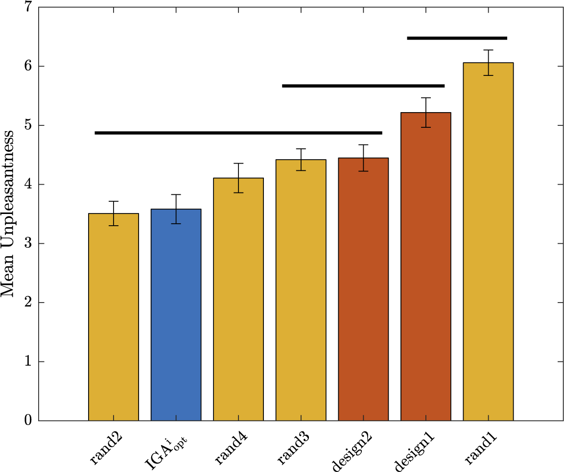
Experiment 2: average detection time and results of the post hoc analysis for the different quiet vehicle sounds. The black horizontal lines show groups means that are not significantly different (Tukey’s HSD test [
 $ p>0.05 $
]).
$ p>0.05 $
]).
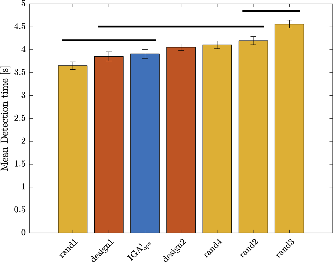
According to unpleasantness (Figure 11), the sound
 $ {IGA}_{opt}^i $
is the second least unpleasant. There is no significant difference within three groups of sounds: (
$ {IGA}_{opt}^i $
is the second least unpleasant. There is no significant difference within three groups of sounds: (
 $ rand2 $
,
$ rand2 $
,
 $ {IGA}_{opt}^i $
,
$ {IGA}_{opt}^i $
,
 $ rand4 $
,
$ rand4 $
,
 $ rand3 $
,
$ rand3 $
,
 $ design2 $
), (
$ design2 $
), (
 $ rand3 $
,
$ rand3 $
,
 $ design2 $
,
$ design2 $
,
 $ design1 $
) and (
$ design1 $
) and (
 $ design1 $
,
$ design1 $
,
 $ rand1 $
). Even if
$ rand1 $
). Even if
 $ {IGA}_{opt}^i $
is not significantly less unpleasant than all the other proposals (particularly the sound
$ {IGA}_{opt}^i $
is not significantly less unpleasant than all the other proposals (particularly the sound
 $ \mathit{\operatorname{rand}}2 $
that is judged as the least unpleasant), it is among the least unpleasant sounds. In particular, it is significantly less unpleasant than the sound
$ \mathit{\operatorname{rand}}2 $
that is judged as the least unpleasant), it is among the least unpleasant sounds. In particular, it is significantly less unpleasant than the sound
 $ design1 $
.
$ design1 $
.
According to detection time (Figure 12), the sound
 $ {IGA}_{opt}^i $
is the third most detectable sound. There is no significant difference within three groups of sounds: (
$ {IGA}_{opt}^i $
is the third most detectable sound. There is no significant difference within three groups of sounds: (
 $ rand1 $
,
$ rand1 $
,
 $ design1 $
,
$ design1 $
,
 $ {IGA}_{opt}^i $
), (
$ {IGA}_{opt}^i $
), (
 $ design1 $
,
$ design1 $
,
 $ {IGA}_{opt}^i $
,
$ {IGA}_{opt}^i $
,
 $ design2 $
,
$ design2 $
,
 $ rand4 $
,
$ rand4 $
,
 $ rand2 $
) and (
$ rand2 $
) and (
 $ rand2 $
,
$ rand2 $
,
 $ rand3 $
). Again,
$ rand3 $
). Again,
 $ {IGA}_{opt}^i $
is not significantly more detectable than all the other proposals, but it belongs to the three most detectable sounds. In particular, it is as detectable as the two designed sounds
$ {IGA}_{opt}^i $
is not significantly more detectable than all the other proposals, but it belongs to the three most detectable sounds. In particular, it is as detectable as the two designed sounds
 $ design1 $
and
$ design1 $
and
 $ design2 $
(no significant difference).
$ design2 $
(no significant difference).
If we consider a stopping distance of 7.5 m at 20 km/hour, the detection time has to be below 4.05 seconds in order to avoid collision. This means that the sounds
 $ rand4 $
,
$ rand4 $
,
 $ rand2 $
and
$ rand2 $
and
 $ rand3 $
do not allow the QV to stay in a safety zone with regard to detectability for blind people. The sound
$ rand3 $
do not allow the QV to stay in a safety zone with regard to detectability for blind people. The sound
 $ {IGA}_{opt}^i $
is in the safety zone, whereas the sound
$ {IGA}_{opt}^i $
is in the safety zone, whereas the sound
 $ design2 $
is close to the limit.
$ design2 $
is close to the limit.
To examine the efficiency of the sounds according to the two objectives together, Figure 13 presents the positions of the sounds in the plane of the two objectives, with the corresponding standard errors. The results show that the individual sound of each participant
 $ {IGA}_{opt}^i $
makes on average an excellent compromise between the two objectives. Even if the sound
$ {IGA}_{opt}^i $
makes on average an excellent compromise between the two objectives. Even if the sound
 $ {IGA}_{opt}^i $
does not Pareto dominate all the other sounds, it belongs to the Pareto front, with the sounds
$ {IGA}_{opt}^i $
does not Pareto dominate all the other sounds, it belongs to the Pareto front, with the sounds
 $ rand2 $
,
$ rand2 $
,
 $ design1 $
and
$ design1 $
and
 $ rand1 $
. The sound
$ rand1 $
. The sound
 $ rand2 $
is not unpleasant, but the price to pay is a large detection time (beyond the safety zone). Conversely,
$ rand2 $
is not unpleasant, but the price to pay is a large detection time (beyond the safety zone). Conversely,
 $ rand1 $
is very detectable, but the most unpleasant.
$ rand1 $
is very detectable, but the most unpleasant.
 $ {IGA}_{opt}^i $
Pareto dominates the sound
$ {IGA}_{opt}^i $
Pareto dominates the sound
 $ design2 $
, whereas it can be considered as equivalent (the same rank) to the sound
$ design2 $
, whereas it can be considered as equivalent (the same rank) to the sound
 $ design1 $
. In conclusion,
$ design1 $
. In conclusion,
 $ {IGA}_{opt}^i $
constitutes an interesting trade-off between the two objectives, as well as the sound
$ {IGA}_{opt}^i $
constitutes an interesting trade-off between the two objectives, as well as the sound
 $ design1 $
. The
$ design1 $
. The
 $ random $
sounds are either Pareto dominated by
$ random $
sounds are either Pareto dominated by
 $ {IGA}_{opt}^i $
, or too extreme on one of the objectives to constitute relevant proposals.
$ {IGA}_{opt}^i $
, or too extreme on one of the objectives to constitute relevant proposals.
Experiment 2: scatterplot of the average performances of the different quiet vehicle sound categories (IGA, Designed, Random) according to the two objectives: unpleasantness and detection time. The dashed line indicates the Pareto front.
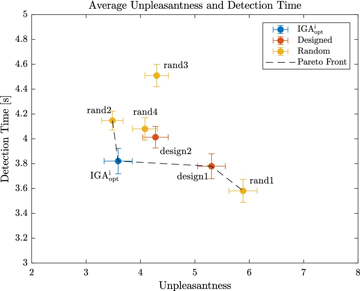
This result validates the efficiency of the IGA experiment for the design of sounds, at least at the individual level. We can then give a positive response to question Q1: Sounds designed with the IGA experiment and selected with the TOPSIS method are interesting candidates for the design problem, comparable in terms of efficiency to sounds designed by a designer.
6. Experiment 3: validation of the recommendation method
6.1. Materials and method
In this experiment, a second panel of subjects (different from the previous panel) is asked to assess the detectability and unpleasantness of different QV sound proposals, including the recommended designs obtained with the method described previously (see the ‘Recommended designs’ and ‘Design recommendations’ sections). Seventeen students (14 males and 3 females) from the École Centrale de Nantes, France, with no reported auditory deficiencies, participated to the test with the protocol described previously. Eighteen QV sounds were proposed to the evaluation:
-
(i) Eight sounds (
$ rand1 $
to
$ rand8 $
– category
$ Random $
) randomly defined in the experimental space.
$ rand1 $
to
$ rand4 $
are the same random sound as in Experiment 2. -
(ii) Two sounds (
$ design1 $
and
$ design2 $
– category
$ Designed $
), designed by a sound designer with instructions for ‘good detectability’ and ‘low unpleasantness’. These sounds are the same as those of Experiment 2. -
(iii) Eight sounds (
$ reco1 $
to
$ reco8 $
– category
$ Recommended $
), recommended by the method described in the previous section (sounds with the largest probability according to the selection process).


To be able to assess the experimental variability in the assessments, four repetitions of each sound were proposed. In total, each participant had to assess 72 (18 × 4) QV sounds, proposed in a randomised order. The performances of each pair of sounds were compared using Tukey’s HSD Multiple Comparison test. Just like for Experiment 2, the intra-individual variability was assessed with two ANOVAs for each subject, one for unpleasantness and one for detection time.
The sounds were compared using the same two criteria as for Experiment 2 (Membership to the Pareto front and multiple comparison tests).
6.2. Results
Outlier detection
As indicated in Table 2, there was no outlier for this experiment. Therefore, all the participants were considered as valid.
Intra-subject variability
The one-way ANOVA performed on the subject’s unpleasantness and detectability ratings showed a significant effect of the sound (
 $ p<0.05 $
) for all but one subject in the case of the unpleasantness and all but another subject in the case of detectability. Almost all the subjects were then able to perceive significant differences between the sounds (omnibus test).
$ p<0.05 $
) for all but one subject in the case of the unpleasantness and all but another subject in the case of detectability. Almost all the subjects were then able to perceive significant differences between the sounds (omnibus test).
Multiple comparisons
From the assessments of the participants according to detectability and unpleasantness, the average scores of detectability and unpleasantness of the 18 QV sounds were calculated. The average scores and their standard errors are presented in Figure 14 for unpleasantness and Figure 15 for detection time together with the Tukey’s HSD multiple comparison test for every pair of sounds (significant threshold:
 $ p\hskip0.35em =\hskip0.35em 0.05 $
).
$ p\hskip0.35em =\hskip0.35em 0.05 $
).
Experiment 3: bar graph of the average value of the unpleasantness for the different quiet vehicle sounds. Nonsignificant differences between pairs of sounds (
 $ p>0.05 $
) are linked with a horizontal line (Tukey’s HSD multiple comparisons test).
$ p>0.05 $
) are linked with a horizontal line (Tukey’s HSD multiple comparisons test).
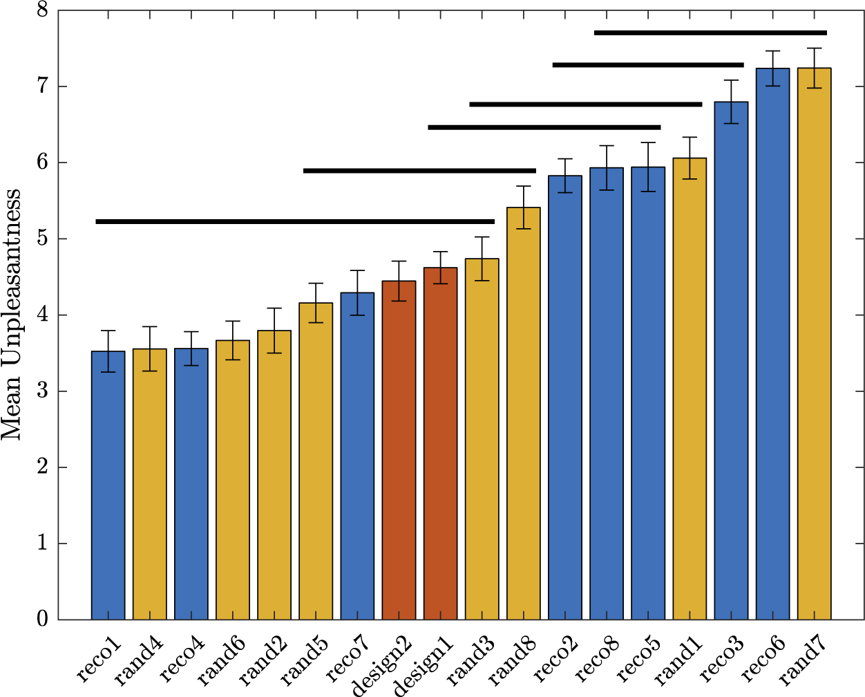
Experiment 3: bar graph of the average value of the detection time for the different quiet vehicle sounds. Nonsignificant differences between pairs of sounds (
 $ p>0.05 $
) are linked with a horizontal line (Tukey’s HSD multiple comparisons test).
$ p>0.05 $
) are linked with a horizontal line (Tukey’s HSD multiple comparisons test).
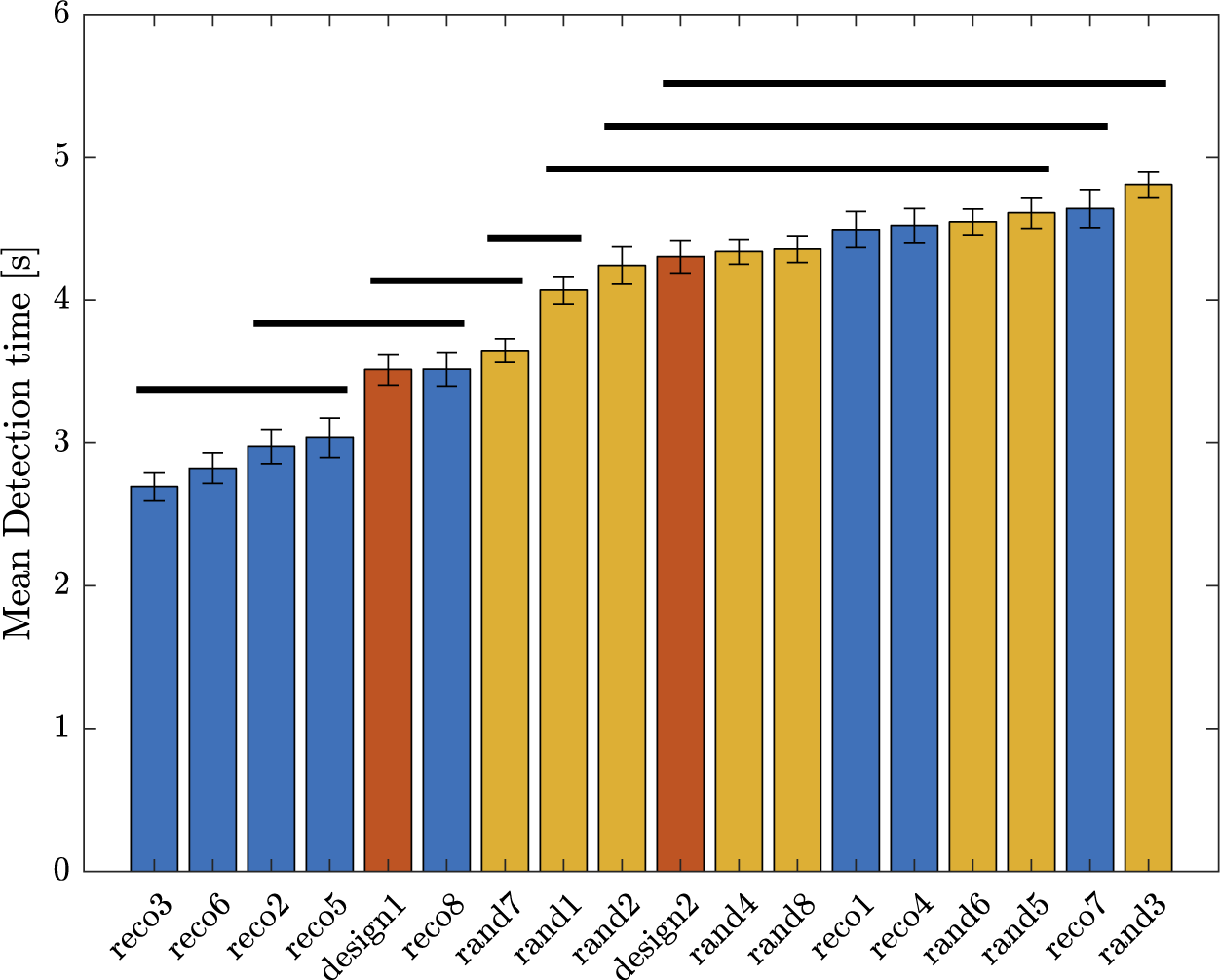
According to unpleasantness (Figure 14), three recommended designs (
 $ reco1,\hskip0.35em reco4,\hskip0.35em reco7 $
) are present in the first group, which also includes the two designed sounds. The designed sounds are rather ‘in the middle’ in terms of unpleasantness. The random and recommended sounds are spread along the unpleasantness range.
$ reco1,\hskip0.35em reco4,\hskip0.35em reco7 $
) are present in the first group, which also includes the two designed sounds. The designed sounds are rather ‘in the middle’ in terms of unpleasantness. The random and recommended sounds are spread along the unpleasantness range.
According to detection time (Figure 15), four recommended designs (
 $ reco3,\hskip0.35em reco6,\hskip0.35em reco2,\hskip0.35em reco5 $
) are present in the first group. Again, the designed sounds are rather ‘in the middle’ regarding detectability. On the other hand, the random sounds are rather on the right side of the scale (large detection time), whereas the recommended sounds are on the left (low detection time). It is clear in Figure 15 that the recommended designs are on average more detectable than the other sounds.
$ reco3,\hskip0.35em reco6,\hskip0.35em reco2,\hskip0.35em reco5 $
) are present in the first group. Again, the designed sounds are rather ‘in the middle’ regarding detectability. On the other hand, the random sounds are rather on the right side of the scale (large detection time), whereas the recommended sounds are on the left (low detection time). It is clear in Figure 15 that the recommended designs are on average more detectable than the other sounds.
Average ratings
To have a more accurate view of the performances of the sounds according to the two objectives, and visualise the trade-off, Figure 16 presents the average performances of each QV sound of the three categories (
 $ Recommended $
,
$ Recommended $
,
 $ Designed $
,
$ Designed $
,
 $ Random $
) according to detection time and unpleasantness. All the sounds can be listened to at the following address, to give a better idea of their design: https://mathieulagrange.github.io/souaille2021interactive/.
$ Random $
) according to detection time and unpleasantness. All the sounds can be listened to at the following address, to give a better idea of their design: https://mathieulagrange.github.io/souaille2021interactive/.
Experiment 3: scatterplot of the average performances of the different quiet vehicle sounds from each category (Recommended, Designed, Random) according to the two objectives, and visualisation of the Pareto front.
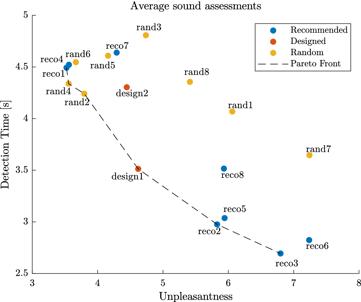
First, we can see that the relative position of the two designed sounds
 $ design1 $
and
$ design1 $
and
 $ design2 $
is similar for Experiment 2 (Figure 13) and Experiment 3 (Figure 16): the sound
$ design2 $
is similar for Experiment 2 (Figure 13) and Experiment 3 (Figure 16): the sound
 $ design1 $
is more unpleasant, but more detectable than
$ design1 $
is more unpleasant, but more detectable than
 $ design2 $
. It belongs to the Pareto front in both cases. Similarly, the relative position of the sounds
$ design2 $
. It belongs to the Pareto front in both cases. Similarly, the relative position of the sounds
 $ rand1 $
to
$ rand1 $
to
 $ rand4 $
is similar for both experiments. This result is a sign of the agreement of the two panels of participants and of the reliability of the experimental protocol.
$ rand4 $
is similar for both experiments. This result is a sign of the agreement of the two panels of participants and of the reliability of the experimental protocol.
Second, the Pareto front is made of three recommended sounds (
 $ reco1 $
,
$ reco1 $
,
 $ reco2 $
,
$ reco2 $
,
 $ reco3 $
), one designed sound (
$ reco3 $
), one designed sound (
 $ Design1 $
) and two random sounds (
$ Design1 $
) and two random sounds (
 $ rand2 $
and
$ rand2 $
and
 $ rand4 $
). The three first recommended sounds (
$ rand4 $
). The three first recommended sounds (
 $ reco1 $
,
$ reco1 $
,
 $ reco2 $
,
$ reco2 $
,
 $ reco3 $
– sounds with the largest probability) belong to the Pareto front. Furthermore, the three other recommended sounds (
$ reco3 $
– sounds with the largest probability) belong to the Pareto front. Furthermore, the three other recommended sounds (
 $ reco4 $
,
$ reco4 $
,
 $ reco5 $
,
$ reco5 $
,
 $ reco6 $
) are very close to the Pareto front. The recommended sounds are rather well represented on the Pareto front.
$ reco6 $
) are very close to the Pareto front. The recommended sounds are rather well represented on the Pareto front.
Third, it is noticeable that the range of the random sounds according to unpleasantness is large, but very narrow for detectability, furthermore located near large detection times: it seems then unlikely to obtain detectable QV sounds by choosing them randomly. Conversely, the ranges of the Recommended sounds according to unpleasantness and detectability are large: the recommended sounds cover a large area of the Pareto front. The recommendations are various, which is an advantage for the definition of different sound prototypes. Furthermore, the most detectable QV sounds are recommended sounds (
 $ reco2 $
,
$ reco2 $
,
 $ reco5 $
,
$ reco5 $
,
 $ reco3 $
,
$ reco3 $
,
 $ reco6 $
). Sounds that are highly detectable seem to be very specific, given that neither random nor designed sounds obtain comparable performances.
$ reco6 $
). Sounds that are highly detectable seem to be very specific, given that neither random nor designed sounds obtain comparable performances.
The two designed sounds obtain average performances, the sounds
 $ design1 $
(Pareto efficient) being an interesting trade-off between the two objectives.
$ design1 $
(Pareto efficient) being an interesting trade-off between the two objectives.
In conclusion, even if all the recommended sounds are not Pareto efficient, they present a large diversity of proposals and are close to the Pareto front (except
 $ reco7 $
and
$ reco7 $
and
 $ reco8 $
).
$ reco8 $
).
This result validates the efficiency of the recommendation method: recommended sounds are on average better than random sounds, and comparable to designed sounds, while offering different trade-offs.
This is illustrated by Figure 17, showing the mean unpleasantness and detection time by sound category.
Experiment 3: scatterplot of the average performances of the different quiet vehicle sound categories (Recommended, Designed, Random) according to the two objectives.
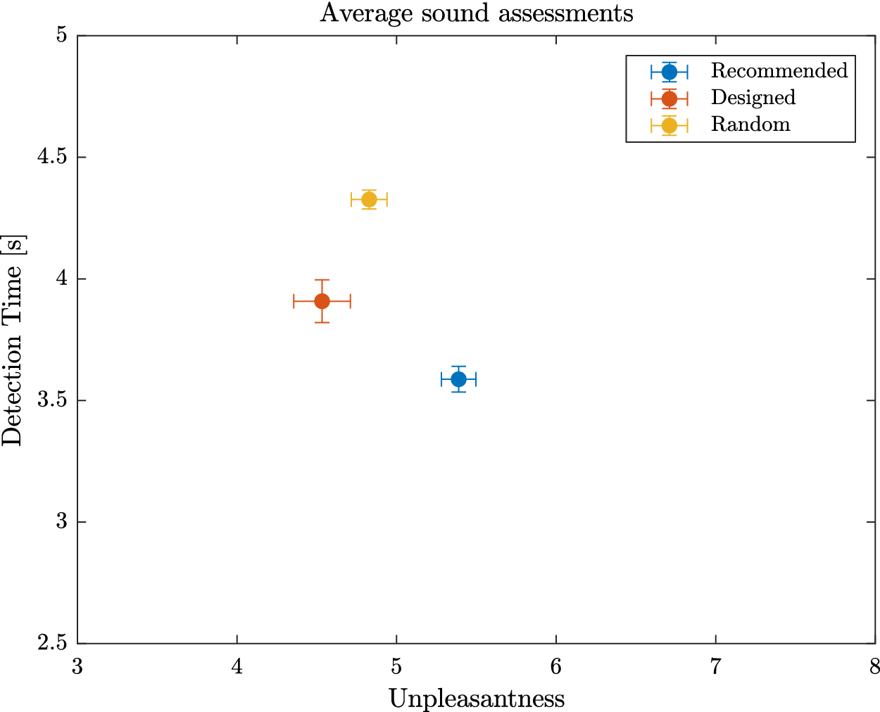
We can then give a rather positive response to question Q2: The recommendation method and the experimental protocol using the IGA allow the determination of very detectable QV sounds, as well as sounds with low unpleasantness.
7. Experiments summary
7.1. Method
The different stages for the definition and the analysis of the three experiments are summarised in Figure 18. The flowchart presents the linking of the different stages, and the analysis of the results to address the research questions Q1 and Q2:
-
(i) Experiment 2 allows the addressing of question Q1, with a comparison at the individual level of the performances of the IGA sounds for detectability and unpleasantness;
-
(ii) Experiment 3 allows the addressing of question Q2, with a comparison of the performances of the recommended sounds for detectability and unpleasantness with an external panel of participants.
Overview of the flowchart for the analysis of Experiments 1–3.
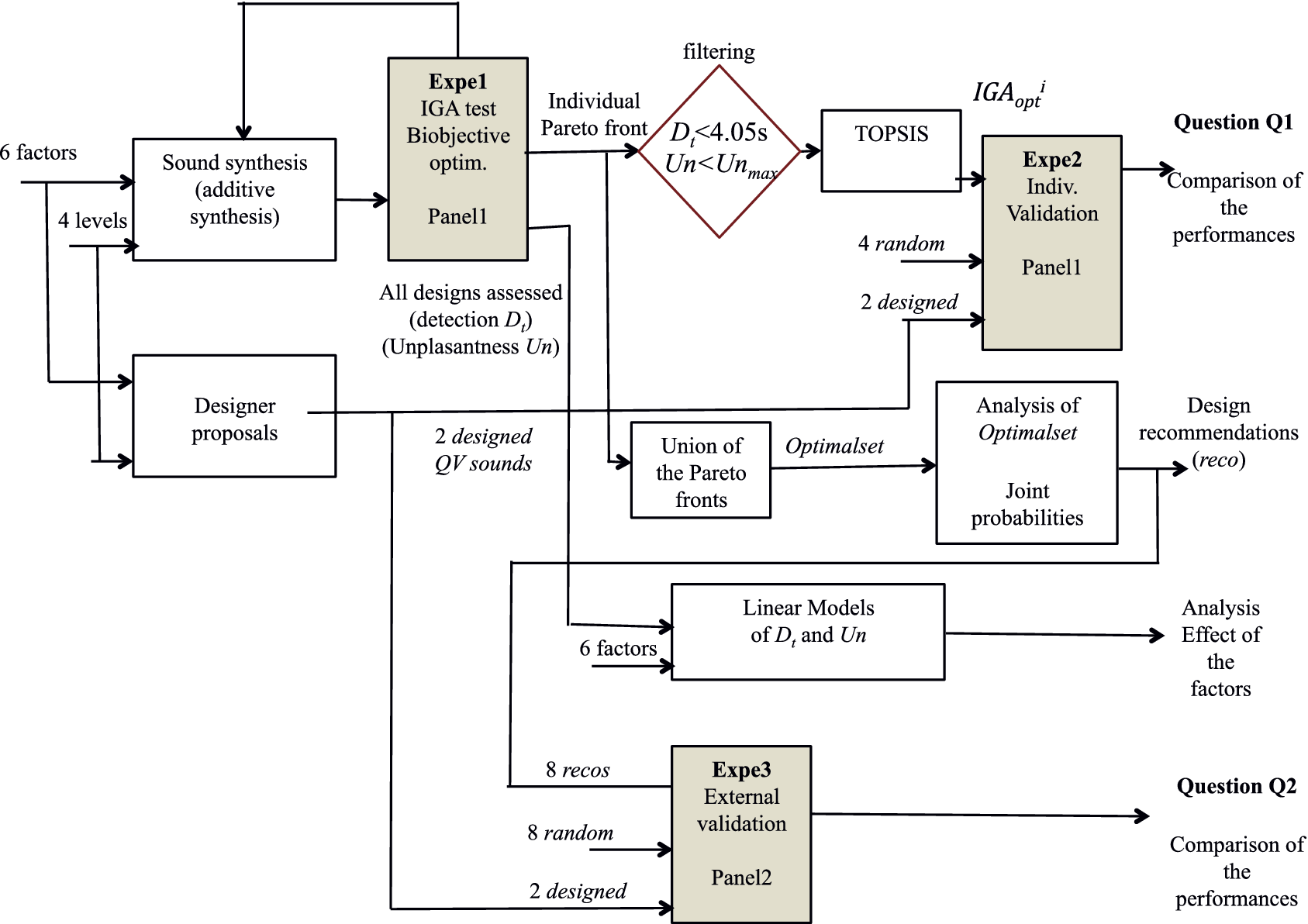

8. Analysis/discussion
This section is dedicated to the implications, in terms of design, of the outcomes of this study.
8.1. Sound level
Even though a study of the acoustical properties of the sounds is out of the scope of this paper, it is important to note that the sounds were not equalised in loudness during the experiments. Since perceived loudness is expected to be an important factor for unpleasantness and detectability, an analysis of the A-weighted equivalent continuous sound level
 $ {L}_{Aeq} $
of the evaluated warning sounds was done for each experiment. More specifically, the correlation between
$ {L}_{Aeq} $
of the evaluated warning sounds was done for each experiment. More specifically, the correlation between
 $ {L}_{Aeq} $
and the two objectives was calculated, based on the raw evaluations of the subjects, after eliminating outliers. The computation of
$ {L}_{Aeq} $
and the two objectives was calculated, based on the raw evaluations of the subjects, after eliminating outliers. The computation of
 $ {L}_{Aeq} $
is provided in the following equation:
$ {L}_{Aeq} $
is provided in the following equation:
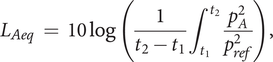 $$ {L}_{Aeq}\hskip0.35em =\hskip0.35em 10\log \left(\frac{1}{t_2-{t}_1}{\int}_{t_1}^{t_2}\frac{p_A^2}{p_{ref}^2}\right), $$
where
 $ {t}_1 $
and
$ {t}_1 $
and
 $ {t}_2 $
are, respectively, the beginning and the end of the signal,
$ {t}_2 $
are, respectively, the beginning and the end of the signal,
 $ {p}_A $
is the instantaneous A-weighted sound pressure and
$ {p}_A $
is the instantaneous A-weighted sound pressure and
 $ {p}_{ref} $
is the reference sound pressure of
$ {p}_{ref} $
is the reference sound pressure of
 $ 20\times {10}^{-6} $
Pascals.
$ 20\times {10}^{-6} $
Pascals.
Table 7 shows the Pearson’s correlation coefficients
 $ \rho $
between the subjects’ evaluations and
$ \rho $
between the subjects’ evaluations and
 $ {L}_{Aeq} $
for all three experiments. It shows a significant positive correlation between unpleasantness and
$ {L}_{Aeq} $
for all three experiments. It shows a significant positive correlation between unpleasantness and
 $ {L}_{Aeq} $
, as well as a significant negative correlation between detection time and
$ {L}_{Aeq} $
, as well as a significant negative correlation between detection time and
 $ {L}_{Aeq} $
. These results confirm a general trend that, on average, the louder a sound is, the faster it is to detect and the more unpleasant it becomes, which is expected.
$ {L}_{Aeq} $
. These results confirm a general trend that, on average, the louder a sound is, the faster it is to detect and the more unpleasant it becomes, which is expected.
Pearson’s correlation coefficients between
 $ {L}_{Aeq} $
and the two objectives, computed from all subjects’ evaluations, without any pre-processing. All coefficients are statistically significant (
$ {L}_{Aeq} $
and the two objectives, computed from all subjects’ evaluations, without any pre-processing. All coefficients are statistically significant (
 $ p<0.001 $
).
$ p<0.001 $
).
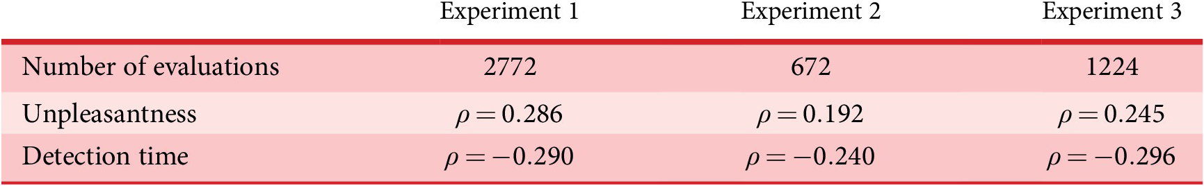
However, the sound level is not a relevant explicating factor. For example, the
 $ {L}_{Aeq} $
is equal to 77 dB for
$ {L}_{Aeq} $
is equal to 77 dB for
 $ rand2 $
and 75 dB for
$ rand2 $
and 75 dB for
 $ reco2 $
, but
$ reco2 $
, but
 $ \mathit{\operatorname{rand}}2 $
is significantly less unpleasant (Figure 13) and significantly less detectable (Figure 14) than
$ \mathit{\operatorname{rand}}2 $
is significantly less unpleasant (Figure 13) and significantly less detectable (Figure 14) than
 $ reco2 $
. To better explain the differences between the sounds, spectral information should be considered. The sound level alone would be insufficient to make design recommendations.
$ reco2 $
. To better explain the differences between the sounds, spectral information should be considered. The sound level alone would be insufficient to make design recommendations.
8.2. QV sound design using an IGA
The first experiment showed that an IGA can be used to interactively explore a sound design space and to define efficient solutions for a bi-objective optimisation problem. This is consistent with previous studies showing the application of IGAs as interactive design tools to address complex perceptual dimensions or affordances (Brintrup et al. Reference Brintrup, Ramsden, Takagi and Tiwari2008; Mata et al. Reference Mata, Fadel, Garland and Zanker2018). In particular, when the two dimensions are conflicting, an IGA may provide efficient designs because interactions between variables are integrated during the interactive solutions search. The linear models without interactions fitted to the data showed opposite effects of the factors on the two objectives, making them ineffective for delivering relevant recommendations.
We believe that an IGA is not intended to replace a designer. Rather, the method could be seen as a complementary tool to assist the work of a sound designer, when the perceptual dimensions are complex or even conflicting. A designer can, for example, perform Experiment 1, in order to get a set of Pareto optimal solutions. These solutions could be considered as ‘presets’ of the sound synthesis method, that could be next ‘fine-tuned’ by the designer, using additional constraints. For QV sounds, constraints related to the brand identity may be, for example, particularly important. This idea is similar to the concept of ‘perceptually relevant presets’ of a musical synthesiser, presented in Roche (Reference Roche2020). The diversity of the proposals on the Pareto front is also a strong point of the method, in order for the designer to propose several prototypes to stakeholders. In a customisation perspective of the QV sound, it could also be interesting to present to customers via a Web interface a way to customise the sound of their vehicle using IGA. In this study, we did not take into account legal or technical considerations regarding the design. An important advantage of the proposed approach is that those constraints can easily be included in the optimisation process, either directly in the sound synthesis method, or as optimisation constraints.
8.3. Design recommendation method
Recommended sound features
The recommendation method presented allows the uncovering of combinations of the levels of the variables that are efficient for the objectives considered in the study. According to our results, there are four combinations of the variables (A, B, C, D) and two combinations of (E, F) that are recommended (see Table 6):
-
(i) A3 B2 C2 D2;
-
(ii) A1 B4 C4 D4;
-
(iii) A2 B4 C4 D4;
-
(iv) A1 B2 C4 D2;
-
(v) A4 B3 C4 D2;
-
(vi) E1 F1 (no modulation);
-
(vii) E3 F2 (modulation 5 Hz – 17%).
Three pairs of sounds (
 $ reco1,\hskip0.35em reco4 $
), (
$ reco1,\hskip0.35em reco4 $
), (
 $ reco3,\hskip0.35em reco6 $
) and (
$ reco3,\hskip0.35em reco6 $
) and (
 $ reco2,\hskip0.35em reco5 $
) are pairwise identical on variables (A, B, C, D), and the only difference is that the second sound of the pair possesses an amplitude modulation (E3 F2). The perception of each pair is similar, the sounds being close on the plane of the two objectives (Figure 16), meaning that the effect of the variables (E, F) on the objectives is weak.
$ reco2,\hskip0.35em reco5 $
) are pairwise identical on variables (A, B, C, D), and the only difference is that the second sound of the pair possesses an amplitude modulation (E3 F2). The perception of each pair is similar, the sounds being close on the plane of the two objectives (Figure 16), meaning that the effect of the variables (E, F) on the objectives is weak.
However, all the recommended designs are combinations of variable levels that affect the objectives in opposite ways: none of the recommended designs have a value of 1 or 4 for all variables and some designs have variable values that go against the linear model’s prediction. For example, considering the resemblance to an ICE vehicle,
 $ reco2 $
has only engine-like sound (A1 and C4), but is very unpleasant, whereas
$ reco2 $
has only engine-like sound (A1 and C4), but is very unpleasant, whereas
 $ reco7 $
has no engine-like component (A4), but is much less unpleasant. This illustrates that there are interactions between the design variables, and that in order to minimise both objectives, design rules have to consider groups of variables simultaneously.
$ reco7 $
has no engine-like component (A4), but is much less unpleasant. This illustrates that there are interactions between the design variables, and that in order to minimise both objectives, design rules have to consider groups of variables simultaneously.
A future work would be to analyse the recommended sounds according to features of the signal, in order to extract design rules. Indeed, the recommended sounds are diverse at the design variable level, and it would be useful to know what characterises them acoustically, apart from the sound level.
Benefits and limitations of the method
The recommended sounds represent a diverse set of solutions to the design problem. Designers may take them into account, and tune them further according to personal preferences and other constraints or objectives that are not taken into account in the objective functions optimised. These sounds are relevant examples with varied but good performances. While the sounds from
 $ Optimalset $
are good solutions from each subject’s point of view, the recommended sounds account for the perception of a whole subject group. This is particularly relevant for real-world problems, where a product’s sound design has to fulfil its purpose for as many people as possible, in the target audience.
$ Optimalset $
are good solutions from each subject’s point of view, the recommended sounds account for the perception of a whole subject group. This is particularly relevant for real-world problems, where a product’s sound design has to fulfil its purpose for as many people as possible, in the target audience.
The fact that the two designed sounds were not recommended shows that even though the recommendation method is able to find some interesting sounds, it is unable to find all of them. It can be due either to the recommendation method, or to the IGA experiment. This is a limit of the method, which could not capture all the relevant trade-offs for the problem.
The efficiency of the recommendation method depends on the number of occurrences of the same designs in the middle area of the Pareto front. If there is a disagreement between the subjects, the recommendation method is unable to capture these multiple designs. This could explain why the recommended sounds tend to be located at the extremes of the Pareto front. The method assumes that there are some acoustic features that contribute to the perception of unpleasantness and detectability, in a similar way across individuals. Studies on this topic (Misdariis et al. Reference Misdariis, Gruson and Susini2013; Lee et al. Reference Lee, Lee, Shin and Han2017) suggest that such features exist. If such features did not exist, the IGA could still be used for customisation, but there would be nothing to capture on the group level for the recommendation method. The results of Experiment 3 suggest that there is more inter-individual variability in the perception of what constitutes a good compromise between the objectives, than there is regarding what makes a sound extreme according to these same objectives.
Another explanation that can be proposed is that the IGA tends to find solutions that are dense at the extremes of the Pareto front, while being sparser in the middle. Further studies are needed to confirm this intuition. Nevertheless, the recommendations remain relevant, as some of them are on par with the second proposal of the designer, the sound
 $ design2 $
.
$ design2 $
.
Future work and applications
A first obvious application of the proposed method would be for the design of other sounds with similar conflicting objectives, such as alarm or mobile phone sounds.
A second important application of the recommendation method would be to investigate perceptual dimensions that are very specific, related to an atypical panel of users (amateur of very sporty cars, blind people etc.). In this case, the designer could use the recommendations based on assessments of this panel to develop prototypes or archetypal sounds. The development of sounds for very sporty cars would be, for example, a relevant application use case of the proposed method.
More generally, the proposed method applies to any problem dealing with the optimisation of a parametrised design, according to one or several perceptual quantities, as long as the evaluation task is simple and short enough to allow for interactive optimisation. Thus, it is not limited to sound design, but can also apply to product shape design (e.g., Mata et al. Reference Mata, Fadel, Garland and Zanker2018). However, if the parameters take continuous values, the design recommendation method should be adapted (by, e.g., estimating probability density functions).
As it was done in this study, an IGA can also be used to study the dependencies between the design variables. When trying to build a model through a DOE approach, this information could be used to make an informed choice of the interaction terms to consider.
9. Conclusion
In this paper, we presented a computational method to perform design recommendations based on an experiment with an IGA. The application is the bi-objective optimisation of the unpleasantness and the detectability of sounds for QV, and uses listening tests with a panel of participants and an IGA for the multiobjective optimisation. The results showed that (i) the individual sounds defined by the IGA perform well regarding the optimisation problem when compared with other QV sounds proposals and (ii) the design recommendations allow the definition of a large diversity of sounds. Those sounds are found to be well performing on average when compared with other proposals. In particular, some of the recommended sounds obtained very good performances in terms of detectability.
The proposed design method is rather generic, as other characteristics than detectability and unpleasantness can be optimised. For example, the sportiness of QV sounds could be investigated, as it presents a challenge for manufacturer because of the lack of background knowledge on this topic. The agreement with the brand image could also be an interesting perceptual dimension.
In light of those results, several research perspectives can be considered. The first one will be to investigate the relationship between signal parameters and the perception of the sounds, in order to extract design rules. The second perspective is the study of more specific perceptual dimensions, related to expert listeners or disabled people. The third perspective will be to guide the parameterisation of the sound synthesis, with considerations for the perceptions of listeners, in order to ensure noticeable differences between sounds available during perceptual IGA experiments.
Acknowledgments
Acknowledgments to the students and professors of the École Centrale de Nantes for their participation to the listening tests.
Financial support
This study was co-financed by the Pays de la Loire region (RFI Ouest Industrie Créative), France, and the European Regional Development Fund.


 Open access