


1 Introduction
High-power laser systems (in the exawatt range and beyond) are highly desirable for addressing several frontier problems in physics, such as electron–positron pair production[
Reference Di Piazza, Müller, Hatsagortsyan and Keitel
1
,
Reference Fedotov, Ilderton, Karbstein, King, Seipt, Taya and Torgrimsson
2
] and the study of quark-gluon plasmas[
Reference McLerran
3
,
Reference Müller
4
]. The advent of high-intensity lasers has created a pressing demand for optical systems capable of withstanding extreme power levels while still enabling precise control and manipulation of light. In this context, plasma emerges as an ideal optical medium, offering exceptional resilience where conventional solid-state optics would fail. Being already ionized, plasma can tolerate much higher intensities compared to the (
 ${\sim} {10}^{13}\ \mathrm{W}/{\mathrm{cm}}^2$
)[
Reference Stuart, Feit, Herman, Rubenchik, Shore and Perry
5
,
Reference Gamaly, Rode, Luther-Davies and Tikhonchuk
6
] damage threshold of typical solid-state materials. A variety of techniques have been developed to enhance laser intensity. Among them, chirped pulse amplification (CPA) stands out as an ingenious method that overcomes the limitations of solid-state-based optics while still utilizing them, enabling the achievement of intensities in the range of
${\sim} {10}^{13}\ \mathrm{W}/{\mathrm{cm}}^2$
)[
Reference Stuart, Feit, Herman, Rubenchik, Shore and Perry
5
,
Reference Gamaly, Rode, Luther-Davies and Tikhonchuk
6
] damage threshold of typical solid-state materials. A variety of techniques have been developed to enhance laser intensity. Among them, chirped pulse amplification (CPA) stands out as an ingenious method that overcomes the limitations of solid-state-based optics while still utilizing them, enabling the achievement of intensities in the range of
 ${\sim} {10}^{18}$
to
${\sim} {10}^{18}$
to
 ${\sim} {10}^{23}\ \mathrm{W}/{\mathrm{cm}}^2$
[
Reference Strickland and Mourou
7
]. Spatiotemporal control of laser pulses has also been achieved with the help of plasma optics[
Reference Riconda and Weber
8
,
Reference Li, Miller, Pierce, Mori, Thomas and Palastro
9
]. The refractive index of the plasma can be tuned by the electron density
${\sim} {10}^{23}\ \mathrm{W}/{\mathrm{cm}}^2$
[
Reference Strickland and Mourou
7
]. Spatiotemporal control of laser pulses has also been achieved with the help of plasma optics[
Reference Riconda and Weber
8
,
Reference Li, Miller, Pierce, Mori, Thomas and Palastro
9
]. The refractive index of the plasma can be tuned by the electron density
 $\left({n}_{\mathrm{e}}\right)$
for the incoming laser frequency
$\left({n}_{\mathrm{e}}\right)$
for the incoming laser frequency
 $\left({\omega}_{\mathrm{l}}\right)$
. Plasma lens configurations have been explored to achieve high intensities through transverse focusing of laser pulses[
Reference Ren, Duda, Hemker, Mori, Katsouleas, Antonsen and Mora
10
]. In addition, laser pulse chirping has also been utilized for temporal compression using plasma mirrors, further contributing to intensity enhancement[
Reference Edwards and Michel
11
].
$\left({\omega}_{\mathrm{l}}\right)$
. Plasma lens configurations have been explored to achieve high intensities through transverse focusing of laser pulses[
Reference Ren, Duda, Hemker, Mori, Katsouleas, Antonsen and Mora
10
]. In addition, laser pulse chirping has also been utilized for temporal compression using plasma mirrors, further contributing to intensity enhancement[
Reference Edwards and Michel
11
].
Curved plasma geometries have recently gained attention for achieving extreme laser intensities. In a curved relativistic mirror (CRM), temporal compression and focusing of Doppler-upshifted light can reach the highest intensities with minimal spot size[ Reference Landecker 12 – Reference Kormin, Borot, Ma, Dallari, Bergues, Aladi, Földes and Veisz 16 ]. While plasma mirrors require petawatt-class lasers and high contrast, a simpler and more robust approach would be to use long, high-energy (joule-level) chirped pulses[ Reference Tümmler, Jung, Stiel, Nickles and Sandner 17 – Reference Nagy, Simon and Veisz 19 ] and to compress them to relativistic intensities over ultrashort ranges, with easier control of contrast and spatiotemporal properties. This has been demonstrated using overdense plasmas with density gradients[ Reference Hur, Ersfeld, Lee, Kim, Roh, Lee, Song, Kumar, Yoffe, Jaroszynski and Suk 20 ]. Other promising methods include Raman amplification of long, high-energy pulses[ Reference Trines, Fiuza, Bingham, Fonseca, Silva, Cairns and Norreys 21 ] and grating-based holographic plasma lenses[ Reference Edwards, Munirov, Singh, Fasano, Kur, Lemos, Mikhailova, Wurtele and Michel 22 , Reference Leblanc, Denoeud, Chopineau, Mennerat, Martin and Quéré 23 ], underscoring the potential of plasma optics to surpass current laser intensity limits.
Building on these advances, a particularly promising frontier involves combining intense laser–plasma interactions with strong magnetic fields for novel optical applications. Magnetized plasmas have already been proposed for a variety of phenomena, including resonant energy absorption[ Reference Dhalia, Juneja and Das 24 – Reference Juneja, Dhalia and Das 27 ], magnetic transparency[ Reference Mandal, Vashistha and Das 28 , Reference Goswami, Maity, Mandal, Vashistha and Das 29 ] and high harmonic generation[ Reference Dhalia, Juneja, Goswami, Maity and Das 30 , Reference Maity, Mandal, Vashistha, Goswami and Das 31 ]. A recent study on magnetized low-frequency (MLF) scattering has been used to amplify laser pulses in strong magnetic fields[ Reference Edwards, Shi, Mikhailova and Fisch 32 ].
Generating magnetic fields of the required strength for these applications, of the order of tens of kilo-teslas (kT), remains a major experimental challenge and is beyond the capabilities of currently available technologies. However, recent breakthroughs have demonstrated fields at the kT level[
Reference Nakamura, Ikeda, Sawabe, Matsuda and Takeyama
33
,
Reference Choudhary, Dhalia, Dam, Parab, Rakeeb, Aparajit, Lad, Ved, Subramanian, Das and Kumar
34
], and emerging proposals suggest that megatesla (MT) fields may soon be achievable. In particular, target geometry-driven mechanisms have even indicated the possibility of generating giga gauss level fields (
 $\sim 0.1\ \mathrm{MT}$
)[
Reference Pan and Murakami
35
,
Reference Korneev, d’Humières and Tikhonchuk
36
]. These advances point toward a promising convergence of plasma-optics techniques and high-field magnetized environments, which could unlock unprecedented opportunities for controlling, compressing and amplifying laser pulses, thereby pushing the frontiers of high-power laser science.
$\sim 0.1\ \mathrm{MT}$
)[
Reference Pan and Murakami
35
,
Reference Korneev, d’Humières and Tikhonchuk
36
]. These advances point toward a promising convergence of plasma-optics techniques and high-field magnetized environments, which could unlock unprecedented opportunities for controlling, compressing and amplifying laser pulses, thereby pushing the frontiers of high-power laser science.
In this article, we propose a novel approach to reach extreme intensities based on chirp pulse compression as well as transverse focusing of a long, negatively chirped, wide spot right circularly polarized (RCP) laser through an underdense magnetized convex-shaped plasma lens. With three-dimensional (3D) and two-dimensional (2D) particle-in-cell (PIC) simulations, we show that reaching extreme intensities is possible using magnetized plasma lenses (MPLs). The schematic of this scheme is shown in Figure 1(a).
Schematic representation (not to scale) of the geometry chosen for 3D simulation. (a) Negatively chirped right circularly polarized laser pulse incident onto a magnetized plasma lens (MPL) immersed in an inhomogeneous magnetic field
 ${\overrightarrow{B}}_{\mathrm{ext}}\left(x,y,z\right)$
. Here
${\overrightarrow{B}}_{\mathrm{ext}}\left(x,y,z\right)$
. Here
 ${w}_{\mathrm{i}},{w}_{\mathrm{f}}$
represent incident and final spot sizes, respectively, and
${w}_{\mathrm{i}},{w}_{\mathrm{f}}$
represent incident and final spot sizes, respectively, and
 ${f}_{\mathrm{init}},{f}_{\mathrm{fin}}$
denote the location of the incident and final focus points of the field, respectively. (b) Simultaneous chirp pulse compression due to inhomogeneous
${f}_{\mathrm{init}},{f}_{\mathrm{fin}}$
denote the location of the incident and final focus points of the field, respectively. (b) Simultaneous chirp pulse compression due to inhomogeneous
 ${\overrightarrow{B}}_{\mathrm{ext}}$
in the MPL. Here
${\overrightarrow{B}}_{\mathrm{ext}}$
in the MPL. Here
 ${\tau}_{\mathrm{i}},{\tau}_{\mathrm{f}}$
represent the pulse duration of the incident chirped pulse and the final compressed pulse, respectively, after passing through the MPL.
${\tau}_{\mathrm{i}},{\tau}_{\mathrm{f}}$
represent the pulse duration of the incident chirped pulse and the final compressed pulse, respectively, after passing through the MPL.

2 Theoretical description
While curved mirror geometries have been extensively studied in plasma optics[
Reference Vincenti
14
,
Reference Quéré and Vincenti
15
], curved lens geometries have attracted less attention. This is mainly because, even in an underdense plasma where the laser frequency
 ${\omega}_{\mathrm{l}}$
exceeds the plasma frequency
${\omega}_{\mathrm{l}}$
exceeds the plasma frequency
 ${\omega}_{\mathrm{pe}}$
, allowing optical transmission, the refractive index of an unmagnetized plasma remains less than unity. Consequently, the phase velocity exceeds the speed of light
${\omega}_{\mathrm{pe}}$
, allowing optical transmission, the refractive index of an unmagnetized plasma remains less than unity. Consequently, the phase velocity exceeds the speed of light
 $\left({v}_\mathrm{p}>c\right)$
, preventing the convergence of incident rays and causing laser pulses to diverge from a convex plasma lens[
Reference Dhalia, Juneja and Das
37
].
$\left({v}_\mathrm{p}>c\right)$
, preventing the convergence of incident rays and causing laser pulses to diverge from a convex plasma lens[
Reference Dhalia, Juneja and Das
37
].
However, the introduction of an external magnetic field adds a crucial tuning parameter: the electron cyclotron frequency
 ${\omega}_{\mathrm{ce}}$
. Along with electron plasma density and laser frequency, this enables precise control over the plasma’s refractive index. Under sufficiently strong magnetic fields, the magnetized response of plasma species can increase the refractive index beyond unity, allowing the plasma to mimic conventional optical materials like glass or solids. This opens the possibility of using MPLs for focusing high-power laser pulses without the typical power threshold limitations posed by solid-state optics.
${\omega}_{\mathrm{ce}}$
. Along with electron plasma density and laser frequency, this enables precise control over the plasma’s refractive index. Under sufficiently strong magnetic fields, the magnetized response of plasma species can increase the refractive index beyond unity, allowing the plasma to mimic conventional optical materials like glass or solids. This opens the possibility of using MPLs for focusing high-power laser pulses without the typical power threshold limitations posed by solid-state optics.
When the magnetic field is aligned along the laser propagation direction, the dispersion relation for the R-mode is given by the following[ Reference Kruer 38 , Reference Chen 39 ]:
 $$\begin{align}{n}_{\mathrm{R}}^2=\frac{c^2}{v_{\mathrm{p}}^2}=1-\frac{\omega_{\mathrm{pe}}^2/{\omega}_{\mathrm{l}}^2}{1-{\omega}_{\mathrm{ce}}/{\omega}_{\mathrm{l}}}.\end{align}$$
For the case
 ${\omega}_{\mathrm{ce}}>{\omega}_{\mathrm{l}}$
, the refractive index
${\omega}_{\mathrm{ce}}>{\omega}_{\mathrm{l}}$
, the refractive index
 $\left({n}_{\mathrm{R}}>1\right)$
results in a phase velocity that is lower than the speed of light within the plasma. Consequently, a magnetized plasma can act as a convex lens, exhibiting focusing properties similar to those of a conventional converging lens. Interestingly, these simple yet profound characteristics of magnetized plasma as a convex lens have recently drawn significant interest[
Reference Dhalia, Juneja and Das
37
].
$\left({n}_{\mathrm{R}}>1\right)$
results in a phase velocity that is lower than the speed of light within the plasma. Consequently, a magnetized plasma can act as a convex lens, exhibiting focusing properties similar to those of a conventional converging lens. Interestingly, these simple yet profound characteristics of magnetized plasma as a convex lens have recently drawn significant interest[
Reference Dhalia, Juneja and Das
37
].
We explore this property to achieve a higher laser field intensity. When the wavelength
 $\left(\lambda \right)$
of the incident light pulse is much smaller than the aperture size
$\left(\lambda \right)$
of the incident light pulse is much smaller than the aperture size
 $\left(\lambda <<D\right)$
, the long laser pulse can be approximated as a ray. Under this approximation the focal length
$\left(\lambda <<D\right)$
, the long laser pulse can be approximated as a ray. Under this approximation the focal length
 $f$
of such a convex MPL can be estimated as follows:
$f$
of such a convex MPL can be estimated as follows:
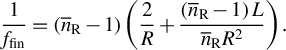 $$\begin{align}\frac{1}{f_{\mathrm{fin}}}=\left({\overline{n}}_{\mathrm{R}}-1\right)\left(\frac{2}{R}+\frac{\left({\overline{n}}_{\mathrm{R}}-1\right)L}{{\overline{n}}_{\mathrm{R}}{R}^2}\right).\end{align}$$
Here,
 $R$
is the radius of curvature of the convex plasma lens and
$R$
is the radius of curvature of the convex plasma lens and
 $L$
is the thickness of the plasma. Here,
$L$
is the thickness of the plasma. Here,
 ${\overline{n}}_{\mathrm{R}}$
is the average refractive index of the plasma lens. This formula is valid as long as the plasma does not absorb any laser energy and behaves like an ideal, thick, solid lens. For the condition
${\overline{n}}_{\mathrm{R}}$
is the average refractive index of the plasma lens. This formula is valid as long as the plasma does not absorb any laser energy and behaves like an ideal, thick, solid lens. For the condition
 ${\omega}_{\mathrm{ce}}>{\omega}_{\mathrm{l}}$
, the laser does not encounter any resonance inside the plasma, resulting in negligible energy absorption for collisionless cases. However, if significant energy is absorbed by the plasma, the focal length predicted by the lens maker’s formula may deviate from the actual value.
${\omega}_{\mathrm{ce}}>{\omega}_{\mathrm{l}}$
, the laser does not encounter any resonance inside the plasma, resulting in negligible energy absorption for collisionless cases. However, if significant energy is absorbed by the plasma, the focal length predicted by the lens maker’s formula may deviate from the actual value.
While the magnetized lens is used for transverse compression of the laser pulse to enhance its intensity, simultaneous temporal compression is achieved by appropriately choosing the chirp of the original laser beam[ Reference Jha, Hemlata and Mishra 40 ]. The group and phase velocities of an RCP wave under R-mode geometry are given by the following[ Reference Dhalia, Juneja, Goswami, Maity and Das 30 ]:
 $$\begin{align}{v}_{\mathrm{p}}\left(\omega, {\omega}_{\mathrm{ce}}\right)=\frac{\omega }{k}=c\sqrt{\frac{\omega \left({\omega}_{\mathrm{ce}}-\omega \right)}{\omega_{\mathrm{pe}}^2+{\omega}_{\mathrm{ce}}\omega -{\omega}^2}},\end{align}$$
 $$\begin{align}{v}_{\mathrm{g}}\left(\omega, {\omega}_{\mathrm{ce}}\right)=\frac{\mathrm{d}\omega }{\mathrm{d}k}=\frac{2{c}^2k\left({\omega}_{\mathrm{ce}}-\omega \right)}{c^2{k}^2+{\omega}_{\mathrm{pe}}^2-3{\omega}^2+2{\omega}_{\mathrm{ce}}\omega }.\end{align}$$
These expressions show that both group and phase velocities decrease as the frequency increases. As a result, launching a negatively chirped long laser pulse, where the high frequency
 $\left({\omega}_{\mathrm{h}}\right)$
leads in time and the low-frequency component
$\left({\omega}_{\mathrm{h}}\right)$
leads in time and the low-frequency component
 $\left({\omega}_{\mathrm{l}}\right)$
trails, through the MPL, enables pulse compression. The difference in group velocities causes the frequency component to converge, leading to a compressed pulse. For a chirped laser pulse, spanning the frequency range
$\left({\omega}_{\mathrm{l}}\right)$
trails, through the MPL, enables pulse compression. The difference in group velocities causes the frequency component to converge, leading to a compressed pulse. For a chirped laser pulse, spanning the frequency range
 $\left({\omega}_{\mathrm{l}},{\omega}_{\mathrm{h}}\right)$
, the required pulse duration
$\left({\omega}_{\mathrm{l}},{\omega}_{\mathrm{h}}\right)$
, the required pulse duration
 $\left(\Delta \tau \right)$
for maximal compression is given by the following:
$\left(\Delta \tau \right)$
for maximal compression is given by the following:
 $$\begin{align}\Delta \tau =\frac{L}{v_{\mathrm{gh}}}-\frac{L}{v_{\mathrm{gl}}}.\end{align}$$
Here,
 ${v}_{\mathrm{gh}}$
and
${v}_{\mathrm{gh}}$
and
 ${v}_{\mathrm{gl}}$
are the group velocities corresponding to
${v}_{\mathrm{gl}}$
are the group velocities corresponding to
 ${\omega}_{\mathrm{h}}$
and
${\omega}_{\mathrm{h}}$
and
 ${\omega}_{\mathrm{l}}$
, respectively, and
${\omega}_{\mathrm{l}}$
, respectively, and
 $L$
is the plasma length along the laser axis. The duration
$L$
is the plasma length along the laser axis. The duration
 $\Delta \tau$
is chosen such that these two frequency components reach the desirable location, typically the plasma edge, for optimal compression, simultaneously. However, defining the chirp profile
$\Delta \tau$
is chosen such that these two frequency components reach the desirable location, typically the plasma edge, for optimal compression, simultaneously. However, defining the chirp profile
 $\omega \left(\tau \right)$
within the interval
$\omega \left(\tau \right)$
within the interval
 $\left(\Delta \tau \right)$
is equally important. For a linear chirp,
$\left(\Delta \tau \right)$
is equally important. For a linear chirp,
 ${\omega \left(\tau \right)={\omega}_0-\alpha \tau}$
, only the extreme frequencies overlap at the plasma edge, while the intermediate frequencies arrive at different times due to the nonlinear dependence of the group velocity on frequency (Equation (4)). This temporal mismatch leads to an extended focal region. To achieve optimal compression, a nonlinear chirp is therefore essential. Such profiles can now be realized through ultrafast pulse shaping techniques[
Reference Weiner
41
–
Reference Wang, Lin, Sheng, Liu, Zhao, Guo, Lu, He, Chen and Yan
45
]. The required chirp profile
${\omega \left(\tau \right)={\omega}_0-\alpha \tau}$
, only the extreme frequencies overlap at the plasma edge, while the intermediate frequencies arrive at different times due to the nonlinear dependence of the group velocity on frequency (Equation (4)). This temporal mismatch leads to an extended focal region. To achieve optimal compression, a nonlinear chirp is therefore essential. Such profiles can now be realized through ultrafast pulse shaping techniques[
Reference Weiner
41
–
Reference Wang, Lin, Sheng, Liu, Zhao, Guo, Lu, He, Chen and Yan
45
]. The required chirp profile
 $\omega \left(\tau \right)$
is obtained by inverting the following:
$\omega \left(\tau \right)$
is obtained by inverting the following:
 $$\begin{align}\tau \left(\omega \right)={\int}_{x_1}^{x_2}\frac{\mathrm{d}x}{v_{\mathrm{g}}\left(\omega, {\omega}_{\mathrm{ce}}\right)},\end{align}$$
where
 ${v}_{\mathrm{g}}\left(\omega, {\omega}_{\mathrm{ce}}\right)$
is the group velocity in the magnetized plasma and
${v}_{\mathrm{g}}\left(\omega, {\omega}_{\mathrm{ce}}\right)$
is the group velocity in the magnetized plasma and
 $L={x}_2-{x}_1$
is the lens length. In our case, the cyclotron frequency varies linearly as
$L={x}_2-{x}_1$
is the lens length. In our case, the cyclotron frequency varies linearly as
 ${\omega}_{\mathrm{ce}}(x)={\omega}_{\mathrm{ce}_0}-p\cdot x$
with
${\omega}_{\mathrm{ce}}(x)={\omega}_{\mathrm{ce}_0}-p\cdot x$
with
 ${\omega}_{\mathrm{ce},0}={eB}_0/{m}_{\mathrm{e}}$
and
${\omega}_{\mathrm{ce},0}={eB}_0/{m}_{\mathrm{e}}$
and
 $p$
characterizing the field gradient.
$p$
characterizing the field gradient.
3 Simulation details
With this straightforward methodology in mind, we performed a proof-of-principle 3D PIC simulation with the massively parallel OSIRIS-4.0 PIC code[
Reference Fonseca, Silva, Tsung, Decyk, Lu, Ren, Mori, Deng, Lee, Katsouleas and Adam
46
,
Reference Davidson, Tableman, An, Tsung, Lu, Vieira, Fonseca, Silva and Mori
47
]. The code uses conventional normalized variables and fields, wherein the length is normalized by the electron skin depth
 $c/{\omega}_{\mathrm{pe}}$
and time by the electron plasma period
$c/{\omega}_{\mathrm{pe}}$
and time by the electron plasma period
 ${\omega}_{\mathrm{pe}}^{-1}$
(see Appendix A for more details).
${\omega}_{\mathrm{pe}}^{-1}$
(see Appendix A for more details).
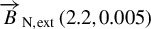
An external magnetic field linearly decreasing along the x-axis, having the following normalized form
 ${B}_{\mathrm{N},\mathit{\operatorname{ext}}}\left({B}_0,\delta \right)$
, has been applied:
${B}_{\mathrm{N},\mathit{\operatorname{ext}}}\left({B}_0,\delta \right)$
, has been applied:
 $$\begin{align}\displaystyle {\overrightarrow{B}}_{\mathrm{N},\operatorname{ext}}\left({B}_0,\delta \right)&=\frac{{\overrightarrow{B}}_{\mathrm{ext}}}{{m}_{\mathrm{e}}c{\omega}_{\mathrm{pe}}/e}=\left[{B}_0-\delta \left(x-110\right)\right]\widehat{i}\nonumber\\ &\quad+\left[0.5\cdot \delta \left(y-110\right)\right]\widehat{j}+\left[0.5\cdot \delta \left(z-110\right)\right]\widehat{k}.\end{align}$$
The choice of the expression in Equation (7) ensures that
 $\nabla \cdot {\overrightarrow{B}}_{\mathrm{ext}}=0$
. We have fixed the value of the parameter
$\nabla \cdot {\overrightarrow{B}}_{\mathrm{ext}}=0$
. We have fixed the value of the parameter
 $\delta =0.005$
and have varied the strength of the magnetic field through
$\delta =0.005$
and have varied the strength of the magnetic field through
 ${B}_0$
in our simulations. For
${B}_0$
in our simulations. For
 ${B}_0=2.2$
, the value of
${B}_0=2.2$
, the value of
 ${\overrightarrow{B}}_{\mathrm{ext}}$
is chosen to range between approximately
${\overrightarrow{B}}_{\mathrm{ext}}$
is chosen to range between approximately
 $15$
and
$15$
and
 $25$
kT for an
$25$
kT for an
 $800\;\mathrm{nm}$
laser and between approximately
$800\;\mathrm{nm}$
laser and between approximately
 $2$
and
$2$
and
 $4$
kT for a
$4$
kT for a
 ${\mathrm{CO}}_2$
laser (
${\mathrm{CO}}_2$
laser (
 $\lambda =9.42\;\mu \mathrm{m}$
). The chosen profile of
$\lambda =9.42\;\mu \mathrm{m}$
). The chosen profile of
 ${\overrightarrow{B}}_{\mathrm{ext}}$
is inspired by the magnetic field lines typically produced by a bar magnet. It is not essential, however, for the field to vary linearly with position. Even an exponentially decaying profile, or a spatially uniform field, would yield a similar magnetic-field-induced focusing effect. The only necessary condition is that
${\overrightarrow{B}}_{\mathrm{ext}}$
is inspired by the magnetic field lines typically produced by a bar magnet. It is not essential, however, for the field to vary linearly with position. Even an exponentially decaying profile, or a spatially uniform field, would yield a similar magnetic-field-induced focusing effect. The only necessary condition is that
 ${\omega}_{\mathrm{ce}}>{\omega}_{\mathrm{l}}>{\omega}_{\mathrm{pe}}$
, ensuring a positive plasma refractive index so that the convex plasma lens focuses the beam at its geometrical focal point.
${\omega}_{\mathrm{ce}}>{\omega}_{\mathrm{l}}>{\omega}_{\mathrm{pe}}$
, ensuring a positive plasma refractive index so that the convex plasma lens focuses the beam at its geometrical focal point.
Magnetic fields of the order of
 $2\ \mathrm{kT}$
have been experimentally achieved for durations of a few hundred picoseconds[
Reference Nakamura, Ikeda, Sawabe, Matsuda and Takeyama
33
,
Reference Choudhary, Dhalia, Dam, Parab, Rakeeb, Aparajit, Lad, Ved, Subramanian, Das and Kumar
34
]. Moreover, laser interaction with an MPL typically occurs over just a few picoseconds during pulse compression and focusing. Therefore, while realizing an optimal MPL for an
$2\ \mathrm{kT}$
have been experimentally achieved for durations of a few hundred picoseconds[
Reference Nakamura, Ikeda, Sawabe, Matsuda and Takeyama
33
,
Reference Choudhary, Dhalia, Dam, Parab, Rakeeb, Aparajit, Lad, Ved, Subramanian, Das and Kumar
34
]. Moreover, laser interaction with an MPL typically occurs over just a few picoseconds during pulse compression and focusing. Therefore, while realizing an optimal MPL for an
 $800\;\mathrm{nm}$
laser may remain technologically challenging at present, the corresponding requirements for a
$800\;\mathrm{nm}$
laser may remain technologically challenging at present, the corresponding requirements for a
 ${\mathrm{CO}}_2$
laser are well within current experimental capabilities.
${\mathrm{CO}}_2$
laser are well within current experimental capabilities.
For definiteness the
 $\left(\lambda =800\;\mathrm{nm}\right)$
laser, having a total energy of
$\left(\lambda =800\;\mathrm{nm}\right)$
laser, having a total energy of
 $0.63\;\mathrm{mJ}$
, pulse duration approximately equal to
$0.63\;\mathrm{mJ}$
, pulse duration approximately equal to
 $80\;\mathrm{fs}$
and spot size approximately equal to
$80\;\mathrm{fs}$
and spot size approximately equal to
 $12\;\mu \mathrm{m}$
, corresponds to an intensity of
$12\;\mu \mathrm{m}$
, corresponds to an intensity of
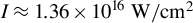 $I\approx 1.36\times {10}^{16}\ \mathrm{W}/{\mathrm{cm}}^2$
and the normalized vector potential amplitude
$I\approx 1.36\times {10}^{16}\ \mathrm{W}/{\mathrm{cm}}^2$
and the normalized vector potential amplitude
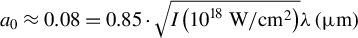 ${a}_0\approx 0.08 = 0.85\cdot \sqrt{I\left({10}^{18}\ \mathrm{W}/{\mathrm{cm}}^2\right)}\lambda \left(\mu \mathrm{m}\right) $
. The laser energy in the simulation has been chosen to be small (
${a}_0\approx 0.08 = 0.85\cdot \sqrt{I\left({10}^{18}\ \mathrm{W}/{\mathrm{cm}}^2\right)}\lambda \left(\mu \mathrm{m}\right) $
. The laser energy in the simulation has been chosen to be small (
 ${\sim}\mathrm{mJ}$
) to comply with the constraint of available computational resources. It is feasible to scale it to several joules by extending the pulse duration to the pico- or nano seconds regime, and enlarging the lens dimensions to the approximately centimeter scale. The focusing element is a convex plasma lens, consisting of fully ionized hydrogen plasmas (see Figure 1), with electron density
${\sim}\mathrm{mJ}$
) to comply with the constraint of available computational resources. It is feasible to scale it to several joules by extending the pulse duration to the pico- or nano seconds regime, and enlarging the lens dimensions to the approximately centimeter scale. The focusing element is a convex plasma lens, consisting of fully ionized hydrogen plasmas (see Figure 1), with electron density
 ${n}_{\mathrm{e}}=0.69{n}_{\mathrm{c}}$
. Here,
${n}_{\mathrm{e}}=0.69{n}_{\mathrm{c}}$
. Here,
 ${n}_{\mathrm{c}}$
is the critical density for the central laser wavelength. For an 800 nm laser pulse, the electron plasma density would be
${n}_{\mathrm{c}}$
is the critical density for the central laser wavelength. For an 800 nm laser pulse, the electron plasma density would be
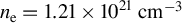 ${n}_{\mathrm{e}}=1.21\times {10}^{21}\;{\mathrm{cm}}^{-3}$
and for a
${n}_{\mathrm{e}}=1.21\times {10}^{21}\;{\mathrm{cm}}^{-3}$
and for a
 ${\mathrm{CO}}_2$
laser, it becomes
${\mathrm{CO}}_2$
laser, it becomes
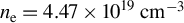 ${n}_{\mathrm{e}}=4.47\times {10}^{19}\ {\mathrm{cm}}^{-3}$
. Such a low-density plasma can be produced experimentally using a foam target based on polymer aerogels[
Reference Rosmej, Gyrdymov, Andreev, Tavana, Popov, Borisenko, Gromov, Gus’kov, Yakhin, Vegunova, Bukharskii, Korneev, Cikhardt, Zähter, Busch, Jacoby, Pimenov, Spielmann and Pukhov
48
,
Reference Khalenkov, Borisenko, Kondrashov, Merkuliev, Limpouch and Pimenov
49
]. The pulse is negatively chirped, with frequency nonlinearly varying within the range
${n}_{\mathrm{e}}=4.47\times {10}^{19}\ {\mathrm{cm}}^{-3}$
. Such a low-density plasma can be produced experimentally using a foam target based on polymer aerogels[
Reference Rosmej, Gyrdymov, Andreev, Tavana, Popov, Borisenko, Gromov, Gus’kov, Yakhin, Vegunova, Bukharskii, Korneev, Cikhardt, Zähter, Busch, Jacoby, Pimenov, Spielmann and Pukhov
48
,
Reference Khalenkov, Borisenko, Kondrashov, Merkuliev, Limpouch and Pimenov
49
]. The pulse is negatively chirped, with frequency nonlinearly varying within the range
 ${\omega}_{\mathrm{l}}\in \left(\mathrm{0.7,1.7}\right){\omega}_{\mathrm{pe}}$
. The nonlinear chirp employed in the simulation is derived from Equation (6) for the external magnetic field
${\omega}_{\mathrm{l}}\in \left(\mathrm{0.7,1.7}\right){\omega}_{\mathrm{pe}}$
. The nonlinear chirp employed in the simulation is derived from Equation (6) for the external magnetic field
 ${\overrightarrow{B}}_{\mathrm{ext}}\left(\mathrm{2.2,0.005}\right)$
and can be represented by a fourth-order polynomial:
${\overrightarrow{B}}_{\mathrm{ext}}\left(\mathrm{2.2,0.005}\right)$
and can be represented by a fourth-order polynomial:
 $$\begin{align}{\omega}_{\mathrm{non}}\left(\tau \right)={\omega}_0+{\omega}_1\tau +{\omega}_2{\tau}^2+{\omega}_3{\tau}^3+{\omega}_4{\tau}^4,\end{align}$$
with coefficients
 ${\omega}_0=1.5276,{\omega}_1=0.0028,{\omega}_2=4.5177\times {10}^{-6},{\omega}_3=5.1483\times {10}^{-7},$
 ${\omega}_4=-1.0223\times {10}^{-8}$
. This profile is employed in simulations with a nonlinear chirp.
${\omega}_4=-1.0223\times {10}^{-8}$
. This profile is employed in simulations with a nonlinear chirp.
4 Results and discussion
We present the observations of 3D simulation for three representative cases corresponding to (i)
 ${B}_0=2.2$
and a linear chirp profile. Cases (ii) and (iii) are for
${B}_0=2.2$
and a linear chirp profile. Cases (ii) and (iii) are for
 ${B}_0=2.2$
and
${B}_0=2.2$
and
 ${B}_0=2.4$
, respectively with a nonlinear chirp profile
${B}_0=2.4$
, respectively with a nonlinear chirp profile
 ${\omega}_{\mathrm{non}}\left(\tau \right)$
defined by Equation (8). It should be noted that this profile has been optimized for
${\omega}_{\mathrm{non}}\left(\tau \right)$
defined by Equation (8). It should be noted that this profile has been optimized for
 ${B}_0=2.2$
. According to the lens maker’s formula (Equation (2)), the predicted focal distances, corresponding to the points of maximum intensity enhancement, are
${B}_0=2.2$
. According to the lens maker’s formula (Equation (2)), the predicted focal distances, corresponding to the points of maximum intensity enhancement, are
 ${f}_{\mathrm{fin}}\sim 216$
for cases (i) and (ii), owing to their identical
${f}_{\mathrm{fin}}\sim 216$
for cases (i) and (ii), owing to their identical
 ${B}_0$
values, and
${B}_0$
values, and
 ${f}_{\mathrm{fin}}\sim 246$
for case (iii). The simulations yield closely matching results, as seen from the intensity peaks in the left-hand column subplots of Figure 2. In these plots, the maximum EMF (electromagnetic field) energy density (blue dashed curve) and the full width at half maximum (FWHM) of the transverse spot (red dashed–dotted curve) are shown as functions of the axial distance
${f}_{\mathrm{fin}}\sim 246$
for case (iii). The simulations yield closely matching results, as seen from the intensity peaks in the left-hand column subplots of Figure 2. In these plots, the maximum EMF (electromagnetic field) energy density (blue dashed curve) and the full width at half maximum (FWHM) of the transverse spot (red dashed–dotted curve) are shown as functions of the axial distance
 $x$
for all three cases. The decrease in FWHM with increasing intensity confirms that transverse focusing is central to the observed enhancement. The vertical black dashed lines mark the axial extent of the plasma lens. The right-hand column plots further illustrate the axial position of the EMF pulse at different times. The results show that maximum amplification indeed occurs at the focal location predicted by Equation (2). Moreover, the temporal pulse duration decreases as the intensity rises, indicating the role of chirp-induced pulse compression. It should be noted that in both case (i) with a linear chirp profile and case (ii) with the optimized chirp profile, a noisy focused pulse is formed. Case (i), in fact, shows a broadened axial region where the focusing occurs. In both these cases, one observes that the focusing being tighter near the lens, the pulse acquires significantly higher amplitude while it is still inside the plasma (see Appendix B). We note that the intensity in fact exceeds
$x$
for all three cases. The decrease in FWHM with increasing intensity confirms that transverse focusing is central to the observed enhancement. The vertical black dashed lines mark the axial extent of the plasma lens. The right-hand column plots further illustrate the axial position of the EMF pulse at different times. The results show that maximum amplification indeed occurs at the focal location predicted by Equation (2). Moreover, the temporal pulse duration decreases as the intensity rises, indicating the role of chirp-induced pulse compression. It should be noted that in both case (i) with a linear chirp profile and case (ii) with the optimized chirp profile, a noisy focused pulse is formed. Case (i), in fact, shows a broadened axial region where the focusing occurs. In both these cases, one observes that the focusing being tighter near the lens, the pulse acquires significantly higher amplitude while it is still inside the plasma (see Appendix B). We note that the intensity in fact exceeds
 ${10}^{18}\ \mathrm{W}/{\mathrm{cm}}^2$
which is known to trigger a nonlinear plasma response[
Reference Li, Miller, Pierce, Mori, Thomas and Palastro
9
], thereby making the pulse significantly noisy. A natural question is whether the outcome can be improved by shifting the focal point slightly outside the plasma lens. To test this, we adjust the magnetic field to
${10}^{18}\ \mathrm{W}/{\mathrm{cm}}^2$
which is known to trigger a nonlinear plasma response[
Reference Li, Miller, Pierce, Mori, Thomas and Palastro
9
], thereby making the pulse significantly noisy. A natural question is whether the outcome can be improved by shifting the focal point slightly outside the plasma lens. To test this, we adjust the magnetic field to
 ${B}_0=2.4$
in case (iii) of our simulations, while keeping all other parameters unchanged. This modification shifts the focal spot further away from the plasma lens. Consequently, there is virtually no amplification within the lens region. In this configuration, the pulse remains clean while exhibiting stronger amplification, making it the most favorable scenario.
${B}_0=2.4$
in case (iii) of our simulations, while keeping all other parameters unchanged. This modification shifts the focal spot further away from the plasma lens. Consequently, there is virtually no amplification within the lens region. In this configuration, the pulse remains clean while exhibiting stronger amplification, making it the most favorable scenario.
The peak of EMF energy density with simultaneous transverse spot-size (FWHM) evolution for a linear chirped laser is shown in (a) for a convex lens immersed in the magnetic field for
 ${\overrightarrow{B}}_{\mathrm{N},\mathit{\operatorname{ext}}}\left(\mathrm{2.2,0.005}\right)$
described in Equation (7). (b) The longitudinal profile of the laser at different times, where peak amplitude is achieved at
${\overrightarrow{B}}_{\mathrm{N},\mathit{\operatorname{ext}}}\left(\mathrm{2.2,0.005}\right)$
described in Equation (7). (b) The longitudinal profile of the laser at different times, where peak amplitude is achieved at
 $t=330{\omega}_{\mathrm{pe}}^{-1}$
; (c), (d) are similarly plotted for the same plasma lens and
$t=330{\omega}_{\mathrm{pe}}^{-1}$
; (c), (d) are similarly plotted for the same plasma lens and
 ${\overrightarrow{B}}_{\mathrm{N},\mathit{\operatorname{ext}}}\left(\mathrm{2.2,0.005}\right)$
but with the nonlinear chirped laser; (e), (f) are plotted for the same plasma lens and a little higher
${\overrightarrow{B}}_{\mathrm{N},\mathit{\operatorname{ext}}}\left(\mathrm{2.2,0.005}\right)$
but with the nonlinear chirped laser; (e), (f) are plotted for the same plasma lens and a little higher
 ${\overrightarrow{B}}_{\mathrm{N},\mathit{\operatorname{ext}}}\left(\mathrm{2.4,0.005}\right)$
but with a linear chirp profile.
${\overrightarrow{B}}_{\mathrm{N},\mathit{\operatorname{ext}}}\left(\mathrm{2.4,0.005}\right)$
but with a linear chirp profile.

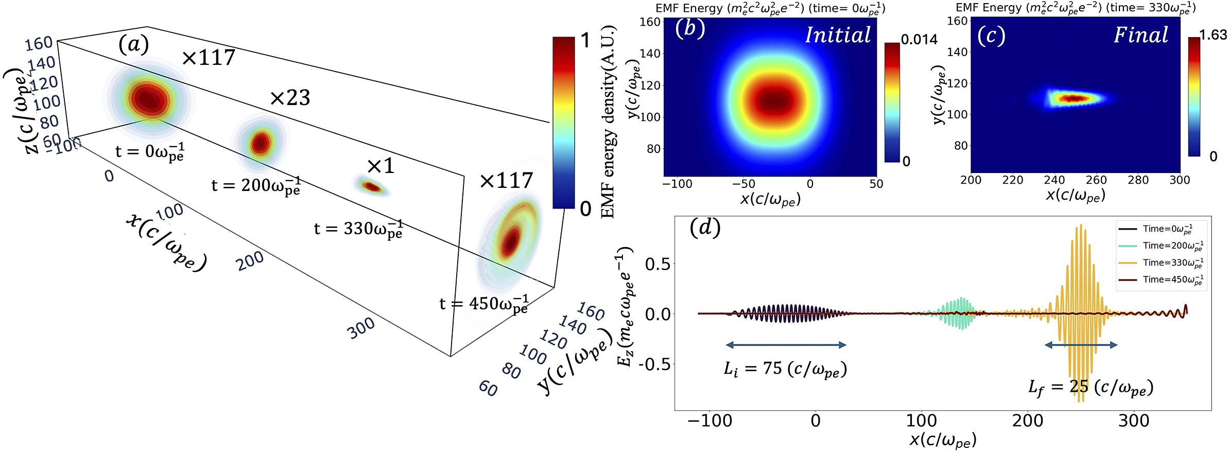
We now examine this best-case scenario, namely case (iii), in greater detail. Figure 3(a) presents the time evolution of the EMF energy density for this case. The chirped Gaussian laser pulse exhibits a significant amplification of EMF energy density (
 $2{a}_0^2$
in normalized units), increasing from an initial peak of
$2{a}_0^2$
in normalized units), increasing from an initial peak of
 $0.014$
(
$0.014$
(
 ${I}_{\mathrm{init}}\approx 1.36\times {10}^{16}\ \mathrm{W}/{\mathrm{cm}}^2$
, Figure 3(b)) to a final peak of
${I}_{\mathrm{init}}\approx 1.36\times {10}^{16}\ \mathrm{W}/{\mathrm{cm}}^2$
, Figure 3(b)) to a final peak of
 $1.63$
(
$1.63$
(
 ${I}_{\mathrm{fin}}\approx 1.58\times {10}^{18}\ \mathrm{W}/{\mathrm{cm}}^2$
, Figure 3(c)) at
${I}_{\mathrm{fin}}\approx 1.58\times {10}^{18}\ \mathrm{W}/{\mathrm{cm}}^2$
, Figure 3(c)) at
 $t=330{\omega}_{\mathrm{pe}}^{-1}$
. This corresponds to nearly a two-order-of-magnitude gain in peak intensity. As the pulse propagates through the MPL, it undergoes both pulse compression and transverse focusing, reaching an optimally compressed and focused state at
$t=330{\omega}_{\mathrm{pe}}^{-1}$
. This corresponds to nearly a two-order-of-magnitude gain in peak intensity. As the pulse propagates through the MPL, it undergoes both pulse compression and transverse focusing, reaching an optimally compressed and focused state at
 ${f}_{\mathrm{fin}}=249c/{\omega}_{\mathrm{pe}}$
. Beyond this focal point, the pulse gradually defocuses and exits the simulation domain. Importantly, no significant reflection losses are observed at the plasma boundaries, indicating efficient transmission through the lens. At
${f}_{\mathrm{fin}}=249c/{\omega}_{\mathrm{pe}}$
. Beyond this focal point, the pulse gradually defocuses and exits the simulation domain. Importantly, no significant reflection losses are observed at the plasma boundaries, indicating efficient transmission through the lens. At
 $t=330{\omega}_{\mathrm{pe}}^{-1}$
, Figure 3(c) shows that the focused pulse remains clean and largely distortion-free. This stability results from the focal spot lying outside the plasma region and the large aperture of the lens (
$t=330{\omega}_{\mathrm{pe}}^{-1}$
, Figure 3(c) shows that the focused pulse remains clean and largely distortion-free. This stability results from the focal spot lying outside the plasma region and the large aperture of the lens (
 ${D=200{l}_N\approx 27\lambda \gg \lambda}$
), which suppresses diffraction from the curved plasma surface. The EMF energy conversion efficiency in the best case – (iii) – is approximately
${D=200{l}_N\approx 27\lambda \gg \lambda}$
), which suppresses diffraction from the curved plasma surface. The EMF energy conversion efficiency in the best case – (iii) – is approximately
 $95.5\%$
. In the other cases – (i) and (ii) – it is approximately
$95.5\%$
. In the other cases – (i) and (ii) – it is approximately
 $67.8\%$
and
$67.8\%$
and
 $62.2\%$
, respectively.
$62.2\%$
, respectively.
(a) The time evolution of an incoming laser pulse launched with a peak amplitude of
 $0.014{m}_{\mathrm{e}}^2{c}^2{\omega}_{\mathrm{pe}}^2{e}^{-2}$
(
$0.014{m}_{\mathrm{e}}^2{c}^2{\omega}_{\mathrm{pe}}^2{e}^{-2}$
(
 $\times 117$
zoom) at
$\times 117$
zoom) at
 $t=0{\omega}_{\mathrm{pe}}^{-1}$
and a maximum compressed and focused pulse achieved at a location
$t=0{\omega}_{\mathrm{pe}}^{-1}$
and a maximum compressed and focused pulse achieved at a location
 ${f}_{\mathrm{fin}}=249c/{\omega}_{\mathrm{pe}}$
at time
${f}_{\mathrm{fin}}=249c/{\omega}_{\mathrm{pe}}$
at time
 $t=330{\omega}_{\mathrm{pe}}^{-1}$
with a peak amplitude reaching
$t=330{\omega}_{\mathrm{pe}}^{-1}$
with a peak amplitude reaching
 $1.63{m}_{\mathrm{e}}^2{c}^2{\omega}_{\mathrm{pe}}^2{e}^{-2}$
(
$1.63{m}_{\mathrm{e}}^2{c}^2{\omega}_{\mathrm{pe}}^2{e}^{-2}$
(
 $\sim 117$
-fold increase); afterwards it again diverges. (b), (c) Surface projection in the
$\sim 117$
-fold increase); afterwards it again diverges. (b), (c) Surface projection in the
 $x-y$
plane at the center
$x-y$
plane at the center
 $z=110c/{\omega}_{\mathrm{pe}}$
of EMF energy density for the initial and final maximum compressed and focused pulse. (d) One-dimensional snapshot of the longitudinal pulse profile at various times. This clearly shows that the chirp pulse is compressed by
$z=110c/{\omega}_{\mathrm{pe}}$
of EMF energy density for the initial and final maximum compressed and focused pulse. (d) One-dimensional snapshot of the longitudinal pulse profile at various times. This clearly shows that the chirp pulse is compressed by
 $1/3$
times from the MPL.
$1/3$
times from the MPL.
To confirm that the increased intensity inside the plasma lens is responsible for the detrimental effect, we performed simulations with higher incident intensities while keeping all other parameters fixed. The results, shown in Figure 4, clearly demonstrate that amplification decreases with increasing incident energy, and in each case, intensity enhancement occurs within the plasma region. This behavior can be understood as follows: with higher incident intensity, the relativistic factor
 ${\gamma}_{\mathrm{max}}$
increases, which in turn reduces the electron cyclotron frequency according to
${\gamma}_{\mathrm{max}}$
increases, which in turn reduces the electron cyclotron frequency according to
 ${\omega}_{\mathrm{ce}}={\omega}_{\mathrm{ce}0}/{\gamma}_{\mathrm{max}}$
. Thus, higher intensity drives
${\omega}_{\mathrm{ce}}={\omega}_{\mathrm{ce}0}/{\gamma}_{\mathrm{max}}$
. Thus, higher intensity drives
 ${\gamma}_{\mathrm{max}}$
to values that satisfy the resonance condition
${\gamma}_{\mathrm{max}}$
to values that satisfy the resonance condition
 ${\omega}_{\mathrm{ce}}\approx {\omega}_{\mathrm{l}}$
inside the plasma. Under such circumstances, irreversible resonant heating dominates, leading to a reduced net intensity gain
${\omega}_{\mathrm{ce}}\approx {\omega}_{\mathrm{l}}$
inside the plasma. Under such circumstances, irreversible resonant heating dominates, leading to a reduced net intensity gain
 $\left({I}_{\mathrm{f}}/{I}_0\right)$
. A possible remedy is to choose a larger value of
$\left({I}_{\mathrm{f}}/{I}_0\right)$
. A possible remedy is to choose a larger value of
 ${B}_0$
, thereby shifting the focal point further outside the plasma lens. In fact, the parameter
${B}_0$
, thereby shifting the focal point further outside the plasma lens. In fact, the parameter
 ${B}_0$
here defining the magnetic field profile turns out to be an important tuning parameter, as shown in Appendix C. To reach the extreme intensities it is necessary to increase the system parameters to larger lengths. We propose a scaling law for the same using 2D simulations (see Appendix D).
${B}_0$
here defining the magnetic field profile turns out to be an important tuning parameter, as shown in Appendix C. To reach the extreme intensities it is necessary to increase the system parameters to larger lengths. We propose a scaling law for the same using 2D simulations (see Appendix D).
(a) The ratio of final and initial intensity as a function of initial intensity. (b) The kinetic energy absorbed by the electrons in plasma with time. The black dashed line represents the laser exiting time from the plasma lens.

Normalized EMF energy density evolution in time for cases (i) and (ii) under interaction with MPL, shown in panels (a) and (b), respectively. At each time t, a
 $\left(\times M\right)$
magnified field has been plotted.
$\left(\times M\right)$
magnified field has been plotted.

5 Conclusion
In conclusion, we propose a curved plasma lens scheme that employs magnetized plasma optics to achieve large intensity gains from low-intensity, high-energy and long-duration pulses. A negatively chirped Gaussian beam undergoes self-compression and self-focusing due to the combined effect of an inhomogeneous magnetic field and a curved plasma geometry, reaching its shortest duration and smallest waist at the plasma lens focus. Unlike curved mirror concepts in unmagnetized plasmas that demand petawatt intensities[ Reference Vincenti 14 , Reference Quéré and Vincenti 15 ], our approach requires only modest initial intensities with large focal spots and longer pulse durations.
The evolution of peak EMF energy amplitude for different cases of applied values of
 ${B}_0$
in
${B}_0$
in
 ${\overrightarrow{B}}_{\mathrm{N},\mathit{\operatorname{ext}}}$
performed with 2D PIC simulations.
${\overrightarrow{B}}_{\mathrm{N},\mathit{\operatorname{ext}}}$
performed with 2D PIC simulations.

Appendix A. Simulation details
The 3D simulations were run on a local machine with 96 cores for approximately
 $120$
hours (
$120$
hours (
 $\approx \mathrm{11,520}$
core-hours), using optimized convex lens geometry and a chirped right-hand circularly polarized (RCP) Gaussian laser in the presence of an external magnetic field. Particle weighting used cubic interpolation on a staggered Yee grid, and the regular Yee solver was used to update the fields. The simulation domain is discretized into
$\approx \mathrm{11,520}$
core-hours), using optimized convex lens geometry and a chirped right-hand circularly polarized (RCP) Gaussian laser in the presence of an external magnetic field. Particle weighting used cubic interpolation on a staggered Yee grid, and the regular Yee solver was used to update the fields. The simulation domain is discretized into
 $1840\times 880\times 880$
cells with spatial resolution of
$1840\times 880\times 880$
cells with spatial resolution of
 $\mathrm{d}x= \mathrm{d}y= \mathrm{d}z=0.25c/{\omega}_{\mathrm{pe}}$
and temporal resolution of
$\mathrm{d}x= \mathrm{d}y= \mathrm{d}z=0.25c/{\omega}_{\mathrm{pe}}$
and temporal resolution of
 $\mathrm{d}t=0.05{\omega}_{\mathrm{pe}}^{-1}$
.
$\mathrm{d}t=0.05{\omega}_{\mathrm{pe}}^{-1}$
.
The plasma lens has a homogeneous density and is finite only within the following region:
 $$\begin{align}&{n}_{\mathrm{e}}={n}_0,\nonumber\\{c}_0{\left(\sqrt{y^2+{z}^2}-110\right)}^2+60&\le x\le -{c}_0{\left(\sqrt{y^2+{z}^2}-110\right)}^2+160.\end{align}$$
Here, parameter
 ${c}_0$
determines the shape of the plasma and has been chosen as
${c}_0$
determines the shape of the plasma and has been chosen as
 $0.005$
. The radius of curvature for such a lens turns out to be
$0.005$
. The radius of curvature for such a lens turns out to be
 $R=100c/{\omega}_{\mathrm{pe}}$
. The incident laser pulse duration is
$R=100c/{\omega}_{\mathrm{pe}}$
. The incident laser pulse duration is
 $\Delta \tau =154{\omega}_{\mathrm{pe}}^{-1}$
and the spot size has a diameter of
$\Delta \tau =154{\omega}_{\mathrm{pe}}^{-1}$
and the spot size has a diameter of
 $80c/{\omega}_{\mathrm{pe}}$
. Thus, the spot size is considerably small compared to the transverse dimension of the plasma lens
$80c/{\omega}_{\mathrm{pe}}$
. Thus, the spot size is considerably small compared to the transverse dimension of the plasma lens
 $D=200c/{\omega}_{\mathrm{pe}}$
. This minimizes the effect of spherical aberration[
Reference Li, Hu, Zhou, Zhang, Wang, Gu, Sattar, Cheng and Guo
50
]. The total run time of the simulation was
$D=200c/{\omega}_{\mathrm{pe}}$
. This minimizes the effect of spherical aberration[
Reference Li, Hu, Zhou, Zhang, Wang, Gu, Sattar, Cheng and Guo
50
]. The total run time of the simulation was
 $460{\omega}_{\mathrm{pe}}^{-1}$
. The dynamics of both electrons and ions have been considered in the simulation.
$460{\omega}_{\mathrm{pe}}^{-1}$
. The dynamics of both electrons and ions have been considered in the simulation.
Appendix B. Evolution of electromagnetic field energy density for cases (i) and (ii)
Figure 5 shows the time evolution of EMF energy density in cases (i) and (ii). Compression and focusing take place in both these cases. However, a comparison with Figure 3 for case (iii) in the main text shows that the quality of compression in these cases is not good. While case (i), shown in Figure 5, shows elongated focus in the longitudinal direction, for case (ii) the energy gets reflected from the edge of the lens and propagates inwards, thereby causing a loss of energy.
Appendix C. Amplification by tuning the parameter
 ${B}_0$

Two-dimensional simulations for various values of the parameter
 ${B}_0$
have been carried out spanning the range
${B}_0$
have been carried out spanning the range
 ${B}_0\in \left[\mathrm{2.2,2.6}\right]$
. It can be observed from Figure 6 that the best result is obtained for
${B}_0\in \left[\mathrm{2.2,2.6}\right]$
. It can be observed from Figure 6 that the best result is obtained for
 ${B}_0=2.4$
. Thus, the profile of the magnetic field acts as an important tuning parameter.
${B}_0=2.4$
. Thus, the profile of the magnetic field acts as an important tuning parameter.
Appendix D. Two-dimensional simulations with increased system parameters and scaling behavior
We conducted 2D PIC simulations by successively doubling and quadrupling the characteristic system parameters, thereby scaling both the laser and plasma parameters accordingly. The applied external magnetic fields were chosen to be slightly higher, with
 ${\overrightarrow{B}}_{\mathrm{double}}={\overrightarrow{B}}_{\operatorname{ext},2\mathrm{D}}\left({B}_0=2.5,\delta =0.0025\right)$
and
${\overrightarrow{B}}_{\mathrm{double}}={\overrightarrow{B}}_{\operatorname{ext},2\mathrm{D}}\left({B}_0=2.5,\delta =0.0025\right)$
and
 ${\overrightarrow{B}}_{\mathrm{quad}}={\overrightarrow{B}}_{\operatorname{ext},2\mathrm{D}}\left({B}_0=2.5,\delta =0.00125\right)$
, in order to avoid resonance matching within the plasma.
${\overrightarrow{B}}_{\mathrm{quad}}={\overrightarrow{B}}_{\operatorname{ext},2\mathrm{D}}\left({B}_0=2.5,\delta =0.00125\right)$
, in order to avoid resonance matching within the plasma.
The laser pulse width and focal spot size were taken as
 ${w}_{\mathrm{double}}=160c/{\omega}_{\mathrm{pe}}$
,
${w}_{\mathrm{double}}=160c/{\omega}_{\mathrm{pe}}$
,
 $\Delta {\tau}_{\mathrm{double}}=308{\omega}_{\mathrm{pe}}^{-1}$
and
$\Delta {\tau}_{\mathrm{double}}=308{\omega}_{\mathrm{pe}}^{-1}$
and
 ${w}_{\mathrm{quad}}=320c/{\omega}_{\mathrm{pe}}$
,
${w}_{\mathrm{quad}}=320c/{\omega}_{\mathrm{pe}}$
,
 $\Delta {\tau}_{\mathrm{quad}}=612{\omega}_{\mathrm{pe}}^{-1}$
, respectively. The corresponding frequency chirp profiles for these cases were obtained from Equation (6), and implemented using fitted fourth-order polynomials, denoted as
$\Delta {\tau}_{\mathrm{quad}}=612{\omega}_{\mathrm{pe}}^{-1}$
, respectively. The corresponding frequency chirp profiles for these cases were obtained from Equation (6), and implemented using fitted fourth-order polynomials, denoted as
 ${\omega}_{\mathrm{non},\mathrm{double}}$
and
${\omega}_{\mathrm{non},\mathrm{double}}$
and
 ${\omega}_{\mathrm{non},\mathrm{quad}}$
in the simulations.
${\omega}_{\mathrm{non},\mathrm{quad}}$
in the simulations.
Gain in the intensity obtained using 2D PIC simulations with system parameters being enhanced by a multiplicative factor of n.

Similarly, the physical dimensions of the plasma lens, both its longitudinal length and transverse width, were scaled by factors of two and four, respectively. The corresponding radii of curvature were taken as
 ${R}_{\mathrm{double}}=200{l}_{\mathrm{N}}$
and
${R}_{\mathrm{double}}=200{l}_{\mathrm{N}}$
and
 ${R}_{\mathrm{quad}}=400{l}_{\mathrm{N}}$
.
${R}_{\mathrm{quad}}=400{l}_{\mathrm{N}}$
.
Figure 7 clearly demonstrates that increasing the system parameters leads to a corresponding enhancement in intensity gain, which has been fitted by the scaling relation
 ${\left({I}_{\mathrm{f}}/{I}_0\right)}_{2\mathrm{D}}=25\times {(1.25)}^{n-1}$
for
${\left({I}_{\mathrm{f}}/{I}_0\right)}_{2\mathrm{D}}=25\times {(1.25)}^{n-1}$
for
 $n\ge 1$
. In a 3D geometry, the addition of an extra spatial dimension is expected to further enhance this trend through an additional multiplicative factor. Following this scaling behavior, one can, in principle, extend the plasma and laser spot dimensions approximately to the centimeter scale and the pulse duration approximately to the hundreds of picoseconds range, thereby achieving significantly higher final intensities starting from relatively modest initial laser powers.
$n\ge 1$
. In a 3D geometry, the addition of an extra spatial dimension is expected to further enhance this trend through an additional multiplicative factor. Following this scaling behavior, one can, in principle, extend the plasma and laser spot dimensions approximately to the centimeter scale and the pulse duration approximately to the hundreds of picoseconds range, thereby achieving significantly higher final intensities starting from relatively modest initial laser powers.
Acknowledgements
The authors would like to acknowledge the OSIRIS Consortium, consisting of UCLA and IST (Lisbon, Portugal), for providing access to the OSIRIS 4.0 framework, which is supported by the NSF under ACI-1339893. A.D. acknowledges support from the Anusandhan National Research Foundation (ANRF) of the Government of India through core grant CRG/2022/002782 as well as her J. C. Bose Fellowship grant JCB/2017/000055. The authors would also like to thank the IIT Delhi HPC facility for computational resources. T.D. also wishes to thank the Council for Scientific and Industrial Research (Grant No. 09/086/(1489)/2021-EMR-I) for funding this research.


 Open access