





1 Introduction
In the theory of dynamical systems, it is common to encounter examples of systems with simple governing laws that exhibit highly complex and unpredictable behaviour. Prominent examples include one-dimensional quadratic maps, two-dimensional Hénon quadratic diffeomorphisms and the Lorenz system of quadratic differential equations in three-dimensional Euclidean space. Despite their straightforward formulation, these systems display intricate dynamical properties that have inspired significant mathematical developments over the past few decades.
One of the central areas of investigation in the theory of dynamical systems has been the study of invariant measures that describe the statistical behaviour of these systems over time. Among these, Sinai–Ruelle–Bowen (SRB) measures, also known as physical measures, play a pivotal role. SRB measures are particularly important because they provide a way to understand the asymptotic distribution of orbits for a wide range of initial conditions, typically those that are of full measure with respect to the Lebesgue (volume) measure on the phase space. In other words, they allow us to describe the long-term statistical behaviour of almost all initial points in a given region, making them essential tools for analysing chaotic systems where individual trajectories may be unpredictable, but the statistical distribution of orbits remains stable.
A key area of research in this field involves understanding the conditions under which SRB measures exist, as well as their robustness to perturbations in the system. The continuous dependence of these measures on the underlying dynamics is particularly significant, as it reflects the stability of the system’s statistical properties in response to small changes. This is not only important from a theoretical standpoint, but also has practical implications, as small perturbations often arise in real-world systems due to noise or external influences. In particular, the continuity of the metric entropy—a quantity that measures the complexity and unpredictability of the system—associated with SRB measures is a subject of extensive study. Metric entropy quantifies the rate of information production in the system and is directly related to the degree of chaos present.
Many results in the literature have been devoted to the study of SRB measures and their associated metric entropies in various dynamical settings [Reference Alves1, Reference Alves, Bonatti and Viana2, Reference Alves, Dias, Luzzatto and Pinheiro5, Reference Araujo, Pacifico, Pujals and Viana12, Reference Benedicks and Carleson17–Reference Bowen and Ruelle22, Reference Góra and Boyarsky26, Reference Jakobson28, Reference Lasota and Yorke31–Reference Pesin34, Reference Ruelle38, Reference Sinai40]. These results range from classical systems like hyperbolic maps and diffeomorphisms to more complex systems involving non-uniformly hyperbolic dynamics or systems with piecewise smooth structures. Understanding how SRB measures and their entropies behave under perturbations provides valuable insights into the stability and predictability of chaotic systems, a topic that has been extensively explored previously [Reference Alves, Pumariño and Vigil8, Reference Alves and Soufi10, Reference Alves, Carvalho and Freitas3, Reference Alves, Carvalho and Freitas4, Reference Alves, Oliveira and Tahzibi7–Reference Alves and Viana11, Reference Bahsoun and Ruziboev14, Reference Freitas23, Reference Galatolo and Lucena24, Reference Keller29]. This ongoing research continues to shed light on the delicate interplay between deterministic chaos and statistical regularity, offering a deeper comprehension of the fundamental nature of chaotic dynamical systems.
In this work, we focus on absolutely continuous invariant probability measures (ACIPs), a class of measures that are absolutely continuous with respect to the Lebesgue measure and often coincide with SRB measures in the context of non-uniformly hyperbolic systems. Specifically, we present estimates on the modulus of continuity of the densities and metric entropies of ergodic ACIPs for certain classes of piecewise expanding maps in any finite dimension. These results extend the conclusions of previous works [Reference Alves, Pumariño and Vigil8, Reference Alves and Pumariño9] and provide a deeper understanding of how the statistical properties of such systems behave under perturbations. To achieve this, we employ a result of Galatolo and Lucena in [Reference Galatolo and Lucena24], which enables us to establish the modulus of continuity mentioned above.
Our primary application of these theoretical results is focused on a particular family of two-dimensional tent maps introduced in [Reference Pumariño, Rodríguez, Tatjer and Vigil35]. This family is especially interesting because it is related to limit return maps that arise when a homoclinic tangency is unfolded by a family of three-dimensional diffeomorphisms, as discussed in [Reference Pumariño, Rodríguez, Tatjer and Vigil35, Reference Tatjer41]. In previous works, the existence of ergodic ACIPs for these tent maps was established [Reference Pumariño, Rodríguez, Tatjer and Vigil36] and the continuity of the densities of these measures, along with their entropies was demonstrated [Reference Alves, Pumariño and Vigil8, Reference Alves and Pumariño9]. Building on these foundational results, we now strengthen the previous conclusions by showing that the densities and metric entropies associated with these ACIPs perturbed by size $\delta $
have a modulus of continuity of order
$\delta $
have a modulus of continuity of order $\delta \log \delta $
. Our results are quite sharp for somewhat uniform families of piecewise expanding maps; see [Reference Baladi15, Reference Baladi and Smania16]. We remark that just Hölder continuity could also be deduced from the results of Keller and Liverani in [Reference Keller and Liverani30].
$\delta \log \delta $
. Our results are quite sharp for somewhat uniform families of piecewise expanding maps; see [Reference Baladi15, Reference Baladi and Smania16]. We remark that just Hölder continuity could also be deduced from the results of Keller and Liverani in [Reference Keller and Liverani30].
The continuity of physical measures and their metric entropies plays a fundamental role in understanding the stability of dynamical systems, particularly those exhibiting complex or chaotic behaviour. By addressing the modulus of continuity of both physical measures and their metric entropies, our work aims to provide deeper insights into the intricate relationship between the dynamics of a system and the statistical properties of its invariant measures. Understanding this relationship is key to predicting the robustness of complex dynamical systems under perturbations, a question that has far-reaching implications in various fields, from mathematical theory to applied sciences. This research sheds light on the subtle and quantitative ways in which physical measures and their metric entropy responds to changes in the underlying system, offering a more nuanced understanding of the stability and variability of chaotic systems. Through this investigation, we contribute to the broader goal of characterizing the resilience of dynamical systems to fluctuations, and thus advancing the overall theory of dynamical stability.
1.1 Modulus of continuity
Here, we present the general setting under which our main results will be obtained. Let $\Omega $
be a compact subset of
$\Omega $
be a compact subset of $\mathbb {R}^d$
, for some
$\mathbb {R}^d$
, for some $d\ge 1$
. Consider m the Lebesgue measure on
$d\ge 1$
. Consider m the Lebesgue measure on $\Omega $
and, for each
$\Omega $
and, for each $1\le p\le \infty $
, the respective space
$1\le p\le \infty $
, the respective space $L^p(\Omega )$
endowed with its usual norm
$L^p(\Omega )$
endowed with its usual norm $\|\quad \|_p$
. Absolute continuity will be always meant with respect to m. Let
$\|\quad \|_p$
. Absolute continuity will be always meant with respect to m. Let $(\phi _t)_{t\in I}$
be a family of transformations
$(\phi _t)_{t\in I}$
be a family of transformations $\phi _t: \Omega \to \Omega $
, where I is a metric space. We assume that there exists
$\phi _t: \Omega \to \Omega $
, where I is a metric space. We assume that there exists $N\in \mathbb N\cup \{\infty \}$
and, for each
$N\in \mathbb N\cup \{\infty \}$
and, for each $t\in I$
, there exists an m mod 0 partition
$t\in I$
, there exists an m mod 0 partition $\{ R_{t,i}\}_{i=0}^{N-1}$
of
$\{ R_{t,i}\}_{i=0}^{N-1}$
of $\Omega $
such that each
$\Omega $
such that each $R_{t,i} $
is a closed domain with piecewise
$R_{t,i} $
is a closed domain with piecewise $C^2$
boundary of finite
$C^2$
boundary of finite $(d-1)$
-dimensional measure. We also assume that
$(d-1)$
-dimensional measure. We also assume that
 $$ \begin{align} \phi_{t,i}=\phi_t|_{R_{t,i}} \end{align} $$
is a $C^2$
bijection from
$C^2$
bijection from $\operatorname {int}(R_{t,i})$
, the interior of
$\operatorname {int}(R_{t,i})$
, the interior of $R_{t,i}$
, onto its image, with a
$R_{t,i}$
, onto its image, with a $C^2$
extension to the boundary of
$C^2$
extension to the boundary of $R_{t,i}$
. Consider the Jacobian function
$R_{t,i}$
. Consider the Jacobian function
 $$ \begin{align*}J_{t}=|\!\kern-1pt\det (D\phi_t)|,\end{align*} $$
defined on the (full Lebesgue measure) subset of points in $\Omega $
where
$\Omega $
where $\phi _t$
is differentiable. Next, we state some conditions for our family of maps.
$\phi _t$
is differentiable. Next, we state some conditions for our family of maps.
-
(P1) There exists $\sigma _t>0$
such that for all
$0\le i< N$
and all
$x\in \operatorname {int}(\phi _t(R_{t,i}))$
,
$$ \begin{align*}\| D\phi_{t,i}^{-1}(x)\| \le \sigma_t.\end{align*} $$
$\sigma _t>0$
such that for all
$0\le i< N$
and all
$x\in \operatorname {int}(\phi _t(R_{t,i}))$
,
$$ \begin{align*}\| D\phi_{t,i}^{-1}(x)\| \le \sigma_t.\end{align*} $$




-
(P2) There exists
$\Delta _t\ge 0$
such that for all
$0\le i< N$
and all
$x,y\in \operatorname {int}(R_{t,i})$
,
$$ \begin{align*} \log \frac{J_{ t}(x)}{J_{ t}(y)}\le \Delta_t\,\|\phi_t(x)-\phi_t(y)\|. \end{align*} $$




-
(P3) There exist
$\alpha _t,\beta _t>0$
and, for each
$0\le i< N$
, there exists a
$C^1$
unitary vector field
$X_{t,i}$
on
$\partial \phi _t(R_{t,i})$
(at the points
$x\in \partial \phi _t(R_{t,i})$
where
$\partial \phi _t(R_{t,i})$
is not smooth the vector,
$X_{t,i}(x)$
is a common
$C^1$
extension of
$X_{t,i}$
restricted to each
$(d-1)$
-dimensional smooth component of
$\partial \phi _t(R_{t,i})$
having x in its boundary. The tangent space at any such point is the union of the tangent spaces to the
$(d-1)$
-dimensional smooth components to which that point belongs) such that:-
(a) the line segments joining each
$x\in \partial \phi _t(R_{t,i})$
to
$x+\alpha _t X_{t,i}(x)$
are pairwise disjoint, contained in
$\phi _t(R_{t,i})$
, and their union is a neighbourhood of
$\partial \phi _t(R_{t,i})$
in
$\phi _t(R_{t,i})$
; -
(b) for each
$x{\kern-1pt}\in{\kern-1pt} \partial \phi _t(R_{t,i})$
and
$v{\kern-1pt}\in{\kern-1pt} T_x\partial \phi _t(R_{t,i}){\kern-1pt}\setminus{\kern-1pt} \{0\}$
, we have
${|\kern -1.2pt \sin{\kern-1pt} \angle (v,{\kern-1pt}X_{t,i} (x))|{\kern-1pt}\geq{\kern-1pt} \beta _t}$
, where
$\angle (v,X_{t,i}(x))$
denotes the angle between v and
$X_{t,i}(x)$
.
-














Under these conditions, it was established in [Reference Alves1] (see also [Reference Góra and Boyarsky26] for the case of a finite number of smoothness domains) that each $\phi _t$
has some ergodic absolutely continuous invariant probability measure. Assuming the uniqueness of this measure for each t, the continuity of the measure in relation to the parameter t was also proven in [Reference Alves, Pumariño and Vigil8], under the following uniformity condition:
$\phi _t$
has some ergodic absolutely continuous invariant probability measure. Assuming the uniqueness of this measure for each t, the continuity of the measure in relation to the parameter t was also proven in [Reference Alves, Pumariño and Vigil8], under the following uniformity condition:
-
(U) there exists
$\ell \ge 1$
such that
$\phi _t^j$
satisfies conditions (P1)–(P3) for each
$1\le j\le \ell $
; moreover, there exist
$0<\theta <1$
and
$M>0$
such that, for all
$t\in I$
and
$1\le j\le \ell $
, where
$$ \begin{align*} \sigma_{t,\ell}\bigg(1+\frac1{\beta_{t,\ell}}\bigg)\le \theta,\quad \sigma_{t,j}\bigg(1+\frac1{\beta_{t,j}}\bigg)\le M \quad\text{and}\quad \Delta_{t,j}+ \frac{1}{\alpha_{t,j}\beta_{t,j}} + \frac{\Delta_{t,j }}{\beta_{t,j}} \le M, \end{align*} $$
$\sigma _{t,j}, \Delta _{t,j}, \alpha _{t,j},\beta _{t,j}$
are the constants in conditions (P1)–(P3) for the map
$\phi ^j_t$
.




To establish the modulus of continuity of these measures and their entropies, some additional conditions are required. Set for each $s,t\in I$
and
$s,t\in I$
and $0\le i< N$
,
$0\le i< N$
,
 $$ \begin{align*} K_{t,s,i}=\phi_{s,i}^{-1}(\phi_t(R_{t,i})\cap\phi_s(R_{s,i}))\quad\text{and}\quad \psi_{t,s,i}=\phi_{t,i}^{-1}\circ \phi_{s,i}|_{K_{t,s,i}}.\end{align*} $$
Naturally, we consider $\psi _{t,s,i}$
only when
$\psi _{t,s,i}$
only when $K_{t,s,i} \neq \emptyset $
. In fact, conditions (1)–(3) of Theorem A below essentially mean that the sets
$K_{t,s,i} \neq \emptyset $
. In fact, conditions (1)–(3) of Theorem A below essentially mean that the sets $\phi _t(R_{t,i})$
and
$\phi _t(R_{t,i})$
and $\phi _s(R_{s,i})$
are close to each other, and the maps
$\phi _s(R_{s,i})$
are close to each other, and the maps $\phi _{t,i}$
and
$\phi _{t,i}$
and $\phi _{s,i}$
are also close to each other. Let
$\phi _{s,i}$
are also close to each other. Let $\operatorname {id}$
represent the identity map on
$\operatorname {id}$
represent the identity map on $\mathbb {R}^d$
, possibly restricted to some subset of
$\mathbb {R}^d$
, possibly restricted to some subset of $\mathbb {R}^d$
. Define the difference set
$\mathbb {R}^d$
. Define the difference set
 $$ \begin{align*}A=\{s-t: s,t\in I\}. \end{align*} $$
Given a compact set $K\subset \mathbb R^d$
and a function
$K\subset \mathbb R^d$
and a function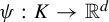 $\psi :K\to \mathbb R^d$
, let
$\psi :K\to \mathbb R^d$
, let
 $$ \begin{align*}\|\psi\|_0=\sup_{x\in K}\|\psi(x)\|,\end{align*} $$
where $\|\cdot \|$
denotes the Euclidean norm in
$\|\cdot \|$
denotes the Euclidean norm in $\mathbb R^d$
. In what follows, we assume
$\mathbb R^d$
. In what follows, we assume $0\log 0=0$
.
$0\log 0=0$
.
Theorem A. Let $(\phi _t)_{t\in I}$
be a family of maps for which condition (U) holds and each
$(\phi _t)_{t\in I}$
be a family of maps for which condition (U) holds and each $\phi _t $
has a unique ergodic absolutely continuous invariant probability measure
$\phi _t $
has a unique ergodic absolutely continuous invariant probability measure $\mu _t$
. Assume that there exists a function
$\mu _t$
. Assume that there exists a function $\mathcal E:A\to \mathbb [0,1)$
such that, for all
$\mathcal E:A\to \mathbb [0,1)$
such that, for all $s,t\in I$
:
$s,t\in I$
:
-
(1)
$ \sum _{i=1}^Nm(\phi _{t,i}^{-1}(\phi _t(R_{t,i})\setminus \phi _s(R_{s,i})))^{1/d}\le \mathcal E(t-s);$
-
(2)
$\sum _{i=1}^N \|\psi _{t,s,i}-\operatorname {id}\!\|_0 \le \mathcal E(t-s)$
; -
(3)
$ \sum _{i=1}^N|{J_s}/{J_t\circ \psi _{t,s,i}}-1|\le \mathcal E(t-s)$
.



Then, there exist $C>0$
and
$C>0$
and $0<\eta <1$
such that, for all
$0<\eta <1$
such that, for all $s,t\in I$
,
$s,t\in I$
,
 $$ \begin{align*}\bigg\|\frac{d{\mu_t}}{dm}-\frac{d{\mu_{s}}}{dm}\bigg\|_1\le C\mathcal E(t-s)|\kern-1.2pt \log \mathcal E(t-s)|.\end{align*} $$
The factor $1/d$
in assumption (1) is related to an application of Sobolev and Hölder inequalities in the proof of Proposition 3.2. Notice that, in the case that N is finite, we just need the bounds for the summands.
$1/d$
in assumption (1) is related to an application of Sobolev and Hölder inequalities in the proof of Proposition 3.2. Notice that, in the case that N is finite, we just need the bounds for the summands.
Under the assumptions of Theorem A, using the Keller–Liverani stability result, we may obtain a quantitative estimate on the continuity of the resolvent operators of the transfer operators associated with our family of maps $(\phi _t)_{t\in I}$
; see Remark 4.1 below.
$(\phi _t)_{t\in I}$
; see Remark 4.1 below.
For each $t\in I$
, let
$t\in I$
, let $h_{\mu _t}(\phi _t)$
denote the entropy of the transformation
$h_{\mu _t}(\phi _t)$
denote the entropy of the transformation $\phi _t$
with respect to the
$\phi _t$
with respect to the $\phi _t$
-invariant measure
$\phi _t$
-invariant measure $\mu _t$
.
$\mu _t$
.
Theorem B. Let $(\phi _t)_{t\in I}$
be a family of maps for which condition (U) holds and each
$(\phi _t)_{t\in I}$
be a family of maps for which condition (U) holds and each $\phi _t$
has a unique absolutely continuous invariant probability measure
$\phi _t$
has a unique absolutely continuous invariant probability measure $\mu _t$
. Assume that:
$\mu _t$
. Assume that:
-
(1) there exists a function
$\mathcal E: A\to \mathbb R^+$
such that, for all
$s,t\in I$
,
$$ \begin{align*} \|\!\log {J_s}-\log {J_t}\|_d\le \mathcal E(t-s)\quad\text{and}\quad\bigg\|\frac{d{\mu_t}}{dm}-\frac{d{\mu_{s}}}{dm}\bigg\|_1\le \mathcal E(t-s);\end{align*} $$
-
(2)
$h_{\mu _t}(\phi _t)=\int _\Omega \log J_t \,dm$
, and there is
$M>0$
such that
$\|\!\log J_t\|_\infty \le M$
for all
$t\in I$
.







Then, there exists some constant $C>0$
such that, for all
$C>0$
such that, for all $s,t\in I$
,
$s,t\in I$
,
 $$ \begin{align*}|{h_{\mu_t}(\phi_t)}-{h_{\mu_s}(\phi_s)}|\le C\mathcal E(t-s).\end{align*} $$
Conditions for the validity of an entropy formula as in assumption (2) of Theorem B were obtained in [Reference Alves and Mesquita6, Reference Alves, Oliveira and Tahzibi7, Reference Alves and Pumariño9].
1.2 Two-dimensional tent maps
We apply the previous theorems to a family of two-dimensional piecewise expanding maps introduced in [Reference Pumariño, Rodríguez, Tatjer and Vigil35]. Consider the triangle $\Omega \subset \mathbb R^2$
, which is the union of the two triangles
$\Omega \subset \mathbb R^2$
, which is the union of the two triangles
 $$ \begin{align*} R_1=\{(x_1,x_2):0 \leq x_1 \leq 1, \ 0 \leq x_2 \leq x_1 \} \end{align*} $$
and
 $$ \begin{align*} R_2=\{(x_1,x_2):1 \leq x_1 \leq 2, \ 0 \leq x_2 \leq 2-x_1 \}. \end{align*} $$
Consider the map $\phi _{1}:\Omega \to \Omega $
, given by
$\phi _{1}:\Omega \to \Omega $
, given by
 $$ \begin{align*} \phi_1(x_1,x_2)= \begin{cases} ( x_1+x_2 , x_1-x_2 ) & \text{if } (x_1,x_2)\in R_1;\\ ( 2-x_1+x_2 , 2-x_1-x_2 ) & \text{if } (x_1,x_2)\in R_2. \end{cases} \end{align*} $$
The tent maps $\phi _t:\Omega \to \Omega $
are defined for
$\phi _t:\Omega \to \Omega $
are defined for $0<t\leq 1$
by
$0<t\leq 1$
by
 $$ \begin{align} \phi_t=t\phi_1. \end{align} $$
Note that $R_1$
and
$R_1$
and $R_2$
are the smoothness domains of
$R_2$
are the smoothness domains of $\phi _t$
, separated by the common straight line segment
$\phi _t$
, separated by the common straight line segment $ \mathcal C=\{(x_1,x_2)\in \Omega : x_1=1\}. $
These tent maps can be described geometrically as follows: first, the triangle
$ \mathcal C=\{(x_1,x_2)\in \Omega : x_1=1\}. $
These tent maps can be described geometrically as follows: first, the triangle $\Omega $
is folded through
$\Omega $
is folded through $\mathcal C$
, making
$\mathcal C$
, making $R_2$
overlap
$R_2$
overlap $R_1$
; then, a flip of this domain is made and expanded to
$R_1$
; then, a flip of this domain is made and expanded to $\Omega $
, thus obtaining
$\Omega $
, thus obtaining $\phi _1(\Omega )$
; for the other maps
$\phi _1(\Omega )$
; for the other maps $\phi _t$
, we apply a final contraction by the factor t.
$\phi _t$
, we apply a final contraction by the factor t.
The tent maps.

It was proved in [Reference Pumariño, Rodríguez, Tatjer and Vigil36] that, for each $t \in [\tau ,1]$
, with
$t \in [\tau ,1]$
, with
 $$ \begin{align} \tau=\frac{1}{\sqrt{2}}(\sqrt{2}+1)^{1/4}, \end{align} $$
the map $\phi _t $
exhibits a strange attractor in
$\phi _t $
exhibits a strange attractor in $ \Omega $
, thereby extending the results obtained in [Reference Pumariño and Tatjer37] only for
$ \Omega $
, thereby extending the results obtained in [Reference Pumariño and Tatjer37] only for $t=1$
. The existence and uniqueness of an ergodic absolutely continuous
$t=1$
. The existence and uniqueness of an ergodic absolutely continuous $\phi _t$
-invariant probability measure
$\phi _t$
-invariant probability measure $\mu _t$
was obtained in [Reference Pumariño, Rodríguez, Tatjer and Vigil36] for each
$\mu _t$
was obtained in [Reference Pumariño, Rodríguez, Tatjer and Vigil36] for each $t \in [\tau ,1]$
. In the next result, we improve the conclusions of [Reference Alves, Pumariño and Vigil8, Reference Alves and Pumariño9] on the continuity of the measures and their respective entropies for this family of maps. This in particular implies that these quantities vary Hölder continuously.
$t \in [\tau ,1]$
. In the next result, we improve the conclusions of [Reference Alves, Pumariño and Vigil8, Reference Alves and Pumariño9] on the continuity of the measures and their respective entropies for this family of maps. This in particular implies that these quantities vary Hölder continuously.
Theorem C. There exists $C>0$
and
$C>0$
and $0 < \eta < 1$
such that, for all
$0 < \eta < 1$
such that, for all $s,t\in [\tau ,1]$
,
$s,t\in [\tau ,1]$
,
 $$ \begin{align*} \bigg\|\frac{d{\mu_t}}{dm}-\frac{d{\mu_{s}}}{dm}\bigg\|_1&\le C|t-s|\cdot|\!\log |t-s||\quad\text{and}\\ \vert {h_{\mu_t}(\phi_t)}-{h_{\mu_s}(\phi_s)}\vert &\le C\mathcal |t-s|\cdot|\!\log |t-s||. \end{align*} $$
Results by Baladi and Smania give that linear response fails for one-dimensional tent maps under some transversality condition of the topological class; see [Reference Baladi15, Reference Baladi and Smania16]. However, a recent result by Bahsoun and Galatolo shows that linear response holds if one replaces the critical point in the one-dimensional map by a singularity; see [Reference Bahsoun and Galatolo13]. It would be interesting to check whether changing the dimension of the system has an effect on linear response or not. In particular, it would be interesting to check if linear response holds, or not, within the higher dimensional family of tent maps that we consider in this article.
As a consequence of Theorem C, we get a Hölder continuity estimate for the dependence on the parameters of the resolvents of the transfer operators associated with the family of tent maps $(\phi _t)_{t\in [\tau ,1]}$
; see Remark 4.1 below.
$(\phi _t)_{t\in [\tau ,1]}$
; see Remark 4.1 below.
2 Functions of bounded variation
The main ingredient for the proof of the above theorems is the notion of variation for functions in multidimensional spaces. We adopt the definition presented in [Reference Giusti25]. Given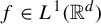 $f\in L^1(\mathbb {R}^d)$
with compact support, we define the variation of f as
$f\in L^1(\mathbb {R}^d)$
with compact support, we define the variation of f as
 $$ \begin{align*}V(f)=\sup\bigg\{\!\int_{\mathbb{R}^d}f\text{div}(g)\,dm:g\in C_0^1(\mathbb{R}^d,\mathbb{R}^d) \text{ and } \|g\|\leq 1\bigg\},\end{align*} $$
where $C_0^1(\mathbb {R}^d,\mathbb {R}^d)$
is the set of
$C_0^1(\mathbb {R}^d,\mathbb {R}^d)$
is the set of $C^1$
functions from
$C^1$
functions from $\mathbb {R}^d$
to
$\mathbb {R}^d$
to $\mathbb {R}^d$
with compact support,
$\mathbb {R}^d$
with compact support, $\text {div}(g)$
is the divergence of g and
$\text {div}(g)$
is the divergence of g and $\|\quad \|$
is the sup norm in
$\|\quad \|$
is the sup norm in $C_0^1(\mathbb {R}^d,\mathbb {R}^d)$
. Integration by parts gives that if f is a
$C_0^1(\mathbb {R}^d,\mathbb {R}^d)$
. Integration by parts gives that if f is a $C^1$
function with compact support, then
$C^1$
function with compact support, then
 $$ \begin{align} V(f)=\int_{\mathbb{R}^d}\|Df\|\,dm. \end{align} $$
We shall use the following properties of bounded variation functions whose proofs may be found in [Reference Giusti25], respectively in Remark 2.14, Theorem 1.17 and Theorem 1.28.
-
(B1) If
$f\in BV(\mathbb R^d)$
is zero outside a compact domain K whose boundary is Lipschitz continuous,
$f|_K$
is continuous and
$f|_{\operatorname {int} (K)}$
is
$C^1$
, then where
$$ \begin{align*}V(f)= \int_{\operatorname{int}(K)} \|Df\| \,dm + \int_{\partial K}|f|\, d \bar m , \end{align*} $$
$\bar m $
denotes the
$(d-1)$
-dimensional measure on
$\partial K$
.
-
(B2) Given
$f\in BV(\mathbb R^d)$
, there is a sequence
$(f_n)_n$
of
$C^\infty $
maps such that
$$ \begin{align*} \lim_{n\rightarrow\infty}\int|f-f_n|\,dm=0 \quad\text{and}\quad \lim_{n\rightarrow\infty}\int\|Df_n\|\,dm=V(f). \end{align*} $$
-
(B3) There is some constant
$C>0$
such that, for any
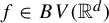
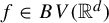
$f\in BV(\mathbb R^d)$
, (2.2)
$$ \begin{align} \bigg(\!\int|f|^pdm\bigg)^{1/p}\leq C\,V(f) \quad \text{with } p=\frac{d}{d-1}. \end{align} $$




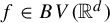

This last property is known as the Sobolev inequality. Notice that $p=d/(d-1)$
is the conjugate of
$p=d/(d-1)$
is the conjugate of $d\ge 1$
, meaning that
$d\ge 1$
, meaning that
 $$ \begin{align} \frac1p+\frac1d=1. \end{align} $$
In the next lemma, we obtain a general fact about bounded variation functions that plays a key role in this work.
Lemma 2.1. If K is a compact subset of $\mathbb R^d$
and
$\mathbb R^d$
and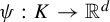 $\psi :K\to \mathbb {R}^d$
is a diffeomorphism onto its image, then there exists
$\psi :K\to \mathbb {R}^d$
is a diffeomorphism onto its image, then there exists $C>0$
such that, for all
$C>0$
such that, for all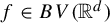 $f\in BV(\mathbb R^d)$
,
$f\in BV(\mathbb R^d)$
,
 $$ \begin{align*}\int_K|f\circ\psi-f|\,dm\le C\|\psi-\operatorname{id}\!\|_0 V(f). \end{align*} $$
Proof. We start by proving the result for a continuous piecewise affine function f. More precisely, suppose that the support $\Delta $
of f can be decomposed into a finite number of domains
$\Delta $
of f can be decomposed into a finite number of domains $\Delta _1,\ldots ,\Delta _N$
such that the gradient
$\Delta _1,\ldots ,\Delta _N$
such that the gradient $\nabla f$
of f is a constant vector
$\nabla f$
of f is a constant vector $\nabla _i f$
on each
$\nabla _i f$
on each $\Delta _i$
. Using property (B1), we obtain
$\Delta _i$
. Using property (B1), we obtain
 $$ \begin{align*} \int_K|f\circ \psi-f|\,dm\leq \int_K \|\psi-\operatorname{id}\!\|_0\cdot\|\nabla f\| \,dm \le \|\psi-\operatorname{id}\!\|_0 V(f). \end{align*} $$
The next step is to deduce the result for any $C^1$
function f. For this, we take a sequence
$C^1$
function f. For this, we take a sequence $(f_n)_n$
of continuous piecewise affine functions such that
$(f_n)_n$
of continuous piecewise affine functions such that
 $$ \begin{align*} \|f-f_n\|_0\rightarrow 0\quad\text{and}\quad \|Df-Df_n\|_0\rightarrow 0 \quad\text{when } n\rightarrow\infty \end{align*} $$
(the derivatives $Df_n$
are defined only in the interior of the smoothness domains). Then, using equation (2.1) and dominated convergence theorem, we have
$Df_n$
are defined only in the interior of the smoothness domains). Then, using equation (2.1) and dominated convergence theorem, we have
 $$ \begin{align*} V(f)=\int\|Df\|\,dm=\lim_{n\rightarrow\infty}\int\|Df_n\|\,dm =\lim_{n\rightarrow\infty}V(f_n) \end{align*} $$
and
 $$ \begin{align*} \int_K|f\circ\psi-f|\,dm=\lim_{n\rightarrow\infty} \int_K|f_n\circ\psi-f_n|\,dm. \end{align*} $$
Using the case already seen, we get the conclusion also for f.
For the general case, we know by property (B2) that given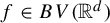 $f\in BV(\mathbb R^d)$
, there is a sequence
$f\in BV(\mathbb R^d)$
, there is a sequence $(f_n)_n$
of
$(f_n)_n$
of $C^1$
maps for which
$C^1$
maps for which
 $$ \begin{align} \lim_{n\rightarrow\infty}\int|f-f_n|\,dm=0 \quad\text{and}\quad \lim_{n\rightarrow\infty}V(f_n)=V(f). \end{align} $$
We have
 $$ \begin{align*} \int_K\! |f\circ\psi-f|\,dm\leq\!\int_K\! |f\circ\psi-f_n\circ\psi|\,dm +\!\int_K\! |f_n\circ\psi-f_n|\,dm +\!\int_K\! |f_n-f|\,dm. \end{align*} $$
Taking $\rho =1/|\!\det D\psi |\circ \psi ^{-1}$
, we may write
$\rho =1/|\!\det D\psi |\circ \psi ^{-1}$
, we may write
 $$ \begin{align*} \int_K|f_n\circ \psi-f\circ\psi|\,dm=\int_{\psi(K)}|f_n-f|\cdot \rho \,dm \leq \|\rho\|_0\int|f_n-f|\,dm. \end{align*} $$
The conclusion in this case follows from equation (2.4) and the previous case.
3 Transfer operators
Let $\Omega \subset \mathbb {R}^d$
be the common domain of the maps in the family
$\Omega \subset \mathbb {R}^d$
be the common domain of the maps in the family $\{\phi _t\}_{t\in I}$
. For each
$\{\phi _t\}_{t\in I}$
. For each $t\in I$
, consider the transfer operator
$t\in I$
, consider the transfer operator
 $$ \begin{align*}\mathcal{L}_t:L^1(\Omega)\longrightarrow L^1(\Omega),\end{align*} $$
defined for each $f\in L^1(\Omega )$
by
$f\in L^1(\Omega )$
by
 $$ \begin{align*}\mathcal{L}_t f=\sum_{i=1}^{N}\frac{f\circ\phi_{t,i}^{-1}}{J_t\circ\phi_{t,i}^{-1}} \chi_{\phi_t(R_{t,i})},\end{align*} $$
where $\{R_{t,i}\}_{i=1}^N$
are the domains of smoothness of
$\{R_{t,i}\}_{i=1}^N$
are the domains of smoothness of $\phi _t:\Omega \to \Omega $
and
$\phi _t:\Omega \to \Omega $
and $\phi _{t,i}$
are the maps introduced in equation (1.1). It is well known that the following properties hold for each
$\phi _{t,i}$
are the maps introduced in equation (1.1). It is well known that the following properties hold for each $\mathcal {L}_t$
:
$\mathcal {L}_t$
:
-
(C1) for all
$f,g$
for which the integrals make sense, we have
$$ \begin{align*}\int_\Omega f\mathcal{L}_t g \,dm =\int_\Omega f\circ \phi_t\, g\, dm;\end{align*} $$
-
(C2)
$|\mathcal {L}_t f|\le \mathcal {L}_t(|f|)$
and
$\|\mathcal {L}_t f\|_1\leq \| f\|_1$
for all
$f\in L^1(\Omega )$
; -
(C3)
$f \in L^1(\Omega ) $
is the density of an absolutely continuous
$\phi _t$
-invariant measure if and only if
$f \ge 0$
and
$\mathcal {L}_t f=f$
.






Next, we study the action of the transfer operators on the space of bounded variation functions in $\Omega $
,
$\Omega $
,
 $$ \begin{align*}BV(\Omega)=\{ f\in L^1(\Omega):V(f)<+\infty\}.\end{align*} $$
Property (B3) gives in particular $BV(\Omega )\subset L^p(\Omega )$
for some
$BV(\Omega )\subset L^p(\Omega )$
for some $p>1$
. Set for each
$p>1$
. Set for each $f\in BV(\Omega )$
,
$f\in BV(\Omega )$
,
 $$ \begin{align*} \|f\|_{BV}=\|f\|_1+V(f). \end{align*} $$
It is well known that this defines a norm and $BV(\Omega )$
endowed with this norm becomes a Banach space; see e.g. [Reference Giusti25, Remark 1.12].
$BV(\Omega )$
endowed with this norm becomes a Banach space; see e.g. [Reference Giusti25, Remark 1.12].
Proposition 3.1. Under assumption (U), there exist $0<\unicode{x3bb} <1$
and
$0<\unicode{x3bb} <1$
and $C>0$
such that, for all
$C>0$
such that, for all $t\in I$
,
$t\in I$
, $f\in BV(\Omega )$
and
$f\in BV(\Omega )$
and $n\ge 1$
, we have
$n\ge 1$
, we have
 $$ \begin{align*}\|\mathcal{L}_t^n f\|_{BV}\le C \unicode{x3bb}^n\|f\|_{BV}+ C \|f\|_1.\end{align*} $$
Proof. Take $\ell \ge 1$
as in assumption (U). It is a standard fact that
$\ell \ge 1$
as in assumption (U). It is a standard fact that $\mathcal {L}_t^\ell $
is the transfer operator for
$\mathcal {L}_t^\ell $
is the transfer operator for $\phi _t^\ell $
. By [Reference Alves1, Lemma 5.4], we have for any
$\phi _t^\ell $
. By [Reference Alves1, Lemma 5.4], we have for any $f\in BV(\Omega )$
,
$f\in BV(\Omega )$
,
 $$ \begin{align} V(\mathcal L^\ell_t f)\le \sigma_{t,\ell}\bigg(1+\frac1{\beta_{t,\ell}}\bigg)V(f)+M\|f\|_1\le \theta V(f)+ M \|f\|_1, \end{align} $$
and so
 $$ \begin{align} \|\mathcal L^\ell_t f\|_{BV}\le \theta V(f)+ (M+1) \|f\|_1. \end{align} $$
Given $n\ge 1$
, consider
$n\ge 1$
, consider $q\ge 0$
and
$q\ge 0$
and $0\le r<\ell $
such that
$0\le r<\ell $
such that $n=\ell q+r$
. It follows from property (C2) and equation (3.1) that
$n=\ell q+r$
. It follows from property (C2) and equation (3.1) that
 $$ \begin{align*} V(\mathcal L^{\ell q}_t f)&\le \theta V(\mathcal L^{\ell (q-1)}_t f)+M \|f\|_1\\ &\le \theta^2 V(\mathcal L^{\ell (q-2)}_t f)+(\theta +1)M \|f\|_1\\ &\ \ \vdots& \\ &\le \theta^q V( f)+(\theta^{q-1}+\theta^{q-2}+\cdots +1)M \|f\|_1. \end{align*} $$
It follows that
 $$ \begin{align} \|\mathcal{L}_t^{\ell q} f\|_{BV}=V(\mathcal{L}_t^{\ell q} f)+\|\mathcal{L}_t^{\ell q} f\|_1\le \theta^{q}V(f)+ \bigg(1+M\sum_{j\ge0}\theta^j\bigg) \|f\|_1. \end{align} $$
However,
 $$ \begin{align} V(\mathcal L^r_t f)\le \sigma_{t,r}\bigg(1+\frac1{\beta_{t,r}}\bigg) V(f)+ M \|f\|_1\le M V(f)+ M \|f\|_1. \end{align} $$
Finally, using equations (3.3) and (3.4), we get
 $$ \begin{align*} \|\mathcal{L}_t^n f\|_{BV}&=\|\mathcal{L}_t^{ \ell q} \mathcal{L}_t^r f\|_{BV}\\ &=\theta ^q V(\mathcal{L}_t^r f)+ \bigg(1+M\sum_{j\ge0}\theta^j\bigg) \|f\|_1\\ &\le \theta ^q MV( f)+ \bigg(M+1+M\sum_{j\ge0}\theta^j\bigg) \|f\|_1. \end{align*} $$
Now, observe that
 $$ \begin{align*}\theta^q=\theta^{(n-r)/\ell} = (\theta^{1/\ell})^n \theta^{-r/\ell} \le (\theta^{1/\ell})^n \theta^{-1}. \end{align*} $$
Take
 $$ \begin{align*}\unicode{x3bb}=\theta^{1/\ell}\quad\text{and}\quad C=\max\bigg\{\frac M\theta, M+1+M\sum_{j\ge0}\theta^j\bigg\}\end{align*} $$
and recall that $V(f)\le \|f\|_{BV}$
.
$V(f)\le \|f\|_{BV}$
.
It follows from the previous result that $\mathcal {L}_t(BV(\Omega ))\subset BV(\Omega )$
. From here on, we consider
$\mathcal {L}_t(BV(\Omega ))\subset BV(\Omega )$
. From here on, we consider $\mathcal {L}_t$
as an operator from the space
$\mathcal {L}_t$
as an operator from the space $BV(\Omega )$
into itself.
$BV(\Omega )$
into itself.
Proposition 3.2. Under the assumptions of Theorem A, there exists $C>0$
such that, for all
$C>0$
such that, for all $f\in BV(\Omega )$
,
$f\in BV(\Omega )$
,
 $$ \begin{align*}\|\mathcal{L}_t f-\mathcal{L}_s f\|_1\le C \mathcal E(t-s) \|f\|_{BV}\!.\end{align*} $$
Proof. Given $f\in BV(\Omega )$
, we have
$f\in BV(\Omega )$
, we have
 $$ \begin{align*} \|\mathcal{L}_t f-\mathcal{L}_s f\|_1\le C \mathcal E(t-s) \|f\|_{BV}\!. \end{align*} $$
Indeed,
 $$ \begin{align*} &\|\mathcal{L}_t f-\mathcal{L}_s f\|_1\\&\quad\le \sum_{i=1}^N\int_{\Omega} \bigg|\frac{f\circ\phi_{t,i}^{-1}}{J_t\circ\phi_{t,i}^{-1}} \chi_{\phi_t(R_{t,i})}-\frac{f\circ\phi_{s,i}^{-1}}{J_s\circ\phi_{s,i}^{-1}} \chi_{\phi_s(R_{s,i})}\bigg|\,dm\\ &\quad=\underbrace{\sum_{i=1}^N\int_{\phi_t(R_{t,i})\cap\phi_s(R_{s,i})} \bigg|\frac{f\circ\phi_{t,i}^{-1}}{J_t\circ\phi_{t,i}^{-1}}- \frac{f\circ\phi_{s,i}^{-1}}{J_s\circ\phi_{s,i}^{-1}} \bigg|\,dm}_{\text{(I)}}\\ &\qquad+ \underbrace{\sum_{i=1}^N\int_{\phi_t(R_{t,i})\setminus\phi_s(R_{s,i})} \bigg|\frac{f\circ\phi_{t,i}^{-1}}{J_t\circ\phi_{t,i}^{-1}}\bigg|\,dm}_{\text{(II)}} + \underbrace{\sum_{i=1}^N\int_{\phi_s(R_{s,i})\setminus\phi_t(R_{t,i})} \bigg|\frac{f\circ\phi_{s,i}^{-1}}{J_s\circ\phi_{s,i}^{-1}} \bigg|\,dm}_{\text{(III)}}. \end{align*} $$
We just need to obtain the appropriate bounds for parts (I), (II) and (III). To estimate part (I), note that by the change of variables $y=\phi _{s,i}(x)$
, we have
$y=\phi _{s,i}(x)$
, we have
 $$ \begin{align*} &\int_{\phi_t(R_{t,i})\cap\phi_s(R_{s,i})} \bigg|\frac{f\circ\phi_{t,i}^{-1}}{J_t\circ\phi_{t,i}^{-1}}-\frac{f\circ\phi_{s,i}^{-1}}{J_s\circ\phi_{s,i}^{-1}}\bigg|\,dm\\ &\quad=\int_{\phi_{s,i}^{-1}(\phi_t(R_{t,i})\cap\phi_s(R_{s,i}))} \bigg|\frac{f\circ\phi_{t,i}^{-1}\circ \phi_{s,i}} {J_t\circ\phi_{t,i}^{-1}\circ \phi_{s,i}}-\frac{f}{J_s}\bigg|J_s\,dm. \end{align*} $$
Set $\psi _{t,s,i}=\phi _{t,i}^{-1}\circ \phi _{s,i}|_{\phi _{s,i}^{-1}(\phi _t(R_{t,i})\cap \phi _s(R_{s,i}))}$
. Therefore,
$\psi _{t,s,i}=\phi _{t,i}^{-1}\circ \phi _{s,i}|_{\phi _{s,i}^{-1}(\phi _t(R_{t,i})\cap \phi _s(R_{s,i}))}$
. Therefore,
 $$ \begin{align*} \text{(I)} &= \sum_{i=1}^N\int_{K_{t,s,i}} \bigg|\frac{f\circ\phi_{t,i}^{-1}\circ \phi_{s,i}} {J_t\circ\phi_{t,i}^{-1}\circ \phi_{s,i}}-\frac{f}{J_s}\bigg|J_s\,dm\\ &\le \sum_{i=1}^N\int_{K_{t,s,i}} |f\circ\psi_{t,s,i}-f|\bigg|\frac{J_s}{J_t\circ\psi_{t,s,i}}\bigg|\,dm + \sum_{i=1}^N\int_{K_{t,s,i}} \bigg|\frac{J_s}{J_t\circ\psi_{t,s,i}}-1\bigg||f|\,dm. \end{align*} $$
By assumption (3) of Theorem A, there exists some $C_0>0$
such that, for each
$C_0>0$
such that, for each $1\le i<N$
,
$1\le i<N$
,
 $$ \begin{align*} \bigg|\frac{J_s}{J_t\circ\psi_{t,s,i}}\bigg| \le 1+\sup_{1\le i<N} \bigg|\frac{J_s}{J_t\circ\psi_{t,s,i}}-1\bigg| \le 1+ \sum_{i=1}^N \bigg|\frac{J_s}{J_t\circ\psi_{t,s,i}}-1\bigg| \le C_0. \end{align*} $$
By Lemma 2.1 and the assumptions of Theorem A, we may write
 $$ \begin{align*} \text{(I)} &\le C_0 \sum_{i=1}^N\|\psi_{t,s,i}-\operatorname{id}\!\|_0\, V(f)+\sum_{i=1}^N \bigg|\frac{J_s}{J_t\circ\psi_{t,s,i}}-1\bigg|\|f\|_1\\ &\le C\mathcal E(t-s)\|f\|_{BV} \end{align*} $$
for some uniform constant $C>0$
. To estimate part (II), note that, by change of variables,
$C>0$
. To estimate part (II), note that, by change of variables,
 $$ \begin{align*} \int_{\phi_t(R_{t,i})\setminus\phi_s(R_{s,i})} \bigg|\frac{f\circ\phi_{t,i}^{-1}}{J_t\circ\phi_{t,i}^{-1}}\bigg|\,dm &= \int_{\phi_{t,i}^{-1}(\phi_t(R_{t,i})\setminus\phi_s(R_{s,i}))} |f| \,dm\\ &= \int_\Omega \chi_{\phi_{t,i}^{-1}(\phi_t(R_{t,i})\setminus\phi_s(R_{s,i}))} | f |\,dm. \end{align*} $$
Observe that, by the Sobolev inequality (B3), we have $f\in L^p(\Omega )$
, with
$f\in L^p(\Omega )$
, with $p=d/(d-1)$
and d being conjugate. It follows from Hölder and Sobolev inequalities and assumption (1) of Theorem A that there exists some
$p=d/(d-1)$
and d being conjugate. It follows from Hölder and Sobolev inequalities and assumption (1) of Theorem A that there exists some $C>0$
such that
$C>0$
such that
 $$ \begin{align*} \text{(II)}&= \sum_{i=1}^N\int_\Omega \chi_{\phi_{t,i}^{-1}(\phi_t(R_{t,i})\setminus\phi_s(R_{s,i}))} | f |\,dm\\ &\le\sum_{i=1}^N\|\chi_{\phi_{t,i}^{-1}(\phi_t(R_{t,i})\setminus\phi_s(R_{s,i}))}\|_d\|f\|_p\\ &\le C \sum_{i=1}^N m(\phi_{t,i}^{-1}(\phi_t(R_{t,i})\setminus\phi_s(R_{s,i})))^{1/d}\|f\|_{BV}\\ &\le C\mathcal E(t-s) \|f\|_{BV}. \end{align*} $$
We are done for part (II). The calculations follow similarly for part (III).
4 Modulus of continuity for the densities
In this section, we prove Theorem A. We will use a Galatolo–Lucena stability result presented in [Reference Galatolo and Lucena24] for uniform families of operators as in [Reference Galatolo and Lucena24, Definition 9.1] described below in conditions (UF1)–(UF4). First, notice that 1 is an isolated eigenvalue, by the theorem of Ionescu Tulcea and Marinescu [Reference Ionescu Tulcea and Marinescu27], since $\mathcal {L}_t$
is quasicompact; moreover, it has multiplicity one, because we assume that each
$\mathcal {L}_t$
is quasicompact; moreover, it has multiplicity one, because we assume that each $\phi _t $
has a unique ergodic absolutely continuous invariant probability measure; recall property (C3). Let
$\phi _t $
has a unique ergodic absolutely continuous invariant probability measure; recall property (C3). Let $\rho _t \in BV(\Omega )$
denote the density of that measure. We need to show that there exist
$\rho _t \in BV(\Omega )$
denote the density of that measure. We need to show that there exist $C>0$
and
$C>0$
and $0<r<1$
such that, for all
$0<r<1$
such that, for all $t,s\in I$
:
$t,s\in I$
:
-
(UF1)
$\|\rho _t\|_{BV}\le C $
; -
(UF2)
$\|(\mathcal {L}_t-\mathcal {L}_s)\rho _t\|_1\le C\mathcal E(t-s) $
; -
(UF3)
$\|\mathcal {L}_t^nf\|_1\le Cr^n\|f\|_{BV}$
for all
$f\in BV(\Omega )$
with
$\int f \,dm=0$
and
$n\ge 1$
; -
(UF4)
$\|\mathcal {L}_t^n f\|_1\le C \|f\|_1$
for all
$f\in BV(\Omega )$
and
$n\ge 1$
.




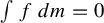




Let us now justify that these conditions are satisfied. In fact, it follows from Proposition 3.1 that, for all $n\ge 1$
,
$n\ge 1$
,
 $$ \begin{align*}\|\mathcal{L}_t^n f\|_{BV}\le C\unicode{x3bb}^n\|f\|_{BV}+ C \|f\|_1\end{align*} $$
for all $f\in BV(\Omega )$
and
$f\in BV(\Omega )$
and $t\in I$
. Since
$t\in I$
. Since $\rho _t$
is the fixed point for
$\rho _t$
is the fixed point for $\mathcal {L}_t$
with
$\mathcal {L}_t$
with $\|\rho _t\|_1=1$
and the last inequality holds for all
$\|\rho _t\|_1=1$
and the last inequality holds for all $n\ge 1$
, we get condition (UF1). Then, condition (UF2) follows from Proposition 3.2 and condition (UF1). Now, it follows from [Reference Rychlik39, Theorem 3] that, for all
$n\ge 1$
, we get condition (UF1). Then, condition (UF2) follows from Proposition 3.2 and condition (UF1). Now, it follows from [Reference Rychlik39, Theorem 3] that, for all $t \in I$
and
$t \in I$
and $f \in L^1(\Omega )$
, we have
$f \in L^1(\Omega )$
, we have
 $$ \begin{align*} \Pi_t f = \rho_t \int f \,dm,\end{align*} $$
where $\Pi _t$
is the projection onto the eigenspace of the eigenvalue 1 with respect to the operators
$\Pi _t$
is the projection onto the eigenspace of the eigenvalue 1 with respect to the operators $\mathcal {L}_t$
. Observing that
$\mathcal {L}_t$
. Observing that $\Pi _t f=0$
for all
$\Pi _t f=0$
for all $f \in L^1(\Omega )$
with
$f \in L^1(\Omega )$
with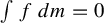 $\int f \,dm=0$
, condition (UF3) is a consequence of [Reference Rychlik39, Theorem 1]. Finally, condition (UF4) follows easily from property (C3) in §3.
$\int f \,dm=0$
, condition (UF3) is a consequence of [Reference Rychlik39, Theorem 1]. Finally, condition (UF4) follows easily from property (C3) in §3.
The conclusion of Theorem A then follows from [Reference Galatolo and Lucena24, Proposition 32].
Remark 4.1. The considerations in the beginning of this section, together with Proposition 3.1 and Proposition 3.2, show that we are in the setting of the Keller–Liverani stability result. This enables us to obtain a quantitative estimate on the continuity of the resolvents associated with the transfer operators for our family of maps. Specifically, it follows from [Reference Keller and Liverani30, Theorem 1] that, fixing $\delta>0$
,
$\delta>0$
, $r\in (\unicode{x3bb} ,1)$
and
$r\in (\unicode{x3bb} ,1)$
and $\eta =\log (r/\unicode{x3bb} )/\log (1/\unicode{x3bb} )$
(with
$\eta =\log (r/\unicode{x3bb} )/\log (1/\unicode{x3bb} )$
(with ${0<\unicode{x3bb} <1}$
given by Proposition 3.1), there are constants
${0<\unicode{x3bb} <1}$
given by Proposition 3.1), there are constants $a,b,c,d>0$
such that for any
$a,b,c,d>0$
such that for any $z\in \mathbb C$
with
$z\in \mathbb C$
with
 $$ \begin{align*}|z|>r \quad\text{and}\quad \operatorname{dist}(z,\sigma(\mathcal{L}_s))>\delta,\end{align*} $$
where $\sigma (\mathcal {L}_s)$
is the spectrum of
$\sigma (\mathcal {L}_s)$
is the spectrum of $\mathcal {L}_s$
, we have for all
$\mathcal {L}_s$
, we have for all $f\in BV(\Omega )$
:
$f\in BV(\Omega )$
:
-
(1)
$\|(z-\mathcal {L}_t)^{-1}f\|_{BV}\le a\|f\|_{BV}+b\|f\|_1$
; -
(2)
${\vert \kern -0.25ex\vert \kern -0.25ex\vert (z-\mathcal {L}_t)^{-1}-(z-\mathcal {L}_s)^{-1} \vert \kern -0.25ex\vert \kern -0.25ex\vert }\le \mathcal E(t-s)^\eta (c\|(z-\mathcal {L}_s)^{-1}\|_{BV}+d \|(z-\mathcal {L}_s)^{-1}\|_{BV}^2), $


where ${\vert \kern -0.25ex\vert \kern -0.25ex\vert \quad \vert \kern -0.25ex\vert \kern -0.25ex\vert }$
is defined for an operator
${\vert \kern -0.25ex\vert \kern -0.25ex\vert \quad \vert \kern -0.25ex\vert \kern -0.25ex\vert }$
is defined for an operator $T:BV(\Omega )\to BV(\Omega )$
by
$T:BV(\Omega )\to BV(\Omega )$
by
 $$ \begin{align*}{\vert\kern-0.25ex\vert\kern-0.25ex\vert T \vert\kern-0.25ex\vert\kern-0.25ex\vert}= \sup_{\{f \in BV(\Omega) : \| f \|_{BV} \leq 1 \}} \|T f \|_1.\end{align*} $$
5 Modulus of continuity for the entropies
Here, we prove Theorem B. For each $t\in I$
, let
$t\in I$
, let $\rho _t$
denote the density of
$\rho _t$
denote the density of $\mu _t$
with respect to m. Since the entropy formula in assumption (2) holds, we have for all
$\mu _t$
with respect to m. Since the entropy formula in assumption (2) holds, we have for all $s,t\in I$
,
$s,t\in I$
,
 $$ \begin{align*} |h_{\mu_s}(\phi_s)-h_{\mu_t}(\phi_t)|&= \bigg|\! \int\log J_s\,d\mu_s-\int\log J_t\, d\mu_t\bigg|\\ &\le \bigg|\! \int(\log J_s-\log J_t )\,d\mu_s\bigg|+ \bigg|\! \int\log J_t\,d\mu_s-\int\log J_t\, d\mu_t\bigg|\\ &\le \bigg|\! \int(\log J_s- \log J_t )\rho_s \,dm\bigg|+ \bigg|\! \int\log J_t(\rho_s-\rho_t)\,dm\bigg|. \end{align*} $$
Using Hölder inequality and the bound in assumption (2), we get
 $$ \begin{align} \bigg|\! \int\log J_t(\rho_s-\rho_t)\,dm\bigg|\le M\|\rho_s-\rho_t\|_1. \end{align} $$
However, condition (UF1) gives that $ \|\rho _s\|_{BV}\le C. $
Taking
$ \|\rho _s\|_{BV}\le C. $
Taking $p=d/(d-1)$
, it follows from Sobolev inequality that there exists a constant
$p=d/(d-1)$
, it follows from Sobolev inequality that there exists a constant $C'>0$
such that
$C'>0$
such that
 $$ \begin{align} \|\rho_s\|_p\le C'. \end{align} $$
Hence, using Hölder inequality and equation (5.2), we get
 $$ \begin{align} \bigg|\! \int (\kern-1.2pt\log J_s - \log J_t )\rho_s \,dm\bigg|\le \|\rho_s\|_p \|\!\log J_s - \log J_t\|_d\le C'\|\!\log J_s- \log J_t\|_d. \end{align} $$
The conclusion follows from equations (5.1), (5.3) and assumption (1) of Theorem B.
6 Application to tent maps
Here, we prove Theorem C. Our strategy is to apply Theorems A and B to the family of tent maps $(\phi _t)_{t \in [\tau ,1]}$
presented in §1.2. We know that
$(\phi _t)_{t \in [\tau ,1]}$
presented in §1.2. We know that $R_1$
and
$R_1$
and $R_2$
are the only domains of smoothness of every
$R_2$
are the only domains of smoothness of every $\phi _t$
. Therefore, for each
$\phi _t$
. Therefore, for each $t\in [\tau ,1]$
and
$t\in [\tau ,1]$
and $i=1,2$
, we have
$i=1,2$
, we have
 $$ \begin{align*}\phi_{t,i}=\phi_t|_{R_{i}},\quad K_{t,s,i}=\phi_{s,i}^{-1}(\phi_t(R_{i})\cap\phi_s(R_{i}))\quad\text{and}\quad \psi_{t,s,i}=\phi_{t,i}^{-1}\circ \phi_{s,i}|_{K_{t,s,i}} .\end{align*} $$
According to [Reference Alves, Pumariño and Vigil8, §4], the uniformity condition (U) is satisfied with $\ell =6$
. Existence and uniqueness of an ergodic absolutely continuous
$\ell =6$
. Existence and uniqueness of an ergodic absolutely continuous $\phi _t$
-invariant probability measure
$\phi _t$
-invariant probability measure $\mu _t$
was obtained in [Reference Pumariño, Rodríguez, Tatjer and Vigil36] for all
$\mu _t$
was obtained in [Reference Pumariño, Rodríguez, Tatjer and Vigil36] for all $t \in [\tau ,1]$
. Moreover, the entropy formula holds for this family of maps, by [Reference Alves and Pumariño9, Theorem G]. We are left to verify the assumptions of Theorems A and B with adequate estimates to deduce Theorem C. It is enough to show that there exists some constant
$t \in [\tau ,1]$
. Moreover, the entropy formula holds for this family of maps, by [Reference Alves and Pumariño9, Theorem G]. We are left to verify the assumptions of Theorems A and B with adequate estimates to deduce Theorem C. It is enough to show that there exists some constant $M>0$
such that, for all
$M>0$
such that, for all $s,t\in [\tau ,1]$
and
$s,t\in [\tau ,1]$
and $i=1,2$
, we have:
$i=1,2$
, we have:
-
(a)
$ m(\phi _{t,i}^{-1}(\phi _t(R_{i})\setminus \phi _s(R_{i}))) \le M |t-s|;$
-
(b)
$ \|\psi _{t,s,i}-\operatorname {id}\!\|_0 \le M |t-s|;$
-
(c)
$ |{J_s}/({J_t\circ \psi _{t,s,i}}) -1 |\le M |t-s|;$
-
(d)
$\|\!\log {J_s}-\log {J_t}\|_d\le M |t-s|;$
-
(e)
$\|\!\log J_t\|_\infty \le M.$





Indeed, from equation (1.2), we easily deduce that, for all $(y_1,y_2)\in \phi _{t,1}(R_1)$
, we have
$(y_1,y_2)\in \phi _{t,1}(R_1)$
, we have
 $$ \begin{align*} \phi_{t,1}^{-1}(y_1,y_2)=\bigg(\frac{1}{2t}(y_1+y_2),\frac{1}{2t}(y_1-y_2)\bigg) \end{align*} $$
and, for all $(y_1,y_2)\in \phi _{t,2}(R_2)$
, we have
$(y_1,y_2)\in \phi _{t,2}(R_2)$
, we have
 $$ \begin{align*} \phi_{t,2}^{-1}(y_1,y_2)=\bigg(\frac{1}{2t}(4t-y_1-y_2),\frac{1}{2t}(y_1-y_2)\bigg). \end{align*} $$
Moreover, each map $\phi _t$
is piecewise linear with
$\phi _t$
is piecewise linear with
 $$ \begin{align*} D\phi_t(x_1, x_2)= \left(\! \begin{array}{cc} t & t \\ t & -t \end{array}\!\right) \end{align*} $$
for all $(x_1, x_2)\in R_1\setminus \mathcal C$
, and
$(x_1, x_2)\in R_1\setminus \mathcal C$
, and
 $$ \begin{align*} D\phi_t(x_1, x_2)= \left(\! \begin{array}{cc} - t & t \\ - t & -t \end{array}\!\right) \end{align*} $$
for all $(x_1, x_2)\in R_2\setminus \mathcal C$
. Therefore, we have
$(x_1, x_2)\in R_2\setminus \mathcal C$
. Therefore, we have
 $$ \begin{align*}J_t=2t^2\end{align*} $$
for all $(x_1, x_2)\in \Omega \setminus \mathcal C$
and
$(x_1, x_2)\in \Omega \setminus \mathcal C$
and $\tau \le t\le 1$
.
$\tau \le t\le 1$
.
Proof of property (a)
Observe from the dynamics of $\phi _t$
that
$\phi _t$
that $\phi _{t,1}(R_1)=\phi _{t,2}(R_2)$
and, moreover, the Jacobian of
$\phi _{t,1}(R_1)=\phi _{t,2}(R_2)$
and, moreover, the Jacobian of $\phi _{t,1}$
is constant and equal to the Jacobian of
$\phi _{t,1}$
is constant and equal to the Jacobian of $\phi _{t,2}$
. Therefore, it is enough to show the conclusion for
$\phi _{t,2}$
. Therefore, it is enough to show the conclusion for $i=1$
. In fact, for
$i=1$
. In fact, for $t>s$
(and for
$t>s$
(and for $t<s$
, there is nothing to be proved, since in that case,
$t<s$
, there is nothing to be proved, since in that case, $\phi _t(R_1)\subset \phi _s(R_1)$
), we have
$\phi _t(R_1)\subset \phi _s(R_1)$
), we have
 $$ \begin{align} m(\phi_{t}(R_1)\setminus \phi_{s}(R_1)) &\le\text{length } (\phi_t(\mathcal{C}))\,\| \phi_t(1,0)-\phi_s(1,0)\|\nonumber \\ &= \sqrt{2}t \Vert (t,t)-(s,s) \Vert = 2t(t-s). \end{align} $$
Since the Jacobian of $\phi _{t,1}$
is constant and equal to
$\phi _{t,1}$
is constant and equal to $2t^2 $
, we deduce that the Jacobian of
$2t^2 $
, we deduce that the Jacobian of $\phi _{t,1}^{-1}$
is
$\phi _{t,1}^{-1}$
is $1/(2t^2) $
, which together with equation (6.1) yields
$1/(2t^2) $
, which together with equation (6.1) yields
 $$ \begin{align*} m(\phi_{t,i}^{-1}(\phi_t(R_{i})\setminus\phi_s(R_{i}))) \le \frac{(t-s)}{t} \le \frac{(t-s)}{\tau}.\\[-42pt] \end{align*} $$
Proof of property (b)
For each $(x_1,x_2) \in R_1$
and
$(x_1,x_2) \in R_1$
and $\tau \le t\le 1$
, we have
$\tau \le t\le 1$
, we have
 $$ \begin{align*} \|\psi_{t,s,i}-\operatorname{id}\!\|_0 &= \sup_{(x_1,x_2) \in R_1} \|\phi_{t,1}^{-1}\circ \phi_{s,1}(x_1,x_2)-(x_1,x_2)\|\\ &=\sup_{(x_1,x_2) \in R_1}\bigg\|\bigg(\frac{s}{t}-1\bigg)(x_1,x_2)\bigg\|\\ &\le \frac{\sqrt{2}}{\tau} |{t-s}|, \end{align*} $$
and for each $(x_1,x_2)\in R_2$
, we have
$(x_1,x_2)\in R_2$
, we have
 $$ \begin{align*} \|\psi_{t,s,i}-\operatorname{id}\!\|_0&= \sup_{(x_1,x_2) \in R_2} \|\phi_{t,2}^{-1}\circ \phi_{s,2}(x_1,x_2)-(x_1,x_2)\|\\ &= \sup_{(x_1,x_2) \in R_2}\bigg \|\bigg(\frac{s}{t}-1\bigg)\bigg(x_1-2, x_2 \bigg) \bigg \|\\ &\le \frac{\sqrt{2}}{\tau} |{t-s}|.\\[-40pt] \end{align*} $$
Proof of property (c)
For all $\tau \le s,t\le 1$
, we have
$\tau \le s,t\le 1$
, we have
 $$ \begin{align*} \bigg|\frac{J_s }{J_t\circ \psi_{t,s,i}}-1\bigg|= \bigg|\frac{s^2}{t^2}-1\bigg| = \bigg|\frac{(s-t)(s+t)}{t^2} \bigg|\le \frac{2}{\tau^2}|t-s|.\\[-42pt] \end{align*} $$
Proof of property (d)
By the mean value theorem, we have that for all $\tau \le s,t\le 1$
,
$\tau \le s,t\le 1$
,
 $$ \begin{align*} \|\!\log {J_s}-\log{J_t}\|_2=\bigg(\!\int_\Omega\bigg(\frac{2}{\tau}(s-t)\bigg)^2 \,dm\bigg)^{1/2} \le \frac2\tau m(\Omega) |t-s|.\\[-42pt] \end{align*} $$
Proof of property (e)
For all $\tau \le t\le 1$
, we have
$\tau \le t\le 1$
, we have
 $$ \begin{align*} \|\!\log J_t \|_\infty = |\kern-1.2pt \log (2t^2)|\le \log 2. \end{align*} $$
Recall that the expression for $\tau $
in equation (1.3) gives
$\tau $
in equation (1.3) gives $1<2\tau ^2\le 2t^2\le 2$
.
$1<2\tau ^2\le 2t^2\le 2$
.
Acknowledgements
The authors are grateful to Wael Bahsoun for several insightful discussions and careful reading of an early draft of this work. The authors also thank the anonymous referee for pointing out the possibility of improving the conclusion in Theorem A using [Reference Galatolo and Lucena24] instead of [Reference Keller and Liverani30]. J.F.A. and O.E. are partially supported by CMUP (UIDB/00144/2020) and PTDC/MAT-PUR/4048/2021, which are funded by FCT (Portugal) with national (MEC) and European structural funds through the programs COMPTE and FEDER, under the partnership agreement PT2020.




 Open access

