


1. Introduction
Industrial processes, such as those in chemical and nuclear power plants, often involve the intentional initiation of boiling or the injection of bubbles into a turbulent working fluid. The rationales for introducing a dispersed gaseous phase in practical applications are manifold and depend on the desired process enhancement.
For example, in steel-making operations, gas blowing promotes the circulation and homogenisation of molten steel, while simultaneously enhancing its cleanliness (Wang et al. Reference Wang, Cao, Vanierschot, Cheng, Blanpain and Guo2020; Yang et al. Reference Yang, Luo, Gu, Liu and Zou2020b ; Chang et al. Reference Chang, Zou, Liu, Isac, Cao, Su and Guthrie2021). Impurities can adhere to the bubble surfaces (Zhang & Taniguchi Reference Zhang and Taniguchi2000; Yang et al. Reference Yang, Xing, Sun, Cao and Gui2020a ) or become entrained in the bubble wakes (Söder et al. Reference Söder, Jönsson and Jonsson2004; Xu, Ersson & Jönsson Reference Xu, Ersson and Jönsson2016; Lou & Zhu Reference Lou and Zhu2016), facilitating their removal. However, the presence of small bubbles also poses challenges: they can become trapped in solidifying shells, leading to defects in the final cast material (Yang et al. Reference Yang, Luo, Gu, Liu and Zou2020b ).
Similarly, in biotechnological and pharmaceutical industries, fermentation processes rely on bubble spargers to supply oxygen needed by microorganisms for metabolite production (Gelves, Dietrich & Takors Reference Gelves, Dietrich and Takors2014; Niño et al. Reference Niño, Gelves and Solsvik2023). Successful aeration is dictated by multiple factors, such as bubble size distribution, bubble area distribution, mass transfer coefficient and bubble terminal velocity (Kure, Jakobsen & Solsvik Reference Kure, Jakobsen and Solsvik2024; Hosen et al. Reference Hosen, Shahmardi, Brandt and Solsvik2024).
Another important example arises in boiling water reactors, where heat removal enhancement is achieved through boiling processes (Silvi et al. Reference Silvi, Chandraker, Ghosh and Das2021; Roccon Reference Roccon2025). Initially, the cooling fluid enters the reactor core as a single-phase liquid and subsequently evaporates due to the heat transferred from the fuel rod walls. The nucleation and growth of bubbles require the absorption of latent heat, thereby extracting thermal energy from the surrounding hot liquid. Following detachment from the heated surfaces, the vacated volume is replenished by colder liquid, promoting local cooling. The detached bubbles then rise through the fluid due to buoyancy forces, enhancing vertical mixing and further contributing to heat removal (Lienhard IV & Lienhard V Reference Lienhard IV and Lienhard V2005; Lakkaraju et al. Reference Lakkaraju, Stevens, Oresta, Verzicco, Lohse and Prosperetti2013).
Despite the diversity of these applications, they share common underlying physical mechanisms: the introduction of a dispersed gaseous phase leads to highly complex flow phenomena (e.g. coalescence and breakage), primarily due to the action of buoyancy forces on the bubbles. Buoyancy not only governs the motion of the dispersed phase but also generates additional shear in the carrier liquid, modifying the local turbulence structure (Bunner & Tryggvason Reference Bunner and Tryggvason2003; Lu, Fernández & Tryggvason Reference Lu, Fernández and Tryggvason2005; Riboux, Risso & Legendre Reference Riboux, Risso and Legendre2010; Ravelet, Colin & Risso Reference Ravelet, Colin and Risso2011; Bolotnov Reference Bolotnov2013). However, a fundamental understanding of key local phenomena, such as the bubble wake dynamics and trajectory instabilities, remains limited. Historically, the simulation of turbulent multiphase flows was extremely challenging due to the demanding computational cost associated with resolving the wide range of spatial and temporal scales involved. As a result, early research efforts predominantly relied on experimental studies (Serizawa, Kataoka & Michiyoshi Reference Serizawa, Kataoka and Michiyoshi1975; Wang et al. Reference Wang, Lee, Jones and Lahey1987; Liu Reference Liu1993). In recent years, advancements in computational power and numerical methods have enabled the research community to increasingly focus on the detailed simulation of multiphase turbulent flows, providing new insights into previously inaccessible aspects of these systems (Santarelli, Roussel & Fröhlich Reference Santarelli, Roussel and Fröhlich2016; Lu & Tryggvason Reference Lu and Tryggvason2018; du Cluzeau, Bois & Toutant Reference du Cluzeau, Bois and Toutant2019; Lu & Tryggvason Reference Lu and Tryggvason2019; du Cluzeau et al. Reference du Cluzeau, Bois, Leoni and Toutant2022; Lee et al. Reference Lee, Chang, Kim and Choi2024; Lu, Yang & Deng Reference Lu, Yang and Deng2025). Most of these numerical studies have focused on the modulation of turbulence due to the dispersed phase, particularly in canonical configurations. In contrast, despite their central role in numerous industrial processes, significantly fewer efforts have been devoted to understanding how bubbles influence passive scalar transport or heat transfer.
Among the earliest studies in this direction, Tanaka (Reference Tanaka2011) investigated heat transfer in a turbulent vertical channel with bubble injection, without accounting for bubble break-up or coalescence. His findings indicated that heat transfer was enhanced relative to both single-phase flows and cases with neutrally buoyant droplets; however, this improvement was accompanied by increased wall-shear stress. These results suggest that the net benefit of bubbly flows for heat transport depends critically on the interplay between buoyancy-induced motion and frictional losses at the wall. Deen & Kuipers (Reference Deen and Kuipers2013) examined the behaviour of a single bubble and a few bubbles rising near a heated wall. They showed that the local heat-transfer coefficient peaks in the vicinity of the bubble due to thinning of the thermal boundary layer. Moreover, bubble-induced agitation significantly enhanced wall–liquid heat transfer, especially in regions where coalescence prevailed. Successively, Dabiri & Tryggvason (Reference Dabiri and Tryggvason2015) analysed heat transfer in a turbulent vertical channel flow laden with bubbles. They focused on the effect of the surface tension in the non-coalescing/breaking case. Their simulations demonstrated that the largest enhancement in heat transfer occurred at a low surface tension value. In particular, nearly spherical bubbles rising close to the walls disrupted the viscous sublayer and reduced the thickness of the conduction-dominated region, thereby increasing the heat-transfer rate. Similarly, Panda et al. (Reference Panda, Weitkamp, Rajkotwala, Peters, Baltussen and Kuipers2019) investigated the effect of the volume fraction, reporting a plateau in the global heat exchange enhancement. More recently, research has extended to the behaviour of passive scalars in homogeneous bubbly suspensions. Notably, Loisy, Naso & Spelt (Reference Loisy, Naso and Spelt2018) explored the convective contributions to effective scalar diffusivity, while Hidman et al. (Reference Hidman, Ström, Sasic and Sardina2023) provided physical interpretations of the observed $-3$
scaling in the scalar energy spectrum.
$-3$
scaling in the scalar energy spectrum.
From the experimental perspective, the seminal work of Deckwer (Reference Deckwer1980) investigated heat transfer in column bubble reactors, combining the surface renewal model (Kast Reference Kast1962) with Kolmogorov’s isotropic turbulent theory. Further studies highlighted the connection between the bubble-induced turbulence – composed of the induced liquid motion and the turbulence created in their wakes – and the heat-transfer enhancement both in liquid metals (Tokuhiro & Lykoudis Reference Tokuhiro and Lykoudis1994) and water (Kitagawa, Kitada & Hagiwara Reference Kitagawa, Kitada and Hagiwara2010; Kitagawa & Murai Reference Kitagawa and Murai2013; Kitagawa, Denissenko & Murai Reference Kitagawa, Denissenko and Murai2017). Subsequent works on homogeneous bubbly flows attested the predominance of the bubble-induced mixing over natural convection, modelling the mixing as a diffusion process (Alméras et al. Reference Alméras, Risso, Roig, Cazin, Plais and Augier2015; Gvozdić et al. Reference Gvozdić, Alméras, Mathai, Zhu, van Gils, Verzicco, Huisman, Sun and Lohse2018). Similarly to Hidman et al. (Reference Hidman, Ström, Sasic and Sardina2023), Dung et al. (Reference Dung, Waasdorp, Sun, Lohse and Huisman2023) examined the modification of the scalar spectrum of a turbulent flow due to bubble injection. They speculated that the transition from the $-5/3$
to
$-5/3$
to $-3$
scaling is mainly due to the enhanced homogenisation promoted by the dispersed phase, which reduces the small-scale temperature differences.
$-3$
scaling is mainly due to the enhanced homogenisation promoted by the dispersed phase, which reduces the small-scale temperature differences.
Although passive scalar transport has received attention, a comprehensive discussion of the combined effects of shear-induced and bubble-induced turbulence, which includes coalescence and breakage phenomena, on the heat transfer is still lacking. It is worth highlighting that topological changes might lead to very different volume fraction distributions with significant effects on turbulent modulation. In this study, we perform direct numerical simulations (DNS) of turbulent bubbly upflows in a vertical channel using a volume of fluid (VOF) method (Lee et al. Reference Lee, Chang, Kim and Choi2024; Lu et al. Reference Lu, Yang and Deng2025). Our goal is to investigate how a swarm of large, deformable bubbles alters the heat-transfer process across different thermal transport regimes. Specifically, we choose three different Prandtl numbers $\textit{Pr}=0.07,0.7$
and
$\textit{Pr}=0.07,0.7$
and $7.0$
(i.e. ratio of momentum-to-thermal diffusivity) representative of the thermal properties of liquid metals, vapour and water, respectively. To the extent of the authors’ knowledge, this is the first attempt to characterise heat-transfer modulation in a heterogeneous bubbly system across three orders of magnitude of
$7.0$
(i.e. ratio of momentum-to-thermal diffusivity) representative of the thermal properties of liquid metals, vapour and water, respectively. To the extent of the authors’ knowledge, this is the first attempt to characterise heat-transfer modulation in a heterogeneous bubbly system across three orders of magnitude of $\textit{Pr}$
, using DNS.
$\textit{Pr}$
, using DNS.
This paper is structured as follows. We begin in § 2 by outlining the governing equations and numerical methods. Section 3 then details the simulation set-up. The results are presented in § 4, where we first examine the qualitative behaviour before delving into the turbulence modifications driven by the bubbles and their effect on temperature statistics and heat transfer. Finally, § 5 provides a summary of the key findings and conclusions.
2. Governing equations
We employ DNS of the Navier–Stokes equations coupled with a VOF method to study the heat-transfer process in a differentially heated bubble-laden turbulent Poiseuille channel flow.
The two immiscible fluids are modelled applying the ‘one-fluid’ approach (Prosperetti & Tryggvason Reference Prosperetti and Tryggvason2007; Elghobashi Reference Elghobashi2019), where a single set of continuity, Navier–Stokes and energy equations describes the fluid and temperature dynamics in both phases. Within this framework, the resulting non-dimensional governing equations are
 \begin{equation} \boldsymbol{\nabla }\boldsymbol{\cdot }\boldsymbol{u} = 0, \end{equation}
 \begin{equation} \rho \left ( \frac { \partial \boldsymbol{u} } { \partial t} + \boldsymbol{\nabla }\boldsymbol{\cdot }\left (\boldsymbol{uu}\right ) \right ) = - \boldsymbol{\nabla }\! p - \beta \boldsymbol{i} + \frac {1}{\textit{Re}_\tau } \boldsymbol{\nabla }\boldsymbol{\cdot }\big ( \mu \big ( \boldsymbol{\nabla }\boldsymbol{u} + \boldsymbol{\nabla }\boldsymbol{u}^T \big ) \big ) + \frac {1}{\textit{We}} \boldsymbol{f}_{\!\sigma } - \frac {\rho - \rho _{av}}{\textit{Fr}} \boldsymbol{i}, \end{equation}
 \begin{equation} \frac {\partial \theta }{\partial t} + \boldsymbol{\nabla }\boldsymbol{\cdot }\left ( \boldsymbol{u} \theta \right ) = \frac {1}{\rho } \frac {1}{\textit{Re}_\tau {\textit{Pr}}} \boldsymbol{\nabla }\boldsymbol{\cdot }\left ( \kappa \boldsymbol{\nabla } \theta \right )\!, \end{equation}
 \begin{equation} \frac {\partial \chi }{\partial t} + \boldsymbol{\nabla } \boldsymbol{\cdot} (\boldsymbol{u} \chi) = 0, \end{equation}
where $\chi=\chi(\boldsymbol{x}, t )$
is the phase indicator,
$\chi=\chi(\boldsymbol{x}, t )$
is the phase indicator, $\boldsymbol{u} = \boldsymbol{u} (\boldsymbol{x}, t )$
is the fluid velocity,
$\boldsymbol{u} = \boldsymbol{u} (\boldsymbol{x}, t )$
is the fluid velocity, $\rho = \rho ( \boldsymbol{x}, t )$
is the local density,
$\rho = \rho ( \boldsymbol{x}, t )$
is the local density, $\rho _{av}$
is the average weight of the mixture in the whole channel,
$\rho _{av}$
is the average weight of the mixture in the whole channel, $\mu = \mu ( \boldsymbol{x}, t )$
is the local dynamic viscosity,
$\mu = \mu ( \boldsymbol{x}, t )$
is the local dynamic viscosity, $\theta$
=
$\theta$
= $\theta(\boldsymbol{x},t)$
is the local temperature,
$\theta(\boldsymbol{x},t)$
is the local temperature, $\kappa =\kappa ( \boldsymbol{x},t )$
is the local thermal conductivity,
$\kappa =\kappa ( \boldsymbol{x},t )$
is the local thermal conductivity, $\boldsymbol{f}_{\!\sigma }$
is the surface tension force and,
$\boldsymbol{f}_{\!\sigma }$
is the surface tension force and, $\boldsymbol{\nabla }p = \boldsymbol{\nabla }p ( \boldsymbol{x}, t )$
is the pressure gradient that drives the flow in the streamwise direction
$\boldsymbol{\nabla }p = \boldsymbol{\nabla }p ( \boldsymbol{x}, t )$
is the pressure gradient that drives the flow in the streamwise direction $\boldsymbol{i}$
(oriented upwards). The term
$\boldsymbol{i}$
(oriented upwards). The term $\beta = dP/dx+\rho _{av}/\textit{Fr}$
is an effective pressure gradient that considers the effect of the mean buoyancy (Lu & Tryggvason Reference Lu and Tryggvason2018, Reference Lu and Tryggvason2019; Cifani, Kuerten & Geurts Reference Cifani, Kuerten and Geurts2020; Lee et al. Reference Lee, Chang, Kim and Choi2024; Lu et al. Reference Lu, Yang and Deng2025). This treatment arises from the mean momentum balance, where
$\beta = dP/dx+\rho _{av}/\textit{Fr}$
is an effective pressure gradient that considers the effect of the mean buoyancy (Lu & Tryggvason Reference Lu and Tryggvason2018, Reference Lu and Tryggvason2019; Cifani, Kuerten & Geurts Reference Cifani, Kuerten and Geurts2020; Lee et al. Reference Lee, Chang, Kim and Choi2024; Lu et al. Reference Lu, Yang and Deng2025). This treatment arises from the mean momentum balance, where $\tau _w = h\beta$
, with
$\tau _w = h\beta$
, with $h$
being the half-channel width,
$h$
being the half-channel width, $\tau _w=\tilde {\rho }u_\tau ^2$
the wall-shear stress. Note that, henceforth, the symbol
$\tau _w=\tilde {\rho }u_\tau ^2$
the wall-shear stress. Note that, henceforth, the symbol $\tilde {\boldsymbol{\cdot }}$
denotes the reference quantities used for non-dimensionalisation. Consequently, imposing
$\tilde {\boldsymbol{\cdot }}$
denotes the reference quantities used for non-dimensionalisation. Consequently, imposing $\beta$
is equivalent to imposing the friction velocity
$\beta$
is equivalent to imposing the friction velocity $u_\tau$
(absolute value) and direction of the flow (upflow or downflow).
$u_\tau$
(absolute value) and direction of the flow (upflow or downflow).
The surface tension force is modelled as a volumetric force (continuum surface force model) concentrated at the interface (Brackbill, Kothe & Zemach Reference Brackbill, Kothe and Zemach1992)
 \begin{equation} \boldsymbol{f}_{\!\sigma } = k \delta _D\! \left ( \boldsymbol{x} - \boldsymbol{x}_s \right ) \boldsymbol{n}, \end{equation}
where $\boldsymbol{n}$
is the unit normal to the interface,
$\boldsymbol{n}$
is the unit normal to the interface, $k$
is the local curvature of the interface between the two fluids and the Dirac function
$k$
is the local curvature of the interface between the two fluids and the Dirac function $\delta _D$
identifies the interface location
$\delta _D$
identifies the interface location $\boldsymbol{x}_s$
(Tryggvason, Scardovelli & Zaleski Reference Tryggvason, Scardovelli and Zaleski2011). In particular, the curvature is computed with a combination of the height function technique (Cummins, Francois & Kothe Reference Cummins, Francois and Kothe2005; Francois et al. Reference Francois, Cummins, Dendy, Kothe, Sicilian and Williams2006; Popinet Reference Popinet2009) and least-squares method (Ding et al. Reference Ding, Shu, Yeo and Xu2004), which guarantees low spurious currents. A thorough validation of the surface tension can be found in the appendix of Di Giorgio, Pirozzoli & Iafrati (Reference Di Giorgio, Pirozzoli and Iafrati2022), and in Di Giorgio, Pirozzoli & Iafrati (Reference Di Giorgio, Pirozzoli and Iafrati2024).
$\boldsymbol{x}_s$
(Tryggvason, Scardovelli & Zaleski Reference Tryggvason, Scardovelli and Zaleski2011). In particular, the curvature is computed with a combination of the height function technique (Cummins, Francois & Kothe Reference Cummins, Francois and Kothe2005; Francois et al. Reference Francois, Cummins, Dendy, Kothe, Sicilian and Williams2006; Popinet Reference Popinet2009) and least-squares method (Ding et al. Reference Ding, Shu, Yeo and Xu2004), which guarantees low spurious currents. A thorough validation of the surface tension can be found in the appendix of Di Giorgio, Pirozzoli & Iafrati (Reference Di Giorgio, Pirozzoli and Iafrati2022), and in Di Giorgio, Pirozzoli & Iafrati (Reference Di Giorgio, Pirozzoli and Iafrati2024).
The presence of a surface tension force in (2.2) ensures that the Laplace pressure jump and velocity slip at the interface are naturally captured (Landau & Lifshitz Reference Landau and Lifshitz1987), thereby making the velocity and stresses continuous across the deformable interface (Tryggvason et al. Reference Tryggvason, Scardovelli and Zaleski2011).
Equation (2.3) – also known as the energy equation in the incompressible limit – describes the evolution of the temperature field, which is treated as a passive scalar in the present case. Due to the one-fluid formulation and the continuous definition of thermal conductivity across the interface, temperature is inherently continuous, thus requiring no explicit jump conditions at the interface (Roccon, Zonta & Soldati Reference Roccon, Zonta and Soldati2023).
In the present work, the geometric VOF method proposed by Weymouth & Yue (Reference Weymouth and Yue2010) is employed to track the interface, which involves solving (2.4) for the transport of the phase indicator. In VOF, the phase indicator $\chi$
represents the volume fraction of one of the two phases (e.g. dispersed phase). The local density, viscosity and thermal conductivity are then defined as
$\chi$
represents the volume fraction of one of the two phases (e.g. dispersed phase). The local density, viscosity and thermal conductivity are then defined as
 \begin{equation} \rho = \chi + \left ( 1 -\chi \right ) \frac { \rho _b }{ \rho _c }, \quad \mu = \chi + \left ( 1 -\chi \right ) \frac { \mu _b }{ \mu _c }, \quad \kappa = \chi + \left ( 1 -\chi \right ) \frac {\kappa _b}{\kappa _c}, \end{equation}
where subscripts $c$
and
$c$
and $b$
refer to the liquid (carrier) and gas (bubble) phase, respectively.
$b$
refer to the liquid (carrier) and gas (bubble) phase, respectively.
The dimensionless flow parameters that appear in (2.2)-(2.3) are the shear Reynolds $\textit{Re}_\tau$
(ratio of inertial to viscous forces), Weber
$\textit{Re}_\tau$
(ratio of inertial to viscous forces), Weber $\textit{We}$
(ratio of inertial to surface tension forces), Froude
$\textit{We}$
(ratio of inertial to surface tension forces), Froude $\textit{Fr}$
(ratio of inertial to gravitational forces) and Prandtl
$\textit{Fr}$
(ratio of inertial to gravitational forces) and Prandtl $\textit{Pr}$
(ratio of momentum to thermal diffusivity) numbers, defined as
$\textit{Pr}$
(ratio of momentum to thermal diffusivity) numbers, defined as
 \begin{equation} \textit{Re}_\tau = \frac {\tilde {U} \tilde {L} \tilde {\rho }} {\tilde {\mu }}, \quad \textit{We} = \frac {\tilde {\rho } \tilde {U}^2 \tilde {L}}{\sigma }, \quad \textit{Fr} = \frac {\tilde {U}^2 }{ g\tilde {L} }, \quad \textit{Pr} = \frac {\tilde {\mu } \tilde {c}_{\!p}}{\tilde {\kappa }} , \end{equation}
where $\sigma$
is the surface tension coefficient and
$\sigma$
is the surface tension coefficient and $g$
is the gravitational acceleration. The reference values for density, dynamic viscosity, specific heat capacity, thermal conductivity, length and velocity are
$g$
is the gravitational acceleration. The reference values for density, dynamic viscosity, specific heat capacity, thermal conductivity, length and velocity are $\tilde {\rho }=\rho _c$
,
$\tilde {\rho }=\rho _c$
, $\tilde {\mu }=\mu _c$
,
$\tilde {\mu }=\mu _c$
, $\tilde {c}_{\!p}=c_{p,c}$
,
$\tilde {c}_{\!p}=c_{p,c}$
, $\tilde {\kappa }=\kappa _c$
,
$\tilde {\kappa }=\kappa _c$
, $\tilde {L}=h$
and
$\tilde {L}=h$
and $\tilde {U}=u_\tau$
, respectively.
$\tilde {U}=u_\tau$
, respectively.
In the following, the superscript ‘ $+$
’ denotes normalisation in wall units (w.u.) based on the friction velocity
$+$
’ denotes normalisation in wall units (w.u.) based on the friction velocity $u_\tau$
, the viscous length scale
$u_\tau$
, the viscous length scale $\delta _v = \nu _c/u_\tau$
(where
$\delta _v = \nu _c/u_\tau$
(where $\nu _c = \mu _c/\rho _c$
is the carrier-phase kinematic viscosity) and the friction temperature
$\nu _c = \mu _c/\rho _c$
is the carrier-phase kinematic viscosity) and the friction temperature $\theta _\tau = q_w/(\rho c_{p,c} u_\tau )$
. Accordingly, variables without the ‘
$\theta _\tau = q_w/(\rho c_{p,c} u_\tau )$
. Accordingly, variables without the ‘ $+$
’ superscript are reported in outer units – scaled by the half-channel width
$+$
’ superscript are reported in outer units – scaled by the half-channel width $h$
, the friction velocity
$h$
, the friction velocity $u_\tau$
, and half-temperature difference between the walls
$u_\tau$
, and half-temperature difference between the walls $\Delta \theta _w/2$
– unless otherwise specified.
$\Delta \theta _w/2$
– unless otherwise specified.
Visualisation of the computational set-up for two immiscible phase flow between heated walls. The flow is driven from bottom to top, with gravity acting in the opposite direction to the flow. White contour surfaces denote the interface separating the two phases. Grey-scale volume rendering illustrates velocity fluctuations $u^\prime /u_\tau$
in the carrier phase, specifically highlighting higher positive fluctuations associated with bubble wakes. For clarity, the volume rendering of temperature
$u^\prime /u_\tau$
in the carrier phase, specifically highlighting higher positive fluctuations associated with bubble wakes. For clarity, the volume rendering of temperature $\theta$
is shown only near the hot wall for the
$\theta$
is shown only near the hot wall for the $\textit{Pr}=7.0$
case, revealing fine thermal structures bursting from the wall towards the channel centre.
$\textit{Pr}=7.0$
case, revealing fine thermal structures bursting from the wall towards the channel centre.

Equations (2.1) and (2.2) are solved using a projection method. In this approach, the momentum equation is first advanced in time, ignoring the pressure gradient to obtain an intermediate velocity field that does not satisfy the continuity equation. A correction step is then implemented, where the pressure gradient is determined by enforcing the continuity equation and subsequently added to the intermediate velocity field to obtain the correct velocity field (Chorin Reference Chorin1968; Orlandi Reference Orlandi2012). Note that we solve the resulting Poisson equation iteratively using the HYPRE library (Falgout & Yang Reference Falgout and Yang2002). Time integration employs the Adams–Bashforth explicit scheme for convective and the off-diagonal viscous terms, while the implicit Crank–Nicolson scheme is used for the diagonal diffusion terms. A standard second-order finite difference scheme (Tryggvason et al. Reference Tryggvason, Scardovelli and Zaleski2011) is implemented for the spatial discretisation of the viscous terms. Instead, the convective terms require a more careful discretisation due to the possible numerical instabilities connected to the gradients at the interface. As demonstrated by Moin & Verzicco (Reference Moin and Verzicco2016), such discretisations on staggered grids provide an optimal balance between accuracy and efficiency for turbulent flow simulations. Therefore, we employ a second-order energy-preserving scheme (Harlow & Welch Reference Harlow and Welch1965; Orlandi Reference Orlandi2012) in all the regions with uniform $\chi$
, and an essentially non-oscillatory scheme at the interface (Shu & Osher Reference Shu and Osher1989). A more in-depth description of the computational method can be found in Di Giorgio et al. (Reference Di Giorgio, Pirozzoli and Iafrati2022), Di Giorgio et al. (Reference Di Giorgio, Pirozzoli and Iafrati2024) and Rossi, Di Giorgio & Pirozzoli (Reference Rossi, Di Giorgio and Pirozzoli2025).
$\chi$
, and an essentially non-oscillatory scheme at the interface (Shu & Osher Reference Shu and Osher1989). A more in-depth description of the computational method can be found in Di Giorgio et al. (Reference Di Giorgio, Pirozzoli and Iafrati2022), Di Giorgio et al. (Reference Di Giorgio, Pirozzoli and Iafrati2024) and Rossi, Di Giorgio & Pirozzoli (Reference Rossi, Di Giorgio and Pirozzoli2025).
3. Simulation set-up
We perform DNS of single-phase and bubble-laden turbulent channel flows (see figure 1) at a fixed friction Reynolds number $\textit{Re}_\tau = 150$
in a domain of size
$\textit{Re}_\tau = 150$
in a domain of size $4\pi h \times 2h \times 2\pi h$
(streamwise
$4\pi h \times 2h \times 2\pi h$
(streamwise $x$
, wall-normal
$x$
, wall-normal $y$
and spanwise
$y$
and spanwise $z$
directions), driven by a constant effective pressure gradient
$z$
directions), driven by a constant effective pressure gradient $\beta = -1$
.
$\beta = -1$
.
The simulations are conducted for three different Prandtl numbers to investigate the influence of thermal conductivity on the flow dynamics. The selected Prandtl numbers span three orders of magnitude, representing different heat-transfer regimes: $\textit{Pr}_c=7.0$
for convective liquids (e.g. water),
$\textit{Pr}_c=7.0$
for convective liquids (e.g. water), $\textit{Pr}_c=0.7$
for diffusive gases (e.g. vapour) and
$\textit{Pr}_c=0.7$
for diffusive gases (e.g. vapour) and $\textit{Pr}_c=0.07$
for highly conductive liquid metals (e.g. NaK). In the bubble-laden cases, we introduce a deformable dispersed phase with bubble-to-carrier density ratio
$\textit{Pr}_c=0.07$
for highly conductive liquid metals (e.g. NaK). In the bubble-laden cases, we introduce a deformable dispersed phase with bubble-to-carrier density ratio $\rho _r = \rho _b/\rho _c = 0.1$
, while keeping matched viscosity (
$\rho _r = \rho _b/\rho _c = 0.1$
, while keeping matched viscosity ( $\mu _c = \mu _b = \mu$
) and conductivity (
$\mu _c = \mu _b = \mu$
) and conductivity ( $\kappa _c = \kappa _b = \kappa$
). The dynamics is governed by fixed Weber (
$\kappa _c = \kappa _b = \kappa$
). The dynamics is governed by fixed Weber ( $\textit{We} = 0.7$
) and Froude (
$\textit{We} = 0.7$
) and Froude ( $\textit{Fr} = 0.014$
) numbers. The selection of
$\textit{Fr} = 0.014$
) numbers. The selection of $\rho _r = 0.1$
is motivated by both numerical and physical considerations. High density ratios present significant challenges for the resolution of the Poisson equation, which becomes computationally demanding as the ratio increases. However, this value is representative of conditions in boiling water reactors operating between 70 and 150 bar, where the density ratio between vapour and water is of the order of
$\rho _r = 0.1$
is motivated by both numerical and physical considerations. High density ratios present significant challenges for the resolution of the Poisson equation, which becomes computationally demanding as the ratio increases. However, this value is representative of conditions in boiling water reactors operating between 70 and 150 bar, where the density ratio between vapour and water is of the order of $0.1$
(Duderstadt & Hamilton Reference Duderstadt and Hamilton1976; Jain, Tentner & Rizwan-uddin Reference Jain and Tentner2009). Regarding the viscosities, the matched dynamic viscosity results in a kinematic viscosity ratio of
$0.1$
(Duderstadt & Hamilton Reference Duderstadt and Hamilton1976; Jain, Tentner & Rizwan-uddin Reference Jain and Tentner2009). Regarding the viscosities, the matched dynamic viscosity results in a kinematic viscosity ratio of $10$
, approximating an air–water system. Furthermore, in buoyancy-dominated regimes, the viscosity ratio has a secondary effect on turbulence modulation compared with the dominant bubble-induced agitation (Lu et al. Reference Lu, Yang and Deng2025). Finally, the unitary conductivity ratio is chosen to isolate the influence of buoyancy on the heat-transfer process.
$10$
, approximating an air–water system. Furthermore, in buoyancy-dominated regimes, the viscosity ratio has a secondary effect on turbulence modulation compared with the dominant bubble-induced agitation (Lu et al. Reference Lu, Yang and Deng2025). Finally, the unitary conductivity ratio is chosen to isolate the influence of buoyancy on the heat-transfer process.
Periodicity is imposed in the $x$
and
$x$
and $z$
directions for all variables. At the walls (
$z$
directions for all variables. At the walls ( $y = \pm h$
), no-slip conditions are applied to the velocity, no flux to the phase indicator
$y = \pm h$
), no-slip conditions are applied to the velocity, no flux to the phase indicator $\chi$
and a fixed temperature difference of
$\chi$
and a fixed temperature difference of $\Delta \theta = 2$
(
$\Delta \theta = 2$
( $\theta = \pm 1$
at the walls) is enforced. Initially, we perform a single-phase simulation with a linear temperature profile for each of the
$\theta = \pm 1$
at the walls) is enforced. Initially, we perform a single-phase simulation with a linear temperature profile for each of the $\textit{Pr}$
values. Once the simulations reach a steady state, we gather statistics for a total of
$\textit{Pr}$
values. Once the simulations reach a steady state, we gather statistics for a total of $t^+ = 1500$
. These provide both reference baselines and initial conditions for multiphase cases. For the bubble-laden simulations,
$t^+ = 1500$
. These provide both reference baselines and initial conditions for multiphase cases. For the bubble-laden simulations, $256$
spherical bubbles of equal size are introduced simultaneously into the fully developed single-phase flow. The bubbles are initialised in two planar structured arrays of
$256$
spherical bubbles of equal size are introduced simultaneously into the fully developed single-phase flow. The bubbles are initialised in two planar structured arrays of $128$
bubbles each, centred at the wall-normal positions
$128$
bubbles each, centred at the wall-normal positions $y/h = 0.5$
and
$y/h = 0.5$
and $y/h = 1.5$
. Each bubble has a diameter
$y/h = 1.5$
. Each bubble has a diameter $d = 0.4h$
, corresponding to a global volume fraction
$d = 0.4h$
, corresponding to a global volume fraction $\alpha = 5.4\,\%$
. Here, the volume fraction is defined as
$\alpha = 5.4\,\%$
. Here, the volume fraction is defined as $\alpha =V_b/(V_b+V_c)$
, where
$\alpha =V_b/(V_b+V_c)$
, where $V$
represents the volume of the specific phase. This initial configuration ensures an even distribution across the channel while avoiding unphysical overlaps. Owing to the periodic boundary conditions in the streamwise and spanwise directions, the dispersed phase is naturally conserved. Bubbles or fragments exiting the domain re-enter through the opposite face, thereby maintaining a constant global volume fraction
$V$
represents the volume of the specific phase. This initial configuration ensures an even distribution across the channel while avoiding unphysical overlaps. Owing to the periodic boundary conditions in the streamwise and spanwise directions, the dispersed phase is naturally conserved. Bubbles or fragments exiting the domain re-enter through the opposite face, thereby maintaining a constant global volume fraction $\alpha$
without requiring artificial reinjection. It is worth highlighting that the bubbles are superimposed on both the velocity and temperature fields, resulting in an initial thermodynamic equilibrium with the surrounding fluid. In order to guarantee that the results are independent of the initial conditions, each case is initialised with a different flow field.
$\alpha$
without requiring artificial reinjection. It is worth highlighting that the bubbles are superimposed on both the velocity and temperature fields, resulting in an initial thermodynamic equilibrium with the surrounding fluid. In order to guarantee that the results are independent of the initial conditions, each case is initialised with a different flow field.
The domain is discretised with $1024 \times 256 \times 512$
grid points in
$1024 \times 256 \times 512$
grid points in $x$
,
$x$
, $y$
and
$y$
and $z$
, respectively. In viscous units, the resolution is uniform in the homogeneous directions, i.e.
$z$
, respectively. In viscous units, the resolution is uniform in the homogeneous directions, i.e. $\Delta x^+ = \Delta z^+ = 1.84$
. Simultaneously, the wall-normal grid is refined near the walls (
$\Delta x^+ = \Delta z^+ = 1.84$
. Simultaneously, the wall-normal grid is refined near the walls ( $\Delta y^+_{\textit{min}} = 0.041$
) and coarsened towards the centreline (
$\Delta y^+_{\textit{min}} = 0.041$
) and coarsened towards the centreline ( $\Delta y^+_{\textit{max}} = 1.76$
), using the natural grid stretching proposed by Pirozzoli & Orlandi (Reference Pirozzoli and Orlandi2021).
$\Delta y^+_{\textit{max}} = 1.76$
), using the natural grid stretching proposed by Pirozzoli & Orlandi (Reference Pirozzoli and Orlandi2021).
This resolution satisfies both the turbulence requirements, by resolving the Kolmogorov scales, $\eta _k$
, and the thermal Batchelor scales,
$\eta _k$
, and the thermal Batchelor scales, $\eta _\theta = \eta _k/\sqrt {\textit{Pr}}$
, for all the
$\eta _\theta = \eta _k/\sqrt {\textit{Pr}}$
, for all the $\textit{Pr}$
considered (Batchelor Reference Batchelor1971).
$\textit{Pr}$
considered (Batchelor Reference Batchelor1971).
An adaptive time-stepping scheme was employed, maintained at a maximum Courant–Friedrichs–Lewy number of $0.25$
to ensure numerical stability.
$0.25$
to ensure numerical stability.
Statistics of the multiphase simulations were collected over $1050 \, t^+$
, with flow fields sampled every
$1050 \, t^+$
, with flow fields sampled every $\Delta t^+ \approx 1.5$
. The averaging window was determined by two specific convergence criteria: (i) the stabilisation of the bubble size distribution and (ii) a convergence error on the mean Nusselt number (averaged over both walls) below
$\Delta t^+ \approx 1.5$
. The averaging window was determined by two specific convergence criteria: (i) the stabilisation of the bubble size distribution and (ii) a convergence error on the mean Nusselt number (averaged over both walls) below $2\,\%$
. This error was calculated following the statistical convergence procedure described in Appendix B in Procacci et al. (Reference Procacci, Roccon, Solsvik and Soldati2025). Mean and fluctuating quantities are obtained by averaging the flow field over the homogeneous streamwise (
$2\,\%$
. This error was calculated following the statistical convergence procedure described in Appendix B in Procacci et al. (Reference Procacci, Roccon, Solsvik and Soldati2025). Mean and fluctuating quantities are obtained by averaging the flow field over the homogeneous streamwise ( $x$
) and spanwise (
$x$
) and spanwise ( $z$
) directions, followed by temporal averaging over the statistically steady window.
$z$
) directions, followed by temporal averaging over the statistically steady window.
An overview of all simulation parameters is provided in table 1.
Overview of the main simulation parameters. For fixed Reynolds $\textit{Re}_\tau$
, Weber
$\textit{Re}_\tau$
, Weber $\textit{We}$
and Froude
$\textit{We}$
and Froude $\textit{Fr}$
numbers, we consider three Prandtl numbers
$\textit{Fr}$
numbers, we consider three Prandtl numbers $\textit{Pr}$
for both the single-phase and bubble-laden cases. The viscosity ratio is unitary while the density ratio is
$\textit{Pr}$
for both the single-phase and bubble-laden cases. The viscosity ratio is unitary while the density ratio is $0.1$
. The grid resolution is fixed and sufficiently fine to meet the DNS requirements.
$0.1$
. The grid resolution is fixed and sufficiently fine to meet the DNS requirements.

4. Results
Before discussing the turbulent statistics and heat-transfer characteristics, it is essential to establish the physical and numerical context of the topological changes observed in this study. A full description of these phenomena would require solving a range of scales spanning from the largest flow scales down to the molecular scales of the interface (Roccon et al. Reference Roccon, Zonta and Soldati2023). In our VOF framework, bubble breakage and coalescence are handled through the interface-capturing logic, where a colour function implicitly describes the interface position.
There is strong evidence that the Navier–Stokes equations provide a sufficient description of the thread thinning and pinch-off dynamics (Eggers Reference Eggers1995), since these are rapid phenomena dictated by the macroscopic flow physics.
Conversely, bubble coalescence is intrinsically limited by the grid resolution. In real systems, coalescence is governed by the drainage of the liquid film between approaching interfaces – a process that eventually reaches molecular length scales where non-hydrodynamic forces, such as van der Waals interactions, trigger the final rupture. In the present DNS, as in most high-fidelity multiphase studies (Badalassi, Ceniceros & Banerjee Reference Badalassi, Ceniceros and Banerjee2003; Lu & Tryggvason Reference Lu and Tryggvason2018, Reference Lu and Tryggvason2019; Soligo et al. Reference Soligo, Roccon and Soldati2019a ; Cifani et al. Reference Cifani, Kuerten and Geurts2020; Cannon et al. Reference Cannon, Izbassarov, Tammisola, Brandt and Rosti2021; Mangani et al. Reference Mangani, Soligo, Roccon and Soldati2022; Bilondi et al. Reference Bilondi, Scapin, Brandt and Mirbod2024; Lee et al. Reference Lee, Chang, Kim and Choi2024; Lu et al. Reference Lu, Yang and Deng2025), coalescence occurs numerically once the film thickness falls below the grid size. Currently, some numerical methods exploit film drainage models (Kwakkel, Breugem & Boersma Reference Kwakkel, Breugem and Boersma2013), which are based on simplifications such as laminar flow of the film or an imposed interface shape. However, these models might not be fully representative of a real configuration (Allan, Charles & Mason Reference Allan, Charles and Mason1961), since the precise physics of liquid film drainage, which governs physical coalescence, remains a debated research topic (Kamp, Villwock & Kraume Reference Kamp, Villwock and Kraume2017; Perumanath et al. Reference Perumanath, Borg, Chubynsky, Sprittles and Reese2019).
With this in mind, we proceed with a qualitative discussion of the results. Then, we present the bubbles’ topology and ensure the reliability of the topological representation, validating our results against established theoretical scaling laws, experimental and numerical benchmarks. Successively, we present the turbulent statistics and heat-transfer characteristics.
4.1. Qualitative results
A swarm of bubbles is injected into the channel at the beginning of the simulation ( $t^+=0$
), where a turbulent flow is already present. The combined effect of turbulent eddies and buoyancy deforms the interface (Lu & Tryggvason Reference Lu and Tryggvason2018; Soligo et al. Reference Soligo, Roccon and Soldati2019b
; Crialesi-Esposito et al. Reference Crialesi-Esposito, Boffetta, Brandt, Chibbaro and Musacchio2024; Lu et al. Reference Lu, Yang and Deng2025), leading to complex liquid–gas interactions. The presence of buoyancy generates a shear velocity between the two phases, which in turn influences the turbulence structures. Under these circumstances, bubbles coalesce and break dynamically throughout the simulation. At first, these interactions are strongly dependent on the initial conditions, but after a transient period, the starting configuration is forgotten. Eventually, coalescence and breakage events balance out, reaching a dynamic steady state where the number of bubbles in the channel remains constant over time. This equilibrium represents a physical balance between the conversion of turbulent kinetic energy into surface energy through fragmentation at large scales, and the reciprocal release of surface energy back into the flow during coalescence at smaller scales (Mukherjee et al. Reference Mukherjee, Safdari, Shardt, Kenjereš and Van den Akker2019; Crialesi-Esposito et al. Reference Crialesi-Esposito, Rosti, Chibbaro and Brandt2022).
$t^+=0$
), where a turbulent flow is already present. The combined effect of turbulent eddies and buoyancy deforms the interface (Lu & Tryggvason Reference Lu and Tryggvason2018; Soligo et al. Reference Soligo, Roccon and Soldati2019b
; Crialesi-Esposito et al. Reference Crialesi-Esposito, Boffetta, Brandt, Chibbaro and Musacchio2024; Lu et al. Reference Lu, Yang and Deng2025), leading to complex liquid–gas interactions. The presence of buoyancy generates a shear velocity between the two phases, which in turn influences the turbulence structures. Under these circumstances, bubbles coalesce and break dynamically throughout the simulation. At first, these interactions are strongly dependent on the initial conditions, but after a transient period, the starting configuration is forgotten. Eventually, coalescence and breakage events balance out, reaching a dynamic steady state where the number of bubbles in the channel remains constant over time. This equilibrium represents a physical balance between the conversion of turbulent kinetic energy into surface energy through fragmentation at large scales, and the reciprocal release of surface energy back into the flow during coalescence at smaller scales (Mukherjee et al. Reference Mukherjee, Safdari, Shardt, Kenjereš and Van den Akker2019; Crialesi-Esposito et al. Reference Crialesi-Esposito, Rosti, Chibbaro and Brandt2022).
Figure 1 provides a visualisation of the complex dynamics within the channel. The white iso-surfaces $(\chi =0.5)$
depict the bubble surfaces, whilst the volume rendering simultaneously illustrates the temperature distribution near the hot wall (red scale) and regions of high velocity fluctuations (grey scale). The combined effect of buoyancy and pressure gradient defines a preferred flow direction. However, both terms induce shear stresses, which in turn affect the bubble distribution in the wall-normal direction. Large, deformable bubbles accumulate at the channel centre, while small, nearly spherical bubbles migrate towards the wall (Lu & Tryggvason Reference Lu and Tryggvason2007; du Cluzeau et al. Reference du Cluzeau, Bois, Toutant and Martinez2020; Lu et al. Reference Lu, Yang and Deng2025). Notably, the regions of high (positive) velocity fluctuations are primarily located behind the large bubbles (Risso Reference Risso2016). Conversely, smaller bubbles, characterised by the absence of significant wakes (Mazzitelli, Lohse & Toschi Reference Mazzitelli, Lohse and Toschi2003; Ravisankar & Zenit Reference Ravisankar and Zenit2024), produce fewer fluctuations. This is because small bubbles generate weak wakes that are attenuated by the interaction with the wall-shear turbulence (Wu & Faeth Reference Wu and Faeth1994; Hunt & Eames Reference Hunt and Eames2002; Bagchi & Balachandar Reference Bagchi and Balachandar2004; Risso Reference Risso2016).
$(\chi =0.5)$
depict the bubble surfaces, whilst the volume rendering simultaneously illustrates the temperature distribution near the hot wall (red scale) and regions of high velocity fluctuations (grey scale). The combined effect of buoyancy and pressure gradient defines a preferred flow direction. However, both terms induce shear stresses, which in turn affect the bubble distribution in the wall-normal direction. Large, deformable bubbles accumulate at the channel centre, while small, nearly spherical bubbles migrate towards the wall (Lu & Tryggvason Reference Lu and Tryggvason2007; du Cluzeau et al. Reference du Cluzeau, Bois, Toutant and Martinez2020; Lu et al. Reference Lu, Yang and Deng2025). Notably, the regions of high (positive) velocity fluctuations are primarily located behind the large bubbles (Risso Reference Risso2016). Conversely, smaller bubbles, characterised by the absence of significant wakes (Mazzitelli, Lohse & Toschi Reference Mazzitelli, Lohse and Toschi2003; Ravisankar & Zenit Reference Ravisankar and Zenit2024), produce fewer fluctuations. This is because small bubbles generate weak wakes that are attenuated by the interaction with the wall-shear turbulence (Wu & Faeth Reference Wu and Faeth1994; Hunt & Eames Reference Hunt and Eames2002; Bagchi & Balachandar Reference Bagchi and Balachandar2004; Risso Reference Risso2016).
This turbulent modulation alters the temperature distribution in the carrier. Moreover, the lower density, i.e. lower $\textit{Re}_\tau$
, inside the bubbles affects the relaxation time required by the dispersed phase to adjust to the local temperature. Indeed, the local Péclet number (
$\textit{Re}_\tau$
, inside the bubbles affects the relaxation time required by the dispersed phase to adjust to the local temperature. Indeed, the local Péclet number ( $\textit{Pe} = \textit{Re}_\tau \textit{Pr}$
, defined as the ratio of the advective over the diffusive transport) decreases inside the dispersed phase, where diffusive transport becomes more significant than in the carrier.
$\textit{Pe} = \textit{Re}_\tau \textit{Pr}$
, defined as the ratio of the advective over the diffusive transport) decreases inside the dispersed phase, where diffusive transport becomes more significant than in the carrier.
Remarkably, the induced agitation of the bubbles affects not only the channel centre (where the bubble wakes are more intense) but also the turbulent structures near the wall. This is noticeable in figure 2, which presents a slice parallel to the wall for each $\textit{Pr}$
, in both single-phase and multiphase cases, taken at the end of the inner layer
$\textit{Pr}$
, in both single-phase and multiphase cases, taken at the end of the inner layer $(y^+ = 15)$
. The background displays the velocity distribution, whilst the iso-temperature contours are colour coded according to the local temperature. Starting with the single-phase cases (figure 2
a–c), the contour lines become closer with increasing
$(y^+ = 15)$
. The background displays the velocity distribution, whilst the iso-temperature contours are colour coded according to the local temperature. Starting with the single-phase cases (figure 2
a–c), the contour lines become closer with increasing $\textit{Pr}$
, indicating an increase in the local temperature gradients. The dark-red colours for
$\textit{Pr}$
, indicating an increase in the local temperature gradients. The dark-red colours for $\textit{Pr}=0.07$
confirm that the temperature is relatively uniform with small fluctuations. This is attributed to the characteristic high thermal conductivity of liquid metals, which dissipates the temperature fluctuations at larger scales (Kawamura et al. Reference Kawamura, Ohsaka, Abe and Yamamoto1998; Na, Papavassiliou & Hanratty Reference Na, Papavassiliou and Hanratty1999; Piller, Nobile & Hanratty Reference Piller, Nobile and Hanratty2002; Procacci et al. Reference Procacci, Roccon, Solsvik and Soldati2025). As
$\textit{Pr}=0.07$
confirm that the temperature is relatively uniform with small fluctuations. This is attributed to the characteristic high thermal conductivity of liquid metals, which dissipates the temperature fluctuations at larger scales (Kawamura et al. Reference Kawamura, Ohsaka, Abe and Yamamoto1998; Na, Papavassiliou & Hanratty Reference Na, Papavassiliou and Hanratty1999; Piller, Nobile & Hanratty Reference Piller, Nobile and Hanratty2002; Procacci et al. Reference Procacci, Roccon, Solsvik and Soldati2025). As $\textit{Pr}$
increases, the thermal conductivity decreases, the dissipative scales become smaller, and more intense local gradients are permitted. It is worth noting that for
$\textit{Pr}$
increases, the thermal conductivity decreases, the dissipative scales become smaller, and more intense local gradients are permitted. It is worth noting that for $\textit{Pr} \gtrsim 1$
, the temperature contours follow the Reynolds analogy, showing a good correlation with the velocity streaks in the background. Conversely, the temperature appears decorrelated from the velocity when
$\textit{Pr} \gtrsim 1$
, the temperature contours follow the Reynolds analogy, showing a good correlation with the velocity streaks in the background. Conversely, the temperature appears decorrelated from the velocity when $\textit{Pr} \ll 1$
.
$\textit{Pr} \ll 1$
.
Instantaneous cross-sectional view at $y^+=15\ w.u.$
showing velocity and temperature fields. The top row panels
$y^+=15\ w.u.$
showing velocity and temperature fields. The top row panels $(a)$
,
$(a)$
, $(b)$
and
$(b)$
and $(c)$
display the single-phase (SP) cases, and the bottom row panels
$(c)$
display the single-phase (SP) cases, and the bottom row panels $(d)$
,
$(d)$
, $(e)$
and
$(e)$
and $(f)$
present the multiphase (MP) cases. The background represents the velocity field (black for high-velocity regions and white for low-velocity regions). Temperature contours are coloured according to the local temperature (cold: blue, hot: red) and highlight the self-similarity between the velocity and temperature fields for
$(f)$
present the multiphase (MP) cases. The background represents the velocity field (black for high-velocity regions and white for low-velocity regions). Temperature contours are coloured according to the local temperature (cold: blue, hot: red) and highlight the self-similarity between the velocity and temperature fields for $\textit{Pr}\gtrsim 1$
. In the multiphase case, small bubbles reaching the inner layer are indicated by yellow spots. Observe that the presence of bubbles reduces the streamwise dimension of velocity streaks and enhances mixing.
$\textit{Pr}\gtrsim 1$
. In the multiphase case, small bubbles reaching the inner layer are indicated by yellow spots. Observe that the presence of bubbles reduces the streamwise dimension of velocity streaks and enhances mixing.

In the multiphase cases (figure 2
d–f), the velocity streaks appear less elongated in the streamwise direction and finer in the spanwise direction. This modification is ascribable to the concurrent action of small spherical bubbles that reach the inner layer (depicted in yellow) together with the agitation introduced in the channel centre by large deformable bubbles. However, the effect of the bubbles is not limited to the velocity streaky structures. Indeed, the temperature contours reveal finer structures in all three cases considered here. In figure 2(e–f), the iso-temperature contours exhibit more chaotic patterns with fewer red regions, indicating that colder (warmer) temperatures, characteristic of regions far from the wall, more easily reach the hot (cold) wall. Despite the low Prandtl number (i.e. high conductivity), figure 2 $(d)$
reveals a larger number of contours compared with the corresponding single-phase case, with a wider colour spectrum, a sign of an increase in thermal structures.
$(d)$
reveals a larger number of contours compared with the corresponding single-phase case, with a wider colour spectrum, a sign of an increase in thermal structures.
These qualitative observations suggest that bubbles modify the turbulent structures throughout the channel, increasing the mixing. Unlike the single-phase cases, where the temperature field bears a strong resemblance to the underlying velocity field for $\textit{Pr} \geqslant 1$
, the introduction of a dispersed phase leads to a distinct lack of structural similarity between the two fields. This indicates that the Reynolds analogy is not valid in the presence of a dispersed phase.
$\textit{Pr} \geqslant 1$
, the introduction of a dispersed phase leads to a distinct lack of structural similarity between the two fields. This indicates that the Reynolds analogy is not valid in the presence of a dispersed phase.
4.2. Dispersed-phase topology
To support these qualitative observations, we begin by analysing the behaviour of the dispersed phase. It is well known that for low volume fractions, such as in the case under scrutiny, reaching the steady-state condition strongly depends on dispersed-phase topology (Lu & Tryggvason Reference Lu and Tryggvason2018, Reference Lu and Tryggvason2019; Lu et al. Reference Lu, Yang and Deng2025).
Figure 3 shows the evolution in time of the number of bubbles, $N(t)$
, normalised by their initial value,
$N(t)$
, normalised by their initial value, $N_0$
. Each
$N_0$
. Each $\textit{Pr}$
is associated with a distinct colour:
$\textit{Pr}$
is associated with a distinct colour: $\textit{Pr} = 0.07$
(red-pink),
$\textit{Pr} = 0.07$
(red-pink), $\textit{Pr} = 0.7$
(amber) and
$\textit{Pr} = 0.7$
(amber) and $\textit{Pr} = 7.0$
(blue). Despite initialising the simulations with different flow realisations and introducing an initial disturbance to the phase indicator, the bubble’s time evolution remains consistent across all cases.
$\textit{Pr} = 7.0$
(blue). Despite initialising the simulations with different flow realisations and introducing an initial disturbance to the phase indicator, the bubble’s time evolution remains consistent across all cases.
Temporal evolution of the number of bubbles $N(t)$
normalised by the initial value
$N(t)$
normalised by the initial value $N_0$
.
$N_0$
.

The shear induced by the buoyancy deforms the gas–liquid interface, which in turn opposes a resistance through surface tension. Initially, the surface tension is sufficiently high, leading to a predominance of coalescence events over breakage, which causes the bubbles to merge and form larger bubbles, thereby decreasing the number of bubbles. However, these larger bubbles are subject to higher accelerations and lower interfacial forces. As a result, at $t = 1$
, the breakage events overcome coalescence, leading to an increase in
$t = 1$
, the breakage events overcome coalescence, leading to an increase in $N(t)/N_0$
. Eventually, the surface and buoyancy forces balance out, and a statistical steady state is reached at
$N(t)/N_0$
. Eventually, the surface and buoyancy forces balance out, and a statistical steady state is reached at $t = 3$
, where the number of bubbles is approximately twice the initial value.
$t = 3$
, where the number of bubbles is approximately twice the initial value.
Probability density function, $P$
, of bubbles equivalent diameter,
$P$
, of bubbles equivalent diameter, $d^+_{\textit {eq}}$
, normalised by the Kolmogorov–Hinze scale
$d^+_{\textit {eq}}$
, normalised by the Kolmogorov–Hinze scale $d^+_{\textit {H}}$
. The plot reveals two distinct regimes: a coalescence-dominated regime following a
$d^+_{\textit {H}}$
. The plot reveals two distinct regimes: a coalescence-dominated regime following a $-3/2$
scaling law and a breakage-dominated regime exhibiting a
$-3/2$
scaling law and a breakage-dominated regime exhibiting a $-10/3$
scaling law. A clear transition, marked by a change in slope, is observed at the Hinze scale. For comparative purposes, data from previous studies are shown in black.
$-10/3$
scaling law. A clear transition, marked by a change in slope, is observed at the Hinze scale. For comparative purposes, data from previous studies are shown in black.

Once the steady state is reached, the dispersed phase is characterised by a wide range of bubble sizes. A bubble’s dimension is commonly represented through its equivalent diameter, $d^+_{\textit {eq}}$
, defined as the diameter of a sphere with the same volume as the bubble. The population density of bubbles (or droplets) with different
$d^+_{\textit {eq}}$
, defined as the diameter of a sphere with the same volume as the bubble. The population density of bubbles (or droplets) with different $d^+_{\textit {eq}}$
is referred to as the bubble size distribution (BSD). Knowledge of the BSD is of paramount importance in multiphase modelling as it contains information about the total interfacial area.
$d^+_{\textit {eq}}$
is referred to as the bubble size distribution (BSD). Knowledge of the BSD is of paramount importance in multiphase modelling as it contains information about the total interfacial area.
Figure 4 presents the BSD obtained for the different $\textit{Pr}$
values. The equivalent diameter is normalised by the Kolmogorov–Hinze diameter,
$\textit{Pr}$
values. The equivalent diameter is normalised by the Kolmogorov–Hinze diameter, $d^+_{\textit {H}}$
, which indicates the maximum stable diameter (in w.u.) of a non-breaking bubble (Hinze Reference Hinze1955; Kolmogorov Reference Kolmogorov1991). This scale can be estimated by balancing the external forces contributing to bubble deformation with the stabilising forces. Considering that, in the buoyancy-dominated regime, deformation is primarily driven by the sliding motion between the two phases (Ravelet et al. Reference Ravelet, Colin and Risso2011; Ni Reference Ni2024), the non-dimensional number that best quantifies this force balance is the Eötvös number,
$d^+_{\textit {H}}$
, which indicates the maximum stable diameter (in w.u.) of a non-breaking bubble (Hinze Reference Hinze1955; Kolmogorov Reference Kolmogorov1991). This scale can be estimated by balancing the external forces contributing to bubble deformation with the stabilising forces. Considering that, in the buoyancy-dominated regime, deformation is primarily driven by the sliding motion between the two phases (Ravelet et al. Reference Ravelet, Colin and Risso2011; Ni Reference Ni2024), the non-dimensional number that best quantifies this force balance is the Eötvös number, $Eo = (\rho _c - \rho _b) g d_{\textit {H}}^2/\sigma$
. It is reasonable to compute the maximum stable diameter by imposing
$Eo = (\rho _c - \rho _b) g d_{\textit {H}}^2/\sigma$
. It is reasonable to compute the maximum stable diameter by imposing $Eo = 1$
(Lu et al. Reference Lu, Yang and Deng2025). Rearranging the definition of
$Eo = 1$
(Lu et al. Reference Lu, Yang and Deng2025). Rearranging the definition of $Eo$
with the non-dimensional numbers defined in § 2, we obtain
$Eo$
with the non-dimensional numbers defined in § 2, we obtain
 \begin{equation} {d^+_{\textit {H}}} = \left ( \frac {\rho _c h^2}{\rho _c-\rho _b} \frac {\textit{Fr}}{\textit{We}} \textit{Re}_\tau ^2 \right )^{1/2} \! , \end{equation}
where in our case ${d^+_{\textit {H}}} = 22.36$
. This value clearly defines the transition between the coalescence-dominated and the breakage-dominated regimes, characterised by the
${d^+_{\textit {H}}} = 22.36$
. This value clearly defines the transition between the coalescence-dominated and the breakage-dominated regimes, characterised by the $-3/2$
and
$-3/2$
and $-10/3$
scaling laws, respectively (Garrett, Li & Farmer Reference Garrett, Li and Farmer2000). In the former regime, bubbles with a diameter smaller than
$-10/3$
scaling laws, respectively (Garrett, Li & Farmer Reference Garrett, Li and Farmer2000). In the former regime, bubbles with a diameter smaller than $d^+_{\textit {H}}$
are less likely to break. Conversely, in the latter regime
$d^+_{\textit {H}}$
are less likely to break. Conversely, in the latter regime $(d^+_{\textit {eq}} \gt {d^+_{\textit {H}}})$
, the surface tension is not sufficient to oppose the external forces, and breakage is most likely to occur. The results are in good agreement with the scaling laws, although the coalescence regime is less wide than the breakage regime due to resolution limitations. It is worth highlighting that the
$(d^+_{\textit {eq}} \gt {d^+_{\textit {H}}})$
, the surface tension is not sufficient to oppose the external forces, and breakage is most likely to occur. The results are in good agreement with the scaling laws, although the coalescence regime is less wide than the breakage regime due to resolution limitations. It is worth highlighting that the $\textit{We}$
is defined using the half-channel width, as the bubble diameters vary throughout the simulation due to topological changes; this choice is sufficient to capture the relevant breakage and coalescence events.
$\textit{We}$
is defined using the half-channel width, as the bubble diameters vary throughout the simulation due to topological changes; this choice is sufficient to capture the relevant breakage and coalescence events.
For comparison, BSDs from different works in the literature are also reported. Specifically, Deane & Stokes (Reference Deane and Stokes2002) experimentally studied the bubble formation in wave breaking; Crialesi-Esposito, Chibbaro & Brandt (Reference Crialesi-Esposito, Chibbaro and Brandt2023) numerically studied the breakage of clean droplets in homogeneous isotropic turbulence; Di Giorgio, Pirozzoli & Iafrati (Reference Di Giorgio, Pirozzoli and Iafrati2025) numerically studied wave breaking; and Procacci et al. (Reference Procacci, Roccon, Solsvik and Soldati2025) numerically studied heat transfer in a channel flow. No sensible difference can be seen in the BSDs across the different cases presented in our study, providing further evidence that the initial conditions are forgotten once the steady state is reached. $(a)$
Bubble volume fraction,
$(a)$
Bubble volume fraction, $\overline {\chi }$
and
$\overline {\chi }$
and $(b)$
scatter plot of the BSDs along the wall-normal direction,
$(b)$
scatter plot of the BSDs along the wall-normal direction, $y^+$
. Panel
$y^+$
. Panel $(b)$
shows three different instants: at the beginning of the steady state, half-way and at the end of the simulation.
$(b)$
shows three different instants: at the beginning of the steady state, half-way and at the end of the simulation.

Finally, we discuss how the bubbles distribute within the cavity. Figure 5( $a$
) presents the mean bubble volume fraction profile,
$a$
) presents the mean bubble volume fraction profile, $\overline {\chi }$
, in the wall-normal direction,
$\overline {\chi }$
, in the wall-normal direction, $y^+$
. Additionally, figure 5(
$y^+$
. Additionally, figure 5( $b$
) shows the BSD along the wall-normal direction at three representative instants during the steady state: the beginning
$b$
) shows the BSD along the wall-normal direction at three representative instants during the steady state: the beginning $(t^+=450)$
, the half-way point
$(t^+=450)$
, the half-way point $(t^+=975)$
and the end
$(t^+=975)$
and the end $(t^+=1500)$
. Since the temperature field is treated as a passive scalar, the flow statistics are independent of the Prandtl number. Therefore, we ensemble average the flow fields to obtain higher quality data (Bolotnov Reference Bolotnov2013).
$(t^+=1500)$
. Since the temperature field is treated as a passive scalar, the flow statistics are independent of the Prandtl number. Therefore, we ensemble average the flow fields to obtain higher quality data (Bolotnov Reference Bolotnov2013).
Interestingly, small bubbles are scattered throughout the whole channel, while a few large bubbles gather in the channel centre. This spatial segregation can be attributed to the effect of deformability on the lift force: large deformable bubbles experience a weakened or reversed lateral lift that promotes centreline accumulation (Lu & Tryggvason Reference Lu and Tryggvason2018; du Cluzeau et al. Reference du Cluzeau, Bois and Toutant2019; Lee et al. Reference Lee, Chang, Kim and Choi2024; Lu et al. Reference Lu, Yang and Deng2025). Conversely, a Magnus-like effect, associated with the shear-induced lift force, acts on the small spherical bubbles, forcing them to migrate towards the walls (Lu, Biswas & Tryggvason Reference Lu, Biswas and Tryggvason2006; du Cluzeau et al. Reference du Cluzeau, Bois, Toutant and Martinez2020). Tomiyama (Reference Tomiyama1998) and Tomiyama et al. (Reference Tomiyama, Tamai, Zun and Hosokawa2002) attributed the weakening or reversal of the lift force in deformable bubbles to the interaction between their wake and the surrounding shear field. However, this is a dynamic state where small bubbles, forming after a break-up, migrate towards the walls but can coalesce again before actually reaching the wall, or get trapped in the wake of the large bubbles. This competition between migration and coalescence prevents a strict accumulation at the walls. The overall volume fraction exhibits a core-peaking distribution, indicating that the larger bubbles contribute more to the total volume. This spatial segregation of bubble sizes is a key feature of the dispersed-phase topology, directly influencing the local modulation of turbulence and heat transfer.
4.3. Hydrodynamics
We now focus on the turbulent characteristics of the bubble-laden flow, prior to discussing temperature and heat transfer. The velocity field, ensemble averaged across the three Prandtl numbers, is analysed.
Figure 6 shows the mean velocity profile $\overline {u}/u_\tau$
of the carrier phase along the wall-normal direction for the multiphase (blue solid line) and the single-phase (black solid line) cases. For comparison, the law of the wall and the log law (dashed–dotted black lines) are also reported. In the viscous sublayer
$\overline {u}/u_\tau$
of the carrier phase along the wall-normal direction for the multiphase (blue solid line) and the single-phase (black solid line) cases. For comparison, the law of the wall and the log law (dashed–dotted black lines) are also reported. In the viscous sublayer $(y^+ \lesssim 5)$
, both single-phase and bubble-laden flows follow the linear scaling
$(y^+ \lesssim 5)$
, both single-phase and bubble-laden flows follow the linear scaling $\overline {u}/u_\tau = y^+$
. In this region of the channel, the effect of the bubbles is negligible, primarily because very few bubbles reach it, and those that do are predominantly small spherical bubbles with a negligible wake. By contrast, the logarithmic region is significantly affected by the bubble motion. The carrier phase reaches a lower velocity peak at the channel centre, which aligns with previous studies (Dabiri, Lu & Tryggvason Reference Dabiri, Lu and Tryggvason2013; Santarelli et al. Reference Santarelli, Roussel and Fröhlich2016; Lu & Tryggvason Reference Lu and Tryggvason2018, Reference Lu and Tryggvason2019; Lee et al. Reference Lee, Kim, Lee and Park2021). This reduction is attributed to the core-peaking distribution of
$\overline {u}/u_\tau = y^+$
. In this region of the channel, the effect of the bubbles is negligible, primarily because very few bubbles reach it, and those that do are predominantly small spherical bubbles with a negligible wake. By contrast, the logarithmic region is significantly affected by the bubble motion. The carrier phase reaches a lower velocity peak at the channel centre, which aligns with previous studies (Dabiri, Lu & Tryggvason Reference Dabiri, Lu and Tryggvason2013; Santarelli et al. Reference Santarelli, Roussel and Fröhlich2016; Lu & Tryggvason Reference Lu and Tryggvason2018, Reference Lu and Tryggvason2019; Lee et al. Reference Lee, Kim, Lee and Park2021). This reduction is attributed to the core-peaking distribution of $\overline {\chi }$
, which impedes the carrier flow. Interestingly, in contrast to the findings reported in Lu et al. (Reference Lu, Yang and Deng2025), who did not observe a logarithmic layer in their multiphase case, we find a more spatially extended logarithmic layer in the multiphase flow compared with the single-phase flow, where the logarithmic layer is barely appreciable due to the low Reynolds numbers considered (see Appendix A). The von Kármán constant
$\overline {\chi }$
, which impedes the carrier flow. Interestingly, in contrast to the findings reported in Lu et al. (Reference Lu, Yang and Deng2025), who did not observe a logarithmic layer in their multiphase case, we find a more spatially extended logarithmic layer in the multiphase flow compared with the single-phase flow, where the logarithmic layer is barely appreciable due to the low Reynolds numbers considered (see Appendix A). The von Kármán constant $\kappa$
is found to be approximately
$\kappa$
is found to be approximately $0.41$
for both single-phase and bubble-laden flow. However, the additive constants differ, with
$0.41$
for both single-phase and bubble-laden flow. However, the additive constants differ, with $c_1 \approx 6.0$
for the single-phase flow and
$c_1 \approx 6.0$
for the single-phase flow and $c_2 \approx 3.6$
for the bubble-laden flow. It is important to note that the existence of a von Kármán constant does not imply its universality in bubbly flows. As demonstrated by Bragg et al. (Reference Bragg, Liao, Fröhlich and Ma2021), bubbly flows may not exhibit a logarithmic layer at all, depending on the characteristics of the dispersed phase.
$c_2 \approx 3.6$
for the bubble-laden flow. It is important to note that the existence of a von Kármán constant does not imply its universality in bubbly flows. As demonstrated by Bragg et al. (Reference Bragg, Liao, Fröhlich and Ma2021), bubbly flows may not exhibit a logarithmic layer at all, depending on the characteristics of the dispersed phase.
Mean velocity profile along the wall-normal direction in outer units. The dashed–dotted lines show the law of the wall $\overline {u}/u_\tau =y^+$
valid in the viscous sublayer and the log law
$\overline {u}/u_\tau =y^+$
valid in the viscous sublayer and the log law $\overline {u}/u_\tau = (1/\kappa ) \log y^+ + c_i$
, with
$\overline {u}/u_\tau = (1/\kappa ) \log y^+ + c_i$
, with $i=1,2$
for the single-phase (
$i=1,2$
for the single-phase ( $sp$
) and multiphase (
$sp$
) and multiphase ( $mp$
) case, respectively.
$mp$
) case, respectively.

Velocity variance profile along the wall-normal direction in w.u., where $sp$
indicates the single-phase case and
$sp$
indicates the single-phase case and $mp$
the multiphase case.
$mp$
the multiphase case.

Figure 7 shows the contributions to the turbulent kinetic energy (panels a–c) and the shear Reynolds stress (panel $d$
), defined as
$d$
), defined as $\overline {u_i' u_j'}$
where
$\overline {u_i' u_j'}$
where $u' = u - \overline {u}$
denotes the fluctuation from the spatio-temporal mean. These quantities are computed in the carrier phase (blue solid line), as a function of the wall-normal direction
$u' = u - \overline {u}$
denotes the fluctuation from the spatio-temporal mean. These quantities are computed in the carrier phase (blue solid line), as a function of the wall-normal direction $(y^+)$
in logarithmic scale. For comparison, the results of the single-phase case (black solid line) are also shown. The interaction of the shear-induced turbulence and the bubble-induced agitation results in an overall increase in the streamwise
$(y^+)$
in logarithmic scale. For comparison, the results of the single-phase case (black solid line) are also shown. The interaction of the shear-induced turbulence and the bubble-induced agitation results in an overall increase in the streamwise $u^\prime$
(panel
$u^\prime$
(panel $a$
), wall-normal
$a$
), wall-normal $v^\prime$
(panel
$v^\prime$
(panel $b$
) and spanwise
$b$
) and spanwise $w^\prime$
(panel
$w^\prime$
(panel $c$
) fluctuations in the liquid. In particular, the streamwise fluctuations exhibit a double-peak behaviour with a global peak at the channel centre and a local peak closer to the wall. Conversely, the spanwise and wall-normal fluctuations have a single peak at the channel centre. The enhancement of the Reynolds shear stress
$c$
) fluctuations in the liquid. In particular, the streamwise fluctuations exhibit a double-peak behaviour with a global peak at the channel centre and a local peak closer to the wall. Conversely, the spanwise and wall-normal fluctuations have a single peak at the channel centre. The enhancement of the Reynolds shear stress $-\overline {u^\prime v^\prime }$
can be explained by balancing (2.2). Whilst for the single-phase case, the shear stress only balances the imposed pressure gradient, in a bubble-laden flow, it also balances the local average density fluctuation (Lu & Tryggvason Reference Prosperetti and Tryggvason2007, 2018). This explains the peak position closer to the channel centre. It is worth highlighting that the effect of bubble-induced agitation is not restricted to the channel centre; indeed, both normal and shear stresses are enhanced even in the viscous sublayer
$-\overline {u^\prime v^\prime }$
can be explained by balancing (2.2). Whilst for the single-phase case, the shear stress only balances the imposed pressure gradient, in a bubble-laden flow, it also balances the local average density fluctuation (Lu & Tryggvason Reference Prosperetti and Tryggvason2007, 2018). This explains the peak position closer to the channel centre. It is worth highlighting that the effect of bubble-induced agitation is not restricted to the channel centre; indeed, both normal and shear stresses are enhanced even in the viscous sublayer $(y^+ \lesssim 5)$
, where the bubbles do not generate strong wakes. Therefore, this higher level of fluctuations can be reasonably attributed to the bubble-induced agitation, especially given that the mean velocity profile exhibits no substantial difference in the gradients near the wall between single-phase and bubbly flows.
$(y^+ \lesssim 5)$
, where the bubbles do not generate strong wakes. Therefore, this higher level of fluctuations can be reasonably attributed to the bubble-induced agitation, especially given that the mean velocity profile exhibits no substantial difference in the gradients near the wall between single-phase and bubbly flows.
Finally, a comparison of the variance values at the channel centre reveals a strong anisotropy. This can be reasonably explained considering that large bubbles, whose wakes are intrinsically anisotropic, are clustered at the channel centre. Procacci et al. (Reference Procacci, Arosemena, Di Giorgio and Solsvik2026) showed that this anisotropy is confined to the core region, while in the rest of the channel, the multiphase case shows a greater degree of isotropy than the single-phase case. They associated this energy redistribution with an increase in the sweeps.
4.4. Temperature
As discussed, the presence of a buoyant dispersed phase profoundly modifies the turbulence characteristics. Consequently, an alteration of the channel’s heat-transfer properties is to be expected. We begin by analysing the temporal evolution of the Nusselt number $\textit{Nu}$
to ensure that the steady state is reached.
$\textit{Nu}$
to ensure that the steady state is reached.
Temporal evolution of the Nusselt number, $\textit{Nu}$
, averaged over the two walls for the three different Prandtl numbers,
$\textit{Nu}$
, averaged over the two walls for the three different Prandtl numbers, $\textit{Pr}$
.
$\textit{Pr}$
.

Figure 8 shows the Nusselt number averaged over the two walls, normalised by the respective single-phase value. The Nusselt number is defined as
 \begin{equation} \textit{Nu} = \frac {2 q_w h}{\kappa _c \Delta \theta }, \end{equation}
where $q_w$
is the total heat flux at the wall, and
$q_w$
is the total heat flux at the wall, and $\Delta \theta$
is the temperature difference between the two walls.
$\Delta \theta$
is the temperature difference between the two walls.
The Nusselt number initially increases, followed by a statistical equilibrium. Specifically, the transient period is longer for $\textit{Pr}=0.07$
than in the other cases, which corresponds to the time needed for the bubbles to reach a dynamic steady state (as discussed in § 4.2). Although the cases with
$\textit{Pr}=0.07$
than in the other cases, which corresponds to the time needed for the bubbles to reach a dynamic steady state (as discussed in § 4.2). Although the cases with $\textit{Pr} = 0.7$
and
$\textit{Pr} = 0.7$
and $7.0$
reach the steady state in less time, all statistics were computed from the same temporal instant (
$7.0$
reach the steady state in less time, all statistics were computed from the same temporal instant ( $t=3$
) for consistency.
$t=3$
) for consistency.
Mean temperature profile in the wall-normal direction scaled by the friction temperature (left column) and the wall-temperature difference (right column). Panels $(a)$
,
$(a)$
, $(c)$
and
$(c)$
and $(e)$
highlight the thermal sublayer and log layer indicated with a dashed–dotted line. Two different constants for the log layers are identified in the single-phase (
$(e)$
highlight the thermal sublayer and log layer indicated with a dashed–dotted line. Two different constants for the log layers are identified in the single-phase ( $sp$
) and multiphase (
$sp$
) and multiphase ( $mp$
) cases. The multiphase statistics refer solely to the carrier. Panels
$mp$
) cases. The multiphase statistics refer solely to the carrier. Panels $(b)$
,
$(b)$
, $(d)$
and
$(d)$
and $(f)$
show the higher/lower gradients at the wall/channel centre in the multiphase case.
$(f)$
show the higher/lower gradients at the wall/channel centre in the multiphase case.

Figure 9(a,c,e) shows the mean scalar distribution in w.u., $\theta ^+ = (\overline {\theta }-\theta _w)/\theta _\tau$
. Conversely, the temperature is normalised in outer units
$\theta ^+ = (\overline {\theta }-\theta _w)/\theta _\tau$
. Conversely, the temperature is normalised in outer units $\theta ^- = (\overline {\theta }-\theta _w)/\Delta \theta$
, in figure 9(b,d, f). The statistics (reported with a blue solid line) are computed in the carrier phase only. For comparison, the single-phase values are also shown with a solid black line. The black dashed–dotted lines represent the linear conductive sublayer
$\theta ^- = (\overline {\theta }-\theta _w)/\Delta \theta$
, in figure 9(b,d, f). The statistics (reported with a blue solid line) are computed in the carrier phase only. For comparison, the single-phase values are also shown with a solid black line. The black dashed–dotted lines represent the linear conductive sublayer $\theta ^+\approx {\textit{Pr}}\ y^+$
(Kader Reference Kader1981; Kawamura et al. Reference Kawamura, Ohsaka, Abe and Yamamoto1998; Pirozzoli Reference Pirozzoli2023) and the logarithmic law
$\theta ^+\approx {\textit{Pr}}\ y^+$
(Kader Reference Kader1981; Kawamura et al. Reference Kawamura, Ohsaka, Abe and Yamamoto1998; Pirozzoli Reference Pirozzoli2023) and the logarithmic law
 \begin{equation} \theta ^+ = \frac {1}{\kappa _{\theta ,i}} \log y^+ + \beta _i(\textit{Pr}), \end{equation}
where, $\kappa _{\theta ,i}$
is the thermal von Kármán constant, where
$\kappa _{\theta ,i}$
is the thermal von Kármán constant, where $i$
indicates the single-phase
$i$
indicates the single-phase $(i=1)$
or the multiphase case
$(i=1)$
or the multiphase case $(i=2)$
, and
$(i=2)$
, and $\beta _i(\textit{Pr})$
is the additive constant.
$\beta _i(\textit{Pr})$
is the additive constant.
We begin our analysis by examining the single-phase cases, which are essential for understanding the modifications introduced by the bubbles. The inner units representation reveals, for all the considered $\textit{Pr}$
values, the presence of a conductive layer – the region close to the wall where heat conduction dominates over convection. Specifically, for the low Prandtl number case, no overlap region is observed, as the conductive sublayer penetrates deeply into the velocity logarithmic layer. In contrast, both
$\textit{Pr}$
values, the presence of a conductive layer – the region close to the wall where heat conduction dominates over convection. Specifically, for the low Prandtl number case, no overlap region is observed, as the conductive sublayer penetrates deeply into the velocity logarithmic layer. In contrast, both $\textit{Pr}=0.7$
and
$\textit{Pr}=0.7$
and $7.0$
show the presence of a log layer with a thermal von Kármán constant
$7.0$
show the presence of a log layer with a thermal von Kármán constant $\kappa _{\theta ,1} \approx 0.22$
, consistent with the results of Na et al. (Reference Na, Papavassiliou and Hanratty1999). The additive constant, which is a function of
$\kappa _{\theta ,1} \approx 0.22$
, consistent with the results of Na et al. (Reference Na, Papavassiliou and Hanratty1999). The additive constant, which is a function of $\textit{Pr}$
(Kader & Yaglom Reference Kader and Yaglom1972), has values of approximately
$\textit{Pr}$
(Kader & Yaglom Reference Kader and Yaglom1972), has values of approximately $-3.6$
and
$-3.6$
and $37$
for
$37$
for $\textit{Pr}=0.7$
and
$\textit{Pr}=0.7$
and $7.0$
, respectively. It should also be noted that the mean temperature gradient deviates from the log law at the channel centre, primarily due to the boundary conditions employed in this study (Pirozzoli, Bernardini & Orlandi Reference Pirozzoli, Bernardini and Orlandi2016).
$7.0$
, respectively. It should also be noted that the mean temperature gradient deviates from the log law at the channel centre, primarily due to the boundary conditions employed in this study (Pirozzoli, Bernardini & Orlandi Reference Pirozzoli, Bernardini and Orlandi2016).
The presence of a gaseous phase modifies the temperature distribution in the carrier phase at $\textit{Pr}=0.07$
, causing it to deviate from linearity and indicating a more significant role for convection. However, this increase is not sufficiently high to observe an overlap region. An earlier departure from the thermal linear sublayer is also observed at
$\textit{Pr}=0.07$
, causing it to deviate from linearity and indicating a more significant role for convection. However, this increase is not sufficiently high to observe an overlap region. An earlier departure from the thermal linear sublayer is also observed at $\textit{Pr}=0.7$
and
$\textit{Pr}=0.7$
and $7.0$
. In these cases, the mean temperature is characterised by an extended log layer compared with the single-phase case, where the von Kármán constant
$7.0$
. In these cases, the mean temperature is characterised by an extended log layer compared with the single-phase case, where the von Kármán constant $\kappa _{\theta ,2}$
is approximately
$\kappa _{\theta ,2}$
is approximately $0.62$
. This increase in
$0.62$
. This increase in $\kappa _{\theta ,2}$
implies a lower gradient and thus a more uniform temperature distribution in the core of the channel. The additive constant
$\kappa _{\theta ,2}$
implies a lower gradient and thus a more uniform temperature distribution in the core of the channel. The additive constant $\beta _2(\textit{Pr})$
is a function of the Prandtl number, with values of
$\beta _2(\textit{Pr})$
is a function of the Prandtl number, with values of $\beta _2 \approx 2.6$
and
$\beta _2 \approx 2.6$
and $26$
at
$26$
at $\textit{Pr}=0.7$
and
$\textit{Pr}=0.7$
and $7.0$
, respectively. It is important to note that, while the von Kármán constant increases in the multiphase case for both
$7.0$
, respectively. It is important to note that, while the von Kármán constant increases in the multiphase case for both $\textit{Pr}$
values, the additive constant increases for
$\textit{Pr}$
values, the additive constant increases for $\textit{Pr}=0.7$
and reduces for
$\textit{Pr}=0.7$
and reduces for $\textit{Pr}=7.0$
. It is also worth highlighting that the deviation from the log law at the channel centre, which is observed in the single-phase case, is significantly reduced in the bubble-laden case (see Appendix A).
$\textit{Pr}=7.0$
. It is also worth highlighting that the deviation from the log law at the channel centre, which is observed in the single-phase case, is significantly reduced in the bubble-laden case (see Appendix A).
The outer-unit scaling is particularly useful to emphasise the modifications introduced by the bubbles. The temperature at the channel centre is the same in all cases due to the antisymmetric boundary conditions. The single-phase cases clearly show an increase in the temperature gradients at the wall with increasing $\textit{Pr}$
, while the opposite occurs in the core region.
$\textit{Pr}$
, while the opposite occurs in the core region.
The bubble-laden cases stress this behaviour. Larger temperature gradients are observed close to the wall, while at the core, the mean temperature appears more uniform. This trend is also valid for the low- $\textit{Pr}$
case. In the single-phase flow, the temperature gradient is approximately constant throughout the channel. In contrast, the multiphase case shows a clear increase in the gradients close to the wall
$\textit{Pr}$
case. In the single-phase flow, the temperature gradient is approximately constant throughout the channel. In contrast, the multiphase case shows a clear increase in the gradients close to the wall $(y/h \lesssim 0.3)$
. This occurs because the bubble wakes, by increasing the velocity fluctuations, allow regions of fluid at different temperatures to come into contact more easily. This suggests that bubbles enhance the temperature mixing by increasing the turbulent fluxes.
$(y/h \lesssim 0.3)$
. This occurs because the bubble wakes, by increasing the velocity fluctuations, allow regions of fluid at different temperatures to come into contact more easily. This suggests that bubbles enhance the temperature mixing by increasing the turbulent fluxes.
Variance of the temperature in the wall-normal direction for the different $\textit{Pr}$
in outer units. The single-phase (
$\textit{Pr}$
in outer units. The single-phase ( $sp$
) cases are used as a reference against the multiphase (
$sp$
) cases are used as a reference against the multiphase ( $mp$
) cases. Notice that the statistics for the multiphase cases refer solely to the carrier phase.
$mp$
) cases. Notice that the statistics for the multiphase cases refer solely to the carrier phase.

The temperature variance is shown in figure 10, where the single-phase statistics (black solid line) are compared with those computed only in the carrier phase (blue solid line). Each panel (a,b,c) refers to a different $\textit{Pr}=0.07,0.7,7.0$
, respectively. Only the outer-scaled profiles are reported here because the friction temperature, which is used for inner-unit normalisation, is a function of the Prandtl number and might be misleading.
$\textit{Pr}=0.07,0.7,7.0$
, respectively. Only the outer-scaled profiles are reported here because the friction temperature, which is used for inner-unit normalisation, is a function of the Prandtl number and might be misleading.
At low- $\textit{Pr}$
, the single phase exhibits a lower peak compared with the other cases. This is consistent with the fact that molecular conductivity dominates throughout the entire domain. As a matter of fact, Piller et al. (Reference Piller, Nobile and Hanratty2002) demonstrated, by spectral arguments, that the temperature field loses the ability to respond to large-wavenumber velocity fluctuations with decreasing
$\textit{Pr}$
, the single phase exhibits a lower peak compared with the other cases. This is consistent with the fact that molecular conductivity dominates throughout the entire domain. As a matter of fact, Piller et al. (Reference Piller, Nobile and Hanratty2002) demonstrated, by spectral arguments, that the temperature field loses the ability to respond to large-wavenumber velocity fluctuations with decreasing $\textit{Pr}$
. In other words, dissipation prevails since it occurs in larger eddies (Kawamura et al. Reference Kawamura, Ohsaka, Abe and Yamamoto1998), thereby reducing temperature fluctuations. Moreover, the variance production, which is related to the mean temperature gradient, is non-zero throughout the channel (Kasagi, Tomita & Kuroda Reference Kasagi, Tomita and Kuroda1993; Kawamura et al. Reference Kawamura, Ohsaka, Abe and Yamamoto1998; Na et al. Reference Na, Papavassiliou and Hanratty1999), resulting in a core-peaked distribution of the temperature fluctuations (Procacci et al. Reference Procacci, Roccon, Solsvik and Soldati2025). At
$\textit{Pr}$
. In other words, dissipation prevails since it occurs in larger eddies (Kawamura et al. Reference Kawamura, Ohsaka, Abe and Yamamoto1998), thereby reducing temperature fluctuations. Moreover, the variance production, which is related to the mean temperature gradient, is non-zero throughout the channel (Kasagi, Tomita & Kuroda Reference Kasagi, Tomita and Kuroda1993; Kawamura et al. Reference Kawamura, Ohsaka, Abe and Yamamoto1998; Na et al. Reference Na, Papavassiliou and Hanratty1999), resulting in a core-peaked distribution of the temperature fluctuations (Procacci et al. Reference Procacci, Roccon, Solsvik and Soldati2025). At $\textit{Pr}=0.7$
, the temperature variance shows the emergence of a near-wall peak, a feature also present in the streamwise velocity variance profile. However, the similarity cannot be extended to the core region due to the different boundary conditions imposed on
$\textit{Pr}=0.7$
, the temperature variance shows the emergence of a near-wall peak, a feature also present in the streamwise velocity variance profile. However, the similarity cannot be extended to the core region due to the different boundary conditions imposed on $u$
and
$u$
and $\theta$
. The enhanced convection at
$\theta$
. The enhanced convection at $\textit{Pr}=0.7$
leads to more turbulent mixing than at
$\textit{Pr}=0.7$
leads to more turbulent mixing than at $\textit{Pr}=0.07$
, but this is not sufficient to eliminate the temperature gradients at the centreline. In contrast, the
$\textit{Pr}=0.07$
, but this is not sufficient to eliminate the temperature gradients at the centreline. In contrast, the $\textit{Pr}=7.0$
case, which is characterised by an even larger mixing, shows a single maximum of the temperature variance located at the channel centreline. Despite the mean temperature being flatter in the overlap region than in the other cases, a mean temperature gradient is still present, preventing the temperature variance from going to zero.
$\textit{Pr}=7.0$
case, which is characterised by an even larger mixing, shows a single maximum of the temperature variance located at the channel centreline. Despite the mean temperature being flatter in the overlap region than in the other cases, a mean temperature gradient is still present, preventing the temperature variance from going to zero.
The presence of bubbles significantly alters the distribution of temperature fluctuation in the channel. At low- $\textit{Pr}$
(figure 10
$\textit{Pr}$
(figure 10 $a$
), the variance profile shows a core-peaked distribution similar to that in the single-phase case, but with a maximum peak that is approximately
$a$
), the variance profile shows a core-peaked distribution similar to that in the single-phase case, but with a maximum peak that is approximately $1.5$
times larger. Furthermore, the fluctuation intensities are larger at every wall-normal coordinate. In particular,
$1.5$
times larger. Furthermore, the fluctuation intensities are larger at every wall-normal coordinate. In particular, $\overline {\theta ^{\prime 2}}$
grows faster than in the single-phase case close to the wall
$\overline {\theta ^{\prime 2}}$
grows faster than in the single-phase case close to the wall $(y/h \lesssim 3)$
, where the mean temperature gradients are larger, and then its growth rate reduces. These observations do not apply to
$(y/h \lesssim 3)$
, where the mean temperature gradients are larger, and then its growth rate reduces. These observations do not apply to $\textit{Pr}=0.7$
and
$\textit{Pr}=0.7$
and $7.0$
. For
$7.0$
. For $\textit{Pr}=0.7$
(figure 10
$\textit{Pr}=0.7$
(figure 10 $b$
), the scalar variance in the multiphase case exhibits a higher peak in the near-wall region, located closer to the wall than in the single-phase case. In contrast, the fluctuation intensities are less pronounced in the log-law region. Notably, the temperature variance in the carrier phase does not exhibit a peak at the core. This is a consequence of the substantial reduction in the mean temperature gradient, as shown in figure 9(c,d). Similarly, for
$b$
), the scalar variance in the multiphase case exhibits a higher peak in the near-wall region, located closer to the wall than in the single-phase case. In contrast, the fluctuation intensities are less pronounced in the log-law region. Notably, the temperature variance in the carrier phase does not exhibit a peak at the core. This is a consequence of the substantial reduction in the mean temperature gradient, as shown in figure 9(c,d). Similarly, for $\textit{Pr}=7.0$
, the fluctuation peak is also enhanced and shifted towards the wall. It is particularly noteworthy that the variance results in a larger value than the single-phase case only up to
$\textit{Pr}=7.0$
, the fluctuation peak is also enhanced and shifted towards the wall. It is particularly noteworthy that the variance results in a larger value than the single-phase case only up to $y/h \approx 0.04$
, which corresponds to the location of the single-phase peak.
$y/h \approx 0.04$
, which corresponds to the location of the single-phase peak.
Profiles of the temperature variance production $\mathcal{P}_\theta$
as a function of the wall-normal coordinate
$\mathcal{P}_\theta$
as a function of the wall-normal coordinate $y/h$
for different Prandtl numbers. Statistics are obtained by phase averaging in the carrier phase.
$y/h$
for different Prandtl numbers. Statistics are obtained by phase averaging in the carrier phase.

The trends in temperature variance observed in figure 10 can be further interpreted by examining the production term $\mathcal{P}_{\theta } = -\overline {v' \theta '} ({{\rm d}\overline {\theta }}/{{\rm d}y})$
. Figure 11 shows the production profiles, obtained by phase averaging in the carrier phase, for the multiphase cases. The peak production is larger and located closer to the wall for higher
$\mathcal{P}_{\theta } = -\overline {v' \theta '} ({{\rm d}\overline {\theta }}/{{\rm d}y})$
. Figure 11 shows the production profiles, obtained by phase averaging in the carrier phase, for the multiphase cases. The peak production is larger and located closer to the wall for higher $\textit{Pr}$
, following a similar trend to the temperature variance. For
$\textit{Pr}$
, following a similar trend to the temperature variance. For $\textit{Pr} = 7$
and
$\textit{Pr} = 7$
and $\textit{Pr} = 0.7$
, the mean temperature derivative drastically reduces towards the channel centre, and consequently, the production decreases in the core. However, for
$\textit{Pr} = 0.7$
, the mean temperature derivative drastically reduces towards the channel centre, and consequently, the production decreases in the core. However, for $\textit{Pr} = 0.07$
, the behaviour differs; despite the departure from the linear trend of the mean temperature, a logarithmic layer is not present. This translates into a non-negligible mean temperature gradient throughout the core, leading to a sustained production term across the channel and explaining the higher variance levels in the core for low Prandtl numbers.
$\textit{Pr} = 0.07$
, the behaviour differs; despite the departure from the linear trend of the mean temperature, a logarithmic layer is not present. This translates into a non-negligible mean temperature gradient throughout the core, leading to a sustained production term across the channel and explaining the higher variance levels in the core for low Prandtl numbers.
4.5. Heat fluxes and turbulent transport
An analysis of the heat-transfer process requires separating the total heat flux into components originating from the carrier and dispersed phases. This decomposition method is similar to approaches used for the total stress balance in rigid spherical particle suspensions (Marchioro, Tanksley & Prosperetti Reference Marchioro, Tanksley and Prosperetti1999; Zhang & Prosperetti Reference Zhang and Prosperetti2010; Picano, Breugem & Brandt Reference Picano, Breugem and Brandt2015) and heat transfer in two-phase flows (Dabiri & Tryggvason Reference Dabiri and Tryggvason2015; Ardekani et al. Reference Ardekani, Abouali, Picano and Brandt2018; Bilondi et al. Reference Bilondi, Scapin, Brandt and Mirbod2024; Procacci et al. Reference Procacci, Roccon, Solsvik and Soldati2025). Consequently, the total heat flux is given by
 \begin{equation} q^{\prime \prime }_{tot}= q^{\prime \prime }_C+q^{\prime \prime }_D, \end{equation}
where $q^{\prime \prime }_C=C_c+C_b$
is the total convective heat flux and
$q^{\prime \prime }_C=C_c+C_b$
is the total convective heat flux and $q^{\prime \prime }_D=D_c+D_b$
is the total diffusive heat flux, resulting from the separate contributions of the carrier and bubbles. Each contribution is computed in dimensionless form as
$q^{\prime \prime }_D=D_c+D_b$
is the total diffusive heat flux, resulting from the separate contributions of the carrier and bubbles. Each contribution is computed in dimensionless form as
 \begin{align} C_c &= -\left ( 1-\overline {\chi } \right ) \overline {v^\prime _c\theta ^\prime _c} , \\[-12pt]\nonumber \end{align}
 \begin{align} C_b &= -\overline {\chi } \overline {v^\prime _b\theta ^\prime _b}, \\[-12pt]\nonumber \end{align}
 \begin{align} D_c &= \frac {1}{\textit{Re}_\tau {\textit{Pr}}}\left ( 1-\overline {\chi } \right ) \frac {\partial \overline \theta _c}{\partial y}, \\[-12pt]\nonumber \end{align}
 \begin{align} D_b &= \frac {1}{\rho _r \textit{Re}_\tau {\textit{Pr}}}\overline {\chi } \frac {\partial \overline \theta _b}{\partial y}. \end{align}
The density ratio affects the heat transport in two distinct ways. On one hand, its direct influence is local, as it appears only in the diffusion term of the diffusive heat flux in (4.5d ). On the other hand, its more significant impact is indirect. Working in conjunction with buoyancy, the density ratio modifies the flow’s hydrodynamics. This alteration in the flow field subsequently affects heat transport in two ways: it modifies the turbulent heat transfer (convective terms) and also alters the mean temperature distribution (diffusive terms).
Convective and diffusive heat fluxes for multiphase ( $mp$
, solid lines) and single-phase (
$mp$
, solid lines) and single-phase ( $sp$
, dashed lines) cases normalised by their total heat flux. Each panel represents a different Prandtl number.
$sp$
, dashed lines) cases normalised by their total heat flux. Each panel represents a different Prandtl number.

Figure 12 depicts the wall-normal profiles of the turbulent $q^{\prime \prime }_{\textit {C,i}}$
(in blue) and diffusive
$q^{\prime \prime }_{\textit {C,i}}$
(in blue) and diffusive $q^{\prime \prime }_{\textit {D,i}}$
(in red) heat fluxes normalised by the total heat flux, for each case
$q^{\prime \prime }_{\textit {D,i}}$
(in red) heat fluxes normalised by the total heat flux, for each case $i$
considered. The single-phase case is reported in dashed lines, following the same colour coding, as a comparison. At the wall, the constraint imposed on both the velocity and temperature fields allows diffusion to be the only mechanism of transport. Moving further from the wall, the relative importance of the diffusive terms on
$i$
considered. The single-phase case is reported in dashed lines, following the same colour coding, as a comparison. At the wall, the constraint imposed on both the velocity and temperature fields allows diffusion to be the only mechanism of transport. Moving further from the wall, the relative importance of the diffusive terms on $q^{\prime \prime }_{\textit {tot,i}}$
decreases, and the convective terms become more important. As already reported in previous studies of low Prandtl number (i.e. high conductivity) single-phase flows (Kawamura et al. Reference Kawamura, Ohsaka, Abe and Yamamoto1998, Reference Kawamura, Abe and Matsuo1999), convection contributes less to the heat transfer than the diffusion (see figure 12
$q^{\prime \prime }_{\textit {tot,i}}$
decreases, and the convective terms become more important. As already reported in previous studies of low Prandtl number (i.e. high conductivity) single-phase flows (Kawamura et al. Reference Kawamura, Ohsaka, Abe and Yamamoto1998, Reference Kawamura, Abe and Matsuo1999), convection contributes less to the heat transfer than the diffusion (see figure 12 $a$
). However, the agitation induced by the bubbles increases both the wall-normal velocity and temperature fluctuations. As a consequence, the convection overcomes the diffusion at
$a$
). However, the agitation induced by the bubbles increases both the wall-normal velocity and temperature fluctuations. As a consequence, the convection overcomes the diffusion at $y^+\approx 35$
. Despite the enhancement of the temperature gradients at the wall,
$y^+\approx 35$
. Despite the enhancement of the temperature gradients at the wall, $q^{\prime \prime }_{\textit {D,i}}$
contributes less to
$q^{\prime \prime }_{\textit {D,i}}$
contributes less to $q^{\prime \prime }_{\textit {tot,i}}$
throughout the whole channel compared with the single-phase case. Nevertheless, the diffusivity accounts for more than
$q^{\prime \prime }_{\textit {tot,i}}$
throughout the whole channel compared with the single-phase case. Nevertheless, the diffusivity accounts for more than $20\,\%$
of the heat transfer in the channel centre. This persistence of the diffusive flux in the core region for
$20\,\%$
of the heat transfer in the channel centre. This persistence of the diffusive flux in the core region for $\textit{Pr}=0.07$
can be interpreted through the filtering effect of molecular thermal diffusivity (Piller et al. Reference Piller, Nobile and Hanratty2002). In this low-
$\textit{Pr}=0.07$
can be interpreted through the filtering effect of molecular thermal diffusivity (Piller et al. Reference Piller, Nobile and Hanratty2002). In this low- $\textit{Pr}$
regime, the high thermal conductivity acts as a filter that reduces the effectiveness of high-wavenumber velocity fluctuations – such as the small-scale agitation generated by bubble wakes – in generating scalar fluctuations. This results in a scale separation where the temperature field is primarily influenced by larger-scale structures (Pirozzoli et al. Reference Pirozzoli, Bernardini and Orlandi2016). Our results show that, while the bubbles significantly increase the convective contribution (reducing the molecular-to-turbulent diffusivity ratio from approximately
$\textit{Pr}$
regime, the high thermal conductivity acts as a filter that reduces the effectiveness of high-wavenumber velocity fluctuations – such as the small-scale agitation generated by bubble wakes – in generating scalar fluctuations. This results in a scale separation where the temperature field is primarily influenced by larger-scale structures (Pirozzoli et al. Reference Pirozzoli, Bernardini and Orlandi2016). Our results show that, while the bubbles significantly increase the convective contribution (reducing the molecular-to-turbulent diffusivity ratio from approximately $1.7$
in the single-phase case to
$1.7$
in the single-phase case to $0.3$
in the multiphase case), the molecular diffusion remains a first-order contributor. This prevented homogenisation maintains a non-negligible mean temperature gradient, and thus a significant diffusive flux, across the entire channel. Considering that the Reynolds number is constant, an increase in the Prandtl number corresponds to a rise in the Péclet number, namely, a larger contribution of the advective terms. In fact, the relative importance of the turbulent transport grows faster with increasing
$0.3$
in the multiphase case), the molecular diffusion remains a first-order contributor. This prevented homogenisation maintains a non-negligible mean temperature gradient, and thus a significant diffusive flux, across the entire channel. Considering that the Reynolds number is constant, an increase in the Prandtl number corresponds to a rise in the Péclet number, namely, a larger contribution of the advective terms. In fact, the relative importance of the turbulent transport grows faster with increasing $\textit{Pr}$
, and convection overcomes diffusion at
$\textit{Pr}$
, and convection overcomes diffusion at $y^+\lesssim 20$
(see figure 12
b,c). In contrast to the low-
$y^+\lesssim 20$
(see figure 12
b,c). In contrast to the low- $\textit{Pr}$
case, in the single-phase case, convection accounts for approximately
$\textit{Pr}$
case, in the single-phase case, convection accounts for approximately $90\,\%$
of the total heat flux at the channel centre for
$90\,\%$
of the total heat flux at the channel centre for $\textit{Pr}=0.7$
and approximately
$\textit{Pr}=0.7$
and approximately $99\,\%$
for
$99\,\%$
for $\textit{Pr}=7.0$
. The bubbles further increase the turbulent contribution to the total heat flux, restricting the diffusion-dominated region closer to the wall
$\textit{Pr}=7.0$
. The bubbles further increase the turbulent contribution to the total heat flux, restricting the diffusion-dominated region closer to the wall $(y^+\lesssim 10)$
. It is interesting to note that the mean temperature gradient at the wall increases regardless of the
$(y^+\lesssim 10)$
. It is interesting to note that the mean temperature gradient at the wall increases regardless of the $\textit{Pr}$
considered, implying an increase in the diffusive terms that is not observable due to the normalisation. However, this enhancement is not sufficient to oppose the accretion of the turbulent fluxes.
$\textit{Pr}$
considered, implying an increase in the diffusive terms that is not observable due to the normalisation. However, this enhancement is not sufficient to oppose the accretion of the turbulent fluxes.
Correlation coefficients between $(a)$
wall-normal velocity component and temperature fluctuations, and
$(a)$
wall-normal velocity component and temperature fluctuations, and $(b)$
streamwise velocity component and temperature fluctuations. The single-phase (
$(b)$
streamwise velocity component and temperature fluctuations. The single-phase ( $sp$
) cases are used as a reference against the multiphase (
$sp$
) cases are used as a reference against the multiphase ( $mp$
) cases. Notice that mp refers to the conditional average in the carrier phase.
$mp$
) cases. Notice that mp refers to the conditional average in the carrier phase.

In order to understand the velocity and the temperature fluctuations and their contributions to the turbulent heat fluxes, we introduce the correlation coefficient between two variables $a$
and
$a$
and $b$
$b$
 \begin{equation} C_{ab} = \frac {\overline {a^\prime b^\prime }}{(\overline {a^{\prime 2}}\ \overline {b^{\prime 2}})^{1/2}}. \end{equation}
Figures 13 $(a)$
and 13
$(a)$
and 13 $(b)$
show the correlation coefficient for
$(b)$
show the correlation coefficient for $v-\theta$
and
$v-\theta$
and $u-\theta$
, respectively. A value of
$u-\theta$
, respectively. A value of $1$
(or
$1$
(or $-1$
) indicates that the wall-normal components of the velocity and temperature fluctuations are perfectly correlated (or anticorrelated), while a value close to
$-1$
) indicates that the wall-normal components of the velocity and temperature fluctuations are perfectly correlated (or anticorrelated), while a value close to $0$
underlines a decorrelation between the two fields. In line with previous results in the literature (Kasagi et al. Reference Kasagi, Tomita and Kuroda1993; Na et al. Reference Na, Papavassiliou and Hanratty1999; Piller et al. Reference Piller, Nobile and Hanratty2002; Pirozzoli et al. Reference Pirozzoli, Bernardini and Orlandi2016),
$0$
underlines a decorrelation between the two fields. In line with previous results in the literature (Kasagi et al. Reference Kasagi, Tomita and Kuroda1993; Na et al. Reference Na, Papavassiliou and Hanratty1999; Piller et al. Reference Piller, Nobile and Hanratty2002; Pirozzoli et al. Reference Pirozzoli, Bernardini and Orlandi2016), $C_{v\theta }$
(in absolute values) is close to
$C_{v\theta }$
(in absolute values) is close to $0.3$
at the wall and between
$0.3$
at the wall and between $0.3$
and
$0.3$
and $0.6$
outside the conductive sublayer, in the single-phase case. Despite the convective heat fluxes increasing with
$0.6$
outside the conductive sublayer, in the single-phase case. Despite the convective heat fluxes increasing with $\textit{Pr}$
, the correlation coefficient results in a decreasing function of
$\textit{Pr}$
, the correlation coefficient results in a decreasing function of $\textit{Pr}$
. This implies that at larger
$\textit{Pr}$
. This implies that at larger $\textit{Pr}$
, the temperature fluctuations contribute more to the heat transfer. Regarding the streamwise correlation,
$\textit{Pr}$
, the temperature fluctuations contribute more to the heat transfer. Regarding the streamwise correlation, $C_{u\theta }$
reaches high values near the wall for
$C_{u\theta }$
reaches high values near the wall for $\textit{Pr}=0.7$
and
$\textit{Pr}=0.7$
and $\textit{Pr}=7$
, which has been attributed to the fact that flow-oriented vortices control both
$\textit{Pr}=7$
, which has been attributed to the fact that flow-oriented vortices control both $u^\prime$
and
$u^\prime$
and $\theta ^\prime$
close to the wall (Kim & Moin Reference Kim and Moin1989; Antonia, Abe & Kawamura Reference Antonia, Abe and Kawamura2009). The reduction in
$\theta ^\prime$
close to the wall (Kim & Moin Reference Kim and Moin1989; Antonia, Abe & Kawamura Reference Antonia, Abe and Kawamura2009). The reduction in $C_{u\theta }$
at
$C_{u\theta }$
at $\textit{Pr}=7$
is due to the different contribution of the small scales to the fluctuations (Na et al. Reference Na, Papavassiliou and Hanratty1999), while the lower correlation at
$\textit{Pr}=7$
is due to the different contribution of the small scales to the fluctuations (Na et al. Reference Na, Papavassiliou and Hanratty1999), while the lower correlation at $\textit{Pr}=0.07$
results from the higher molecular diffusion rate of the scalar field (Kawamura, Abe & Matsuo Reference Kawamura, Abe and Matsuo2004). Interestingly, the values of the correlation
$\textit{Pr}=0.07$
results from the higher molecular diffusion rate of the scalar field (Kawamura, Abe & Matsuo Reference Kawamura, Abe and Matsuo2004). Interestingly, the values of the correlation $u-\theta$
are similar for
$u-\theta$
are similar for $\textit{Pr}\gtrsim 1$
in the outer region, as reported also by (Pirozzoli et al. Reference Pirozzoli, Bernardini and Orlandi2016).
$\textit{Pr}\gtrsim 1$
in the outer region, as reported also by (Pirozzoli et al. Reference Pirozzoli, Bernardini and Orlandi2016).
The presence of the bubbles reduces the correlation coefficient throughout the whole channel. Specifically, in the near-wall region, the $u-\theta$
correlation values for
$u-\theta$
correlation values for $\textit{Pr}=0.7$
and
$\textit{Pr}=0.7$
and $\textit{Pr}=7$
become nearly identical, while in the outer layer, they increase with decreasing
$\textit{Pr}=7$
become nearly identical, while in the outer layer, they increase with decreasing $\textit{Pr}$
. Notice that now
$\textit{Pr}$
. Notice that now $C_{u\theta }$
values for
$C_{u\theta }$
values for $\textit{Pr}=0.7$
and
$\textit{Pr}=0.7$
and $7$
do not collapse. It is particularly noteworthy that
$7$
do not collapse. It is particularly noteworthy that $C_{v\theta }$
reaches a value of
$C_{v\theta }$
reaches a value of $0$
at the wall for the low-
$0$
at the wall for the low- $\textit{Pr}$
case, indicating that the two fields are completely decorrelated. Close to the wall,
$\textit{Pr}$
case, indicating that the two fields are completely decorrelated. Close to the wall, $C_{v\theta }$
increases with
$C_{v\theta }$
increases with $\textit{Pr}$
, but its growth rate in the channel decreases with
$\textit{Pr}$
, but its growth rate in the channel decreases with $\textit{Pr}$
. As a result, the correlation coefficient is larger at the channel centre for the low Prandtl number case than for the higher
$\textit{Pr}$
. As a result, the correlation coefficient is larger at the channel centre for the low Prandtl number case than for the higher $\textit{Pr}$
. It is essential to note that only at low-
$\textit{Pr}$
. It is essential to note that only at low- $\textit{Pr}$
do temperature fluctuations increase, thereby positively contributing to turbulent heat-transport enhancement. In the other cases, the temperature fluctuations decrease as the distance from the wall increases. Therefore, it is reasonable to assume that the enhancement of the heat transfer is mostly because of the higher turbulence induced by the bubble-induced agitation. From a physical point of view, the reduction in
$\textit{Pr}$
do temperature fluctuations increase, thereby positively contributing to turbulent heat-transport enhancement. In the other cases, the temperature fluctuations decrease as the distance from the wall increases. Therefore, it is reasonable to assume that the enhancement of the heat transfer is mostly because of the higher turbulence induced by the bubble-induced agitation. From a physical point of view, the reduction in $C_{u\theta }$
and
$C_{u\theta }$
and $C_{v\theta }$
indicates a decorrelation between the turbulent eddies governing
$C_{v\theta }$
indicates a decorrelation between the turbulent eddies governing $v$
and
$v$
and $\theta$
caused by bubble-induced agitation. The presence of bubbles introduces localised pressure fluctuations, particularly within the wakes (see figure 1). Because the passive scalar field is not directly influenced by these pressure variations, the velocity and temperature fluctuations evolve with different characteristic scales. Consequently, while the bubbles significantly amplify the absolute transport (
$\theta$
caused by bubble-induced agitation. The presence of bubbles introduces localised pressure fluctuations, particularly within the wakes (see figure 1). Because the passive scalar field is not directly influenced by these pressure variations, the velocity and temperature fluctuations evolve with different characteristic scales. Consequently, while the bubbles significantly amplify the absolute transport ( $\overline {v'\theta '}$
), with the velocity playing a more important role, they simultaneously disrupt the statistical coherence of the fluctuations, leading to a breakdown of the Reynolds analogy.
$\overline {v'\theta '}$
), with the velocity playing a more important role, they simultaneously disrupt the statistical coherence of the fluctuations, leading to a breakdown of the Reynolds analogy.
Modelling of the shear stress and convective heat fluxes commonly relies on the Boussinesq hypothesis (Boussinesq Reference Boussinesq1877), where the turbulent fluxes can be expressed as a gradient diffusion term similar to molecular diffusion, namely
 \begin{align} -\overline {u^\prime v^\prime } = & \nu _t \frac {\partial \overline {u}}{\partial y}, \\[-12pt]\nonumber \end{align}
 \begin{align} -\overline {v^\prime \theta ^\prime } = & \alpha _t \frac {\partial \overline {\theta }}{\partial y}, \end{align}
where $\nu _t$
is the eddy (or turbulent) viscosity and
$\nu _t$
is the eddy (or turbulent) viscosity and $\alpha _t$
is the eddy (or turbulent) thermal diffusivity. Note that these two quantities are not fluid properties, but depend on the flow conditions. Figure 14 shows
$\alpha _t$
is the eddy (or turbulent) thermal diffusivity. Note that these two quantities are not fluid properties, but depend on the flow conditions. Figure 14 shows $\alpha _t$
and
$\alpha _t$
and $\nu _t$
as functions of the wall-normal distance in w.u. The solid and dashed lines represent
$\nu _t$
as functions of the wall-normal distance in w.u. The solid and dashed lines represent $\alpha _t$
in the multiphase and single-phase cases, respectively, with each colour corresponding to a different Prandtl number:
$\alpha _t$
in the multiphase and single-phase cases, respectively, with each colour corresponding to a different Prandtl number: $\textit{Pr} = 0.07$
(red-pink),
$\textit{Pr} = 0.07$
(red-pink), $\textit{Pr} = 0.7$
(amber) and
$\textit{Pr} = 0.7$
(amber) and $\textit{Pr} = 7.0$
(blue). The eddy viscosity
$\textit{Pr} = 7.0$
(blue). The eddy viscosity $\nu _t$
is plotted using triangles for the multiphase case, and circles for the single-phase case. Recalling the Reynolds analogy (Reynolds Reference Reynolds1874), which suggests that the turbulent-flux terms in the momentum
$\nu _t$
is plotted using triangles for the multiphase case, and circles for the single-phase case. Recalling the Reynolds analogy (Reynolds Reference Reynolds1874), which suggests that the turbulent-flux terms in the momentum $(\overline {u^\prime v^\prime })$
and energy
$(\overline {u^\prime v^\prime })$
and energy $(\overline {v^\prime \theta ^\prime })$
equations ought to be attributed to the same mechanism, we expect
$(\overline {v^\prime \theta ^\prime })$
equations ought to be attributed to the same mechanism, we expect $\alpha _t$
and
$\alpha _t$
and $\nu _t$
to be approximately equal.
$\nu _t$
to be approximately equal.
Eddy diffusivity profiles as a function of the wall-normal direction. The solid lines represent the multiphase cases $(mp)$
, while the dashed lines represent the single-phase case
$(mp)$
, while the dashed lines represent the single-phase case $(sp)$
. The eddy viscosity is also reported for comparison with triangles and circles for single-phase and multiphase cases, respectively. The inset displays a view of the near-wall region (
$(sp)$
. The eddy viscosity is also reported for comparison with triangles and circles for single-phase and multiphase cases, respectively. The inset displays a view of the near-wall region ( $y^+ \leqslant 20$
) using a semi-log scale.
$y^+ \leqslant 20$
) using a semi-log scale.

In the single-phase cases, the analogy holds for $\textit{Pr}\gtrsim 0.7$
, where negligible variations are observed. In contrast, at
$\textit{Pr}\gtrsim 0.7$
, where negligible variations are observed. In contrast, at $\textit{Pr}=0.07$
, the turbulent thermal diffusivity is lower than the turbulent viscosity, meaning the Reynolds analogy does not hold at low Prandtl numbers.
$\textit{Pr}=0.07$
, the turbulent thermal diffusivity is lower than the turbulent viscosity, meaning the Reynolds analogy does not hold at low Prandtl numbers.
In the multiphase cases, the similarity between $\alpha _t$
and
$\alpha _t$
and $\nu _t$
is restricted to regions close to the wall. Throughout the rest of the channel,
$\nu _t$
is restricted to regions close to the wall. Throughout the rest of the channel, $\alpha _t$
far exceeds
$\alpha _t$
far exceeds $\nu _t$
, reaching values of approximately
$\nu _t$
, reaching values of approximately $0.5$
in the core. This monotonic increase of the eddy diffusivity away from the wall stems from the competition between the enhanced turbulent heat flux and the flattened mean temperature gradient. While bubble-induced agitation maintains high levels of convective flux
$0.5$
in the core. This monotonic increase of the eddy diffusivity away from the wall stems from the competition between the enhanced turbulent heat flux and the flattened mean temperature gradient. While bubble-induced agitation maintains high levels of convective flux $\overline {v' \theta '}$
across the core, the mean temperature gradient
$\overline {v' \theta '}$
across the core, the mean temperature gradient ${\rm d}\overline {\theta }/{\rm d}y$
simultaneously diminishes due to the enhanced mixing. This decoupling of the transport flux from the local mean shear, driven by the local energy injection from bubble wakes, explains the high levels of effective thermal diffusivity.
${\rm d}\overline {\theta }/{\rm d}y$
simultaneously diminishes due to the enhanced mixing. This decoupling of the transport flux from the local mean shear, driven by the local energy injection from bubble wakes, explains the high levels of effective thermal diffusivity.
4.6. Global heat-transfer coefficients
Most engineering applications focus on global parameters that simplify complex phenomena, allowing for optimisation of heat transfer characteristics.
One of these parameters is the Nusselt number defined in (4.7a
), which expresses the relative importance of the convective fluxes over the total heat flux. Figure 15 shows the average (in space and time) value of $\textit{Nu}$
as a function of
$\textit{Nu}$
as a function of $\textit{Pr}$
. The empirical prediction of Kays, Crawford & Weigand (Reference Kays, Crawford and Weigand1980) is also reported
$\textit{Pr}$
. The empirical prediction of Kays, Crawford & Weigand (Reference Kays, Crawford and Weigand1980) is also reported
 \begin{equation} \textit{Nu} = b_i \textit{Pr}^{0.5}, \end{equation}
where $b_1\approx 10^{0.78}$
and
$b_1\approx 10^{0.78}$
and $b_2\approx 10^{1.04}$
are the corrective coefficients for the single-phase and multiphase cases, respectively. Clearly,
$b_2\approx 10^{1.04}$
are the corrective coefficients for the single-phase and multiphase cases, respectively. Clearly, $\textit{Nu}$
is an increasing function of
$\textit{Nu}$
is an increasing function of $\textit{Pr}$
for both single-phase and bubble-laden cases. Interestingly, the scaling holds in both cases for the entire range of parameters, with a ratio
$\textit{Pr}$
for both single-phase and bubble-laden cases. Interestingly, the scaling holds in both cases for the entire range of parameters, with a ratio $b_2/b_1\approx 1.8$
. The reasons behind this behaviour might be explained by the Kast (Reference Kast1962) model. They theorised that bubbles force the liquid lateral motion, weakening the boundary layer. Moreover, the wake developed by the bubbles suck the fluid in, promoting a mass exchange with the wall. Deckwer (Reference Deckwer1980) defined this radial exchange as lateral eddy diffusivity. They also suggested that heterogeneous flows, such as the one under consideration, might not be as effective as homogeneous bubbly flows in improving heat transfer, since large bubbles stir the liquid but do not completely transfer their energy to the micro-scale eddies. Furthermore, the persistence of the
$b_2/b_1\approx 1.8$
. The reasons behind this behaviour might be explained by the Kast (Reference Kast1962) model. They theorised that bubbles force the liquid lateral motion, weakening the boundary layer. Moreover, the wake developed by the bubbles suck the fluid in, promoting a mass exchange with the wall. Deckwer (Reference Deckwer1980) defined this radial exchange as lateral eddy diffusivity. They also suggested that heterogeneous flows, such as the one under consideration, might not be as effective as homogeneous bubbly flows in improving heat transfer, since large bubbles stir the liquid but do not completely transfer their energy to the micro-scale eddies. Furthermore, the persistence of the $1/2$
scaling in our results suggests that, while the bubbles significantly amplify the magnitude of the turbulent transport, the boundary layer structure remains qualitatively similar to the single-phase case.
$1/2$
scaling in our results suggests that, while the bubbles significantly amplify the magnitude of the turbulent transport, the boundary layer structure remains qualitatively similar to the single-phase case.
Average Nusselt number $\overline {\textit{Nu}}$
against the Prandtl number
$\overline {\textit{Nu}}$
against the Prandtl number $\textit{Pr}$
in a log–log scale for single-phase (
$\textit{Pr}$
in a log–log scale for single-phase ( $sp$
, solid circles) and multiphase (
$sp$
, solid circles) and multiphase ( $mp$
, solid triangles) simulations. Both cases follow the same linear trend, with
$mp$
, solid triangles) simulations. Both cases follow the same linear trend, with $b_1 \approx 10^{1.04}$
and
$b_1 \approx 10^{1.04}$
and $b_2\approx 10^{0.78}$
.
$b_2\approx 10^{0.78}$
.

Another contribution to heat transfer enhancement is related to the drag increase observed in § 4.3 (Dipprey & Sabersky Reference Dipprey and Sabersky1963; Leonardi et al. Reference Leonardi, Orlandi, Djenidi and Antonia2015; Orlandi, Sassun & Leonardi Reference Orlandi, Sassun and Leonardi2016; Peeters & Sandham Reference Peeters and Sandham2019). To quantify this, we consider the Stanton number, $\textit{St}$
, which expresses the dimensionless heat transfer coefficient
$\textit{St}$
, which expresses the dimensionless heat transfer coefficient
 \begin{equation} \textit{St} = \frac { \alpha \left . \frac {{\rm d}\overline {\theta }}{{\rm d}y} \right |_w}{ u_b (\theta _m - \theta _w)}, \end{equation}
where $\alpha$
is the molecular thermal diffusivity,
$\alpha$
is the molecular thermal diffusivity, $\theta _b$
is the mixed (or bulk) mean temperature (Kays et al. Reference Kays, Crawford and Weigand1980) and
$\theta _b$
is the mixed (or bulk) mean temperature (Kays et al. Reference Kays, Crawford and Weigand1980) and $u_b$
is the bulk velocity. The Stanton number can also be expressed in terms of the Nusselt number
$u_b$
is the bulk velocity. The Stanton number can also be expressed in terms of the Nusselt number
 \begin{equation} \textit{Nu} = \textit{St}\textit{Re}_b\textit{Pr}, \end{equation}
where $\textit{Re}_b$
is the bulk Reynolds number.
$\textit{Re}_b$
is the bulk Reynolds number.
Stanton number $\textit{St}$
as a function of the Prandtl number
$\textit{St}$
as a function of the Prandtl number $\textit{Pr}$
in a log–log scale for single-phase (
$\textit{Pr}$
in a log–log scale for single-phase ( $sp$
, solid circles) and multiphase (
$sp$
, solid circles) and multiphase ( $mp$
, solid triangles) simulations. The Reynolds analogy (Reynolds Reference Reynolds1874), Colburn correlation (Colburn Reference Colburn1964) and White correlation (White & Majdalani Reference White and Majdalani2006) are reported for comparison purposes, with dashed, dotted and dashed dotted lines, respectively.
$mp$
, solid triangles) simulations. The Reynolds analogy (Reynolds Reference Reynolds1874), Colburn correlation (Colburn Reference Colburn1964) and White correlation (White & Majdalani Reference White and Majdalani2006) are reported for comparison purposes, with dashed, dotted and dashed dotted lines, respectively.

The Reynolds analogy relates the friction coefficient $C_{\!f}$
to the Stanton number
$C_{\!f}$
to the Stanton number $\textit{St}$
 \begin{equation} \textit{St} \approx \frac {C_{\!f}}{2}. \end{equation}
This relation implies that an increase in $C_{\!f}$
directly leads to a proportional increase in
$C_{\!f}$
directly leads to a proportional increase in $\textit{St}$
. However, this relation holds only for
$\textit{St}$
. However, this relation holds only for $\textit{Pr}\approx 1$
. To account for other Prandtl numbers, several corrections have been proposed. For instance, Colburn (Reference Colburn1964) experimentally determined a correction
$\textit{Pr}\approx 1$
. To account for other Prandtl numbers, several corrections have been proposed. For instance, Colburn (Reference Colburn1964) experimentally determined a correction
 \begin{equation} \textit{St} \approx \frac {C_{\!f}}{2\textit{Pr}^{2/3}}. \end{equation}
A theoretical relation was developed by White & Majdalani (Reference White and Majdalani2006) for turbulent flat-plate flows. Their approach involved subtracting the log laws of the velocity and temperature, evaluated at the boundary layer edge, to obtain the following expression:
 \begin{equation} \textit{St} \approx \frac {C_{\!f}/2}{1+13(\textit{Pr}^{2/3}-1)(C_{\!f}/2)^{1/2}}. \end{equation}
We analysed the validity of these relations in figure 16, which plots $\textit{St}$
against
$\textit{St}$
against $\textit{Pr}$
. Circles represent the single-phase cases, and triangles represent the multiphase cases. The dashed, dotted and dashed–dotted lines correspond to (4.11), (4.12) and (4.13), respectively. The single-phase and multiphase results are distinguished using grey and black lines. Equation (4.11) provides a good prediction only for the single-phase case at
$\textit{Pr}$
. Circles represent the single-phase cases, and triangles represent the multiphase cases. The dashed, dotted and dashed–dotted lines correspond to (4.11), (4.12) and (4.13), respectively. The single-phase and multiphase results are distinguished using grey and black lines. Equation (4.11) provides a good prediction only for the single-phase case at $\textit{Pr}=0.7$
, whereas it underestimates the value at
$\textit{Pr}=0.7$
, whereas it underestimates the value at $\textit{Pr}=0.07$
and overestimates it at
$\textit{Pr}=0.07$
and overestimates it at $\textit{Pr}=7.0$
. Equations (4.12) and (4.13) behave similarly for
$\textit{Pr}=7.0$
. Equations (4.12) and (4.13) behave similarly for $\textit{Pr}\gtrsim 0.7$
, but the White correlation is more precise at low Prandtl numbers. None of these relations accurately predicts the Stanton number in the multiphase case, with the single exception of
$\textit{Pr}\gtrsim 0.7$
, but the White correlation is more precise at low Prandtl numbers. None of these relations accurately predicts the Stanton number in the multiphase case, with the single exception of $\textit{Pr}=0.7$
, where both the Colburn and White correlations provide a good estimate. This was an expected result that further confirms that the bubbles affect the velocity and temperature fields differently. In fact,
$\textit{Pr}=0.7$
, where both the Colburn and White correlations provide a good estimate. This was an expected result that further confirms that the bubbles affect the velocity and temperature fields differently. In fact, $C_{\!f}$
is approximately
$C_{\!f}$
is approximately $1.5$
times larger in the multiphase case compared with the single-phase case, while
$1.5$
times larger in the multiphase case compared with the single-phase case, while $\textit{St}$
increases by
$\textit{St}$
increases by $1.8$
times. This clearly indicates that the bubbles are more effective at enhancing temperature mixing than at increasing drag.
$1.8$
times. This clearly indicates that the bubbles are more effective at enhancing temperature mixing than at increasing drag.
5. Conclusions
In this work, we performed DNS to investigate the modulation of heat transfer in a turbulent vertical channel flow laden with bubbles. The interface between the two phases was captured using a VOF method, with the energy equation treated as a passive scalar. The simulations were conducted at a fixed shear Reynolds number $(\textit{Re}_\tau =150)$
, Weber number
$(\textit{Re}_\tau =150)$
, Weber number $(\textit{We}=0.7)$
, Froude number
$(\textit{We}=0.7)$
, Froude number $(\textit{Fr}=0.014)$
and density ratio
$(\textit{Fr}=0.014)$
and density ratio $(\rho _r=\rho _b/\rho _c=0.1)$
. The Prandtl number was varied from
$(\rho _r=\rho _b/\rho _c=0.1)$
. The Prandtl number was varied from $0.07$
to
$0.07$
to $7.0$
, spanning three orders of magnitude.
$7.0$
, spanning three orders of magnitude.
We began by characterising the dispersed-phase topology through an analysis of the BSD. After an initial transient $(t^+\approx 450)$
, both the total number of bubbles and their size distribution reached a statistically steady state. The Kolmogorov–Hinze scale was found to clearly divide two distinct regimes: a coalescence-dominated regime, which follows a
$(t^+\approx 450)$
, both the total number of bubbles and their size distribution reached a statistically steady state. The Kolmogorov–Hinze scale was found to clearly divide two distinct regimes: a coalescence-dominated regime, which follows a $-3/2$
scaling law, and a breakage-dominated regime, characterised by a
$-3/2$
scaling law, and a breakage-dominated regime, characterised by a $-10/3$
scaling law. Our investigation of the bubble distribution in the wall-normal direction further demonstrated that large bubbles preferentially accumulate in the channel centre, while small bubbles are spread throughout the channel width.
$-10/3$
scaling law. Our investigation of the bubble distribution in the wall-normal direction further demonstrated that large bubbles preferentially accumulate in the channel centre, while small bubbles are spread throughout the channel width.
We then compared the one-point statistics of the velocity field averaged in the carrier phase with the single phase. Despite the low Reynolds number, a wider near-logarithmic layer was observed in the bubble-laden case. We also found a reduction of the mean velocity in the channel centre, which aligns with previous reports in the literature (Lu & Tryggvason Reference Lu and Tryggvason2018, Reference Lu and Tryggvason2019; Lee et al. Reference Lee, Kim, Lee and Park2021; Lu et al. Reference Lu, Yang and Deng2025). The velocity variances showed an enhancement in all three components, both in the core and close to the wall, even in regions where the dispersed-phase concentration is relatively low.
Our analysis then turned to the temperature statistics. We found that the presence of bubbles induces an earlier departure from linearity in the conductive sublayer for all $\textit{Pr}$
considered, highlighting the greater influence of convective over diffusive terms close to the wall. We observed no logarithmic layer at low Prandtl numbers. In contrast, the logarithmic layer at
$\textit{Pr}$
considered, highlighting the greater influence of convective over diffusive terms close to the wall. We observed no logarithmic layer at low Prandtl numbers. In contrast, the logarithmic layer at $\textit{Pr}=0.7$
and
$\textit{Pr}=0.7$
and $7.0$
exhibited a von Kármán constant of
$7.0$
exhibited a von Kármán constant of $0.62$
, which is about
$0.62$
, which is about $2.8$
times larger than in the single-phase case, indicating lower gradients, hence larger mixing, in the core region. Interestingly, the additive constant increased at
$2.8$
times larger than in the single-phase case, indicating lower gradients, hence larger mixing, in the core region. Interestingly, the additive constant increased at $\textit{Pr}=0.7$
and decreased at
$\textit{Pr}=0.7$
and decreased at $\textit{Pr}=7.0$
. The scalar variance increased only for the low Prandtl number case, while at higher Prandtl numbers, only the near-wall region showed increased activity, with the peak shifting toward the wall. In contrast, the majority of the channel exhibited lower fluctuation values. It is important to note that the temperature fluctuations behave differently from the velocity variance.
$\textit{Pr}=7.0$
. The scalar variance increased only for the low Prandtl number case, while at higher Prandtl numbers, only the near-wall region showed increased activity, with the peak shifting toward the wall. In contrast, the majority of the channel exhibited lower fluctuation values. It is important to note that the temperature fluctuations behave differently from the velocity variance.
The heat flux budget revealed an increased contribution from the turbulent fluxes. It is particularly noteworthy that, for $\textit{Pr}=0.07$
, the turbulent fluxes overtook the diffusive fluxes at
$\textit{Pr}=0.07$
, the turbulent fluxes overtook the diffusive fluxes at $y^+\approx 35$
. The reduced correlation between the wall-normal velocity and temperature fluctuations suggested that different eddies control
$y^+\approx 35$
. The reduced correlation between the wall-normal velocity and temperature fluctuations suggested that different eddies control $v$
and
$v$
and $\theta$
, with those associated with the lateral mass motion playing a more relevant role. Further evidence of the decorrelation between the velocity and temperature fields was obtained by comparing the eddy viscosity with the eddy thermal diffusivity. While these two quantities showed a similar trend in the single-phase case at
$\theta$
, with those associated with the lateral mass motion playing a more relevant role. Further evidence of the decorrelation between the velocity and temperature fields was obtained by comparing the eddy viscosity with the eddy thermal diffusivity. While these two quantities showed a similar trend in the single-phase case at $\textit{Pr}=0.7$
, this similarity was completely lost in the multiphase cases.
$\textit{Pr}=0.7$
, this similarity was completely lost in the multiphase cases.
Finally, we analysed global parameters relevant from an engineering standpoint. The Nusselt number was found to increase with $\textit{Pr}$
, aligning with empirical laws developed for single-phase flows. Surprisingly, the heat-transfer enhancement in the bubble-laden simulations was independent of
$\textit{Pr}$
, aligning with empirical laws developed for single-phase flows. Surprisingly, the heat-transfer enhancement in the bubble-laden simulations was independent of $\textit{Pr}$
, following the same single-phase scaling but with a multiplying constant approximately
$\textit{Pr}$
, following the same single-phase scaling but with a multiplying constant approximately $1.8$
times higher. We also demonstrated that predictions of the heat-transfer coefficient, i.e.
$1.8$
times higher. We also demonstrated that predictions of the heat-transfer coefficient, i.e. $\textit{St}$
, in the multiphase case, using the correlations widely employed in the single-phase literature, provide satisfactory results only at
$\textit{St}$
, in the multiphase case, using the correlations widely employed in the single-phase literature, provide satisfactory results only at $\textit{Pr}=0.7$
.
$\textit{Pr}=0.7$
.
Overall, the present study was a first attempt to characterise the heat-transfer behaviour of a vertical channel laden with bubbles undergoing complex topological modifications. The Reynolds analogy and other empirical laws were found not to agree with the DNS dataset. Unlike single-phase flows, multiphase simulations are computationally more expensive and involve a greater number of parameters. In fact, the flow is significantly affected by the bubble distribution, which, in turn, depends on the values of $\textit{Re}_\tau$
,
$\textit{Re}_\tau$
, $\textit{Fr}$
,
$\textit{Fr}$
, $\textit{We}$
,
$\textit{We}$
, $\rho _r$
and the volume fraction. Moreover, the thermal response of the system differs with
$\rho _r$
and the volume fraction. Moreover, the thermal response of the system differs with $\textit{Pr}$
. Ultimately, the development of reliable correlations for these complex multiphase flows will require a more comprehensive investigation spanning a wider range of parameters.
$\textit{Pr}$
. Ultimately, the development of reliable correlations for these complex multiphase flows will require a more comprehensive investigation spanning a wider range of parameters.
Acknowledgements
We acknowledge EuroHPC for awarding us access to Leonardo (Project ID: R0387) and Sigma2 for awarding us access to Betzy (Project ID: NN9646K). The authors acknowledge NTNU for financial support through its Open Access Funding Program.
Funding
D.P. and J.S. gratefully acknowledge financial support from NTNU.
Declaration of interests
The authors report no conflicts of interest.
Data availability statement
Data are available on request from the authors.
Appendix A. Diagnostic functions
The logarithmic law of the wall arises from the matching condition in a multiscale asymptotic analysis (Pope Reference Pope2000), where the inner and outer scales are defined by the viscous length $\nu /u_\tau$
and the channel half-width
$\nu /u_\tau$
and the channel half-width $h$
, respectively. As the leading-order term in this expansion, the law is formally recovered only in the limit of infinite
$h$
, respectively. As the leading-order term in this expansion, the law is formally recovered only in the limit of infinite $\textit{Re}_\tau$
(Jiménez & Moser Reference Jiménez and Moser2007). To assess its validity at finite Reynolds numbers, we define the logarithmic diagnostic function for both the mean velocity and the passive scalar
$\textit{Re}_\tau$
(Jiménez & Moser Reference Jiménez and Moser2007). To assess its validity at finite Reynolds numbers, we define the logarithmic diagnostic function for both the mean velocity and the passive scalar
 \begin{equation} \varXi _i = y^+ \frac {{\rm d}\overline {u}^+}{{\rm d}y^+}\ , \end{equation}
where $i=u,\theta$
. A constant value of
$i=u,\theta$
. A constant value of $\varXi _i$
would imply the presence of a genuine logarithmic layer. To account for the finite Reynolds number effects in our simulations, we adopt the asymptotic analysis of Afzal & Yajnik (Reference Afzal and Yajnik1973), which includes a linear term to represent the overlap region at finite
$\varXi _i$
would imply the presence of a genuine logarithmic layer. To account for the finite Reynolds number effects in our simulations, we adopt the asymptotic analysis of Afzal & Yajnik (Reference Afzal and Yajnik1973), which includes a linear term to represent the overlap region at finite $\textit{Re}_\tau$
. The generalised diagnostic function formulation is thus
$\textit{Re}_\tau$
. The generalised diagnostic function formulation is thus
 \begin{equation} \varXi _i = \frac {1}{\kappa _i} + \alpha _i y + \frac {\beta _i}{\textit{Re}_\tau }. \end{equation}
Figure 17 illustrates the velocity diagnostic function for the single-phase (black) and carrier-phase (blue) cases as a function of the wall-normal coordinate in outer units. While the linear trend, characteristic of the log layer, is relatively short in the single-phase case, the multiphase case clearly exhibits an extended range consistent with the generalised log layer.

Similarly, figure 18 shows the diagnostic function for the passive scalar at $\textit{Pr}=0.7$
and
$\textit{Pr}=0.7$
and $7.0$
. In the single-phase case, the logarithmic region is narrow, although slightly broader than that of the velocity field. Notably, the shear and agitation introduced by the buoyancy-driven bubbles significantly enhance turbulent fluctuations, promoting a more robust logarithmic behaviour in the thermal statistics compared with the single-phase case.
$7.0$
. In the single-phase case, the logarithmic region is narrow, although slightly broader than that of the velocity field. Notably, the shear and agitation introduced by the buoyancy-driven bubbles significantly enhance turbulent fluctuations, promoting a more robust logarithmic behaviour in the thermal statistics compared with the single-phase case.
Values of the coefficients $\kappa _i, \alpha _i$
and
$\kappa _i, \alpha _i$
and $\beta _i$
are reported in table 2. The von Kármán constant
$\beta _i$
are reported in table 2. The von Kármán constant $\kappa _u$
of the velocity field matches for both single-phase and multiphase simulations. However, as already specified in § 4.3, there is no indication of universality in bubbly flows. This is supported by the work of Bragg et al. (Reference Bragg, Liao, Fröhlich and Ma2021) and in Procacci et al. (Reference Procacci, Arosemena, Di Giorgio and Solsvik2026); in the latter, the authors investigated different
$\kappa _u$
of the velocity field matches for both single-phase and multiphase simulations. However, as already specified in § 4.3, there is no indication of universality in bubbly flows. This is supported by the work of Bragg et al. (Reference Bragg, Liao, Fröhlich and Ma2021) and in Procacci et al. (Reference Procacci, Arosemena, Di Giorgio and Solsvik2026); in the latter, the authors investigated different $\textit{We}$
, demonstrating a clear change in the slope of the logarithmic law.
$\textit{We}$
, demonstrating a clear change in the slope of the logarithmic law.
Parameters of the diagnostic function defined in (A1) for the velocity $u$
, temperature in the single-phase case
$u$
, temperature in the single-phase case $\theta _{sp}$
, and temperature in the multiphase case
$\theta _{sp}$
, and temperature in the multiphase case $\theta _{mp}$
.
$\theta _{mp}$
.


Regarding the mean temperature, the logarithmic layer undergoes a profound modification, with the von Kármán constant $\kappa _\theta$
increasing by approximately a factor of three. Moreover, the linear correction
$\kappa _\theta$
increasing by approximately a factor of three. Moreover, the linear correction $\alpha _\theta$
is notably small in the multiphase case, resulting in an almost genuine logarithmic profile. While this might suggest that the influence of the Reynolds number on the log layer is diminished by bubble-induced agitation, we must clarify that this remains a speculation based on the current data. Indeed, we expect
$\alpha _\theta$
is notably small in the multiphase case, resulting in an almost genuine logarithmic profile. While this might suggest that the influence of the Reynolds number on the log layer is diminished by bubble-induced agitation, we must clarify that this remains a speculation based on the current data. Indeed, we expect $\kappa _\theta$
to vary with both
$\kappa _\theta$
to vary with both $\textit{Re}_\tau$
and
$\textit{Re}_\tau$
and $\textit{We}$
, as the underlying hydrodynamics and the resulting mixing scales are completely modified by the presence and deformability of the bubbles.
$\textit{We}$
, as the underlying hydrodynamics and the resulting mixing scales are completely modified by the presence and deformability of the bubbles.


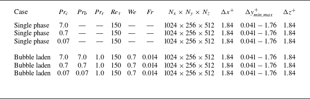


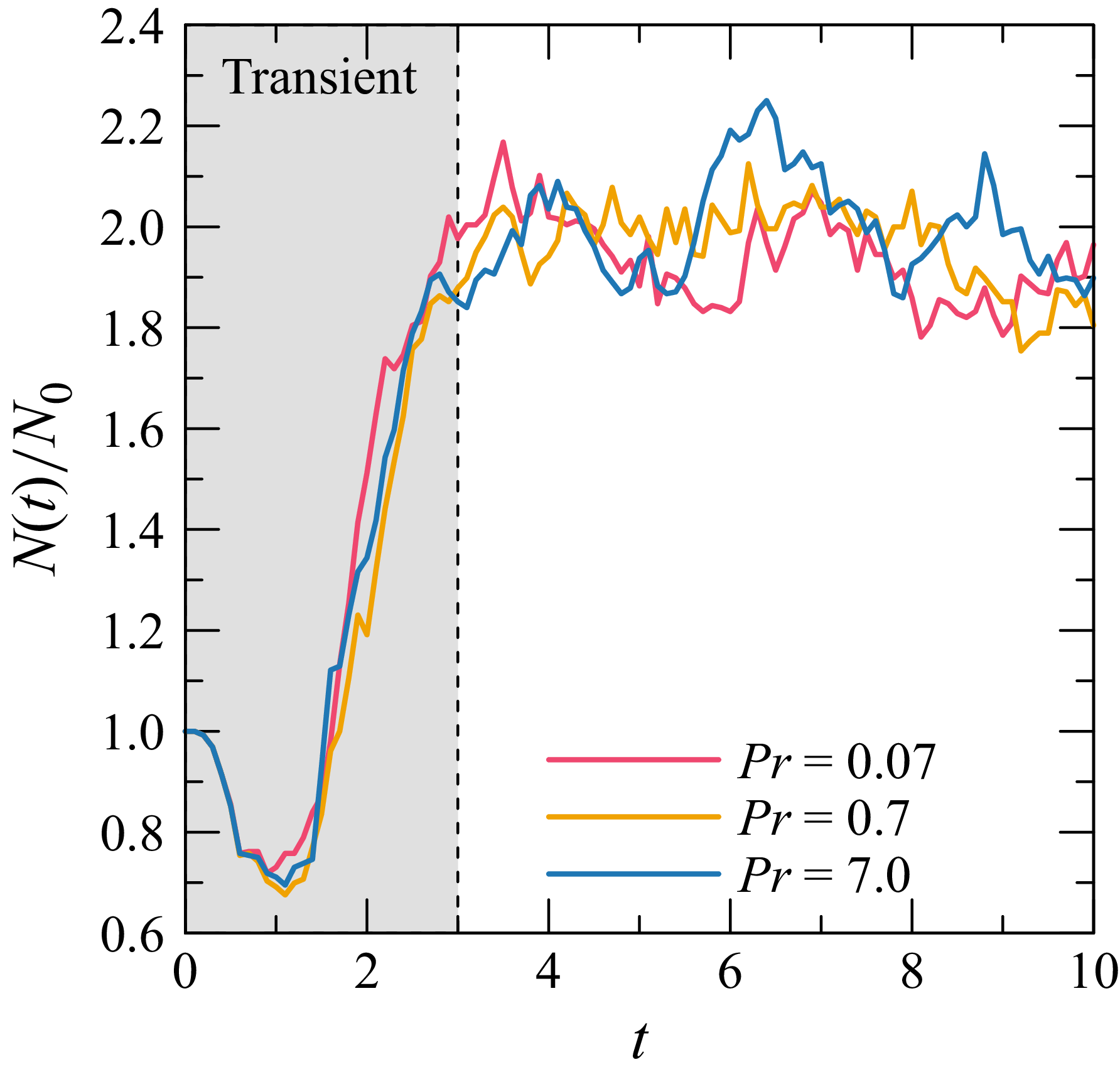


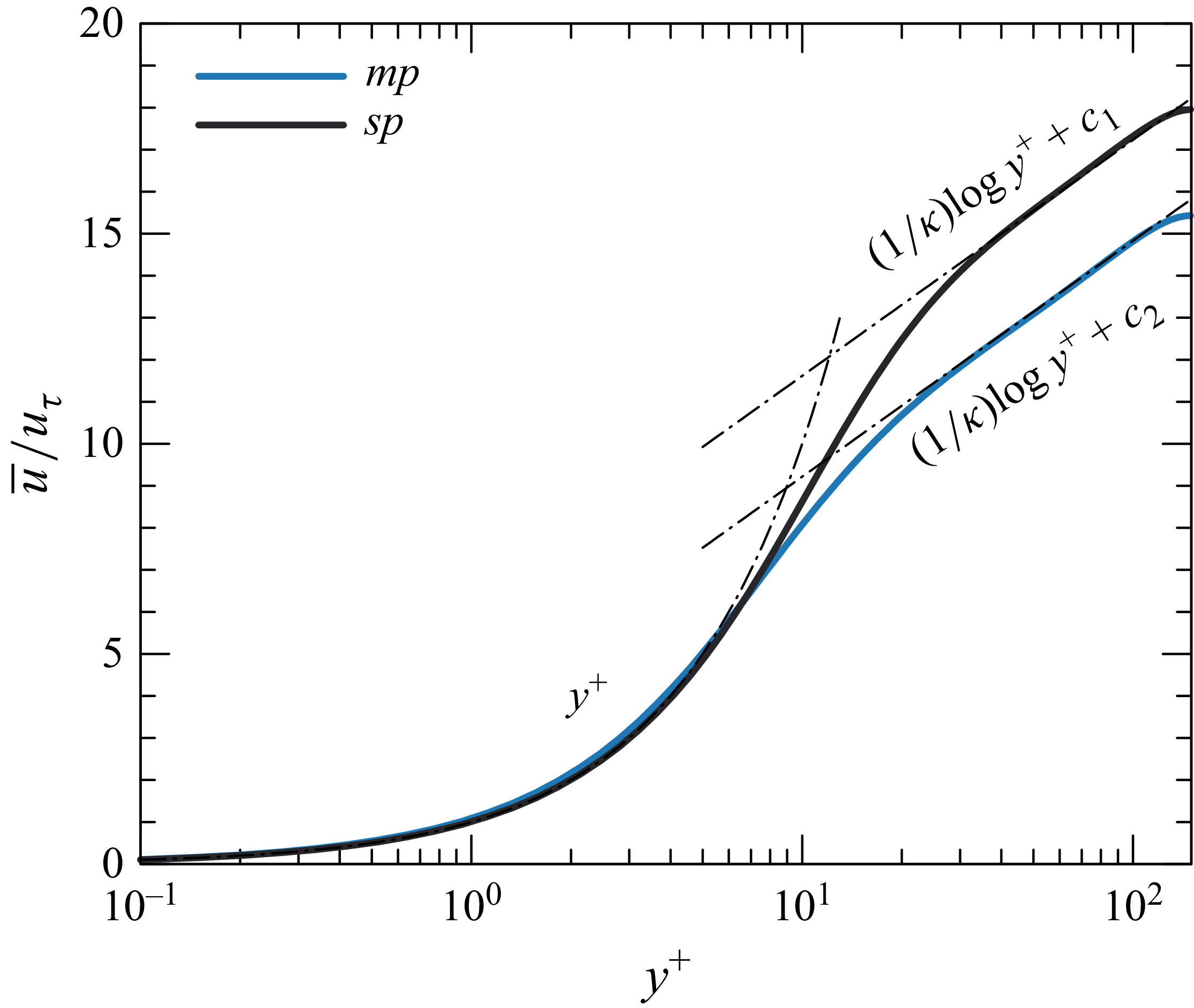


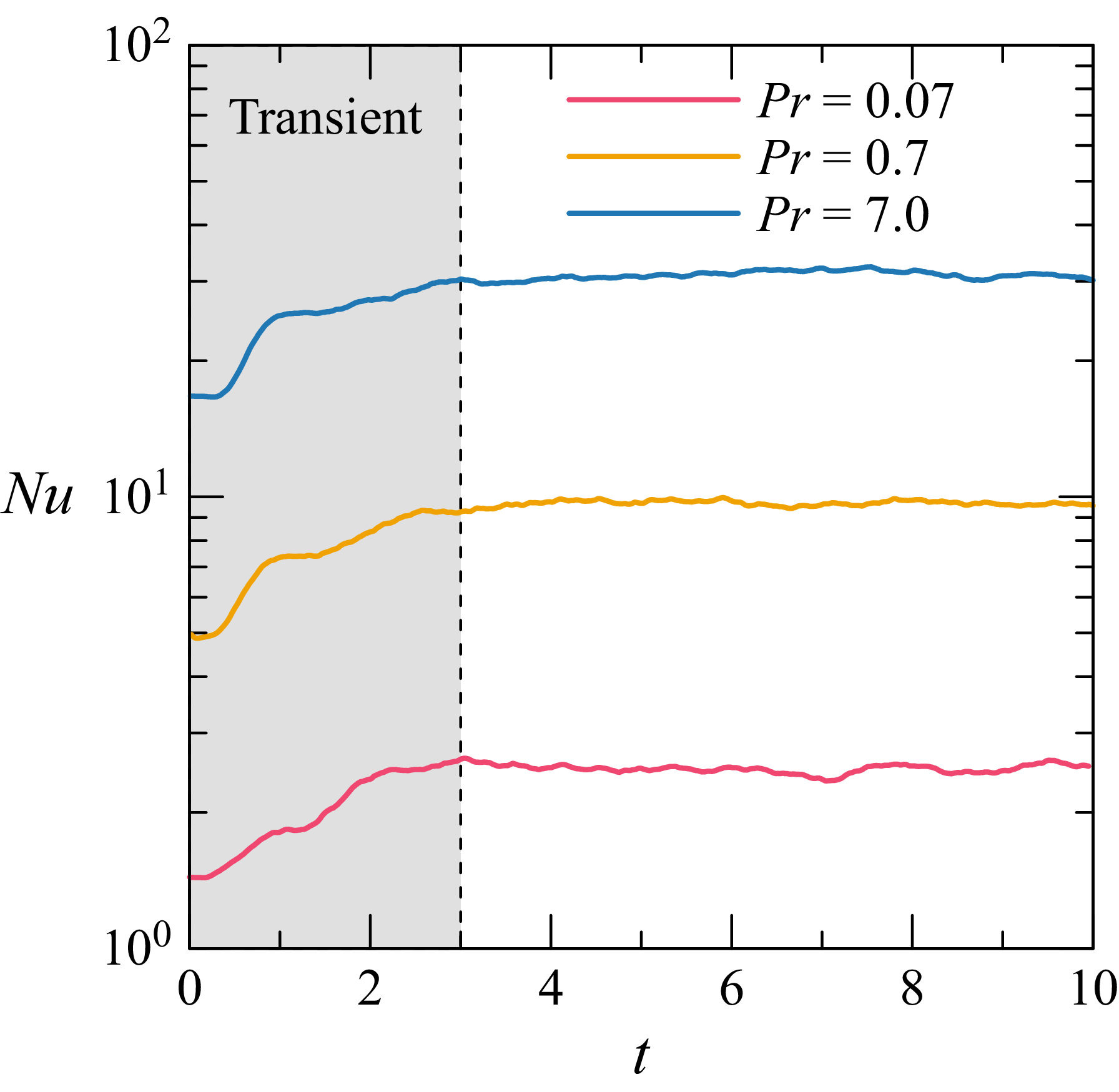


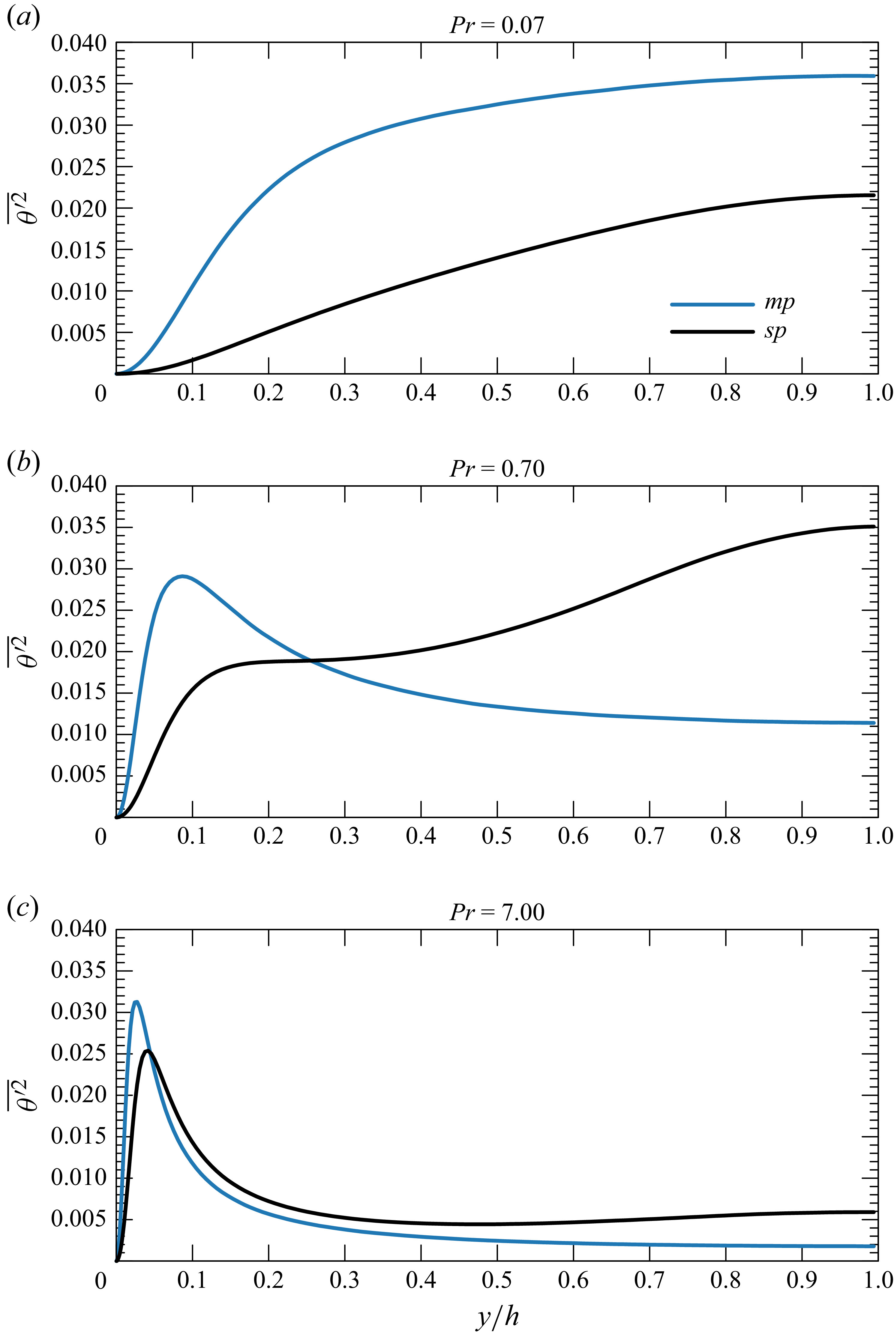


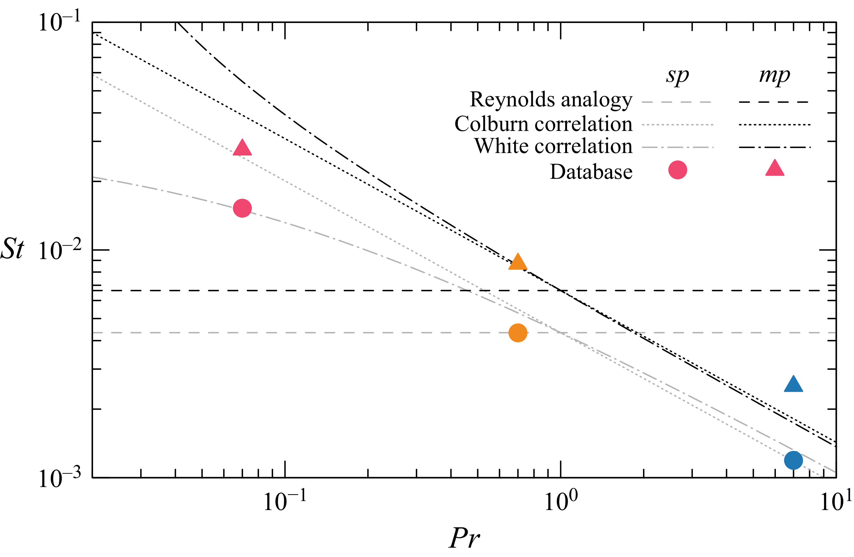


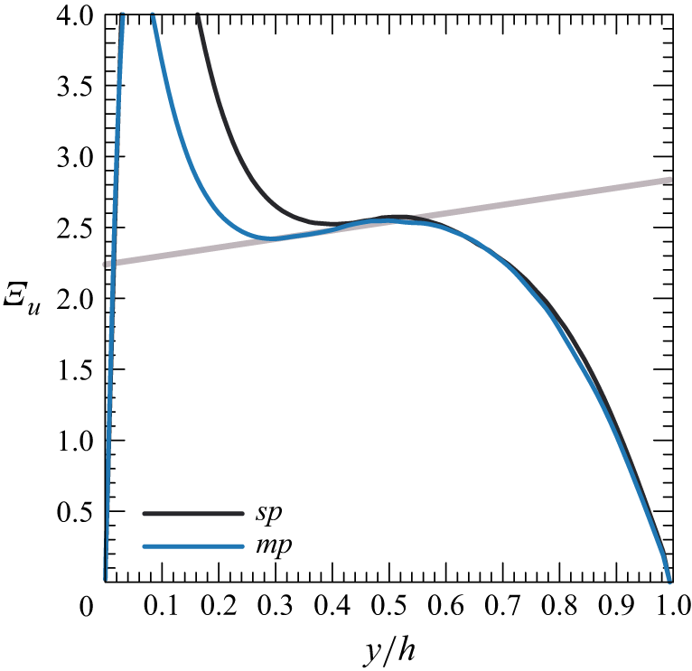
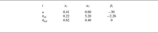


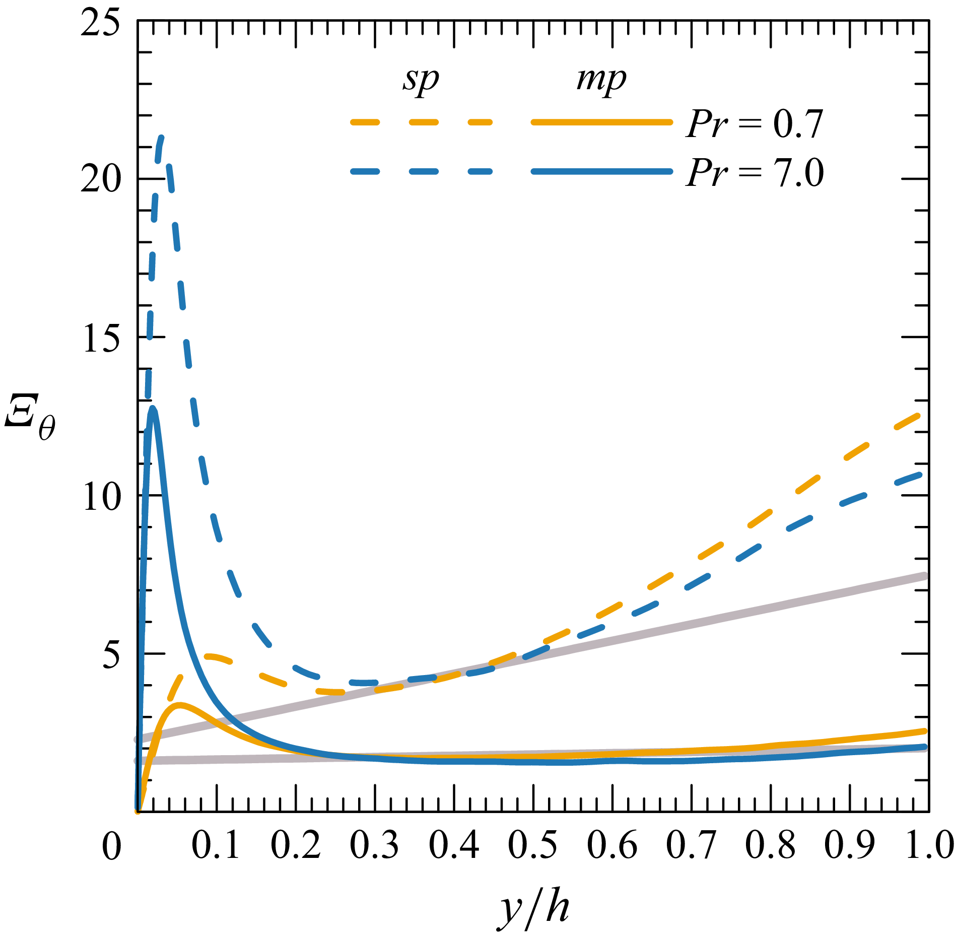

 Open access