2. Assumptions and main results

2.1. Assumptions

Firstly, we make some basic assumptions.

$(A1)$ As $n\to \infty,~b_n\to0$ and $nb_n/ \log n \to \infty$;

$(A2)$ $\{X_i, i \geq 1\}$ is a sequence of stationary $\alpha$-mixing random variables. $X_1$ has an uniformly continuous density $f(x)$ on the real line $\mathbb{R}$ and the mixing coefficient satisfies $\alpha(n)=O(n^{-\lambda})$ for some $\lambda \geq 2$;

$(A3)$ The joint density function $f_{ij}(x, y)$ of $(X_i, X_j)$ exists and for some positive constant $M$, it satisfies

\begin{eqnarray*} \sup\limits_{(x,y)\in \mathbb{R}^2}|f_{ij}(x, y)-f(x)f(y)| \leq M,~\textrm{for any~} i\neq j ; \end{eqnarray*}

$(A4)$ The density function $f(x)$ satisfies the Lipschitz condition of order $1$, i.e., for all $x, y \in \mathbb{R}$ and some $L \gt 0$,

\begin{eqnarray*}|f(x)-f(y)| \leq L|x-y|;\end{eqnarray*}

$(A5)$ $E|X_1|^{1/T} \lt \infty$ for some $T \gt 0$.

Remark 2.1. The assumptions are general and also weaker than those assumed in the literature, such as [Reference Yang12], [Reference Huang and Xing5], [Reference Kang, Abbasi, Wang, Xu, Wang and Tang6] and [Reference Younso13]. $(A1)$ ensures asymptotic unbiasedness and adequate bin occupancy for variance control; $(A2)$ facilitates Bernstein-type inequalities for dependent data; $(A3)$ restricts joint densities, which is milder than uniform boundedness often required in kernel estimation; $(A4)$ is a standard Lipschitz condition; $(A5)$ requires a weaker moment condition, which is essential for modeling heavier-tailed data, which significantly expands applicability to real-world datasets where higher moments may not exist. This contrasts with the stronger order- $2/T$ moment required for strong consistency in [Reference Yang12], for instance.

Next, we give the main results as follows.

2.2. Main results

Theorem 2.2. Suppose that $(A1)--(A4)$ are satisfied. If

(2.1)\begin{equation} g(n, 1) := b_n^{-1} (nb_n/ \log n)^{-\lambda} \to 0, \end{equation}

then for any $x\in \mathbb{R}$,

(2.2)\begin{equation} \left|f_{n} (x)- f(x)\right|= o(1) \textrm{~in~ probability}. \end{equation}

Consider the optimal binwidth $b_n = Cn^{-1/5}$ (Carbon et al. (1979)), it is clear that $(A1)$ is satisfied. Hence, we get the following corollary.

Corollary 2.3. Suppose that $b_n = Cn^{-1/5}$ and $(A2)--(A3)$ are satisfied. Then for any $x\in \mathbb{R}$, (2.2) holds.

Theorem 2.4 Suppose that $(A1)--(A5)$ are satisfied. Then we have the following two statements:

(1) If

(2.3)\begin{equation} g(n, 2) := b_n^{-2} (nb_n/ \log n)^{-\lambda} \to 0, \end{equation}

then for any compact subset $D$ of $\mathbb{R}$,

(2.4)\begin{equation} \sup\limits_{x\in D} \left|f_{n} (x)- f(x)\right|= o(1) \textrm{~in~ probability}; \end{equation}

(2) If $g(n, 2)n^T\to 0,$ then

(2.5)\begin{equation} \sup\limits_{x\in \mathbb{R}} \left|f_{n} (x)- f(x)\right|=o(1) \textrm{~in~ probability}. \end{equation}

Analogously, we have the following corollary.

Corollary 2.5. Suppose that $b_n = Cn^{-1/5}$ and $(A2)--(A5)$ are satisfied. Then for any compact subset $D$ of $\mathbb{R}$, (2.4) holds. Furthermore, if $\lambda \gt \max\left\{2, \frac{2+5T}{4} \right\}$, then (2.5) holds.

Remark 2.6. The following theorem is the rate of the uniformly weak consistency for frequency polygon estimation of the density function under $\alpha$-mixing samples.

Theorem 2.7. Suppose that $(A1)--(A5)$ are satisfied. Denote $R_n=\max\left\{b_n ,\left(\frac{\log n}{n b_n}\right)^{1/2}\right\}$. Then we have the following two statements:

(1) If

(2.6)\begin{equation} g(n, 3) := b_n^{-2} (nb_n/ \log n)^{-\lambda/2+1/2} \to 0, \end{equation}

then for any compact subset $D$ of $\mathbb{R}$,

(2.7)\begin{equation} \sup\limits_{x\in D}\left| f_{n} (x)-f(x)\right|= O\left(R_n\right) {~in~ probability}; \end{equation}

(2) If $g(n, 3)n^T\to 0,$ then

(2.8)\begin{equation} \sup\limits_{x\in \mathbb{R} }\left| f_{n} (x)-f(x)\right|= O\left(R_n\right) {~in~ probability}. \end{equation}

Clearly, we have $R_n\to 0$ as $n\to \infty$, so Theorem 2.7 implies that $f_n(x)$ converges in probability to $f (x)$ with the rate $R_n$. Analogously, we have the following corollary.

Corollary 2.8. Suppose that $b_n = Cn^{-1/5}$ and $(A2)--(A5)$ are satisfied. If $\lambda \gt 2$, then for any compact subset $D$ of $\mathbb{R}$, (2.7) holds. Furthermore, if 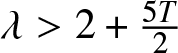$\lambda \gt 2+\frac{5T}{2} $, then (2.8) holds.

Remark 2.9. From Corollary 2.3, if the binwidth $b_n = Cn^{-1/5}$, then 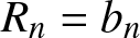$R_n=b_n$; if the binwidth 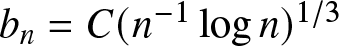$b_n = C(n^{-1} \log n)^{1/3}$, then 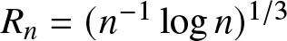$R_n=(n^{-1} \log n)^{1/3}$, which is the optimal rate of convergence for the histogram density estimation in the i.i.d. case.

Remark 2.10. Theorems 2.4 and 2.7 state the uniformly weak consistency for frequency polygon estimation of density function. Compared with the corresponding results of [Reference Yang12] or other related literatures establishing strong consistency under the moment condition $E|X|^{2/T} \lt \infty$ for some $T \gt 0$, it is noted that a lower moment condition is assumed here, which is $E|X|^{1/T} \lt \infty$ for some $T \gt 0$.

Remark 2.11. In fact, the weaker the requirements for convergence, the easier it is for a sequence of random variables to have a limit, we know that the existence of weak consistency can solve some issues. It is an important subject to obtain weak convergence results under weak conditions, and our results generalize and improve the existing ones in the literature.

3. Simulation study

This simulation study aims to verify the theoretical consistency of the frequency polygon estimator under finite $\alpha$-mixing samples and to examine its performance across different dependence strengths.

We generate data from an ARMA(1,1) model, a standard framework for studying dependent processes. Consider the ARMA(1,1) model:

(3.1)\begin{equation} X_t = \phi X_{t-1} + \varepsilon_t-\theta \varepsilon_{t-1}, \end{equation}

where $\{\varepsilon_t, t \geq 1\}$ are independent and identically distributed, $\varepsilon_i \sim N(0, \sigma_\varepsilon^2)$, $| \phi| \lt 1, |\theta| \lt 1$ and $\sigma_\varepsilon^2= (1-\phi^2)/(1-2 \phi \theta + \theta^2)$. Obviously, we know $X_t \sim N(0,1)$. We know from [Reference Fan and Yao4] and Yang (2023) that $\{X_t, t \geq 1\}$ is an $\alpha$-mixing and stationary time series with $\alpha(k) = O(|\phi|^k)$ for the case $\phi\neq\theta$.

The specific scenarios are defined by the autoregressive parameter $\phi$, which directly controls the dependence strength. We consider $\phi\in \{0,0.1,0.3,0.4,0.5,0.6,0.8\}$, covering a spectrum from independence ( $\phi=0$) to strong positive dependence ( $\phi=0.8$). For each $\phi$, complementary moving-average parameters $\theta$ are selected to form distinct. Sample sizes are set to $n = 1250,$ $2500$, $5000$, and $10^4$ to assess the estimator’s behavior as the sample increases.

[Reference Carbon, Garel and Tran3] proved the best possible choice of the binwidth, namely $h_{FP} =2\left(\frac{15}{49nR^{''}(f)} \right)^{1/5}$, and $R^{''}(f)=\frac{3}{8\sqrt{\pi}\sigma^5}$ can be calculated in our experiments, then optimal binwidth in our experiments is $b_{n}=h_{FP}= 2.153366 n^{-1/5}\sigma$. It is called the optimal binwidth under the integrated mean squared error. The experiment is repeated $N=100$ times in each scenario. For $x_i =-3 + 0.05(i -1)$ where $1 \leq i \leq m$ and 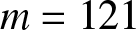$m = 121$, we compute the estimates $f_n(x_i)$, the global mean absolute relative deviations

(3.2)\begin{equation} GMARD_f(n) = \frac{1}{Nm}\sum_{i=1}^{m}\sum_{k=1}^{N}\frac{| f_n(x_i,k)-f (x_i)|}{f (x_i ) }, \end{equation}

and the values of

(3.3)\begin{equation} GR_f(n):= \frac{1}{Nm}\sum_{i=1}^{m}\sum_{k=1}^{N}\frac{| f_n(x_i,k)-f (x_i )|}{R_n}, \end{equation}

where $f (x )$ is the density function of standard normal distribution, 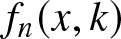$f_n(x, k)$ is the estimate of density function in $k$-th experiment and $R_n$ takes $b_n$ here. $GMARD_f(n)$ measures the absolute estimation error 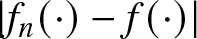$\left|f_n (\cdot)-f (\cdot)\right|$, while $GR_f(n)$ quantifies the relative rate at which this error shrinks in comparison to the theoretical convergence rate $R_n$. 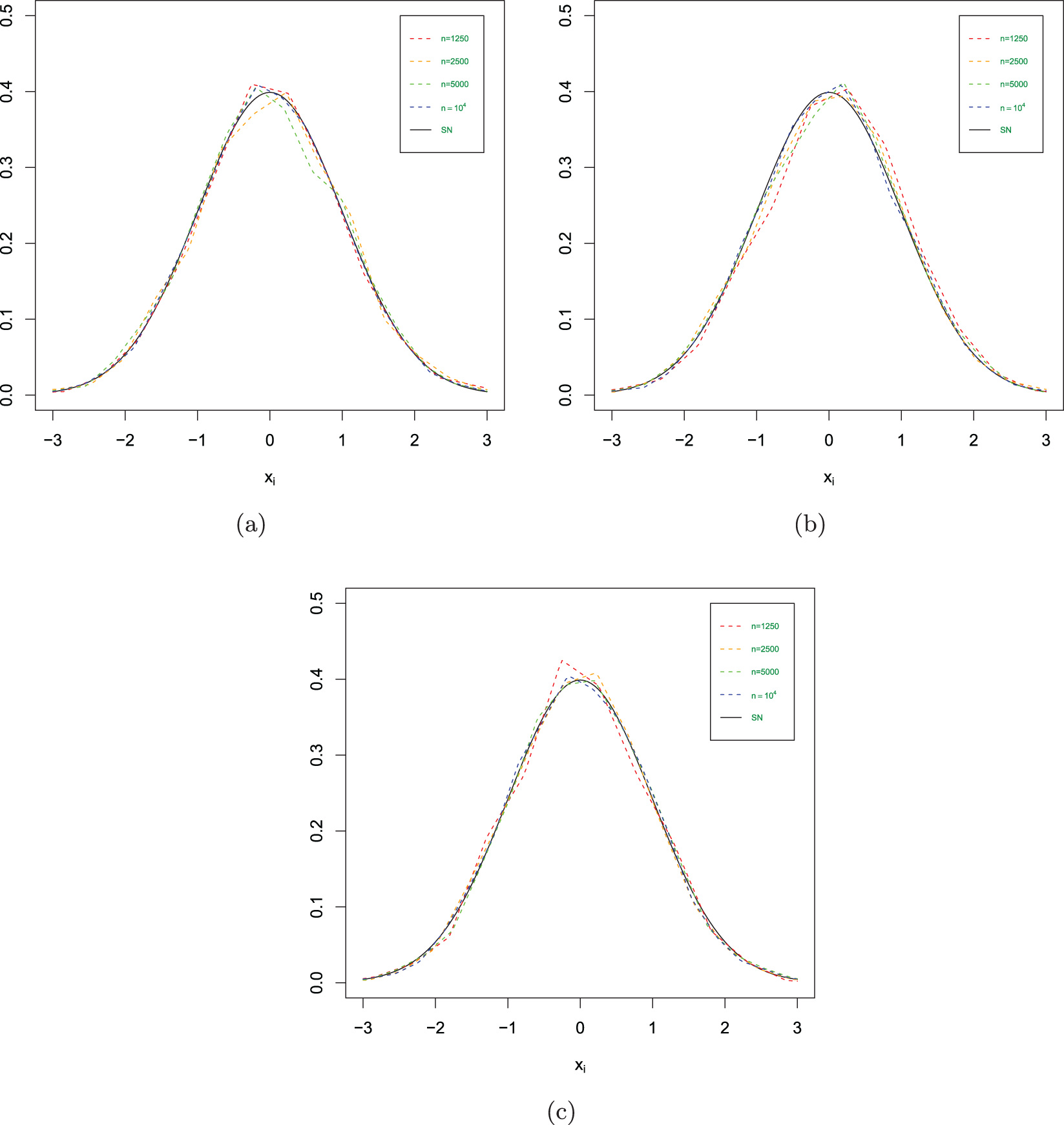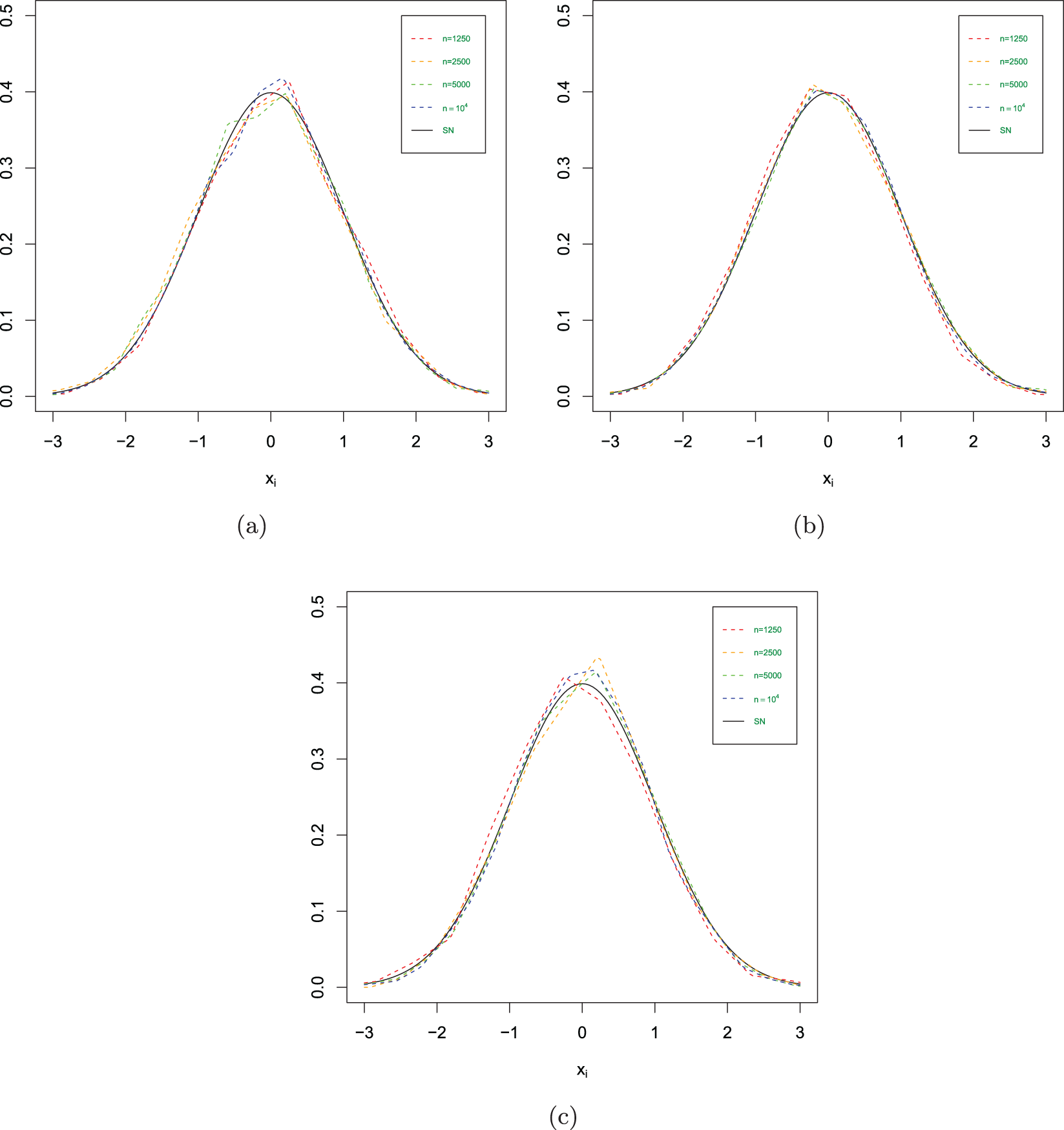Specifically, the estimates $f_n(x )$ in different scenarios are shown in Figs. 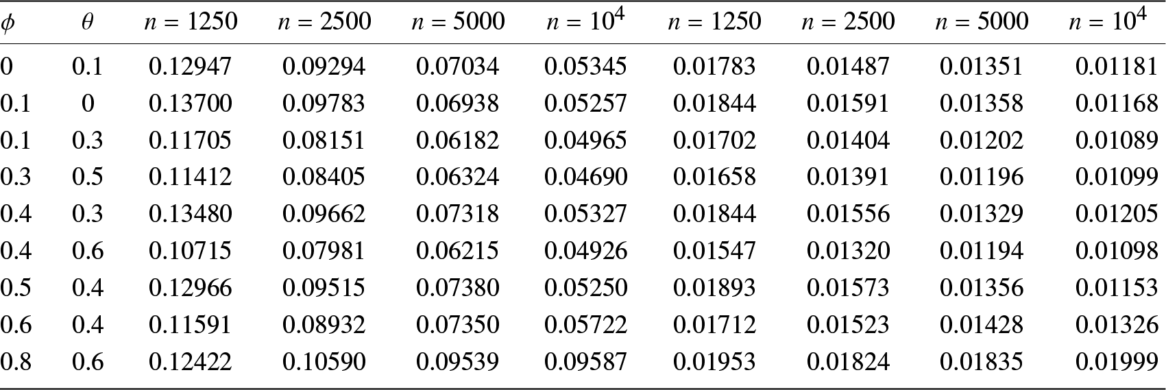1–3, the $GMARD_f(n)$ and $GR_f(n)$ obtained in different scenarios are listed in Tab. 1.

Figure 1.

The estimated values in different scenarios. (a) $\phi= 0$ and $\theta=0.1$. (b) 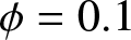$\phi= 0.1$ and $\theta=0$. (c) $\phi= 0.1$ and 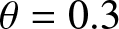$\theta=0.3$.

Figure 2.

The estimated values in different scenarios. (a) 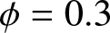$\phi= 0.3$ and 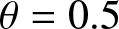$\theta=0.5$. (b) 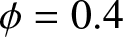$\phi= 0.4$ and $\theta=0.3$. (c) $\phi= 0.4$ and $\theta=0.6$.

Figure 3.

The estimated values in different scenarios. (a) 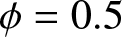$\phi= 0.5$ and 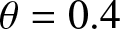$\theta=0.4$. (b) 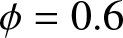$\phi= 0.6$ and $\theta=0.4$. (c) 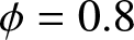$\phi= 0.8$ and $\theta=0.6$.

Table 1.

The values of $GMARD_f(n)$ (left) and $GR_f(n)$ (right) in different scenarios.

Concluding remarks

(1) Figs. 1–3 show us that when the sample size increases, the fitting effects of the three curves become better based on the same sample dependence. While the dependence enhances, the fitting effects of these three curves also become worse under the same sample size. Furthermore, as sample sizes increase, the estimation quality also correspondingly improves.

(2) Tab. 1 reveals that higher values of $ \phi $ (e.g., $\phi = 0.8 $) introduce stronger dependence and long-range dependence in the series, leading to increased estimation errors (e.g., $GMARD_f(n$) up to 0.09587 for $n = 10^4$).

(3) Increasing $\theta$ (e.g., $\theta = 0.6$ for $\phi = 0.4$) can counteract the dependence induced by $\phi$ to some extent, and then reduce estimation errors (e.g., $GMARD_f(n)$ decreases from 0.13480 to 0.10715 for $n = 1250$).

(4) Weak dependence (e.g., $\phi = 0.1$ or balanced $\phi/\theta$ pairs like $\phi = 0.3, \theta = 0.5$) yields the better performance of estimation, with lower $GMARD_f(n)$ and $GR_f(n)$ values across sample sizes.

(5) With the increasing of the sample size, the value of $GR_f(n)$ decreases. Mathematically, $GR_f(n)$ is a representation for the convergence rate of the estimation $f_n(\cdot)$, indicating that $f_n(\cdot)$ either maintains the same convergence rate as $R_n$ or even surpasses it.

In short, $GMARD_f(n)$ decrease with the increase of sample size $n$, which shows that the estimation is consistent based on $\alpha$-mixing samples in this case. Strong dependence reduces estimation quality, and at this time, larger samples are needed as compensation. These findings demonstrate our theoretical results.

4. Real data analysis

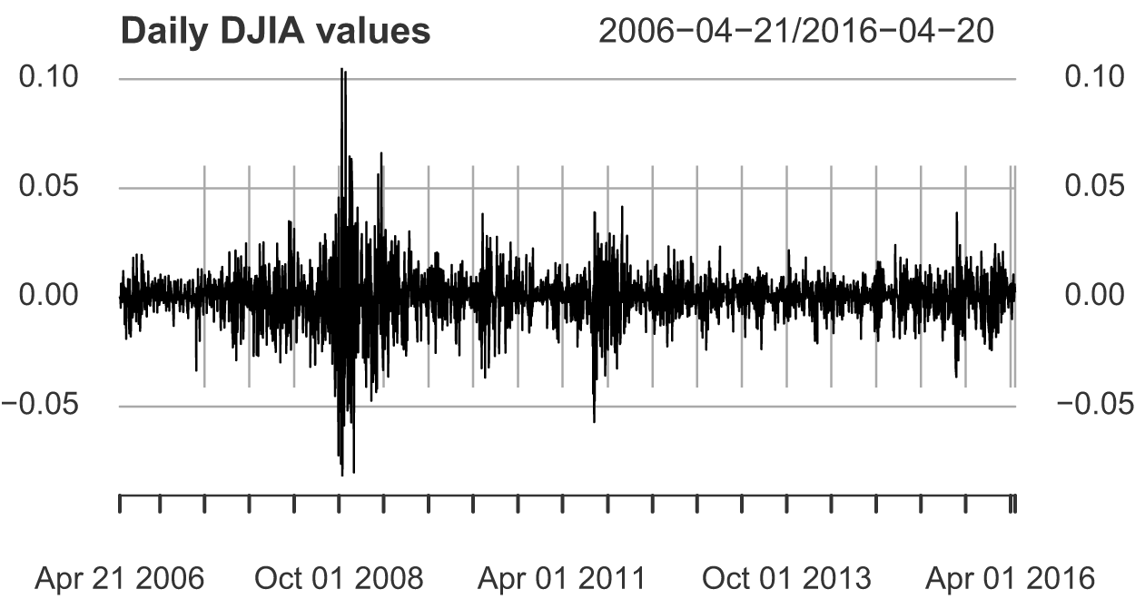
The statistical analysis of continuous data is a surprisingly recent development. The goal of this section is to demonstrate the practical applicability of the frequency polygon estimator for financial return data, which exhibits volatility clustering and heavy tails. As an example of financial time series data, Fig. 4 shows the rate of the daily return (or percentage change) of Dow Jones Industrial Average (DJIA) from April 21st, 2006 to April 20th, 2016. This is the typical rate of return data. The average value of the series seems to be stable, and the average rate of return is close to zero. However, the periods with great fluctuations (changes) tend to gather together. One problem in the analysis of these types of financial data is to estimate the density function, which is helpful to predict the volatility of future returns. Let $d_t$ be the actual value of DJIA, $r_t=(d_t-d_{t-1})/d_{t-1}$ is the rate of return, then we have $1+r_t=d_t/d_{t-1}$, and $\log(1+r_t)=\log(d_t/d_{t-1})=\log(d_t)-\log(d_{t-1})\approx r_t$. This data set can also be obtained in the R package (astsa).

Figure 4.

The rate of the daily return (or percentage change) of DJIA from April 20th, 2006 to April 20th, 2016.

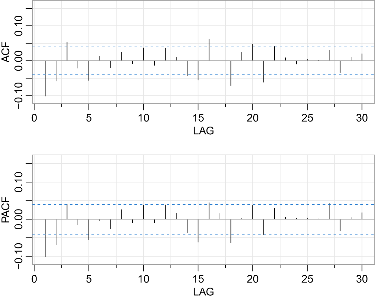
Observing Fig. 4, we note that the mean remains nearly constant, oscillating around 0, indicating that the series might be stationary. The PACF’s significant spike at lag 2 (exceeding the confidence band) necessitates AR(2), while the ACF’s gradual decay implies MA terms are needed. Fig. 5 suggests that the dataset could be an ARMA(2,2) process. After conducting the augmented Dickey-Fuller (ADF) unit root test, we find that the test statistic is $-39.8484$, which is less than the critical value of $-2.58$ at the 1% significance level 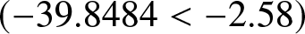$(-39.8484 \lt -2.58)$. Therefore, at the 1% significance level, we reject the null hypothesis, concluding that the series is stationary. A stationary ARMA process $\{X_t,t\geq1\}$ is $\alpha$-mixing according to [Reference Fan and Yao4].

Figure 5.

The ACF and PACF plots of the daily return rate of DJIA from April 20th, 2006 to April 20th, 2016.

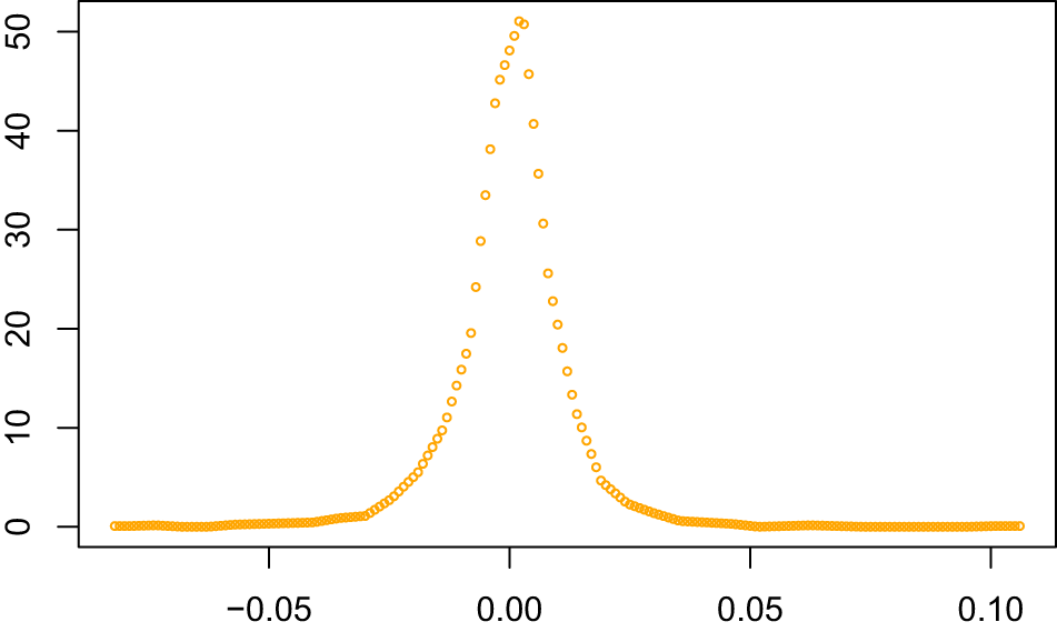
By employing the calculation method in the Simulation study section, we can derive the frequency polygon estimation of the daily return rate (or percentage change rate) of DJIA. Figure 6 shows leptokurtic features (peaked center and fat tails) compared to the red normal distribution curve, consistent with empirical finance data.

Figure 6.

The estimated density function of daily return rate of DJIA.

In addition, the GARCH (generalized autoregressive conditional heteroskedasticity) model is particularly adept at capturing the variability of volatility in financial time series, and it can provide valuable insights for risk management and investment strategies. The frequency polygon estimator provides a complementary nonparametric approach for modeling return distributions. To delve deeper into comprehending the volatility pattern and structure specifically exhibited by the daily return rate of DJIA, we utilize the “rugarch” package in R to analyze the data set, and then derive the conditional variance equation of GARCH(1,1) model as follows:

\begin{equation*}h_t = 2.192579\times10^{-6} + 0.1209623 \varepsilon_{t-1}^2 + 0.8616528 h_{t-1}.\end{equation*}

It can be noted that the aggregate value of 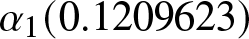$\alpha_1 (0.1209623)$ and 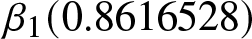$\beta_1 (0.8616528)$ approaches unity, which strikingly emphasizes the tenacity of volatility and the significant clustering effect within the financial time series. This observation highlights the persistent nature of market turbulence, where periods of high volatility tend to be succeeded by further volatility. The data captures the essence of volatility clustering in financial data.

5. Lemmas

Firstly, we make some notations.

Denote $a_{n,j;1} =\frac{1}{2}+j-\frac{x}{b_n},~a_{n,j;2} =\frac{1}{2}-j+\frac{x}{b_n}$ and $U_{n,j} = [(j-1/2)b_n, (j+1/2)b_n), j=0,\pm1,\pm2,\cdots$. Then the frequency polygon estimator (1.2) may be rewritten as

(5.1)\begin{equation} f_n (x) = a_{n,j;1}f_{n,j} + a_{n,j;2} f_{n,j+1}\textrm{~for~} x \in U_{n,j}. \end{equation}

Furthermore, let

(5.2)\begin{equation} Y_{n,j;i} = I((j-1)b_n \leq X_i \lt jb_n), Z_{n,j;i} = Y_{n,j;i} - EY_{n,j;i},~ i\geq 1. \end{equation}

Then we have 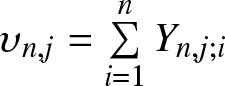$\upsilon_{n,j} =\sum\limits_{i=1}^n Y_{n,j;i}$ and

(5.3)\begin{equation} f_n (x) = a_{n,j;1}\frac{\sum\limits_{i=1}^n Y_{n,j;i}}{nb_n}+ a_{n,j;2}\frac{\sum\limits_{i=1}^n Y_{n,j+1;i}}{nb_n}. \end{equation}

It is clear that the weights $a_{n,j;1}$ and $a_{n,j;2}$ satisfy

(5.4)\begin{equation} 0 \lt a_{n,j;1}, a_{n,j;2} \lt 1 \textrm{~and~} a_{n,j;1} + a_{n,j;2}= 1. \end{equation}

Denote $p_{nj}:=EY_{n,j;i}=P((j-1)b_n \leq X_i \lt jb_n)$. It is also clear that 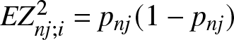$EZ_{nj;i}^2=p_{nj}(1-p_{nj})$.

This section provides several important lemmas, which play vital roles and will be used in the subsequent proofs of the main results. The first one is the moment inequality on estimating the upper bound of $2$-nd moment for the partial sums of random variables.

Lemma 5.1. (cf. Yang, 2017, Lemma 3.3)

Suppose that 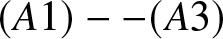$(A1)--(A3)$ hold, and the integers $a$ and $m$ satisfy $0\leq a \lt a+m\leq n$. Then there exists a positive constant $C$, which does not depend on $n,j, a$ and $m$, such that

\begin{equation*}E\left(\sum_{i=a+1}^{a+m}Z_{nj;i} \right)^2 \leq Cmb_n.\end{equation*}

The following one is the probability inequality for $\alpha$-mixing random variables, which is an important tool in the later proofs.

Lemma 5.2. (cf. Wei et al., [Reference Wei, Yang, Yu, Yang and Xing9], Lemma 3.3)

Let $\{\xi_i, i \geq 1\}$ be a sequence of real-valued $\alpha$-mixing random variables with $E\xi_i = 0$ and $ |\xi_i|\leq b \lt \infty~a.s.$, $\{k_n, n \geq 1\}$ be positive integers such that $1\leq k_n \leq n/2$. Then for any $\epsilon \gt 0$,

\begin{eqnarray*} P\left(\left|\sum\limits_{i=1}^{n} \xi_i\right| \gt n\epsilon \right) \leq 4 \exp \left( -\frac{n\epsilon^2}{12(3\sigma_n^2+bk_n\epsilon)} \right) +36b\epsilon^{-1}\alpha(k_n), \end{eqnarray*}

where $\sigma_n^2=n^{-1}\sum_{j=1}^{2m_n+1}EV_j^2$, $m_n=\lfloor n/(2k_n)\rfloor$, $V_j=\sum_{(j-1)k_n \lt i \leq jk_n}\xi_i~ (j=1,2,\cdots,2m_n)$ and $V_{2m_n+1}=\sum_{i =2m_nk_n+1}^n\xi_i$.

In order to clarify the proofs of the main results, we provide the following two lemmas. The first one is inspired by [Reference Yang12].

Lemma 5.3. If $f(x)$ is uniformly continuous in $\mathbb{R}$, then

(5.5)\begin{equation} \sup_{x\in \mathbb{R}}\left|Ef_n(x)-f(x)\right|=o(1). \end{equation}

If $f(x)$ satisfies the Lipschitz condition of order $1$, i.e., the condition $(A4)$, then

(5.6)\begin{equation} \sup_{x\in \mathbb{R}}\left|Ef_n(x)-f(x)\right|=O(b_n ). \end{equation}

Proof. It is easy to see that

\begin{eqnarray*} \sup_{x\in \mathbb{R}}\left|Ef_n(x)-f(x)\right|=\sup_{-\infty \lt j \lt \infty}\sup_{x\in U_{nj}}\left|Ef_n(x)-f(x)\right|. \end{eqnarray*}

Note that for $ x\in U_{nj}$,

\begin{equation*}\left|Ef_n(x)-f(x)\right|\leq \frac{1}{b_n}\int_{(j-1)b_n}^{jb_n}\left| f (y)-f(x)\right|dy\textrm{~and~}b_n\to 0.\end{equation*}

If $f (x)$ is uniformly continuous in $\mathbb{R}$, then for $\epsilon \gt 0$, as $n$ sufficiently large,

\begin{equation*} \int_{(j-1)b_n}^{jb_n}\left| f (y)-f(x)\right|dy\leq \epsilon b_n.\end{equation*}

Hence, the desired result (5.5) is derived.

If $f(x)$ satisfies the condition $(A4)$, then as $n$ sufficiently large, we have

\begin{equation*} \int_{(j-1)b_n}^{jb_n}\left| f (y)-f(x)\right|dy\leq C b_n^2.\end{equation*}

Hence, the desired result (5.6) is derived.

Lemma 5.4. Suppose that there exists some $T \gt 0$ such that $E|X|^{1/T} \lt \infty$. Denote $T_n=(-\infty,-n^T)\bigcup(n^T,\infty)$ and 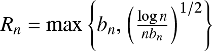$R_n=\max\left\{b_n,\left(\frac{\log n}{n b_n}\right)^{1/2}\right\}$. Then we have

(5.7)\begin{equation} \sup_{x\in T_n} f_n(x)=O_P\left( R_n\right). \end{equation}

Furthermore, suppose that the density function $f(x)$ is continuous. Then we have

(5.8)\begin{equation} \sup_{x\in T_n} f (x)=O\left( n^{-(1+T)}\right). \end{equation}

Proof. In fact, if we want to get (5.7), we only need to prove that for every $\epsilon \gt 0$, there exist $M_\epsilon$ and $N_\epsilon$ such that for all $n \gt N_\epsilon$

(5.9)\begin{equation} P\left(\frac{\sup_{x\in T_n} f_n(x)}{R_n} \gt M_\epsilon \right) \lt \epsilon. \end{equation}

Note that

(5.10)\begin{equation} \sum_{k=1}^\infty kP\left(k^T \lt |X|\leq (k+1)^T\right) \leq CE|X|^{1/T} \lt \infty. \end{equation}

We can obtain by (5.10) that for sufficiently large $n$

(5.11)\begin{eqnarray}P\left(\frac{\sup_{x\in T_n} f_n(x)}{R_n} \gt M_\epsilon \right)&\leq & P\left( \sup_{x\in T_n} f_n(x) \gt 0\right)\nonumber\\ &\leq& nP\left(X\in T_n\right)=nP\left(|X| \gt n^T\right)\nonumber\\ &=&\sum_{k=n}^\infty nP\left(k^T \lt |X|\leq (k+1)^T\right)\nonumber\\ &\leq&\sum_{k=n}^\infty kP\left(k^T \lt |X|\leq (k+1)^T\right) \lt \epsilon.\end{eqnarray}

Since 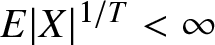$E|X|^{1/T} \lt \infty$ and the density function $f (x)$ is continuous, we obtain $f (x) = o\left(|x|^{-(1/T+1)}\right)$ as $|x|\to \infty$. Therefore, for sufficiently large $n$, we have

(5.12)\begin{eqnarray}\sup_{x\in T_n}f (x)&=&\sup_{|x| \gt n^T}f (x) \leq \sup_{|x| \gt n^T} \left(\frac{|x|}{n^T} \right)^{1/T+1} f (x) \nonumber\\ &=& n^{-(1+T)} \sup_{|x| \gt n^T} |x|^{1/T+1} f (x) \leq Cn^{-(1+T)}.\end{eqnarray}

Hence, the proof of Lemma 5.4 is completed.

6. Proofs of main results

6.1. Proof of Theorem 2.2

Recall that the partition $\cdots \lt x_{-2} \lt x_{-1} \lt x_0 \lt x_1 \lt x_2\cdots$ of the real line $\mathbb{R}$ and equal intervals $I_{n,j} :=[(j-1)b_n, jb_n)$ of length $b_n$, where $b_n$ is the binwidth and $j = 0, \pm1, \pm2, \cdots$, $U_{nj}=\left[(j-1/2)b_n, (j+1/2)b_n\right)$. From Lemma 5.3, we only need to prove that for each $j$ and any $x\in U_{nj}$,

(6.1)\begin{equation} \left|f_n(x)- Ef_n(x)\right|=o(1) \textrm{~in~ probability.} \end{equation}

Noting that $EZ_{nj;i}=0$ and $|Z_{nj;i}|\leq 1$, we get by Lemma 5.1 that

\begin{eqnarray*} E V_j^2=E\left( \sum\limits_{(j-1) k_n \lt i \leq j k_n}Z_{nj;i} \right)^2 \leq Ck_nb_n, \end{eqnarray*}

and thus

\begin{eqnarray*} \sigma_n^2=n^{-1}\sum_{j=1}^{2m_n+1}EV_j^2\leq Cn^{-1}k_n (2m_n+1)b_n\leq Cb_n. \end{eqnarray*}

Hence, we have that for any $\varepsilon \gt 0$ and $x\in U_{nj}$

(6.2)\begin{align}&P\left( \left|f_n(x)- Ef_n(x)\right| \gt \varepsilon\right)\nonumber\\ &= P\left( \left|a_{n,j;1}\sum\limits_{i=1}^{n}\left(Y_{n,j;i} -E Y_{n,j;i} \right)+a_{n,j;2}\sum\limits_{i=1}^{n}\left(Y_{n,j+1;i} -E Y_{n,j+1;i} \right) \right| \gt nb_n\varepsilon\right) \nonumber\\ &= P\left( \left|a_{n,j;1}\sum\limits_{i=1}^{n}Z_{n,j;i}+a_{n,j;2}\sum\limits_{i=1}^{n}Z_{n,j+1;i} \right| \gt nb_n\varepsilon\right) \nonumber\\ &\leq P\left( \left|\sum\limits_{i=1}^{n}Z_{n,j;i} \right| \gt \frac{nb_n\varepsilon}{2a_{n,j;1}}\right) +P\left( \left|\sum\limits_{i=1}^{n}Z_{n,j+1;i} \right| \gt \frac{nb_n\varepsilon}{2a_{n,j;2}}\right) .\end{align}

Note by Lemma 5.2 that

(6.3)\begin{align}P\left( \left|\sum\limits_{i=1}^{n}Z_{n,j;i} \right| \gt \frac{nb_n\varepsilon}{2a_{n,j;1}}\right)&\leq P\left( \left|\sum\limits_{i=1}^{n}Z_{n,j;i} \right| \gt \frac{nb_n\varepsilon}{2}\right)\nonumber\\ &\leq 4\exp\left\{ -\frac{nb_n^2 \varepsilon^2}{24(6\sigma_n^2+k_nb_n\varepsilon)}\right\}+72\varepsilon^{-1}b_n^{-1}\alpha(k_n) \nonumber\\ &\leq 4\exp\left\{ -\frac{nb_n \varepsilon^2}{24( C+k_n \varepsilon)}\right\}+72\varepsilon^{-1}b_n^{-1}\alpha(k_n) \nonumber\\ &\leq C\exp\left\{ -\frac{ \varepsilon^2}{24\left( \frac{C}{nb_n} +\frac{k_n}{nb_n} \varepsilon\right)}\right\}+C b_n^{-1} k_n^{-\lambda}.\end{align}

Taking $k_n=\frac{nb_n \varepsilon}{48\log n}$, we can get by (2.1) that the RHS of above inequality is less than

(6.4)\begin{align} C\exp\left\{ -\frac{\varepsilon^2 \log n}{24\left( \frac{\varepsilon^2}{48} +\frac{\varepsilon^2}{48}\right)}\right\}+C b_n^{-1} \left(\frac{nb_n }{\log n}\right)^{-\lambda} &\leq C\exp\left\{-\log n\right\}+C b_n^{-(1+\lambda)} n^{-\lambda} \left( \log n\right)^{\lambda}\nonumber\\ &\leq C n^{-1} +C b_n^{-(1+\lambda)} n^{-\lambda} \left( \log n\right)^{\lambda}\nonumber\\ &= C n^{-1} +C g(n, 1)=o(1). \end{align}

Similarly, we have

(6.5)\begin{equation} P\left( \left|\sum\limits_{i=1}^{n}Z_{n,j+1;i} \right| \gt \frac{nb_n\varepsilon}{2a_{n,j;2}}\right)=o(1), \end{equation}

which together with (6.2)–(6.4) yields (6.1).

Therefore, the proof of Theorem 2.2 is completed.

6.2. Proof of Theorem 2.4

Firstly, we prove (2.4). From Lemma 5.3, we only need to show that

(6.6)\begin{equation} \sup_{x\in D}\left|f_n(x)- Ef_n(x)\right|=o(1) \textrm{~in~ probability.} \end{equation}

Since $D$ is a compact subset of $\mathbb{R}$, we may denote $D=[-d, d]$ for some constant $d \gt 0$. Let 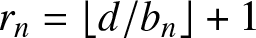$r_n=\lfloor d/b_n\rfloor+1$. Since $U_{nj}=\left[(j-1/2)b_n, (j+1/2)b_n\right)$, we have 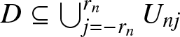$D\subseteq \bigcup_{j=-r_n}^{r_n}U_{nj}$.

Similar to the proof of Theorem 2.2, we obtain that 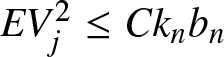$EV_j^2\leq Ck_nb_n $ and 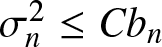$ \sigma_n^2 \leq C b_n$, and thus for any $\varepsilon \gt 0$,

(6.7)\begin{align}&P\left(\sup_{x\in D} \left|f_n(x)- Ef_n(x)\right| \gt \varepsilon\right)\nonumber\\ &\leq P\left(\max_{-r_n\leq j\leq r_n}\sup_{x\in U_{nj}} \left|f_n(x)- Ef_n(x)\right| \gt \varepsilon\right)\nonumber\\ &\leq \sum_{j= -r_n}^{r_n}P\left(\sup_{x\in U_{nj}} \left|f_n(x)- Ef_n(x)\right| \gt \varepsilon\right)\nonumber\\ &=\sum_{j= -r_n}^{r_n} P\left( \sup_{x\in U_{nj}} \left|a_{n,j;1}\sum\limits_{i=1}^{n}Z_{n,j;i}+a_{n,j;2}\sum\limits_{i=1}^{n}Z_{n,j+1;i} \right| \gt nb_n\varepsilon\right) \nonumber\\ &\leq\sum_{j= -r_n}^{r_n}P\left( \sup_{x\in U_{nj}} \left|\sum\limits_{i=1}^{n}Z_{n,j;i} \right| \gt \frac{nb_n\varepsilon}{2a_{n,j;1}}\right) +\sum_{j= -r_n}^{r_n}P\left( \sup_{x\in U_{nj}} \left|\sum\limits_{i=1}^{n}Z_{n,j+1;i} \right| \gt \frac{nb_n\varepsilon}{2a_{n,j;2}}\right)\nonumber\\ &\leq\sum_{j= -r_n}^{r_n}P\left( \left|\sum\limits_{i=1}^{n}Z_{n,j;i} \right| \gt \frac{nb_n\varepsilon}{2 }\right) +\sum_{j= -r_n}^{r_n}P\left( \left|\sum\limits_{i=1}^{n}Z_{n,j+1;i} \right| \gt \frac{nb_n\varepsilon}{2 }\right)\end{align}

and

(6.8)\begin{eqnarray}\sum_{j= -r_n}^{r_n}P\left( \left|\sum\limits_{i=1}^{n}Z_{nj;i} \right| \gt \frac{nb_n\varepsilon}{2 }\right) &\leq& C\sum_{j= -r_n}^{r_n} \left\{\exp\left\{ -\frac{ \varepsilon^2}{24\left( \frac{C}{nb_n} +\frac{k_n}{nb_n} \varepsilon\right)}\right\}+C b_n^{-1} k_n^{-\lambda}\right\}.\end{eqnarray}

It is clear that $r_n=\left\lfloor d/b_n\right\rfloor+1\leq Cb_n^{-1}$ and $nb_n\to \infty$ as $n\to \infty$. Taking $k_n=\frac{nb_n \varepsilon}{48\log n}$, we can obtain by (2.3) that the RHS of (6.8) is less than

(6.9)\begin{align} Cr_n \exp\left\{ -\frac{ \varepsilon^2\log n}{24\left(\frac{\varepsilon^2}{48} +\frac{\varepsilon^2}{48}\right)}\right\}+Cr_n b_n^{-1} k_n^{-\lambda} &\leq Cr_n\exp\left\{-\log n\right\}+Cr_n b_n^{-1} k_n^{-\lambda}\nonumber\\ &\leq Cr_nn^{-1}+Cr_n b_n^{-1}(nb_n )^{-\lambda} (\log n)^{\lambda}\nonumber\\ &\leq Cb_n^{-1} n^{-1} +C g(n, 2)=o(1). \end{align}

Similarly, we have

(6.10)\begin{equation} \sum_{j= -r_n}^{r_n}P\left( \left|\sum\limits_{i=1}^{n}Z_{n,j+1;i} \right| \gt \frac{nb_n\varepsilon}{2 }\right) =o(1), \end{equation}

which together with (6.7)–(6.9) yields (6.6).

Next, we prove (2.5). Recalling that $T_{n}=(-\infty,-n^T)\bigcup (n^T,\infty)$, we have

(6.11)\begin{align}\sup_{x\in \mathbb{R}} \left|f_n(x)- f(x)\right|&\leq \sup_{x\in [-n^T,n^T]} \left|f_n(x)- Ef_n(x)\right|+\sup_{x\in [-n^T,n^T]} \left|Ef_n(x)- f(x)\right|\nonumber\\ &\quad +\sup_{x\in T_n} \left|f_n(x)- f(x)\right|.\end{align}

Lemma 5.3 yields that

(6.12)\begin{equation} \sup_{x\in [-n^T,n^T]} \left|Ef_n(x)- f(x)\right|=O\left(b_n \right)=o(1). \end{equation}

It follows from Lemma 5.4 that

(6.13)\begin{align}\sup_{x\in T_n} \left|f_n(x)- f(x)\right|&\leq \sup_{x\in T_n}f_n(x)+\sup_{x\in T_n}f (x)=O_P\left(R_n\right)+O\left( n^{-(1+T)}\right)\nonumber\\ &=o(1),\textrm{~in~ probability}.\end{align}

So if we want to prove

(6.14)\begin{equation} \lim_{n\to \infty}P\left(\sup_{x\in \mathbb{R}} \left|f_n(x)- Ef_n(x)\right| \gt 3\varepsilon\right)=0, \end{equation}

it suffices to prove

(6.15)\begin{equation} \lim_{n\to \infty}P\left( \sup_{x\in [-n^T,n^T]} \left|f_n(x)- Ef_n(x)\right| \gt \varepsilon\right)=0. \end{equation}

Let $D=[-n^T, n^T]$ and $r_n=\left\lfloor n^T/b_n\right\rfloor+1\leq Cn^T b_n^{-1}$. Similar to (6.7)–(6.8), we obtain

(6.16)\begin{align} &P\left( \sup_{x\in [-n^T,n^T]} \left|f_n(x)- Ef_n(x)\right| \gt \varepsilon\right)\nonumber\\ &\leq P\left(\max_{-r_n\leq j\leq r_n}\sup_{x\in U_{nj}} \left|f_n(x)- Ef_n(x)\right| \gt \varepsilon\right)\nonumber\\ &\leq \sum_{j= -r_n}^{r_n}P\left( \left|\sum\limits_{i=1}^{n}Z_{n,j;i} \right| \gt \frac{nb_n\varepsilon}{2 }\right) +\sum_{j= -r_n}^{r_n}P\left( \left|\sum\limits_{i=1}^{n}Z_{n,j+1;i} \right| \gt \frac{nb_n\varepsilon}{2 }\right) \end{align}

and

(6.17)\begin{align}\sum_{j= -r_n}^{r_n} P\left( \left|\sum\limits_{i=1}^{n}Z_{n,j;i} \right| \gt \frac{nb_n\varepsilon}{2 }\right) &\leq C\sum_{j= -r_n}^{r_n} \left\{\exp\left\{ -\frac{ \varepsilon^2}{24\left( \frac{C}{nb_n} +\frac{k_n}{nb_n} \varepsilon\right)}\right\}+C b_n^{-1} k_n^{-\lambda}\right\}.\nonumber\\\end{align}

Taking $k_n=\frac{nb_n \varepsilon}{48(T+1)\log n}$, the RHS of (6.17) is less than

(6.18)\begin{align} Cr_n \exp\left\{ -\frac{ \varepsilon^2 (T+1)\log n}{24\left(\frac{\varepsilon^2}{48} +\frac{\varepsilon^2}{48}\right)}\right\}+Cr_n b_n^{-1} k_n^{-\lambda} &\leq Cr_n\exp\left\{-(T+1)\log n\right\}+Cr_n b_n^{-1} k_n^{-\lambda}\nonumber\\ &\leq Cn^Tb_n^{-1} n^{-(T+1)} +C n^T b_n^{-(2+\lambda)} n^{-\lambda} \left( \log n\right)^{\lambda}\nonumber\\ &\leq Cn^Tb_n^{-1} n^{-(T+1)} +Cn^T g(n, 2)=o(1). \end{align}

Similarly, we have

(6.19)\begin{equation} \sum_{j= -r_n}^{r_n}P\left( \left|\sum\limits_{i=1}^{n}Z_{n,j+1;i} \right| \gt \frac{nb_n\varepsilon}{2 }\right) =o(1), \end{equation}

which together with (6.16)–(6.18) yields (6.15).

Therefore, the proof of Theorem 2.4 is completed.

6.3. Proof of Theorem 2.7

Firstly, we prove (2.7). From Lemma 5.3, it suffices to show that

(6.20)\begin{equation} \sup_{x\in D}\left|f_n(x)- Ef_n(x)\right|=O(R_n) \textrm{~in~ probability.} \end{equation}

Recall that we denoted $D=[-d, d]$ for some constant $d \gt 0$ and set $r_n=\lfloor d/b_n\rfloor+1$. It is easy to see that $r_n=\lfloor d/b_n\rfloor+1\leq Cb_n^{-1}$ and $nb_n/ \log n\to \infty$ as $n\to \infty$. Let $C_0$ be a positive constant, which will be specified later. Similar to (6.8), taking $k_n=C_0^{-1} C_1\left(\frac{nb_n }{\log n}\right)^{1/2}$ and $C_0=\sqrt{24\times7 C_1 } $, we obtain by (6.8) and (2.6) that

(6.21)\begin{align}&P\left( \sup_{x\in D} \left|f_n(x)- Ef_n(x)\right| \gt C_0R_n\right) \leq P\left(\max_{-r_n\leq j\leq r_n}\sup_{x\in U_{nj}} \left|f_n(x)- Ef_n(x)\right| \gt C_0R_n\right)\nonumber\\ &\leq \sum_{j= -r_n}^{r_n} P\left( \left|\sum\limits_{i=1}^{n}Z_{n,j;i} \right| \gt \frac{nb_nC_0R_n}{2 }\right) +\sum_{j= -r_n}^{r_n} P\left( \left|\sum\limits_{i=1}^{n}Z_{n,j+1;i} \right| \gt \frac{nb_nC_0R_n}{2 }\right),\end{align}

and the former of the RHS of (6.21) is less than

(6.22)\begin{align}& 4\sum_{j= -r_n}^{r_n} \left\{\exp\left\{ -\frac{ n b_n^2C_0^2R_n^2}{24\left(6\sigma_n^2 + k_n b_n C_0R_n\right)}\right\}+72 C_0^{-1}R_n^{-1}b_n^{-1} k_n^{-\lambda}\right\}\nonumber\\ &\leq 4\sum_{j= -r_n}^{r_n} \left\{\exp\left\{ -\frac{ n b_nC_0^2R_n^2 }{24\left(6C_1 + k_n C_0R_n\right)}\right\}+CR_n^{-1}b_n^{-1} k_n^{-\lambda}\right\}\nonumber\\ &\leq 4\sum_{j= -r_n}^{r_n} \left\{\exp\left\{ -\frac{C_0^2R_n^2 \log n }{24\left[6C_1 \frac{\log n}{n b_n} + C_1 \left(\frac{\log n}{n b_n}\right)^{1/2}R_n\right]}\right\}+CR_n^{-1}b_n^{-1} k_n^{-\lambda}\right\}\nonumber\\ &= 4\sum_{j= -r_n}^{r_n} \left\{\exp\left\{ -\frac{ C_0^2R_n^2 \log n }{24\left[6C_1 R_n^2 + C_1 R_n^2\right] }\right\}+CR_n^{-1}b_n^{-1} k_n^{-\lambda}\right\}\nonumber\\ &\leq 4\sum_{j= -r_n}^{r_n} \left\{\exp\left\{ - \log n \right\}+C\left(\frac{\log n}{n b_n}\right)^{-1/2} b_n^{-1} \left(\frac{n b_n}{\log n}\right)^{-\lambda/2} \right\}\nonumber\\ &\leq C n^{-1}b_n^{-1} + C b_n^{-2} \left(\frac{n b_n}{\log n}\right)^{-\lambda/2+1/2}=C n^{-1}b_n^{-1}+C g(n, 3)=o(1).\end{align}

Similarly, the latter of the RHS of (6.21) tends to zero as $n$ tends to infinity, that is,

(6.23)\begin{equation} \sum_{j= -r_n}^{r_n} P\left( \left|\sum\limits_{i=1}^{n}Z_{n,j+1;i} \right| \gt \frac{nb_nC_0R_n}{2 }\right)=o(1), \end{equation}

which together with (6.21)–(6.22) yields (6.20).

Next, we prove (2.8). Recall that $T_{n}=(-\infty,-n^T)\bigcup (n^T,\infty)$ and

(6.24)\begin{eqnarray}\sup_{x\in \mathbb{R}} \left|f_n(x)- f(x)\right|&\leq& \sup_{x\in [-n^T,n^T]} \left|f_n(x)- Ef_n(x)\right|+\sup_{x\in [-n^T,n^T]} \left|Ef_n(x)- f(x)\right|\nonumber\\ &&+\sup_{x\in T_n} \left|f_n(x)- f(x)\right|.\end{eqnarray}

Similar to (6.12)–(6.13) in the proof of Theorem 2.4(2), if we want to prove

(6.25)\begin{equation} \lim_{n\to \infty}P\left(\sup_{x\in \mathbb{R}} \left|f_n(x)- Ef_n(x)\right| \gt 3C_0R_n\right)=0, \end{equation}

it suffices to prove

(6.26)\begin{equation} \lim_{n\to \infty}P\left( \sup_{x\in [-n^T,n^T]} \left|f_n(x)- Ef_n(x)\right| \gt C_0R_n\right)=0. \end{equation}

Let $D=[-n^T, n^T]$ and $r_n=\left\lfloor n^T/b_n\right\rfloor+1\leq Cn^T b_n^{-1}$. Similar to (6.21)–(6.22), we obtain by taking $k_n=C_0^{-1} C_1\left(\frac{nb_n }{\log n}\right)^{1/2}$ and $C_0=\sqrt{24\times7(T+1) C_1 } $ that

(6.27)\begin{align}&P\left( \sup_{x\in [-n^T,n^T]} \left|f_n(x)- Ef_n(x)\right| \gt C_0R_n\right)\nonumber\\ &\leq \sum_{j= -r_n}^{r_n} P\left( \left|\sum\limits_{i=1}^{n}Z_{n,j;i} \right| \gt \frac{nb_nC_0R_n}{2 }\right)+ \sum_{j= -r_n}^{r_n} P\left( \left|\sum\limits_{i=1}^{n}Z_{n,j+1;i} \right| \gt \frac{nb_nC_0R_n}{2 }\right),\end{align}

and

(6.28)\begin{align} \sum_{j= -r_n}^{r_n} P\left( \left|\sum\limits_{i=1}^{n}Z_{n,j;i} \right| \gt \frac{nb_nC_0R_n}{2 }\right) &\leq 4\sum_{j= -r_n}^{r_n} \left\{\exp\left\{ -\frac{ C_0^2R_n^2 \log n }{24\left[6 C_1 R_n^2 + C_1R_n^2\right] }\right\}+CR_n^{-1}b_n^{-1} k_n^{-\lambda}\right\}\nonumber\\ &\leq 4\sum_{j= -r_n}^{r_n} \left\{\exp\left\{ -(T+1) \log n \right\}+C b_n^{-1} \left(\frac{n b_n}{\log n}\right)^{-\lambda/2+1/2} \right\}\nonumber\\ &\leq Cn^Tb_n^{-1} n^{-(T+1)} +Cn^T g(n, 3)=o(1). \end{align}

Analogously, we have

(6.29)\begin{equation} \sum_{j= -r_n}^{r_n} P\left( \left|\sum\limits_{i=1}^{n}Z_{n,j+1;i} \right| \gt \frac{nb_nC_0R_n}{2 }\right)=o(1), \end{equation}

which together with (6.27)–(6.28) yields (6.26).

Therefore, the proof of Theorem 2.7 is completed.